convex ac optimal power flow method for definition of size...
TRANSCRIPT

Convex AC Optimal Power Flow Method for Definition of Size and
Location of Battery Storage Systems in the Distribution Grid
Matija Zidar*
University of Zagreb Faculty of Electrical Engineering and Computing
email: [email protected]
Tomislav Capuder
University of Zagreb Faculty of Electrical Engineering and Computing
email: [email protected]
Pavlos Georgilakis
National Technical University of Athens
email: [email protected]
Davor Škrlec
University of Zagreb Faculty of Electrical Engineering and Computing
email: [email protected]
ABSTRACT
Majority of low carbon (LC) technologies such as photovoltaic (PV), electric vehicles (EV)
and electric heat pumps (EHP) are and will be connected close to the final user at the low
voltage (LV) level. These energy sources and consumers are assumed to have a low impact on
the electricity grid, especially when their penetration level is low. Flexibility from these
technologies is not stimulated as existing feed-in tariffs and static billing tariff systems do not
stimulate intelligent price led production/consumption. The stochastic nature of LC
technologies will, when reaching a significant share in the grid, result in undesirable events
such as high spikes, overloading and under voltage sags. The basic assumption of the paper is
that each consumer or producer is or will be led by market signals while the technical price
signals for changing their production/consumption do not exist and are out of the scope of the
paper. For each of the analyzed cases, the distribution system operator (DSO) is the one
handling technical constraints and ensuring they are not violated.
The goal of the paper is to identify the role, size and placement (centralized, decentralized) of
electricity storage owned by DSO. Consumption and production decisions are a result of
Mixed Integer Nonlinear Programming (MINLP) economic dispatch and their impact is
analyzed on typical Croatian distribution grids. As it will be shown, the battery storage reduce
sudden demand or excess production spikes, voltage problems, equipment overloading and is,
at the same time, flexible in terms of responding to market signals and different future
scenarios. The analyses result in a techno-economic framework for short-term and long-term
network planning of low carbon active distribution networks.

KEYWORDS
Battery Storage Systems, Distribution Network, Linearity, Renewable Energy Sources,
1. INTRODUCTION
Challenges brought by liberalization of electricity business environment, but also by the
increasing integration of renewable energy sources (RES) driven by environmental goals,
extend to all segments of future low carbon energy systems. In this new environment the
single direction flow of electricity and information changes to interactive all system level
energy interfaces. Putting aside potential positive impact of such approach, both economic
and environmental, the variability and uncertainty of RES production also requires changes in
basic concepts how equilibrium between generation and consumption is maintained. Energy
storage systems (ESS) are often stipulated to be the crucial link in providing additional system
security, reliability and flexibility to respond to changes that are still difficult to accurately
forecast. And although larger storage units have been present in electric power systems for a
long time, smaller distributed units are still characterized by relatively high initial investment
cost and the economic viability by only energy arbitrage on a distribution level still does not
exist. On the other hand, increasing integration of variable and uncertain generation on a
domestic/district level creates new opportunities for ESS, not only for the final user but also
for the distribution system operator (DSO). The role of ESS regardless of the ownership can,
and probably will be, diverse and multiple in order to justify its investment. Despite this most
papers focus on a single actor/stakeholder capability to exploit advantage of utilizing ESS,
usually only through energy arbitrage; only a few recognize the advantage of multiple
services ESS can offer to different system stakeholders. The challenges for future research lay
in capturing the value of specific services and defining benefits of providing different services
to multiple stakeholders. These service need to be compared with competing and/or
complementing technologies such as demand response, electric vehicles, flexible generation
and network enhancements resulting in a business case for investment into storage systems.
Size, type and location of battery storage systems in distribution network are discussed in a
number of papers [1–10], however the existing research does not provide a unique conclusion
or a framework for assessing benefits as the authors use different methodologies (ranging
from heuristic methods due to complexity of the problem to mathematical programming
techniques) and storage technologies (where some, such as CAES, do not seem as a likely
solution at a distribution level). According to [11] ESS technologies are characterised by nine
relevant feature out of which six are the physical ones. Storage systems are usually selected
and optimized according to their power rating (MW), energy capacity (MWh) and location in
the network. Power rating and energy capacity should be treated as separate technical
characteristics of a specific ESS technology and both need to be defined and dimensioned
separately taking into account their investment cost. The most common approach found in the
literature is defining both discrete values and using exhaustive search methods to find the
most favourable solution. The idea behind the work, presented in the following Sections, is to
optimally decide on the size and position using direct method of mathematical programming.
The concept, as elaborated in details in the following section, is based on the maximum ramp
rate and energy required for provision of a specific service. By doing so the method is less
restricted on the technology as the optimal result will be one suggesting which technology fits
the desired characteristics the best. Siting and sizing of ESS cannot be defined separately
from the operation of these units thus the proposed algorithm takes into account participation
in the market as well as constraints and requirements defined by the distribution system
operator.

It is difficult to argue there is a unified solution to the role, siting and sizing of the EES at the
distribution level. However, the methodology presented in the following sections of this paper
clearly defines benefits that ESS can bring to the future low carbon distribution system and
defines a concept for determining the advantages of optimal dimension and placement of such
units in the grid.
2. MODEL AND OPTIMIZATION PARAMETERS
Table I and Table II present the parameters and variables used in the Section 6 for modelling
the distribution grid, distributed generation and storage units.
Table I Parameters of the optimization model
Parameter Description
N Total number of nodes
lineN Total number of lines (branches)
ESSN Maximal number of ESS installed
ESS Set of nodes where ESS can be installed
i Counter referring to i-th node
t Counter referring to t-th time step
maxT Time horizon of the simulation [hour]
Simulation time step duration [hour]
( )elc t Electricity supply price [€/kWh]
,load
P i t Active power load in node i in time step t [kW]
,load
Q i t Reactive power load in node i in time step t [kvar]
i jR
Resistance of line between nodes i and j [Ω]
i jX
Reactance of line between nodes i and j [Ω]
i jBsh
Susceptance of line between nodes i and j [S]
charge( , )t i ESS charging efficiency
discharge ( , )t i ESS charging efficiency
( , )SOC t i ESS State of Charge [kVAh]
,( )
ESS upR i Ramp-up rate for ESS in node i [kW/h]
,down( )
ESSR i Ramp-down rate for ESS in node i [kW/h]
,ESS Pc ESS rated power installation cost [€/kW]
,ESS Wc ESS rated capacity installation cost [€/kVAh]

Table II Decision variables of the optimization model
Parameter Description
,ESSP i t ESS active power generation in node i in time step t [kW]
, ,ESS chP i t ESS charging active power in node i in time step t [kW]
, ,ESS dschP i t ESS discharging active power in node i in time step t [kW]
maxESSP i Maximum charging or discharging power in node i [kW]
,ESSQ i t ESS reactive power generation in node i in time step t [kvar]
,ESSW i t Energy stored in ESS in node i in time step t [kVAh]
ESS i Binary decision – ESS existence
ESSW i Difference between maximum and minimum ESS energy in
node i [kVAh]
,DGP i t DG active power generation in node i in time step t [kW]
,DGQ i t DG reactive power generation in node i in time step t [kvar]
( )i jP t Active power in line between nodes i and j in time step
t[kW]
( )i jQ t Reactive power in line between nodes i and j in time step
t[kvar]
iU t Voltage in node i in time step t
i jI t
Current in line between nodes i and j in time step t
iv t Auxiliary substitute variable
2
i iv t U t
i ji t
Auxiliary substitute variable 2
i j i ji t I t
3. DISTRIBUTION GRID COMPONENTS AND MODELLING
Distribution network system is the largest and “final” part of the power system, delivering
electricity to end users. A distribution system's network carries electricity from the
transmission system and delivers it to consumers. Typically, the network would include
medium-voltage (10 kV to 35 kV) power lines, transformer substations at several levels and
low-voltage lines (less than 1 kV).
In general, there are two major types of distribution network layouts, radial or interconnected.
A radial network is characterized by a single supply point and a central power line, a radial,
branching out to supply the final consumer. This is typical for rural areas with isolated
consumption points. Interconnected network layout is characteristic for urban areas, having
multiple connections to other supply point. In normal operation these supply points are
offline, or “open”; such configuration allows various configurations for the operating utility in
cases of contingency. For this reason such layout is more reliable allowing continuous supply
of consumers even in case of upstream network failures.

Figure 1 Neplan Model of Distribution Network DSO Koprivnica with gray rectangle marking
analyzed Feeder Severovci
Network model, used in this paper and shown in Figure 1, is a part of distribution network in
Croatia, more specifically in one of 21 Croatians distribution control areas (DCA) Koprivnica.
The network is modelled in software Neplan for the purpose of planning the future 20 years of
the Koprivnica DCA. The model is created from the existing geographic information system
(GIS) and represents real, georeferenced distribution network with all its technical features.
Part of this modelled network, feeder Severovci, is used for comparison with optimization
algorithm and is shown with a grey rectangle in Figure 1. Details of the layout are shown in
Figure 2.
Modelled feeder Severovci consists mainly of low cross section overhead lines as seen in
Table III and Table IV.
Table III Optimization model data- Overhead lines summary
Type mm2 Length (km)
Al-Fe 25 28.85
Al-Fe 35 2.47
Table IV Optimization model data- Cable lines summary
Type mm2 Length (km)
XHE 70 1.70
XHP 95 0.08
XHE 150 0.47

Feeding node in optimization model network is 10 kV side of 35/10 kV power transformer in
power station Janaf. In Neplan simulation and in optimization model, this node is set to 105%
of its nominal voltage. Although power transformer in PS Janaf has on-load tap changer the
voltage is set to fixed value to enable better comparison with the optimization model
FERD. DRAVSKA 4 RASKLO.-S356827
R. KONČARA 1-TSP595271R. KONČARA 1-TSP595271
FERDINANDOVAC-ORL-TSP1117940
INA LEPA GREDA-TSP1815390
PAVLJANCI 2 - TREPČE-TSP1815319
PAVLJANCI 1-TSP799090
FERDINANDOVAC-ORL-TSP1117940
INA LEPA GREDA-TSP1815390
LUKIN MEKIŠ-TSP1815339
CRNAC KINGOVO-TSP1815409
PAVLJANCI 1-TSP799090
CRNAC 1-TSP1815296
CRNAC KINGOVO-TSP1815409
CRNAC 4-TSP594721
CRNAC 2-TSP798213
DRENOVICA 3 - PUŠKAŠ-TSP1815255
DRENOVICA 2 - PILANA-TSP1127952
CRNAC 3 - ADAKOVIC KL.-TSP594695
CRNAC 1-TSP1815296
DRENOVICA 1 - ŠKOLA-TSP798287
MEDVEDIČKA 1-TSP1815186
DRENOVICA - ŠIRINE-TSP1815205
MEDVEDIČKA - ŠIRINE-TSP1815196
DRENOVICA 1 - ŠKOLA-TSP798287
MOLVE GREDE 4-TSP1815116
MEDVEDIČKA 2 - CRKVA-TSP1022261
GRKINA 1-TSP595361
MOLVE GREDE 1-TSP1815074
GRKINA 1-TSP595361
GRKINA 2-TSP595392
SEVEROVCI-TSP1815097
MOLVE GREDE 5-S823314
MOLVE GREDE 1-TSP1815074
JANAF-VN
JANAF-NN
Figure 2 Neplan Model of Feeder Severovci
Model is taken from GIS and has many elements which would be omitted or approximated in
usual modelling process. Examples are connection nodes between overhead line and cable or
nodes which represent line switches. Resulting network has 77 nodes of which 26 represent
power stations and are considered as possible location for ESS installation.
4. ELECTRICITY DEMAND
Electricity demand in Neplan is modelled with load profile curves, based on real
measurements. In practice, except for measurement in feeding station, distribution network is
often viewed as a “black box”, with little known information of real time consumption in the
downstream network. For this reason some approximations need to be made. Maximum
measured power detected on feeder is divided on loads in its power station based on their
nominal powers. Matching the scaling factors to incorporate network losses it is possible to
approximate the load in each consumption node at a satisfactory level. Furthermore, DSO has
information on the number and a type of consumers at each power station from their billing
system. This data can be used for each consumption node and, using a profile based on
measured curves for each consumer type (there are 9 typical curves defined by Croatian DSO)
and their percentage in total load, reengineer a consumption profile for each consumer in the
downstream distribution network. Resulting load for active and reactive power is shown in
Figure 3. Most of the modelled loads have constant power factor 0.95.

Figure 3 Cumulative active and reactive load at feeder Severovci
5. DISTRBUTED GENERATION
In this paper distributed generation (DG) is presented with photovoltaic (PV) generation.
Normalized measurements presented in Figure 4 based on installed nominal power are used.
Each power transformer station is assumed to have 30 kW installed PV generation. It results
in 672.48 kW peak combined generation and total production of 36,171.72 kWh.
Figure 4 Normalized PV generation
6. OPTIMIZATION MODEL
Load flow with load profile calculation is solved for one week in 15 minutes resolution which
results in 672 load flow calculations for each scenario. Resulting loadings are taken before
transformer in power station and they include losses in them. In optimization model network,
loads are including transformer and its load. Maximum loading in observed feeder is 1.063
MW and total active energy is 130,403 kWh

6.1 Second Order Conic Programming (SOCP) Optimal Power Flow
In this paper Mixed Integer Second Order Cone Programming (SOCP) is used to model and
solve Optimal Power Flow (OPF) for distribution network. All variables are in per unit
values. Same as in Neplan model, Load Flow calculations are solved for one week period in
15 minutes resolution, resulting in 672 load flow calculations for each scenario. Optimizations
are made using FICO Xpress [12].
First Second Order Conic load flow formulation, known to authors, can be found in [13,14]
and is later applied for OPF problem in [15]. In the mentioned papers, network analyses do
not include distributed generation nor do they consider reverse power flows. The experience
while modelling has shown that the model has problems with network loss calculation when
applied on the network with reverse power flows. Losses can obtained negative values. The
methodology in based on Cartesian complex number formulation and two substitutions; one
which multiplies two voltages of connected nodes and sine of voltage angle difference, and
the other with same voltages and cosine of angle difference. In this paper different
formulation described in the following section is used.
6.2 Load flow equations
In this paper SOCP OPF model presented in [10] is adopted. Load Flow for two nodes i and j
connected with impedance i j i j i j
Z R jX can be presented with equations (1) and (2).
Impedance quadratic terms are neglected.
2 22
j i i j i j i j i jU t U t P t R Q t X
(1)
2 22
2
1i j i j i j
i
I t P t Q tU t
(2)
To linearize equation (1) and transform equation (2) to Second Order Cone constraint
substitution (3) and (4) are introduced and voltage in equation (2) is approximated with 1 p.u..
2
i j i ji t I t
(3)
2
i iv t U t (4)
This results in the following equations used in this paper:
2j i i j i j i j i j
v t v t P t R Q t X
(5)
2 2
i j i j i ji t P t Q t
(6)
It is important to notice that using advanced interior point method solvers for (6) results in
much better solutions than general nonlinear formulation in (2) avoiding the algorithm to
results in local optimum points and give unexplainable/nonlogical results. However, an

important relation between voltage and power losses is lost meaning that further research is
required on how to improve this formulation without the loss of SOCP formulation.
6.3 Distflow equations
Simplified Distflow equations, introduced in [16,17] and further improved in [10,18], are used
in this paper. Equations (7) and (8) are Kirchhoff current law for all lines in the network.
Power going through the line is the sum of load, losses, shunts, distributed generation and
ESS power at the end node and powers going from and to the end node. Equations (9) are
important as they enable reverse power flows which can occur in networks with DG and ESS.
Equation (10) describes lines’ thermal limits.
, ,i j load DG ESS i j i j m n m n
j m j n
P t P j P j t P j t i t R P P
(7)
, ,i j load DG ESS i j i j i i j m n m n
j m j n
Q t Q j Q j t Q j t i t X v t Bsh Q Q
(8)
,
,
i j
i j
P t
Q t
(9)
lineMAX i j lineMAX
lineMAX i j lineMAX
P P P
Q Q Q
(10)
Load flow results obtained with this formulation are compared to Neplan results. Neplan uses
extended Newton-Raphson numerical methods to solve load flow problem. Neplan results for
node voltages for observed period are presented with Figure 5 and Xpress solutions are
presented on Figure 6. Network nominal voltage is 10 kV.
Figure 5 Neplan load flow results - node voltages - initial network

Figure 6 Xpress load flow results - node voltages - initial network
To further present obtained results, for the node with lowest voltage (Power Station Crnac
Kingovo), Neplan and Xpress results and their difference are presented in Figure 7. Maximum
difference in observed period was 0.36%. Voltage results obrained by Xpress are for all nodes
a bit lower then Neplan results.
Figure 7 Results comparison for node with lowest voltage (Crnac Kingovo)
Power quality requirements, defined by Distribution System Operator, demand voltages in the
entire network to be within 10% range. This, as seen in Figure 6, is not true for some nodes
which are far from the feeding power station in high load periods. To solve this technical
issue, DSO would invest in network reinforcement, building an additional line or reinforcing
the existing ones. An alternative to this is to try to control the load in the selected area, using a
form of flexible demand response. Another solution, easy to implement, is the installation of
ESS, presented in this paper.

6.4 ESS equations
In this paper ESS power and energy rating can be determined simultaneously with ESS
location using Mixed Integer formulation. ESS constraints are presented with equations (11)-
(21).
, ,
, ,
ESS
ESS
P i t
Q i t
(11)
, 0ESS
Q i t (12)
Equations (11) enable ESS charging and discharging. This is the main difference in modelling
between ESS and DG. DG can only inject power in the network. In this paper ESS does not
produce reactive power which is presented in Eq (12). ESS reactive power modelling will be
included in future work.
, 0 \ESS
P i t i N (13)
i ESS
i
N
(14)
Equation (13) prevents ESS installation in nodes which are not power stations. Because
network is transferred directly from GIS many structural nodes are part of the network. Also,
branching nodes in radial networks, which are not power stations, are excluded as possible
ESS installation sites. With (14) it is possible to limit upper number of ESS sites in the
solution. This is important from the perspective of algorithm complexity, reducing the
feasible area of the algorithm to only acceptable and logical solutions.
min max,
ESS ESS ESSP i P i t P i (15)
min max,W i i W i t W i i (16)
, , , ,ds, , , , 0, , 0
ESS ESS ch ESS dsch ESS ch ESS chP i t P i t P i t P i t P i t (17)
With (15) and (16) ESS power and energy are set to zero if node i is not selected as ESS
installation node. Equation (17) is used to make a distinction between charging and
discharging power. This method is often used in linear programming where solution is found
on the state space vertices but it has shown acceptable behaviour in SOCP formulation.
charge , discharge ,ds, 1 ,
ESS ESS ESS ch ESS chW i t W i t P P (18)
Equation (18) defines ESS State of Charge. Presented model uses 15 minutes time step; for
this reason 0.25h . It should be noticed that any time step can be used, depending on the
environment modelled.
In modelling, power and energy capacities are a result of optimization, avoiding firm
predefinition limitation of upper bounds. This is done by using the following two equations:
max ESS,ch ESS,dschmax P , t , P , t , ,
ESSP i i i i N t T (19)
1.25 max ( , ) min ( , ) , ,ESS
W i WESS i t WESS i t i N t T (20)

Equation (19) defines rated power at node i as maximum between charging and discharging
power in all observed times. In a similar way equation (20) determines upper and lower
battery energy levels and determines BESS capacity rating from these values. It is multiplied
by 1.25 because due to recommendations to use only 80% of nominal BESS rating.
,
,
, 1 ,
, 1 ,
ESS ESS ESS up
ESS ESS ESS down
P i t P i t R
P i t P i t R
(21)
Equation (21) enables setting of up and down ramp rate which is required by some ESS
technologies. However, more of the battery technologies are characterized by fast power
response capabilities and these constraints can often be neglected, even for very short
simulation periods.
7. RESULTS
This section presents the results of the optimal sitting and sizing problem in the observed
feeder in the distribution network. The impact of added storage is quantified and assessed.
7.1 ESS impact
Battery ESS (BESS) in this paper is modelled over a set of scenarios with the goal of creating
benefits at two levels: maintaining distribution network parameters within the set constraints
helping to minimize network losses and maximizing profit by participating in a day ahead
market. Table V presents scenarios analyzed in this paper. In all scenarios considering DG,
multiple ESS locations were enabled in order not to favour a specific location and to enable a
better solution. The solution in which a number of ESS nodes is limited can be considered a
subset of the solution where all nodes can be selected as ESS installation nodes.
Table V Scenario overview
Scenario
name DG Market
No. of
ESS Objective function Limits
A No No 0 Load flow -
B No No 1 min (investment + losses) Voltage
C No No N min (investment + losses) Voltage
D Yes No N min (investment + losses) Voltage
E Yes Yes N max (profit(ESS) – losses) Voltage
F Yes Yes N max (profit(ESS) – losses)
Voltage, ESS power and capacity
less or equal to scenario C
solution
G Yes Yes N max (profit(ESS+DG)) Voltage; ESS charged from DG,
daily SOC
H Yes Yes N max (profit(ESS+DG) –
losses)
Voltage; ESS charged from DG,
daily SOC
I Yes Yes N max (profit(DG+ESS) -
losses – investment)
Voltage; ESS charged from DG,
daily SOC
Network voltage constraints are presented with the equation (22). Capacity and power
constraints in scenario F are using the following logic; to satisfy network constraints some

capacity should be installed. Is it possible to also maximize profit by using this capacity. In
last three scenarios ESS can be charged only from DG and discharge power is unconstraint.
BESS SOC in those scenarios should be equal the initial one at the beginning of every day.
2 20.9 1.1
iv t (22)
First scenario is used to verify load flow calculation to those obtained by commercial product
Neplan and although loss minimization is used to run the solver and find solution, the model
does not have freedom to find any other solution. It must be stressed that voltage limits were
relaxed in initial load flow results because there is no feasible solution within allowed range.
Scenarios B, C and D do not include day ahead market and in them network losses and
investment costs are minimized according to equation (23). Energy range for every BESS is
multiplied with 1.25 to determine optimal BESS energy capacity in which SOC is between
20% and 100%.
max ,P ,Wmin 1.25
loss LOSS ESS ESS ESS ESS
t T i N i N
P c P i c W i c
(23)
BESS power and capacity prices are given in Table VI. Prices are for lead – acid battery from
[19]. Those prices are also used in [10]. It should be noted these values are pessimistic as
many reports suggest in the upcoming years, even by the end of 2015, the prices might be
even 10 times lower [20].
Table VI ESS installation cost
Technology CESS,P (€/kW) CESS,W (€/kWh)
BESS 1,000 4,000
In scenarios E to I day ahead prices [21], shown on Figure 8, are used. Fixed cost for losses of
62.9 EUR/MWh are used [22].
Figure 8 Day ahead market clearing price and losses cost

In scenarios E and F objective function (24) is used. The goal is to make profit from ESS
participation in day-ahead market and minimize losses in the same time.
max ,ESS DA loss loss
i N t T t T
P i t c t P t c t
(24)
In scenarios G to I distributed generation can store energy in ESS and sell it in more
profitable moment. In those scenarios ESS cannot store energy taken from the network but its
discharge power is not limited.
Scenario G, as presented in objective function (25) maximizes profit of such ESS-DG system
without losses consideration.
max ,ESS DG DA
i N t T
P i t c t
(25)
Additionally on previous one, scenario H also minimizes network losses as presented with
(26).
max ,ESS DG DA loss loss
i N t T t T
P i t c t P t c t
(26)
Scenario H maximizes profit but minimizes losses and investment cost as seen in (27). Such
formulation is possible only because of (19) and (20). Usually exhaustive search with
predetermined ESS power and capacity ratings is conducted.
max , max ,W
max ,
1.25
ESS DG DA loss loss
i N t T t T
ESS ESS P ESS ESS
i N i N
P i t c t P t c t
P i c t W i c t
(27)
Table VII Results summary
Scenario
name
PESS
(kW)
WESS
(kWh)
Investment
ESS (EUR)
Losses
(EUR/y)
Profit ESS
(EUR/y)
Profit
DG/DG-ESS
(EUR/y)
A 0.00 0.00 0.00 44,166.66 - -
B 84.90 318.51 1,358,932.00 43,724.62 2,315.86 -
C 84.70 318.00 1,356,700.00 43,407.47 2,350.81 -
D 84.75 289.24 1,241,686.02 26,049.51 -781.42 92,953.17
E 3,612.20 17,254.26 72,629,261.00 45,312.77 587,703.27 92,953.17
F 84.80 289.23 1,241,738.80 26,648.78 2,724.81 92,953.17
G 7,018.43 6,029.85 31,137,833.33 213,039.37 - 106,746.62
H 2,127.23 3,046.91 14,314,870.65 27,370.81 - 102,699.45
I 84.75 289.24 1,241,687.52 26,255.34 - 93,252.54
Based on the data above, annual benefit and Net Present Value (NPV) for 15 years and 5%
discount rate is calculated. Results are shown in Table VIII. Initial state (scenario A) is used
as reference point. Benefits for network losses are difference between scenario losses and
losses in scenario A. Benefits from ESS are profit obtained in day ahead market. For
scenarios B-D day ahead prices are used. In scenarios G-I ESS generation is combined with
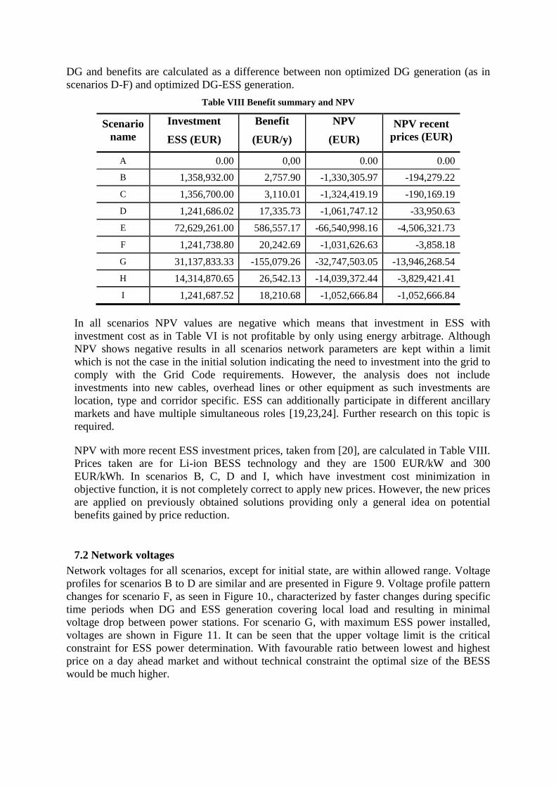
DG and benefits are calculated as a difference between non optimized DG generation (as in
scenarios D-F) and optimized DG-ESS generation.
Table VIII Benefit summary and NPV
Scenario
name
Investment
ESS (EUR)
Benefit
(EUR/y)
NPV
(EUR)
NPV recent
prices (EUR)
A 0.00 0,00 0.00 0.00
B 1,358,932.00 2,757.90 -1,330,305.97 -194,279.22
C 1,356,700.00 3,110.01 -1,324,419.19 -190,169.19
D 1,241,686.02 17,335.73 -1,061,747.12 -33,950.63
E 72,629,261.00 586,557.17 -66,540,998.16 -4,506,321.73
F 1,241,738.80 20,242.69 -1,031,626.63 -3,858.18
G 31,137,833.33 -155,079.26 -32,747,503.05 -13,946,268.54
H 14,314,870.65 26,542.13 -14,039,372.44 -3,829,421.41
I 1,241,687.52 18,210.68 -1,052,666.84 -1,052,666.84
In all scenarios NPV values are negative which means that investment in ESS with
investment cost as in Table VI is not profitable by only using energy arbitrage. Although
NPV shows negative results in all scenarios network parameters are kept within a limit
which is not the case in the initial solution indicating the need to investment into the grid to
comply with the Grid Code requirements. However, the analysis does not include
investments into new cables, overhead lines or other equipment as such investments are
location, type and corridor specific. ESS can additionally participate in different ancillary
markets and have multiple simultaneous roles [19,23,24]. Further research on this topic is
required.
NPV with more recent ESS investment prices, taken from [20], are calculated in Table VIII.
Prices taken are for Li-ion BESS technology and they are 1500 EUR/kW and 300
EUR/kWh. In scenarios B, C, D and I, which have investment cost minimization in
objective function, it is not completely correct to apply new prices. However, the new prices
are applied on previously obtained solutions providing only a general idea on potential
benefits gained by price reduction.
7.2 Network voltages
Network voltages for all scenarios, except for initial state, are within allowed range. Voltage
profiles for scenarios B to D are similar and are presented in Figure 9. Voltage profile pattern
changes for scenario F, as seen in Figure 10., characterized by faster changes during specific
time periods when DG and ESS generation covering local load and resulting in minimal
voltage drop between power stations. For scenario G, with maximum ESS power installed,
voltages are shown in Figure 11. It can be seen that the upper voltage limit is the critical
constraint for ESS power determination. With favourable ratio between lowest and highest
price on a day ahead market and without technical constraint the optimal size of the BESS
would be much higher.

If requested and properly incentivized, ESS can be used to eliminate sudden voltage
deviations and sags. The model presented in Section 6 can be easily expanded to include
additional constraints.
Figure 9 Voltages – Scenario D
Figure 10 Voltages - Scenario F

Figure 11 Voltages - Scenario G
7.3 Network losses
Table IX Network losses
Scenario
name
Losses
(kwh/w)
Difference
%
A 13,503.32 0.00
B 13,368.17 1.00
C 13,271.21 1.72
D 7,964.26 41.02
E 13,853.73 -2.59
F 8,147.48 39.66
G 65,133.72 -382.35
H 8,368.23 38.03
I 8,027.19 40.55
Figure 12 shows dynamic network losses for scenarios A to D. Scenarios B and C have
similar pattern as initial scenario A. They charge ESS in periods of low demand and discharge
it in high loading periods to exploit square dependency between connection loading and
losses. In scenario D the influence of DG can be noticed during daylight time. Energy stored
in the ESS is discharged during high loading hours and during those hours power loss profile
is similar to those in previous scenarios. Total losses are on the other hand around 40% lower.

Figure 12 Network losses - scenarios A, B, C and D
In Figure 13 losses for scenarios which maximize profit and minimize losses are presented.
Losses from initial scenario A are used as a reference for comparison. While scenario E losses
are in the same range as the ones without installed DG, in scenario F it can be notice a 40%
reduction compared to scenario C. The reason for comparing those particular scenarios can be
explained with similar EES size and power, however adding distributed units in scenario F
implies a possible increase in power losses. Optimal management of DG and EES actually
negates this and helps the DSO to reduce them even further.
Figure 13 Network losses - scenarios E and F
In Figure 14 distribution network losses for scenarios G to I are presented. As the objective
function of scenario G does not have minimization of losses included they reach high values,
up to 5 MW. This is the result of injecting most of the produced power during the daily
peaking prices. Although scenarios H and I have similar network losses (around 40% less
then in the initial solution) scenario H has much larger ESS-DG installations. Similar to
scenario D they exploit DG generation during daylight hours and lower total losses by
discharging accumulated energy during high loading hours.

Figure 14 Network losses - scenarios G, H and I
8. POWER GENERATION
Figure 15 shows charging/discharging behaviour of EES for scenarios minimizing power
losses and investments; scenarios B, C and D (discharging values are positive, and charging
values are negative). In cases without DG, scenarios B and D, ESS is charged during the night
and discharged during high loading periods. In scenario D, when DG is introduced, the
algorithm minimizes losses by charging EES during high PV generation periods resulting in
time shift for charge/discharge patterns (presented as green line).
Figure 15 Total ESS generation - scenarios B, C and D
For cases E and F driven by profit maximization and minimization of network losses, ESS
stores energy during low prices and returns it into the grid during high prices. Optimal
solution obtained for in scenario E has much larger storage capacity as power and capacity of
EES in scenario F are limited by constraints inherited from scenario C.

Figure 16 Total ESS generation - scenarios E and F
In scenarios G, H and I where ESS-DG combination can only discharge power into the
network (EES can only be charged from DG, not from the grid) all values in Figure 17 are
positive. For scenario G where only maximum profit is optimized, producer stores energy the
entire day only to discharge maximum power in the periods with maximum prices; this can be
seen as distinct daily discharge spikes. As seen in previous section with network losses, this
behaviour has very negative impact on them and generally on network loading. Discharge
patterns for scenario H are similar to the previous case during maximum prices but network
losses minimization distributes this over multiple time periods avoiding spikes and by that not
increasing losses. From Figure 17 it seems like there is a MCP threshold after which ESS-DG
starts discharging power in the network, example period 77, period 175 etc. Scenario I has a
goal to minimize investment; meaning it operates the EES-DG not to create sudden spikes
which would consequently result in higher investment cost. It basically does not store too
much PV generation to minimize investment in storage capacity and it generates energy
during high PV production hours and, in addition, during high evening demand hours.
Figure 17 Total ESS-DG generation - scenarios G, H and I

9. CONCLUSION AND FUTURE WORK
The paper attempts to provide a comprehensive modelling framework for definition of role,
size and location of electricity storages in the distribution grid. It does so by taking into
account technical constraints of the technologies, characteristics and constraints of the
distribution grid, investment costs and possibilities for providing different services to multiple
stakeholders, in case for BESS and/or DG owner and to DSO. The contribution of the
proposed concept is in creating a non bias model using direct modelling method, not
predefining optimization values or suggesting a specific storage technology. To achieve this
the paper presents an adjusted SOCP network model and MINLP based UC algorithm.
Presented results confirm that current BESS technologies do not justify their investment by
utilization of energy arbitrage only. On the other hand, by analyzing optimal size, location
and operation over a set of scenarios, they demonstrate what additional benefits BESS brings
into the future low carbon distribution grids under various control concepts. As the goal of the
paper is not to create an investment framework, the results do not capture financial benefits of
avoiding investments into the distribution grid by BESS installation.
Future work will be focused on improving the model presented in this paper, particularly on
the capability of BESS to contribute to reactive power stability. In addition, different
distribution grid types have different requirements and further research is needed to asses
these requirements.
ACKNOWLEDGMENT
This work has been supported by the European Community Seventh Framework Programme
under grant No. 285939 (ACROSS).
REFERENCES
[1] Carpinelli G, Mottola F. Optimal allocation of dispersed generators, capacitors and
distributed energy storage systems in distribution networks. Mod Electr Power Syst
(MEPS), 2010 Proc Int Symp 2010:1–6.
[2] Atwa Y, El-Saadany E. Optimal allocation of ESS in distribution systems with a high
penetration of wind energy. IEEE Trans Power Syst 2010;25:1815–22.
[3] Backhaus S, Chertkov M, Dvijotham K. Operations-based planning for placement and
sizing of energy storage in a grid with a high penetration of renewables 2011;98195.
[4] Oh H. Optimal Planning to Include Storage Devices in Power Systems. IEEE Trans
Power Syst 2011;26:1118–28.
[5] Ghofrani M, Arabali A, Etezadi-Amoli M, Fadali M. A Framework for Optimal
Placement of Energy Storage Units Within a Power System With High Wind
Penetration. IEEE Trans Sustain Energy 2013;4:434–42.

[6] Sedghi M, Aliakbar-Golkar M, Haghifam M. Distribution network expansion
considering distributed generation and storage units using modified PSO algorithm. Int
J Electr L Power Energy Syst 2013;52:221–30.
[7] Zheng Y, Dong Z, Luo F, Meng K, Qiu J, Wong K. Optimal Allocation of Energy
Storage System for Risk Mitigation of DISCOs With High Renewable Penetrations.
IEEE Trans Power Syst 2014;29:212–20.
[8] Jamian JJ, Mustafa MW, Mokhlis H, Baharudin M a. Simulation study on optimal
placement and sizing of Battery Switching Station units using Artificial Bee Colony
algorithm. Int J Electr Power Energy Syst 2014;55:592–601.
[9] Akhavan-Hejazi H, Mohsenian-Rad H. Optimal operation of independent storage
systems in energy and reserve markets with high wind penetration. IEEE Trans Smart
Grid 2014;5:1088–97.
[10] Nick M, Member S, Cherkaoui R, Member S, Paolone M. Optimal Allocation of
Dispersed Energy Storage Systems in Active Distribution Networks for Energy
Balance and Grid Support. IEEE Trans Power Syst 2014;In press:1–11.
[11] Oldewurtel F, Borsche T, Bucher M, Fortenbacher P, Gonz M, Haring T, et al. A
Framework for and Assessment of Demand Response and Energy Storage in Power
Systems a. 2013 IREP Symp., Rethymnon: 2013, p. 1–24.
[12] FICO XPRESS. Http://www.fico.com/en/products/fico-Xpress-Optimization-Suite/
n.d.
[13] Jabr R. Modeling network losses using quadratic cones. IEEE Trans Power Syst
2005;20:505–6.
[14] Jabr R a. Radial Distribution Load Flow Using Conic Programming. IEEE Trans Power
Syst 2006;21:1458–9.
[15] Jabr R a. Optimal Power Flow Using an Extended Conic Quadratic Formulation. IEEE
Trans Power Syst 2008;23:1000–8.
[16] Baran ME, Wu FF. Network Reconfiguration in Distribution Systems for Loss
Reduction and Load Balancing. IEEE Power Eng Rev 1989;9:101–2.
[17] Baran M, Wu F. Optimal capacitor placement on radial distribution systems. IEEE
Trans Power Deliv 1989;4.
[18] Farivar M, Clarke C. Inverter VAR control for distribution systems with renewables.
IEEE SmartGridComm, IEEE; 2011, p. 457–62.
[19] The Energy Research Partnership. The future role for energy storage in the UK Main
Report. Grad: 2011.
[20] Akhil AA, Huff G, Currier AB, Kaun BC, Rastler DM, Chen SB, et al. DOE / EPRI
2013 Electricity Storage Handbook in Collaboration with NRECA. Albuquerque: 2013.

[21] ELEXON Portal. Https://www.elexonportal.co.uk/
[22] SohnAssociates. OFGEM Electricity Distribution Systems Losses Non-Technical
Overview. 2009.
[23] U.S. Department of Energy. Grid Energy Storage. 2013.
[24] European Commission - Directorate-general for Energy. The future role and challanges
of Energy Storage. 2013.