Pergamon Computers Math. Applic. Vol. 33, No. 3, pp. 45-63, 1997

Copyright©1997 Elsevier Science Ltd Printed in Great Britain. All rights reserved

0898-1221/97 $17.00 + 0.00 PII: S0898-1221 (96)00236-2

Convergence Theorems for the Kohonen Feature Mapping Algori thms with V L R P s

J. F. FENG Labora tory of Biomathemat ics , The Bab raham Ins t i tu te

Cambridge CB2 4AT, Uni ted Kingdom

B. TIROZZI Mathemat ica l Depar tment , Universi ty of Rome "La Sapienza"

P.le A. Moro, 00185 Rome, I ta ly

(Received July 1996; accepted August 1996)

A b s t r a c t - - T h e convergence of the Kohonen feature mapping algorithm with vanishing learning rate parameters (VLRPs) is considered, which includes the simple competitive learning algorithm as a special case. A few examples show that the learning fails to converge to "global minima," in general. Then, we present a novel approach which enables us to find out a new family of VLRPs such that the corresponding learning algorithm converges to the set of "global minima" with probability one. The new VLRPs is a generalization of the well-known rate parameters used in the simulated annealing. A numerical example is also included to confirm our theoretical approach. We believe that this discovery is of importance for a large class of learning algorithms in neural networks and statistics.

K e y w o r d s - - K o h o n e n feature mapping algorithm, Supermartingale, Global minima, Stochastic differential equation, Vanishing learning rate parameters (VLRPs).

1. I N T R O D U C T I O N

In recent years, there are extensive research works devoted to the study of the Kohonen fea- ture mapping algorithm, both theoretically and numerically [1-3]. In [4,5], and references given therein, the authors consider the equilibrium states of the Kohonen feature mapping algorithm with the learning rate parameter independent of time. In [4], a thorough investigation of the existence and the number of the metastable states is carried out. In [6-8], the asymptotic prop- erty of the one-dimensional Kohonen feature mapping algorithm is studied. Recently, a novel approach [9] to the problem of constructing topology preserving maps is introduced, which is based upon a Hebbian adaption rule with winner-take-all like competition. Here, we first con- sider the convergence problem of the Kohonen feature mapping algorithm (see [3, p. 232]) with the nonincreasing vanishing learning rate parameters (VLRPs) ~(t) > 0, satisfying the usual restrictions found in stochastic approximation theory [10-15]

fo ° ~(u) = oo, (I) du

f0 ° ~2(u) du < (II) oo.

Partially supported by the CNR of Italy, J. F. was also partially supported by the A. von Humboldt Foundation of Germany.

Typeset by AA/cS-TEX

45

46 J . F . FENG AND B. TIROZZI

The constraints (I) and (II) above are usually imposed for the stochastic approximation algorithm (see, for example [10,12-14]), and the reason for a family of learning rate parameters satisfying them is fully explained in [10,14]. See also, Section 3 of the present paper, where we assert that the condition (II) is not a necessary one. Examples in Section 3 show that, in general, there are metastable states for the algorithm. Note that a Canonical candidate of ~(t) under the restrictions (I) and (II) will be

1 ~(t) = t-- ~,

for 1/2 < a _< 1 (see [3, p. 223; 15, p. 259]). The above conclusions naturally suggest to us to ask the question: does it exist a general rule

(VLRPs) for the learning algorithm which allows the system to get out of the metastable states? In other words, we look for a family of VLRPs which has a role like the decreasing ' temperature' in simulated annealing. Nevertheless, an example in Section 3 of the present paper indicates that under the constraints (I) and (II), the learning algorithm will stay at some local minima with a positive probability.

It was first noted in [15, p. 259] that in a linear learning algorithm with VLRPs the restric- tion (II) above is unnecessary and it could be replaced by a much weaker condition

lim r/(t) = O. (II') t---*O0

Based upon the self-similarity property of Brownian motion and results of simulated annealing in [16], we present a novel and rigorous approach to determine a new family of VLRPs. This new family of VLRPs which is between 1/log t and 1 / ~ , ensures that the learning algorithm with the VLRPs escapes from the local minima and reaches the desired global minima with probability one. This fact is shown in Section 3. Note that this family of VLRPs fulfills the restriction (I) and violates the restriction (II), but it satisfies (I) and (II'). We believe that our discovery is of general guidance for a class of learning algorithms with VLRPs, such as the learning algorithm of Oja's law [3], Hebb learning [17], the em and EM algorithms [18], and some most recently proposed algorithms like [19,20], etc.

2. A C O N V E R G E N C E T H E O R E M

2 . 1 . N o t a t i o n a n d R e s u l t s

For a concrete description of our result, we first briefly review the Kohonen feature mapping algorithm in detail.

In the Kohonen feature mapping algorithm, there is a single layer of output units Oi(n) E {1, 0}, i = 1 , . . . , N at time n, each fully connected to a set of inputs ~j(n), j = 1 , . . . , M, via connections w~j(n). In the sequel, we assume that the inputs ~j(n), j = 1 , . . . , M are chosen independently according to a probability distribution P. For each presentation of the input ~j(n), j = 1 , . . . , M we choose one of the output units, called the winner. The winner is the output unit with the smallest distance between its connections and the inputs

I1~,(=) - ~(=)11,

for vectors w~(n) = (w~j(n),j = 1 , . . . , M), ~(n) = (~j(n),j = 1 , . . . , M), where ]]. II represents the Euclidean norm. Let I(., .) be the function:

_r(wi(n), ~(n + 1)) = I{llw,(,~)-~(n+l)ll<Jl~j(n)-~(=+l)llJ#i} (wi(n), ~(n + 1)),

where IA is the indicator function, i.e., IA(X) = 1 if X E A and IA(X) = 0 if x ~ A.

Convergence Theorems 47

The Kohonen feature mapping algorithm ensures the weights update decreasingly according to

its distance with respect to the winner

wij (n Jr I) ---- wij (n) -b ~(n) ~ A(i, k ) i (wk(n), ~(n Jr 1)). (~j (n -b i) - w ~ j (n)) , k

(i)

i -- 1 , . . . , N , j -- 1 , . . . , M or in vector form

wi(n q- 1) = wi(n) Jr 77(n) ~ A(i, k) f (wk(n), ~(n + 1)). (~(n q- 1) - wi(n)), k

(2)

where ~(n) is the positive learning parameter ~/(0) < 1, ~?(n) > r/(n q- 1), and A(i , j ) is a nonin- creasing function of H i - j II. If A(i, j ) = ~iij, the above algorithm is called the simple competitive learning.

After the learning procedure is finished, any set of input vectors will be partitioned into nonover- lapping clusters. This means that a new incoming signal ~(n ÷ 1) is classified as the pat tern i if it is closest to the weight wi. In other words, the new signal ~(n + 1) is recognized to be of the

type wi, if and only if

IIw - ÷ 1)11 _< I1 ¢ + 1)tl, j # i .

Note that the nonlinearity of the dynamics above is addressed by the function I. In the case considered in [15, p. 279], N = 1, and so the dynamics defined by (1) is linear because there is no competition at all. Furthermore, when A(i,i) -- 1 and A( i , j ) = 0 for i ¢ j , this case is exactly the simple competitive learning algorithm.

For a compact region 12 of R M, let us introduce the definition of Voronoi tessellation associated

with a family of vectors y = (Yi, i = 1 , . . . N) E ~.

DEFINITION 1. For a given compact subset 12 E R M, the Voronoi tessellation II(y) = (II(y)i, i -- 1 , . . . , N) associated with a family of vectors y l , . . . ,YN is a partition off~ given by

1-I(y)~ = {x,[[yi- x[[ <_ ][yj - x[[,j ¢ i}, i = l , . . . , N .

Let us define a function g which is the leading term of the supermartingale difference given in the proof of Theorem 2.

g (Yl, Y2,. . . , YN; Wl, w2, . . . , WN) = ~ (y~ -- Wi)" h(k, i)(z - y~)f(x) dx . i----1 (Y)k

g depends on the vectors w = (Wl,W2,... ,WN), y = (Yl,Y2,... ,YN) E ~ M x N . f is the density of the distribution P with support on a compact region ~ of RM, H(y) = (Yi(y)i, i = 1 , . . . , N) is the Voronoi tessellation associated with y = (y , , . . . , YN).

We define also:

O := {the set of all Voronoi tessellations associated with { w l ( n ) , . . . , wN(n)}, for all n}.

For Yl , . . - , YN E R M, we use the convention that y = ( y l , . . - , YN) E O implies tha t there exists a Voronoi tessellation II(y) such that {II(y)i, i = 1 , . . . N} E O.

Now we state the main theorem of this section.

THEOREM 2. /~ there exists a unique point (ZOl, w2 , . . . , WN) e R MxN, such that

g(Yl , . . . ,YN; Wl, . . . ,WN) ~_ O, Vy E e , (3)

48 J.F. FENG AND B. TIROZZI

where the equality holds, i f and only i f yi = wi, i = 1, . . . ,N , and

E ~(n) =oo, 7'1,

n

then we almost surely have

(4)

for

such that

Z l <: Z2 < " ' " < Z N ,

N

(w(n)) = E E / n A(k,i)IIx - w i (n) l l2 f (x )dx gl i = 1 k ( w ( n ) ~ )

and w(n) = (wl(n), w2(n) , . . . , w(n)). Since 91(w(n)) is uniformly bounded by a constant A the inequality (5) thus, becomes

N

E [ E ([[wi(n + 1) -wi[[ 2 [ I n ) - Hwi(n) -wi[[ 2] i = 1

< ~(~)g (~(~), ~) + v(n)~A (6)

<_ ~(n)g (w(n),w) + ~(n)2A 1 + ~ IIw~(n) - w~ll ~ • i = l

In terms of [14, Theorem 7.1, p. 43] together with Theorem 5 of the present paper, we arrive at the desired conclusions. |

Let us say a few words concerning condition (2). The fulfillment of condition (2) ensures that the learning algorithm moves downhill in the energy landscape, and so the uniqueness of the limit of the learning algorithm is true under condition (2). In Section 3, we will give a new family of learning rate parameters when condition (2) is violated, which is certainly the more interesting c a s e .

For a one-dimensional input signal, i.e., M = 1, without loss of generality, we can assume that a < Wl(0) < w2(0) < ..- < wg(O) <_ b with fl = [a,b]. In this setting, we are able to simplify condition (2) in Theorem 2 due to the fact that the simple competitive learning does not change the order of weights a < wl (n) < w2(n) < . . . < w g ( n ) <_ b, n > 1.

LEMMA 3. H M = 1, then Yl . . . . ,YN e (9 / / 'and only ira < Yl < "'" < YN ~ b.

PROOF. "==~." First note that if wl(0) < w2(0) < . . . < wg(O), in the simple competitive learning, we still have wl(n) < w2(n) < . . . < WN(n), for n > 0. Suppose that there is a Voronoi tessellation I I e (9, then there exist

i = 1 , . . . , N ,

here (z0 + z l ) /2 = a and (ZN+l + z g ) / 2 = b. So y 6 e implies that a < Yl < Y2 < "'" < YN <-- b. " ~ . " Trivial. |

By combining Lemma 3 and Theorem 2, we have the following corollary. Three examples which explain the application of the next corollary are presented in Section 2.2.

lim w~(n) = w~, i = 1 , . . . , N . ~ ---}CX)

PROOF. We need to introduce some more notation. Let .7" n be the sigma algebra generated by ~(k), k <_ n, E(~ I ~-~) is the conditional expectation for the random variable ~ with respect to the sigma algebra ~-n. In terms of the proof of Theorem 5, below we see that

N

y ~ [E (llw~(n + 1) - w~ll 2 I Y . ) - IIw~(n) - w, II ~] < ,l(n)g (w(n), w) + r/(n)2gl (w(n)), (5)

Convergence Theorems 49

COROLLARY 4. I f there exists a unique point ( w l , . . . , WN) C R N, such that the inequality

w l , . w N ) (yl - . . , = h(k, 1) (x - Yl) f ( z ) dx k J ( ( Y k - l - k y k ) / 2

N - 1 /" (Yk+ 1Tyk ) / 2

+ ~ (Yi - wi) ~ / c A(k, i) (x - yi) f ( z ) dx i=2 k (~k_l+y~)/2

)_:~ /(yk+~+yk)/2 A(k, N) (x - YN) f ( x ) dx -k (YN -- WN) k J(y~_l+yk)/2

< 0 ,

holds for a <_ Yl < "'" < YN <-- b, except for yi = wi, i = 1 , . . . ,N , and

~(n) = co, ~ ~72(n) < co, n n

then we almost surely have

lim w/(n) = wi, i = 1 , . . . , N . n -'-* O0

In the next theorem, we consider the convergence rate of the simple competitive learning. We prove that, under the conditions in Theorem 2, the algorithm will achieve the given accuracy within a finite number of updates.

We define T(e) = inf{n, llwi(n) -- will <_ e, i = 1 , . . . , g }

as the first time that the training error is less than e.

THEOREM 5. In the circumstances of Theorem 2, there exists a constant

> o,

such that we have almost surely T(e) < B(e).

PROOF. We find a negative bound for the difference:

N

[Z (Hwi(n + 1) - will 2 I I n ) - Ilwi(n) - will2], i=1

and from it we get that E(llw/(n + 1) - w/ll 2) is a supermartingale. According to the definition of the algorithm, we have

÷ Will 2 E

= E (llwi(n + 1)1] 2 I 9rn) - 2wi. E (wi(n + 1) I I n ) + Ilwill 2 - IIw/(n) - w / l l 2

= 2r/(n) (wi(n) - wi ) . E ((~(n + 1) - wi(n)) I (wi(n), ~(n + 1)) ] ~'n)

+ 772(n)E ([l~(n + 1) - w/(n)[[ 2 1 (w/(n),~(n + 1)) [ ~-n).

Since wi(n) and ~(n + 1) are in the set

{ll~(n + 1) - wi(n)l I < II~(n + 1) - wj(n)lI, j # i } ,

50 J . F . FENG AND B. TIROZZI

if and only if

~(n + 1) 6 n(w(n))~,

for w(n) = (w~(n), i = 1, . . . , N), wi(n) and ~(n + 1) are independent, we yield that

~(n) (wi(n) - w,) . E ((~(n + 1) - wi(n))I (wi(n),~(n + 1)) I $'~)

= ~(n) (wi(n) - wi). E [ h(k, i) (x - wi(n)) f (x) dx k dII(w(n))k

(7)

and

~(n)2E (ll~(n + 1) - ~,(~)112 ~ (~,(~), ~(~ + 1)) l y e )

: ~?2(n) E f k JII(w(n))k

A(k,i) IIx - wi(n)H 2 f (x)dx . (8)

Furthermore, if we replace the time n in equality (7) and (8) by the stopping time an := T(e) A n = min(n, T(e)) all equalities hold. From the definition of the stopping time and condition (2) in Theorem 2, we see that

g ( W l ( O ' n ) , . . . , W N ( a n ) ; Wl , . . . ,WN) N P

= Z (W(an)i - wi)" Z / h(k, i) (x - w(O'n)i ) f (x) dx i=l k dn(w(a~))k

<_ -h(e) < 0,

(9)

for a number h(e) depending only on e. By condition (3) of Theorem 2, for n large enough, the sign of the term

N

?~(n) Ei=I (W(an)i-- Wi) '~k- fri(w(~.))k A(k, i ) ( x - w ( a n ) i ) f ( x ) d x

N + r/2(n) E E / n h(k, i)]Ix - - w(crnliH 2 f (x) dx

i=l k (wC~))k

is determined by the sign of the following term

g (wl(an), . . . ,WN(O,); Wl, . . . ,WN) N P

= ~ (~(~,-), - ~ ) ~ l A(k, ~) (~ - ~(a ,O,) / (~) az i = l k dH(w(a,))k

and so is negative, and we denote it -h i ( e ) < 0. This explains the reason why we introduce the function g in Section 2. Without loss of generality, we assume that (9) is true for n > 1. We consider again the term

N an -- i

II~,(a~) - ~,112 + ~ hl(~l~(k). i=1 k=l

After repeating the same argument as before, we conclude that it is still a nonnegative super- martingale and so is

N a,~-I IIw,(a.) - w, II 2 + ~ hl(~ln(k).

i= i k---I

C o n v e r g e n c e T h e o r e m s 51

and

By the convergence of the supermartingale, the limit of

are both finite almost surely. Thus,

N a~-I

t1~(o . ) - ~11 ~ + ~ h~(~l~(k) i=1 k = l

N

i=1

lim an = lim T(e) A n < B, n'-~OO ?l--* OO

almost surely for an integer B satisfying

B N

~_~l(k)hl(e) > N max Hx - yll 2 > ~ Ilwi(n) - w~ll 2, x,yEl~

k-~l i=1

which implies

k/n,

~(~) < B

almost surely. Note that the random time T(e) is bounded by a deterministic quantity B. |

Although that wi(n), i = 1 , . . . , N is a stochastic process, Theorem 5 asserts tha t within a finite and a deterministic time B(e) wi(n), i = 1 , . . . , N will reach a given accuracy e.

2.2. E x a m p l e s

In this section, in order to show the applications of the theorems of the previous section, we consider three typical examples, in the sense that the first example takes into account the case when the input data set is discrete, the second and the third example consider the case when the input data set is continuously distributed according to the uniform distribution and the normal distribution, respectively. We consider only the case of simple competitive learning.

EXAMPLE i. Suppose that f ( x ) = ~-~N=I cdfw, (x), w i t h ~-'~N=I C i = 1 for wi E [a, b] C R 1, c~ > 0, i = 1 , . . . , N , and wl < w2 < . . . < WN. Then we have that

g ( Y l , . • • , YN; Wl,. . . , WN) = --Cl (Yl -- W l ) 2 I[,~,(v1+~2)/21 ( W l )

N - 1

-- ~ Ci (Yi -- Wi) 2 I[(y ,_,+y,) /2 ,(y ,+y,+l) /2 ] (Wi) i-~2

-- CN ( Y N -- W N ) 2 I [ (yN+YN+I) /2 ,b](WN).

From the theorems of the previous section, we can conclude that

= ( ~ I , . . . , ~ N )

is the unique attracting point of the dynamics (1). The proof of Theorem 2 shows that the function g is the main contribution to the derivative of a Liapunov function. In fact, the quantity

N

[E ( i lw,(n + 1) - w, l121 ~=n)] i = l

introduced in the proof can be considered to be the Liapunov function of the system. The difference appearing in the submartingale condition:

N

÷ i ,ll i----1

52 J F FENO AND B TIROZZI

can be considered as a discretized derivative and is the sum of two terms. The one different from g vanishes. The points ( Y z , . . . , YN) which make the function g equal to zero can be interpreted as the minima of this Liapunov function. Using this terminology one may say that the dynamics (1) will converge to the global minima Yl = w l , . . . , YN -~ w g if the hypothesis of the Theorem 2 is satisfied. If there are many points for which the equality g =- 0 is verified, then they may be seen as local minima which can trap the dynamics. The condition ensuring that there is a unique solution (Yl , . . . , YN) of the equation

g ( Y z , . . . , yN; w l , . . . , WN) : 0

is quite restrictive. In general, there are (infinitely) many solutions of it. Hence, the development

of an algorithm to avoid the metastable states is of general importance, which is the content of the next section.

EXAMPLE 2. Suppose that ~(n) is uniformly distributed over the interval [0, 1]. We are going to

prove that wl = 1/4, w~ = 3/4, and g(y, w) is negative except for Yl = wz and Y2 -- w2. First note, that in this situation we have

f ( Y z + y2)/2 / 1 g(y, w) = (Yz -- w l ) (x - Yl)dx + (Y2 - w2) (x - Y2)dz.

JO (~,+v2)/2

Therefore,

g(y, w) = (Yl - Wl) ~- I x - Yl) dx + (Y2 - w2) + (x - Y2) dz J y l / 1 - } - y 2 ) / 2 2

( 2 X(yl y2) 2 ) ( X ( y z - - y 2 ) 2 + l ( 1 _ y 2 ) 2 ) ---- ( Y l - - W l ) - - y 2 + 2 4 -{- ( Y 2 - - W 2 ) 2 4 2 '

It is easy to check numerically (Figure 1) that Wl = 1/4, w2 = 3/4 is the unique point for g(y, w) = O. Therefore, from Corollary 4 and Theorem 5 of the previous section, we have

1 3 lim w2(n) lim wz(n) = "~, n~oo = 4 '

n ---~OO

and ~'~ > 0, 3B(~) > 0, <

(Yl "0"25)*('O'5"yl'y 1 +0"1-~'5-:1Y 1"y2)"2)+ly2"0"75)'(IO" 125" (Y 1"y2)"2+O-S'(1-y2)"20 )

........... . . . . : . : ...... :!i ::!i: . . . . . . . . . : . : : ........

0 "" " : " . . . . . "*" . . . . . ~'": " : " . . . . . . "°" " ' : ~ : " : "'" " . . . . . ~"" "; . . . . . . . o " : ,~ . . . . oo . . . . . ~ : .~ ' - - . . .w . . " --~.,... .* - . . . . o ~- . . .o .- .*~ . . . . . .- - - . . . °- . - - . . . ¢ ,oo" "-*~:.o oO - - . . . . . . ":,.. . . . . . . . . - . . . . . , , : : . : . . . . . . .*- - - : , .

- 0 . 1 - " . . . . . - " : ' " . . . . . - . . . . . ~ : . . - ~ . . . . . . . " • . o o . . o * - r , . . . oo " - . - ~ : o - - . . . . o - " - . . . ~ : o . oO • . . . . . . o

-0.2. " " "--"" " ' : ' : . . . . " -0.3

-0.4

-0.5

-0.6

1

0 0.5

! 0

Figure 1. The function g defined in Example 2 of Section 2.

C o n v e r g e n c e T h e o r e m s 53

EXAMPLE 3. Suppose tha t ~(n) is distributed with density function

l e x p ( X ' ~ ) I [ - K , K ] ( X ) , f ( z ) = c

the restriction of the normal distribution with mean 0 and variance 1 to I - K , K], where K = 2

and c = f_K Ke -(x:/2)dx. I t is natural to expect that wi = - 1 / 2 c ( 1 - e -K~/2) = 0.18 and

w~ = 1/2c(1 - e-K~/~).

Let

g ( y ~ W) (Yl ? / 2 1 ) f ( y 1 - F y 2 ) / 2 - ( z - Y l ) e - x ' / 2 d x + (Y2 - w 2 ) fK _ - - (X y2)e -x~/2 dx J - K J(yiTy~)/2

_ _ f ( , ~ + ~ ) / 2 ---- - - ( Y l - - W l ) 1 e -(y~+y~)~/s (Yl w l ) Y l J - K e -x2 /2 dx

1 + ~ e -K:/2 (y~ - y: - Wl + W2) -~- (Y2 - - W 2 ) ~ e -(yl+y~)2/8

/: - (y~ - w ~ ) y ~ e - ~ / ~ d x . l + y ~ ) / 2

I t is easy to check numerically (see Figure 2) that the condition of Corollary 4 on the function g

is not true, i.e., there are several points (yl, y~), y~ < Y2 such that g(yz, Y2; Wl, w~) -- 0.

o..-. ' . . . o O ~ - - ° ° ° ° ~ . . .~:: . . . . . . : ...... :~:::. ::: ....... ~.

., . . . . . . ,-~." F¢',~...~ .~.-~ • ~,.,~-.~-:" ~:.. . . . . . . .,°- . . . . . :,,: . . . . ..~ . . . . . . o -° ° - - . ° ~ . * ~ . . • - ~ o ° * - . ° --w. ... . . . . . . . . ~:: ya : . . . . . , j . . -~-~¢1... .,. . . . . . . ~::- -::~: . . . . . ,,.. . . . . . :~.-

° . o o ° . ° ° o° . . . . . .~ :o° o . ~ ' - ° . ~ p ° o " ~ . . . . . . . o . . . . . . . : . o° " ° - ° ° ° r ° o ...:: . . . . .: . . . . . . . ~::" "'_;,: . . . . . . . " . . . . . :~::. . ..: . . . . . . . ~::" " ' : : , : . . . . . ..

U [ ~ ' - . . . . . - " " " r - * * . . ." "°- , - .* :° . : ' *°°- . .°s. . .° "°:.*: . . . . °" ] ~ " . . . . ~ :'~c~., . :-" ":'," . . . . . . . • . . . . . :,,: . . . . .. " . . . . . ,.:: ::," . . . . . . •

0.5 0 . 5

-2 -1.5 -1 0 5 " " 0 -1

F i g u r e 2. T h e f u n c t i o n g de f ined in E x a m p l e 3 of Sec t ion 2. N o t e t h a t t h e r e a re seve ra l p o i n t s (yz, y2) w i t h t h e p r o p e r t y g(yz, y2; wz, w2) = O.

3. A N E W F A M I L Y OF V L R P S

In Section 2, we developed a condition for the convergence of simple competit ive learning with VLRPs. However, it is readily seen from our examples that , except for some special case (Example 2), the convergence of the algorithm will fail in general. On the other hand, all the algorithms similar to the simple competit ive learning with VLRPs are in danger of getting caught in some local useless minima [4]. Hence, the problem of getting out of local minima is of general importance for the learning algorithms with VLRPs.

Essentially, a learning algorithm as we considered in Section 2 with VLRPs, can be written as

dXt = ~(t) (b(Xt) dt + ~(t) dBt) , (10)

54 J.F. FENO AND B. TIROZZI

for xt C ]~M×N, b(.) a measurable function on R M×N, t E R +, and ~/(t), the VLRPs with 7(0) _> 0, ~(t) < rl(s) if t _> s, f~(t) > 0. Note that the discretized equation corresponding to (10) is

Xn+l = Xn + hrl(n)b(X,~) + ~(n)vfhWn, (11)

where h is the step-size, W~ is normally distributed with zero mean, and covariance equal to the unit matrix I. For the purpose of finding a family of appropriate VLRPs in self-organizing Kohonen algorithm, equation (10) has been discussed in [15] from the Fokker-Planck equation point of view. In fact, in the field of neural networks, there are many learning algorithms developed with VLRPs and they are special cases of (10), for example, the network with Oja's rule [3], self-organizing Kohonen algorithm, the algorithm proposed in [18, p. 64], the dynamic link network [21,22], etc.

In this section, we first consider how to choose r/(t) and fl(t) so that Xt converges to the global minima of U if b = -g rad U. It is proved in Theorem 6 below, that under the usual restriction (I) of Section 1 on ~(t),/3(t) should take the form (see Theorem 6)

~

~/~/(t) log fo ~(u) du

Note, that as ~;(t) = c a constant independent of time, Theorem 6 reduces to the well-known results of simulated annealing [16].

Second, if the signal is not separable from the noise, this means that in the equation (10) we require f~(t) -- 1,Vt. It is shown in Theorem 7 below, that if the family of VLRPs ~;(t) satisfies an ODE, the solution of which is between 1/log t and 1 / v / I ~ , then Xt will converge to the global minima with probability one. It is worthwhile to point out that this family of VLRPs already does not satisfy the restriction (II) of Section 1. We believe that the discovery of this section is of general importance, also for some well-known statistical algorithms such as Robbis- Monro procedure and Kiefer-Wolfowitz procedure, which have been intensively studied in the statistics (see [10,11,13,14]) and take the form of (10). For the neural network applications of these algorithms we refer the reader to [23, Chapter 2].

3.1. T h e G e n e r a l Case

In this section, we consider equation (10):

dXt = ~?(t) (b(Xt) dt + ~(t) dBt) .

In order to develop a new learning rate for ensuring the convergence of the algorithm to the global minima, we apply the results of simulated annealing to our case [16]. However, simu- lated annealing corresponds to the case in which the dynamics without noise is homogeneous, namely ~(t) is a constant independent of time t, and the noise goes to zero as the system evolves. This requires that in (10), the coefficient in front of b should be independent of t, while there is still a vanishing rate before the Brownian motion Bt. Fortunately, after taking another time scaling, we are able to remove the vanishing term in front of the drift term b, and keep the second term of the noise as a standard Brownian motion because of the self-similarity property of the Brownian motion. Furthermore, there is still a vanishing rate multiplying the Brownian motion.

Before going to more general cases, we show here first an example, in order to explain our general ideas above.

EXAMPLE 4. Take ~(t) = 1/t, ~(t) = 1, M = N = 1 in equation (10). Note that in this setting, the conditions (I) and (II) of Section 1 are fulfilled for the choice of r/(t). Now the dynamics (10) reads

1 dZt = ~ (b(Zt) dt + dBt) .

Convergence Theorems 55

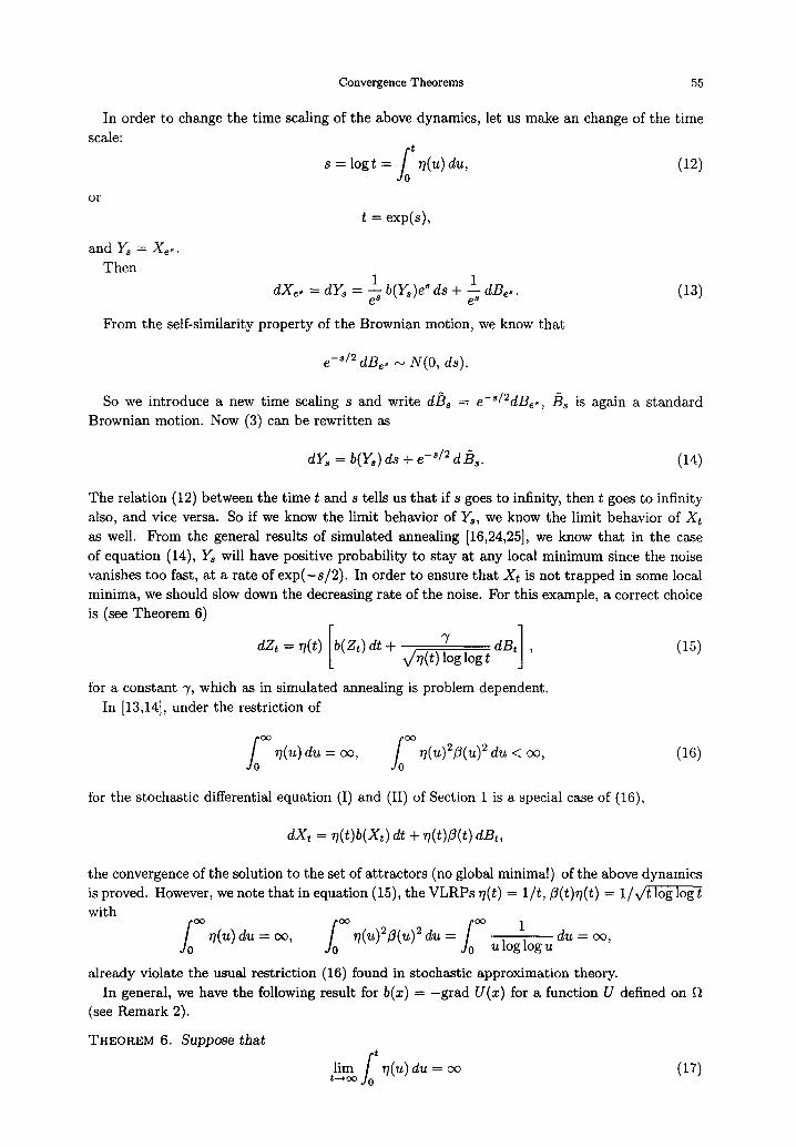
In order to change the time scaling of the above dynamics, let us make an change of the time scale:

f s = log t = ~(u) du, (12)

or

t = exp(s),

and gs = Xe.. Then

dXe. = dY~ = __1 b(Y~)e ~ ds + _1 dBe.. e s e s

From the self-similarity property of the Brownian motion, we know that

(13)

e - s / 2 dBes .- N(O, ds).

So we introduce a new time scaling s and write d/38 = e-8/2dBe~, [3s is again a standard Brownian motion. Now (3) can be rewritten as

dYs = b(Ys) ds + e -s/2 dBs. (14)

The relation (12) between the time t and s tells us that if s goes to infinity, then t goes to infinity also, and vice versa. So if we know the limit behavior of Ys, we know the limit behavior of Xt as well. From the general results of simulated annealing [16,24,25], we know that in the case of equation (14), Ys will have positive probability to stay at any local minimum since the noise vanishes too fast, at a rate of exp ( - s / 2 ) . In order to ensure that Xt is not t rapped in some local minima, we should slow down the decreasing rate of the noise. For this example, a correct choice is (see Theorem 6)

[ ~ dBt I , (15) dZt = ~?(t) b(Zt)dt + X/fl(t) loglogt

for a constant 7, which as in simulated annealing is problem dependent. In [13,14], under the restriction of

f0 V(u) du = c~, ~?(u)2/3(u) 2 du < c~, (16)

for the stochastic differential equation (I) and (II) of Section 1 is a special case of (16),

dXt = ~(t)b(Xt) dt + ~(t)fl(t) dBt,

the convergence of the solution to the set of attractors (no global minima!) of the above dynamics is proved. However, we note that in equation (15), the VLRPs ~?(t) = l / t , j3(t)~?(t) = 1]~/t log log t with

•(u) du = c~, ~?(u)213(u) 2 du : u log log u du = c~,

already violate the usual restriction (16) found in stochastic approximation theory.

In general, we have the following result for b(x) = - g r a d U(x) for a function U defined on fl (see Remark 2).

THEOREM 6. Suppose that

-Jot = (l W)

56 J.F. FENG AND B. TIROZZl

and F ,1

dZt = 77(t) [b(Zt) dt + 3" dBt[ (18) [ log J where Zt E ~t, a compact subset o f R M×N, b is a measurable function on C1(~), and Bt is the

M × N-dimensional Brownian motion. Then there exists a constant 3'0, and a set A C ~ such

that as 3" > 3"0, we have lira P ( Z t E A ) = I ,

t---*O0

where A is the set of global min ima of U.

PROOF. Let

i' s -- s ( t ) = , ( u ) e ~ (19)

denote its inverse function as t = t(s). Define

Y~ = Zt = Zt(~).

Then the equation (18) becomes

dYs = b(Ys) ds + 3"v/-~--~ dBt. (20)

In terms of the self-similarity property of the Brownian motion and rl(t)dt = ds, we derive that

d/~s := ~ dBt(s) ~ N(0, ds . I ) ,

where I is the (M x N) x (M x N) unit matrix. H e n c e , / ~ is still a standard Brownian motion on ~M×N. Now (18) becomes

~/ d/~s. dYs = b(Ys) ds + (21)

From the condition of the present theorem, we see that

s(t) --, oo, as t -~ oo,

and

Therefore, we have

t (s ) ~ o o , ~ s ~ .

lim P ( Z t e F ) = lim P( ]IseF) , t ----~OO 8----*00

for any measurable subset F of R M. By theorems of [16], we deduce that there is a positive constant 3'o such that as 3' > 3'o,

lim P ( Z t E A) = lim P(Ys E A), t---~OO 8---~OO

where A is the set of the minima of U as b(x) = - g r a d U(x).

REMARK 1. In Theorem 6, 3"0 could be (roughly) chosen to equal to

~ 2 ( s u p U ( x ) - inf U(x)~. \xEfl zE~2 ,/

Convergence Theorems 57

REMARK 2. If there is no energy function U for the dynamics, the action functional defined by

{ 1/0 A(x,y) = i~f S0,T(¢);S0,T(¢) = ~ I1¢~ -b (¢ t )H 2 dt,

¢ E C[0,T ] (RM), ¢0 ---~ z, Cr ---~ Y, VT ~ 0 ~ , J

could be used to replace U and

V0- -4 /2 sup A(x,y) . V x,yE~

Similar results as in the above theorem are still true, see [16,24].

REMARK 3. Our approach also yields a conclusion which is already noted in [15, p. 259]. When b(x) = - x in equation (10), it is pointed out in [15, p. 259], that the second condition (II) of

Section 1, i.e.,

f0 °° r/2(u) du < OO

can be replaced by a much weaker condition

lim r/(t) = 0, $ ---*CX)

and the conditions

fo °° rl(u)du --- c~, lim ~(t) = 0, ~----*OO

are necessary and sufficient for Xt to converge to O. In fact, our approach also rigorously yields this result. Consider the equation of Xt

dXt = ~?(t) [b(Xt) dt + dBt] .

After taking the new time scaling s (see the proof of Theorem 6), we yield that

dye = b(Ys)ds + v/~-(s) d/)s,

if ~(t) = ~?(t(s)) --* 0 and U(z) only one minimum, say x0 (the case considered in [15] x0 = 0), we know that Xt --* z0, a.s. This proves the sufficiency. The necessary condition is obvious since if ~(t) does not go to zero, Ys will certainly not stay at x0 at all.

REMARK 4. We can of course choose a family of VRLPs decreasing more slowly, and at the same time ensure that the conclusions of Theorem 6 axe still true. For example, if we set

~(t) = I r / ( t ) log log fo ~(u)du'

then we still have the conclusions of Theorem 6.

3.2. A Special Case

In some situations, it is not possible to separate the drift term b from the Brownian motion Bt. And sometimes the data sent as an input to the network is noise-contaminated also. This is equivalent to asking if there exists a family of r/(t) such that Xt converges to the global minima of U, where Xt is the solution of

dXt = ~(t) (b(Xt) dt + dBt) .

58 J.F. FENG AND B. TIRozzI

From Theorem 6, we know that above requirement is equivalent to say that for t _> 1

~(t) log v(u) du = .y2

or

fot @ log V(u) du = ,(t---~"

Differentiating on both sides of the equation above, we have

~(t) ~'(t)~ ~

f ~ ( ~ ) d ~ = ~(t)~

or

(22)

r/3(t) ~ ' ( t ) = 2 ~ (23)

If we are able to solve the above equation and prove that its solution satisfies the conditions of Theorem 6, we obtain a family of new VLRPs r/(t), r/(t) could be easily computed numerically (Figure 3) and we have the following estimate.

0.9

0.8

0,7

0.6

0.5

0.4

0.3

| ' I | I | . . . . . . . | . . . . . . . i I !

eta(t) 1,4o9(,,+I)

%%.

h "°%"° '° ' °°"° . . . . . . . . . . . . . . . . . . . . . . . . . " . . . . . . . . . . . . . . . .

0.2

0 .4J I .. ( ! ! I t I _ . ! !

0 100 200 300 400 500 600 700 800 900 1000

Figure 3. Tile function ~?(t) with 0' = 1 defined in Theorem 7. of Section 3.

In terms of the nonincreasing property of y(t), we have

v2(t) < ~'(t) < ~3(t) 9,2t -- r/(1)o,2t '

for t _> 1, which implies that

~(i) ~(i) < ~(t) <

~ ( 1 ) l o g t + ~ - - ~ /~2(1) logt + ~ 2 '

for 3, >_ 0'0. This also proves that the condition (17) in Theorem 6, for ~?(t) is fulfilled. By combining Theorem 6 and all conclusions above, we now come to the main theorem of the

present paper. We say that a family of VLRPs is optimal if it guarantees the learning algorithm to converge to the global minima of the energy function.

Convergence Theorems 59

THEOREM 7. Let us consider the stochastic differential equation

dXt = 7(t) (b(Xt) dt + dBt) .

A family of optimal VLRPs in the learning algorithm with VLRPs is the unique solution of the equation

r/'(t) = 73(t) t > 1, (24) 72 du l oT(U) '

with 7(1) = 72/log f17(u) du (see Figure 3). 7(t) is bounded from below and above:

7%0) 770) r/(1) log t + 7 2 < 7(t) < X/7(1) 2 log t + 7 2' t >_ 1,

for some positive constants 7 -> 7o, where 70 is defined as in Theorem 6.

PROOF. It suffices for us to prove the uniqueness of the solution equation (22) and the dif- ferentiability of the solution. We use the contraction mapping theorem. For this purpose we write

S[1 + ( n - 1)6, 1 + n6] = {7 E C[1 + ( n - 1)6, 1 +n6] and 7(t) >_ 0}, (25)

which is a closed subset of C[1 + (n - 1)6, 1 + n6] and 6 will be specified later. Set

72 (26)

T0(7) = log(f~ 7(u) du + cl) '

a mapping from S[1, 1 + 6] onto itself with Cl = f~ 7(u) du > 0. For 71,7/2 E S[1, 1 + 6] with 71(u) = 75(u) = 7(u), 0 < u < 1 we have

7 2 ,7 2 IkT0(71) - T0( 5)11 = m a x

max 72(u) du + cl - log rh(u ) du + cl <- (lOgCl) 2 te[1,1+~]

( l°ge0 2 tE[lln, la~8] _1 + f : 7 1 ( u ) d u + c l /

From the basic inequality log(1 + x) < x for x > 0, we deduce that

7 2 1171 - 7511du (28) IITo(71) - T0(72)11 _< ( l o g c l ) 2 cl

Hence, as 6 < (c1(logcl)2)/72 the mapping To is a contraction mapping, and so on the space S[1, 1 + 6] there exists a unique ~ such that it satisfies (22).

Next, we use induction for the proof of the existence and uniqueness of 7 on the time interval [1 +n6, 1 + (n+ 1)6]. Assume that, we have proved there exists a unique solution 7 on time interval [1, 1 + n6] denoting it as (~(t))l<_t<l+n6. Define a mapping Tn(7) for 7 E S[1 + n6, 1 + (n + 1)6] by

75 T,~(7)(t) = ( f ~ 7 ( u ) d u ~ '

( 2 9 ) log \ - - + cl)

where 7(u) = ~(u) for 0 < u < n6. By repeating the above arguments for n = 0, we conclude that Tn is again a contraction mapping in the complete space S[1 + n6, 1 + (n + 1)6]. We assert the existence and uniqueness of the solution of equation (22) writing it as 7.

60 J.F. FENG AND B. TmozzI

Now, we prove that ~7(t) fulfills (24). In fact, from equation (22) we see tha t r/(t) > 0 and r/(t) is differentiable with ~?'(t) < 0Vt > 1. Differentiating on both sides of (22) with respect to t we yield equation (24). |

Next, we present numerical simulations for a simple model. The reason for us to consider this simple model here is tha t we can find 3'0 exactly.

EXAMPLE 5. Let U(x) = x a + x 3 - 4x 2 + x (see Figure 4). We have a numerical comparison of

the following three kinds of dynamics.

x -12 -i1

- 6

- 1 0

F i g u r e 4. T h e p o t e n t i a l f u n c t i o n U(x) = x 4 + x 3 - 4x 2 + x. T h e r e a re t w o m i n i m a ,

one is a t x = 1 (a loca l m i n i m u m ) and, a n o t h e r is a t x = ( - 7 - x/-6"5)/8 = - 1 . 8 1

(g loba l m i n i m u m ) .

Thus, we consider the algorithm with the VLRPs of Theorem 7,

dut = -Tl(t) (U'(xt) dt + dBt) (30)

the algorithm of simulated annealing

dr(t) = - U ' ( v t ) dt + 3̀ x/log(t + 2)

dBt, (31)

and the algorithm with VLRPs of 1/t

1 dwt = - -[ (U'(wt) dt + dBt) . (32)

We discretized them with time step h = 0.01 (see equation (11)) and with initial s tate u~ j) =

V(o j) = w~ j) = 0.1j - 1, where j = 0 , . . . , 20 namely we carry out 21 simulations with initial s tate from [-1 , 1] for dynamics ut, vt, and wt. For each given j after 50000 iterations we get a solution u(j) , v(j) , and w(j ) corresponding to dynamics (30),(31), and (32), respectively.

Finally, we have

21 21 21 E j----1 E ~ = I u(j) E.~=I v(j) w( j )

u = = -1.76, v = = -1.88, w = = -0 .36, 21 21 21

Convergence Theorems

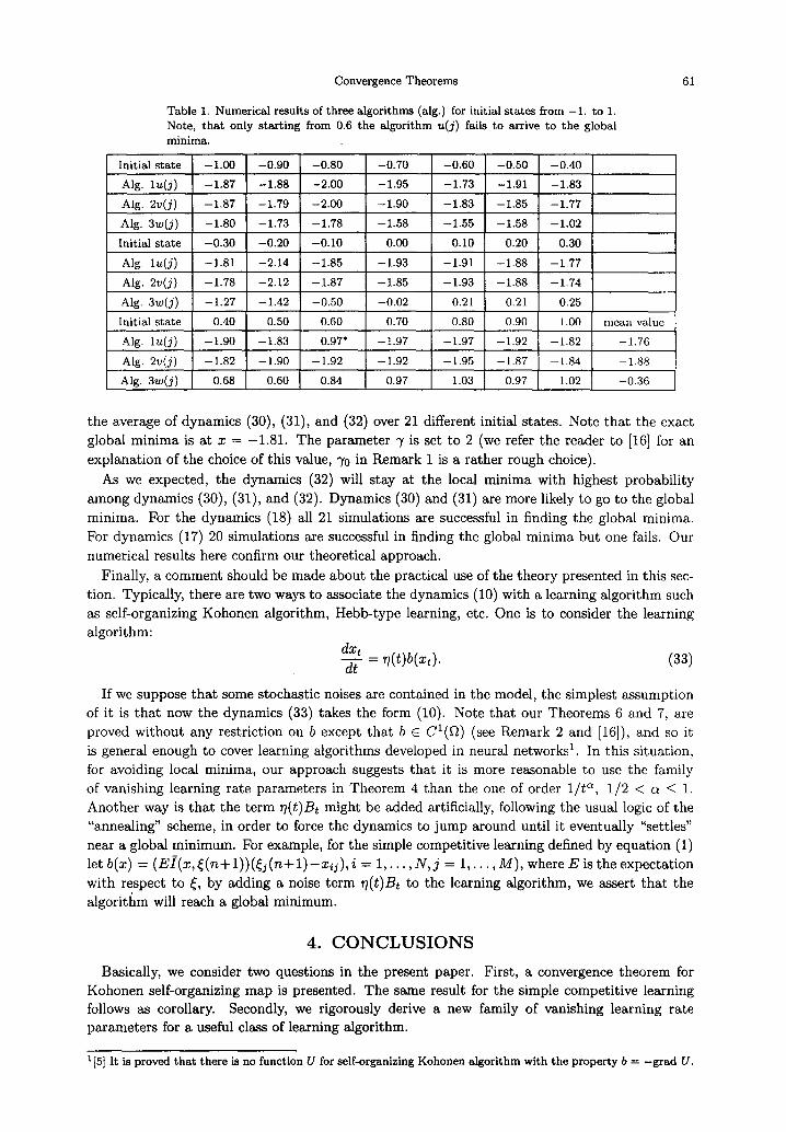
Table 1. Numerical results of three algorithms (alg.) for initial states from -1. to 1. Note, that only starting from 0.6 the algorithm u(j) fails to arrive to the global minima.

Initial state -1.00

hlg. lu(j) -1.87

Alg. 2v(j) -1.87

Alg. 3w(j) --1.80

Initial state -0.30

hlg. lu(j) -1.81

Alg. 2v(j) -1.78

Alg. 3w(j) -1.27

Initial state 0.40

hlg. lu(j) -1.90

hlg. 2v(j) -1.82

Alg. 3w(j) 0.68

-0.90

- 1 . 8 8

-1.79

-1.73

-0.20

-2.14

-2.12

-1.42

0.50

-1.83

-1.90

0.60

-0.80 -0.70

-2.00 -1.95

-2.00 - 1.90

-1.78 -1.58

-0.10 0.00

-1.85 -1.93

-1.87 -1.85

-0.50 -0.02

0.60 0.70

0.97* -1.97

-1.92 -1.92

0.84 0.97

--0.60 -0.50 -0.40

-1.73 -1.91 --1.83

-1.83 -1.85 --1.77

--1.55 - -1 .58 --1.02

0.10 0.20 0.30

-1.91 -1.88 --1.77

-1.93 -1.88 -1.74

0.21 0.21 0.25

0.80 0.90 1.00

-1.97 -1.92 -1.82

-1.95 -1.87 -1.84

1.03 0.97 1.02

mean value

-1.76

-1.88

--0.36

61

the average of dynamics (30), (31), and (32) over 21 different initial states. Note that the exact

global minima is at x = -1.81. The parameter 7 is set to 2 (we refer the reader to [16] for an

explanation of the choice of this value, 70 in Remark 1 is a rather rough choice).

As we expected, the dynamics (32) will stay at the local minima with highest probability

among dynamics (30), (31), and (32). Dynamics (30) and (31) are more likely to go to the global

minima. For the dynamics (18) all 21 simulations are successful in finding the global minima.

For dynamics (17) 20 simulations are successful in finding the global minima but one fails. Our

numerical results here confirm our theoretical approach.

Finally, a comment should be made about the practical use of the theory presented in this sec-

tion. Typically, there are two ways to associate the dynamics (10) with a learning algorithm such

as self-organizing Kohonen algorithm, Hebb-type learning, etc. One is to consider the learning algorithm:

dxt d~ = ~(t)b(xt). (33)

If we suppose that some stochastic noises are contained in the model, the simplest assumption

of it is that now the dynamics (33) takes the form (10). Note that our Theorems 6 and 7, are

proved without any restriction on b except that b E C1(~) (see Remark 2 and [16]), and so it

is general enough to cover learning algorithms developed in neural networks 1. In this situation, for avoiding local minima, our approach suggests that it is more reasonable to use the family

of vanishing learning rate parameters in Theorem 4 than the one of order 1/t ~, 1/2 < a < 1.

Another way is that the term ~?(t)Bt might be added artificially, following the usual logic of the "annealing" scheme, in order to force the dynamics to jump around until it eventually "settles"

near a global minimum. For example, for the simple competitive learning defined by equation (1) let b(x) = (ET_(x, ~ ( n + l ) ) ( ~ j ( n + l ) - x ~ j ) , i = 1 , . . . , g , j = 1 . . . . , M) , where Z is the expectation

with respect to ~, by adding a noise term ~(t)Bt to the learning algorithm, we assert that the

algorithm will reach a global minimum.

4. C O N C L U S I O N S

Basically, we consider two questions in the present paper. First, a convergence theorem for

Kohonen self-organizing map is presented. The same result for the simple competitive learning follows as corollary. Secondly, we rigorously derive a new family of vanishing learning rate parameters for a useful class of learning algorithm.

1 [5] It is proved that there is no function U for self-organizing Kohonen algorithm with the property b = -grad U.

62 J , F. FENG AND B. TIROZZ!

Global optimization of learning in neural networks is currently an important subject. How can one be sure that the learning network reaches the optimal state, i.e., the global minimum of some error criterion, and does not get stuck in a local minimum? A well known strategy to find the global minimum and not just a local minimum is simulated annealing [16], a noise parameter, say temperature, is cooled down slowly. More specifically, we consider the following stochastic differential equation (or Langevin equation)

dXt = -g rad U(X t ) dt + a( t ) dBt , (34)

and when

we have

- 7 /log(t + 2) ' (35)

lim P(XtEA)=I, t ---~OO

where A is the set of global minima of U, and 7 is a constant depending on U. Learning in neural networks such as self-organizing Kohonen algorithm, Hebb learning, etc.,

are also a stochastic process. At each learning step, a training pattern is drawn at random from the environment (the total set of training patterns) and presented to the network. A large learning parameter leads to large fluctuations in the synaptic weight of the network. So, in a way, the learning parameter can be viewed as a noise parameter akin to the temperature in simulated annealing. A typical case of such learning algorithms (see, final chapter, of previous section) is

dYt = rl(t) (b(Yt) dt + l~(t) dBt ) , (36)

a dynamics studied in stochastic approximation theory for many years. Note that when b = -g rad U, rl(t) = 1, and c~(t) = j3(t) we have Xt = Yt, and thus, the case for simulated annealing is just a special case of (36).

In the present paper, we derive a family of vanishing learning rate parameters based upon a rigorous analysis on (36) and our previous results of simulated annealing in [16]. The new family of vanishing learning rate parameters satisfy the following condition

o ~ ~(u) du = c~,

7

~(t) = t) fo rl(U) du

(37)

which in general violates the condition (10) found in stochastic approximation theory. Again we want to point out here that when r/(u) = 1, the rate (22) found in simulated annealing algorithm defined by (34) is exactly a special case of our results here.

Finally, we like to comment on further possible developments of our results here. Obviously a case to case and systematic numerical simulations for algorithms developed in neural networks with VLRPs in Theorem 6 and Theorem 7, are quite interesting and is one of our further topics. Theoretically simulated annealing of form (34) has been well studied [16] and on the other hand stochastic approximation theory taking into account the dynamics (36) has developed into a mature field already. In particular, many estimates on convergence rate (in neural networks, convergence rate is called learning error and generalization error) for both algorithms have been established already. We believe that the method developed in this paper serves as a bridge between these two fields and will help us to understand more deeply the behavior of learning algorithms in neural networks and may provide a theoretical basis for the design of practical algorithms that lead to global optimization of learning in neural networks.

Convergence Theorems 63

R E F E R E N C E S 1. S. Albeverio, N. Kriiger and B. Tirozzi, An extension of Kohonen phonetic maps for speech recognition,

Mathl. Comput. Modelling (to appear). 2. D. Amit, Modeling Brain Function, Cambridge Univ. Press, (1989). 3. J.A. Hertz, A. Krogh and R. Palmer, Introduction to the Theory of Neural Computation, Addison-Wesley,

Redwood City, CA, (1991). 4. E. Erwin, K. Obermayer and K. Schulten, Self-organizing maps: Stationary states, metastability and conver-

gence rate, Biol. Cybern. 67, 35-45, (1992). 5. E. Erwin, K. Obermayer and K. Schulten, Self-organizing maps: Ordering, convergence properties and energy

functions, Biol. Cybern. 67, 47-55, (1992). 6. C. Bouton and G. PagES, Self-organization and convergence of the one-dimensional Kohonen algorithm with

non uniformly distributed stimuli, Stoch. Proc. Appl. 47, 249-274, (1993). 7. C. Bouton and G. PagEs, Convergence in distribution of the one-dimensional Kohonen algorithms when the

stimuli are not uniform, Adv. Appl. Prob. 26, 80-103, (1994). 8. M. Cottrell and J.C. Fort, Etude d'un algorithme d'auto-organisation, Ann. Inst. H. Poincard 23, 1-20,

(1986). 9. T. Martinetz and K. Schulten, Topology representing networks, Neural network 7, 507-522, (1994).

10. A. Benveniste, M. Mdtivier and P. Priouret, Adaptive Algorithms and Stochastic Approximations, Springer- Verlag, Berlin, (1990).

11. P. Hall and C.C. Heyde, Martingale Limit Theory and its Application, Academic Press, New York, (1980). 12. T. Kohonen, Self-Organization and Associative Memory, 3 rd Edition, Springer-Verlag, Berlin, (1989). 13. H. Kushner and D. Clark, Stochastic Approximation Methods for Constrained and Unconstrained Systems,

Springer-Verlag, New York, (1978). 14. M.B. Nevel'son and R.Z. Has'minskii, Stochastic Approximation and Recursive Estimation, Translation of

Math. Monograph 47, Amer. Math. Soc., Providence, RI, (1976). 15. H. Ritter, T. Martinetz and K. Schulten, Neural Computation and Self-Organizing Maps, Addison-Wesley,

Reading, MA, (1992). 16. S. Albeverio, J.F. Feng and M.P. Qian, Role of noises in neural networks, Phys. Rev. E 52, 6593-6606, (1995). 17. J.F. Feng, H. Pan and V.P. Roychowdhury, On neurodynamics with limiter function and Linsker's develop-

mental model, Neural Computation 8, 1003-1019, (1996). 18. S. Amari, Information geometry of the EM and em algorithms for neural network, Neural Networks 8,

1379-1408, (1995). 19. G.J. Goodhill, Topography and ocular dominance:a model exploring positive correlations, Bio. Cyber. 69,

109-118, (1993). 20. G.J. Goodhill and D.J. Willshaw, Elastic net model of ocular dominance: Overall stripe pattern and monoc-

ular deprivation, Neural Computation 6, 615-621, (1994). 21. J.F. Feng and B. Tirozzi, A discrete version of the dynamic link network, Neurocomputing 14 (to appear). 22. M. Lades, J.C. Vorbriiggen, J. Buhrmann, J. Lange, C. von der Malsburg, R.P. Wfirtz and W. Konen,

Distortion invariant object recognition in the dynamic link architecture, IEEE Transactions on Computers 42, 300-311, (1993).

23. C. Bishop, Neural Networks for Pattern Recognition, Oxford University Press, (1995). 24. J.F. Feng and M.P. Qian, Two-stage annealing in retrieving memories I, In Probability and Statistics, (Edited

by A. Badrikian, P.-A. Meyer and J.-A. Yan), pp. 149-176, World Scientific, Singapore, (1993). 25. M.I. Freidlin and A.D. Wentzell, Random Perturbations o/Dynamic System, Springer-Verlag, Berlin, (1984). 26. S.Y. Chow and H. Teicher, Probability Theory, Springer-Verlag, New York, (1988).