convergence analysis of multi delity monte carlo...
TRANSCRIPT

Noname manuscript No.(will be inserted by the editor)
Convergence analysis of multifidelity Monte Carloestimation
Benjamin Peherstorfer · MaxGunzburger · Karen Willcox
Received: date / Accepted: date
Abstract The multifidelity Monte Carlo method provides a general frame-work for combining cheap low-fidelity approximations of an expensive high-fidelity model to accelerate the Monte Carlo estimation of statistics of thehigh-fidelity model output. In this work, we investigate the properties of mul-tifidelity Monte Carlo estimation in the setting where a hierarchy of approx-imations can be constructed with known error and cost bounds. Our mainresult is a convergence analysis of multifidelity Monte Carlo estimation, forwhich we prove a bound on the costs of the multifidelity Monte Carlo es-timator under assumptions on the error and cost bounds of the low-fidelityapproximations. The assumptions that we make are typical in the setting ofsimilar Monte Carlo techniques. Numerical experiments illustrate the derivedbounds.
Keywords multifidelity · multilevel · hierarchical methods · Monte Carlo ·surrogates · coarse-grid approximations · partial differential equations withrandom coefficients · uncertainty quantification
B. PeherstorferDepartment of Mechanical Engineering and Wisconsin Institute for Discovery, University ofWisconsin-Madison, Madison, WI 53706E-mail: [email protected]
M. GunzburgerDepartment of Scientific Computing, Florida State University, 400 Dirac Science Library,Tallahassee FL 32306-4120E-mail: [email protected]
K. WillcoxDepartment of Aeronautics & Astronautics, MIT, Cambridge, MA 02139E-mail: [email protected]

2 1 INTRODUCTION
1 Introduction
Inputs to systems are often modeled as random variables to account for theuncertainties in the inputs due to inaccuracies and incomplete knowledge.Given the input random variable and a model of the system of interest, animportant task is to estimate statistics of the model output random variable.
Monte Carlo estimation is one popular approach to estimate statistics. Ba-sic Monte Carlo estimation generates samples of the input random variable,discretizes the model and then solves the discretized model—the high-fidelitymodel—up to the required accuracy at these samples, and averages over thecorresponding outputs to estimate statistics of the model output random vari-able. This basic Monte Carlo estimation often requires many samples, andconsequently many approximations of the model outputs, which can becometoo costly if the high-fidelity model solves are expensive. We note that othertechniques than Monte Carlo estimation are available to estimate statistics ofmodel outputs, see, e.g., [1,33,21,15,14,47,43,45].
Several variance reduction techniques have been presented to reduce thecosts of Monte Carlo simulation compared to basic Monte Carlo estimators,e.g., antithetic variates [39,23,28] and importance sampling [39,27,36]. Ourfocus here is on the control variate framework that exploits the correlationbetween the model output random variable and an auxiliary random vari-able that is cheap to sample [30]. A major class of control variate methodsderives the auxiliary random variable from cheap approximations of the out-puts of the high-fidelity model. For example, in situations where the model isgoverned by (often elliptic) partial differential equations (PDEs), coarse-gridapproximations of the PDE—low-fidelity models—can provide cheap approx-imations of the outputs obtained from a fine-grid high-fidelity discretizationof the PDE; however, other types of low-fidelity models are possible in thecontext of PDEs, e.g., projection-based reduced models [41,40,20,3,37], data-fit interpolation and regression models [13,12], machine-learning-based modelssuch as support vector machines [46,11], and other simplified models [29,32].
The multifidelity Monte Carlo (MFMC) method [38] uses a control variateapproach to combine auxiliary random variables stemming from low-fidelitymodels into an estimator of the statistics of the high-fidelity model output.Key to the MFMC approach is the selection of how often each of the auxiliaryrandom variables is sampled, and therefore how often each of the low-fidelitymodels is solved. The MFMC approach derives this selection from the correla-tion coefficients between the auxiliary random variables and the high-fidelitymodel output random variable. The selection of the MFMC approach is opti-mal in the sense that the variance of the MFMC estimator is minimized forgiven maximal costs of the estimation. We refer to the discussions in [38,31]for details on MFMC.
The work [38] discusses the properties of MFMC estimation in a settingwhere only mild assumptions on the high- and low-fidelity models are made.We consider here the setting where we can make further assumptions on theerrors and costs of outputs obtained with a hierarchy of low- and high-fidelity

3
models. Our contribution is to show that for an MFMC estimator with mean-squared error (MSE) below a threshold parameter ε > 0, the costs of theestimation can be bounded by ε−1 up to a constant under certain conditionson the error and cost bounds of the models in the hierarchy.
We discuss that the conditions we require in the MFMC context are similarto the conditions exploited by the multilevel Monte Carlo method [9, Theo-rem 1]. Our analysis shows that MFMC estimation is as efficient in terms oferror and costs as multilevel Monte Carlo estimation under certain conditionsthat we discuss below in detail. Multilevel Monte Carlo uses a hierarchy oflow-fidelity models—typically coarse-grid approximations—to derive a hierar-chy of auxiliary random variables, which are combined in a judicious way toreduce the runtime of Monte Carlo simulation. Multilevel Monte Carlo was in-troduced in [26] and extended and made popular by the work [18]. Since then,the properties of the multilevel Monte Carlo estimators have been studied ex-tensively in different settings, see, e.g., [9,8,2,6,42]. Multilevel Monte Carloand its variants have also been applied to density estimation [5], variance es-timation [4], and rare event simulation [44]. We also mention the continuationmultilevel Monte Carlo [10] and the extension multi-index Monte Carlo thatallows different mesh widths in the dimensions [22]. In [34,35], a fault-tolerantmultilevel Monte Carlo is introduced and analyzed, which is well suited formassively parallel computations. An integer optimization problem is solvedto determine the optimal number of model evaluations depending on the rateof compute-node failures. The fault-tolerant approach thus takes into accountnode failure by adapting the number of model evaluations accordingly. Therelationship between multilevel Monte Carlo and sparse grid quadrature [7,16,17] is discussed in [24,25,19].
The outline of the presentation is as follows. Section 2 introduces the prob-lem setup and basic, multilevel, and multifidelity Monte Carlo estimators. Sec-tion 3 derives the new convergence analysis of MFMC estimation. Numericalexamples in Section 4 illustrate the derived bounds. Conclusions are drawn inSection 5.
2 Problem setup
This section introduces the problem setup and the various types of Monte Carloestimators required throughout the presentation. Section 2.1 introduces thenotation and Section 2.2 the basic Monte Carlo estimator. Multilevel MonteCarlo and the MFMC estimation are summarized in Section 2.3 and Sec-tion 2.4, respectively.
2.1 Preliminaries
The set of positive real numbers is denoted as R+ = x ∈ R : x > 0. Fortwo positive quantities a and b, we define a . b to hold if a/b is bounded by

4 2 PROBLEM SETUP
a constant whose value is independent of any parameters on which a and bdepend on.
Let d ∈ N be the dimension and define the Lipschitz domain D ⊂ Rd. LetZ : Ω → D be a random variable over a probability space (Ω,F ,P), whereΩ denotes the set of outcomes, F the σ-algebra of events, and P : F → [0, 1]a probability measure. Let further Q : D → R be a function in a suitablefunction space and let Q` : D → R be functions for ` ∈ N that approximate Qin the sense of the following assumption. Note that we assume that Q(Z) andQ`(Z) are integrable.
Assumption 1 There exists 1 < s ∈ R and rate α ∈ R+ such that
|E[Q(Z)−Q`(Z)]| ≤ κ1s−α` , ` ∈ N ,
where κ1 ∈ R+ is a constant independent of `.
The parameter ` ∈ N is the level of Q`. Let further w` ∈ R+ be the costs ofevaluating Q` for ` ∈ N. The following assumption gives a bound on the costswith respect to the level `.
Assumption 2 There exists a rate γ ∈ R+ with
w` ≤ κ3sγ` ,
where the constant s is given by Assumption 1 and κ3 ∈ R+ is a constantindependent of `.
Note that in Assumption 2 the same constant s as in Assumption 1 is used.The variance Var[Q`(Z)] of the random variable Q`(Z) is denoted as
σ2` = Var[Q`(Z)] , ` ∈ N .
We make the assumption that there exists a positive lower and upper boundfor the variance σ2
` with respect to level ` ∈ N.
Assumption 3 There exist σlow ∈ R+ and σup ∈ R+ such that σlow ≤ σ` ≤σup for ` ∈ N.
The Pearson product-moment correlation coefficient of the random variablesQ`(Z) and Ql(Z) is denoted as
ρ`,l =Cov[Q`(Z), Ql(Z)]
σ`σl, `, l ∈ N , (1)
where Cov[Q`(Z), Ql(Z)] is the covariance of Q`(Z) and Ql(Z).We consider the situation where the random variable Z represents an input
random variable and Q is a function that maps an input, i.e., a realizationof Z, onto an output. In our situation, evaluating Q entails solving a PDE(“model”), but the solutions to the PDE are unavailable. We therefore revert tosolving an approximate PDE (“discretized model”), where the approximation(e.g., the mesh width) is controlled by the level `. The functions Q` map the

2.2 BASIC MONTE CARLO ESTIMATION 5
input onto the output obtained by solving the approximate PDE on level `.Assumption 1 specifies in which sense Q` converges to Q with `→∞. Solvingthe approximate PDE on level ` incurs costs w`. One task in this context is toderive estimators of E[Q(Z)] using the functions Q`. We assess the efficiency
of an estimator Q with its MSE
e(Q) = E[(Q− E[Q(Z)]
)2],
and its costs c(Q), which are the sum of the evaluation costs w` of the functions
Q` used in the estimator Q. An estimator Q with MSE e(Q) . ε below a
threshold ε ∈ R+ is efficient, if the costs c(Q) . ε−1 are bounded by ε−1 up toa constant. Note that ε bounds the MSE, in contrast to the root-mean-squarederror (RMSE) as in, e.g., [9].
2.2 Basic Monte Carlo estimation
Let ` ∈ N and define the basic Monte Carlo estimator QMC`,m of E[Q`(Z)] as
QMC`,m =
1
m
m∑i=1
Q`(Zi) ,
with m ∈ N independent and identically distributed (i.i.d.) samples Z1, . . . , Zmof Z. The MSE of the Monte Carlo estimator QMC
`,m with respect to E[Q(Z)] is
e(QMC`,m) = m−1 Var[Q`(Z)] + (E[Q(Z)−Q`(Z)])
2. (2)
The term m−1 Var[Q`(Z)] is the variance term and term (E[Q`(Z)−Q(Z)])2
is the bias term. The costs of the estimator QMC`,m are
c(QMC`,m) = mw` ,
because Q` is evaluated at m samples, with one evaluation having costs w`.Let now ε ∈ R+ be a threshold. One approach to obtain a basic Monte
Carlo estimator QMC`,m with e(QMC
`,m) . ε is to derive a maximal level L ∈ N anda number of samples m such that the bias and the variance term are boundedby ε/2 up to constants. Consider first the choice of the maximal level L ∈ N.With Assumption 1, the maximal level L is given by
L =⌈α−1 logs
(√2κ1ε
−1/2)⌉
, (3)
where κ1 is the constant in Assumption 1. Note that the maximal level Ldefines the high-fidelity model QL in the terminology of the introduction, seeSection 1.
To achieve that the variance term is bounded by ε/2 up to a constant, thenumber of samples m is selected such that ε−1 . m. With Assumption 2, and

6 2 PROBLEM SETUP
assuming the variance σ2` is approximately constant with respect to the level
`, the costs of the basic Monte Carlo estimator QMCL,m are
c(QMCL,m) . ε−1−γ/(2α) ,
see [9, Section 2.1] for a proof. The costs of the basic Monte Carlo estimatorscale with the rates γ and α.
2.3 Multilevel Monte Carlo estimation
We follow [9] for the presentation of the multilevel Monte Carlo estimation.Consider the threshold ε ∈ R+ and define the maximal level L ∈ N as in (3).Multilevel Monte Carlo exploits the linearity of the expected value to write
E[QL(Z)] = E[Q1(Z)] +
L∑`=2
E[Q`(Z)−Q`−1(Z)] =
L∑`=1
E[∆`(Z)] ,
where ∆`(Z) = Q`(Z) − Q`−1(Z) for ` > 1 and ∆1(Z) = Q1(Z). The basicMonte Carlo estimator of ∆`(Z) with m` ∈ N samples Z1, . . . , Zm` is
∆MC`,m`
=1
m`
m∑i=1
Q`(Zi)−Q`−1(Zi) .
The multilevel Monte Carlo estimator QMLL,m is then given by
QMLL,m =
L∑`=1
∆MC`,m`
, (4)
where the vector m = [m1, . . . ,mL]T ∈ NL is the vector of the number of
samples at each level. Note that each basic Monte Carlo estimator ∆MC`,m`
in(4) uses a separate, independent set of samples. Note further that the functionsQ1, . . . , QL−1 are low-fidelity models in the terminology of the introduction,see Section 1.
Under the following two assumptions, and with a judicious choice of thenumber of samples m, the multilevel Monte Carlo estimator is efficient, whichmeans that the estimator QML
L,m achieves an MSE of e(QMLL,m) . ε with costs
c(QMLL,m) . ε−1. The first assumption states that the variance of ∆` decays
with the level `.
Assumption 4 There exists a rate β ∈ R+ with
Var[Q`(Z)−Q`−1(Z)] ≤ κ2s−β` , ` ∈ N ,
where s is the constant of Assumption 1 and κ2 ∈ R+ is a constant independentof `.

2.4 MULTIFIDELITY MONTE CARLO ESTIMATION 7
The following assumption sets the rate β of the decay of the variance Var[Q`(Z)−Q`−1(Z)] in relation to the rate γ of the increase of the costs with level `.
Assumption 5 For the rates γ of Assumption 2 and β of Assumption 4, wehave β > γ.
Set the number of samples mML = [mML1 , . . . ,mML
L ]T to
mML` =
⌈2ε−1κ2
(1− s−(β−γ)/2
)−1s−(β+γ)`/2
⌉, ` = 1, . . . , L , (5)
where κ2 is the constant in Assumption 4 and s is defined as in Assump-tion 1. Note that the components of mML are rounded up. It is shown in[9] that if Assumptions 1–5 hold, then the multilevel Monte Carlo estimator
QMLL,mML with mML defined in (5) achieves an MSE of e(QML
L,mML) . ε with
costs c(QMLL,mML) . ε−1. Note that under Assumptions 1–5 it is sufficient to
select the number of samples with the rates β and γ to achieve an efficientestimator. We refer to [26,18,9] for details on multilevel Monte Carlo estima-tion.
2.4 Multifidelity Monte Carlo estimation
The MFMC estimator [38] uses functions Q1, . . . , QL up to the maximal levelL to derive an estimate of E[Q(Z)], similarly to the multilevel Monte Carloestimator; however, the functions Q1, . . . , QL are combined in a different waythan in the multilevel Monte Carlo estimator, and the number of samples mare selected by directly using correlation coefficients and costs instead of rates.
MFMC imposes on the number of samples m = [m1, . . . ,mL]T that m1 ≥m2 ≥ · · · ≥ mL > 0. Let
Z1, . . . , Zm1 ∈ D (6)
be m1 i.i.d. samples of the random variable Z. Let further
Q`(Z1), . . . , Q`(Zm`) , (7)
be the evaluations of Q` at the first m` samples Z1, . . . , Zm` , for ` = 1, . . . , L.Consider now the basic Monte Carlo estimators
QMC`,m`
=1
m`
m∑i=1
Q`(Zi) , ` = 1, . . . , L , (8)
and
QMC`,m`+1
=1
m`+1
m`+1∑i=1
Q`(Zi) , ` = 1, . . . , L− 1 , (9)
which use the samples (6) and the evaluations (7). Note that the estimators in
(9) use the first m`+1 samples of the samples (6). Thus, the estimators QMC`,m`

8 2 PROBLEM SETUP
and QMC`,m`+1
are dependent for ` = 1, . . . , L− 1. The MFMC estimator QMFL,m
is defined as
QMFL,m = QMC
L,mL +
L−1∑`=1
a`
(QMC`,m`− QMC
`,m`+1
),
where a = [a1, . . . , aL−1]T ∈ RL−1 are coefficients. The costs of the MFMC
estimator QMFL,m are
c(QMFL,m) = wTm ,
where w = [w1, . . . , wL]T , see [38].The MFMC method provides a framework to select the number of samples
m and the coefficients a such that the variance Var[QMFL,m] of the MFMC
estimator QMFL,m with costs c(QMF
L,m) = p is minimized for a given computationalbudget p ∈ R+. The number of samples m and the coefficients a are derivedunder two assumptions on the correlation coefficients of Q1(Z), . . . , QL(Z)and the costs w1, . . . , wL. The first assumption specifies the ordering of thefunctions Q1(Z), . . . , QL(Z).
Assumption 6 The random variables Q1(Z), . . . , QL(Z) are ordered ascend-ing with respect to the absolute values of the correlation coefficients
|ρL,1| < |ρL,2| < · · · < |ρL,L| .
The second assumption describes inequalities of the correlation coefficients andthe costs.
Assumption 7 The costs w1, . . . , wL and correlation coefficients ρL,1, . . . , ρL,Lsatisfy
w`+1
w`>ρ2L,`+1 − ρ2L,`ρ2L,` − ρ2L,`−1
for ` = 1, . . . , L− 1.
Assumption 7 enforces that the cost savings associated with a model justify itsdecrease in accuracy (measured by correlation) relative to other models in thehierarchy. If a particular model violates the condition in Assumption 7, theMFMC method omits the model from the hierarchy. See [38] for more details.
Under Assumptions 6–7, the number of samples m and the coefficients a,which minimize the variance of Var[QMF
L,m] with costs c(QMFL,m) = p, are given
as follows [38]. The coefficients aMF = [aMF1 , . . . , aMF
L−1]T are set to
aMF` =
ρL,`σLσ`
, ` = 1, . . . , L− 1 ,
and the number of samples mMF = [mMF1 , . . . ,mMF
L ]T is set to
mMF` = mMF
L r` , ` = 1, . . . , L ,

9
where
r` =
√wL(ρ2L,` − ρ2L,`−1)
w`(1− ρ2L,L−1), ` = 1, . . . , L , (10)
with ρL,0 = 0. Note that the selection of mMF and aMF is independent of therates α, β, γ, which means the approach is applicable also in situations whererates capture the behavior of the properties of the functions Q1, . . . , QL onlypoorly, see, e.g., [38] for examples. Note further that the components of thenumber of samples mMF are rounded up to integer numbers as in the mul-tilevel Monte Carlo method, see (5) in Section 2.3. We note that in [34] aninteger optimization problem is solved to adapt the number of model evalua-tions in multilevel Monte Carlo for an increased processor-failure tolerance onmassively-parallel compute platforms.
The MFMC estimator is unbiased with respect to E[QL(Z)], see [38, Lemma 3.1].
The variance of the MFMC estimator QMFL,mMF is [38]
Var(QMFL,mMF) =
σ2L(1− ρ2L,L−1)(mMFL
)2wL
p .
The work [38] investigates the costs and the MSE of the MFMC estimator onlyin the context of Assumption 6 and Assumption 7, and does not give insightsinto the behavior of the MFMC estimator if additionally Assumptions 1–5 aremade.
3 New properties of the multifidelity Monte Carlo estimator
We now discuss the error and costs behavior of the MFMC estimator in atypical setting of the multilevel Monte Carlo estimators where Assumption 4on the rate of the variance decay and Assumption 5 on the relative costs hold.Our main result is Theorem 1 that states that the MFMC estimator is efficientunder Assumptions 1–7, which means that the MFMC estimator achieves anMSE e(QMF
L,mMF) . ε with costs c(QMFL,mMF) . ε−1, independent of the rates α
and γ. We first state Theorem 1 and then prove two lemmata in Section 3.1and provide the proof of Theorem 1 in Section 3.2. Corollary 1 discusses theconvergence rates of MFMC if Assumption 5 is violated.
Theorem 1 With Assumptions 1–5, as well as Assumption 6 and Assump-tion 7, set the maximum level L as in (3) and set the budget p to
p = κ4ε−1 , (11)
with the constant
κ4 = 2σ2up
σ2low
(sγ−β
2
1− s γ−β2
)2
.

103 NEW PROPERTIES OF THE MULTIFIDELITY MONTE CARLO
ESTIMATOR
For the number of samples mMF and the coefficients aMF ∈ RL−1 defined inSection 2.4, the MSE e(QMF
L,mMF) of the MFMC estimator with respect to the
statistics E[Q(Z)] is bounded as
e(QMFL,mMF) . ε ,
and the costs are bounded as c(QMFL,mMF) . ε−1.
Note that the MLMC theory developed in [9, Theorem 1] and [18, Theo-rem 3.1] requires an additional assumption on the rate α because the roundingup of the numbers of samples to an integer is explicitly taken into account, seealso [4, Theorem 3.2]. We ignore the rounding here and therefore can avoidthat assumption; however, we emphasize that we expect that a similar as-sumption is necessary for MFMC as well if the rounding of the numbers ofsamples is taken into account explicitly.
3.1 Preliminary lemmata
This section proves two lemmata that we use in the proof of Theorem 1 inSection 3.2.
Lemma 1 Let L ∈ N be the maximal level. From Assumption 4, it followsthat
Var[QL(Z)−Q`−1(Z)] . s−β` , (12)
for ` = 2, . . . , L− 1.
Proof Let κ2 be the constant in Assumption 4 so that we have
Var[Q`(Z)−Q`−1(Z)] ≤ κ2s−β` ,
for ` ∈ N. We obtain
Var[Q`+1(Z)−Q`−1(Z)] ≤ Var[Q`+1(Z)−Q`(Z)] + Var[Q`(Z)−Q`−1(Z)]
+ 2|Cov[Q`+1(Z)−Q`(Z), Q`(Z)−Q`−1(Z)]| . (13)
With Assumption 4 and the Cauchy-Schwarz inequality, it follows that
Var[Q`+1(Z)−Q`−1(Z)] ≤ κ2s−β(`+1) + κ2s−β`
+ 2√
Var[Q`+1(Z)−Q`(Z)] Var[Q`(Z)−Q`−1(Z)] ,
and therefore we have
Var[Q`+1(Z)−Q`−1(Z)] ≤κ2s−β(`+1) + κ2s−β` + 2κ2s
−β(2`+1)/2
≤κ2s−β`(s−β + 1 + 2s−β/2)
≤κ2s−β`(s−β/2 + 1 + 2s−β/2) ,
(14)

3.1 PRELIMINARY LEMMATA 11
where the last inequality holds because s > 1. Define now the sequence (bj)with
b0 = 1 , bj = s−βj/2 + bj−1(1 + 2s−βj/2) , j ∈ N .
From (14) and from the definition of the sequence (bj), it follows with inductionthat
Var[Q`+j(Z)−Q`−1(Z)] ≤κ2s−β(`+j) + κ2bj−1s−β` + 2κ2s
−β`(bj−1s−βj)1/2
≤κ2s−β`(s−βj + bj−1 + 2(bj−1s−βj)1/2)
≤κ2s−β`(s−βj + bj−1 + 2bj−1s−βj/2)
≤κ2s−β`(s−βj/2 + bj−1(1 + 2s−βj/2))
≤κ2s−β`bj ,
because bj ≥ 1 (and therefore b1/2j ≤ bj) and s > 1 for j ∈ N. To bound the
sequence (bj), rewrite
bj =
j∑i=0
s−βi/2j∏
r=i+1
(1 + 2s−βr/2) ,
and observe that
j∏r=i+1
(1 + 2s−βr/2) ≤∞∏r=0
(1 + 2s−βr/2) .
The infinite product converges if and only if the series
∞∑r=0
2s−βr/2
converges, which is the case because s > 1 and therefore s−β/2 < 1. Denote
∞∏r=0
(1 + 2s−βr/2) = κ5 ,
with the constant κ5 ∈ R, and obtain the bound κ6 ∈ R
bj ≤ κ5j∑i=0
s−βi/2 ≤ κ6 , j ∈ N .
Using bj ≤ κ6 and (14) shows the lemma.
Lemma 2 From Assumption 4, Assumption 3, and Lemma 1, it follows that
ρ2L,` − ρ2L,`−1 .1
σ2low
s−β` .

123 NEW PROPERTIES OF THE MULTIFIDELITY MONTE CARLO
ESTIMATOR
Proof First, we ensure ρL,` ≥ 0 for ` ∈ N w.l.o.g. by redefining Q` to −Q`if necessary, and subsequently using −Q` in the estimators (8) and (9). Withthe definition of the correlation coefficient (1), we obtain
0 ≤ ρL,` − ρL,`−1 =ρL,` −Cov[QL(Z), Q`−1(Z)]
σLσ`−1
=ρL,` −1
σLσ`−1Cov[QL(Z), Q`−1(Z)] +
1
2
σ2L
σLσ`−1− 1
2
σ2L
σLσ`−1
+1
2
σ2`−1
σLσ`−1− 1
2
σ2`−1
σLσ`−1
=ρL,` +1
2σLσ`−1Var[QL(Z)−Q`−1(Z)]− 1
2
(σLσ`−1
+σ`−1σL
),
(15)
where we used
Var[QL(Z)−Q`−1(Z)] = Var[QL(Z)]+Var[Q`−1(Z)]−2 Cov[QL(Z), Q`−1(Z)] .
With x = σL/σ`−1, we can rewrite the last term in (15) as
1
2
(σLσ`−1
+σ`−1σL
)=
1
2
(x+
1
x
).
Because
1
2
(x+
1
x
)≥ 1
holds for x ∈ R+, and because 0 ≤ ρL,` ≤ 1 per definition, we obtain thefollowing bound on ρL,` − ρL,`−1
0 ≤ ρL,` − ρL,`−1 =ρL,` +1
2σLσ`−1Var[QL(Z)−Q`−1(Z)]− 1
2
(σLσ`−1
+σ`−1σL
)≤ 1
2σLσ`−1Var[QL(Z)−Q`−1(Z)]
.1
σ2low
s−β` ,
where we used Lemma 1 to bound Var[QL(Z)−Q`−1(Z)] and the lower boundσlow of Assumption 3. Since ρL,` + ρL,`−1 ≤ 2, we obtain
ρ2L,` − ρ2L,`−1 = (ρL,` − ρL,`−1)(ρL,` + ρL,`−1) .1
σ2low
s−β` .

3.2 PROOF OF MAIN THEOREM 13
3.2 Proof of main theorem
With the Lemmata 1–2 discussed in Section 3.1, we now prove Theorem 1.
Proof (of Theorem 1) The MSE of the MFMC estimator QMFL,mMF is split into
the biasing and the variance term
e(QMFL,mMF) = Var[QMF
L,mMF ] + (E[Q(Z)−QL(Z)])2. (16)
We first consider the biasing term of the MSE. With the maximal level Ldefined as in (3), we obtain with Assumption 1
(E[Q(Z)−QL(Z)])2 .
ε
2.
Consider now the variance term Var[QMFL,mMF ]. Assumption 3 means that σ` ≤
σup for ` = 1, . . . , L. We therefore have
Var[QMFL,mMF ] ≤
σ2up
(1− ρ2L,L−1
)(mMFL
)2wL
p =σ2up
(1− ρ2L,L−1
)pwL
(L∑`=1
w`r`
)2
,
where we used mMFL = p/(wTr) and r = [r1, . . . , rL]T defined in (10) in
Section 2.4. Note that Assumptions 6–7 are required for mMF and aMF to beoptimal in the sense defined in Section 2.4. We further have with the definitionof r in (10) in Section 2.4 that
σ2up
(1− ρ2L,L−1
)pwL
(L∑`=1
w`r`
)2
=σ2up
p
(L∑`=1
√w`
(ρ2L,` − ρ2L,`−1
))2
, (17)
see [38, Proof of Corollary 3.5] for the transformations. With Assumption 2and Lemma 2, we obtain
L∑`=1
√w`
(ρ2L,` − ρ2L,`−1
).
1
σlow
L∑`=1
√sγ`s−β` .
1
σlow
L∑`=1
(sγ−β
2
)`. (18)
Assumption 5 gives β > γ, and therefore sγ−β < 1 (because s > 1). Therefore,we obtain with the geometric series that
L∑`=1
√w`
(ρ2L,` − ρ2L,`−1
).
1
σlow
sγ−β
2
1− s γ−β2
.
This means that we have
Var[QMFL,mMF ] .
σ2up
p
(1
σlow
sγ−β
2
1− s γ−β2
)2
=1
2ε−1=ε
2.
This means that we bounded the variance and the biasing term by ε/2 andtherefore have that the MSE is bounded by ε. The choice of the budget p in(11) leads to c(QMF
L,mMF) . ε−1.

143 NEW PROPERTIES OF THE MULTIFIDELITY MONTE CARLO
ESTIMATOR
The following corollary considers the case where Assumption 5 is violated,i.e., where β ≤ γ.
Corollary 1 Consider the same setup as in Theorem 1, except that Assump-tion 5 is violated and that ε < e−1. We obtain the following bounds on thecosts
c(QMFL,mMF) .
ε−1 ln(ε)2 , γ = β
ε−1−γ−β2α , γ > β
, (19)
where ln denotes the logarithm with base e.
Proof Consider (18) in the proof of Theorem 1 and note that equation (18)holds even if Assumption 5 is violated. Note that the following proof closelyfollows [9, Theorem 1] and [18, Theorem 3.1].
We first consider the case γ > β and obtain
L∑`=0
(sγ−β
2
)`=
1− sγ−β
2 (L+1)
1− s γ−β2
=s−
γ−β2 − s
γ−β2 L
s−γ−β
2 − 1=
s−γ−β
2
s−γ−β
2 − 1− s
γ−β2 L
s−γ−β
2 − 1.
Because γ > β and s > 1, we obtain for the first term
s−γ−β
2
s−γ−β
2 − 1≤ 0 ,
and thereforeL∑`=0
(sγ−β
2
)`≤ s
γ−β2 L
1− s− γ−β2
.
With the definition of L in (3) and dxe ≤ x+ 1, x ∈ R, we obtain
sγ−β
2 L
1− s− γ−β2
≤ sγ−β
2
1− s− γ−β2
sγ−β2α logs(
√2κ1ε
−1/2) =sγ−β
2
(√2κ1) γ−β
2α
1− s− γ−β2
ε−γ−β4α .
With the constant
κ7 = 2σ2up
σ2low
s γ−β2
(√2κ1) γ−β
2α
1− s− γ−β2
2
and (17), we obtain
Var[QMFL,mMF ] .
k72p
(ε−
γ−β4α
)2.
Thus, with p = κ7ε−1− γ−β2α follows the bound (19) for the case γ > β.

15
Consider now the case γ = β. We obtain
L∑`=0
(sγ−β
2
)`= L+ 1 ≤α−1 logs(
√2κ1ε
−1/2) + 2
=α−1 logs(√
2κ1) + α−1ln(ε−1)
2 ln(s)+ 2 .
With ε < e−1 follows 1 ≤ ln(ε−1), and therefore
L+ 1 ≤ κ8 ln(ε−1) ,
with
κ8 = α−1 logs(√
2κ1) + α−11
2 ln(s)+ 2 .
Set
p = 2σ2up
σ2low
κ28ε−1 ln(ε)2 ,
where we used that ln(ε−1)2 = ln(ε)2, to obtain the bound (19) for the caseγ = β.
4 Numerical experiment
This section demonstrates Theorem 1 numerically on an elliptic PDE withrandom coefficients.
4.1 Problem setup
Let G = (0, 1)2 be a domain with boundary ∂G. Consider the linear ellipticPDE with random coefficients
−∇ · (k(ω,x)∇u(ω,x)) = f(x) , x ∈ G , (20)
u(ω,x) = 0 , x ∈ ∂G , (21)
where u : Ω × G → R is the solution function defined on the set of outcomesΩ and the closure G of G. The coefficient k is given as
k(ω,x) =
d∑i=1
zi(ω) exp
(−‖x− vi‖2
0.045
),
where d = 9, Z = [z1, . . . , zd]T is a random vector with components that
are independent and distributed uniformly in [10−4, 10−1], and the points inV = [v1, . . . ,vd] ∈ R2×d are given by the matrix
V =
[0.5 0.2 0.8 0.8 0.2 0 0.5 1 0.50.5 0.2 0.2 0.8 0.8 0.5 0 0.5 1
].
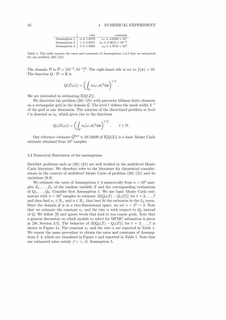
16 4 NUMERICAL EXPERIMENT
rate constantAssumption 1 α ≈ 1.0579 κ1 ≈ 4.0528× 101
Assumption 2 γ ≈ 1.0551 κ3 ≈ 2.3615× 10⁻⁶
Assumption 4 β ≈ 1.9365 κ2 ≈ 1.3744× 10³
Table 1: The table reports the rates and constants of Assumptions 1,2,4 that we estimatedfor our problem (20)–(21).
The domain D is D = [10−4, 10−1]9. The right-hand side is set to f(x) = 10.The function Q : D → R is
Q(Z(ω)) =
(∫Gu(ω,x)2dx
)1/2
.
We are interested in estimating E[Q(Z)].We discretize the problem (20)–(21) with piecewise bilinear finite elements
on a rectangular grid in the domain G. The level ` defines the mesh width 2−`
of the grid in one dimension. The solution of the discretized problem at level` is denoted as u`, which gives rise to the functions
Q`(Z(ω)) =
(∫Gu`(ω,x)2dx
)1/2
, ` ∈ N .
Our reference estimate QRef ≈ 10.54829 of E[Q(Z)] is a basic Monte Carloestimate obtained from 104 samples
4.2 Numerical illustration of the assumptions
Dirichlet problems such as (20)–(21) are well studied in the multilevel MonteCarlo literature. We therefore refer to the literature for theoretical consider-ations in the context of multilevel Monte Carlo of problem (20)–(21) and itsvariations [9,8].
We estimate the rates of Assumptions 1–4 numerically from n = 104 sam-ples Z1, . . . , Zn of the random variable Z and the corresponding evaluationsof Q3, . . . , Q8. Consider first Assumption 1. We use basic Monte Carlo esti-mators with n = 104 samples to estimate |E[Q8(Z)−Q`(Z)]| for ` = 3, . . . , 7and then find κ1 ∈ R+ and α ∈ R+ that best fit the estimates in the L2 norm.Since the domain G is in a two-dimensional space, we set s = 22 = 4. Notethat we estimate the constant κ1 and the rate α with respect to Q8 insteadof Q. We follow [9] and ignore levels that lead to too coarse grids. Note thata general discussion on which models to select for MFMC estimation is givenin [38, Section 3.5]. The behavior of |E[Q8(Z) − Q`(Z)]| for ` = 3, . . . , 7 isshown in Figure 1a. The constant κ1 and the rate α are reported in Table 1.We repeat the same procedure to obtain the rates and constants of Assump-tions 2–4, which are visualized in Figure 1 and reported in Table 1. Note thatour estimated rates satisfy β > γ, cf. Assumption 5.

4.2 NUMERICAL ILLUSTRATION OF THE ASSUMPTIONS 17
1e-03
1e-02
1e-01
1e+00
4 5 6 7
expectedvalue
level `
E[|Q8(Z)−Q`(Z)|]rate α ≈ 1.0579
1e-04
1e-03
1e-02
1e-01
1e+00
4 5 6 7
costs[s]
level `
costs w`rate γ ≈ 1.0551
(a) expected absolute error (b) runtime
1e-06
1e-04
1e-02
1e+00
1e+02
4 5 6 7
variance
level `
Var[Q`(Z)−Q`−1(Z)]rate β ≈ 1.9365
ρ2` − ρ2`−1rate ≈ 1.9883
1e+00
1e+01
1e+02
4 5 6 7
variance
level `
Var[Q`(Z)]
rate 0.0078
(c) decay of variance (d) variance
Fig. 1: The plot in (a) shows that the rate of the decay of the expected absolute error isα ≈ 1, see Assumption 1. The plot in (b) reports the rate γ ≈ 1 of the increase of the runtimeof the evaluations Q` for ` = 3, . . . , 7, see Assumption 2. The plots in (c) and (d) reportthe behavior of the variance with respect to Assumption 4 and Assumption 3, respectively.Note that β > γ as required by Assumption 5.
costs [s] variances correlation coefficientslevel ` = 3 2.94× 10⁻⁴ 9.41 9.990894578× 10⁻¹
level ` = 4 8.77× 10⁻⁴ 9.40 9.999374083× 10⁻¹
level ` = 5 3.18× 10⁻³ 9.34 9.999961196× 10⁻¹
level ` = 6 1.54× 10⁻² 9.10 9.999997721× 10⁻¹
level ` = 7 6.78× 10⁻² 8.27 9.999999908× 10⁻¹
Table 2: The table reports the costs w3, . . . , w7 of functions Q3, . . . , Q7, and the sampleestimates of the variances σ2
3 , . . . , σ27 and the correlation coefficients ρ8,3, . . . , ρ8,7 of the
random variables Q3(Z), . . . , Q7(Z) estimated from 104 samples.
We measure the costs of evaluating the functions Q3, . . . , Q7 by averag-ing the runtime over 104 runs. We use Matlab for the implementation andMatlab’s backslash operator to solve systems of linear equations. The timemeasurements were performed on nodes with Xeon E5-1620 CPUs and 32GBRAM. The variances σ2
3 , . . . , σ27 and the correlation coefficients ρ8,3, . . . , ρ8,7
are obtained from 104 samples, see [38]. The costs w3, . . . , w7, the variancesσ23 , . . . , σ
27 , and the correlation coefficients ρ8,3, . . . , ρ8,7 are reported in Table 2.

18 4 NUMERICAL EXPERIMENT
0 = 10 0
0 = 10 -1
0 = 10 -2
0 = 10 -3
0 = 10 -4
0 = 10 -5
10 -2
10 0
10 2
shar
eof
sam
ples[%
]
100%
88.23%
11.76%
87.55%
11.05%
1.39%
87.44%
10.99%
1.38%
0.17%
87.44%
10.99%
1.38%
0.17%
87.42%
10.99%
1.38%
0.17%
0.02%
level ` = 7level ` = 6level ` = 5level ` = 4level ` = 3
(a) multilevel Monte Carlo
0 = 10 0
0 = 10 -1
0 = 10 -2
0 = 10 -3
0 = 10 -4
0 = 10 -5
10 -2
10 0
10 2
shar
eof
sam
ples[%
]
100%
97.76%
2.23%
97.51%
2.23%
0.25%
97.36%
2.29%
0.30%
0.02%
97.36%
2.29%
0.30%
0.02%
97.32%
2.31%
0.31%
0.03%
level ` = 7level ` = 6level ` = 5level ` = 4level ` = 3
(b) MFMC
Fig. 2: The plots report the share of the number of samples of each level in the total numberof samples. MFMC evaluates the coarsest model more often than multilevel Monte Carlo inthis example.
4.3 Numerical illustration of main theorem
For ε ∈ 100, 10−1, . . . , 10−5, we derive multilevel Monte Carlo and MFMCestimates of E[Q(Z)] following Section 2.3 and Section 2.4, respectively. Thenumber of samples for the multilevel Monte Carlo estimators are derived usingthe rates in Table 1. The number of samples and the coefficients for the MFMCestimators are obtained using the costs, variances, and correlation coefficientsreported in Table 2. Figure 2 compares the number of samples obtained withmultilevel Monte Carlo and MFMC. The absolute numbers of samples arereported in Table 3 for multilevel Monte Carlo and in Table 4 for MFMC. Bothmethods lead to similar numbers of samples. MFMC assigns more samples tolevel ` = 3 than multilevel Monte Carlo. A detailed comparison is shown inFigure 3 for ε = 10−5, which illustrates that multilevel Monte Carlo distributesthe number of samples logarithmically among the levels depending on therates β and γ, see Section 2.4. MFMC directly uses the costs, variances, andcorrelation coefficients and derives a more fine-grained distribution among the

4.4 MFMC AND COARSE-GRID (WEAKLY-CORRELATED) MODELS19
MLM
C
MFM
C
10 -2
10 0
10 2sh
are
ofsa
mples[%
] 87.42%
10.99%
1.38%
0.17%
0.02%
97.32%
2.31%
0.31%
0.03%
level ` = 7level ` = 6level ` = 5level ` = 4level ` = 3
Fig. 3: The bar plot shows a detailed comparison of the share of the samples determinedby multilevel Monte Carlo (MLMC) and MFMC for ε = 10−5. Multilevel Monte Carlodistributes the number of samples logarithmically among the levels, whereas MFMC deter-mines a fine-grained distribution of the number of samples. Thus, the bars have the samesize on a logarithmic scale for multilevel Monte Carlo but different sizes for MFMC. Notethat the percent of the share of the total number of samples for each bar is shown in theplot.
levels than multilevel Monte Carlo. We refer to [38] for further investigationson the number of samples in the context of MFMC.
We repeat the multilevel Monte Carlo and the MFMC estimation 100 timesand report in Figure 4 the estimated MSE
e(Q) =1
100
100∑i=1
(Qi − QRef
)2, (22)
where Qi is either a multilevel Monte Carlo estimator or an MFMC estimator,and where QRef is the reference estimate, see Section 4.1. Figure 4 additionallyshows error bars with length
1
99
100∑i=1
(e(Q)−
(Qi − QRef
)2)2
, (23)
which is an estimate of the variance of the error e(Q) if e(Q) is considered as arandom variable. The estimated MSE for the multilevel Monte Carlo and theMFMC estimators are reported in Figure 4. Both estimators lead to similarestimated MSEs, which is in agreement with Theorem 1. The runtime of themultilevel Monte Carlo and the MFMC estimator is reported in Table 3 andTable 4, respectively.
4.4 MFMC and coarse-grid (weakly-correlated) models
The random variables Q3(Z), . . . , Q7(Z) corresponding to levels ` = 3, . . . , 7are highly correlated to the random variable Q8(Z), see Table 2. We now

20 4 NUMERICAL EXPERIMENT
1e-05
1e-04
1e-03
1e-02
1e-01
1e+00
1e+01
1e-02 1e-01 1e+00 1e+01 1e+02
estimated
MSE
runtime [s]
Multilevel Monte Carlo
MFMC
(a) estimated MSE w.r.t. runtime in seconds
1e-05
1e-04
1e-03
1e-02
1e-01
1e+00
1e+01
1e-051e-041e-031e-021e-011e+00
estimated
MSE
tolerance ε
Multilevel Monte Carlo
MFMC
(b) estimated MSE w.r.t. tolerance ε
Fig. 4: The results are in agreement with Theorem 1, which states that the costs of theMFMC estimator with MSE e(QMF
L,mMF ) . ε are bounded by c(QMFL,mMF ) . ε−1 under
Assumptions 1–7. The behavior of the MFMC estimator is similar to the behavior of themultilevel Monte Carlo estimator.
Table 3: The table reports the number of samples used in the multilevel Monte Carlo esti-mator and the runtime in seconds. The runtime is averaged over 100 runs.
ε ` = 3 ` = 4 ` = 5 ` = 6 ` = 7 total time[s]100 1.20× 101 0 0 0 0 1.20× 101 0.00310−1 1.20× 10² 1.60× 101 0 0 0 1.36× 10² 0.05410−2 1.19× 10³ 1.51× 10² 1.90× 101 0 0 1.36× 10³ 0.60610−3 1.19× 10⁴ 1.50× 10³ 1.89× 10² 2.40× 101 0 1.36× 10⁴ 6.49910−4 1.19× 10⁵ 1.50× 10⁴ 1.89× 10³ 2.38× 10² 0 1.36× 10⁵ 64.95510−5 1.19× 10⁶ 1.50× 10⁵ 1.88× 10⁴ 2.37× 10³ 2.99× 10² 1.36× 10⁶ 674.360

21
Table 4: The tables reports the number of samples used in the MFMC estimator. While thetotal number of samples is higher than in multilevel Monte Carlo (see Table 3), the multi-level Monte Carlo method requires more samples than MFMC at higher levels (i.e., moreexpensive evaluations) and thus the runtimes are about the same for each ε ∈ 1, . . . , 10−5.
ε ` = 3 ` = 4 ` = 5 ` = 6 ` = 7 total time[s]100 1.20× 101 0 0 0 0 1.20× 101 0.00310−1 1.75× 10² 4.00× 100 0 0 0 1.79× 10² 0.05110−2 1.88× 10³ 4.30× 101 5.00× 100 0 0 1.92× 10³ 0.55410−3 1.97× 10⁴ 4.65× 10² 6.20× 101 6.00× 100 0 2.02× 10⁴ 6.50510−4 1.96× 10⁵ 4.64× 10³ 6.18× 10² 5.80× 101 0 2.02× 10⁵ 64.96610−5 2.01× 10⁶ 4.80× 10⁴ 6.60× 10³ 7.24× 10² 7.20× 101 2.07× 10⁶ 674.380
costs [s] variances correlation coefficientslevel ` = 1 1.12× 10⁻⁴ 3.23 7.761297293× 10⁻¹
level ` = 2 1.67× 10⁻⁴ 6.09 9.884862151× 10⁻¹
level ` = 3 2.94× 10⁻⁴ 9.41 9.990894578× 10⁻¹
level ` = 4 8.77× 10⁻⁴ 9.40 9.999374083× 10⁻¹
level ` = 5 3.18× 10⁻³ 9.34 9.999961196× 10⁻¹
Table 5: The table reports the costs w1, . . . , w5 of functions Q1, . . . , Q5, and the sample esti-mates of the variances σ2
1 , . . . , σ25 and the correlation coefficients ρ8,1, . . . , ρ8,5 of the random
variables Q1(Z), . . . , Q5(Z) estimated from 104 samples. Note that the costs, variances, andcorrelation coefficients for levels ` = 3, . . . , 7 are reported in Table 2.
consider MFMC with Q1(Z), Q2(Z), . . . , Q5(Z), where we include levels ` =1 and ` = 2. The estimated correlation coefficients, costs, and variancesare reported in Table 5. The random variable Q1(Z) corresponding to level` = 1 is significantly weaker correlated to Q8(Z) than the random vari-ables Q2(Z), . . . , Q5(Z). As in Section 4.2, we measure the rates of Assump-tions 1,2,4, and obtain α ≈ 0.9255, β ≈ 1.6202 and γ ≈ 0.7160. These ratesare similar as the rates reported in Table 1. Note that β > γ.
We derive multilevel Monte Carlo and MFMC estimates of E[Q(Z)] forε ∈ 101, 100, 10−1, 10−2 and report the estimated MSE (22) in Figure 5. Theerror bars show the variance (23). The results illustrate that MFMC achievesan estimated MSE that is in agreement with Theorem 1 also in this case wherethe random variable Q1(Z) corresponding to the coarsest discretization is onlyweakly correlated to Q8(Z). Multilevel Monte Carlo and MFMC show a similarbehavior. We refer to [38, Section 3.4, Section 4.3], where the performance ofMFMC with weakly-correlated models is further investigated analytically andnumerically.
5 Conclusions
The MFMC method provides a general framework for combining multipleapproximations into an estimator of statistics of a random variable that isexpensive (or impossible) to sample. We discussed MFMC in the special casewhere sampling the random variable requires solving a PDE, and where we cansample only approximations that correspond to a hierarchy of discretizations

22 References
1e-03
1e-02
1e-01
1e+00
1e+01
1e-02 1e-01 1e+00
estimated
MSE
runtime [s]
Multilevel Monte CarloMFMC
1e-03
1e-02
1e-01
1e+00
1e+01
1e-021e-011e+001e+01
estimated
MSE
tolerance ε
Multilevel Monte CarloMFMC
(a) estimated MSE w.r.t. runtime in seconds (b) estimated MSE w.r.t. tolerance ε
Fig. 5: The plots report the estimated MSE of multilevel Monte Carlo and the MFMCestimators that combine Q1(Z), . . . , Q5(Z) corresponding to levels ` = 1, . . . , 5. The randomvariables Q1(Z) and Q2(Z) are only weakly correlated to Q8(Z). The MFMC estimatorshows a similar behavior as the multilevel Monte Carlo estimator.
of the PDE. In this setting, and under standard assumptions on the discretiza-tions of the PDE, the MFMC estimator is efficient, which means that the costsof the MFMC estimator with MSE below a threshold are bounded linearly inthe threshold. Our numerical results illustrated the theory.
Acknowledgment
The first and the third author were supported in part by the AFOSR MURIon multi-information sources of multi-physics systems under Award NumberFA9550-15-1-0038, program manager Jean-Luc Cambier, and by the UnitedStates Department of Energy Applied Mathematics Program, Awards DE-FG02-08ER2585 and DE-SC0009297, as part of the DiaMonD MultifacetedMathematics Integrated Capability Center. The second author was supportedby the US Department of Energy Office of Science grant DE-SC0009324 andthe Air Force Office of Scientific Grant FA9550-15-1-0001. Some of the numer-ical examples were computed on the computer cluster of the Munich Centreof Advanced Computing.
References
1. I. Babuska, F. Nobile, and R. Tempone. A stochastic collocation method for ellipticpartial differential equations with random input data. SIAM Journal on NumericalAnalysis, 45(3):1005–1034, 2007.
2. A. Barth, C. Schwab, and N. Zollinger. Multi-level Monte Carlo Finite Element methodfor elliptic PDEs with stochastic coefficients. Numerische Mathematik, 119(1):123–161,Sept. 2011.
3. P. Benner, S. Gugercin, and K. Willcox. A survey of projection-based model reductionmethods for parametric dynamical systems. SIAM Review, 57(4):483–531, 2015.
4. C. Bierig and A. Chernov. Convergence analysis of multilevel Monte Carlo varianceestimators and application for random obstacle problems. Numerische Mathematik,130(4):579–613, 2015.
References 23
5. C. Bierig and A. Chernov. Approximation of probability density functions by the mul-tilevel Monte Carlo maximum entropy method. Journal of Computational Physics,314:661 – 681, 2016.
6. C. Bierig and A. Chernov. Estimation of arbitrary order central statistical momentsby the multilevel Monte Carlo method. Stochastics and Partial Differential EquationsAnalysis and Computations, 4(1):3–40, 2016.
7. H.-J. Bungartz and M. Griebel. Sparse grids. Acta Numerica, 13:1–123, 2004.8. J. Charrier, R. Scheichl, and A. L. Teckentrup. Finite element error analysis of elliptic
PDEs with random coefficients and its application to multilevel Monte Carlo methods.SIAM Journal on Numerical Analysis, 51(1):322–352, 2013.
9. K. A. Cliffe, M. Giles, R. Scheichl, and A. L. Teckentrup. Multilevel Monte Carlomethods and applications to elliptic PDEs with random coefficients. Computing andVisualization in Science, 14(1):3–15, 2011.
10. N. Collier, A.-L. Haji-Ali, F. Nobile, E. von Schwerin, and R. Tempone. A continuationmultilevel Monte Carlo algorithm. BIT Numerical Mathematics, 55(2):399–432, 2015.
11. C. Cortes and V. Vapnik. Support-vector networks. Machine Learning, 20(3):273–297,1995.
12. A. I. J. Forrester and A. J. Keane. Recent advances in surrogate-based optimization.Progress in Aerospace Sciences, 45(1–3):50–79, Jan. 2009.
13. K. A. Forrester A., Sobester A. Engineering design via surrogate modelling: a practicalguide. Wiley, 2008.
14. F. Franzelin, P. Diehl, and D. Pfluger. Non-intrusive uncertainty quantification withsparse grids for multivariate peridynamic simulations. In M. Griebel and A. M.Schweitzer, editors, Meshfree Methods for Partial Differential Equations VII, pages115–143, Cham, 2015. Springer International Publishing.
15. F. Franzelin and D. Pfluger. From data to uncertainty: An efficient integrated data-driven sparse grid approach to propagate uncertainty. In J. Garcke and D. Pfluger,editors, Sparse Grids and Applications - Stuttgart 2014, pages 29–49, Cham, 2016.Springer International Publishing.
16. T. Gerstner and M. Griebel. Numerical integration using sparse grids. NumericalAlgorithms, 18(3):209–232, 1998.
17. T. Gerstner and M. Griebel. Dimension–adaptive tensor–product quadrature. Comput-ing, 71(1):65–87, 2003.
18. M. Giles. Multi-level Monte Carlo path simulation. Operations Research, 56(3):607–617,2008.
19. M. Griebel, H. Harbrecht, and M. Peters. Multilevel quadrature for elliptic paramet-ric partial differential equations on non-nested meshes. Stochastic Partial DifferentialEquations: Analysis and Computations, 2015. submitted.
20. S. Gugercin, A. Antoulas, and C. Beattie. H2 Model Reduction for Large-Scale LinearDynamical Systems. SIAM Journal on Matrix Analysis and Applications, 30(2):609–638, Jan. 2008.
21. M. D. Gunzburger, C. G. Webster, and G. Zhang. Stochastic finite element methodsfor partial differential equations with random input data. Acta Numerica, 23:521–650,5 2014.
22. A.-L. Haji-Ali, F. Nobile, and R. Tempone. Multi-index Monte Carlo: when sparsitymeets sampling. Numerische Mathematik, 132(4):767–806, June 2015.
23. J. M. Hammersley and D. C. Handscomb. Monte Carlo Methods. Methuen London,1964.
24. H. Harbrecht, M. Peters, and M. Siebenmorgen. On multilevel quadrature for ellipticstochastic partial differential equations. In J. Garcke and M. Griebel, editors, SparseGrids and Applications, pages 161–179, Berlin, Heidelberg, 2013. Springer Berlin Hei-delberg.
25. H. Harbrecht, M. Peters, and M. Siebenmorgen. Multilevel accelerated quadraturefor PDEs with log-normally distributed diffusion coefficient. SIAM/ASA Journal onUncertainty Quantification, 4(1):520–551, 2016.
26. S. Heinrich. Multilevel Monte Carlo Methods. In S. Margenov, J. Wasniewski, andP. Yalamov, editors, Large-Scale Scientific Computing, number 2179 in Lecture Notesin Computer Science, pages 58–67. Springer, 2001.

24 References
27. J. Li and D. Xiu. Evaluation of failure probability via surrogate models. Journal ofComputational Physics, 229(23):8966–8980, 2010.
28. J. S. Liu. Monte Carlo strategies in scientific computing. Springer, 2008.29. A. J. Majda and B. Gershgorin. Quantifying uncertainty in climate change science
through empirical information theory. Proceedings of the National Academy of Sciencesof the United States of America, 107(34):14958–14963, Aug. 2010.
30. B. L. Nelson. On control variate estimators. Computers & Operations Research,14(3):219–225, 1987.
31. L. Ng and K. Willcox. Multifidelity approaches for optimization under uncertainty.International Journal for Numerical Methods in Engineering, 100(10):746–772, 2014.
32. L. Ng and K. Willcox. Monte-Carlo information-reuse approach to aircraft conceptualdesign optimization under uncertainty. Journal of Aircraft, pages 1–12, 2015.
33. F. Nobile, R. Tempone, and C. G. Webster. A sparse grid stochastic collocation methodfor partial differential equations with random input data. SIAM Journal on NumericalAnalysis, 46(5):2309–2345, 2008.
34. S. Pauli and P. Arbenz. Determining optimal multilevel Monte Carlo parameters withapplication to fault tolerance. Computers & Mathematics with Applications, 70(11):2638– 2651, 2015.
35. S. Pauli, P. Arbenz, and C. Schwab. Intrinsic fault tolerance of multilevel Monte Carlomethods. Journal of Parallel and Distributed Computing, 84:24 – 36, 2015.
36. B. Peherstorfer, T. Cui, Y. Marzouk, and K. Willcox. Multifidelity importance sampling.Computer Methods in Applied Mechanics and Engineering, 300:490 – 509, 2016.
37. B. Peherstorfer and K. Willcox. Online adaptive model reduction for nonlinear systemsvia low-rank updates. SIAM Journal on Scientific Computing, 37(4):A2123–A2150,2015.
38. B. Peherstorfer, K. Willcox, and M. Gunzburger. Optimal model management for multi-fidelity Monte Carlo estimation. SIAM Journal on Scientific Computing, 38(5):A3163–A3194, 2016.
39. C. Robert and G. Casella. Monte Carlo Statistical Methods. Springer, 2004.40. G. Rozza, D. Huynh, and A. Patera. Reduced basis approximation and a posteriori
error estimation for affinely parametrized elliptic coercive partial differential equations.Archives of Computational Methods in Engineering, 15(3):1–47, 2007.
41. L. Sirovich. Turbulence and the dynamics of coherent structures. Quarterly of AppliedMathematics, 45:561–571, 1987.
42. A. L. Teckentrup, R. Scheichl, M. Giles, and E. Ullmann. Further analysis of mul-tilevel Monte Carlo methods for elliptic PDEs with random coefficients. NumerischeMathematik, 125(3):569–600, 2013.
43. E. Ullmann, H. C. Elman, and O. G. Ernst. Efficient iterative solvers for stochasticGalerkin discretizations of log-transformed random diffusion problems. SIAM Journalon Scientific Computing, 34(2):A659–A682, 2012.
44. E. Ullmann and I. Papaioannou. Multilevel estimation of rare events. SIAM/ASAJournal on Uncertainty Quantification, 3(1):922–953, 2015.
45. E. Ullmann and C. E. Powell. Solving log-transformed random diffusion problems bystochastic Galerkin mixed finite element methods. SIAM/ASA Journal on UncertaintyQuantification, 3(1):509–534, 2015.
46. V. Vapnik. Statistical Learning Theory. Wiley, 1998.47. D. Xiu. Fast numerical methods for stochastic computations: A review. Communications
in computational physics, 5:242–272, 2009.