CONVENTIONAL MAGNETS – I

Neil Marks.Daresbury Laboratory, Warrington, UK.

1. INTRODUCTION

This first paper is restricted to direct current situations, in which voltages generated by therate of change of flux and the resulting eddy-current effects are negligible. This situation thereforeincludes slowly varying magnets used to ramp the energy of beams in storage rings, together withthe normal effects of energising and de-energising magnets in fixed energy machines.

Formally, the term 'field' refers to the magneto-motive force in a magnetic circuit, expressedin Amps/metre and for which the conventional symbol is H. In a medium or free space thisgenerates a magnetic flux (units Webers, symbol Φ ). The flux per unit cross section is referredto as either the 'flux density' or the 'induction'; this has units of Tesla (T) and symbol B. Studentsnew to the topic may well be confused by the almost universal habit, in conversations involvingaccelerator and magnet practitioners, of referring to 'flux density' also as 'field'. This can bejustified by the identical nature of the distributions of the two quantities in areas of constantpermeability and, particularly, in free space. This, of course, is not the case for the units of the twoquantities. Hence, when distributions only are being referred to, this paper will also use the termfield for both quantities. Further difficulties may arise due to the use of the old unit Gauss (andKilo-Gauss) as the unit of flux density (1T = 104 G) in some computer codes.

2 MAGNETO-STATIC THEORY

2.1 Allowed Flux Density Distributions in Two Dimensions.

A summary of the conventional text-book theory for the solution of the magneto-staticequations in two dimension is presented in Box 1. This commences with the two Maxwellequations that are relevant to magneto-statics:

AbstractThe design and construction of conventional, steel-cored, direct-currentmagnets are discussed. Laplace's equation and the associated cylindricalharmonic solutions in two dimensions are established. The equations areused to define the ideal pole shapes and required excitation for dipole,quadrupole and sextupole magnets. Standard magnet geometries are thenconsidered and criteria determining the coil design are presented. The useof codes for predicting flux density distributions and the iterative tech-niques used for pole face design are then discussed. This includes adescription of the use of two-dimensional codes to generate suitablemagnet end geometries. Finally, standard constructional techniques forcores and coils are described.

div B=0

curl H =j

The assumption is made, at thisstage, that electric currents are notpresent in the immediate region of theproblem and hence j , the vector cur-rent density, is zero. The fuller signifi-cance of this will appear later; it doesnot imply that currents are absentthroughout all space.

With the curl of the magneticfield equal to zero, it is then valid toexpress the induction as the gradientof a scalar function Φ, known as themagnetic scalar potential. Combiningthis with the divergence equation givesthe well known Laplace's equation.

The problem is then limited totwo dimensions and the solution forthe scalar potential in polar coordi-nates (r, θ) for Laplace's equation isgiven in terms of constants E, F, G, andH, an integer n, and an infinite serieswith constants J

n, K

n, L

n and N

n. The

terms in (ln r) and in r -n in the summa-tion all become infinite as r tends tozero, so in practical situations the co-efficients of these terms are zero. Like-wise, the term in θ is many valued, soF can also be set to zero.

This gives a set of cylindricalharmonic solutions for Φ expressed interms of the integer n and and twoassociated constants J

n and K

n. It will

be

Maxwell's equations for magneto-statics:

∇.B = 0 ;∇×H = j ;

In the absence of currents:j = 0.

Then we can put:B = ∇ Φ

so that:∇2 Φ = 0 (Laplace's equation)

where Φ is the magnetic scalar potential.

Taking the two dimensional case (constant in thez direction) and solving for coordinates (r,θ):

Φ = (E+Fθ)(G+H ln r) ∑n=1

∞ (J

n r n cos nθ +

Kn r n sin nθ +L

n r -n cos nθ + M

n r -n sin nθ )

In practical magnetic applications, this becomes:

Φ= ∑n (J

n r n cos nθ +K

n r n sin nθ),

with n integral and Jn,K

n a function of geometry.

This gives components of flux density:

Br = ∑

n (n J

n r n-1 cos nθ +nK

n r n-1 sin nθ)

Bθ = ∑n (-nJ

n r n-1 sin nθ +nK

n r n-1 cos nθ)

Box 1: Magnetic spherical harmonicsderived from Maxwell's equations.

seen that these are determined from the geometry of the magnet design. By considering the gradof Φ, equations for the components of the flux density (B

r and Bθ) are obtained as functions of

r and θ.

It must be stressed that all possible physical distributions of flux density in two dimensionsare described by these equations. For a particular value of n, there are two degrees of freedomgiven by the magnitudes of the corresponding values of J and K; in general these connect thedistributions in the two planes. Hence, once the values of the two constants are defined, the

distributions in both planes are also defined. Behaviour in the vertical plane is determined by thedistribution in the horizontal plane and vice versa; they are not independent of each other. Thepractical significance of this is that, provided the designer is confident of satisfying certainsymmetry conditions (see later section), it is not necessary to be concerned with the design or themeasurement of magnets in the two transverse dimensions; a one-dimensional examination willusually be sufficient.

The condition relating to the presence of currents can now be defined in terms of the polarcoordinates. The solution for Φ in Box 1 is valid providing currents are absent within the rangeof r and θ under consideration. In practical situations, this means areas containing free space andcurrent-free ferro-magnetic material, up to but excluding the surfaces of current-carryingconductors, can be considered.

2.2 Dipole, Quadrupole and Sextupole Magnets

Each value of the integer n in the magnetostatic equations corresponds to a different fluxdistribution generated by different magnet geometries. The three lowest values, n=1, 2, and 3correspond to dipole, quadrupole and sextupoles flux density distributions respectively; this ismade clearer in Boxes 2, 3 and 4. In each case the solutions in Cartesian coordinates are alsoshown, obtained from the simple transformations:

Bx = B

r cos θ - Bθ sin θ,

By = B

r sin θ + Bθ cos θ.

For the dipole field (Box 2),the lines of equipotential, for theJ=0, K non-zero case, are equis-paced and parallel to the x axis.The gradient gives a constant ver-tical field; if J were zero, the linesof B would be horizontal. Thistherefore is a simple, constantmagnetic distribution combiningvertical and horizontal flux densi-ties, according to the values of Jand K and is the common magneticdistribution used for bending mag-nets in accelerators.

Note that we have not yetaddressed the conditions necessaryto obtain such a distribution.

Cylindrical: Cartesian:

Br = J

1 cos θ + K

1 sin θ; B

x = J

1

Bθ = -J1 sin θ + K

1 cos θ; B

y = K

1

Φ = J1 r cos θ +K

1 r sin θ. Φ = J

1 x +K

1 y

So, J1 = 0, K

1 ≠ 0 gives vertical dipole field:

K1 =0, J

1 ≠ 0 gives horizontal dipole field.

Box 2: Dipole field given by n=1 case.

B

φ = const.

For the n=2 case (Box 3) the quadrupole field is generated by lines of equipotential havinghyperbolic form. For the J=0 case, the asymptotes are the two major axes and the flux distributionsare normal to the axes at the axes; the amplitudes of the horizontal and vertical components varylinearly with the displacements from the origin. With zero induction in both planes at the origin,this distribution provides linear focusing of particles. As explained in the paper on linear optics,a magnet that is focusing in one plane will defocus in the other. This is an important example ofthe point explained above; the distributions in the two planes cannot be made independent of eachother.

The J=0 case dealt with above is described as the normal quadrupole field. For zero valueof the constant K (non-zero J) the situation is rotated by π/4 and the distribution is referred to asa skew quadrupole field.

The equations for sextupole field distribution are given in Box 4. Again, the normalsextupole distribution corresponds to the J=0 case. Note the lines of equipotential with six-foldsymmetry and the square law dependency of the vertical component of flux density withhorizontal position on the x axis. As explained in the papers dealing with particle optics, normalsextupole field is used to control chromaticity - the variation in focusing with particle momentum.

Cylindrical: Cartesian:

Br = 2 J

2 r cos 2θ +2K

2 r sin 2θ; B

x = 2 (J

2 x +K

2 y)

Bθ = -2J2 r sin 2θ +2K

2 r cos 2θ; B

Y = 2 (-J

2 y +K

2 x)

Φ = J2 r 2 cos 2θ +K

2 r 2 sin 2θ; Φ = J

2 (x2 - y2)+2K

2 xy

These are quadrupole distributions, with J2 = 0 giving 'normal'

quadrupole field.

Then K2 = 0 gives 'skew' quadrupole fields (which is the above rotated by

π/4).

Box 3: Quadrupole field given by n=2 case.

B

φ = - C φ = + C

φ = + C φ = - C

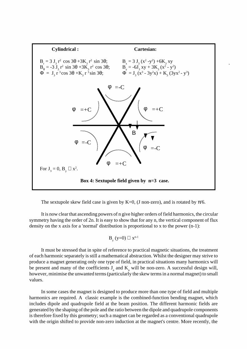
Cylindrical : Cartesian:

Br = 3 J

3 r2 cos 3θ +3K

3 r2 sin 3θ; B

x = 3 J

3 (x2 -y2) +6K

3 xy

Bθ = -3 J3 r2 sin 3θ +3K

3 r2 cos 3θ; B

y = -6J

3 xy + 3K

3 (x2 - y2)

Φ = J3 r 3 cos 3θ +K

3 r 3 sin 3θ; Φ = J

3 (x3 - 3y2x) + K

3 (3yx2 - y3)

For J3 = 0, B

y ∝ x2.

Box 4: Sextupole field given by n=3 case.

φ =+C

=-Cφ

φ =+C

φ =+C

=-Cφ=-Cφ

Β

The sextupole skew field case is given by K=0, (J non-zero), and is rotated by π/6.

It is now clear that ascending powers of n give higher orders of field harmonics, the circularsymmetry having the order of 2n. It is easy to show that for any n, the vertical component of fluxdensity on the x axis for a 'normal' distribution is proportional to x to the power (n-1):

By (y=0) ∝ xn-1

It must be stressed that in spite of reference to practical magnetic situations, the treatmentof each harmonic separately is still a mathematical abstraction. Whilst the designer may strive toproduce a magnet generating only one type of field, in practical situations many harmonics willbe present and many of the coefficients J

n and K

n will be non-zero. A successful design will,

however, minimise the unwanted terms (particularly the skew terms in a normal magnet) to smallvalues.

In some cases the magnet is designed to produce more than one type of field and multipleharmonics are required. A classic example is the combined-function bending magnet, whichincludes dipole and quadrupole field at the beam position. The different harmonic fields aregenerated by the shaping of the pole and the ratio between the dipole and quadrupole componentsis therefore fixed by this geometry; such a magnet can be regarded as a conventional quadrupolewith the origin shifted to provide non-zero induction at the magnet's centre. More recently, the

criticality of space in accel-erator lattices has led to theinvestigation of geometriescapable of generating dipole,quadrupole and sextupolefield in the same magnet, withindependent control of theharmonic amplitudes, and anumber of successful designshave been produced.

2.3 Ideal Pole Shapes

To the basic theoreti-cal concepts of the field har-monics, we shall now add themore practical issue of theferro-magnetic surfaces re-quired to make up the magnetpoles. To many, it is intui-tively obvious that the cor-rect pole shape to generate aparticular harmonic, for theideal case of infinite permea-bility, is a line of constantscalar potential. This is ex-plained more fully in Box 5.This is the standard text bookpresentation for proving thatflux lines are normal to a sur-face of very high permeabil-ity; it then follows from

At the steel boundary, with no currents in the steel:

curl H =0

Apply Stoke's theorem to a closed loop enclosing theboundary:

∫ ∫ (curl H).dS = ∫ H.ds

Hence around the loop: H. ds =0

But for infinite permeability in the steel: H=0;

Therefore outside the steel H=0 parallel to the bound-ary.

Therefore B in the air adjacent to the steel is normal tothe steel surface at all points on the surface.

Therefore from B=grad Φ, the steel surface is an iso-scalar-potential line.

Box 5: Ideal pole shapes are lines of equal magnetic

Steel, µ = ∞

Air

d

ds

sB

For normal (ie not skew) fields:

Dipole:y= ± g/2;

(g is interpole gap).

Quadrupole:xy= ± R2/2;

(R is inscribed radius).

Sextupole:3x2y - y3 = ± R3;

Box 6: Equations of ideal pole shape

the definition:

B = grad Φ

that this is also an equi-potential line.

The resulting ideal pole shapes for(normal) dipole, quadrupole and sextupolemagnets are then given in Box 6. These areobtained from the Cartesian equipotentialequations with the J coefficients set to zero,and geometric terms substituted for K. Forperfect, singular harmonics, infinite polesof the correct form, made from infinitepermeability steel with currents of the cor-rect

Magnet Symmetry Constraint

Dipole φ(θ) = −φ(2π -θ) All Jn =

0;

φ(θ) = φ(π -θ) Kn non-zero only for:

n = 1, 3, 5, etc;

Quadrupole φ(θ) = −φ(π -θ) Kn = 0 for all odd n;

φ(θ) = −φ(2π -θ) All Jn =

0;

φ(θ) = φ(π/2 -θ) Kn non-zero only for:

n = 2, 6, 10, etc;

Sextupole. φ(θ) = −φ(2π/3 -θ) Kn = 0 for all n not

φ(θ) = −φ(4π/3 -θ) multiples of 3;φ(θ) = −φ(2π -θ) All J

n =

0;

φ(θ) = φ(π/3 -θ) Kn non-zero only for:

n = 3, 9, 15, etc.

Box 7: Symmetry constraints in normal dipole, quadrupole andsextupole geometries.

magnitude and polarity located at infinity are sufficient; in practical situations they are happilynot necessary. It is possible to come close to the criterion relating to the steel permeability, forvalues of µ in the many thousands are possible, and the infinite permeability approximation givesgood results in practical situations. Various methods are available to overcome the necessaryfinite sizes of practical poles and certain combinations of conductor close to high-permeabilitysteel produce good distributions up to the surface of the conductors. Before examining such'tricks', we shall first investigate the theoretical consequences of terminating the pole accordingto a practical geometry.

2.4 Symmetry Constraints

The magnet designer will use the ideal pole shapes of Box 6 in the centre regions of the poleprofile, but will terminate the pole with some finite width. In so doing, certain symmetries willbe imposed on the magnet geometry and these in turn will constrain the harmonics that can bepresent in the flux distribution generated by the magnet. The situation is defined in a moremathematical manner in Box 7.

In the case of the normal, vertical field dipole, the designer will place two poles equi-distantfrom the horizontal centre line of the magnet; these will have equal magnitude but oppositepolarity of scalar potential. This first criterion ensures that the values of J

n are zero for all n.

Providing the designer ensures that the pole 'cut-offs' of both the upper and lower pole aresymmetrical about the magnet's vertical centre line, the second symmetry constraint will ensurethat

all Kn values are zero for even n. Thus, with two simple symmetry criteria, the designer has ensured

that the error fields that can be present in the dipole are limited to sextupole, decapole, fourteen-pole, etc.

In the case of the quadrupole, the basic four-fold symmetry about the horizontal and verticalaxes (the first two criteria) render all values of J

n and the values of K

n for all odd n equal to zero.

The third constraint concerns the eight-fold symmetry ie the pole cut-offs being symmetricalabout the π/4 axes. This makes all values of K

n zero, with the exception of the coefficients that

correspond to n=2 (fundamental quadrupole), 6, 10, etc. Thus in a fully symmetric quadrupolemagnet, the lowest-order allowed field error is twelve pole (duodecapole), followed by twentypole, etc.

Box 7 also defines the allowed error harmonics in a sextupole and shows that with the basicsextupole symmetry, eighteen pole is the lowest allowed harmonic error; the next is thirty pole.Higher order field errors are therefore usually not of high priority in the design of a sextupolemagnet.

Given the above limitations on the possible error fields that can be present in a magnet, themagnet designer has additional techniques that can be used to reduce further the errors in thedistribution; these usually take the form of small adjustments to the pole profile close to the cut-off points.

It must be appreciated that the symmetry constraints described in this section apply tomagnet geometries as designed. Construction should closely follow the design but small toleranceerrors will always be present in the magnet when it is finally assembled and these will break thesymmetries described above. Thus, a physical magnet will have non-zero values of all J and Kcoefficients. It is the task of the magnet engineer to predict the distortions resulting frommanufacturing and assembly tolerances; this information then becomes the basis for thespecification covering the magnet manufacture, so ensuring that the completed magnet will meetits design criteria.

Before leaving the topic of magnetic cylindrical harmonics, it is necessary to put thisconcept into the wider context of the interaction of beams with magnetic fields. Particles are notable to carry out a cylindrical harmonic analysis and are therefore not sensitive to the amplitudeor phase of a particular harmonic in a magnet. They see flux densities B and, in resonance typephenomena, the spatial differentials of B, sometimes to high orders. It is a mistake, therefore, toassociate a certain order of differential with one particular harmonic, as all the higher harmonicterms will contribute to the derivative; the magnet designer may well have balanced theamplitudes and polarities of a number of quite high harmonics to meet successfully a stringent fluxdensity criterion within the defined good field region of the magnet.

The two-dimensional cylindrical harmonics are therefore a useful theoretical tool and givea valuable insight into the allowed spatial distributions of magnetic fields. However, whenjudging the viability of a design or the measurements from a completed magnet, always re-assemble the harmonic series and examine the flux density or its derivatives. These are thequantities corresponding to the physical situation in an accelerator magnet.

3 PRACTICAL ASPECTS OFMAGNET DESIGN

3.1 Coil Requirements

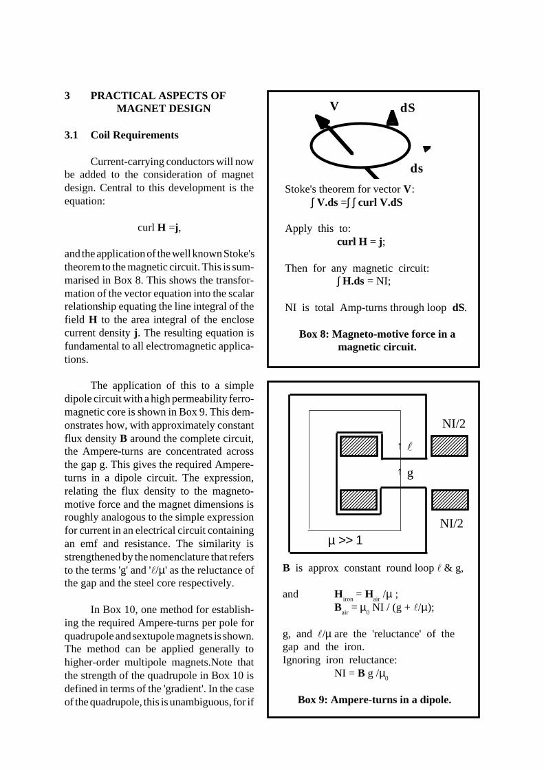
Current-carrying conductors will nowbe added to the consideration of magnetdesign. Central to this development is theequation:

curl H =j ,

and the application of the well known Stoke'stheorem to the magnetic circuit. This is sum-marised in Box 8. This shows the transfor-mation of the vector equation into the scalarrelationship equating the line integral of thefield H to the area integral of the enclosecurrent density j . The resulting equation isfundamental to all electromagnetic applica-tions.

The application of this to a simpledipole circuit with a high permeability ferro-magnetic core is shown in Box 9. This dem-onstrates how, with approximately constantflux density B around the complete circuit,the Ampere-turns are concentrated acrossthe gap g. This gives the required Ampere-turns in a dipole circuit. The expression,relating the flux density to the magneto-motive force and the magnet dimensions isroughly analogous to the simple expressionfor current in an electrical circuit containingan emf and resistance. The similarity isstrengthened by the nomenclature that refersto the terms 'g' and 'l/µ' as the reluctance ofthe gap and the steel core respectively.

In Box 10, one method for establish-ing the required Ampere-turns per pole forquadrupole and sextupole magnets is shown.The method can be applied generally tohigher-order multipole magnets.Note thatthe strength of the quadrupole in Box 10 isdefined in terms of the 'gradient'. In the caseof the quadrupole, this is unambiguous, for if

Stoke's theorem for vector V:∫ V.ds =∫ ∫ curl V.dS

Apply this to:curl H = j ;

Then for any magnetic circuit:∫ H.ds = NI;

NI is total Amp-turns through loop dS.

Box 8: Magneto-motive force in amagnetic circuit.

dS

ds

V

B is approx constant round loop l & g,

and Hiron

= Hair

/µ ;B

air = µ

0 NI / (g + l/µ);

g, and l/µ are the 'reluctance' of thegap and the iron.Ignoring iron reluctance:

NI = B g /µ0

Box 9: Ampere-turns in a dipole.

123456789012123456789012123456789012123456789012123456789012123456789012123456789012

1234567890123123456789012312345678901231234567890123123456789012312345678901231234567890123

123456789012123456789012123456789012123456789012123456789012123456789012123456789012

1234567890123123456789012312345678901231234567890123123456789012312345678901231234567890123

NI/2

NI/2µ >> 1

↑ l

↑ g

the field is expressed as:

By = gx

where g is the quadrupole gradient, then

dBy /dx = g

ie, g is both the field coefficient and themagnitude of the first derivative. For asextupole, the second differential istwice the corresponding coefficient:

By = g

S x2

d2By /dx2 = 2 g

S

In the case of sextupoles and higherorder fields, it is therefore essential tostate whether the coefficient or thederivative is being defined.

3.2 Standard Magnet Geometries

A number of standard dipole magnetgeometries are described in Box 11. Thefirst diagram shows a 'C-core' magnet.The coils are mounted around the upperand lower poles and there is a single asym-metric backleg. In principal, this asymme-try breaks the standard dipole symmetry

Quadruple has pole equation:

xy = R2 /2.On x axes

By = gx,

g is gradient (T/m).

At large x (to give vertical B):

NI = (gx) ( R2 /2x)/µ0

ieNI = g R2 /2 µ

0(per pole)

Similarly, for a sextupole, (field coeffi-cient g

S,), excitation per pole is:

NI = gS R3/3 µ

0

Box 10: Ampere-turns inquadrupole and sextupole.

described in section 2.4 but, providing the core has high permeability, the resulting field errorswill be small. However, a quadrupole term will normally be present, resulting in a gradient of theorder of 0.1% across the pole. As this will depend on the permeability in the core, it will be non-linear and vary with the strength of the magnet.

To ensure good quality dipole field across the required aperture, it is necessary tocompensate for the finite pole width by adding small steps at the outer ends of each of the pole;these are called shims. The designer must optimise the shim geometry to meet the fielddistribution requirements. The maximum flux density across the pole face occurs at thesepositions, and as the shims project above the face, it is essential to ensure that their compensatingeffect is present at all specified levels of magnet operation. Some designers prefer to make thepoles totally flat, resulting in a considerable increase in required pole width to produce the sameextent of good field that would be achieved by using shims. Non-linear effects will still be present,but these will not be as pronounced as in a shimmed pole.

The C-core represents the standard design for the accelerator dipole magnet. It is straight

x B

Box 11: Dipole goemetries, with advantages and disadvantages.

123456789012312345678901231234567890123123456789012312345678901231234567890123

123456789012312345678901231234567890123123456789012312345678901231234567890123

123456789012312345678901231234567890123123456789012312345678901231234567890123

123456789012312345678901231234567890123123456789012312345678901231234567890123

Shim Detail

'C' Core:

Advantages:Easy access;Classic design;

Disadvantages:Pole shims needed;Asymmetric (small);Less rigid;

'H' Type

Advantages:Symmetric;More rigid;

Disadvantages:Also needs shims;Access problems.

'Window Frame'

Advantages:No pole shim;Symmetric;Compact;Rigid;

Disadvantages:Major access problems;Insulation thickness.

123456789012312345678901231234567890123123456789012312345678901231234567890123

123456789012312345678901231234567890123123456789012312345678901231234567890123

123456789012312345678901231234567890123123456789012312345678901231234567890123

123456789012312345678901231234567890123123456789012312345678901231234567890123

123456789012312345678901231234567890123123456789012312345678901231234567890123

1234567890123123456789012312345678901231234567890123123456789012312345678901231234567890123 1234567890123

12345678901231234567890123123456789012312345678901231234567890123

1234567890123123456789012312345678901231234567890123123456789012312345678901231234567890123

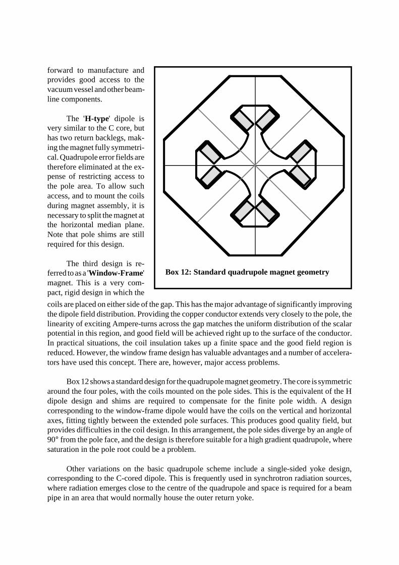
Box 12: Standard quadrupole magnet geometry

forward to manufacture andprovides good access to thevacuum vessel and other beam-line components.

The 'H-type' dipole isvery similar to the C core, buthas two return backlegs, mak-ing the magnet fully symmetri-cal. Quadrupole error fields aretherefore eliminated at the ex-pense of restricting access tothe pole area. To allow suchaccess, and to mount the coilsduring magnet assembly, it isnecessary to split the magnet atthe horizontal median plane.Note that pole shims are stillrequired for this design.

The third design is re-ferred to as a 'Window-Frame'magnet. This is a very com-pact, rigid design in which the

coils are placed on either side of the gap. This has the major advantage of significantly improvingthe dipole field distribution. Providing the copper conductor extends very closely to the pole, thelinearity of exciting Ampere-turns across the gap matches the uniform distribution of the scalarpotential in this region, and good field will be achieved right up to the surface of the conductor.In practical situations, the coil insulation takes up a finite space and the good field region isreduced. However, the window frame design has valuable advantages and a number of accelera-tors have used this concept. There are, however, major access problems.

Box 12 shows a standard design for the quadrupole magnet geometry. The core is symmetricaround the four poles, with the coils mounted on the pole sides. This is the equivalent of the Hdipole design and shims are required to compensate for the finite pole width. A designcorresponding to the window-frame dipole would have the coils on the vertical and horizontalaxes, fitting tightly between the extended pole surfaces. This produces good quality field, butprovides difficulties in the coil design. In this arrangement, the pole sides diverge by an angle of90° from the pole face, and the design is therefore suitable for a high gradient quadrupole, wheresaturation in the pole root could be a problem.

Other variations on the basic quadrupole scheme include a single-sided yoke design,corresponding to the C-cored dipole. This is frequently used in synchrotron radiation sources,where radiation emerges close to the centre of the quadrupole and space is required for a beampipe in an area that would normally house the outer return yoke.

j = NI/AC

where:j is the current density,A

C the area of copper in the coil;

NI is the required Amp-turns.

EC = K (NI)2/A

C

thereforeE

C = (K NI) j

where:E

C is energy loss in coil,

K is a geometrical constatnt.

Therefore, for constant NI, loss varies as j.

Magnet capital costs (coil & yoke materials,plus assembly, testing and transport) vary asthe size of the magnet ie as 1/j.

Total cost of building and running magnet'amortised' over life of machine is:

£ = P + Q/j + R j

P, Q, R and therefore optimum j depend on

design, manufacturer, policy, country, etc.

Box 13: Determination of optimum currentdensity in coils.

3.3 Coil Design

The standard coil design usescopper (or occasionally aluminium)conductor with a rectangular crosssection. Usually, water cooling (lowconductivity de-mineralised water)will be required and in d.c magnetsthis is achieved by having a circularor racetrack-shaped water channelin the centre of the conductor. Thecoil is insulated by glass cloth andencapsulated in epoxy resin.

The main tasks in coil designare determining the optimum totalcross section of conductor in the coiland deciding on the number of indi-vidual turns into which this shouldbe divided.

The factors determining thechoice of current density and hencecopper cross section area are de-scribed in Box 13. Unlike the othercriteria that have been examined inearlier parts of this paper, the primeconsideration determining conduc-tor area is economic. As the area isincreased, the coil, the magnet mate-rial and the manufacturing costs in-crease, whilst the running costs de-crease. The designer must thereforebalance these effects and make apolicy based judgement of the num-ber of years over which the magnetcapital costs will be 'written off'. Theoptimum current density is usuallyin the range of 3 to 5 A/mm2, thoughthis will depend on the relative costof electric power to manufacturingcosts that are applicable. Note thatthe attitude of the funding authorityto a proposed accelerator's capitaland running cost will also have amajor influence on the optimisationof the coil.

£

0 1.0 2.0 3.0 4.0 5.0 6.0

j opt

j (A/mm )2

I ∝ 1/N, Rmagnet

∝ N2 j, Vmagnet

∝ N j, Power ∝ j

Box 14: Variation of magnet parameters with N and j (fixed NI).

Having determined thetotal conductor cross section,the designer must decide onthe number of turns that are tobe used. Box 14 shows howthe current and voltage of acoil vary with the current den-sity j and number of turns percoil, N. This leads to the crite-ria determining the choice ofN, as shown in Box 15.

The choice of a smallnumber of turns leads to highcurrents and bulky terminalsand interconnections, but thecoil packing factor is high. Alarge number of turns leads tovoltage problems. The opti-mum depends on type and sizeof magnet. In a large dipole

Large N (low current) Small N (high current)

* Small, neat terminals. * Large, bulky terminals

* Thin interconnections * Thick, expensive inter- - low cost & flexible. connection.

* More insulation layers * High percentage of in coil, hence larger coil, copper in coil. More increased assembly costs. efficient use of volume.

* High voltage power * High current power supply - safety problems. supply - greater losses.

Box 15: Factors determining choice of N.

magnet, currents in excess of 1,000A are usual, whereas smaller magnets, particularly quad-rupoles and sextupoles would normally operate with currents of the order of a few hundred Amps.In small corrector magnets, much lower currents may be used and if the designer wishes to avoidthe complication of water cooling in such small magnets, solid conductor, rated at a currentdensity of 1A/mm2 or less, may be used; the heat from such a coil can usually be dissipated intothe air by natural convection.

3.4 Steel Yoke Design

The steel yoke provides the essential ferro-magnetic circuit in a conventional magnet,linking the poles and providing the space for the excitation coils. The gross behaviour of themagnet is determined by the the dimensions of the yoke, for an inadequate cross section will resultin excessive flux density, low permeability and hence a significant loss of magneto-motive force(ie Ampere-turns) in the steel. The examination of the properties of steel used in acceleratormagnets will be covered in the second conventional magnet paper, which is concerned with a.c.properties. This paper will therefore be restricted to a few general comments relating to yokedesign and the significance of coercivity in determining residual fields.

The total flux flowing around the yoke is limited by the reluctance of the air gap and hencethe geometry in this region is critical. This is shown in Box 16, indicating that at the gap, in the

g

g

b

Φ ≈ Bgap

(b + 2g) l.

Box 16: Flux at magnet gap.

transverse plane, the flux extends outwardsinto a region of fringe field. A rule of thumbused by magnet designers represents this fringefield as extending by one gap dimension oneither side of the physical edge of the magnet.This then allows the total flux to be expressedin terms of the pole physical breadth plus thefringe field. Sufficient steel must be providedin the top, bottom and backleg regions to limitthe flux density to values that will not allowsaturation in the main body of the yoke. Notehowever that it is usual to have high fluxdensities in the inside corners at the angles ofthe yoke. The flux will be distributed so thatthe reluctance is constant irrespective of thelength of the physical path through the steel

In a continuous ferro-magnetic core, residualfield is determined by the remanence B

R. In a

magnet with a gap having reluctance muchgreater than that of the core, the residual fieldis determined by the coercivity H

C.

With no current in the external coil, the totalintegral of field H around core and gap is zero.

Thus, if Hg is the field in the gap, l and g are

the path lengths in core and gap respectively:

∫l H

C . ds + ∫

gH

g . ds = 0,

B resid

= - µ0 H

C l /g

Box 17: Residual field in gapped magnets.

HC

-

H

B

B R

and this implies that low permeabili-ties will be encountered in the cor-ners. Providing the region of lowpermeability does not extend com-pletely across the yoke, this situationis acceptable.

The effect of the gap fringefield has less significance in the lon-gitudinal direction, for this will addto the strength of the magnet seen bythe circulating beam; a high fringefield will result in the magnet beingrun at a slightly lower induction.Thus, the total longitudinal flux isdetermined by the specified mag-netic length and the fringe field inthis dimension can be ignored whenconsidering both the flux density inthe steel yoke and the inductance inan a.c. magnet.

The yoke will also determinethe residual flux density that can bemeasured in the gap after the magnethas been taken to high field and thenhad the excitation current reduced tozero. In Box 17 it is explained thatthe residual field in a gapped magnetis not determined by the 'remanence'or 'remanent field' (as might be ex-

pected from the names given to these parameters) but by the coercive force (in Amps/m) of thehysteresis loop corresponding to the magnetic excursion experienced by the steel. This is becausethe gap, as previously explained, is the major reluctance in the magnetic circuit and the residualflux density in the gap will be very much less than the remanent field that would be present in anungapped core. The total Ampere-turns around the circuit are zero and hence the positive fieldrequired to drive the residual induction through the gap is equal and opposite to the line integralof (negative) coercive force through the steel.

Typical shims for dipole and quadrupole magnets are shown in Box 18. The dipole shimtakes the form of a trapezoidal extension above the pole face, whilst the quadrupole shim isgenerated from a tangent to the hyperbolic pole, projecting from some point on the pole face andterminating at the extended pole side.

In both cases, the area A of the shim has the primary influence on the edge correction thatis produced. In the dipole case, it is important to limit the height of the shim to prevent saturationin this region at high excitations; this would lead to the field distribution being strongly dependenton the magnet excitation level. On the other hand, if a very low, long shim is used, the nature ofthe field correction would change, with different harmonics being generated. The shim size andshape is therefore a compromise that depends on the field quality that is desired and on the peakinduction in the gap; shim heights and shapes vary widely according to the magnet parameters andthe quality of field that is required.

3.6 Pole Calculations

It is the task of the magnet designer to use iterative techniques to establish a pole face thatproduces a field distribution that meets the field specification: ∆B/B for a dipole, ∆g/g for aquadrupole, etc, over a physical 'good-field region'. The main tool in this investigation is one ormore computer codes that predict the flux density for a defined magnet geometry; these codes will

Dipole Shim:

Quadrupole Shim:

Box 18: Standard pole shims.

A

A

3.5 Pole face design

Whilst this subject is just a particu-lar feature of the yoke design, it is proba-bly the most vital single feature in thedesign of an accelerator magnet, for itwill determine the field distribution seenby the beam and hence control the be-haviour of the accelerator. In the earlypart of this paper, the various types offield were derived from the cylindricalharmonics and the allowed and forbid-den harmonics were established in termsof the magnet's symmetry. It was ex-plained that the remaining error fields,due to there being a non-infinite pole,could then be minimised by the use ofshims at the edges of the pole.

1 08642

Very large pole, no shim

1 08642

Large pole, small shim

Smaller pole, large shim(note change in vertical scale)

Box 19: Effect of shim and polewidth on distribution.

1 08642

be described in the next section. The vari-ables in the optimisation are the width ofthe pole and the size and shape of theshims. For economy sake (particularly inan a.c.magnet where stored energy deter-mines the power supply rating) the de-signer will usually wish to minimise thepole width. Having made an initial esti-mate of a suitable pole width, the magnetdesigner will explore a range of shims in anattempt to establish a good geometry. Ifthis proves to be impossible, the pole widthis increased; if it is easy, economies canpossibly be made by reducing the polewidth. In this work, past experience is veryvaluable, and time and trouble is saved byhaving a rough idea of what will resultfrom a given change.

In an attempt to steer the student whois new to the topic through this ratherintuitive subject, the following brief notesare offered as a guide; they do not repre-sent a definitive procedure for establishinga design:

i) Start with a small shim to explore thesensitivity of the distribution to the shimarea. Use this to obtain a better estimateof the size of shim that you need. In adipole, the shim height will normally bea few percent of the gap, extending overless than five percent of the pole face.

ii) Note that the above numbers are verydependent on the required field quality;very flat dipole fields (of the order of 1part in 104) will need very low shimsand a wide pole, whilst a bigger shim,which produces a significant rise infield at the pole edge before it falls offrapidly, can be used for lower qualityfields. This will give a saving in polewidth. The effects of pole width and shim size are described in Box 19.

iii) When near the optimum, make only small changes to shim height; for an accelerator dipole,with gaps typically between 40 and 60 mm, a 20µm change across the shim makes somedifference when the field is close to optimum. This sensitivity gives a clear indication of the

dimensional tolerances that will be neededduring magnet construction.

iv) In the case of a quadrupole, vary thepoint at which the tangent breaks from thepole; this of course will also vary the posi-tion of the corner of the pole. Make changesof 1 mm or less at the position of the tangentbreak; again, sensitivity to 20µm changes inthe vertical position of the corner will alter the distribution for a typical accelerator quadrupole.

v) For a sextupole, the pole shaping is less critical; the ideal third-order curve would beexpensive to manufacture and is not necessary. Start with a simple rectangular pole and makea linear cut symmetrically placed at each side of the pole. Optimise the depth and angle of thiscut and it will usually be found to be adequate.

vi) When judging the quality of quadrupole and sextupole fields, examine the differentials, notthe fields. When using numerical outputs from the simpler codes, take first or seconddifferences. This is illustrated in Box 20.

vii) In all cases, check the final distribution at different levels of flux density, particularly fullexcitation. If there is a large change in distribution between low and high inductions (and theseare unacceptable), the shims are too high. Start again with a slightly wider pole and a lower,broader shim.

viii) Steel-cored magnets are limited by saturation effects. In dipoles, this appears as an inabilityto achieve high values of flux density without using excessive currents. In the case ofquadrupoles and sextupoles, saturation may also limit the extent of the good field region at fullexcitation. In this case, the only solution is to lengthen the magnet and reduce the gradient.

Dipole: plot (BY

(x) - BY (0))/B

Y (0)

Quad: plot dBY (x)/dx

Sext: plot d2BY(x)/dx2

Box 20: Judgement of field quality.

3.7 Field computation codes

A number of standard codes are available for the pole design process described above. Threewell known packages are compared in Box 21. The first two are simpler, two-dimensional codes,and are ideal for those new to the subject.

MAGNET is a 'classical' two-dimensional magnetostatic code with a finite rectangularmesh, differential analysis and non-linear steel. Separate iterations for the air and steelregions are used to converge on the solution with permeabilities approximating to the physi-cal situation. The first solution (cycle 0) uses infinite permeability in steel; this is then ad-justed on subsequent cycles. Output is B

X and B

Y in air and steel for the complete model, plus

plots of permeability in steel and vector potential in air (to give total fluxes) and (in oneversion) an harmonic analysis. It is quickly and easily learned but suffers from the lack of pre-and post-processing. This means that all input data is numerical and the complete geometryhas to be worked out exactly in Cartesian coordinates before entering into the code. Likewise,the output is in terms of numerical flux densities (in Gauss) and any calculation of gradientsetc must be carried out by hand calculation or by typing into another code. A potentially mis-

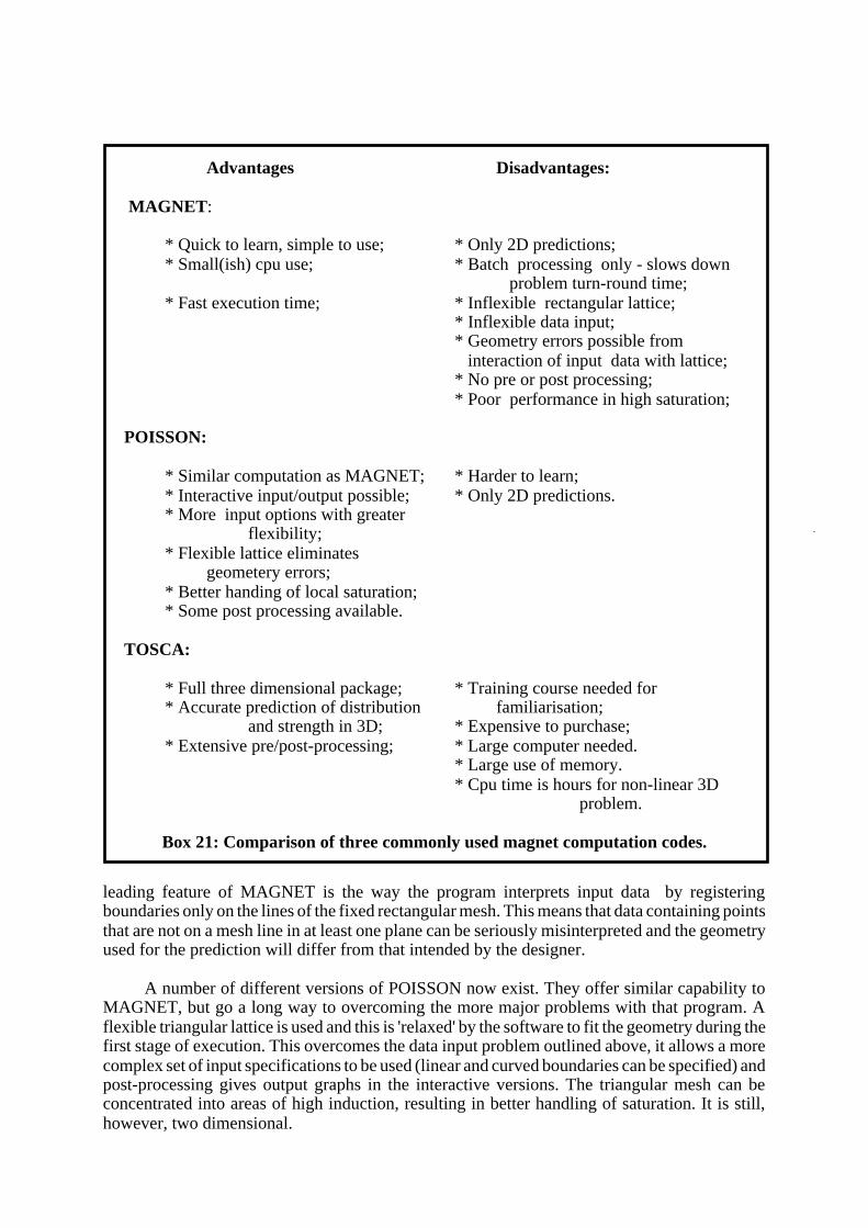
leading feature of MAGNET is the way the program interprets input data by registeringboundaries only on the lines of the fixed rectangular mesh. This means that data containing pointsthat are not on a mesh line in at least one plane can be seriously misinterpreted and the geometryused for the prediction will differ from that intended by the designer.

A number of different versions of POISSON now exist. They offer similar capability toMAGNET, but go a long way to overcoming the more major problems with that program. Aflexible triangular lattice is used and this is 'relaxed' by the software to fit the geometry during thefirst stage of execution. This overcomes the data input problem outlined above, it allows a morecomplex set of input specifications to be used (linear and curved boundaries can be specified) andpost-processing gives output graphs in the interactive versions. The triangular mesh can beconcentrated into areas of high induction, resulting in better handling of saturation. It is still,however, two dimensional.

Advantages Disadvantages:

MAGNET :

* Quick to learn, simple to use; * Only 2D predictions;* Small(ish) cpu use; * Batch processing only - slows down

problem turn-round time;* Fast execution time; * Inflexible rectangular lattice;

* Inflexible data input;* Geometry errors possible from interaction of input data with lattice;* No pre or post processing;* Poor performance in high saturation;

POISSON:

* Similar computation as MAGNET; * Harder to learn;* Interactive input/output possible; * Only 2D predictions.* More input options with greater

flexibility;* Flexible lattice eliminates

geometery errors;* Better handing of local saturation;* Some post processing available.

TOSCA:

* Full three dimensional package; * Training course needed for* Accurate prediction of distribution familiarisation;

and strength in 3D; * Expensive to purchase;* Extensive pre/post-processing; * Large computer needed.

* Large use of memory.* Cpu time is hours for non-linear 3D

problem.

Box 21: Comparison of three commonly used magnet computation codes.

By comparison, TOSCA is a state-of-the-art, three dimensional package that is maintainedand updated by a commercial organisation in U.K. The software suite is available from thiscompany, and training courses are offered to accustom both beginners and more experienceddesigners to the wide range of facilities available in the program.

There are now a large number of field computation packages available for both acceleratorand more general electrical engineering purposes. The decision not to mention a certain packagein this paper does not imply any criticism or rejection of that program. The three chosen fordescription are, however, 'classic' packages that perhaps represent three separate stages in thedevelopment of the computation program.

It should not be believed that the lack of three-dimensional information in the simplerpackages prevents the designer obtaining useful information concerning the magnet in theazimuthal direction. The next two sections will therefore deal with the topic of magnet ends andhow they are addressed numerically.

3.8 Magnet ends

Unless the magnet is playing a relatively unimportant role in the accelerator, the magnetdesigner must pay particular attention to the processes that are occurring at the magnet ends.The situation is summarised in Box 22. A square end (viewed in the longitudinal direction)will collect a large amount of flux from the fringe region and saturation may occur. Such asharp termination also allows no control of the radial field in the fringe region and produces apoor quality distribution. This fringe area will normally contribute appreciably to the inte-grated field seen by the beam, the actual percentage depending on the length of the magnet. Itis quite pointless to carefully design a pole to give a very flat distribution in the centre of themagnet if the end fields totally ruin this high quality. The end distribution, in both the longitu-dinal and transverse planes, must therefore be controlled.

Box 22: Control of longitudinal field distributions in magnet ends.

Square ends:

* display non linear effects (saturation);* give no control of radial distribution in the

fringe region.

Chamfered ends:

* define magnetic length more precisely;* prevent saturation;* control transverse distribution;* prevent flux entering iron normal to

lamination (vital for ac magnets).

Saturation

Dipole:

Quadrupole:

Box 23: Contol of transverse distribu-tion in end regions with non-standard

poles.

This is usually achieved by 'chamfering'or 'rolling off' the magnet end, as shown inBox 22. A number of standard algorithms havebeen described for this, but the exact shape isof no great importance except in very highflux density magnets. The important criteriafor the roll off are:

i) It should prevent appreciable non-linear(saturation) effects at the ends for all levelsof induction.

ii) It should provide the designer with con-trol of transverse distribution throughoutthe region where the fringe flux is contrib-uting appreciably to the magnet strength.

iii) It should not occupy an uneconomicallylarge region.

iv) It should, in a.c. applications, preventappreciable flux entering normal to theplane of the laminations.

practice to profile the magnet pole to attempt to maintain good field quality as the gap increasesand the flux density reduces. Box 23 describes the typical geometries that are used. In the case ofthe dipole, the shim is increased in size as the gap gets larger; for the quadrupole the pole shapeis approximated to the arcs of circles with increasing radii. It should be appreciated that suchtechniques cannot give ideal results, for it must be assumed that the pole width was optimised fora given gap dimension. Hence, no shim will be found that can give a good field distribution withthe same pole width and larger gap. However, the fringe region will only contribute a certainpercentage to the overall field integral and hence the specification can be degraded in this region.In some cases, integrated errors in the end region can be compensated by small adjustments to thecentral distribution; however, to use this technique, the designer must be particularly confidentof the end-field calculations.

3.9 Calculation of end field distributions

Even using two-dimensional codes, numerical estimates of the flux distribution in themagnet ends can be made. The use of an idealised geometry to estimate the longitudinal situationin a dipole is shown in Box 24. The right hand side of the model approximates to the physicalmagnet, with the end roll-off and the coil in the correct physical positions. However, the returnyoke and the coil on the left are non-physical abstractions; they are needed to provide the magneto-motive force and a return path for the flux in the two dimensional model. Thus the flux distributionin the end region will be a good representation of what would be expected on the radial centre planeof the magnet. This model can therefore be used to check the field roll off distribution, the

Looking at these chamfered end regionsin the transverse plane again, it is then the

flux density at the steel surface in the chamfer, and the expected integrated field length of themagnet; this last parameter is, of course, of primary importance as it determines the strength ofthe magnet.

In the case of the quadrupole, the similar calculation is less useful. The same model can beused, taking a section through the 45° line, ie on the inscribed radius, but this will look like a dipoleand predict a non-zero field at the magnet centre. The only useful feature will therefore be anexamination of the flux densities at the steel surface in the end regions by normalising to the valuepredicted for the central region in the transverse calculations. As saturation on the pole is seldomencountered in a quadrupole (if present, it is usually in the root of the pole), this is of little value.

It is not usually necessary to chamfer the ends of sextupoles; a square cut off can be used.

Turning now to the transverse plane in the end region, it is quite practical to makecalculations with the increased pole gap and enlarged shim for each transverse 'slice' through theend. The shim can be worked on to optimise the field distribution as best as possible, and theprediction of transverse distribution used with some confidence. However, the predicted ampli-tude of flux density will be incorrect, for there will be a non-zero field derivative in the planenormal to the two-dimensional model. In principle, the distribution is also invalidated by this term,but experience indicates that this is a small effect. Hence, the designer must normalise theamplitude of the flux density in each 'slice' to that predicted in the longitudinal model. Theresulting normalised distributions can then be numerically integrated (by hand calculation!) andadded to the integrated radial distribution in the body of the magnet. This gives a set of figuresfor the variation of integrated field as a function of radial position - the principal aim of the wholeexercise. Of course, all this can be avoided if a full three-dimensional program is used and thecomplete magnet will be computed in one single execution. However, the above procedure givesa very satisfactory prediction if an advanced code is not available; it also gives the designer a good'feel' for the magnet that is being worked upon.

The diagram shows an idealised geometry in the longitudinal plane of a dipole, asused to estimate end-field distributions. The right hand coil is at the correct physicalposition; the coil and return yoke on the left are idealised to provide excitation and areturn path for the flux in two dimensions.

Box 24: Calculation of longitudinal end effects using two-dimensional codes.

123456781234567812345678123456781234567812345678123456781234567812345678

123456712345671234567123456712345671234567123456712345671234567

-

+

3.10 Magnet manufacture

This is a specialised topic, the details of which are perhaps best left to the variousmanufacturers that make their living by supplying accelerator laboratories. However, a fewcomments should help the designer when preparing for this exercise.

For d.c. accelerator magnets, yokes are usually laminated. This allows the 'shuffling' of steelto randomise the magnetic properties. Laminations also prevent eddy current effects which, evenin d.c. magnets, can cause problems with decay time constants of the order of minutes.Laminations are therefore be regarded as essential in storage rings which are ramped betweeninjection and full energy.

The laminations are 'stamped' using a 'stamping tool'. This must have very high precisionand reproducibility (~20µm). Manufacturers involved in standard electrical engineering produc-tion will regard this figure as stringent but possible. The dimensions of the lamination must bechecked on an optical microscope every five to eight thousand laminations.

Assembly of the laminations is in a fixture; the number of laminations in each stack isdetermined by weight and hydraulic pressure is used to define the length. At one time, the stackedlaminations were glued together, but now it is more usual to weld externally whilst the stack isfirmly held in the fixture. If a.c. magnets are being assembled the welding must not produceshorted turns.

Coils are wound using glass insulation wrapped onto the copper or aluminium conductorbefore receiving an 'outerground' insulation of (thicker) glass cloth. The assembly is then placedin a mould and heated under vacuum to dry and outgas. The mould is subsequently flooded withliquid epoxy resin that has been mixed with the catalyst under vacuum. The vacuum tank is letup to atmosphere, forcing the resin deep into the coil to produce full impregnation. 'Curing' of theresin then occurs at high temperature. Total cleanliness is essential during all stages of thisprocess!

Rigorous testing of coils, including water pressure, water flow, thermal cycling and 'flash'testing at high voltage whilst the body of the coil is immersed in water (terminals only clear) isstrongly recommended. This will pay dividends in reliability of the magnets in the operationalenvironment of the accelerator.

BIBLIOGRAPHY

Many text-books provide a sound theoretical description of fundamental magneto-staticsas described in this paper, but for a clear and easily understood presentation see:

B.I. Bleaney and B. Bleaney, Electricity and Magnetism, (Oxford University Press, 1959)

For a more advanced presentation, see:

W.K.H. Panofsky and M. Phillips, Classical Electricity and Magnetism, (Addison - WesleyPublishing Co., 1956).

Many magnet designs for accelerator applications have been described in detail in the seriesof International Conferences on Magnet Technology. Given below are the dates and venues ofthese conferences; the proceedings of these Conferences provide many examples of d.c, a.c. andpulsed magnet design:

1965 Stanford Ca, USA;1967 Oxford, UK;1970 Hamburg, Germany;1972 Brookhaven N.Y., USA;1975 Rome, Italy;1977 Bratislava, Czechoslovakia1981 Karlsruhe, Germany;1983 Grenoble, France;1985 Zurich, Switzerland;1989 Boston, USA.