convection in ice i with non-newtonian rheology ... · convection in ice i with non-newtonian...

Convection in Ice I With Non-Newtonian

Rheology: Application to the Icy Galilean

Satellites

by

Amy Courtright Barr

B.S., California Institute of Technology, 2000

M.S., University of Colorado, 2002

A thesis submitted to the

Faculty of the Graduate School of the

University of Colorado in partial fulfillment

of the requirements for the degree of

Doctor of Philosophy

Geophysics Graduate Program

Department of Astrophysical and Planetary Sciences

2004

This thesis entitled:Convection in Ice I With Non-Newtonian Rheology: Application to the Icy Galilean

Satelliteswritten by Amy Courtright Barr

has been approved for the Geophysics Graduate ProgramDepartment of Astrophysical and Planetary Sciences

Robert T. Pappalardo

Dr. Robert Grimm

Dr. Bruce Jakosky

Dr. John Wahr

Dr. Shijie Zhong

Date

The final copy of this thesis has been examined by the signatories, and we find thatboth the content and the form meet acceptable presentation standards of scholarly

work in the above mentioned discipline.

iii

Barr, Amy Courtright (Ph. D, Geophysics)

Convection in Ice I With Non-Newtonian Rheology: Application to the Icy Galilean

Satellites

Thesis directed by Prof. Robert T. Pappalardo

Observations from the Galileo spacecraft suggest that the Jovian icy satellites

Europa, Ganymede, and Callisto have liquid water oceans beneath their icy surfaces.

The outer ice I shells of the satellites represent a barrier between their surfaces and their

oceans and serve to decouple fluid motions in their deep interiors from their surfaces.

Understanding heat and mass transport by convection within the outer ice I shells of

the satellites is crucial to understanding their geophysical and astrobiological evolution.

Recent laboratory experiments suggest that deformation in ice I is accommodated

by several different creep mechanisms. Newtonian deformation creep accommodates

strain in warm ice with small grain sizes. However, deformation in ice with larger

grain sizes is controlled by grain-size-sensitive and dislocation creep, which are non-

Newtonian. Previous studies of convection have not considered this complex rheological

behavior.

This thesis revisits basic geophysical questions regarding heat and mass trans-

port in the ice I shells of the satellites using a composite Newtonian/non-Newtonian

rheology for ice I. The composite rheology is implemented in a numerical convection

model developed for Earth’s mantle to study the behavior of an ice I shell during the

onset of convection and in the stagnant lid convection regime. The conditions required

to trigger convection in a conductive ice I shell depend on the grain size of the ice, and

the amplitude and wavelength of temperature perturbation issued to the ice shell.

If convection occurs, the efficiency of heat and mass transport is dependent on

the ice grain size as well. If convection occurs, fluid motions in the ice shells enhance the

iv

nutrient flux delivered to their oceans, and coupled with resurfacing events, may provide

a sustainable biogeochemical cycle. The results of this thesis suggest that evolution of

ice grain size in the satellites and the details of how tidal dissipation perturbs the ice

shell to trigger convection are required to judge whether convection can begin in the

satellites, and controls the efficiency of convection.

Dedication

For Bernice Pedersen Courtright and Alberta Engvall Siegel

vi

Acknowledgements

I would like to thank Bob Pappalardo for sharing his excellence and creativity

with me for four years. The motivation for this thesis stems from a conversation with

Dave Stevenson that occurred when I was a freshman at Caltech. Shijie Zhong and his

post-docs Jeroen Van Hunen and Allen McNamara helped me turn my pile of ideas into

numerically tractable projects. Bill McKinnon, Don Blankenship, Francis Nimmo, and

Bill Moore have repeatedly raised the bar for success by asking tough questions and

listening patiently as I stammered out the answers.

I would not have made it through grad school without an incredible support

network of friends, family, and faculty members. The core of this network is Bernadine

Barr, who served both as mother and seasoned academic advisor. Thanks to the faculty

at CU, especially Fran Bagenal, Jim Green, Bruce Jakosky, Mike Shull, and John Wahr.

Special thanks to Louise Prockter, Geoff Collins, and Jeff Moore, for providing assurance

that there will be life after grad school. Thanks to Erika Barth, David Brain, Shawn

Brooks, G. Wesley Patterson, James Roberts, Andrew Steffl, Dimitri Veras, and Arwen

Vidal. Thanks to my γδβγ-friends Catherine Boone, Kjerstin Easton, Sarah (DEI)

Milkovich, Brian Platt, David (this is all his fault) Tytell, Travis Williams, and Adrianne

and Yifan Yang.

Support for this work was provided by NASA Graduate Student Researchers

Program grant NGT5-50337 and NASA Exobiology grant NCC2-1340.

vii

Contents

Chapter

1 Introduction 1

1.1 Questions Addressed in this Thesis . . . . . . . . . . . . . . . . . . . . . 3

1.2 Geological and Geophysical Setting . . . . . . . . . . . . . . . . . . . . . 3

1.2.1 Basic Properties . . . . . . . . . . . . . . . . . . . . . . . . . . . 3

1.2.2 Surfaces . . . . . . . . . . . . . . . . . . . . . . . . . . . . . . . . 7

1.2.3 Tidal Effects . . . . . . . . . . . . . . . . . . . . . . . . . . . . . 11

1.3 Astrobiological Setting . . . . . . . . . . . . . . . . . . . . . . . . . . . . 15

1.4 Rheology of Ice I . . . . . . . . . . . . . . . . . . . . . . . . . . . . . . . 18

1.5 Convection in Ice I . . . . . . . . . . . . . . . . . . . . . . . . . . . . . . 21

1.5.1 Governing Equations . . . . . . . . . . . . . . . . . . . . . . . . . 22

1.5.2 Non-Dimensional Coordinates . . . . . . . . . . . . . . . . . . . . 26

1.5.3 Viscosity Functions . . . . . . . . . . . . . . . . . . . . . . . . . . 28

1.5.4 Composite Rheology for Ice I . . . . . . . . . . . . . . . . . . . . 29

1.6 The Onset of Convection . . . . . . . . . . . . . . . . . . . . . . . . . . . 33

1.6.1 Linear Stability Analysis . . . . . . . . . . . . . . . . . . . . . . . 33

1.6.2 Non-Newtonian Rheologies . . . . . . . . . . . . . . . . . . . . . 34

1.7 Previous Studies of Convection in the Icy Satellites . . . . . . . . . . . . 36

viii

2 Convective Instability in Ice I with Non-Newtonian Rheology 39

2.1 Abstract . . . . . . . . . . . . . . . . . . . . . . . . . . . . . . . . . . . . 39

2.2 Introduction . . . . . . . . . . . . . . . . . . . . . . . . . . . . . . . . . . 40

2.3 Methods . . . . . . . . . . . . . . . . . . . . . . . . . . . . . . . . . . . . 43

2.3.1 Numerical Implementation of Ice I Rheology . . . . . . . . . . . 43

2.3.2 Numerical Convection Model . . . . . . . . . . . . . . . . . . . . 46

2.3.3 Initial Conditions . . . . . . . . . . . . . . . . . . . . . . . . . . . 48

2.4 Model Results . . . . . . . . . . . . . . . . . . . . . . . . . . . . . . . . . 50

2.4.1 Critical Rayleigh Number . . . . . . . . . . . . . . . . . . . . . . 50

2.4.2 Critical Shell Thickness . . . . . . . . . . . . . . . . . . . . . . . 59

2.4.3 Variation of Melting Temperature . . . . . . . . . . . . . . . . . 59

2.5 Comparison to Existing Studies . . . . . . . . . . . . . . . . . . . . . . . 60

2.6 Implications for the Icy Galilean Satellites . . . . . . . . . . . . . . . . . 65

2.6.1 Conditions for Convection in Callisto and Ganymede . . . . . . . 66

2.6.2 Conditions for Convection in Europa . . . . . . . . . . . . . . . . 71

2.7 Discussion: The Role of Tidal Dissipation . . . . . . . . . . . . . . . . . 73

2.8 Summary . . . . . . . . . . . . . . . . . . . . . . . . . . . . . . . . . . . 76

3 Onset of Convection in Ice I with Composite Newtonian and Non-Newtonian

Rheology 78

3.1 Abstract . . . . . . . . . . . . . . . . . . . . . . . . . . . . . . . . . . . . 78

3.2 Introduction . . . . . . . . . . . . . . . . . . . . . . . . . . . . . . . . . . 79

3.3 Methods . . . . . . . . . . . . . . . . . . . . . . . . . . . . . . . . . . . . 80

3.3.1 Numerical Implementation of Composite Rheology for Ice I . . . 80



3.4 Results . . . . . . . . . . . . . . . . . . . . . . . . . . . . . . . . . . . . . 90

ix

3.5 Implications for the Icy Galilean Satellites . . . . . . . . . . . . . . . . . 100

3.5.1 Conditions for Convection in Europa . . . . . . . . . . . . . . . . 101

3.5.2 Conditions for Convection in Ganymede and Callisto . . . . . . . 103

3.5.3 Role of Tidal Heating . . . . . . . . . . . . . . . . . . . . . . . . 103

3.5.4 Evolution of Grain Size and Orientation . . . . . . . . . . . . . . 106

3.6 Summary and Conclusions . . . . . . . . . . . . . . . . . . . . . . . . . . 107

4 Implications for the Internal Structure of the Major Satellites of the Outer Plan-

ets 110

4.1 Abstract . . . . . . . . . . . . . . . . . . . . . . . . . . . . . . . . . . . . 110

4.2 Introduction . . . . . . . . . . . . . . . . . . . . . . . . . . . . . . . . . . 111

4.3 Methods . . . . . . . . . . . . . . . . . . . . . . . . . . . . . . . . . . . . 111

4.3.1 Numerical Implementation of Ice Rheology . . . . . . . . . . . . 111



4.4 Thermodynamic Stability of Oceans . . . . . . . . . . . . . . . . . . . . 114

4.4.1 Critical Rayleigh Number . . . . . . . . . . . . . . . . . . . . . . 115

4.4.2 Efficiency of Convection . . . . . . . . . . . . . . . . . . . . . . . 115

4.4.3 Ocean Stability Without Tidal Heating . . . . . . . . . . . . . . 119

4.4.4 Presence of Non-Water-Ice Materials . . . . . . . . . . . . . . . . 120

4.4.5 Tidal Dissipation . . . . . . . . . . . . . . . . . . . . . . . . . . . 122

4.5 Summary . . . . . . . . . . . . . . . . . . . . . . . . . . . . . . . . . . . 126

5 Implications for Astrobiology 128

5.1 Abstract . . . . . . . . . . . . . . . . . . . . . . . . . . . . . . . . . . . . 128

5.2 Introduction . . . . . . . . . . . . . . . . . . . . . . . . . . . . . . . . . . 129

5.3 Astrobiological Setting . . . . . . . . . . . . . . . . . . . . . . . . . . . . 130

5.4 Onset of Convection . . . . . . . . . . . . . . . . . . . . . . . . . . . . . 133

x

5.5 Convective Recycling of the Ice Shell . . . . . . . . . . . . . . . . . . . . 138

5.5.1 Geophysical Descriptive Parameters . . . . . . . . . . . . . . . . 139

5.5.2 Astrobiologically Relevant Parameters . . . . . . . . . . . . . . . 140

5.6 Endogenic Resurfacing Events on Europa . . . . . . . . . . . . . . . . . 149

5.6.1 Domes . . . . . . . . . . . . . . . . . . . . . . . . . . . . . . . . . 149

5.6.2 Ridges . . . . . . . . . . . . . . . . . . . . . . . . . . . . . . . . . 152

5.7 Ocean Stability . . . . . . . . . . . . . . . . . . . . . . . . . . . . . . . . 153

5.8 Summary . . . . . . . . . . . . . . . . . . . . . . . . . . . . . . . . . . . 154

6 Conclusions and Future Work 155

6.1 Answers to the Key Questions . . . . . . . . . . . . . . . . . . . . . . . . 155

6.2 Future Work . . . . . . . . . . . . . . . . . . . . . . . . . . . . . . . . . 158

6.2.1 Grain Size Evolution . . . . . . . . . . . . . . . . . . . . . . . . . 158

6.2.2 Tidal Dissipation . . . . . . . . . . . . . . . . . . . . . . . . . . . 159

6.2.3 Premelting in Ice . . . . . . . . . . . . . . . . . . . . . . . . . . . 168

6.3 Synthesis . . . . . . . . . . . . . . . . . . . . . . . . . . . . . . . . . . . 177

Bibliography 179

Appendix

A Thermal, Physical, and Rheological Parameters 186

B Selected Input Parameters 189

xi

Tables

Table

2.1 Variation in critical Rayleigh number with perturbation amplitude . . . 55

2.2 Numerically determined fitting coefficients for Racr . . . . . . . . . . . . 59

2.3 Comparison to analysis of Solomatov (1995) . . . . . . . . . . . . . . . . 62

4.1 Convective heat flux and Nu for 20 km < D < 100 km . . . . . . . . . . 118

4.2 Orbital parameters for Ganymede and Europa . . . . . . . . . . . . . . . 125

6.1 Rheological parameters for T∼ Tm from Goldsby and Kohlstedt (2001) . 169

A.1 Thermal and physical parameters of the satellites . . . . . . . . . . . . . 187

A.2 Rheological parameters, after Goldsby and Kohlstedt (2001) . . . . . . . 188

B.1 Selected input parameters for simulations used to determine the critical

Rayleigh number and wavelength with GBS rheology . . . . . . . . . . . 190


Rayleigh number and wavelength with GBS rheology (continued) . . . . 191


Rayleigh number and wavelength with basal slip rheology . . . . . . . . 192


Rayleigh number and wavelength with basal slip rheology (continued) . 193

xii


Rayleigh number and wavelength with composite rheology . . . . . . . . 194


Rayleigh number and wavelength with composite rheology (continued) . 195

B.7 Weighting values for the composite rheology of ice I . . . . . . . . . . . 196

B.8 Input parameters used in Chapters 4 and 5 . . . . . . . . . . . . . . . . 197

B.9 Input parameters used in Chapters 4 and 5 (continued) . . . . . . . . . 198

xiii

Figures

Figure

1.1 The Galilean satellites of Jupiter . . . . . . . . . . . . . . . . . . . . . . 2

1.2 Phase diagram of water . . . . . . . . . . . . . . . . . . . . . . . . . . . 4

1.3 Interiors of the icy Galliean satellites . . . . . . . . . . . . . . . . . . . . 6

1.4 High resolution image of a double ridge on the surface of Europa . . . . 9

1.5 Pits, spots, and domes on the surface of Europa . . . . . . . . . . . . . . 10

1.6 Chaos terrain on Europa . . . . . . . . . . . . . . . . . . . . . . . . . . . 12

1.7 Grooved terrain on Ganymede . . . . . . . . . . . . . . . . . . . . . . . . 13

1.8 Conceptual diagrams of deformation mechanisms in ice I . . . . . . . . . 20

1.9 Initial temperature perturbation issued to the ice shell . . . . . . . . . . 25

2.1 Onset of convection in ice I with basal slip rheology . . . . . . . . . . . 51

2.2 Evolution of kinetic energy with time . . . . . . . . . . . . . . . . . . . . 52

2.3 Critical Rayleigh number as a function of wavelength . . . . . . . . . . . 54

2.4 Critical Rayleigh number as a function of perturbation amplitude . . . . 56

2.5 Asymptotic and power law regimes . . . . . . . . . . . . . . . . . . . . . 57

2.6 Comparison of Raa to values from Solomatov (1995) . . . . . . . . . . . 64

2.7 Critical ice shell thickness for convection in Callisto . . . . . . . . . . . . 67

2.8 Critical ice shell thickness for convection in Ganymede . . . . . . . . . . 68

2.9 Critical grain size for convection in Callisto . . . . . . . . . . . . . . . . 69

xiv

2.10 Critical grain size for convection in Ganymede . . . . . . . . . . . . . . . 70

2.11 Critical ice shell thickness for convection in Europa . . . . . . . . . . . . 72

2.12 Critical grain size for convection in Europa . . . . . . . . . . . . . . . . 74

3.1 Deformation maps for ice I . . . . . . . . . . . . . . . . . . . . . . . . . 83

3.2 Composite viscosity of ice I as a function of stress . . . . . . . . . . . . 85

3.3 Determination of Racr for convection in ice I with d = 3.0 cm . . . . . . 91

3.4 Temperature and viscosity fields for convection in ice I with composite

rheology and d = 3.0 cm . . . . . . . . . . . . . . . . . . . . . . . . . . . 92

3.5 Example of determination of λcr for ice with composite rheology . . . . 94

3.6 Variation of Racr with perturbation amplitude . . . . . . . . . . . . . . 95

3.7 Variation in Racr,0 as a function of grain size . . . . . . . . . . . . . . . 96

3.8 Activation of non-Newtonian creep mechanisms in ice with 0.1 mm < d <

1.0 cm . . . . . . . . . . . . . . . . . . . . . . . . . . . . . . . . . . . . . 97

3.9 Activation of non-Newtonian creep mechanisms in ice with 1.0 cm < d <

3.0 cm . . . . . . . . . . . . . . . . . . . . . . . . . . . . . . . . . . . . . 99

3.10 Critical shell thickness for convection in Newtonian and non-Newtonian

ice I: Europa . . . . . . . . . . . . . . . . . . . . . . . . . . . . . . . . . 102


ice I: Ganymede . . . . . . . . . . . . . . . . . . . . . . . . . . . . . . . 104


ice I: Callisto . . . . . . . . . . . . . . . . . . . . . . . . . . . . . . . . . 105

4.1 Convective parameter space explored . . . . . . . . . . . . . . . . . . . . 116

4.2 Variation in convective and conductive heat flux with ice shell thickness

and grain size . . . . . . . . . . . . . . . . . . . . . . . . . . . . . . . . . 121

5.1 Geophysical processes relevant to astrobiology in the Galilean satellites . 132

xv

5.2 Critical wavelength for convection in ice I with composite rheology . . . 136

5.3 Critical shell thickness for convection with composite rheology . . . . . . 137

5.4 Convective parameter space explored . . . . . . . . . . . . . . . . . . . . 141

5.5 Convection in an ice shell 85 km thick with composite rheology and d=0.3

mm . . . . . . . . . . . . . . . . . . . . . . . . . . . . . . . . . . . . . . 142

5.6 Convection in an ice shell 85 km thick with composite rheology and d=30

mm . . . . . . . . . . . . . . . . . . . . . . . . . . . . . . . . . . . . . . 143

5.7 Calculation of interior temperature, stagnant lid thickness, and mass flux 144

5.8 Variation in stagnant lid thickness with grain size . . . . . . . . . . . . . 145

5.9 Mass flux delivered to the stagnant lid . . . . . . . . . . . . . . . . . . . 147

5.10 Recycling time scale for the convecting sublayer of the ice shell . . . . . 148

5.11 Dynamic topography due to convection on Europa . . . . . . . . . . . . 151

6.1 Deformation maps for ice I with high temperature creep enhancement

(d =0.1 mm and d =1 mm) . . . . . . . . . . . . . . . . . . . . . . . . . 171

6.2 Deformation maps for ice I with high temperature creep enhancement

(d =1 cm and d =10 cm) . . . . . . . . . . . . . . . . . . . . . . . . . . . 172

6.3 Composite viscosity for ice as a function of stress with high-temperature

softening . . . . . . . . . . . . . . . . . . . . . . . . . . . . . . . . . . . . 173

6.4 Composite viscosity for ice as a function of temperature with high-temperature

softening . . . . . . . . . . . . . . . . . . . . . . . . . . . . . . . . . . . . 174

Chapter 1

Introduction

Observations of the Jovian satellites Europa, Ganymede, and Callisto (Figure

1.1) obtained by the Galileo spacecraft suggest that these satellites harbor liquid wa-

ter oceans beneath their icy surfaces. These internal oceans can potentially provide

habitats for life, and they serve to decouple fluid motions in the deep interiors of the

satellites from their surfaces. Icy satellites with ice-covered water oceans are fundamen-

tally different from terrestrial planets, whose surfaces can be hospitable to life and can

record the history of their interior evolution.

Although icy satellites are likely as geophysically complex as terrestrial planets,

models the geodynamics of the satellites are not as sophisticated as terrestrial models,

and, thus, have limited success in reproducing the observed properties of the satellites.

Uncertainties in the rheology of ice, the composition of the satellites, and the thickness of

the ice shells have hampered efforts to judge whether their outer ice I layers can convect.

If convection occurs, the conditions that lead to coupling of convective motion in the ice

I shell to the lithosphere to drive endogenic resurfacing are not well understood. This

thesis represents a major step toward increasing the complexity and validity of models

of convection in the outer ice shells of the satellites by investigating the geophysical

and astrobiological consequences of convection in ice I with a composite stress- and

temperature-dependent rheology.

2

Figure 1.1: The Galilean satellites of Jupiter: Io, Europa, Ganymede, and Callisto.Modified from image PIA01400 from the NASA Planetary Photojournal.

3

1.1 Questions Addressed in this Thesis

This thesis is divided into six chapters. The introductory chapter summarizes

background material relevant to the study the geophysical and astrobiological conse-

quences of convection in the outer ice shells of Europa, Ganymede, and Callisto. Some

background materials are repeated in each individual chapter, to permit each chapter

to stand alone.

Chapters 2 through 5 address the following key questions:

Chapter 2: What are the conditions required to initiate convection in an initially conductive

ice I shell with a non-Newtonian rheology?

Chapter 3: How do the conditions required to trigger convection in an ice I shell change if

a composite Newtonian and non-Newtonian rheology for ice I is used?

Chapter 4: Given a composite rheology for ice I, are oceans beneath a layer of ice I ther-

modynamically stable against heat transport by convection and conduction?

Chapter 5: Does convection play a role in enhancing the habitability of the internal oceans

of the icy satellites?

Chapter 6 is a synthesis of the material contained in this thesis. It answers the key

questions posed above, and discusses avenues of future work to build upon the work in

this thesis.

1.2 Geological and Geophysical Setting

1.2.1 Basic Properties

Large icy satellites are fundamentally different from terrestrial planets. The sur-

faces and deep interiors of the satellites are decoupled by the presence of a liquid water

ocean. Liquid water oceans sandwiched between layers of solid ice are gravitationally

4

Figure 1.2: Phase diagram for water ice, and associated densities in g cm−3 after Durhamet al. (1997). L stands for liquid water.

5

stable within the satellites because the density of liquid water is intermediate between

the densities of ice I and the higher density polymorphs (Figure 1.2).

Jupiter’s satellite Europa has a radius of 1561 km, the outer ∼ 170 km of which

consists of H2O-rich material (Anderson et al., 1998). Measurements from the Galileo

magnetometer show that Europa behaves as a conductor in the presence of the Jovian

magnetic field, indicating that a global layer of conductive liquid, most likely water, lies

beneath its icy surface (Zimmer et al., 2000) (Figure 1.3). Due to its orbital resonance

with Io and Ganymede, Europa has an eccentric orbit around Jupiter and thus expe-

riences a time-varying tidal force on its surface and dissipation of orbital energy in its

interior.

Gravity data suggest that Ganymede, with a radius of 2631 km, is differentiated

into an ice mantle approximately 900 km thick, a rocky core ∼ 400 to 1300 km thick,

and an iron inner core with a radius between 400 to 1300 km (Anderson et al., 1996)

(Figure 1.3). Galileo magnetometer measurements show that Ganymede has a complex

magnetic field that is the sum of a permanent dipole field and a small contribution to the

total magnetic field from Ganymede’s inductive response to the Jovian magnetosphere

(Kivelson et al., 2002). Like Europa, the inductive response of Ganymede suggests the

presence of a liquid water ocean in its interior, likely near the depth where the melting

point of water ice is minimized, approximately 160 km (Kivelson et al., 2002). Calcu-

lations of the orbital evolution of the Galilean satellite system over time performed by

Showman and Malhotra (1997) suggest that Ganymede may have experienced increased

tidal dissipation as it passed through orbital resonances with other satellites, which may

have resulted in increased melting in Ganymede’s interior.

Jupiter’s third icy satellite, Callisto, is roughly the same size as Ganymede, with

a radius of 2403 km. Callisto has roughly the same mean density as Ganymede, but

shows little evidence of endogenic resurfacing (Moore et al., 2004), leading many to

believe that Callisto is undifferentiated and is composed of a homogeneous mixture of

6

Figure 1.3: Europa’s interior (top) is likely differentiated into a metallic core and rockymantle beneath its outer ice I layer and liquid water ocean. Ganymede (bottom, left)and Callisto (bottom, right) have internal liquid water oceans beneath layers of solid ice,but the interior of Ganymede is likely differentiated into a metallic core, rocky mantle,and thick mantle of high pressure ice polymorphs. Callisto’s interior is likely partiallydifferentiated.

7

water ice and rock particles (see Figure 1.3). Gravity data from the Galileo spacecraft

indicate that Callisto’s moment of inertia (0.359 ± 0.005) is less than the value implied

by a homogenous Callisto (0.38) (Anderson et al., 2001). Magnetometer data from

the Galileo spacecraft also indicate that Callisto has no intrinsic magnetic field like

Ganymede, strongly suggesting that it does not have a solid metallic core surrounded

by a liquid metallic outer core (Zimmer et al., 2000). Similar to Europa and Ganymede,

Callisto also exhibits an inductive response to Jupiter’s magnetic field, indicating that it

also has an internal ocean of liquid water. Magnetometry cannot yet constrain estimates

of the depth of the ocean, but indicates that it is less than 300 km beneath the surface

(Zimmer et al., 2000).

Although subsurface oceans likely exist in Europa, Ganymede, and Callisto, the

exact thickness of the solid portion of the ice shells is uncertain. Determination of the

ice shell thickness on each body based on a thermal equilibrium in a conductive ice

shell provides estimates of 5-25 km (Ojakangas and Stevenson, 1989; O’Brien et al.,

2002) for Europa (which includes tidal dissipation), 130 km for Ganymede, and 150

km for Callisto (see Chapter 2). However, more efficient heat transport by solid state

convection within the ice shells could remove the same heat flux and permit a much

thicker ice shell.

1.2.2 Surfaces

The surfaces of Europa and Ganymede display a rich variety of endogenic features

which are inferred to form from the effects of tidal stressing on the surface and possibly

convective motion in the outer ice I shell.

The most common features on Europa’s surface are double ridges (Figure 1.4),

which consist of ridge pairs, each separated by a central trough and more complex multi-

ridge morphologies (Greeley et al., 1998). Ridges are typically a few kilometers wide and

up to several hundred kilometers long; many exhibit signs of strike-slip faulting with

8

offsets of ∼ 1 to 10 km (Hoppa et al., 1999). One proposed method of ridge formation

suggests that double ridges form in response to frictional heating of the ice crust as

fault blocks slide past one another in response to tidal flexing of the shell (Nimmo and

Gaidos, 2002). Friction between the moving fault blocks causes localized heating due to

viscous dissipation along the fault plane, local thinning of the brittle lithosphere, and

thermally-driven upwelling, which may form the uplifted ridge structure (Nimmo and

Gaidos, 2002).

A large number of circular and quasi-circular pits, spots, and domes, collectively

referred to as “lenticulae,” have been observed on Europa (Figure 1.5). The sizes of

lenticulae range from 1-10’s of km with a mean diameter of ∼ 7 km (Spaun, 2001), and

uplifts of order 100 m. Based on their morphologies and similarity in size and spacing,

they are thought to form as a result of thermal convection in an ice shell 10’s of km thick

(Pappalardo et al., 1998). However, numerical modeling of convection in Europa’s ice

shell indicates that uplifts due to thermal convection alone are only of order 10 m (Show-

man and Han, 2004). Domes on Europa may represent diapiric upwellings of relatively

salt-free ice in a water ice + salt ice shell, where compositional and thermal buoyancy

act in concert to form uplifts of hundreds of meters with percentage-level differences in

composition (Pappalardo and Barr , 2004). Driven by compositional buoyancy, diapirs

responsible for dome formation are able to extrude onto the surface of Europa, or in

some cases stall in the shallow subsurface to form an uplifted plateau.

The term “chaos” is used to describe large areas of Europa’s surface where blocks

of pre-existing terrain have rotated, translated, and re-frozen in a rough matrix of ice

(Greeley et al., 2000). Figure 1.6 shows a high-resolution view of the interior of a chaos

region. Convection can form chaos regions if the stress due to thermal buoyancy that

drives convective upwellings exceeds the yield strength of ice at the surface (Collins

et al., 2000; Goodman et al., 2004). If chaos regions form above warm upwellings of

ice, partial melting of the ice shell is required to decrease the viscosity of the matrix

9

Figure 1.4: High resolution (20 meters per pixel) image of a double ridge approximately2 km wide on the surface of Europa. Pre-existing terrain is preserved on the upwarpedflanks of the ridge, lending support to the hypothesis that uplift, potentially from ther-mal buoyancy, drives ridge formation. (Image PIA00589.)

10

Figure 1.5: Pits, spots, and domes on the surface of Europa. Illumination is from theright, and the majority of the circular features are pits, approximately 10 km across.(Image PIA03878.)

11

material to permit motion of the blocks of existing terrain to rotate and translate to

their observed locations before the matrix freezes (Head and Pappalardo, 1999). An

alternative hypothesis suggests that chaos regions represent areas of complete melting

of Europa’s ice shell (Greenberg et al., 1999). The amount of heat required to melt

through the ice shell, however, is comparable to the entire tidal heating budget of

Europa’s shell for one thousand years (Collins et al., 2000). Recent analyses by Schenk

and Pappalardo (2004) indicate that chaos regions stand approximately 100 meters

higher than surrounding terrain, which presents a challenge to both the melt-through

and diapiric models.

Ganymede shows evidence of a complex geological history and possible modifi-

cation of its surface by convection. Roughly half of Ganymede’s surface is covered by

relatively bright, young grooved terrain (Shoemaker et al., 1982). Images from Voyager

reveal that the large, thousand kilometer-scale major groove lanes or “sulci” consist

of smaller, tens to hundred kilometer-scale sets of coherent grooves, also referred to

as “lanes” of deformation (Figure 1.7). The edges of these cells are marked by sharp

bounding grooves at which the groove pattern is truncated.

The global-scale coherence of the sulci and the superimposed smaller scale groove

pattern suggests a driving force which operates globally, but is capable of producing

intense deformation on local scales (Kirk and Stevenson, 1987). On the basis of images

such as Figure 1.7, it has been hypothesized that the sulci formed over convective

upwellings in Ganymede’s mantle (Shoemaker et al., 1982).

1.2.3 Tidal Effects

Tidal dissipation and tidal flexing has likely played a key role in the geological

evolution of the icy Galilean satellites by providing a heat source to facilitate fluid

motions in their interiors and potentially promoting fracture of their icy lithospheres.

Tidal effects on the Galilean satellites have endured over geologically long time scales

12

Figure 1.6: High-resolution view of the interior of a chaos region on Europa. Blocks ofexisting terrain have rotated, translated, and re-frozen in hummocky-textured matrixmaterial. (Image PIA00591.)

13

Figure 1.7: Image of Uruk Sulcus on Ganymede, obtained by the Voyager spacecraft.Within the larger groove lane structure, smaller coherent sets of grooves are approxi-mately 100 km across.

14

due to the Laplace resonance between Io, Europa, and Ganymede. Secular perturbations

on the system due to this resonance among the satellites causes the forced component

of their orbital eccentricities to be replenished on a time scale much shorter than the

eccentricity damping time scale. The persistent non-zero orbital eccentricity results in

ongoing dissipation of orbital energy in the interiors of the satellites, which undoubtedly

drives volcanism on Io, and likely plays a role in forming the interesting geology on the

surfaces of Europa and Ganymede.

In the absence of such a resonance, tidal dissipation within the satellites can

circularize their orbits relatively quickly, delivering a substantial amount of energy to

the interiors of the satellites. The rate of energy dissipation within a satellite in eccentric

orbit around Jupiter is given by (Peale and Cassen, 1978):

E = −21

2

k

Q

R5sGM2

Jne2

a6, (1.1)

where k is the Love number describing the response of satellite’s gravitational to the

applied tidal potential, Rs is the radius of the satellite, G is the gravitational constant,

MJ is the mass of Jupiter, n is the satellite’s mean motion, e is the orbital eccentricity,

Q is the tidal quality factor describing the fractional orbital energy dissipated per cycle,

and a is the semi-major axis of the satellite’s orbit about Jupiter.

The rate of energy dissipation defined by equation (1.1) represents a global total

and contains no information about the details of how tidal dissipation actually occurs, or

where it takes place within the satellites. As will be discussed in further chapters, tidal

dissipation may play a role in triggering convection in initially motionless conductive

ice shells in the satellites. Therefore, the key heat source that may initiate convection

in ice I and control the behavior of a convecting ice shell is not well understood.

If Europa has an internal fluid ocean, tidal forces cause substantial deformation

of the ice shell, and stresses which may be sufficient to cause fractures (Hoppa et al.,

1999). The time-variable component of the height of Europa’s diurnal tidal bulge is

15

approximately

ξtidal ∼h

g

3GMJa2

2R3e, (1.2)

where ξtidal is the maximum amount Europa’s surface lifts radially upward, h is the Love

number relating the radial deformation of the satellite to the applied tidal potential, g

is the acceleration of gravity on Europa. Given a Love number h = 1.2, the resulting

height is approximately 30 meters. The diurnal tidal stresses exerted on the surface of

Europa have approximate magnitudes of

τdiurnal ∼µl

ag

GMJa2

R3e,

where µ is the shear modulus of ice, and l is the Love number describing azimuthal

deformation in response to an applied tidal potential. Using a shear modulus of µ =

3 × 1010 Pa, and l = 0.2, the tidal stresses are approximately 30 kPa.

In addition to the daily tidal force experienced due to its eccentric orbit around

Jupiter, the ice shell of Europa may be decoupled from the interior by the ocean, and

could rotate differentially from its synchronously locked rocky interior. The amplitude

of the non-synchronous rotation stresses is approximately

τNS ∼µl

ag

GMJa2

2R3sin(2bt), (1.3)

where 2bt is the number of degrees of nonsynchronous rotation. If non-synchronous

rotation stresses accumulate over 5◦ of rotation of the ice shell, the stresses are of order

∼ 1 MPa.

1.3 Astrobiological Setting

The key to understanding whether an ecosystem can be sustained within and

plausibly detected on the surfaces of icy satellites lies in understanding the geological

processes which transport possible life, nutrients, and the chemical traces of life between

their ice-covered oceans and surfaces. Solid-state convection is one mechanism which

16

allows material to be transported within the ice shell on geologically short time scales.

Coupled with resurfacing events such as the formation of extrusive cryovolcanic features,

convection could provide a complete biogeochemical cycle wherein nutrients, interesting

ocean chemistry, and potentially, life, can be transported across the ice shell. Geophys-

ical processes relevant to astrobiology in the icy Galilean satellites are summarized in

Figure 5.1.

Because Europa’s ocean is cut off from sunlight by kilometers of ice, any life in the

ocean must be dependent upon delivery of nutrients from the ice shell or from eruptions

on Europa’s rocky mantle. Although it is possible that microbial communities could

be sustained through chemical reactions which do not rely on the circulation of the ice

shell, for example, at deep hydrothermal vents as suggested by McCollom (1999), or

based on chemical interactions between the rocky core and ocean (Jakosky and Shock ,

1998; Zolotov and Shock , 2004), the chemical energy available to organisms using these

reactions may be small compared to the amount of energy available in a radiation-driven

ecosystem. Therefore, we focus on geophysical processes that might permit surface ice

to be delivered to the oceans of the satellites.

Based on predictions of impactor flux and the observed number of craters larger

than 10 km, the nominal age of Europa’s surface is ∼ 50 Myr, with an uncertainty of a

factor of 5 (Zahnle et al., 1998; Pappalardo et al., 1999; Zahnle, 2001). If the material

within Europa’s ice shell is mixed into the ocean on time scales similar to the surface

age, two radiation-based nutrient sources could be made available to potential organisms

in the ocean.

Radioactive decay of 40K within the ice shell could generate up to ∼ 108 mol

yr−1 of O2 and H2, which could chemically equilibrate in the ocean and sustain ∼ 106

cell cm−3 of biomass over a 107 year timescale (Chyba and Hand , 2001). In addition,

formaldehyde, hydrogen peroxide, and other species are produced on the surface of

Europa when particles entrained in Jupiter’s magnetic field interact with H2O and CO2

17

ices, which have been detected spectroscopically on Europa’s surface (Carlson et al.,

1999). These materials are expected to be well mixed to a depth of 1.3 meters (Cooper

et al., 2001). The steady-state biomass that could be sustained by the equilibration of

formaldehyde and hydrogen peroxide is estimated to be ∼ 1023 cells (Chyba and Phillips,

2002), or 0.1 to 1 cell cm−3, assuming the top 1.3 meters of ice is transported to the

ocean every 107 years.

The basic elemental building blocks of life and additional nutrients for life may

be delivered to Europa through cometary impacts. Although a large percentage of

the ejecta from a large impact exceeds Europa’s escape velocity, at least 1012 to 1013

kg of carbon, and 1011 to 1012 kg of nitrogen, sulfur, and phosphorous may have been

delivered to Europa’s surface by giant impacts over the age of the solar system (Pierazzo

and Chyba, 2002). Endogenic resurfacing events perhaps coupled with downward motion

of ice in a convecting ice shell would be required to deliver these materials to Europa’s

ocean.

Abundant endogenic resurfacing and active tidal dissipation on Europa suggests

that among the large icy satellites in our solar system, Europa holds the most potential

for finding life or interesting chemistry near its surface. The formation of surface features

such as domes (Pappalardo and Barr , 2004) and ridges (Nimmo and Gaidos, 2002) on

Europa may allow small areas of the surface ice to be mixed into the subsurface, but a

global mechanism of surface-ocean communication is required to sustain a biosphere.

Unlike an ocean on Europa which may be in direct contact with hydrothermal

systems on a rocky sea floor, Ganymede’s ocean is sandwiched between an outer layer

of ice up to 160 km thick, and a mantle of high density ice polymorphs. Callisto’s

ocean is sandwiched between an outer layer of ice I up to 180 km thick and its partially

differentiated interior. As a result, both oceans are seemingly isolated from the chemical

nutrients that might sustain a biosphere.

Callisto and Ganymede experience a less intense radiation environment than Eu-

18

ropa; therefore, fewer oxidants are available by particle and radiation bombardment.

However, abundant dust on the surfaces of Callisto and Ganymede generated by as-

teroidal and cometary impacts may provide nutrients for life within their sub-surface

oceans. As in Europa, decay of 40K may generate oxidants within the icy layers and

ocean.

Ganymede’s ocean may receive additional nutrients from the top of its rocky core.

Silicate eruptions at the core/ice boundary can generate nutrient-rich pockets of melt

water, which are buoyant relative to the surrounding high-pressure, high-density ice

polymorphs. Provided these pockets of melt are large enough, they might reach the

ocean on geologically a short time scale of ∼ 106 years (Barr et al., 2001).

Despite these potential nutrient sources, the oceans in Callisto and Ganymede are

likely less hospitable to life than Europa’s ocean. If biological activity existed within

Ganymede’s ocean, it would be more difficult to detect than life on Europa due to

its older surface and limited period of endogenic resurfacing. Callisto appears to have

experienced essentially no endogenic resurfacing in the recent geologic past, indicating

that detection of a biosphere within Callisto would require sampling beneath the rigid

surface ice with a sophisticated landed spacecraft, or searching within a large impact

crater.

1.4 Rheology of Ice I

A large volume of experimental data and observations exist regarding the rheology

of ice I in terrestrial and planetary contexts (Durham and Stern, 2001, and references

therein). Recent laboratory experiments seeking to clarify the deformation mechanisms

responsible for flow in terrestrial ice sheets suggest that a composite flow law which in-

cludes terms due to diffusional flow, grain boundary sliding, basal slip, and dislocation

creep (Goldsby and Kohlstedt , 2001) can match both viscosity measurements from ter-

restrial ice sheets (Peltier et al., 2000) and previous laboratory experiments. Conceptual

19

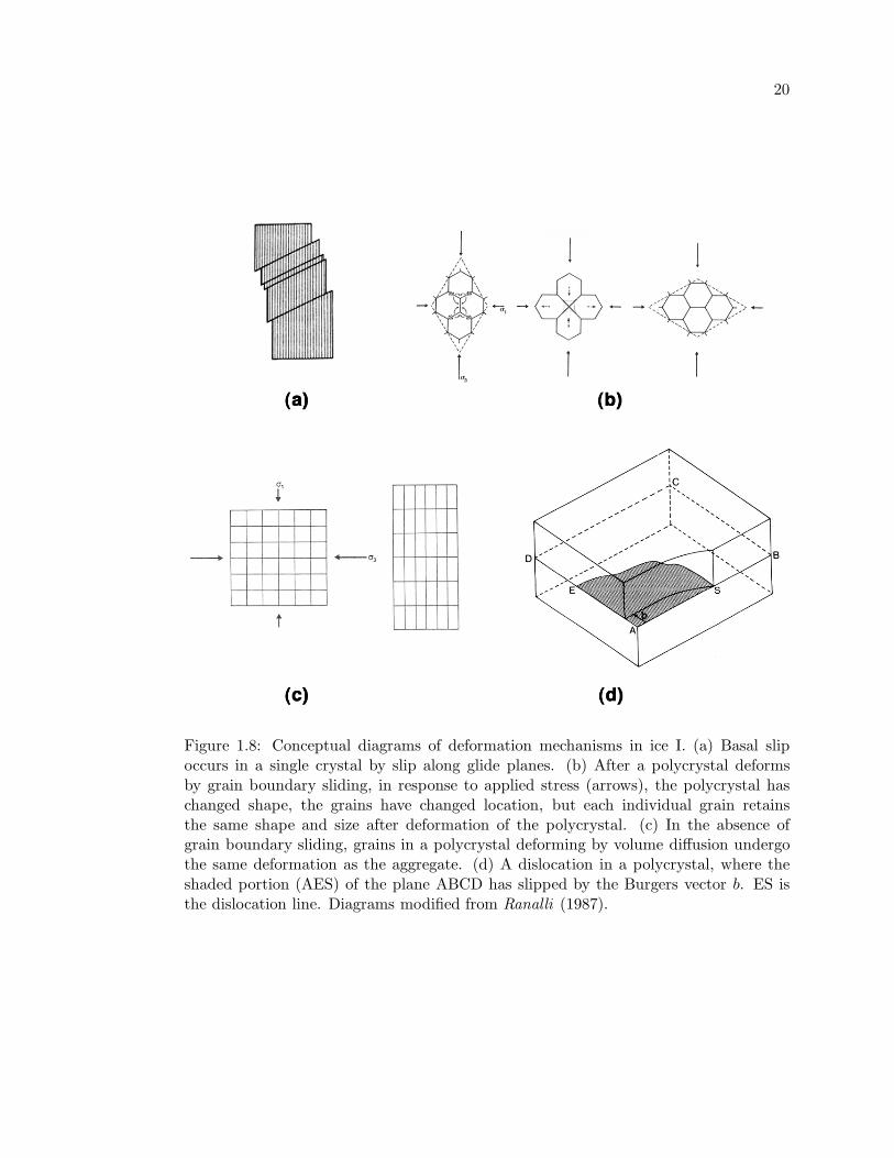
diagrams of the four deformation mechanisms are shown in Figure 1.8.

The total rate of deformation in ice I is expressed as the sum of strain rates due

to the four individual creep mechanisms,

εtotal = εdiff + εdisl +

(

1

εGBS+

1

εbs

)−1

, (1.4)

where (diff) represents diffusional flow, (disl) represents dislocation creep, (bs) rep-

resents basal slip, and GBS represents grain boundary sliding. Grain boundary slid-

ing and basal slip (collectively, grain-size-sensitive creep, or GSS creep) are dependent

mechanisms, and both must operate simultaneously to permit deformation (Durham

and Stern, 2001).

The strain rate for each deformation mechanism is described by

ε = Aσn

dpexp

(−Q∗

RT

)

, (1.5)

where ε is the strain rate, A is the pre-exponential parameter, σ is stress, n is the stress

exponent, d is the ice grain size, p is the grain size exponent and Q∗ is the activation

energy, R is the gas constant, and T is temperature. Rheological parameters from the

experiments of Goldsby and Kohlstedt (2001) used in our models are summarized in

Table A.2.

For ice near its melting point, Goldsby and Kohlstedt (2001) present an alternate

set of creep parameters to describe large creep rates and low viscosities observed in ice

near its melting point in terrestrial ice cores and laboratory samples. The enhancement

of creep rates in ice near its melting point is attributed to premelting along grain

boundaries and edges. High temperature creep enhancement is not included in the

models presented in this thesis, but the possible implications of including such a term,

are discussed when relevant, in Chapters 2, 3, 4, and 6.

The deformation mechanism that yields the highest strain rate for a given tem-

perature and differential stress is judged to dominate flow at that temperature and

20

Figure 1.8: Conceptual diagrams of deformation mechanisms in ice I. (a) Basal slipoccurs in a single crystal by slip along glide planes. (b) After a polycrystal deformsby grain boundary sliding, in response to applied stress (arrows), the polycrystal haschanged shape, the grains have changed location, but each individual grain retainsthe same shape and size after deformation of the polycrystal. (c) In the absence ofgrain boundary sliding, grains in a polycrystal deforming by volume diffusion undergothe same deformation as the aggregate. (d) A dislocation in a polycrystal, where theshaded portion (AES) of the plane ABCD has slipped by the Burgers vector b. ES isthe dislocation line. Diagrams modified from Ranalli (1987).

21

stress level. The transition stress between any pair of flow laws, for example, GBS and

dislocation creep, is

σT =

(

AGBS

Adisl

dpdisl

dpGBSexp

((Q∗

disl − Q∗GBS)

RT

))1

ndisl−nGBS

. (1.6)

The expressions for the transition stresses between the various deformation mechanisms

can be used to construct deformation maps showing the boundaries of regimes of domi-

nance for each constituent creep mechanism. Deformation maps for ice with grain sizes

0.1 mm, 1.0 mm, 1.0 cm, and 10 cm are shown in Figure 3.1. If the high-temperature

creep enhancement is not included in the rheology, deformation in ice is accommodated

by the Newtonian deformation mechanism of volume diffusion when the temperature of

the ice is close to the melting point, or the grain size is small, (d < 1 mm). In this regime

of behavior, the viscosity of ice depends strongly on temperature only. At lower temper-

atures and/or for grain sizes larger than 1.0 cm, deformation in ice is accommodated by

dislocation creep, and the viscosity of ice depends strongly on temperature and stress.

For intermediate grain sizes, deformation occurs due to GSS creep, and the viscosity of

the ice is strongly temperature-dependent, but only weakly stress-dependent.

1.5 Convection in Ice I

Over millions of years, the behavior of ice can be described as flow of a highly

viscous fluid, analogous to flow within the Earth’s mantle. The outer ice I shells of large

icy satellites are heated from beneath by decay of radioactive elements in the satellites’

rocky interiors, and potentially from within by tidal dissipation. Similar to rock, ice

expands when it is heated, so a basally heated or internally heated ice shell will be

gravitationally unstable, and when perturbed, warm ice will rise from the base of the

shell. Likewise, cold pockets of ice near the surface will sink. When this process is self-

sustaining over a geologically long time scale, it is referred to as solid-state convection.

22

1.5.1 Governing Equations

In this work, the outer ice I shells of the Galilean satellites are approximated as

2D Cartesian plane layers of incompressible fluids. The outer ice I shells occupy a small

fraction of the total radii of the satellites, so treating the shells as plane layers of fluid is

a valid approximation. The equations of convection are phrased in the Boussinesq ap-

proximation, where small density differences due to thermal expansion drive convective

motion.

Conservation of mass in thermal convection is expressed by the continuity condi-

tion (Schubert et al., 2001):

∇ · ~v = 0, (1.7)

where ~v = (vx, vz) is the velocity field. Physically, equation (1.7) dictates that no

sources or sinks of material exist in the fluid layer. Conservation of energy in thermal

convection is expressed by

~v · ∇T︸︷︷︸

Advection

+∂T

∂t= κ∇2T

︸︷︷︸

Diffusion

+ γ︸︷︷︸

Sources

, (1.8)

where T is temperature, t is time, κ is the thermal diffusivity, and γ represents external

heat sources such as radiogenic heating in the interior of the fluid layer (Schubert et al.,

2001). In this work, γ = 0. In the convecting fluid, energy is transfered by mass

transport (advection) in addition to thermal diffusion. Conservation of momentum (i.e.

force balance) is described by:

−∇P + ρgez︸︷︷︸

Hydrostatic Equilibrium

= −∇ · [η(∇~v + ∇T~v])︸︷︷︸

Viscous Forces

(1.9)

where P is pressure, ρ is the density of the fluid, g is gravity, ez is a unit vector in the z-

direction, and η is the fluid viscosity (Schubert et al., 2001). In the convecting layer, the

viscous forces act against thermal buoyancy to retard upward motion of warm fluid and

downward motion of cold fluid. Thermal buoyancy is introduced into the momentum

23

balance equation by substituting

ρ = ρo[1 − α(T − To)], (1.10)

where ρo is the density of the fluid at a reference temperature (To) and α is the coeffi-

cient of thermal expansion, into equation (1.9). Lithostatic pressure is eliminated from

equation (1.9) by substituting

P = ρogez − p, (1.11)

where p is the dynamic pressure. With these substitutions, equation (1.9) becomes:

∇p + ρoα(T − To)gez = ∇ · [η(∇~v + ∇T~v)]. (1.12)

It is helpful to notice at this point that the only time dependence in the governing

equations appears in the advection-diffusion terms in equation (1.8), and the momen-

tum balance equation (1.12) is time-independent. This occurs because the viscosity

of the ice is very large, so thermal diffusion dominates over diffusion of momentum

through the fluid by viscous flow. Fluid velocities therefore change very slowly with

time. Mathematically, the Navier-Stokes equation (Kundu, 1990):

∂vi

∂t+ vj

∂vi

∂xj=

−1

ρ

∂p

∂xi+ gez , (1.13)

reduces to

vj∂vi

∂xj=

−1

ρ

∂p

∂xi+ gez (1.14)

because

∂vi

∂t∼ 0, (1.15)

and is independent of time. Equation (1.14) is essentially the same as equation (1.12).

In this study, the equations of thermal convection (1.7), (1.8), and (1.12) are

solved subject to constant temperature boundary conditions at the surface and base of

the fluid layer,

T (x,−D) = Tm (1.16)

T (x, 0) = Ts, (1.17)

24

and insulating edges

∂T

∂x

∣∣∣∣x=xmax

= 0. (1.18)

Free-slip (zero shear stress) boundary conditions are imposed at the edges of the fluid

layer:

∂vz

∂x

∣∣∣∣x=0,xmax

= 0 (1.19)

and on the top and bottom surfaces of the layer,

∂vx

∂z

∣∣∣∣z=0,−D

= 0 (1.20)

An initial condition of form:

T (x, z) = Ts −z∆T

D+ δT cos

(2πD

λx

)

sin

(−zπ

D

)

(1.21)

is used, where δT and λ are the amplitude and wavelength of the perturbation, and z =

−D at the warm base of the ice shell. The temperature field defined by equation (1.21)

represents the sum of the temperature field resulting from a conductive equilibrium

between the surface and base of the ice shell, and a temperature anomaly, distributed

according to:

δT (x, z) = δT cos

(2πD

λx

)

sin

(−zπ

D

)

. (1.22)

Figure 1.9 illustrates a temperature anomaly (δT (x, z)) of amplitude 15 K in an ice shell

30 km thick used in a simulation in this thesis.

The finite element model Citcom developed to study convection in terrestrial plan-

etary mantles is used in this study to solve equations (1.7), (1.8), and (1.12) subject

to the boundary conditions described above. A general overview of the finite element

method can be found in Hughes (1987). The momentum equation and continuity equa-

tions are solved using a Uzawa algorithm (Ramage and Wathen, 1994), and a Streamline

Upwind Petrov-Galerkin method is used to solve the energy equation (Brooks, 1981).

Details regarding the specific implementation of these techniques in Citcom to solve

25

-30

-20

-10

0D

epth

(km

)

0 10 20

X (km)

-15 -10 -5 0 5 10 15

δT (K)

Figure 1.9: Initial temperature perturbation issued to the ice shell (δT (x, z)) from asample simulation in this thesis. Here, Ts = 110 K and Tm = 260 K, so δT = 0.1∆T=15K. The wavelength of perturbation used here is λ = 1.75D. The temperature excess anddeficit that trigger convection in the ice shell are spaced approximately 27 km apart.

26

the governing equations of convection and application of Citcom to terrestrial planetary

problems can be found in Moresi and Gurnis (1996), Zhong et al. (1998), and Zhong

et al. (2000).

Given an initial temperature field, Citcom generates a velocity field based on the

viscosity of the ice, thermal buoyancy, and conservation of momentum. The dynamic to-

pography from convection and heat flux are calculated, after which the energy equation

is solved and the solution is propagated forward in time.

The temperature and velocity fields are defined at each computational node, and

the dynamic topography and heat flux at the surface and base of the convecting layer

are output after a number of time steps. In addition to the total viscosity field, when im-

plementing a composite rheology for ice I in Chapters 3 through 5, Citcom is instructed

to report an effective viscosity due to each individual creep mechanism (diffusional flow,

GSS creep, and dislocation creep). This information is used to judge the relative impor-

tance of each deformation mechanism in accommodating convective strain in Chapters

3 and 4.

1.5.2 Non-Dimensional Coordinates

Within the framework of Citcom, the equations of thermal convection are solved

in non-dimensional coordinates. The coordinates are non-dimensionalized using the

Rayleigh number, a ratio between the thermal buoyancy and viscous restoring forces in

the fluid:

Ra =ρgα∆TD3

κηo, (1.23)

where ∆T is the temperature difference between the surface and bottom of the layer,

D is the thickness of the layer, and ηo is the reference viscosity. The reference value of

Rayleigh number supplied to Citcom determines the quantities used to re-dimensionalize

the coordinates after the simulation is complete. When the viscosity is dependent on

temperature and strain rate (or stress), the Rayleigh number of the fluid layer becomes

27

a function of temperature and strain rate (or stress), necessitating a precise definition of

the Rayleigh number in terms of a reference temperature and strain rate (or stress). In

this thesis, the Rayleigh number is always defined at the melting temperature of ice. A

reference strain rate εo = κD2 is used in Chapter 2. In Chapters 3 through 5, a reference

strain rate of εo = 10−13 s−1 is used, largely for algebraic convenience.

The definition of the reference strain rate, and thus, the reference Rayleigh num-

ber, is somewhat arbitrary, so the values of Rayleigh number used in simulations with

a composite rheology for ice I may seem counterintuitive (for example, Rao = 10−2)

when the grain size of ice is large and the ice becomes strongly non-Newtonian. In a

non-Newtonian fluid, as the fluid begins to flow and convection starts, the viscosities in

the fluid layer decrease. The viscosity in the convecting sublayer may be several orders

of magnitude lower than the reference viscosity. A more physically intuitive definition

of Rayleigh number in the non-Newtonian case is the effective Rayleigh number:

Raeff =Raoηo

〈η〉(1.24)

where the average viscosity in the convecting sublayer (〈η〉) can be calculated after the

convection simulation is run.

The temperature in the fluid layer is rephrased in non-dimensional coordinates

(primed quantities) using the temperature difference between the base of the ice layer

and the surface of the layer,

T ′ =T − Ts

Tm − Ts, (1.25)

where Tm is the melting temperature of ice, and Ts is the surface temperature on the

icy satellite. The warm base of the ice shell at z = −D is held at a non-dimensional

temperature T ′ = 1, and the surface is held at T ′ = 0. The spatial coordinates in the

fluid layer are non-dimensionalized using the thickness of the ice shell,

x′ =x

D(1.26)

z′ =z

D. (1.27)

28

Time coordinates (t) and velocity coordinates (v) are non-dimensionalized using the

thermal diffusivity and layer thickenss as:

t′ =tD2

κ(1.28)

v′ =vD

κ. (1.29)

The dynamic topography resulting from thermal bouyancy is output in units of pressure,

which can be converted to heights using p = ρgh as:

htopo =p′ηoκ

ρgD2. (1.30)

Mass fluxes (M = ρv2) due to convection are re-dimensionalized using

M = ρ(v′)2κD, (1.31)

where an implicit assumption has been made that the structure of the convective flow

field in the third (unsued) y dimension, is identical to the x direction.

1.5.3 Viscosity Functions

A series of temperature-, strain rate-, and stress-dependent viscosity functions

for ice I are implemented in Citcom to allow the model to apply to icy satellites. In

this thesis, the temperature dependence in the ice flow laws are expressed using an

Arrhenius law, which is common practice for icy satellite studies. In this formulation,

the lab-derived flow law of form

η(T ) = A exp( Q∗

nRT

)

, (1.32)

is non-dimensionalized by dividing by the viscosity evaluated at the melting point,

η′(T ′) = exp

(E

T ′ + T ′o

−E

1 + T ′o

)

, (1.33)

where E = Q∗/nR∆T and T ′o = Ts/∆T . This procedure retains the exact temperature

dependence determined by laboratory experiments, and predicts very large viscosities

29

near the surface of the ice shell. In this study, numerical cut-offs to limit the viscosity

values near the surface of max(η) = 107 − 1010 are used to prevent essentially infinite

viscosities in the near-surface ice.

In Chapter 2, a single term from the composite rheology for ice I (equation 1.4)

for grain boundary sliding or basal slip is implemented. The viscosity due to GBS or

basal slip in ice is calculated as a strain rate-dependent viscosity,

η =

(dp

A

)1/n

ε(1−n)/nII exp

(Q∗

nRT

)

, (1.34)

where εII is the second invariant of the strain rate tensor:

εII =1

2

(∑

i,j

(∂vi

∂vj+

∂vj

∂vi

))1/2. (1.35)

This form of viscosity function approximates the behavior of a true stress-dependent

rheology, but is more numerically tractable in Citcom than a stress-dependent viscosity

function.

When the viscosity is stress- or strain rate-dependent, the velocity and viscosity

fields are coupled. The fields must be solved iteratively until convergence is achieved.

This introduces further non-linearity to the convection problem and can result in very

low viscosities in the convecting region where the ice is flowing, and large viscosities in

the near surface ice where convective motions are negligible. The requirement to iterate

to find self-consistent viscosity and velocity fields makes simulations of convection in

non-Newtonian fluids computationally expensive compared to Newtonian models. As a

result, before this thesis, implementation of the strain rate- or stress-dependence has so

far been ignored in numerical convection models of icy satellites.

1.5.4 Composite Rheology for Ice I

The full composite rheology for ice I (equation 1.4) is implemented in simulations

presented in Chapters 3, 4, and 5. In the composite rheology determined by Goldsby

30

and Kohlstedt (2001), each deformation mechanism has a distinct stress exponent and

activation energy, so inversion of equation (1.4) for an exact expression for viscosity

(η = σ/ε) is not possible. However, an approximate expression for the viscosity due to

all four deformation mechanisms can be found using the procedure described here.

The composite flow law for ice I (equation 1.4) can be expressed in terms of

stresses using η = σ/ε as

σtot

ηtot=

σdiff

ηdiff+

σdisl

ηdisl+

(

ηGBS

σGBS+

ηbs

σbs

)−1

. (1.36)

With the approximation that the stresses for each deformation mechanism are

approximately equal to the total stress (i.e., σtot = σdiff = σGBS = σbs), equation

(1.36) can be re-written as:

σtot

(

1

ηtot

)

∼ σtot

[

1

ηdiff+

1

ηdisl+

(

ηGBS + ηbs

)−1]

. (1.37)

Canceling the common factor of σtot, the expression for the approximate viscosity

due to all four mechanisms becomes

1

ηtot=

[

1

ηdiff+

1

ηdisl+

(

ηGBS + ηbs

)−1]

. (1.38)

The approximate nature of this expression is most evident near the transition stresses

between pairs of deformation mechanisms, where the viscosity is underestimated. If the

stress applied to the ice is much larger than the transition stresses between the pairs

of deformation mechanisms, a single term in the composite flow law will contribute the

majority of the total strain rate, so the viscosity may be calculated using η = σ/ε by

assuming the contribution of the other terms are negligible. At the transition stress

between a pair of mechanisms, each mechanism contributes to the strain rate equally,

and errors are introduced by neglecting the contribution from one of the constituent

mechanisms. This effect is demonstrated graphically in Figure 3.2.

A stress dependent rheology of form

η =dp

Aσ(1−n) exp

( Q∗

RT

)

, (1.39)

31

is used for each term in the composite rheology (equation 1.38). The resulting flow law

for ice I is

1

ηtot=

Adiff

d2exp

(−Q∗

v

RT

)

+ Adislσ3 exp

(−Q∗

disl

RT

)

+

+

(

d1.4

AGBSσ−0.8 exp

(Q∗

GBS

RT

)

+1

Absσ−1.4 exp

(Q∗

bs

RT

))−1

(1.40)

where the stress and grain size exponents for each flow law have been evaluated to

highlight the weakly non-Newtonian behavior of grain boundary sliding and basal slip.

To non-dimensionalize the viscosity functions, each term in the composite rheol-

ogy (equation 1.38) is divided by a reference viscosity defined by the viscosity due to

diffusion creep at the melting temperature of ice. The strain rate from diffusion creep

is described by

ε =ADF Vmσ

RTmd2

(

Dv +πδ

dDb

)

(1.41)

where ADF is the diffusion constant, Vm is the molar volume, Tm is the melting tem-

perature of ice, Dv is the rate of volume diffusion, δ is the grain boundary width, and

Db is the rate of grain boundary diffusion. For small strains of order 1%, ADF = 42,

but for larger strains ADF > 42 (Goodman et al., 1981). Here, ADF = 42 is used.

The grain sizes of ice in the satellites are likely much larger than the grain bound-

ary width (9.04×10−10 m) (Goldsby and Kohlstedt , 2001), so volume diffusion dominates

over grain boundary diffusion, and the contribution to the strain rate by grain boundary

diffusion is negligible. The strain rate for volume diffusion is:

ε =42Vmσ

RTmd2Do,v exp

(−Q∗

v

RT

)

(1.42)

where Do,v is the volume diffusion rate coefficient and Q∗v is the activation energy.

The parameters for volume diffusion are listed in Table A.2, where the pre-exponential

parameters have been grouped as A = (42VmDo,v/RTm). The viscosity due to volume

diffusion is, therefore,

ηo =d2

Aexp

( Q∗v

RTm

)

. (1.43)

32

The non-dimensionalized form of the composite viscosity (equation 1.40) is,

1

ηtot= exp

(Ev

1 + T ′o

−Ev

T ′ + T ′o

)

+ βdislσ′3 exp

(−Edisl

T ′ + T ′o

)

+

(

βGBSσ′−0.8 exp

(EGBS

T ′ + T ′o

)

+ βbsσ′−1.4 exp

(Ebs

T ′ + T ′o

))−1

, (1.44)

where Ei = Q∗i /R∆T .

The transition stresses between the various deformation mechanisms are repre-

sented in the expression for total viscosity by a series of relative weighting factors (β)

between the four rheologies, which govern the relative importance of each deforma-

tion mechanism as a function of temperature and grain size. The weighting factor for

dislocation creep is given by

βdisl = Adislη3o ε

−4o , (1.45)

where ηo is the reference viscosity, εo = 10−13 s−1 is the reference strain rate. The

weighting factors for GBS and basal slip are

βGBS =d1.4

AGBSη−1.8

o ε−0.8o (1.46)

and

βbs =1

Absη−2.4

o ε−1.4o . (1.47)

Values of the weighting factors for each rheology are shown in Table B.7 for the range

of grain sizes used.

Information about the stress field (σ = ηε) is not available to Citcom when the

viscosity subroutine is accessed because only the velocity field is known. Following the

suggestion of Allen McNamara (personal communication), who implemented composite

rheologies for mantle materials in McNamara et al. (2003), a subroutine to calculate

the stress iteratively using σ = ηεII was implemented. This procedure permits use of a

stress-dependent rheology, but introduces a further iterative loop in the solution, which

makes implementation of a stress-dependent composite rheology more computationally

expensive than a strain rate-dependent rheology.

33

Regardless of which type of viscosity function is implemented, a smoothing al-

gorithm is applied to to the viscosity field between time steps. This technique was

suggested by Jeroen Van Hunen (personal communication) after it was discovered that

an Arrhenius temperature law and strain rate-dependent viscosity subroutines caused

wild swings in the viscosity field between time steps in the particular version of Citcom

used in this thesis. After the viscosity subroutine is called, the viscosity information is

saved, and in the next time step, the new viscosity and old viscosity are averaged using

ln(ηnew) = (1 − w) ln(ηold) + w ln(ηnew), (1.48)

where w = 0.2 is a weighting factor.

1.6 The Onset of Convection

Whether convection can occur in an ice layer is governed by the relative balance of

thermal buoyancy forces to viscous restoring forces in the ice. The stability of a basally

heated fluid layer against convection can be judged by examining the balance between

thermal buoyancy, which drives the formation of plumes at the base of the fluid layer,

thermal diffusion, which acts to decrease thermal buoyancy, and the viscous restoring

forces that retard plume growth. The balance of forces against thermal diffusion is

expressed by the Rayleigh number, and convection can occur in a fluid layer if the

Rayleigh number of the fluid layer exceeds a critical value (Racr) which depends on the

wavelength of initial temperature perturbation issued to the layer and the geometry of

the layer.

1.6.1 Linear Stability Analysis

The onset of thermal convection in fluids is commonly modeled using the tech-

nique of linear stability analysis (Chandrasekhar , 1961; Turcotte and Schubert , 1982),

in which the growth or decay of an initial temperature perturbation embedded in a con-

34

ductive fluid layer is analyzed to determine the critical Rayleigh number for convection.

If the amplitude of an initial perturbation grows with time, the fluid layer can convect.

If the amplitude decays and the layer returns to a conductive equilibrium, the fluid layer

cannot convect.

The gravitational restoring forces that retard plume growth depend on the vis-

cosity of the fluid, so the critical Rayleigh number is a function of the rheology of the

fluid in addition to the thermal and physical properties of the fluid layer. For a fluid

with a viscosity dependent on temperature only, the critical Rayleigh number is a func-

tion of how sharply the viscosity varies with temperature near the melting point. In a

fluid with a non-Newtonian rheology, the restoring force depends on the thermal stress

generated by the initial convecting plume. As a result, the critical Rayleigh number for

convection in a non-Newtonian fluid depends on the initial temperature perturbation in

the fluid, in addition to the rheological and physical parameters.

1.6.2 Non-Newtonian Rheologies

Numerical studies regarding the onset of convection in non-Newtonian, basally

heated fluids define the critical Rayleigh number as the minimum value of Rayleigh num-

ber where convection cannot occur regardless of initial conditions (Solomatov , 1995).

This definition of critical Rayleigh number is directly relevant to terrestrial planets be-

cause it can be used to address the conditions under which convection in a planetary

mantle will cease as the radiogenic heating that drives convection in terrestrial planets

decays with time.

However, the critical Rayleigh number for the onset of convection in a non-

Newtonian fluid cannot be determined using linear stability analysis (Tien et al., 1969;

Solomatov , 1995). The viscosity of a non-Newtonian fluid depends on both temper-

ature and strain rate, so the viscosity in the perturbed layer of fluid depends on the

amplitude of the initial perturbation and becomes infinite as the amplitude becomes

35

small (Solomatov , 1995). Convection in a non-Newtonian fluid with a temperature- and

strain rate-depdendent rheology is always a finite-amplitude instability, and cannot be

readily analyzed analytically (Solomatov , 1995).

Analysis of the onset of convection in a fluid with stress-dependent (but not

temperature-dependent) rheology can provide constraints on how the non-Newtonian

behavior affects Racr. An alternative method of determining Racr for a non-Newtonian

fluid stems from a physical argument put forth by Chandrasekhar (1961), who pos-

tulated that the critical Rayleigh number occured at a critical temperature gradient

where the dissipation of energy by viscous forces in the system exactly balanced the

release of energy from the rising, thermally buoyant plume. Using an energy balance

argument, Tien et al. (1969) were able to calculate the critical Rayleigh number for

non-Newtonian fluids with a range of values of stress exponent, which compared fa-

vorably to their laboratory measurements of critical Rayleigh number for fluids with

stress-dependent rheologies.

The most widely-used results for the critical Rayleigh number for convection in a

non-Newtonian fluid arise from the pivotal study of Solomatov (1995), who built upon

the analysis of Tien et al. (1969) plus additional studies by Ozoe and Churchill (1972)

to consider a stress- and temperature-dependent rheology. With the knowledge that

the critical Rayleigh number for a non-Newtonian fluid depends on initial conditions,

Solomatov (1995) characterized the value of Rayleigh number where convection could

not occur, regardless of initial conditions.

Unlike terrestrial planets, icy satellites can potentially receive bursts of heat due

to tidal dissipation relatively late in their evolutionary histories. If an ice shell is con-

vecting when tidal dissipation begins, and the heat generated within the ice exceeds the

maximum convective heat flux, which is controlled by the rheology of ice, the shell will

melt at its base and thin. If the layer thickness drops below a critical value, convection

will cease. The value of critical layer thickness where convection is no longer possible

36

can be estimated using the Rayleigh number characterized by terrestrial studies, for

example, Solomatov (1995). However, if the ice shell is in conductive equilibrium when

tidal dissipation begins, the viscosity of the motionless ice would be large, and a large

temperature anomaly would be required to soften the non-Newtonian ice layer enough

to permit convection.

A loosely analogous situation can occur on Earth, beneath the continents where

thickened non-Newtonian lithosphere can become gravitationally unstable and form

plumes that sink into the mantle. Numerical simulations and experiments suggest that

the growth rate of lithospheric thickness perturbations depends on a power law of the

perturbation amplitude (Molnar et al., 1998). Thus, the critical Rayleigh number for

the onset of sublithospheric convection depends on a power of the perturbation ampli-

tude. Calculations presented in Chapters 2 and 3 will show that the critical Rayleigh

number for convection in non-Newtonian ice is strongly dependent on the physical char-

acteristics of the temperature anomalies within the ice shell, specifically their amplitude

and wavelength.

1.7 Previous Studies of Convection in the Icy Satellites

A large volume of literature exists regarding convection in the outer ice I shells of

the icy Galilean satellites, dating back to the pre-Voyager study of Reynolds and Cassen

(1979). The studies fall into two broad categories: parameterized convection models,

and numerical convection models. Parameterized convection studies use algebraic scal-

ing laws between the thermal and physical properties of the ice, the critical Rayleigh

number, and the convective heat flux to determine whether convection occurs, and the

efficiency of convective heat transfer.

Modern applications of parameterized convection models such as Spohn and Schu-

bert (2003) and Ruiz (2001) focus on determining the conditions under which the liq-

uid water oceans can remain stable against convective and conductive heat transport.

37

At the heart of such studies are the relationships between the critical Rayleigh num-

ber and the rheology of ice, and the Rayleigh number - Nusselt number relationship,

which expresses the efficency of convective heat transport. Both relationships are highly

rheology-dependent.

Results of many numerical studies designed for terrestrial mantle convection such

as Solomatov (1995) and Solomatov and Moresi (2000) have been brought to bear on

the critical Rayleigh number and the Ra-Nu scaling. In general, parameterized studies

predict that oceans are not thermodynamically stable beneath a convecting ice shell,

due to efficient convective heat transport. The results of these studies are limited by

uncertainties in the rheology of ice and the role of tidal dissipation. The majority

of these studies have been conducted with Newtonian rheologies for ice I, but recent

works regarding convection in Europa’s ice I shell by Nimmo and Manga (2002) and the

convective stability of Callisto’s ice I shell by Ruiz (2001) use individual non-Newtonian

terms from the Goldsby and Kohlstedt (2001) rheology.

Numerical studies such as this thesis typically involve implementing rheologies

for ice I in a finite-element convection model with the goal of refining the algebraic laws

used in parameterized studies. Numerical studies have recently come into favor as a tool

for addressing the formation of surface features on Europa (Tobie et al., 2003; Showman

and Han, 2004).

Numerical simulations of convection in ice I have so far been limited to Newtonian

rheologies. Most of the numerical efforts have focused on implementing a model for tidal

dissipation in the ice shell developed by Wang and Stevenson (2000), extended by Tobie

et al. (2003) and Showman and Han (2004). The non-Newtonian behavior of ice I has

been ignored in previous convection models, with the rationale that the viscosity of ice

is only weakly stress-dependent, so the temperature-dependence dominates the behavior

of the ice shell. The results presented in Chapter 4 indicate that when studying well-

developed convection patterns in ice, this assumption is largely true. However, a key

38

and significant departure between Newtonian and non-Newtonian convection in ice I

occurs in the onset of convection, which will be discussed in detail in Chapters 2 and 3.

Chapter 2

Convective Instability in Ice I with Non-Newtonian Rheology

This chapter is in press in the Journal of Geophysical Research:

Barr, A. C., R. T. Pappalardo, S. Zhong (2004), Convective Instability in Ice I

with Non-Newtonian Rheology: Application to the Icy Galilean Satellites, J. Gephys.

Res., 2004JE002296, in press.

2.1 Abstract

At the temperatures and stresses associated with the onset of convection in an ice

I shell of the Galilean satellites, ice behaves as a non-Newtonian fluid with a viscosity

that depends on both temperature and strain rate. The convective stability of a non-

Newtonian ice shell can be judged by comparing the Rayleigh number of the shell

to a critical value. Previous studies suggest that the critical Rayleigh number for a

non-Newtonian fluid depends on the initial conditions in the fluid layer, in addition

to the thermal, rheological, and physical properties of the fluid. We seek to extend

the existing definition of the critical Rayleigh number for a non-Newtonian, basally

heated fluid by quantifying the conditions required to initiate convection in an ice I

layer initially in conductive equilibrium. We find that the critical Rayleigh number for

the onset of convection in ice I varies as a power (-0.6 to -0.5) of the amplitude of the

initial temperature perturbation issued to the layer, when the amplitude of perturbation

is less than the rheological temperature scale. For larger amplitude perturbations, the

40

critical Rayleigh number achieves a constant value. We characterize the critical Rayleigh

number as a function of surface temperature of the satellite, melting temperature of

ice, and rheological parameters so that our results may be extrapolated for use with

other rheologies and for a generic large icy satellite. The values of critical Rayleigh

number imply that triggering convection from a conductive equilibrium in a pure ice

shell less than 100 km thick in Europa, Ganymede, or Callisto requires a large, localized

temperature perturbation of 1-10’s K to soften the ice, and therefore may require tidal

dissipation in the ice shell.

2.2 Introduction

Results from the Galileo magnetometer strongly suggest the presence of liquid

water oceans within Jupiter’s satellites Europa, Ganymede, and Callisto (Zimmer et al.,

2000; Kivelson et al., 2002). Measurements of Europa’s gravitational field indicate that

the outer 170 km of the satellite is composed of H2O-rich material, which may be in some

part liquid (Anderson et al., 1998). Because the density of liquid water is intermediate

between the densities of ice I and its high pressure polymorphs, liquid water oceans

within Ganymede and Callisto are likely sandwiched between layers of ice I atop the

ocean and ice III or V beneath the ocean. The modes of heat transport in the ice shells

and their methods of endogenic resurfacing are not well understood, in part because

uncertainties in the shell thickness, the rheology of ice, and the role of tidal dissipation

hamper efforts to judge whether the ice shells convect.

The onset of convection is commonly modeled using the technique of linear sta-

bility analysis (Chandrasekhar , 1961; Turcotte and Schubert , 1982), where the balance

of forces acting on a temperature anomaly embedded in an initially conductive fluid

layer is analyzed to determine the conditions under which the anomaly will grow, thus

initiating convection in the layer.

41

The balance of forces in the fluid is expressed by the Rayleigh number,

Ra =ρgα∆TD3

κη, (2.1)

where ρ is the density of the fluid, g is the acceleration of gravity, α is the coefficient

of thermal expansion, ∆T is the temperature difference between the surface and the

bottom of the convecting layer, κ is the thermal diffusivity, and η is the fluid viscosity.

Convection can begin if the Rayleigh number of the ice shell exceeds the critical Rayleigh

number (Racr). For ice with a temperature-dependent viscosity, the critical Rayleigh

number is a function of the rheology of the ice, the boundary conditions used in the

model of the ice shell, and the wavelength of the initial convective upwelling.

A large volume of experimental data and observations exist regarding the rheol-

ogy of ice I in terrestrial and planetary contexts (Durham and Stern, 2001 and references

therein). Recent laboratory experiments seeking to clarify the deformation mechanisms

responsible for flow in terrestrial ice sheets suggest that a composite flow law which

includes terms due to diffusional flow, grain boundary sliding, basal slip, and disloca-

tion (Goldsby and Kohlstedt , 2001) creep can match both viscosity measurements from

terrestrial ice sheets (Peltier et al., 2000) and previous laboratory experiments.

The deformation mechanisms that accommodate large convective strains in ice

I and their governing parameters appropriate for the icy Galilean satellites are by no

means certain. However, because so many of the governing parameters of icy satellite

convection are poorly constrained, we study the implications of the flow law determined

by Goldsby and Kohlstedt (2001) for convection in the outer ice I shells of the Galilean

satellites, paying particular attention to the non-Newtonian behavior of ice, which has

not been widely employed in previous models of the satellites.

If the ice shell has a grain size of order 1 mm, the strain associated with growing

convective plumes in an ice shell in the Galilean satellites is accommodated by grain

boundary sliding and basal slip, which yield non-Newtonian viscosities for ice dependent

42

on temperature and stress. As a result, the viscous restoring force retarding plume

growth depends on strain rate. Therefore, the critical Rayleigh number is a function of

the initial conditions in the ice shell in addition to the ice rheology, boundary conditions,

and wavelength of convective upwelling.

Numerical studies regarding the onset of convection in a non-Newtonian, basally

heated fluid layer define the critical Rayleigh number as the minimum value of Rayleigh

number where convection cannot occur regardless of initial conditions (Solomatov, 1995

and references therein). This definition of Rayleigh number is directly relevant to terres-

trial planets because it can be used to address the conditions under which convection in

a planetary mantle will cease as the radiogenic heating that drives convection decreases

with time.

Unlike terrestrial planets, icy satellites can receive bursts of heat due to tidal

dissipation relatively late in their evolutionary histories. If an ice shell is convecting

when tidal dissipation begins, and the heat generated within the ice exceeds the max-

imum convective heat flux, which is controlled by the ice rheology, the shell will melt

at its base and thin. If the layer thickness drops below a critical value, convection will

cease. The value of critical layer thickness where convection is no longer possible can be

estimated using the Rayleigh number characterized by Solomatov (1995). However, if

the ice shell is in conductive equilibrium when tidal dissipation begins, the viscosity of

the motionless ice would be large, and a large temperature anomaly would be required

to soften the non-Newtonian ice layer enough to permit convection.

A loosely analogous situation can occur on Earth, beneath the continents where

thickened non-Newtonian lithosphere can become gravitationally unstable and form

plumes that sink into the mantle. Numerical simulations and experiments suggest that

the growth rate of lithospheric thickness perturbations depends on a power law of the

perturbation amplitude (Molnar et al., 1998). Thus, the critical Rayleigh number for

the onset of sublithospheric convection depends on a power of the perturbation am-

43

plitude. We can expect, therefore, that the critical Rayleigh number for convection

in non-Newtonian ice will be strongly dependent on the physical characteristics of the

temperature anomalies within the ice shell, specifically their amplitude and wavelength.

To determine the conditions required to trigger convection from a conductive

equilibrium in a non-Newtonian ice I shell, we determine the critical Rayleigh number for

the onset of self-sustaining convection in ice with grain boundary sliding and basal slip

rheologies, for a range of initial conditions. We develop an algebraic relationship between

the critical Rayleigh number and the initial conditions within the ice shell, surface

temperature of the satellite, melting temperature of ice, and rheological parameters so

that our results may be extrapolated for use with other rheologies or within a generic

large pure-water-ice satellite. We use this scaling between critical Rayleigh number,

initial conditions, and rheological parameters to determine what conditions are required

to trigger convection in conductive ice shells in Europa, Ganymede, and Callisto.

2.3 Methods

2.3.1 Numerical Implementation of Ice I Rheology

The laboratory experiments of Goldsby and Kohlstedt (2001) characterize creep

in ice I due to four different deformation mechanisms resulting in a composite flow law,


(

1

εbs+

1

εGBS

)−1

. (2.2)

The composite flow law includes contributions from diffusional flow (diff ), disloca-

tion creep (disl), and grain-size-sensitive creep (GSS), where deformation occurs by

both grain boundary sliding-accommodated basal slip (bs, basal slip) and basal slip-

accommodated grain boundary sliding (GBS) (Goldsby and Kohlstedt , 2001). Basal slip

and GBS are dependent mechanisms and both must operate simultaneously to permit

deformation. When responsible for flow, the total strain rate for GSS is controlled by

the slower of the two mechanisms (Durham and Stern, 2001).

44

The strain rate for each creep mechanism in the composite rheology is described

by

ε = Aσn

dpexp

(−Q∗

RT

)

, (2.3)


exponent, d is the grain size of the ice, p is the grain size exponent, Q∗ is the activation

energy, R is the gas constant, and T is temperature. Rheological parameters used in

our models are summarized in Table A.2.

For T > 255 K, Goldsby and Kohlstedt (2001) present an alternate set of creep

parameters, which yield a faster creep rate for GBS in ice near the melting point,

consistent with terrestrial observations. The enhancement of creep rate is caused by

pre-melting of the ice at grain boundaries and grain edges which causes the ice to have

a low viscosity. We do not include the creep enhancement near the melting point of ice

for numerical simplicity. We briefly discuss the effects of including the high temperature

creep enhancement term in section 2.6.

The strain rate from diffusion creep is described by

ε =ADF Vmσ

RTmd2

(

Dv +πδ

dDb

)

(2.4)

where ADF is a dimensionless constant, Vm is the molar volume, Tm is the melting

temperature of ice, Dv is the rate of volume diffusion, δ is the grain boundary width,

and Db is the rate of grain boundary diffusion. For small strains (1%), ADF = 42, but

larger strains may yield larger values of ADF and enhanced creep rates due to diffusional

flow (Goodman et al., 1981); here, we use ADF = 42 (Goldsby and Kohlstedt , 2001).

For a range of grain sizes close to values estimated for the Galilean satellites’ ice

shells (0.1 to 100 mm), the grain size is much larger than the grain boundary width

(9.04 × 10−10 m) (Goldsby and Kohlstedt , 2001), so volume diffusion dominates over

grain boundary diffusion, and we may ignore its contribution to the strain rate. The

45

strain rate for volume diffusion is:

ε =42Vmσ

RTmd2Do,v exp

(−Q∗

v

RT

)

(2.5)

where Do,v is the volume diffusion rate coefficient and Qv is the activation energy. The

viscosity of ice for volume diffusion is Newtonian, but does depend on grain size. The

parameters for volume diffusion are listed in Table A.2, where we have grouped the

pre-exponential parameters to calculate an effective A = (42VmDov/RTm).

The deformation mechanism that yields the highest strain rate for a given temper-

ature and differential stress is judged to dominate flow at that temperature and stress

level. At low stresses, Newtonian diffusional flow is dominant, but at higher stresses,

the non-Newtonian creep mechanisms are activated. The transition stress between dif-

fusional flow and grain boundary sliding is

σT =

(

AGBS

Adiff

dpdiff

dpGBSexp

((Q∗

diff − Q∗GBS)

RT

))1

ndiff−nGBS

, (2.6)

and a similar expression can be obtained for the transition stress between diffusional

flow and basal slip. The transition stress between GBS and diffusional flow for ice near

the melting temperature with a grain size of 1.0 mm is 0.02 MPa. If the grain size of

ice is 0.1 mm, the transition stress increases to 0.1 MPa; with a grain size of 100 mm,

the transition stress is 6 × 10−4 MPa.

The non-Newtonian deformation mechanisms will control the growth of convective

plumes if the thermal stress due to a growing plume exceeds the transition stress between

diffusional flow and GSS creep. The thermal stress due to a growing plume of height λ,

warmer than its surroundings by δT , is approximately σth ∼ ρgαδTλ. In an ice shell

50 km thick on Europa, Ganymede, or Callisto, a plume with λ = D and δT = 5 K can

generate a thermal stress of 0.03 MPa. In an ice shell 25 km thick, a plume of height

approximately 25 km can generate 0.015 MPa. For reasonable plume sizes and grain

sizes of ice, the thermal stress associated with a growing plume exceeds the transition

46

stress between GBS and diffusional flow, indicating that GBS can control plume growth

in ice with a grain size of order 1.0 mm.

The thermal stress associated with the onset of convection in ice with a plausible

range of grain sizes is close to the transition stress between the Newtonian and non-

Newtonian deformation mechanisms. For this reason, the composite Newtonian and

non-Newtonian rheology for ice I is implemented in Chapter 3. In this initial study, we

focus on the growth of initial convective plumes large enough to activate GBS and basal

slip, rather than growth of perturbations by diffusional flow. In this way we begin to

characterize the behavior of a non-Newtonian ice shell during the onset of convection.

2.3.2 Numerical Convection Model

The dynamics of thermal convection are controlled by the Rayleigh number, a

single dimensionless parameter that expresses the balance between thermal buoyancy

forces and the viscous restoring force. Large values of Ra indicate vigorous convection;

convection cannot occur unless the Rayleigh number exceeds the critical Rayleigh num-

ber (Racr). We adopt a reference Rayleigh number for the ice shell from Solomatov

(1995)

Ra1 =ρgα∆TD(n+2)/n

(κdpA−1)1/n exp( Q∗

nRTm

) (2.7)

where Tm is the melting temperature of the ice shell, and values of the rheological

parameters are taken directly from the lab-derived flow laws from Goldsby and Kohlstedt

(2001). An explicit temperature- and strain-rate-dependent rheology of form

η =

(dp

A

)1/n

ε(1−n)/nII exp

(Q∗

nRT

)

(2.8)

is used, where εII is the second invariant of the strain rate tensor. Thermal and physical

parameters used in our models are summarized in Table A.1. The reference Rayleigh

number is obtained from the nominal definition of Rayleigh number (2.1) by explicitly

evaluating the non-Newtonian viscosity of ice at a reference strain rate of εo = κ/D2

47

and a reference temperature equal to the melting temperature of ice. The convective

strain rates in the ice shells are not well-constrained, so we choose this definition of

reference strain rate to reduce the number of free parameters in the Rayleigh number.

When a stress is applied to non-Newtonian ice, the strain rate increases as the

ice flows to relieve the stress, and as the ice flows, its viscosity decreases. This feedback

causes the strain rates in the warm convecting sublayer of the ice shell to naturally evolve

to values some 103 times higher than the reference strain rate, and the viscosity of the

ice shell to evolve to values substantially lower than the reference viscosity. Typical

values of viscosity at the melting point during the onset of convection are of order 1014

Pa s for basal slip, and 1015 Pa s for GBS (see Figure 2.1).

A more physically intuitive effective Rayleigh number for the ice shell can be

obtained after the convection simulation is completed, by re-evaluating the Rayleigh

number using the viscosity value during the onset of convection, rather than the ref-

erence viscosity (Malevsky and Yuen, 1992). In our simulations, the melting point

viscosities are smaller by a factor of ∼ 100 than the reference viscosity, yielding effective

Rayleigh numbers of order 106 to 107.

The above rheology has been incorporated into the finite-element convection

model Citcom (Moresi and Gurnis, 1996; Zhong et al., 1998, 2000), which solves the

governing equations of thermally-driven convection in an incompressible fluid. Our sim-

ulations are performed in a 2D Cartesian geometry, free-slip boundary conditions are

used on the surface (z = 0), base (z = −D), and side walls of the domain (x = 0, xmax).

All simulations in this study were performed in a domain with 32 x 32 elements, chosen

to resolve the bottom thermal boundary layer while allowing sufficient coverage of our

large parameter space given limited computational resources.

The domain is basally heated so we do not include the effects of tidal dissipation,

but discuss its probable role in triggering convection in section 2.7. The surface of the

convecting region is held constant at a temperature appropriate for the temperate and

48

equatorial surface of a jovian icy satellite, which we vary in our study from 90 K to

120 K. The base of the domain is held at a constant temperature equal to the melt-

ing temperature of the ice shell, Tm. We use a value of Tm = 260 K for the majority

of simulations shown here, but discuss the effects of varying the melting temperature

by 10 K in section 2.4.3. We have not taken into account the thermal or rheologi-

cal effects of potential contaminant non-water-ice materials such as hydrated sulfuric

acid, or hydrated sulfate salts, which have been suggested to exist on Europa’s surface

based on near-infrared spectroscopy (Carlson et al., 1999; McCord et al., 1999), or high

temperature creep enhancement (see section 2.3.1).

With these modifications in place, our model was benchmarked using results for a

Newtonian, temperature-linearized flow law with large viscosity contrasts (Moresi and

Solomatov , 1995). Results using a non-Newtonian rheology were compared to results for

a temperature-linearized flow law with n = 3 and large viscosity contrasts (Christensen,

1985). In the vast majority of cases, our results for convective heat flux (Nu) and the

internal average temperature agree with published results to within 1%.

2.3.3 Initial Conditions

The approach we use to numerically determine the critical Rayleigh number is

similar to linear stability analysis (Turcotte and Schubert , 1982; Chandrasekhar , 1961).

The convection simulations are started from an initial condition of a conductive ice shell

plus a temperature perturbation expressed as a single Fourier mode:

T (x, z) = Ts −z∆T

D+ δT cos

(2πD

λx

)

sin

(−zπ

D

)

(2.9)

where δT and λ are the amplitude and wavelength of the perturbation, and z = −D at

the warm base of the ice shell. Use of free-slip boundary conditions requires that the

width of the computational domain (xmax) be equal to one half the wavelength of initial

perturbation. The simulation is run for a short time to determine whether the initial

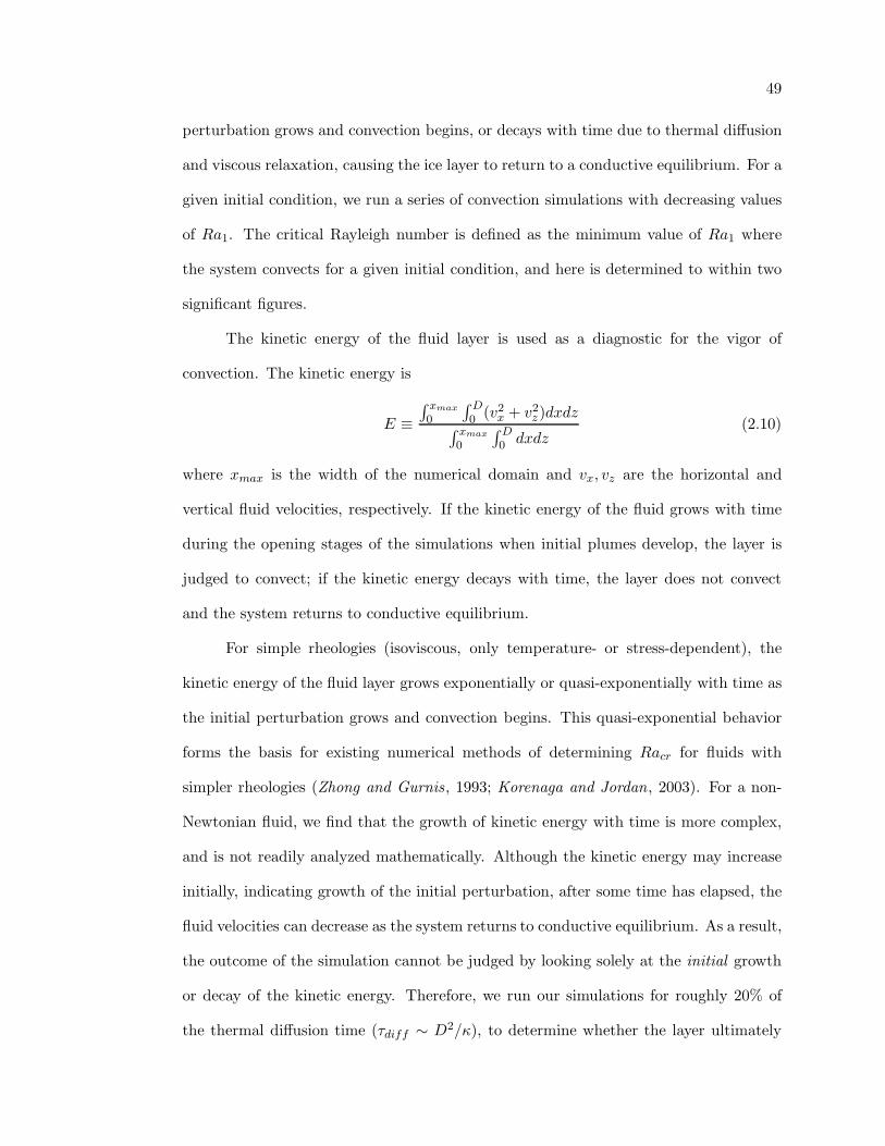
49

perturbation grows and convection begins, or decays with time due to thermal diffusion

and viscous relaxation, causing the ice layer to return to a conductive equilibrium. For a

given initial condition, we run a series of convection simulations with decreasing values

of Ra1. The critical Rayleigh number is defined as the minimum value of Ra1 where

the system convects for a given initial condition, and here is determined to within two

significant figures.

The kinetic energy of the fluid layer is used as a diagnostic for the vigor of

convection. The kinetic energy is

E ≡

∫ xmax

0

∫ D0 (v2

x + v2z)dxdz

∫ xmax

0

∫D0 dxdz

(2.10)

where xmax is the width of the numerical domain and vx, vz are the horizontal and

vertical fluid velocities, respectively. If the kinetic energy of the fluid grows with time

during the opening stages of the simulations when initial plumes develop, the layer is

judged to convect; if the kinetic energy decays with time, the layer does not convect

and the system returns to conductive equilibrium.

For simple rheologies (isoviscous, only temperature- or stress-dependent), the

kinetic energy of the fluid layer grows exponentially or quasi-exponentially with time as

the initial perturbation grows and convection begins. This quasi-exponential behavior

forms the basis for existing numerical methods of determining Racr for fluids with

simpler rheologies (Zhong and Gurnis, 1993; Korenaga and Jordan, 2003). For a non-

Newtonian fluid, we find that the growth of kinetic energy with time is more complex,

and is not readily analyzed mathematically. Although the kinetic energy may increase

initially, indicating growth of the initial perturbation, after some time has elapsed, the

fluid velocities can decrease as the system returns to conductive equilibrium. As a result,

the outcome of the simulation cannot be judged by looking solely at the initial growth

or decay of the kinetic energy. Therefore, we run our simulations for roughly 20% of

the thermal diffusion time (τdiff ∼ D2/κ), to determine whether the layer ultimately

50

returns to a conductive equilibrium or convects. The key advantage of this procedure is

that the final outcomes of our simulations are clearly self-sustaining convective states,

and not transient, quasi-stable states that convect briefly and return to conductive

equilibrium at a later time. The temperature field, velocity vectors, and viscosity fields

for a sample simulation where Ra = Racr for the basal slip rheology is shown in Figure

2.1. A sample graph of the evolution of kinetic energy over time is shown in Figure 2.2.

2.4 Model Results

2.4.1 Critical Rayleigh Number

The viscous restoring force that counteracts the buoyancy of a growing plume is

wavelength-dependent, so the critical Rayleigh number for convection will depend on

the wavelength of the perturbation, regardless of the rheology of the fluid. The critical

values of Rayleigh number (Racr) reported here are critical values of Ra1. We first

determine the wavelength that minimizes the value of Racr, then investigate how Racr

for that specific Fourier mode with λ = λcr varies with δT .

We find two regimes of behavior of the non-Newtonian ice shell. For small tem-

perature perturbations less than the rheological temperature scale (∆Trh), the critical

Rayleigh number depends on the amplitude of perturbation to a power θ. This is desig-

nated the power-law regime. For temperature perturbations greater than the rheological

temperature scale, the critical Rayleigh number approaches a constant value and is in-

dependent of the perturbation amplitude. This is designated the asymptotic regime.

The transition between the two regimes of behavior occurs when δT > ∆Trh,

∆Trh =1.2(n + 1)RT 2

i

Q∗, (2.11)

where Ti is the roughly constant temperature in the convective interior (Solomatov

and Moresi , 2000). Approximating Ti ∼ Tm, the rheological temperature scale is ap-

proximately 37 K for both rheologies, which corresponds to perturbation amplitudes of

51

-40

-30

-20

-10

0

Dep

th (

km)

0 10 20 30

X (km)

-40

-30

-20

-10

0

Dep

th (

km)

0 10 20 30

X (km)0 10 20 30

X (km)0 10 20 30

X (km)

-40

-30

-20

-10

0

Dep

th (

km)

0 10 20 30

X (km)

120 140160 180200 220 240260

T (K)

0 20 0 10 20 30

X (km)0 10 20 30

X (km)

14 15 16 17 18 19 20 21 22 23

log10η (Pa s)

a) t=0 b) t=0

c) t=5.8 Myr d) t=5.8 Myr

Figure 2.1: Temperature field (panel a) with superimposed velocity vectors, and vis-cosity field (panel b) with superimposed contours of constant viscosity for a sampleinitial condition from our study. The simulation is started with an initial temperatureperturbation of 15 K, and Ra = Racr = 4.0 × 104. This corresponds to an ice shell 49km thick on Ganymede with a surface temperature of 110 K, a melting temperature ofice of 260 K, and a grain size of ice of 1.0 mm. The initial condition evolves over 5.8Myr to generate the temperature and viscosity fields in panels c and d.

52

10-2

10-110-1

100

101

102

0.00 0.05 0.10 0.15 0.20

t’

EEEEEEConvection

No Convection

Figure 2.2: Growth of kinetic energy (E) with non-dimensional time (t’=t/τdiff ) for icewith GBS rheology with Ts = 110 K and Tm = 260 K, given an initial perturbation ofamplitude 0.75 K. Each line represents the evolution of kinetic energy for a simulationwith a different Rayleigh number from Ra1 = 1.8 × 105 (top line) to Ra1 = 1.3 × 105

(bottom line). After an initial phase of quasi-exponential growth of kinetic energy (fort′ < 0.05), the kinetic energy grows super-exponentially as convection begins. Wherekinetic energy does not grow, convection did not initiate. The highest Rayleigh numberthat resulted in convection, 1.6 × 105, is the critical Rayleigh number for this rheologyand set of boundary temperatures.

53

0.22∆T to 0.25∆T for the range of boundary temperatures considered here.

For a nominal set of boundary temperatures Ts = 110 K and Tm = 260 K, the

wavelength that minimizes Racr for both GBS and basal slip rheologies in the power law

regime is ∼ 1.5D, which does not change with the amplitude of perturbation. Figure

2.3 shows how Racr varies with wavelength for both rheologies, for the nominal set of

boundary temperatures. These values are substantially lower than λcr for an isoviscous

fluid (Turcotte and Schubert , 1982). This is likely because in a fluid with strongly

temperature-dependent rheology, initial fluid motions are confined to the bottom ∼30%

of the shell, decreasing the effective aspect ratio of the convecting region. The critical

Rayleigh number for the GBS and basal slip rheologies varies by a factor of two between

the minimum value when λ = λcr and the maximum value of wavelength used, λ = 3D.

In the asymptotic regime, 1.8D < λcr < 2.2D, and the critical Rayleigh number is very

weakly dependent on wavelength, varying by only 20% as λ is increased from 1.2D to

2.2D.

As discussed in section 2.3.1, the non-Newtonian deformation mechanisms begin

to control the growth of a perturbation at the base of the ice shell when the thermal

stress associated with the plume (σth ∼ ρgαδTλ) exceeds ∼ 0.02 MPa in ice with a

nominal grain size of 1.0 mm. For the average maximum permitted ice shell thickness

in Ganymede and Callisto of 170 km, a perturbation of 0.75 K above the ambient

conductive equilibrium spread across a horizontal distance ∼ D can generate ∼ 0.02

MPa, sufficient to activate grain boundary sliding and basal slip in ice with a grain size

of order 1 mm. In a relatively thin ice shell with D ∼ 20 km, a perturbation of ∼ 15

K is required to activate the non-Newtonian deformation mechanisms. These values

supply the minimum and maximum perturbation amplitude δT that we use, 0.005∆T

and 0.1∆T .

In the power law regime, the critical Rayleigh number varies as a power of the

54

0

25000

50000

75000

100000

Ra 1

1.0 1.5 2.0 2.5 3.0 3.5 4.0

Wavelength (λ/D)

0

25000

50000

75000

100000

Ra 1

1.0 1.5 2.0 2.5 3.0 3.5 4.0

Wavelength (λ/D)

0

25000

50000

75000

100000

Ra 1

1.0 1.5 2.0 2.5 3.0 3.5 4.0

Wavelength (λ/D)

0

25000

50000

75000

100000

Ra 1

1.0 1.5 2.0 2.5 3.0 3.5 4.0

Wavelength (λ/D)

GBS

Basal Slip

Figure 2.3: Critical Rayleigh number as a function of dimensionless wavelength forbasal slip rheology (diamonds) and grain boundary sliding rheology (GBS, dots) withTs = 110 K and Tm = 260 K. A constant perturbation amplitude of δT = 7.5 K is usedhere.

55

Table 2.1: Variation in Critical Rayleigh Number with Perturbation Amplitude

Rheology δT/∆T Racr

Basal Slip 0.005 1.2 × 105

0.010 8.0 × 104

0.025 4.6 × 104

0.050 3.1 × 104

0.075 2.4 × 104

0.100 2.0 × 104

Grain Boundary Sliding 0.005 1.6 × 105

0.010 1.2 × 105

0.025 7.7 × 104

0.050 5.5 × 104

0.075 4.6 × 104

0.100 4.0 × 104

amplitude of initial perturbation, obeying a relationship of form

Racr = Racr,0

(δT

∆T

)−θ

(2.12)

where Racr,0 and θ are determined with a least-squares fit to values of Racr in log-log

space. Figure 2.4 shows a sample set of Racr data for Ts = 110 K and Tm = 260 K for

both the GBS and basal slip rheologies, with values used in the plot listed in Table 2.1.

Figure 2.5 shows values of Racr in the power law and asymptotic regimes for basal slip

rheology with Ts = 110 K and Tm = 260 K.

Regardless of the boundary temperatures, the critical value of Ra1 varies by

approximately an order of magnitude over the range of δT explored. The onset of

convection is governed largely by the viscosity structure near the base of the ice shell,

which is controlled by the rheological temperature scale (Davaille and Jaupart , 1994):

∆Tη =−η(Tm)

∂η∂T

∣∣∣Tm

. (2.13)

For the form of rheology used here, the rheological temperature scale is given by

∆Tη =nRT 2

m

Q∗∆T, (2.14)

56

104

105105

Ra 1

1 2 5 10 20δT (K)

104

105105

Ra 1

1 2 5 10 20δT (K)

104

105105

Ra 1

1 2 5 10 20δT (K)

104

105105

Ra 1

1 2 5 10 20δT (K)

GBS

Basal Slip

Figure 2.4: Critical Rayleigh number as a function of the amplitude of initial tem-perature perturbation (δT ) for GBS (dots) and basal slip (diamonds) rheologies withTs = 110 K and Tm = 260 K. Lines are least squares fits to the data, where the sloperepresents the fitting coefficient θ in equation (2.12). For GBS, θ = 0.6, for basal slip,θ = 0.5.

57

104

105105

Ra 1

11 10 100δT (K)

104

105105

Ra 1

11 10 100δT (K)

Power Law

Asymptotic

Figure 2.5: Critical Rayleigh number as a function of the amplitude of initial tempera-ture perturbation (δT ) for basal slip rheology with Ts = 110 K and Tm = 260 K. In thepower law regime, for perturbation amplitudes less than ∼ 37 K, the critical Rayleighnumber is a function of perturbation amplitude. For perturbation amplitudes largerthan ∼ 37 K, the critical Rayleigh number reaches a constant value of 1.2 × 104.

58

and can be used to scale Racr,0 using:

Racr,0 = Ra0,0 + M∆Tη (2.15)

where M and Ra0,0 are the derived fitting coefficients.

In the asymptotic regime, the critical Rayleigh number does not depend on the

amplitude of temperature perturbation, and approaches an asymptotic value Raa. Val-

ues of Raa using λcr = 2.0D and δT = 0.35∆T are listed in Table 2.3.

Given a set of boundary temperatures, and amplitude of temperature pertur-

bation, the critical Rayleigh number in the power law regime can be estimated by

combining equations (2.12), (2.14), and (2.15):

Racr =

[

Ra0,0 + M

(nRT 2

m

Q∗∆T

)](δT

∆T

)−θ

. (2.16)

Values of the fitting coefficients Ra0,0, θ and M for both grain boundary sliding and basal

slip rheologies are shown in Table 2.2. We report Ra0,0 and M values for Tm = 260 K

only, and briefly discuss the effects of varying the melting temperature in section 2.4.3.

The expression for Racr in the power law regime is likely only valid when the ice

shell is in the stagnant lid convection regime, where viscosity contrast across the layer

is large and convective instability is limited to the warm, low-viscosity sub-layer near

the base of the ice shell. For the ice shell to be in the stagnant lid regime, the viscosity

contrast due to temperature alone, ∆ηT = (η(Ts)/η(Tm)) exceeds exp(4(n + 1)), or

7×104 for GBS and 8×105 for basal slip (Solomatov , 1995). For the range of boundary

temperatures used here, ∆ηT ranges from 2 × 106 to 2 × 1010 for GBS and 7 × 105 to

3 × 109 for basal slip.

59

Table 2.2: Numerically Determined Fitting Coefficients for Racr

Rheology Ra0,0 θ M

Grain Boundary Sliding 5.1 × 104 0.6 −2.7 × 105

Basal Slip 1.7 × 104 0.5 −7.7 × 104

2.4.2 Critical Shell Thickness

The critical shell thickness for the onset of convection due to small temperature

perturbations δT < ∆Trh can be obtained using the definition of Ra1:

Dcr =

(

Racr

(κdpA−1

)1/nexp

( Q∗

nRTm

)

ρgα∆T

)n/(n+2)

, (2.17)

where the value of Racr can be estimated using equation (2.16). The values of critical

Rayleigh number in the asymptotic regime can be used to determine an absolute lower

limit on the ice shell thickness required for convection. The lower limit on shell thickness

is obtained from Raa using:

Da =

(

Raa

(κdpA−1

)1/nexp

( Q∗

nRTm

)

ρgα∆T

)n/(n+2)

. (2.18)

In the power law regime, the critical grain size required to initiate convection in an ice

layer with thickness D is

dcrit =

(ρgαD(n+2)/n

(κA−1

)1/nexp

( Q∗

nRTm

)Racr

)n/p

. (2.19)

For d < dcr, convection can occur; for d > dcr the ice is too stiff to convect for the

given initial condition. The asymptotic value of Rayleigh number can also be used to

determine an upper limit on the grain size that can permit convection in a layer of

thickness D:

da =

(ρgαD(n+2)/n

(κA−1

)1/nexp

( Q∗

nRTm

)Raa

)n/p

. (2.20)

2.4.3 Variation of Melting Temperature

Two sets of simulations were run to quantify how much the critical Rayleigh

number is influenced by changing the melting temperature. In the case of GBS, Ts = 110

60

K and Tm = 270 K were used to obtain a relationship between δT and Racr. The

resulting values of Racr,0 and θ were compared to the values obtained when Tm = 260

K. For basal slip, procedure was repeated, using Tm = 250 K. In both cases, the fitting

coefficients obtained were different from their Tm = 260 K counterparts by only 1%. Use

of equation (2.16) for alternative melting temperatures between 250 K and 270 K is valid

for Racr to two significant figures, provided the high temperature creep enhancement

in ice near its melting point is not included in the rheology.

2.5 Comparison to Existing Studies

For simple rheologies, the critical Rayleigh number for convection in a fluid can be

obtained using linear stability anaylsis (Turcotte and Schubert , 1982; Chandrasekhar ,

1961). However, the critical Rayleigh number for the onset of convection in a non-

Newtonian fluid cannot be determined using linear stability analysis (Tien et al., 1969;

Solomatov , 1995). The viscosity of a non-Newtonian fluid depends on both temperature

and strain rate, so the viscosity in the perturbed layer of fluid depends on the amplitude

of the initial perturbation and becomes infinite as the amplitude of perturbation becomes

small (Solomatov , 1995). Convection in a non-Newtonian fluid with a temperature- and

strain-rate-depdendent rheology is always a finite-amplitude instability, and cannot be

readily analyzed analytically (Solomatov , 1995).

Analysis of the onset of convection in a fluid with stress-dependent (but not

temperature-dependent) rheology can provide constraints on how the non-Newtonian

behavior affects Racr. An alternative method of determining Racr for a non-Newtonian

fluid stems from a physical argument put forth by Chandrasekhar (1961), who pos-

tulated that the critical Rayleigh number occured at a critical temperature gradient

where the dissipation of energy by viscous forces in the system exactly balanced the

release of energy from the rising, thermally buoyant plume. Using an energy balance

argument, Tien et al. (1969) were able to calculate the critical Rayleigh number for

61

non-Newtonian fluids with a range of values of stress exponent, which compared fa-

vorably to their laboratory measurements of critical Rayleigh number for fluids with

stress-dependent rheologies.

The most widely-used results for the critical Rayleigh number for convection in a

non-Newtonian fluid arise from the pivotal study of Solomatov (1995), who built upon

the analysis of Tien et al. (1969) plus additional studies by Ozoe and Churchill (1972)

to consider a stress- and temperature-dependent rheology. With the knowledge that

the critical Rayleigh number for a non-Newtonian fluid depends on initial conditions,

Solomatov (1995) characterized the value of Rayleigh number where convection could

not occur, regardless of initial conditions.

The analysis of Solomatov (1995) focused on the behavior of the bottom thermal

boundary layer at the onset of convection. If the viscosity of the fluid depends strongly

on temperature, there are no fluid motions in the upper part of the convecting layer,

forming a stagnant lid. In the stagnant lid regime, convective motions are confined to

a warm sub-layer of the ice shell, where the temperature dependence of viscosity can

be neglected by evaluating the viscosity of the material at the mean temperature in the

sub-layer.

With this approximation, the critical Rayleigh number of the sub-layer can be

evaluated by assuming that the viscosity of ice depends only on stress, thus using the

results of Tien et al. (1969) and Ozoe and Churchill (1972). Convection in the entire

layer initiates when the local Rayleigh number of the bottom thermal boundary layer

exceeds a critical value. The critical Rayleigh number for entire fluid layer can therefore

be related to the critical Rayleigh number of the sub-layer.

To closely follow the analysis of Solomatov (1995), we non-dimensionalize our

rheology (equation 2.8) as

η′(T ′, ε′) = C1/nε′(1−n)/n exp

(

E

T ′ + T ′o

−E

1 + T ′o

)

(2.21)

62

Table 2.3: Comparison to Analysis of Solomatov (1995)

Rheology Ts (K) Raa (our study) Racr (Solomatov (1995))

Grain Boundary Sliding 90 3.1 × 104 2.3 × 104

100 2.7 × 104 1.9 × 104

110 2.2 × 104 1.5 × 104

120 1.9 × 104 1.2 × 104

Basal Slip 90 1.4 × 104 8.4 × 103

100 1.2 × 104 7.1 × 103

110 9.8 × 103 5.9 × 103

120 8.6 × 103 4.8 × 103

where C represents the pre-exponential parameters in the laboratory-derived flow law,

E = Q∗/(nR∆T ) is the non-dimensional activation energy, and T ′o = Ts/∆T is the

non-dimensional reference temperature.

The Rayleigh number of the unstable sub-layer of thickness zsub at the base of

the fluid layer is given by Solomatov (1995) as:

Rasub =ρgα∆Tz

2(n+1)/nsub

D(κC)1/n

exp

(E

1 + T ′o

−E

(1 − (zsub/2) + T ′o

)

(2.22)

where the viscosity is evaluated at the mean temperature in the sub-layer, T ′ = 1 −

(zsub/2), and the strain rate has been evaluated at κ/z2sub, the characteristic strain rate

in the sub-layer. The sub-layer reaches its maximum thickness and becomes convectively

unstable when the local Rayleigh number in the sub-layer is equal to the critical Rayleigh

number for a fluid with stress-dependent rheology:

Rasub(zmax) = Racr(n). (2.23)

The results of Tien et al. (1969) and Ozoe and Churchill (1972) are summarized and

extrapolated by Solomatov (1995) to obtain an approximation for the critical Rayleigh

number of a fluid with an arbitrary stress exponent:

Racr(n) ∼ Racr(1)1/nRacr(∞)(n−1)/n (2.24)

63

with Racr(1) = 1568, and Racr(∞) ∼ 20 represents the formal asymptotic limit of

Racr(n) for n → ∞.

The maximum sub-layer thickness (zmax) is obtained by solving for the value of

zsub that yields ∂Rasub/∂zsub = 0. For the form of temperature dependence used here,

we obtain a quadratic equation for zmax as a function of the non-dimensional activation

energy, stress exponent, and reference temperature. The quadratic equation yields two

results, but only the negative root yields physically applicable solutions where zsub < D:

zmax =D

2(n + 1)

(4(n + 1)(T ′

o + 1) + En − (8En(n + 1)(T ′o + 1) + E2n2)

)1/2. (2.25)

Substituting this value of zmax into equation (2.22) we obtain

Rasub =ρgα∆TD(n+2)/n

(κC)1/n

(zmax

D

)2(n+1)/n

exp

(E

1 + T ′o

−E

1 − zmax

2D + T ′o

)

. (2.26)

When using the non-dimensional rheology of form eq. (2.21), the viscosity at the melting

point and reference strain rate is equal to C1/n. Therefore, the first term in the above

equation is simply the critical Rayleigh number of the entire fluid layer, with η(Tm, εo).

Setting the expression for Rasub = Rasub(zmax) and solving for Racr we obtain:

Racr = Racr(n)

(zmax

D

)−2(n+1)/n

exp

(E

1 − zmax

2D + T ′o

−E

1 + T ′o

)

. (2.27)

Values of Racr from this analysis are compared to our numerically determined values of

critical Rayleigh number in the limit of the maximum permitted temperature pertur-

bation, δT → ∆Trh, Raa. The values of Raa from our study are summarized in Table

2.3. Agreement between our values of critical Rayleigh number and values obtained

using the method of Solomatov (1995) agree to within 35 to 60%. The variation in

Racr according to equation (2.27) is compared to numerically calculated values of Raa

in Figure 2.6.

64

0

10000

20000

30000

Ra c

r

80 90 100 110 120 130 140Ts (K)

0

10000

20000

30000

Ra c

r

80 90 100 110 120 130 140Ts (K)

0

10000

20000

30000

Ra c

r

80 90 100 110 120 130 140Ts (K)

GBS

Basal Slip

Figure 2.6: Comparison of our values of asymptotic critical Rayleigh number (Raa)calculated using λ = 2.0D and δT = 0.35∆T (dots=GBS, diamonds=basal slip) tocritical Rayleigh numbers calculated using the analysis of Solomatov (1995) (curves,bold=GBS, thin=basal slip), for various surface temperatures. Agreement between ourvalues and the analysis of Solomatov (1995) ranges from ∼ 35% to 60% as a functionof surface temperature.

65

2.6 Implications for the Icy Galilean Satellites

Gravity data do not place tight constraints on the thickness of the ice shells of any

of the icy Galilean satellites. The maximum thickness of Europa’s H2O layer is ∼ 170

km, but the fraction of the layer that is liquid is poorly constrained (Anderson et al.,

1998). The upper bounds on ice I shell thickness for all the icy satellites are obtained

by estimating the depth to the minimum melting point of ice I. The minimum melting

point occurs at a depth of approximately 170 km in Europa, 160 km in Ganymede, and

180 km in Callisto, if the density of the ice shell is 930 kg/m3 (Kirk and Stevenson,

1987; Ruiz , 2001). The grain sizes in the icy satellites are poorly constrained as well,

with estimates of grain size spanning eight orders of magnitude, from microns (Nimmo

and Manga, 2002) to meters (Schmidt and Dahl-Jensen, 2004). Conclusions regarding

the convective stability of the ice shells made here may not be correct if the grain sizes

in the satellites are much larger than 1 cm or smaller than 0.1 mm. Additionally, it is

plausible that the Goldsby and Kohlstedt (2001) rheology does not adequately describe

the true behavior of the ice shells of the Galilean satellites, for example, if impurities

have a significant effect on rheology. Moreover, we have ignored internal heating by

tidal dissipation in these calculations, a topic addressed in section 2.7.

If the high-temperature creep enhancement described in section 2.3.1 were in-

cluded in our models, the viscosities of ice at the base of the ice shell would be much

smaller, potentially permitting convection in significantly thinner ice shells. As the be-

havior of the convecting layer transitioned from initial plume growth to well-developed

convecting cells, the entire convecting sublayer of the ice shell could have a very low

viscosity due to the high-temperature softening. Because we have not included this

term, the critical ice shell thicknesses calculated using our models yield upper limits

on the shell thicknesses required for convection. More detailed calculations should be

performed in the future including this term in the rheology to investigate how high-

66

temperature softening of the ice affects both the onset of convection and the pattern of

convection.

In the likely event that the lab-derived flow law does not perfectly match the

true behavior of ice in the Galilean satellites, and that tidal dissipation plays a role in

modifying the thermal structure of the ice shells during the onset of convection, future

modeling efforts can use methods similar to those discussed here, to investigate more

thoroughly the conditions required to trigger convection in ice I shells.

2.6.1 Conditions for Convection in Callisto and Ganymede

Figure 2.7 shows the critical layer thickness for the onset of convection in Callisto’s

ice I shell for both grain boundary sliding and basal slip rheologies, if the ice has a grain

size of 1.0 mm. Similarly, Figure 2.8 shows the critical shell thickness on Ganymede.

For GBS, if the ice has a grain size of 1.0 mm, the critical shell thickness for convection

in Callisto’s ice shell varies between 103 km and the maximum permitted shell thickness

of 180 km for grain boundary sliding, and 32 km and 80 km for basal slip. In Ganymede,

if the ice has a grain size of 1.0 mm, the critical shell thickness ranges from 96 km to

greater than the maximum allowed ice shell thickness of 160 km, depending on surface

temperature. If flow is controlled by basal slip (which seems unlikely because the rate-

limiting flow law in the GSS deformation mechanism is GBS), the critical shell thickness

in Ganymede ranges from 30 km to 74 km.

In the more likely case that GBS is the controlling rheology, the largest initial

perturbation in this study (0.1∆T ) cannot trigger convection in either Ganymede or

Callisto’s ice shells with the nominal boundary temperatures if the ice near the base

of the ice shell has a grain size d > 3 mm (Figures 2.9 and 2.10). If the ice in either

satellite has a smaller grain size, convection can occur provided the requirements on shell

thickness and temperature perturbation are met. For GBS in an ice shell with a d = 1.0

mm and Ts = 110 K, a 5 K temperature perturbation can trigger convection in an ice

67

020406080

100120140160180200220

Dcr

(km

)

0 5 10 15δT (K)

020406080

100120140160180200220

Dcr

(km

)

0 5 10 15δT (K)

020406080

100120140160180200220

Dcr

(km

)

0 5 10 15δT (K)

020406080

100120140160180200220

Dcr

(km

)

0 5 10 15δT (K)

020406080

100120140160180200220

Dcr

(km

)

0 5 10 15δT (K)

020406080

100120140160180200220

Dcr

(km

)

0 5 10 15δT (K)

020406080

100120140160180200220

Dcr

(km

)

0 5 10 15δT (K)

020406080

100120140160180200220

Dcr

(km

)

0 5 10 15δT (K)

020406080

100120140160180200220

Dcr

(km

)

0 5 10 15δT (K)

DmaxDmax

020406080

100120140160180200220

Dcr

(km

)

0 5 10 15δT (K)

020406080

100120140160180200220

Dcr

(km

)

0 5 10 15δT (K)

020406080

100120140160180200220

Dcr

(km

)

0 5 10 15δT (K)

020406080

100120140160180200220

Dcr

(km

)

0 5 10 15δT (K)

020406080

100120140160180200220

Dcr

(km

)

0 5 10 15δT (K)

020406080

100120140160180200220

Dcr

(km

)

0 5 10 15δT (K)

90 K100 K

110 K120 K

Figure 2.7: Critical ice shell thicknesses (eq. 2.17) for the onset of convection in Callisto’sice shell, with grain boundary sliding (bold curves) or basal slip (thin curves) rheologies,for various surface temperature values. A constant grain size of 1.0 mm for the ice shellsis assumed for GBS, and a constant melting temperature of 260 K is assumed for bothrheologies. The maximum permitted ice shell thickness on Callisto, 180 km, is indicatedby the horizontal dashed line. The critical shell thickness predicted by the basal sliprheology ranges from 32 to 80 km over the range of δT considered.

68

020406080

100120140160180200

Dcr

(km

)

0 5 10 15δT (K)

020406080

100120140160180200

Dcr

(km

)

0 5 10 15δT (K)

020406080

100120140160180200

Dcr

(km

)

0 5 10 15δT (K)

020406080

100120140160180200

Dcr

(km

)

0 5 10 15δT (K)

020406080

100120140160180200

Dcr

(km

)

0 5 10 15δT (K)

020406080

100120140160180200

Dcr

(km

)

0 5 10 15δT (K)

020406080

100120140160180200

Dcr

(km

)

0 5 10 15δT (K)

020406080

100120140160180200

Dcr

(km

)

0 5 10 15δT (K)

020406080

100120140160180200

Dcr

(km

)

0 5 10 15δT (K)

DmaxDmax

020406080

100120140160180200

Dcr

(km

)

0 5 10 15δT (K)

020406080

100120140160180200

Dcr

(km

)

0 5 10 15δT (K)

020406080

100120140160180200

Dcr

(km

)

0 5 10 15δT (K)

020406080

100120140160180200

Dcr

(km

)

0 5 10 15δT (K)

020406080

100120140160180200

Dcr

(km

)

0 5 10 15δT (K)

020406080

100120140160180200

Dcr

(km

)

0 5 10 15δT (K)

90 K100 K

110 K120 K

Figure 2.8: Similar to Figure 2.7, but for Ganymede. Over the range of δT considered,the critical shell thickness ranges from 96 km to the maximum permitted shell thicknessof 160 km for GBS, which is the rate-limiting creep mechanism.

69

0.0010.001

0.01

0.1

1

d cr (

mm

)

0 30 60 90 120 150 180D (km)

0.0010.001

0.01

0.1

1

d cr (

mm

)

0 30 60 90 120 150 180D (km)

0.0010.001

0.01

0.1

1

d cr (

mm

)

0 30 60 90 120 150 180D (km)

0.0010.001

0.01

0.1

1

d cr (

mm

)

0 30 60 90 120 150 180D (km)

Convection

No Convection

0.0010.001

0.01

0.1

1

d cr (

mm

)

0 30 60 90 120 150 180D (km)

0.0010.001

0.01

0.1

1

d cr (

mm

)

0 30 60 90 120 150 180D (km)

0.0010.001

0.01

0.1

1

d cr (

mm

)

0 30 60 90 120 150 180D (km)

0.0010.001

0.01

0.1

1

d cr (

mm

)

0 30 60 90 120 150 180D (km)

0.0010.001

0.01

0.1

1

d cr (

mm

)

0 30 60 90 120 150 180D (km)

0.0010.001

0.01

0.1

1

d cr (

mm

)

0 30 60 90 120 150 180D (km)

90 K

100 K

110 K

120 K

Figure 2.9: Critical grain size for convection as a function of ice shell thickness (equation2.19) in Callisto’s ice shell with GBS rheology for various surface temperatures. Aconstant perturbation δT = 5 K is used here.

70

0.0010.001

0.01

0.1

1

d cr (

mm

)

0 30 60 90 120 150D (km)

0.0010.001

0.01

0.1

1

d cr (

mm

)

0 30 60 90 120 150D (km)

0.0010.001

0.01

0.1

1

d cr (

mm

)

0 30 60 90 120 150D (km)

0.0010.001

0.01

0.1

1

d cr (

mm

)

0 30 60 90 120 150D (km)

Convection

No Convection

0.0010.001

0.01

0.1

1

d cr (

mm

)

0 30 60 90 120 150D (km)

0.0010.001

0.01

0.1

1

d cr (

mm

)

0 30 60 90 120 150D (km)

0.0010.001

0.01

0.1

1

d cr (

mm

)

0 30 60 90 120 150D (km)

0.0010.001

0.01

0.1

1

d cr (

mm

)

0 30 60 90 120 150D (km)

0.0010.001

0.01

0.1

1

d cr (

mm

)

0 30 60 90 120 150D (km)

0.0010.001

0.01

0.1

1

d cr (

mm

)

0 30 60 90 120 150D (km)

90 K

100 K

110 K

120 K

Figure 2.10: Similar to Figure 2.9, but for Ganymede.

71

shell on Callisto ≥ 150 km thick. Under identical circumstances in Ganymede, Dcr is

141 km. The lower limit on ice shell thickness (Da) in the limit of large temperature

perturbations (in the asymptotic regime) varies from 50 to 57 km in Ganymede and 53

to 60 km in Callisto, as a function of surface temperature, if the ice has a grain size of

1.0 mm.

The equilibrium thicknesses for a conductive ice shell in Callisto and Ganymede

(in the absence of tidal dissipation) given the expected present-day radiogenic heating

rate of 4.5 × 10−12 W kg−1 (Spohn and Schubert , 2003), are 148 km, and 128 km

respectively. Triggering convection at present would require a temperature perturbation

of only 5 to 7 K, issued in the mathematical pattern described by equation (2.9) if λ =

λcr. If the perturbation is issued with a larger or shorter wavelength, the temperature

perturbation required to trigger convection will be larger.

Roughly 1.5 billion years ago when concentrations of 40K were higher, and radio-

genic heating rates were twice their present values, the equilibrium ice shell thicknesses

of Callisto and Ganymede would have been 74 km and 64 km, respectively. Triggering

convection in these ancient, thin ice shells of Callisto or Ganymede was only possible if

the grain size of ice was less than ∼ 2.5 mm, even if the amplitude of the temperature

perturbation was greater than ∆Trh. Therefore, initiating convection in an ice shell

may be easier later in the satellite’s history when decreased radiogenic heating allows

for a thicker ice shell.

2.6.2 Conditions for Convection in Europa

Figure 2.11 shows the critical layer thickness for convection in Europa’s ice shell,

with the simplifying assumption that the rapid tidal flexing of the shell does not affect

its rheology and merely results in tidal dissipation that perturbs the temperature field.

If the ice has a grain size of 1.0 mm, the critical shell thickness for the GBS rheology

ranges from 100 km to greater than the maximum permitted shell thickness of 170

72

020406080

100120140160180200220

Dcr

(km

)

0 5 10 15δT (K)

020406080

100120140160180200220

Dcr

(km

)

0 5 10 15δT (K)

020406080

100120140160180200220

Dcr

(km

)

0 5 10 15δT (K)

020406080

100120140160180200220

Dcr

(km

)

0 5 10 15δT (K)

020406080

100120140160180200220

Dcr

(km

)

0 5 10 15δT (K)

020406080

100120140160180200220

Dcr

(km

)

0 5 10 15δT (K)

020406080

100120140160180200220

Dcr

(km

)

0 5 10 15δT (K)

020406080

100120140160180200220

Dcr

(km

)

0 5 10 15δT (K)

020406080

100120140160180200220

Dcr

(km

)

0 5 10 15δT (K)

DmaxDmax

020406080

100120140160180200220

Dcr

(km

)

0 5 10 15δT (K)

020406080

100120140160180200220

Dcr

(km

)

0 5 10 15δT (K)

020406080

100120140160180200220

Dcr

(km

)

0 5 10 15δT (K)

020406080

100120140160180200220

Dcr

(km

)

0 5 10 15δT (K)

020406080

100120140160180200220

Dcr

(km

)

0 5 10 15δT (K)

020406080

100120140160180200220

Dcr

(km

)

0 5 10 15δT (K)

90 K100 K

110 K120 K

Figure 2.11: Similar to Figure 2.7, but for Europa. The critical ice shell thickness rangesfrom 100 km to the maximum permitted shell thickness of 170 km for the GBS rheology,and from 31 to 78 km for basal slip.

73

km; for the basal slip rheology, the critical shell thickness ranges from and 31 km to

78 km. Triggering convection in an ice shell with the nominally accepted thickness

of 20-25 km (Pappalardo et al., 1999; Nimmo et al., 2003) with GBS rheology in the

asymptotic regime with a large temperature perturbation requires the ice has a grain

size ≤ 0.07 − 0.1 mm, respectively. Larger grain sizes lead to stiffer ice, and convection

is not permitted, even if δT ≫ ∆Trh. Figure 2.12 demonstrates that for the GBS

rheology, triggering convection with a temperature perturbation of amplitude 5 K in

the thickest possible ice shell in Europa requires a grain size ≤ 2.0 mm. This conclusion

regarding the grain size is qualitatively similar to the conclusions made by McKinnon

(1999), but consideration of the non-Newtonian rheology adds an additional constraint:

a temperature perturbation must be issued to the ice shell to soften the ice in order to

trigger convection.

2.7 Discussion: The Role of Tidal Dissipation

Tidal dissipation is a likely mechanism to generate temperature anomalies of

order 1-10’s K within the ice shells of tidally flexed satellites. Although estimates of

the total amount of dissipation within Ganymede and Europa exist, how this heat is

distributed within their ice shells is a poorly constrained problem. If tidal dissipation is

concentrated on spatial scales much longer than λcr, triggering convection with may not

be possible even in the thickest ice shells in Ganymede and Europa if ice flows by GBS

only. Tidal heating may concentrate in zones of weakness in the ice shell, providing a

laterally heterogeneous heat source within the ice shell [e.g. Tobie et al., 2004]. Zones

of weakness could form beneath double ridges on Europa, whose upwarped morphology

may be due to thermal and/or compositional buoyancy driven by localized shear heating

generated by cyclical lateral motion along strike-slip faults (Nimmo and Gaidos, 2002).

If the tidal dissipation is concentrated within the ice shells on spatial scales similar to

λcr, convection could be triggered by tidal heating in shells thinner than the maximum

74

0.0010.001

0.01

0.1

1

d cr (

mm

)

0 30 60 90 120 150D (km)

0.0010.001

0.01

0.1

1

d cr (

mm

)

0 30 60 90 120 150D (km)

0.0010.001

0.01

0.1

1

d cr (

mm

)

0 30 60 90 120 150D (km)

0.0010.001

0.01

0.1

1

d cr (

mm

)

0 30 60 90 120 150D (km)

Convection

No Convection

0.0010.001

0.01

0.1

1

d cr (

mm

)

0 30 60 90 120 150D (km)

0.0010.001

0.01

0.1

1

d cr (

mm

)

0 30 60 90 120 150D (km)

0.0010.001

0.01

0.1

1

d cr (

mm

)

0 30 60 90 120 150D (km)

0.0010.001

0.01

0.1

1

d cr (

mm

)

0 30 60 90 120 150D (km)

0.0010.001

0.01

0.1

1

d cr (

mm

)

0 30 60 90 120 150D (km)

0.0010.001

0.01

0.1

1

d cr (

mm

)

0 30 60 90 120 150D (km)

90 K

100 K

110 K

120 K

Figure 2.12: Similar to Figure 2.9, but for Europa.

75

allowed shell thickness of 160 km in Ganymede and 170 km in Europa.

Tidal dissipation may change the mode of heat transfer across the outer ice I

shells of tidally flexed icy satellites such as Ganymede or Europa during past epochs

of increased tidal activity (Showman and Malhotra, 1997; Hussmann and Spohn, 2004).

We envision two possible scenarios. If the ice shell is initially in conductive equilibrium

when tidal dissipation begins, dissipation would be concentrated where the viscosity of

the ice is such that the tidal forcing time scale is equal to the Maxwell time of the ice,

likely at the warm base of the shell (Ojakangas and Stevenson, 1989). This addition

of heat would raise the local temperature above the conductive equilibrium, potentially

causing the bottom layer of the ice shell to become convectively unstable. Conversely,

if the ice shell is initially convecting when tidal dissipation begins and the heat flux

due to tidal dissipation exceeds the convective heat flux, the ice shell would thin by

melting, and convection would cease McKinnon (1999), and convection would be only

a transient phenomenon occurring only in the beginning stages of passage through an

orbital resonance. The existence of an equilibrium between tidal dissipation and the

convective heat flux is controlled by the actual rheology of the ice shell and the details

of tidal dissipation, both of which are not well constrained.

Given the requirement of a finite-amplitude temperature perturbation to initiate

convection in a non-Newtonian ice shells, tidal dissipation could be required to initiate

convection in all icy satellites. A causal relationship between tidal dissipation and

endogenic resurfacing is supported by the observation that all endogenically-resurfaced

icy satellites in the solar system are presently in or have passed through, an orbital

resonance (Dermott et al., 1988; Showman and Malhotra, 1997; Goldreich et al., 1989).

If this is the case, the endogenic resurfacing on Europa and Ganymede could have

been formed during a brief transient period during which tidal dissipation occurred,

triggering convection. Because Callisto has apparently not undergone tidal dissipation,

its non-Newtonian outer ice I shell may have never convected, and therefore has never

76

experienced endogenic resurfacing.

2.8 Summary

The laboratory-derived composite flow law for ice I implies that the growth of

modest-amplitude (∼ 1-10’s K) temperature perturbations in an ice shell is governed

by non-Newtonian creep mechanisms. Therefore, the initiation of convection depends

on the success of plume growth under the influence of these non-Newtonian deforma-

tion mechanisms, which place stringent requirements on the thickness and grain size of

an ice I shell. In the absence of tidal dissipation, the initiation of convection depends

on growth of temperature perturbations governed by the non-Newtonian rheology of

grain boundary sliding. For temperature perturbations larger than the rheological tem-

perature scale (> 37 K), the critical Rayleigh number is independent of perturbation

amplitude and yields an lower limit on the shell thickness required for convection if ice

deforms by GBS or basal slip only.

In Callisto, the critical shell thickness ranges between 103 km and the maximum

permitted shell thickness of 180 km. In Ganymede, the critical ice shell thickness for

convection controlled by GBS in ice with a nominal grain size of 1.0 mm is between

96 km and the maximum permitted ice I shell thickness of 160 km. In both satellites,

convection can only be triggered by modest temperature perturbations of 1-10’s K if

the grain size is less than 1.0 mm. If larger temperature perturbations are issued to the

ice shell by, for example, tidal dissipation, convection may occur in ice shells with larger

grain sizes.

In Europa, the critical shell thickness for convection ranges from 100 to the max-

imum permitted shell thickness of 170 km, for GBS and a grain size of 1.0 mm. Con-

vection in a Europan ice shell thicker than 100 km can be initiated from modest 1-10’s

K temperature perturbations if the grain size of ice is small, less than 2.0 mm.

Extrapolations of these results to other icy satellites, boundary temperatures,

77

grain sizes, and rheologies can be made using the derived relationships among the phys-

ical, thermal, and rheological parameters of the system and the critical Rayleigh num-

ber. Convection can be initiated from a conductive equilibrium in the non-Newtonian

ice shells of Europa, Ganymede, and Callisto if a temperature perturbation is issued to

the ice shell to soften the ice and permit fluid motion. The critical Rayleigh number and

conditions permitting convection depend on the amplitude and wavelength of tempera-

ture perturbation issued to the ice shell. For the Galilean satellites, large temperature

perturbations of order 10’s K are required to initiate convection in ice shells thinner

than 100 km, regardless of grain size. For perturbation amplitudes greater than 37 K,

the critical Rayleigh number is constant, indicating that regardless of the amplitude of

perturbation, convection may not be possible in ice shells with large grain size. Re-

gardless of the critical ice shell thickness required for convection, the non-Newtonian

behavior of ice requires that a finite-amplitude temperature perturbation be issued to

the shell to trigger convection. Tidal dissipation may be required to generate initial

temperature perturbations, suggesting that convection may only occur in thin outer ice

I shells of satellites when the shell is tidally flexed.

Chapter 3

Onset of Convection in Ice I with Composite Newtonian and

Non-Newtonian Rheology

This chapter has been submitted to the Journal of Geophysical Research:

Barr, A. C. and R. T. Pappalardo (2004), Onset of Convection in Ice I with

Composite Newtonian and non-Newtonian Rheology: Application to the Icy Galilean

Satellites J. Gephys. Res., 2004JE002371, submitted.

3.1 Abstract

Ice I exhibits a complex rheology at temperature and pressure conditions appro-

priate for the interiors of the outer ice shells of Europa, Ganymede, and Callisto. We

use numerical methods to determine the conditions required to trigger convection in

an ice I shell with the stress-, temperature- and grain size-dependent composite rheol-

ogy measured in laboratory experiments by Goldsby and Kohlstedt (2001). The critical

Rayleigh number for convection varies as a power (−0.2) of the amplitude of initial tem-

perature perturbation, for perturbation amplitudes between 3 K and 30 K. The critical

Rayleigh number depends strongly on the grain size of ice, which governs the transi-

tion stresses between the Newtonian and non-Newtonian deformation mechanisms. The

critical ice shell thickness for convection in all three satellites is < 30 km if the ice

grain size is <1 mm. In this case, the relatively low thermal stresses associated with

plume growth are not sufficient to activate weakly non-Newtonian grain-size-sensitive

79

(GSS) creep, so plume growth is controlled by Newtonian volume diffusion. The critical

shell thickness is <30 km for grain sizes >1 cm, where thermal stresses can activate

strongly non-Newtonian dislocation creep, and the ice softens as it flows. For interme-

diate grain sizes (1-10 mm), weakly non-Newtonian grain-size-sensitive creep controls

plume growth, yielding critical shell thicknesses close to the maximum permitted shell

thickness for each of the Galilean satellites. Regardless of the rheology that controls

initial plume growth, a finite amplitude temperature perturbation is required to soften

the ice to permit convection, and this may require tidal dissipation.

3.2 Introduction

Chapter 2 examined the convective stability of an initially conductive ice I shell

under the influence of two of the weakly non-Newtonian deformation mechanisms in ice,

namely grain boundary sliding (GBS) and basal slip (bs). That work characterized the

critical Rayleigh number in two regimes of behavior. For modest amplitude temperature

perturbations, the critical Rayleigh number was found to be a function of the amplitude

of initial temperature perturbation. In the limit of large amplitude perturbations (> 37

K), the critical Rayleigh number was found to approach a constant, asymptotic value. In

the power law regime, the critical Rayleigh number for convection in ice with a rheology

of only GBS or only basal slip was found to vary by an order of magnitude as the

amplitude of initial temperature perturbation varies from 0.7 K to 17 K. In Chapter 2, we

concluded that convection could occur in the outer ice I layers of Europa, Ganymede, and

Callisto provided stringent requirements on shell thickness, perturbation amplitude, and

grain size are met simultaneously. If deformation in ice was accommodated by the GBS

deformation mechanism alone, then convection in Europa, Ganymede, or Callisto could

only occur in an ice shell with a grain size of 1 mm or less, triggered by a temperature

perturbation of order 1-10 K in shell greater than 100 km thick.

However, GBS and basal slip accommodate deformation in ice I only for a small

80

range of temperatures, grain sizes, and stresses, and the roles of the Newtonian deforma-

tion mechanism of diffusional flow and the highly non-Newtonian mechanism dislocation

creep were left unaddressed in Chapter 2. Using similar numerical methods, we extend

the results of this previous work to determine the conditions required to trigger con-

vection in an ice I shell using a composite Newtonian and non-Newtonian rheology for

ice.

3.3 Methods

3.3.1 Numerical Implementation of Composite Rheology for Ice I

Laboratory experiments indicate that deformation in ice I is accommodated by

four creep mechanisms, resulting in a composite flow law (Goldsby and Kohlstedt , 2001):


(

1

εbs+

1

εGBS

)−1

. (3.1)

The composite flow law includes contributions from diffusional flow (diff ), dislocation

creep (disl), and grain-size-sensitive creep (GSS), where deformation occurs by both

basal slip (bs) and grain boundary sliding (GBS ) (Goldsby and Kohlstedt , 2001). Basal

slip and GBS are dependent mechanisms and both must operate simultaneously to

permit deformation. When responsible for flow, the total strain rate for GSS is controlled

by the slower of the two constituent mechanisms (Durham and Stern, 2001).

The vertical viscosity structure near the base of the ice shell controls the viscous

restoring forces that retard growth of initial convective plumes, so estimates of the grain

size near the melting point of ice are useful for evaluating the conditions required to

permit convection. The grain sizes of ice in the satellites are not well constrained, with

estimates spanning eight orders of magnitude, from microns (Nimmo and Manga, 2002)

to meters (Schmidt and Dahl-Jensen, 2004). Terrestrial ice sheets under similar stress

and temperature conditions as the base of Europa’s ice shell exhibit grain sizes of order 1

mm (De La Chapelle et al., 1998). Grain growth in Europa’s ice shell would be limited

81

by rapid tidal flexing of the ice shell and by the presence of non-water-ice materials

(McKinnon, 1999). The presence of non-water-ice materials in the shells of Ganymede

and Callisto might similarly limit grain growth in these satellites as well.

To account for the uncertainty in the grain size of ice within the icy Galilean

satellites, we use grain sizes ranging from 0.1 mm to 10 cm. We characterize the

conditions required for convection as a function of grain size. We assume that the

ice shells have a uniform grain size, which is implausible in a real ice shell.

The strain rate for each creep mechanism in the composite rheology (equation

3.1) is described by

ε = Aσn

dpexp

(−Q∗

RT

)

, (3.2)


exponent, d is the ice grain size, p is the grain size exponent, Q∗ is the activation energy,

R is the gas constant, and T is temperature. Rheological parameters after Goldsby and

Kohlstedt (2001) are summarized in Table A.2.

Goldsby and Kohlstedt (2001) provide an alternate set of creep parameters for

GBS and dislocation creep for ice near its melting point. For T > 255 K, deformation

rates in ice due to GBS are increased by a factor of 1000, in response to melting at

grain boundaries and edges, resulting in very low viscosities near the melting point.

This behavior is consistent with observations of grain size, temperature, stress, and

strain rate for terrestrial ice cores (De La Chapelle et al., 1998). A similar effect occurs

for dislocation creep at T > 258 K. We have not included the high temperature creep

enhancement in our initial numerical models. Use of the creep enhancement for warm

ice alone will result in extremely low viscosities near the base of the ice shell, which

presents a difficulty for our numerical model.

The strain rate from diffusion creep is described by

ε =42Vmσ

RTmd2

(

Dv +πδ

dDb

)

(3.3)

82

where Vm is the molar volume, Tm is the melting temperature of ice, Dv is the rate of

volume diffusion, δ is the grain boundary width, and Db is the rate of grain boundary

diffusion (Goodman et al., 1981; Goldsby and Kohlstedt , 2001).

The grain sizes we consider are much larger than the grain boundary width

(9.04 × 10−10 m) (Goldsby and Kohlstedt , 2001), so volume diffusion dominates over

grain boundary diffusion, and we may ignore the contribution of grain boundary diffu-

sion to the strain rate. The strain rate for volume diffusion is:

εdiff =Adiff

d2Do,v exp

(−Q∗

v

RT

)

(3.4)

where Do,v is the volume diffusion rate coefficient and Qv is the activation energy. The

viscosity of ice deforming by volume diffusion is Newtonian, but it does depend on grain

size. The parameters for volume diffusion are listed in Table A.2, where we have grouped

the pre-exponential parameters to calculate an effective Adiff = (42VmDo,v/RTm).

The deformation mechanism that yields the highest strain rate for a given tem-

perature and differential stress is inferred to accommodate deformation in ice at that

temperature and stress level. The transition stress between any pair of flow laws, for

example, GBS and dislocation creep, is described by

σT =

[

AGBS

Adisl

dpdisl

dpGBSexp

((Q∗

disl − Q∗GBS)

RT

)]1

ndisl−nGBS

. (3.5)

The expressions for the transition stresses between the various deformation mechanisms

can be used to construct deformation maps showing the boundaries of regimes of domi-

nance for each constitutent creep mechanism. Deformation maps for ice with grain sizes

0.1 mm, 1.0 mm, 1.0 cm, and 10 cm are illustrated in Figure 3.1.

The strain from a growing convective plume will be accommodated by the de-

formation mechanism that is dominant near the melting temperature of ice and the

thermal stress exerted by the growing plume. The thermal stress due to a plume of

height λ, warmer than its surroundings by δT , is approximately σth ∼ ρgαδTλ. In an

83

-4

-2

0

2lo

g 10

σ (M

Pa)

120 150 180 210 240

-4

-2

0

2lo

g 10

σ (M

Pa)

120 150 180 210 240

-4

-2

0

2lo

g 10

σ (M

Pa)

120 150 180 210 240

-4

-2

0

2lo

g 10

σ (M

Pa)

120 150 180 210 240

Disl

GBS

d=10 cm

120 150 180 210 240

120 150 180 210 240

120 150 180 210 240

120 150 180 210 240

Disl

Diff

GBS

d=1.0 cm

-4

-2

0

2

log 1

0 σ

(M

Pa)

120 150 180 210 240T (K)

-4

-2

0

2

log 1

0 σ

(M

Pa)

120 150 180 210 240T (K)

-4

-2

0

2

log 1

0 σ

(M

Pa)

120 150 180 210 240T (K)

-4

-2

0

2

log 1

0 σ

(M

Pa)

120 150 180 210 240T (K)

Disl

GBS

BS Diff

d=1.0 mm

120 150 180 210 240T (K)

120 150 180 210 240T (K)

120 150 180 210 240T (K)

120 150 180 210 240T (K)

Disl

GBS

BS

Diff

d=0.1 mm

Figure 3.1: Deformation maps for ice I using the rheology of Goldsby and Kohlstedt(2001), for ice with grain sizes of 10 cm, 1.0 cm, 1.0 mm, and 0.1 mm. Lines on thedeformation maps represent the transition stress between mechanisms as a function oftemperature. A melting temperature of 260 K is assumed. For large grain sizes, dislo-cation creep (n=4) dominates the rheological behavior for thermal stresses associatedwith initial plume growth in the icy satellites (∼ 10−4 − 10−2 MPa). The weakly non-Newtonian deformation mechanisms play important roles for intermediate grain sizes(1.0 cm and 1.0 mm). Diffusional flow, which is a Newtonian deformation mechanism,becomes important at small stresses, small grain sizes, and temperatures close to themelting point.

84

ice shell 50 km thick on Europa, Ganymede, or Callisto, a plume with height λ ∼ D and

δT ∼ 5 K can generate a thermal stress of ∼0.03 MPa. In an ice shell 25 km thick, a

plume of height approximately 25 km can generate ∼0.15 MPa. For the range of grain

sizes considered, the thermal stresses associated with initial plume growth can activate

any of the four deformation mechanisms, with dislocation creep controlling initial plume

growth for grain sizes of 10 cm, and diffusional flow controlling plume growth in ice with

a grain size of 0.1 mm.

Each deformation mechanism in the composite rheology has a distinct stress ex-

ponent and activation energy, so inversion of equation (3.1) for an exact expression for

viscosity (η = σ/ε) is not possible. van den Berg et al. (1995) implement a compos-

ite rheology for mantle materials, including a term for Newtonian diffusional flow and

non-Newtonian dislocation creep. To derive an expression for the total viscosity due to

all four deformation mechanisms, we follow the procedure described by van den Berg

et al. (1995) by expressing the composite flow law (equation 3.1) in terms of viscosities

as η = σ/ε. This procedure yields an approximate solution for the effective viscosity

due to all four deformation mechanisms as

ηeff =

[

1

ηdiff+

1

ηdisl+

(

ηbs + ηGBS

)−1]−1

. (3.6)

This approximation provides a good estimate of the total viscosity for most values of

stress and temperature. This approximation underestimates the viscosity by a factor of

∼ 3 near the transition stresses between pairs of deformation mechanisms. Figure 3.2

illustrates a representative plot of viscosity as a function of stress for various grain sizes

at a temperature of 185 K.


An explicit stress-dependent rheology of form

η =dp

Aσ(1−n) exp

( Q∗

RT

)

(3.7)

85

10

15

20

25

log 1

0 η

(Pa

s)

-4 -2 0 2log10(σ (MPa))

10

15

20

25

log 1

0 η

(Pa

s)

-4 -2 0 2log10(σ (MPa))

10

15

20

25

log 1

0 η

(Pa

s)

-4 -2 0 2log10(σ (MPa))

10

15

20

25

log 1

0 η

(Pa

s)

-4 -2 0 2log10(σ (MPa))

10

15

20

25

log 1

0 η

(Pa

s)

-4 -2 0 2log10(σ (MPa))

10

15

20

25

log 1

0 η

(Pa

s)

-4 -2 0 2log10(σ (MPa))

10

15

20

25

log 1

0 η

(Pa

s)

-4 -2 0 2log10(σ (MPa))

10

15

20

25

log 1

0 η

(Pa

s)

-4 -2 0 2log10(σ (MPa))

10

15

20

25

log 1

0 η

(Pa

s)

-4 -2 0 2log10(σ (MPa))

10

15

20

25

log 1

0 η

(Pa

s)

-4 -2 0 2log10(σ (MPa))

10

15

20

25

log 1

0 η

(Pa

s)

-4 -2 0 2log10(σ (MPa))

10

15

20

25

log 1

0 η

(Pa

s)

-4 -2 0 2log10(σ (MPa))

10

15

20

25

log 1

0 η

(Pa

s)

-4 -2 0 2log10(σ (MPa))

10

15

20

25

log 1

0 η

(Pa

s)

-4 -2 0 2log10(σ (MPa))

10

15

20

25

log 1

0 η

(Pa

s)

-4 -2 0 2log10(σ (MPa))

10

15

20

25

log 1

0 η

(Pa

s)

-4 -2 0 2log10(σ (MPa))

10

15

20

25

log 1

0 η

(Pa

s)

-4 -2 0 2log10(σ (MPa))

Diff

10

15

20

25

log 1

0 η

(Pa

s)

-4 -2 0 2log10(σ (MPa))

GBS10

15

20

25

log 1

0 η

(Pa

s)

-4 -2 0 2log10(σ (MPa))

Basal Slip

10

15

20

25

log 1

0 η

(Pa

s)

-4 -2 0 2log10(σ (MPa))

Disl

d=10 cm

d=1 cm

d=1 mm

d=0.1 mm

Figure 3.2: Composite Newtonian/non-Newtonian viscosity for ice I as a function ofstress for grain sizes 10 cm, 1 cm, 1 mm, and 0.1 mm, and a constant temperatureof T = 185 K (black lines). The family of solid green lines indicates the viscosityfor diffusional flow, which is Newtonian and independent of stress, but dependent ongrain size. The family of dotted blue lines indicate the viscosity for GBS, which isweakly stress-dependent and grain size-dependent. Lines for dislocation creep (dot-dashed orange) and basal slip (dashed red) are shown as well. The composite viscosityis approximate near the transition stresses between flow laws, represented here whereany two viscosity curves cross.

86

is used for each term in equation (3.6). To phrase the rheology in non-dimensional

terms, we divide each term in the expression for total viscosity by the viscosity due to

diffusional flow at the melting temperature of ice,

ηo =RTmd2

42VmDo,vexp

( Q∗v

RTm

)

. (3.8)

We use a reference viscosity (ηo) defined by the viscosity due to volume diffusion at the

melting temperature of ice, which yields a reference Rayleigh number for the ice shell

given by

Rao =ρgα∆TD3

κηo, (3.9)

similar to the definitions used in Newtonian studies.

The definition of the reference Rayleigh number (Rao) is purely for algebraic con-

venience, so the values of the Rayleigh number used in simulations with large grain size

where the ice becomes strongly non-Newtonian may seem counterintuitive (for example,

Rao = 10−2). In a non-Newtonian fluid, as the fluid begins to flow and convection starts,

the viscosities in the fluid layer decrease, and the viscosity in the convecting sublayer

may be several orders of magnitude lower than ηo. A more physically intuitive definition

of Rayleigh number in the non-Newtonian case is the effective Rayleigh number:

Raeff =Raoηo

〈η〉, (3.10)

where the average viscosity in the convecting sublayer 〈η〉, which can be calculated after

the convection simulation is run to steady state. However, we do not run our simulations

to steady state, because we study the growth of initial convective plumes, so we cannot

calculate 〈η〉. Because we can not calculate Raeff , the viscosity near the warm base of

the ice shell can be used to provide some physical insight into the behavior of the ice

shell under the composite rheology. The viscosity at the melting point near the base of

the ice shell is 1013 Pa s when volume diffusion and dislocation creep are the dominant

rheologies. When GSS creep accommodates convective strain, the viscosity at the base

of the ice shell is 1015 to 1016 Pa s.

87

We represent the transition stresses between the various deformation mechanisms

in the expression for total viscosity (equation 3.6) by a series of relative weighting factors

between the four rheologies, which govern the relative importance of each deformation

mechanism as a function of temperature and grain size. The weighting factor for dislo-

cation creep, for example, is given by

βdisl =A

dpηn

o ε(n−1)o , (3.11)

where ηo is the reference viscosity, and εo is the reference strain rate. The weighting

factors for basal slip and GBS have a similar form. The viscosity due to diffusional

flow has a weighting factor of 1 at T = Tm, and for example, values of βdisl range

from 1020 for a grain size of 10 cm to 10−4 for a grain size of 0.1 mm. Values of β for

each viscosity function are summarized in Table B.7. Each viscosity function becomes

non-dimensionalized as:

η′ =1

βσ′(1−n) exp

( E

T ′ + T ′o

−Ev

1 + T ′o

)

(3.12)

where primed quantities are non-dimensionalized, σ′ = σ/(ηoεo) is non-dimensional

stress, E = (Q∗/nR∆T ) is the non-dimensional activation energy, Ev = Q∗v/nR∆T

is the non-dimensional activation energy for volume diffusion, and T ′o = Ts/∆T is the

reference temperature. In this formulation, the relative weights, transition stresses,

and reference viscosity depend strongly on the grain size of ice. Values of thermal and

physical parameters used in this study are summarized in Table A.1.

We have implemented the composite rheology for ice in the finite-element convec-

tion model Citcom (Moresi and Gurnis, 1996; Zhong et al., 1998, 2000), which solves

the governing equations of thermally driven convection in an incompressible fluid. Our

simulations are run in 2D Cartesian geometry. Free-slip boundary conditions are used

on the surface (z = 0), base (z = −D), and edges (x = 0, xmax) of the domain. All

simulations in this study were performed in a domain with 32 x 32 elements, chosen to

88

resolve the bottom thermal boundary layer while allowing sufficient coverage of our large

parameter space given limited computational resources. To ensure numerical stability,

an upper viscosity cutoff of 1010ηo was imposed.

The layer is purely basally heated, so internal heating by tidal dissipation is

not considered. However, tidal heating likely plays a role in triggering convection in

the icy satellites by generating finite-amplitude temperature perturbations to soften

the ice (see Chapter 2), and potentially by modifying the viscosity and grain size of

the ice shell (McKinnon, 1999), which we discuss in sections 3.5.3 and 3.5.4. The

surface of the convecting layer is held at a constant temperature of 110 K, approximately

average for the equatorial surfaces of the Jovian icy satellites. We also use a single

nominal value of melting temperature for ice, 260 K. In Chapter 2, variation of melting

temperature is shown to have a small effect on the values of critical Rayleigh number and

conditions for convection in the satellites. We have not taken into account the thermal

or rheological effects of contaminant non-water-ice materials such as hydrated sulfuric

acid, or hydrated sulfate salts, which have been suggested to exist on the surfaces of

the satellites based on near-infrared spectroscopy (McCord et al., 1999; Carlson et al.,

1999). We have also not included terms in the Goldsby and Kohlstedt (2001) rheology

for high temperature creep enhancement due to premelting in ice.

In the absence of benchmarking data with rheologies similar to those used here,

we perform two types of checks on the validity of our model. First, we compare the

results of simulations with a simple strain rate-dependent composite Newtonian and

non-Newtonian (n=3) rheology to the results of van den Berg et al. (1993). We find

good qualitative agreement between the published solutions and our results by matching

viscosity, velocity, and temperature fields, as well as time evolution of kinetic energy

and heat flux.

89


The approach we use to numerically determine the critical Rayleigh number is

similar to linear stability analysis (Turcotte and Schubert , 1982; Chandrasekhar , 1961).

The convection simulations are started from an initial condition of a conductive ice shell

plus a temperature perturbation expressed as a single Fourier mode:

T (x, z) = Ts −z∆T

D+ δT cos

(2πD

λx

)

sin

(−zπ

D

)

(3.13)

where δT and λ are the amplitude and wavelength of the temperature perturbation,

and z = −D at the warm base of the ice shell. Use of free-slip boundary conditions

requires that the width of the computational domain (xmax) be equal to one half the

wavelength of initial perturbation. The simulation is run for a short time to determine

whether the initial perturbation grows and convection begins, or decays with time due to

thermal diffusion and viscous relaxation, causing the ice layer to return to a conductive

equilibrium (Barr et al., 2004). For a given initial condition, we run a series of convection

simulations with decreasing values of Rao. The critical Rayleigh number is defined as

the minimum value of Rao where the system convects for a given initial condition, and

here is determined to three significant figures.

Based on results from Chapter 2, we expect the critical Rayleigh number to

depend on a power of the amplitude of the initial temperature perturbation for pertur-

bations smaller than the rheological temperature scale. We call this regime of behavior

the “power law regime”. For perturbations larger than the rheological temperature scale

(Solomatov and Moresi , 2000),

∆Trh =1.2(n + 1)RT 2

i

Q∗, (3.14)

we expect the critical Rayleigh number to reach a constant, asymptotic value. We call

this regime of behavior the “asymptotic regime.” For each of the constituent rheologies

used here, ∆Trh ranges from 23 K to 56 K. We perform simulations with amplitudes

90

up to 30 K in all cases except the simulations using a grain size of 10 cm, where the

numerical resolution is too low to permit solutions to be found. With the composite

rheology for ice, the asymptotic regime is not numerically accessible given the numerical

resolution used in this study. Therefore, we examine the behavior of the ice shell in

the power law regime only, and vary the amplitude of temperature perturbations (δT )

between 3 K and 30 K.

3.4 Results

The viscous restoring forces that counteract the buoyancy of a growing plume are

wavelength-dependent, so the critical Rayleigh number for convection will depend on

the wavelength of the temperature perturbation, regardless of the rheology of the fluid.

Following the procedure described in Chapter 2, we first determine the wavelength of

perturbation for which Racr is minimized, then we investigate how Racr varies with the

amplitude of temperature perturbation.

Over the range of grain size values in this study (d= 0.1 mm, 1 mm, 1 cm, 2

cm, 3 cm, and 10 cm) the critical wavelength is constant at λcr ∼ 1.75D. Because

the activation energies of each constitutent rheology are similar, we do not expect the

critical wavelength, which is largely controlled by the vertical viscosity structure and

temperature gradient, to change much as the grain size is increased. A constant per-

turbation amplitude of δT = 7.5 K is used to determine λcr. We do not expect the

critical wavelength to change appreciably until δT ∼ ∆Trh (see Chapter 2). Figure 3.5

illustrates two examples of the variation in critical Rayleigh number with wavelength

for the composite rheology for ice with a grain size of 0.1 and 1.0 mm.

We find that the critical Rayleigh number obeys a scaling relationship similar in

form to the relationship derived for a purely non-Newtonian fluid:

Racr = Racr,0

( δT

∆T

)−θ, (3.15)

91

10-1

100100

101

102

0.0 0.1 0.2 0.3Time (t/τdiff)

EEEEEE

Convection

No Convection

Figure 3.3: Initial growth or decay of dimensionless kinetic energy (E) with non-dimensional time (t’=t/τdiff ) for a series of simulations of convection in ice with agrain size of 3.0 cm. Each line represents the evolution of kinetic energy for a simu-lation with a different Rayleigh number ranging from Rao = 2.19 × 102 (top curve) toRao = 2.14 × 102 (bottom curve). After an initial phase of quasi-exponential growth,the kinetic energy either begins to grow super-exponentially, indicating convection, ordecrease super-exponentially, indicating that convection did not begin. Isotherms andviscosity fields for the simulation using Rao = 2.17 × 102 (bottom-most bold line) areshown in Figure 3.4.

92

-30

-20

-10

0

Dep

th (

km)

-30

-20

-10

0

Dep

th (

km)

a) t=0 b) t=0

-30

-20

-10

0

Dep

th (

km)

0 10 20

X (km)

120 140160 180200 220 240260

T (K)

0 20

c) t=7.2 Myr

0 10 20

X (km)0 10 20

X (km)

12 14 16 18 20 22 24 26 28

log 10 η (Pa s)

d) t=7.2 Myr

Figure 3.4: (a) Temperature field with superimposed velocity vectors, and (b) viscosityfield with superimposed contours of constant viscosity for a sample initial condition inour study. (c) Temperature field, and (d) viscosity field at an elapsed time of 7.2 Myr.Here, Ra = 2.17 × 102, a temperature perturbation of δT=15 K is used, and the grainsize of ice is 3.0 cm, corresponding to an ice shell ∼ 30 km thick on Europa, Ganymede,or Callisto. The time evolution of kinetic energy (E) for this simulation is shown in thebottom-most bold line of Figure 3.3.

93

where values of θ can be obtained by fitting a curve to the Racr data in log-log space.

We find a mean value of θ = 0.243. If the convecting ice had a completely Newtonian

rheology for small grain sizes, θ ∼ 0. However, we find no evidence of a systematic

variation in θ as a function of grain size. An example of the fitted Racr values for ice

with grain sizes of 0.1 and 1.0 mm is illustrated in Figure 3.6.

The relationship between Racr,0 and the grain size of ice must be determined

through a third order polynomial fit in log-log space, resulting in an empirical relation-

ship between the fitting coefficient and grain size. Figure 3.7 shows the variation in

Racr,0 as a function of grain size, fit with the polynomial

ln(Racr,0)(ln(d)) = −0.129(ln d)3 − 2.98(ln d)2 − 22.6(ln d) − 42.7. (3.16)

An expression for the critical Rayleigh number as a function of temperature perturbation

and grain size can be obtained by combining equations (3.15) and (3.16), giving

Racr(δT, d) = exp

[

−0.129(ln d)3−2.98(ln d)2−22.96(ln d)−42.7

]( δT

∆T

)−0.243. (3.17)

The behavior of the critical Rayleigh number, and thus the conditions required

for convection, undergo two dramatic transitions as a function of grain size. One such

transition occurs as the grain size increases from 0.1 mm to 1.0 cm. Figure 3.8 demon-

strates the activation of GSS and decreasing importance of volume diffusion for three

simulations with Ra = Racr as the grain size increases from 0.1 mm to 1.0 mm. As the

grain size is increased from 0.1 mm to 1 mm, GSS creep is activated, causing the ice

to stiffen, and leading to larger viscosities near the base of the ice shell. The increase

in viscosity near the base of the ice shell leads to an increase in the critical ice shell

thickness for convection.

A second transition in behavior occurs as the grain size increases from 1.0 cm

to 3.0 cm. Over this range of grain sizes, dislocation creep begins to dominate over

diffusional flow and GSS creep because the thermal stress associated with the growing

94

2.00

2.25

2.50R

a cr

1.2 1.4 1.6 1.8 2.0 2.2 2.4Wavelength (λ/D)

2.00

2.25

2.50R

a cr

1.2 1.4 1.6 1.8 2.0 2.2 2.4Wavelength (λ/D)

2.00

2.25

2.50R

a cr

1.2 1.4 1.6 1.8 2.0 2.2 2.4Wavelength (λ/D)

2.00

2.25

2.50R

a cr

1.2 1.4 1.6 1.8 2.0 2.2 2.4Wavelength (λ/D)

x 106

d=0.1 mm

d=1.0 mm

Figure 3.5: Critical Rayleigh number as a function of wavelength for ice with grain sizes0.1 mm and 1.0 mm. A constant temperature perturbation of δT=7.5 K is used. Inboth cases, the critical Rayleigh number is weakly dependent upon the wavelength ofperturbation, varying by 5% as λ is changed from 1.2D to 2.4D. The minimum valueof Racr occurs at a wavelength of 1.75D for both grain sizes.

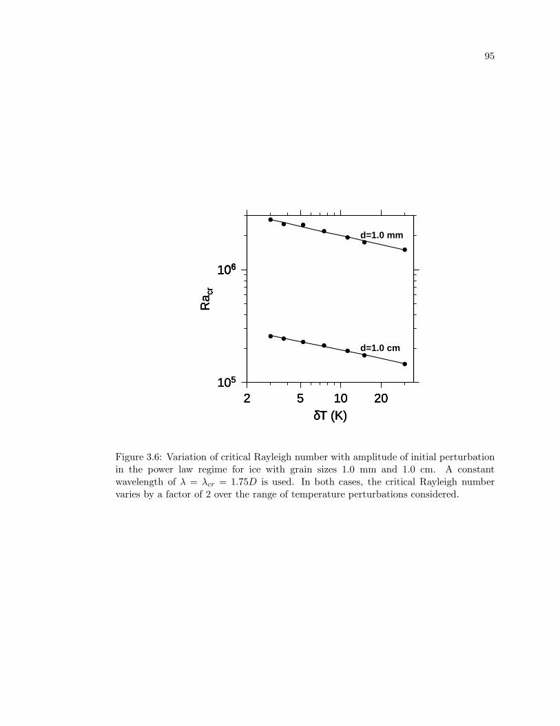
95

105

106106

Ra c

r

2 5 10 20δT (K)

105

106106

Ra c

r

2 5 10 20δT (K)

d=1.0 mm

105

106106

Ra c

r

2 5 10 20δT (K)

d=1.0 cm

Figure 3.6: Variation of critical Rayleigh number with amplitude of initial perturbationin the power law regime for ice with grain sizes 1.0 mm and 1.0 cm. A constantwavelength of λ = λcr = 1.75D is used. In both cases, the critical Rayleigh numbervaries by a factor of 2 over the range of temperature perturbations considered.

96

10-410-310-310-210-1100101102103104105106107

Ra c

r,0

10-5 10-410-4 10-3 10-2 10-1 100

Grain Size (m)

10-410-310-310-210-1100101102103104105106107

Ra c

r,0

10-5 10-410-4 10-3 10-2 10-1 100

Grain Size (m)

R2=0.9964

Figure 3.7: Fitting coefficient Racr,0 as a function of grain size. Dots indicate Racr,0

values obtained from fits to our numerical Racr data, and the line shows a third orderpolynomial fit to the data (equation 3.16) used to approximate the behavior of thefitting coefficient between data points. For grain sizes between 1.0 mm and 1.0 cm,the value of Racr,0 changes dramatically as the non-Newtonian deformation mechanismdislocation creep becomes activated, causing the viscosities in the ice shell to evolve tovalues much less than the reference viscosity.

97

d=0.1 mm

-0.8

-0.6

-0.4

-0.2

Dep

th

ηtotal

-0.8

-0.6

-0.4

-0.2D

epth

ηdiff

-0.8

-0.6

-0.4

-0.2

Dep

th

ηGSS

-0.8

-0.6

-0.4

-0.2

Dep

th

0.2 0.4 0.6 0.8X

ηdisl

d=1.0 mm

ηtotal

ηdiff

ηGSS

0.2 0.4 0.6 0.8X

ηdisl

d=1.0 cm

ηtotal

ηdiff

ηGSS

0.2 0.4 0.6 0.8X

ηdisl

13 14 15 16 17 18 19 20 21 22 23 24log 10 η (Pa s)

Figure 3.8: Maps of total viscosity in Pa s (top row), diffusional flow viscosity (secondrow), GSS viscosity (third row), and dislocation creep viscosity (bottom row) for threedifferent simulations with Rao = Racr, for increasing grain size from 0.1 mm (leftcolumn) to 1.0 cm (right column). A constant perturbation magnitude of 15 K wasused in each simulation, and the spatial coordinates are non-dimensionalized for ease ofcomparison. Under the composite flow law (equation 3.6), the deformation mechanismyielding the smallest viscosity (bluest) is dominant. As the grain size increases from0.1 mm (left panels) to 1.0 mm (center panels), the dominant deformation mechanismchanges from diffusional flow to GSS creep. As the grain size increases to 1.0 cm(right panels), dislocation creep becomes active and all three deformation mechanismscontribute to the total viscosity approximately equally. For grain sizes 0.1 mm and 1.0mm, the contribution to the total viscosity from dislocation creep is negligible becauseηdisl > 1024 Pa s, the maximum viscosity in the rigid ice near-surface ice.

98

plume is sufficient to activate dislocation creep. Figure 3.9 demonstrates the changing

role of dislocation creep for three simulations where Ra ∼ Racr as the grain size increases

from 1.0 cm to 3.0 cm. In this regime, convection can occur at much lower values of

Rao, but the value of effective Rayleigh number is still ∼ 106. As discussed in section

3.5, transitions in behavior with grain size are expected to have profound consequences

on the critical ice shell thickness for convection as grain size varies.

An expression for the critical ice shell thickness as a function of perturbation

amplitude and grain size in the power law regime can be obtained by combining the

scaling for critical Rayleigh number (3.17) and the definition of the Rayleigh number

(3.9) to obtain:

Dcr =

[

κηo

ρgα∆Texp

[

− 0.129(ln d)3 − 2.98(ln d)2 − 22.96(ln d) − 42.7]( δT

∆T

)−0.243]1/3

,

(3.18)

where the reference viscosity can be evaluated using equation (3.8).

In Chapter 2, we characterized the critical Rayleigh number for convection in ice

I with a GBS or basal slip rheology. The GBS deformation mechanism accommodates

deformation in ice I during the initial plume growth when the grain size of ice is approx-

imately 1 mm. Therefore, the results of our calculations here are consistent with the

results of Chapter 2 if the grain size of ice is assumed to be 1 mm. In this study, as in

our previous study, the conditions required to trigger convection in an ice I shell depend

strongly on the grain size of ice. In our previous work, when the GBS rheology was used,

changing the grain size of ice merely changed the value of the melting point viscosity.

Under the composite rheology, changing the grain size of ice changes the deformation

mechanism that accommodates convective strain.

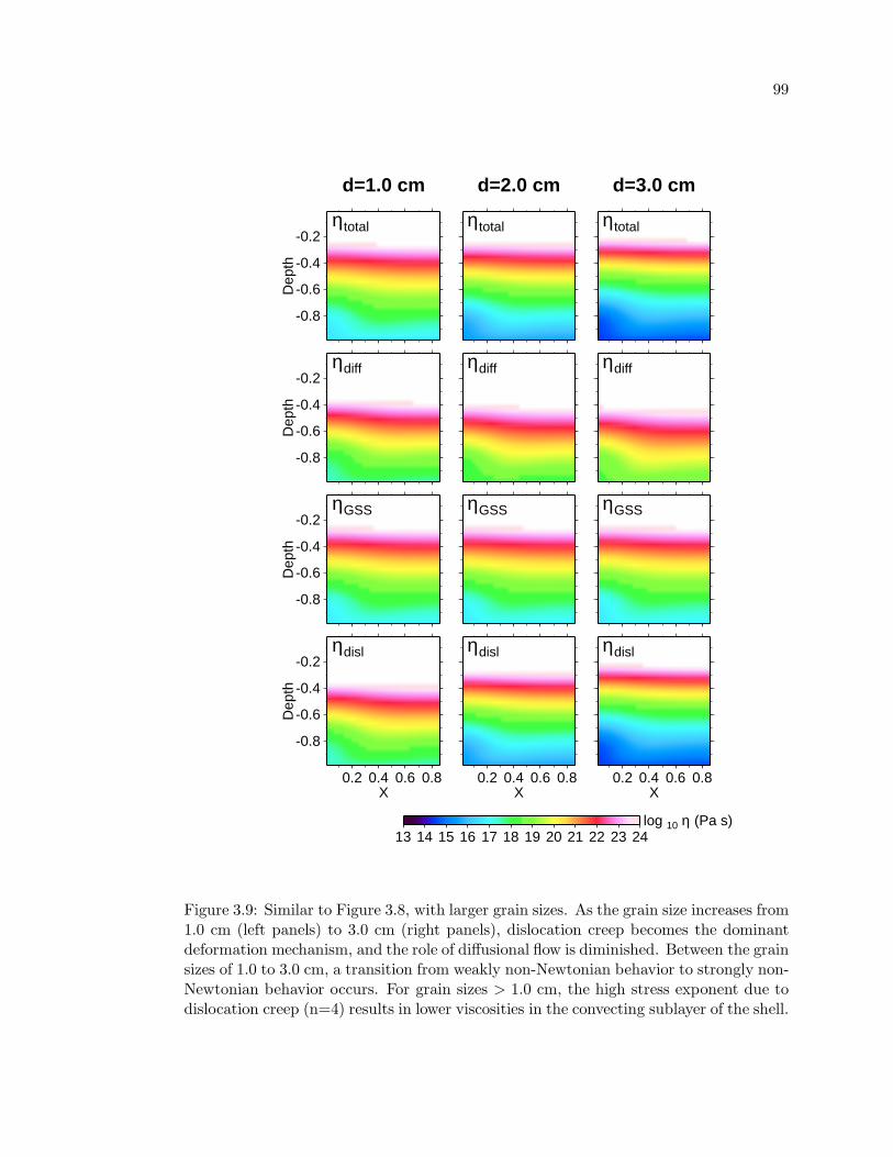
99

d=1.0 cm

-0.8

-0.6

-0.4

-0.2

Dep

th

ηtotal

-0.8

-0.6

-0.4

-0.2

Dep

th

ηdiff

-0.8

-0.6

-0.4

-0.2

Dep

th

ηGSS

-0.8

-0.6

-0.4

-0.2

Dep

th

0.2 0.4 0.6 0.8X

ηdisl

d=2.0 cm

ηtotal

ηdiff

ηGSS

0.2 0.4 0.6 0.8X

ηdisl

d=3.0 cm

ηtotal

ηdiff

ηGSS

0.2 0.4 0.6 0.8X

ηdisl

13 14 15 16 17 18 19 20 21 22 23 24log 10 η (Pa s)

Figure 3.9: Similar to Figure 3.8, with larger grain sizes. As the grain size increases from1.0 cm (left panels) to 3.0 cm (right panels), dislocation creep becomes the dominantdeformation mechanism, and the role of diffusional flow is diminished. Between the grainsizes of 1.0 to 3.0 cm, a transition from weakly non-Newtonian behavior to strongly non-Newtonian behavior occurs. For grain sizes > 1.0 cm, the high stress exponent due todislocation creep (n=4) results in lower viscosities in the convecting sublayer of the shell.

100

3.5 Implications for the Icy Galilean Satellites

Gravity and magnetic data from the Galileo mission suggest that Europa, Ganymede,

and Callisto have internal oceans, but the portion of their outer H2O layers that are

solid is loosely constrained. The maximum thickness of Europa’s ice-rich layer is approx-

imately 170 km (Anderson et al., 1998), but estimates based on geological observations

suggest that the solid ice shell is perhaps 20-25 km thick (Pappalardo et al., 1999; Nimmo

et al., 2003). For Ganymede and Callisto, the upper bound on ice I shell thickness is

obtained by estimating the depth to the minimum melting point of ice I in each satellite.

In Ganymede, assuming the shell is pure water ice with a density of 930 kg m−3, the

minimum melting point occurs at a depth of 160 km; in Callisto, 180 km.

The composite flow law used here is specific to water ice, so important caveats are

required before directly applying these results to the icy Galilean satellites. If impurities

such as hydrated sulfuric acids, hydrated magnesium salts, or ammonia are present in

the ice shells, the conditions for convection outlined here may not directly apply to the

Galilean satellites. Deviation in the rheological parameters due to the presence of these

or other materials could dramatically alter the rheology and the conditions required to

initiate convection. Additionally, we have assumed a constant grain size for the ice in

the shells, which is an oversimplification. Moreover, we have ignored internal heating

by tidal dissipation in favor of exploring the interesting changes in behavior with grain

size.

As discussed in section 3.3.1, we do not include the alternate set of rheological

parameters presented by Goldsby and Kohlstedt (2001) for enhanced creep rates due to

grain boundary sliding and dislocation creep caused by premelting at grain boundaries

and grain edges in ice near its melting point. If the high temperature creep enhancement

were included in the numerical model, the viscosities near the base of the ice shell

for grain sizes greater than 1.0 mm would be greatly reduced, potentially permitting

101

convection in thinner ice shells than determined in this study. As the initial convective

plumes if the convective temperature of the ice shell is within a few degrees of the

melting point, the entire sublayer of the ice shell would convect vigorously because of

its low viscosity. Additionally, if tidal dissipation warmed the sub-layer of an initially

conductive ice shell to a temperature close to the melting point, the sub-layer of the

shell could have a viscosity low enough to become convectively unstable. In this case, an

ice shell judged to be stable against convection in this study would convect if the high

temperature creep enhancement were included in the model. For this reason, it would

be valuable to include this high temperature creep enhancement in future modeling

efforts.

3.5.1 Conditions for Convection in Europa

Figure 3.10 illustrates the critical ice shell thickness for convection in Europa as a

function of grain size, employing equation (3.17) to interpolate between our Racr data

points. For all grain sizes, the critical shell thickness for convection is less than the

maximum permitted shell thickness. For a grain size of 0.1 mm, the thickness of ice

shell required to initiate convection is 14 km from an initial temperature perturbation

of 7.5 K spread over a characteristic distance roughly equal to the thickness of the

ice shell. The critical ice shell thickness maximizes at a value of 134 km for a 7.5 K

temperature perturbation at a grain size of 5 mm, where GSS creep is the dominant

deformation mechanism. For large grain sizes where the thermal stress of the plume

exceeds the transition stress from GBS to dislocation creep, the critical ice shell thickness

for convection is small. Under the composite rheology, an ice shell with the nominally

accepted thickness of 20-25 km (Pappalardo et al., 1999; Nimmo et al., 2003) can convect

given an initial perturbation of 15 K if the grain size is less than 0.3 mm or greater than

40 mm.

102

1

1010

100

Dcr

(km

)

10-4 10-310-3 10-2 10-1

Grain size (m)

1

1010

100

Dcr

(km

)

10-4 10-310-3 10-2 10-1

Grain size (m)

1

1010

100

Dcr

(km

)

10-4 10-310-3 10-2 10-1

Grain size (m)

Dmax = 170 kmDmax = 170 km

Figure 3.10: Critical ice shell thickness for convection in Europa as a function of grainsize. The bold line represents a perturbation amplitude of 3 K, the thin line representsa perturbation amplitude of 30 K. The dotted horizontal line represents the maximumpermitted shell thickness on Europa of 170 km.

103

3.5.2 Conditions for Convection in Ganymede and Callisto

Figures 3.11 and 3.12 illustrate the critical shell thickness for convection in Ganymede

and Callisto as a function of grain size. Similar to the Europa data, the critical shell

thicknesses for convection are less than the maximum permitted shell thickness in both

Ganymede and Callisto for the range of grain sizes considered here. If the ice shells of

Ganymede and Callisto are in conductive equilibrium with present-day radiogenic heat-

ing (4.5 ×10−12 W kg−1) (Spohn and Schubert , 2003) in their interiors, the equilibrium

ice shell thicknesses are 128 km and 148 km. Convection can occur in the present day

shells if the grain size is less than 6 mm or greater than 50 mm, given an initial temper-

ature perturbation of 15 K. Approximately 1.5 billion years ago when the concentration

of 40K was higher, and therefore radiogenic heating rates were twice their present val-

ues, the equilibrium ice shell thicknesses of Ganymede and Callisto were 64 km and 74

km, respectively. Convection could be triggered by a 15 K temperature perturbation in

these ancient, thin shells if the ice had a grain size less than 1 mm or greater than 17

mm.

3.5.3 Role of Tidal Heating

Tidal dissipation may play a key role in generating the ∼1-10’s K temperature

perturbations used as initial conditions in this study. Once the temperature pertur-

bation due to tidal dissipation reaches the rheological temperature scale ∼ 22 − 56 K

(see section 3.3.3, the critical Rayleigh number approaches a constant asymptotic value.

Therefore, adding additional tidal heat will not trigger convection in the ice shell and

could instead result in melting of the base of the shell.

Estimates of the total amount of energy dissipated by tidal flexing of Europa and

Ganymede’s ice shells exist, but the spatial distribution of the dissipation in their ice

shells is unknown. If tidal dissipation is spatially localized within convective upwellings

104

1

1010

100

Dcr

(km

)

10-4 10-310-3 10-2 10-1

Grain size (m)

1

1010

100

Dcr

(km

)

10-4 10-310-3 10-2 10-1

Grain size (m)

1

1010

100

Dcr

(km

)

10-4 10-310-3 10-2 10-1

Grain size (m)


Figure 3.11: Same as Figure 3.10, but for Ganymede.

105

1

1010

100

Dcr

(km

)

10-4 10-310-3 10-2 10-1

Grain size (m)

1

1010

100

Dcr

(km

)

10-4 10-310-3 10-2 10-1

Grain size (m)

1

1010

100

Dcr

(km

)

10-4 10-310-3 10-2 10-1

Grain size (m)


Figure 3.12: Same as Figure 3.10, but for Callisto.

106

on length scales similar to the thickness of the ice shell in convective upwellings (Tobie

et al., 2003), or along zones of weakness in the ice shell (Nimmo and Gaidos, 2002;

Tobie et al., 2004), the critical Rayleigh number for tidally triggered convection would

be similar to the values calculated here. It is also possible that the spatial pattern of

tidal dissipation within an ice shell follows the spatial distribution of the tidal strain

rate (Ojakangas and Stevenson, 1989). In this case, the wavelength of tidal dissipation

is much greater than the thickness of the ice shell, and much larger than the critical

wavelength used in our calculation. For wavelengths larger or smaller than the criti-

cal wavelength, the value of critical Rayleigh number is higher, and the critical shell

thickness for convection would be larger. Therefore, triggering of convection by tidal

dissipation could require a thicker ice shell than calculations here imply.

3.5.4 Evolution of Grain Size and Orientation

We have assumed a uniform grain size for the ice shell, which is certainly an

oversimplification for the icy satellites. Tidal heating, rapid tidal flexing of the ice

shells, and large convective strains likely modify the size and orientation of ice grains

in the shell.

By analogy with terrestrial ice sheets, ice shelves, and the Earth’s mantle, a

complex suite of processes is likely to occur within the ice shells to cause grain sizes

to evolve as a function of temperature, strain rate, impurity concentration, and total

accumulated strain. For example, flow by dislocation creep is likely to lead to smaller

grain sizes, whereas flow by grain boundary sliding or diffusional flow is likely to lead

to grain growth (e.g. De Bresser, et al., 1998). If grain growth or destruction occurs

in ice, the change in grain size may cause the rate-limiting deformation mechanism to

change as a function of the accumulated convective strain. Conclusions regarding the

convective stability of the ice shells drawn from this study are strongly dependent on

the grain size of ice. Therefore, we advocate using a more realistic grain size model

107

in future work, by allowing grain size to dynamically evolve as a function of depth,

temperature, stress and accumulated convective strain.

Additionally, consideration of the non-Newtonian deformation mechanisms may

present new opportunities to measure the behavior of the ice I shells with ice penetrating

radar. In addition to the evolution of grain size, the evolution of grain orientations can

have an effect on the radar reflectance properties of ice. Flow by volume diffusion

does not lead to the development of crystal fabric, where the orientation of ice grains

is constant over large regions in the ice shell (Karato et al., 1995). If volume diffusion

accommodates convective strain in the ice shell, a random distribution of grain sizes and

orientations will form. Therefore, existing numerical models of convection in ice I do

not predict the development of crystal fabric in the ice shells of the Galilean satellites.

Preferred orientation of the c axis of ice grains (crystal fabric) can lead to radar

polarization anisotropy in ice sheets (Matsuoka et al., 2003). Therefore, if large con-

vective strains in the ice shells are accommodated by deformation mechanisms that

lead to the development of crystal fabric (i.e. dislocation creep), radar polarization

anisotropy of the ice shell could be used to determine whether the ice shell convected.

If anisotropy due to crystal fabric could be deconvolved from other causes of radar po-

larization anisotropy in ice, and the pockets of coherent deformation are similar in size

to the wavelength of ice penetrating radar, radar sounding could potentially be used to

infer the strain history of the ice shell.

3.6 Summary and Conclusions

Recent laboratory experiments suggest that ice I exhibits a complex rheologi-

cal behavior at the temperatures and pressures appropriate to the interiors of the icy

Galilean satellites. Deformation in ice occurs due to several different creep mecha-

nisms, each of which become activated at different stresses and temperatures. At low

stresses, ice with a small grain size (∼ 0.1 mm) behaves as a Newtonian fluid, and de-

108

formation is accommodated by volume diffusion. As stress increases and temperature

drops, the rheology of ice becomes stress-dependent as the grain-size-sensitive creep

and dislocation creep mechanisms become active. The stresses associated with initial

plume growth within an ice I shell of the Galilean satellites are similar to the transition

stresses between several of the Newtonian and non-Newtonian deformation mechanisms,

necessitating inclusion of all mechanisms in a numerical convection model.

Using a composite Newtonian/non-Newtonian temperature and stress-dependent

rheology for ice I, we find that the critical ice shell thickness for convection is a strong

function of the grain size of the ice shell. We find that similar to a purely non-Newtonian

fluid, the critical ice shell thickness for convection in a composite Newtonian/non-

Newtonian ice shell depends on the amplitude of initial temperature perturbation issued

to the ice shell. A finite-amplitude perturbation (δT ∼1-10’s K) is required to initiate

convection regardless of the grain size of ice or thickness of ice shell. Tidal dissipation

may be required to generate such temperature perturbations.

Under the composite rheology, convection is possible in ice shells less than 30

km thick in Europa, Ganymede, and Callisto provided the grain size of ice is < 1 mm,

which allows diffusional flow to control plume growth, or > 1 cm, which allows thermal

stresses to activate non-Newtonian dislocation creep. For intermediate grain sizes, GSS

creep controls plume growth, in which case the critical ice shell thickness for convection

is close to the maximum permitted on the icy Galilean satellites, consistent with results

shown in Chapter 2 using a grain boundary sliding rheology.

Tidal dissipation likely plays a key role in initiating convection in the satellites, by

providing a source of temperature perturbations. However, because the physics of tidal

heating are poorly understood, we cannot judge whether the heat would be concentrated

in the ice shell over a horizontal length scale similar to the ice shell thickness, necessary

for tidal forcing to generate temperature perturbations similar to those used in this

study. If tidal heating is distributed over longer distances, thicker ice shells might be

109

required to permit convection from an initial temperature perturbation spread over a

large area.

Consideration of the non-Newtonian rheology of ice I has highlighted two very

important effects in judging the convective stability of the icy satellites that were pre-

viously unaddressed. As a result of the complex Newtonian/non-Newtonian behavior

of ice I, the conditions required to trigger convection in an ice shell depend on the

initial conditions in the shell and the grain size of ice. Given the requirement of a

finite-amplitude temperature perturbation to start convection, we postulate that tidal

dissipation plays a key role in softening the ice to permit convection and plan to focus

future studies toward the goal of understanding tidal heating in ice shells.

Chapter 4

Implications for the Internal Structure of the Major Satellites of the

Outer Planets

4.1 Abstract

As governed by the Goldsby and Kohlstedt (2001) composite Newtonian/non-

Newtonian rheology, the efficiency of convective heat transport in the outer floating

ice I shell of a large icy satellite is strongly dependent on the ice grain size. Basally

heated shells 20 - 100 km thick with assumed uniform grain size of ≤ 0.3 mm convect

vigorously with heat fluxes between 30-40 mW m−2 because Newtonian volume diffusion

accommodates convective strain and results in low ice viscosities in the convecting sub-

layer. If the ice has a grain size ≥ 30 mm, dislocation creep accommodates strain,

convection is sluggish, and convective heat fluxes are 15 - 20 mW m−2. When convection

occurs in the absence of tidal dissipation, the heat flux across an ice shell can exceed

the radiogenic heat flux, casuing the ice shell to thicken by meters per year. If the

ice shell has a grain size of 3-10 mm, it cannot convect if < 100 km thick, permitting

internal oceans to be thermodynamically stable in a Ganymede/Callisto-like satellite in

the absence of tidal dissipation or non-water-ice materials, given chondritic heating rates

appropriate for 1.5 billion years ago. If the melting point of the ice shell is depressed

due to the presence of non-water-ice materials such as sulfuric acid hydrate or ammonia,

oceans may be stable beneath conductive ice shells. If tidal dissipation occurs in the

ice I shell, additional heat may be supplied to the interior of the ice shell to balance

111

efficient convective heat transport, and may permit oceans to be thermodynamically

stable. If tidal dissipation is capable of changing the mode of heat transport across the

ice I shell, or the amount of tidal dissipation depends on the thermal structure of the

ice shell, the tidal and convective/conductive heat fluxes are linked quantities. More

detailed modeling of tidal dissipation is necessary to clarify how tidal heat is spatially

localized in the ice shell, and to investigate whether a feedback between tidal heating

and convection occurs.

4.2 Introduction

The results of Chapters 2 and 3 indicate that the critical Rayleigh number for

convection in ice I with a composite Newtonian/non-Newtonian rheology depends on

the amplitude and wavelength of initial temperature perturbation issued to an initially

conductive ice layer, in addition to the thermal, rheological, and physical parameters of

the ice shell. Here, we illustrate how the heat flux across a convecting ice shell depends

on the ice grain size, which determines the deformation mechanisms that accommodate

convective strain. We numerically model convection in basally heated ice shells using

a composite Newtonian and non-Newtonian rheology for ice I with uniform grain size

in the icy Galilean satellites to judge the thermodynamic stability of their liquid water

oceans.

4.3 Methods

4.3.1 Numerical Implementation of Ice Rheology

The laboratory experiments of Goldsby and Kohlstedt (2001) indicate that defor-

mation in ice I is accommodated by volume diffusion, dislocation creep, and grain size

sensitive (GSS) creep, the last of these occurring by both grain boundary sliding (GBS)

and basal slip (bs). The strain rate for each creep mechanism in the composite rheology

112

is described by

ε = Aσn

dpexp

(−Q∗

RT

)

, (4.1)

where ε is the strain rate; A, n, p, and Q∗ are experimentally determined rheological

parameters; d is the ice grain size, R is the gas constant, and T is temperature (Table

A.2).

Goldsby and Kohlstedt (2001) provide an alternate set of creep parameters for

GBS and dislocation creep in ice near its melting point, but we do not include this

effect in our present models. If the viscosities due to GSS and dislocation creep in the

warm basal ice are much smaller than described here, convection might be possible in

ice shells thinner than described by our models.

To implement a viscosity due to all four deformation mechanisms simultaneously,

we rephrase the composite flow law of Goldsby and Kohlstedt (2001) in terms of vis-

cosities using η = σ/ε, which allows an approximate solution for the total viscosity (see

Chapter 3):

ηtot =

[

1

ηdiff+

1

ηdisl+

(

ηbs + ηGBS

)−1]−1

. (4.2)

An explicit stress-dependent rheology of form

η =dp

Aσ(1−n) exp

( Q∗

RT

)

(4.3)

is used for each term in equation (4.2). To non-dimensionalize the rheology, we divide

each term in equation (4.2) by the viscosity due to diffusional flow at the melting

temperature of ice,

ηo =d2

Aexp

( Q∗v

RTm

)

. (4.4)

The transition stresses between the deformation mechanisms are mathematically rep-

resented by a series of weighting factors (β) between the four component rheologies,

which govern the relative importance of each mechanism as a function of temperature

and grain size (see Chapter 3). Values of the weighting factors appropriate for the val-

ues of grain size used in this study are listed in Table B.7. Each viscosity function is

113

expressed in non-dimensional coordinates (primed quantities) as:

η′ =1

βσ′(1−n) exp

( E

T ′ + T ′o

−Ev

1 + T ′o

)

(4.5)

where σ′ = σ/(ηoεo) is non-dimensional stress, E = Q∗/nR∆T is the non-dimensional

activation energy, Ev = Q∗v/nR∆T , and T ′

o = Ts/∆T is the reference temperature.

Thermal and physical parameters used in this study are summarized in Table A.1.

We use a reference Rayleigh number defined by

Rao =ρgα∆TD3

κηo, (4.6)

where ρ = 930 kg m−3 is the density of ice, g is the acceleration of gravity, α = 10−4

K−1 is the coefficient of thermal expansion, ∆T is the temperature difference between

the surface and base of the shell, and κ = 10−6 m2 s−1 is the thermal diffusivity. In a

non-Newtonian fluid, viscosities in the layer may evolve to values larger or smaller than

ηo depending on the vigor of convection. The viscosity at the melting point near the

base of the ice shell is 1013 Pa s when volume diffusion and dislocation creep are the

dominant rheologies. When GSS creep accommodates convective strain, the viscosity

in the convecting interior of the ice shell is 1014 to 1015 Pa s.




the governing equations of thermally-driven convection in an incompressible fluid. Our

simulations are performed in 2D Cartesian geometry, and free-slip boundary conditions

are used on the surface (z = 0), base (z = −D), and side walls (x = 0, xmax) of the do-

main. All simulations in this chapter are performed in a domain with 64 x 64 elements,

chosen to resolve the thermal boundary layers while allowing sufficient coverage of our

parameter space given limited computational resources. All simulations are run until

the surface heat flux converges to within 0.01% per time step.

114

The layer is purely basally heated, so internal heating by tidal dissipation is not

considered in our numerical models, and is briefly discussed in section 4.4.5. The surface

of the convecting layer is held at a constant temperature of Ts = 110 K, appropriate for

the equatorial surfaces of an icy Galilean satellite, and the base of the ice shell is kept

at the melting point of water ice, assumed constant at Tm = 260 K.


Each simulation is started from a uniform initial condition of a conductive equi-

librium plus a temperature perturbation expressed as a Fourier mode:

T (x, z) = Ts −z∆T

D+ δT cos

(2πD

λx

)

sin

(−zπ

D

)

, (4.7)

where λ = D and δT = 7.5 K. If convection does not occur with δT =7.5 K, an

additional simulation is performed with δT=37.5 K. In most cases where convection

does not initiate from an initial temperature perturbation of 7.5 K, convection does not

initiate from the larger perturbation either. When D = 60 km and d = 1.0 mm, we find

that Rao ∼ Racr and convection is triggered in the shell with a perturbation of 37.5

K, but not from the smaller 7.5 K perturbation. In this case, convection is extremely

sluggish, confined to the bottom 40% of the shell.

4.4 Thermodynamic Stability of Oceans

If the heat flux across the ice shell due to conduction and convection exceeds the

radiogenic and potentially tidal heating, the liquid water layer in the satellite will freeze

and the ice shell will thicken. The heat flux due to convection is given by

Fc =k∆T

DNu, (4.8)

where k = 3.3 W m−1 s−1 is the thermal conductivity, and Nu is the Nusselt number

which expresses the relative efficiency of convection (Nu > 1) over conduction (Nu ≡ 1).

115

Under the composite rheology, the relationship between the Rayleigh number and the

Nusselt number (Nu = aRab) implicitly relates the thickness of the ice shell and grain

size to the convective heat flux. To properly determine the Nusselt number for the ice

shell, we must first determine whether convection occurs, then determine the steady

state heat flux across the ice shell for cases where convection does occur.

4.4.1 Critical Rayleigh Number

Our studies of the critical Rayleigh number for convection in ice I described in

Chapter 3 indicate that the critical ice shell thickness required for convection depends

on the grain size of ice, which controls the deformation mechanism that accommodates

strain during initial plume growth. For small grain sizes (0.1-1 mm), Newtonian volume

diffusion accommodates strain, and convection can occur in relatively thin ice shells

D < 35 km. For large grain sizes (d > 10 mm), dislocation creep accommodates strain,

and the large stress exponent permits the ice in the warm convecting sublayer of the ice

shell to have a relatively low viscosity once convection begins. For intermediate grain

sizes (3 mm < d < 10 mm), the critical ice shell thickness for convection is greater than

100 km.

4.4.2 Efficiency of Convection

To characterize the Nusselt number for convecting ice shells, we perform numerical

simulations of convection to determine Nu for a range of values of ice grain size from 0.1

to 30 mm, and ice shell thickness from 20 to 100 km. Rayleigh numbers for the ice shells

are calculated using an acceleration of gravity g = 1.3 m s−2. This value is appropriate

for Europa, and mid-way between values for Ganymede and Callisto. Figure 4.1 shows

the parameter space explored, and which parameter sets resulted in convection. The

scaling between critical ice shell thickness and grain size from Chapter 3 using λ = 1.75D

is shown on Figure 4.1 as well. The relationship between Dcr and d derived in Chapter

116

20

40

60

80

100

D (

km)

10-410-4 10-3 10-2 10-1

d (m)

20

40

60

80

100

D (

km)

10-410-4 10-3 10-2 10-1

d (m)

20

40

60

80

100

D (

km)

10-410-4 10-3 10-2 10-1

d (m)

20

40

60

80

100

D (

km)

10-410-4 10-3 10-2 10-1

d (m)

Figure 4.1: Parameter space of grain size (d) and ice shell thickness (D) explored inthis study. Crosses indicate that convection did occur in the ice shell, triggered from aninitial temperature perturbation of 7.5 K. Filled squares indicate that convection did notoccur, even when the temperature perturbation was 37.5 K. The solid line represents thescaling between critical shell thickness and grain size for a temperature perturbation of7.5 K (from Chapter 3) which is approximately correct for the wavelength and numericalresolution used here. For the open square with cross, D=60 km and d=1 mm, Ra ∼Racr, and convection was initiated from a temperature perturbation of 37.5 K, but notfrom the smaller 7.5 K perturbation.

117

3 is only approximately correct for λ = 2.0D, because the numerical resolution of the

critical Rayleigh number calculations in Chapter 3 was 32x32 elements, whereas here we

use a higher resolution of 64x64 elements. Doubling the numerical resolution affects the

value of critical Rayleigh number at the 10% level. Additionally, the critical Rayleigh

number is a weak function of λ under the composite rheology of ice, so the stability

curve for λ = 1.75D is slightly different (at the 5% level) than the stability curve for

λ = 2.0D.

Table 4.1 summarizes the values of Nusselt number and convective heat flux

obtained from our simulations where convection occurred. The grain size of ice controls

the value of Nu by controlling which rheologies are active in the ice shell after the

initial plumes grow into a well-developed convection pattern. The convective heat flux

is only weakly dependent on the thickness of the ice shell, consistent with the behavior

of stagnant lid convection. For a grain size of 0.1 mm, volume diffusion accommodates

deformation and viscosities in the shell are generally low. This leads to efficient heat

transport by convection and large heat fluxes of order 30 - 40 mW m−2 (2 < Nu < 6).

As the grain size increases to 0.3 mm, the viscosity of ice increases by a factor of 10, as

GSS creep becomes activated. Resultant convective heat fluxes are halved, with values

ranging from 15 - 20 mW m−2 (2 < Nu < 1).

To compare our results to recent calculations by Spohn and Schubert (2003) that

employ parameterized convection models using Newtonian rheologies to address the

thermodynamic stability of oceans, we fit our Ra − Nu data to an equation of form:

Nu = aRabo. We find that a ranges from 0.01 to 0.05 and values of b range from 0.26 to

0.3 for 0.1 mm < d < 1 mm. Our values of b are consistent with the values of b used by

Spohn and Schubert (2003) (0.2 < b < 0.3). However, our vales of a are substantially

smaller, which is likely due to the difference in our definition of Rayleigh number, which

is evaluated at the melting temperature of ice, rather than the interior temperature of

the ice shell (Spohn and Schubert , 2003).

118

Table 4.1: Convective Heat Flux and Nu for 20 km < D < 100 km

D (km) d (m) Rao Nu Fconv (mW m−2)

20 10−4 5.9 × 106 1.67 4120 10−3 3.1 × 106 1.57 39

35 10−4 3.2 × 107 2.15 3035 3 × 10−4 3.5 × 106 1.60 2335 3 × 10−2 3.5 × 102 1.53 22

50 10−4 9.2 × 107 3.51 3550 3 × 10−4 1.0 × 107 1.85 1850 3 × 10−2 1.0 × 103 1.79 18

60 10−4 1.6 × 108 4.07 3460 3 × 10−4 1.8 × 107 2.05 1760 10−3 1.6 × 106 1.16 9.560 3 × 10−2 1.8 × 103 1.98 16

75 10−4 3.1 × 108 5.36 3575 3 × 10−4 3.5 × 107 2.45 1675 3 × 10−2 3.5 × 103 2.11 14

85 3 × 10−2 5.0 × 103 2.69 1685 3 × 10−4 5.0 × 107 2.69 16

100 3 × 10−4 8.2 × 107 3.37 17100 10−3 7.4 × 106 1.76 8.7

119

4.4.3 Ocean Stability Without Tidal Heating

To judge the thermodynamic stability of the oceans, we use the conductive and

convective heat flux (Fc) data described above to calculate an instantaneous rate of

change of the thickness of the ice shell from the net heat flux across the shell. In the

absence of tidal dissipation, Fnet=Fc−Fr, where Fr is the radiogenic heat flux. The rate

of change of the thickness of the ice shell is evaluated by equating the heat required to

freeze a layer δD thick at the bottom of an ice shell to the net amount of heat removed

from the ice shell by convection and conduction in a time δt:

4π(Rs − D)2δDρHf = (Fc − Fr)4πR2sδt, (4.9)

where Rs is the radius of the satellite, Hf = 3.3 × 105 J kg−1 is the heat of fusion of

ice, and δD/δt is approximated by assuming D/Rs ≪ 1,

δD

δt∼

Fc − Fr

ρHf. (4.10)

Positive values of δD/δt indicate that the ice shell is thickening; negative values indicate

that the ice shell is melting.

In this formulation, the excess heat flux from the ice shell by efficient convec-

tive heat transfer is assumed to be removed from the ocean, thereby causing freezing.

Therefore, this analysis of the heat balance between radiogenic heating and the con-

vective/conductive heat flux is only appropriate to non-tidally-heated satellites such

as Ganymede at present, and Callisto. It is not directly applicable to Europa, where

tidal dissipation exceeds the radiogenic heat flux and dominates the heat budget of the

satellite.

We calculate growth rates for a Ganymede- or Callisto-like satellite using a present

chondritic heat flux midway between values for Ganymede and Callisto as estimated by

Spohn and Schubert (2003). The chondritic heat flux appropriate for 1.5 billion years

in the past is approximately twice the present value due to the increased concentration

120

of 40K. We use Fr=3.6 mW m−2 for the present chondritic heat flux and Fr=7.2 mW

m−2 for 1.5 billion years ago.

Figure 4.2 shows the heat flux across the ice shell as a function of grain size and

shell thickness, and rates of change of shell thickness in a Ganymede/Callisto-like body

1.5 billion years ago and at present. Growth or thinning rates of the ice shells are of

order meters per year, and an ocean could persist without thinning (i.e. δD/δt=0) in

a Ganymede/Callisto-like satellite 1.5 billion years ago if the ice shell is 68 km thick.

At present, pure water-ice oceans in the satellites will be slowly freezing regardless of

whether the ice shell convects or not. When the ice shells are thick enough to convect,

at present, oceans in the Ganymede/Callisto-like body are freezing at a rate of 0.2 m

yr−1 to 3 m yr−1, depending on shell thickness and grain size.

As the thickness of the ice shell increases to a value where convection is per-

mitted, convection may occur if the ice shell is issued a finite-amplitude temperature

perturbation with λ ∼ λcr, so that Ra ∼ Racr. If convection begins, the rate of freezing

will increase because of the relative efficiency of convection over conduction, resulting

in freezing of the ocean unless additional heat by tidal dissipation or non-water-ice

materials dissolved in the ice shell depress its freezing point.

4.4.4 Presence of Non-Water-Ice Materials

Non-water ice materials such as ammonia and sulfuric acid in the shell can modify

the melting point of the shell and potentially permit stable oceans in the absence of tidal

dissipation in non-tidally heated satellites like Callisto. The melting point of the ice

shell could be depressed due to the presence of several non-water-ice materials. The

presence of ammonia in the ice shell can depress the freezing point of an ammonia-

water ocean to 176 K (Spohn and Schubert , 2003). The presence of H2SO4·nH2O, can

depress the freezing point of water to 211 K (Kargel et al., 2000). When the ocean is

stable, Fc = Fr, and we can solve for the melting point of the ice shell that would permit

121

0

15

30

45

Hea

t Flu

x (m

W m

-2)

20 40 60 80 100D (km)

0

15

30

45

Hea

t Flu

x (m

W m

-2)

20 40 60 80 100D (km)

0

15

30

45

Hea

t Flu

x (m

W m

-2)

20 40 60 80 100D (km)

0

15

30

45

Hea

t Flu

x (m

W m

-2)

20 40 60 80 100D (km)

0

15

30

45

Hea

t Flu

x (m

W m

-2)

20 40 60 80 100D (km)

0

1

2

3

0.1 mm

0.3 mm

30 mm

1.0 mm

3.0 mm - 10 mm 0

1

2

3

4

δD/δ

t (m

yr-1

)

Present1.5 Gya

Figure 4.2: Convective heat flux as a function of ice shell thickness, with superimposedrates of shell thickening (δD/δt > 0) or thinning (δD/δt < 0) for various grain sizes aslabeled from 0.1 - 30 mm. Growth rates for the ice shell range from -0.75 to 3.9 m yr−1

1.5 billion years ago and -0.37 to 4.25 m yr−1 at present (far right axis).

122

a stable ocean:

Tm = Ts +FrD

kNu. (4.11)

We are not able to evaluate this expression for convective ice shells because the rheology

of ice, values of Rayleigh number, and therefore, the relationship between the Nusselt

number and convective heat flux are calculated assuming Tm = 260 K and pure water

ice. However, if the ice shell does not convect and Nu = 1, Tm = 176 K (the ammonia-

water eutectic temperature) would permit an ocean to be stable beneath an ice shell

60.5 km thick in a Callisto-like satellite at present, and Tm = 220 K would permit a

stable ocean beneath a 100 km thick shell. One and a half billion years in the past,

Tm = 176 K would permit a stable ocean beneath a 30 km thick shell, and Tm = 220 K

would permit a stable ocean beneath a 50 km thick ice shell.

4.4.5 Tidal Dissipation

If tidal dissipation is occurring in the ice shell of the satellite, additional heat will

be supplied to the interior of the satellite which may decrease the rate of ocean freezing,

or prevent it from freezing, even if convection is occurring. With tidal dissipation

included, the net heat flux across the ice shell is:

Fnet = Fc − Fr − Ftidal. (4.12)

The rate of energy dissipation within a satellite in eccentric orbit around its parent body

is given by (Peale and Cassen, 1978):

E =21

2

k

Q

R5sGM2

Jne2

a6, (4.13)

where k is the Love number describing the response of satellite’s gravitational potential

to the applied tidal potential, Rs is the radius of the satellite, G is the gravitational

constant, MJ is the mass of the parent planet, n is the satellite’s mean motion, e is the

orbital eccentricity, Q is the tidal quality factor describing the fractional orbital energy

123

dissipated per cycle, and a is the semi-major axis of the satellite’s orbit about the parent

body.

The Love number k describes the response of the satellite to the tidal deformation,

and can only be approximated, because the value will depend on the distribution of mass

within the satellite, the rigidity of the ice shell, and the viscosity of the ice. If Europa

has a thin floating ice shell, k 0.25 (Moore and Schubert , 2000). If the satellite does not

have an internal ocean, and the ice I layer is rigidly coupled to the rock or ice layers

within the satellite, k becomes very small. Because the tidal dissipation is proportional

to k, and k ∼ 0 for a satellite without an internal water ocean, it is likely that tidal

dissipation in an icy satellite can only help to maintain an ocean, not create an ocean.

Values of the tidal quality factor are not well-constrained, but Q ∼ 100 is com-

monly assumed for the icy satellites (Murray and Dermott, 1999 and references therein.)

The actual value of Q for the satellite will depend on the amount of non-recoverable

viscous deformation that occurs within the satellite over one orbital cycle. For a vis-

coelastic satellite, the Love number k is complex, and the amount of energy lost per

cycle is proportional to the imaginary part of k (Segatz et al., 1988):

E =21

2Im(k)

(nRs)5

Ge2. (4.14)

In Europa and Ganymede, tidal dissipation may serve as an important heat source

in the outer ice I shells because the viscosity of ice near its melting point is potentially

small enough to permit a significant amount of non-recoverable viscous deformation in

the ice shell over each orbital cycle of the satellite. The value of Im(k) will depend

critically on the temperature-dependent rheology of the ice shell. Therefore, the overall

temperature structure of the ice shell could affect the value of Im(k). As a result, a

thick convecting ice shell with a sub-layer warmed to near its melting point could be a

more dissipative state than a cold conductive shell. In a convective shell, the sub-layer of

the shell could undergo appreciable viscous deformation due to tidal flexing of the shell

124

over a single orbital cycle, causing the total amount of tidal dissipation could increase.

In this way, the heat flux across the ice shell (Fc), which depends on whether convection

occurs or not, and the tidal heat flux (Ftidal) in equation (4.12) are linked quantities.

It is uncertain whether an equilibrium between dissipation in the ice shell and

the convective heat flux exists. If the tidal heat flux is greater than the maximum

convective heat flux, which is controlled by the rheology of the ice, the ice shell will

thin and convection will cease. If the tidal heat flux is less than the convective heat

flux, the ice shell will thicken, convection will become more vigorous, and the ocean

will freeze quickly. If the ice shell is thick, but initially conductive, tidal heating can

potentially trigger convection in the ice shell, and the evolution of the ice shell and

ocean will depend on the existence of an equilibrium between the heat flux due to tidal

dissipation and the convective heat flux.

Simple estimates of the rate of energy dissipation given assumed values of k and

Q can shed some light on the role that tidal dissipation might play in maintaining an

ocean beneath a floating ice shell in Ganymede and Europa. The energy dissipation

rate for Ganymede with its present semi-major axis is approximately (cf. Showman and

Malhotra, 1997):

Ftidal =E

4πR2s

= 2 × 107 mW m−2

(

e2k

Q

)

. (4.15)

Descriptive parameters of Ganymede’s orbit used to evaluate equation (4.13) to obtain

equation (4.15) are summarized in Table 4.2. Using k ∼ 0.25 and Q ∼ 100, the energy

dissipation rate at present in Ganymede given its present eccentricity of 0.0015 (Murray

and Dermott , 1999) is approximately 0.1 mW m−2, a factor of 20 less than the present

radiogenic heat flux, and a factor of 50 less than the radiogenic heat flux 1.5 billion

years ago. Ganymede may have experienced a period of increased orbital eccentricity

during passage through resonances with Europa and Io. During resonance passage,

the eccentricity of Ganymede’s orbit may have increased to ∼ 0.01, assuming a Q for

125

Table 4.2: Descriptive Parameters of the Orbits of Europa and Ganymede, from Murrayand Dermott (1999). †Values from Showman and Malhotra (1997).

Description Symbol Europa GanymedePresent Resonance†

Love Number k 0.25 0.25 0.25Tidal Quality Factor Q 100 100 100Radius of Satellite (km) Rs 1561 2634 2634Mass of Jupiter (kg) MJ 1.898 ×1027 1.898 ×1027 1.898 ×1027

Mean Motion (s−1) n 2 × 10−5 10−5 10−5

Eccentricity e 0.01 0.0015 0.01Semi-major Axis (km) a 6.71 × 105 1.07 ×106 1.07 ×106

Jupiter of 3 × 105 (Showman and Malhotra, 1997). During this time, the surface heat

flux due to tidal dissipation would have been 6 mW m−2, approximately equal to the

chondritic heat flux appropriate for 1.5 billion years ago. The enhanced heating during a

resonance passage would permit stable oceans beneath ice shells with heat fluxes below

Fr + Ftidal = 13.2 mW m−2. During Ganymede’s passage through an orbital resonance,

an ocean could be thermodynamically stable beneath a conductive ice shell 36 km thick.

The surface heat flux due to tidal dissipation at present in Europa is approxi-

mately:

Ftidal = 2 × 108 mW m−2

(

e2k

Q

)

. (4.16)

Using values of k = 0.25, Q = 100, and e = 0.01 (see Table 4.2), the surface heat flux is

approximately 50 mW m−2, which is a factor of 5 larger than the estimated chondritic

heat flux of 11 mW m−2 for Europa 1.5 billion years ago, and a factor of 10 larger than

the present chondritic heat flux of ∼ 5 mW m−2 (Spohn and Schubert , 2003). This

large heat flow also exceeds the maximum value of convective heat flux appropriate

for a basally heated ice shell obtained for D = 20 km in our study, indicating that

if the tidal dissipation were concentrated at the base of Europa’s ice shell, a 20 km

thick shell would not be thermodynamically stable, even if convection provided efficient

heat transfer. The majority of Europa’s tidal dissipation likely occurs in the ice shell,

126

because the viscosity of Europa’s ice shell is low enough to permit appreciable non-

recoverable viscous deformation over one Europan orbital cycle. Given the overwhelming

contribution of tidal dissipation to Europa’s total heating budget, detailed modeling of

tidal dissipation in Europa’s ice shell is required to quantify how tidal heat helps to

maintain Europa’s ocean.

4.5 Summary

Basally heated shells between 20 - 100 km thick with uniform grain size convect

vigorously when the grain size of ice is small, 0.3 mm or less, and Newtonian volume dif-

fusion accommodates convective strain. The composite Newtonian and non-Newtonian

behavior of the ice shell predicts sluggish convection or no convection in ice with grain

sizes 3-10 mm, due to large viscosities of ice when deformation is accommodated by

GSS creep. If the ice has a grain size ≥ 30 mm, dislocation creep accommodates strain,

convection is vigorous in ice shells thicker than 30 km.

Basally heated shells between 20 - 100 km thick with uniform grain size convect

vigorously with heat fluxes between 30-40 mW m−2 when the grain size is less than 0.3

mm. If the ice has a grain size ≥ 30 mm convective heat fluxes are between 15-20 mW

m−2. When convection occurs, the heat flux across the shell exceeds the radiogenic heat

flux, and the ice shells thicken by meters per year. If the ice shell does not convect,

liquid water oceans can be thermodynamically stable in the absence of tidal heating

or non-water-ice materials in a Ganymede- and Callisto-like body 1.5 billion years ago

when radiogenic heating was increased. If the melting point of the ice shell is modified

by the presence of non-water-ice materials such as ammonia and sulfuric acid hydrate,

oceans could be stable beneath thinner, non-convecting ice shells. Evaluation of the

stability of oceans beneath convecting ice shells with non-water-ice materials included

requires modification of the rheology of the ice shell to account for the difference in

melting temperature (Tm 6= 260 K) and potential modification of the grain size of ice

127

and rheology of ice.

Given the overwhelming contribution of tidal dissipation to Europa’s total heat

budget, it is likely that tidal heating helps to maintain a thermodynamically stable ocean

beneath Europa’s floating ice shell. If the heat flux due to tidal dissipation exceeds the

maximum permitted convective heat flux (which is a function of the ice rheology), tidal

dissipation may cause the ice shell to thin. A potential feedback between the thermal

and rheological structure of Europa’s ice shell precludes making conclusions about the

stability of Europa’s ocean or the thickness of its ice shell using our numerical results. If

Ganymede experienced widespread internal melting during passage through an orbital

resonance in the past, tidal dissipation in the ice shell may have caused the ocean to

grow. However, at present, tidal dissipation in Ganymede is a small contribution to

its total heat budget, indicating that non-water-ice materials may prevent freezing of

its ocean. Because Callisto has not experienced any tidal dissipation, our calculations

indicate that its ocean must be maintained due to the presence of non-water-ice materials

that depress the freezing point of its ice shell.

The heat balance arguments presented here are broadly consistent with the results

of Spohn and Schubert (2003). However, the key departure between our models and

existing studies lies in the behavior of the ice I shell during the onset of convection,

wherein convection must be triggered by a finite-amplitude temperature perturbation

to the ice shell. If tidal dissipation can be concentrated on horizontal spatial scales

similar to the thickness of the ice shell (i.e. λtidal ∼ λcr), convection may be triggered

by tidal heating. However, the detailed physics of how tidal dissipation occurs in the ice

shells is not well understood. Therefore, the potential for tidal dissipation to change the

mode of heat transport by triggering convection or thinning the ice shells is unknown,

and depends on the rheology of the ice. For this reason, the modeling described here is

a necessary first step toward building more realistic models of tidal dissipation in the

icy satellites.

Chapter 5

Implications for Astrobiology

5.1 Abstract

Solid state convection and endogenic resurfacing in the outer ice I shells of the

icy Galilean satellites may contribute to the habitability of their internal oceans and to

the detectability of biospheres by spacecraft. If convection occurs in an ice I layer, fluid

motions are confined beneath a thick stagnant lid of cold, immobile ice that is too stiff

to participate in convection. The thickness of the stagnant lid varies from 30 to 50% of

the total thickness of the ice shell, depending on the grain size of ice. Upward convective

motions deliver 109 to 1013 kg yr−1 of ice to the base of the stagnant lid where resurfacing

events driven by compositional or tidal effects such as the formation of domes or ridges

on Europa may deliver materials from the stagnant lid onto the surface. Conversely,

downward convective motions deliver 109 to 1013 kg yr−1 of ice from the base of the

stagnant lid to the bottom of Europa’s ice shell. Materials from the surface of Europa

may be delivered to the ocean by downward convective motions if material from the

surface can reach the base of the stagnant lid during resurfacing events. Triggering

convection in an initially conductive ice I shell requires modest amplitude (a few to 10’s

K) temperature anomalies to soften the ice to permit convection, which may require

tidal dissipation. Therefore, tidal dissipation, compositional buoyancy, and solid-state

convection may be required to permit mass transport between the surfaces and oceans

of the satellites.

129

5.2 Introduction

The outer ice I shells of icy satellites serve as a physical barrier between remote

sensing instruments and their internal liquid water oceans. The ice I shell is also barrier

between chemical nutrients generated on the surfaces of the satellites and the internal

oceans. Therefore, the understanding the geophysical processes that transport possible

life, nutrients, and the chemical traces of life between their ice-covered oceans and

surfaces is relevant to determining whether a biosphere can be sustained within and

detected on the icy Galilean satellites.

Solid state convection is potentially an important process in contributing to mass

transport across the ice I shell. When convection occurs in an ice I layer, convective

motions are confined beneath a stagnant lid of cold ice which limits the efficiency of

convective heat transfer and seemingly prevents convective motions from reaching the

surface of the ice shell (Barr and Pappalardo, 2003). The extent to which convection

and resurfacing permit mass exchange between the surface and ocean is addressed by

three geophysical questions:

• Under what conditions can convection occur in the outer ice I shells of the icy

Galilean satellites?

• If convection occurs in the ice I shells, what is the efficiency of mass transport

beneath the stagnant lid?

• How might the stagnant lid be breached?

Here, we summarize the astrobiological setting of the Galilean satellites, and ad-

dress the above questions using results obtained from previous chapters. The conditions

required to trigger convection in an ice I shell are determined in Chapter 3, with key

results summarized here. The numerical results used to determine the efficiency of con-

vective heat transfer described in Chapter 4 are used to characterize the mass flux of

130

ice recycled by convection beneath the stagnant lid. Finally, we discuss the formation

of ridges and domes on Europa as possible methods of breaching the stagnant lid.

5.3 Astrobiological Setting

The top panel of Figure 5.1 summarizes the geophysical processes that may en-

hance the habitability of Europa’s ocean. Because Europa’s ocean is cut off from sunlight

by kilometers of ice, any life in the ocean must be dependent upon delivery of nutrients

from the ice shell or from volcanic eruptions on Europa’s rocky mantle. Although it

is possible that microbial communities could be sustained through chemical reactions

which do not rely on the circulation of the ice shell (i.e. at deep hydrothermal vents)

(Jakosky and Shock , 1998; McCollom, 1999; Zolotov and Shock , 2004), the chemical en-

ergy available to organisms using these reactions may be small compared to the amount

of energy available in a radiation-driven ecosystem.

Based on predictions of impactor flux and the observed number of craters larger

than 10 km, the nominal age of Europa’s surface is ∼ 50 Myr, with an uncertainty of a

factor of 5 (Zahnle et al., 1998; Pappalardo et al., 1999; Zahnle, 2001). If the material

within Europa’s ice shell is mixed into the ocean on time scales similar to the surface

age, radiation-based nutrient sources could be made available to potential organisms in

the ocean.

Radioactive decay of 40K within the ice shell could generate up to ∼ 108 mol yr−1

of O2 and H2, which could chemically equilibrate in the ocean and sustain ∼ 106 cell

cm−3 of biomass over a 107 year timescale (Chyba and Hand , 2001). Formaldehyde,

hydrogen peroxide, and other materials are produced on the surface of Europa when

particles entrained in Jupiter’s magnetic field interact with H2O and CO2 ices (Carlson

et al., 1999). These materials have been spectroscopically detected on Europa’s surface

(Carlson et al., 1999). Products of radiation chemistry near the surface are expected to

be well mixed to a depth of 1.3 meters (Cooper et al., 2001). The steady-state biomass

131

that could be sustained by the equilibration of formaldehyde and hydrogen peroxide is

estimated to be ∼ 1023 cells (Chyba and Phillips, 2002), or 0.1 to 1 cell cm−3, assuming

the top 1.3 meters of ice is transported to the ocean every 107 years.

The basic elemental building blocks of life and additional nutrients for life may

be delivered to Europa through cometary impacts. Although a large percentage of

the ejecta from a large impact exceeds Europa’s escape velocity, at least 1012 to 1013

kg of carbon, and 1011 to 1012 kg of nitrogen, sulfur, and phosphorous may have been

delivered to Europa’s surface by giant impacts over the age of the solar system (Pierazzo

and Chyba, 2002). Endogenic resurfacing events coupled with downward motion of ice

in a convecting ice shell would be required to deliver these materials to Europa’s ocean.

Abundant endogenic resurfacing and active tidal dissipation on Europa suggests

that among the large icy satellites in our solar system, Europa holds the most potential

for finding life or interesting chemistry near the surface. The formation of surface

features such as domes (Pappalardo and Barr , 2004) and ridges (Nimmo and Gaidos,

2002) on Europa may allow small areas of the surface materials to be mixed into the

subsurface, but an ongoing global mechanism to breach the stagnant lid is required to

sustain a biosphere.

The bottom panel of Figure 5.1 summarizes the geological processes relevant to

astrobiology in Ganymede and Callisto. Unlike an ocean within Europa, which may

be in direct contact with hydrothermal systems on a rocky sea floor, the oceans in

Ganymede and Callisto are sandwiched between outer layers of ice I and high pressure

polymorphs of ice. Liquid water oceans are gravitationally stable between layers of ice

I and the high pressure ice polymorphs because the density of liquid water (1000 kg

m−3) is intermediate between the densities of ice I (930 kg m−3) and the polymorphs

(ρ ∼ 1140 − 1310 kg m−3).

Ganymede and Callisto experience a less intense radiation environment than Eu-

ropa, therefore, fewer oxidants are generated at the surface by particle and radiation

132

Figure 5.1: Summary of processes relevant to astrobiology in the Galilean satellites.Ice on the surfaces of the satellites is chemically modified by radiation from the Jo-vian magnetosphere and cometary impacts and may be delivered to the ocean throughresurfacing events. Decay of radioactive 40K dissolved in the ices and oceans of all threesatellites may provide a source of nutrients as well. Hydrothermal vents at the surface ofthe rocky core may alter the ocean chemistry. Within Ganymede, magmatic activity atthe ice/rock boundary may form pockets of buoyant melt water that could rise throughthe ice II/V/VI mantle and reach the ocean.

133

bombardment. However, abundant dust on the surfaces of these satellites generated

by asteroidal and cometary impacts may provide nutrients for life within the ocean.

As in Europa, decay of 40K may generate oxidants within the icy layers and ocean.

Ganymede’s ocean may receive additional nutrients from the top of its rocky mantle

(Barr et al., 2001). Silicate eruptions at the rock/ice boundary can generate nutrient-

rich pockets of melt water, which are buoyant relative to the surrounding high-density

polymorphs of ice. Provided these pockets of melt are larger than ∼ 600 m, they can

reach the ocean on geologically short time scales (∼ 106 yr). Generation of melt pockets

greater than 600 m in radius requires a magmatic event lasting hours to 10’s of days,

assuming eruption rates similar to volcanic fissures on Io (Wilson and Head , 2001; Barr

et al., 2001).

Despite these sources of nutrients, we do not consider the oceans of Ganymede and

Callisto to be as hospitable to life as the ocean in Europa. If biological activity existed

within these oceans, it would be more difficult to detect than life on Europa. Ganymede

appears to have experienced only limited episodes of resurfacing, so we are less likely

to detect ocean chemistry or life on the surface of Ganymede than on the surface of

Europa. Callisto appears to have experienced essentially no endogenic resurfacing in

the recent geologic past, indicating that detection of a biosphere within Callisto would

require sampling beneath the rigid surface ice, or potentially, within a large impact

crater.

5.4 Onset of Convection

Over millions of years, the behavior of ice can be described as flow of a highly

viscous fluid. The outer ice I shells of large icy satellites are heated from beneath by

decay of radioactive elements in their rocky interiors, and potentially from within by

tidal dissipation. Similar to rock, ice expands when it is heated, so a basally heated or

internally heated ice shell will be gravitationally unstable, and when perturbed, warm

134

ice will rise from the base of the shell. Likewise, cold pockets of ice near the surface

will sink. When this process is self-sustaining over a geologically long time scale, it is

referred to as solid-state convection. If convection can occur in the ice I shell, materials

from the base of the ice shell can be transported to the near surface, and conversely,

material at shallow depths of the ocean can be delivered to the base of the ice shell on a

relatively short time scale. However, if convection can not occur in the ice I shell, mass

can not be exchanged between the shallow sub surface and the ocean unless a complete

melt-through of the ice shell occurs.

Whether convection can occur in an ice layer is governed by the relative balance

of thermal buoyancy forces to viscous restoring forces in the ice. This balance of forces

is expressed by the Rayleigh number,

Ra =ρgα∆TD3

κη(5.1)

where ρ is the density of ice, g is the acceleration of gravity, ∆T is the temperature

difference between the surface of the ice shell, which is held in our models at Ts = 110K,

and the melting temperature of ice, Tm = 260 K. In the definition of the Rayleigh

number, D is the thickness of the layer, κ is the thermal diffusivity, and η is the viscosity

of the ice. Convection can occur in the ice shell if the Rayleigh number exceeds a critical

value (Racr), which depends on the wavelength of initial temperature perturbation

issued to the layer, the geometry of the layer, and the rheology of the fluid.

Here, we summarize the results of Chapter 3 describing the conditions required to

trigger convection in an initially conductive, basally heated ice I shell with the Goldsby

and Kohlstedt (2001) composite rheology for ice and uniform grain size. We charac-

terized the critical Rayleigh number for convection to occur if triggered from an initial

temperature field of form:

T (x, z) = Ts −z∆T

D+ δT cos

(2πD

λx

)

sin

(−zπ

D

)

(5.2)

135

where δT and λ are the amplitude and wavelength of the temperature perturbation,

and z = −D at the warm base of the ice shell. For a given initial condition, we run a

series of convection simulations with decreasing values of Rao, and Racr is defined as

the minimum value of Rao where the system convects for a given initial condition.

The wavelength at which the critical Rayleigh number is minimized for all grain

sizes of ice is found to be λcr = 1.75D. Figure 5.2 illustrates the variation in Rayleigh

number as a function of wavelength for ice shells with uniform grain size of 0.1 mm and

1.0 mm.

In Chapter 3, we determined a relationship between the critical Rayleigh number,

amplitude of temperature perturbation (δT ), and grain size of ice (d), for λ = λcr,

Racr(δT, d) = exp

[

−0.129(ln d)3 −2.98(ln d)2 −22.96(ln d)−42.7

]( δT

∆T

)−0.243. (5.3)

Equation (5.3) can be combined with the definition of the Rayleigh number to obtain

an expression for the critical ice shell thickness as a function of perturbation amplitude

and the grain size of ice:

Dcr =

[

κηo

ρgα∆Texp

[

− 0.129(ln d)3 − 2.98(ln d)2 − 22.96(ln d) − 42.7]( δT

∆T

)−0.243]1/3

,

(5.4)

where the reference viscosity is defined as:

ηo =d2

Aexp

( Q∗v

RTm

)

, (5.5)

where d is the grain size of ice, A is the pre-exponential parameter for volume diffusion

with Tm = 260 K, Q∗v is the activation energy for volume diffusion, and R is the gas

constant. Thermal and physical parameters used for the ice shells are summarized in

Table A.1.

Figure 5.3 illustrates the critical ice shell thickness for convection in the icy

Galilean satellites, given a temperature perturbation with λ = 1.75D and amplitude

between 3 and 30 K. For grain sizes of ice 1-10 mm, the critical shell thickness for con-

vection is close to the maximum permitted shell thickness in the satellites. For grain

136

2.00

2.25

2.50

Ra c

r

1.2 1.4 1.6 1.8 2.0 2.2 2.4Wavelength (λ/D)

2.00

2.25

2.50

Ra c

r

1.2 1.4 1.6 1.8 2.0 2.2 2.4Wavelength (λ/D)

2.00

2.25

2.50

Ra c

r

1.2 1.4 1.6 1.8 2.0 2.2 2.4Wavelength (λ/D)

2.00

2.25

2.50

Ra c

r

1.2 1.4 1.6 1.8 2.0 2.2 2.4Wavelength (λ/D)

x 106

d=0.1 mm

d=1.0 mm

Figure 5.2: Determination of critical wavelength for ice with grain sizes 0.1 mm and1.0 mm. In both cases, the critical Rayleigh number is weakly dependent upon thewavelength of perturbation, varying by 5% as λ is changed from 1.2D to 2.4D. Theminimum critical Rayleigh number for both grain sizes of ice occurs at a wavelength ofλ = 1.75D.

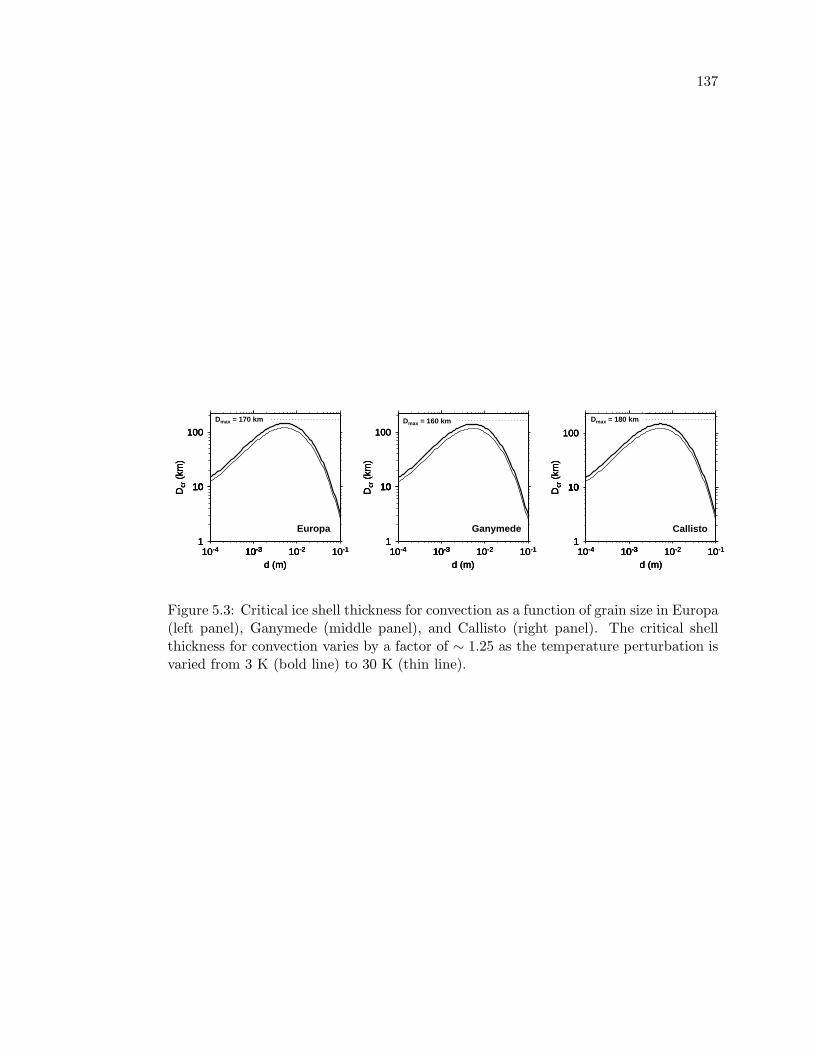
137

1

1010

100

Dcr

(km

)

10-4 10-310-3 10-2 10-1

d (m)

1

1010

100

Dcr

(km

)

10-4 10-310-3 10-2 10-1

d (m)

1

1010

100

Dcr

(km

)

10-4 10-310-3 10-2 10-1

d (m)

Dmax = 170 km

Europa

Dmax = 170 km

1

1010

100

Dcr

(km

)

10-4 10-310-3 10-2 10-1

d (m)

1

1010

100

Dcr

(km

)

10-4 10-310-3 10-2 10-1

d (m)

1

1010

100

Dcr

(km

)

10-4 10-310-3 10-2 10-1

d (m)

Dmax = 170 km

Ganymede

Dmax = 160 km

1

1010

100

Dcr

(km

)10-4 10-310-3 10-2 10-1

d (m)

1

1010

100

Dcr

(km

)10-4 10-310-3 10-2 10-1

d (m)

1

1010

100

Dcr

(km

)10-4 10-310-3 10-2 10-1

d (m)

Dmax = 160 km

Callisto

Dmax = 180 km

Figure 5.3: Critical ice shell thickness for convection as a function of grain size in Europa(left panel), Ganymede (middle panel), and Callisto (right panel). The critical shellthickness for convection varies by a factor of ∼ 1.25 as the temperature perturbation isvaried from 3 K (bold line) to 30 K (thin line).

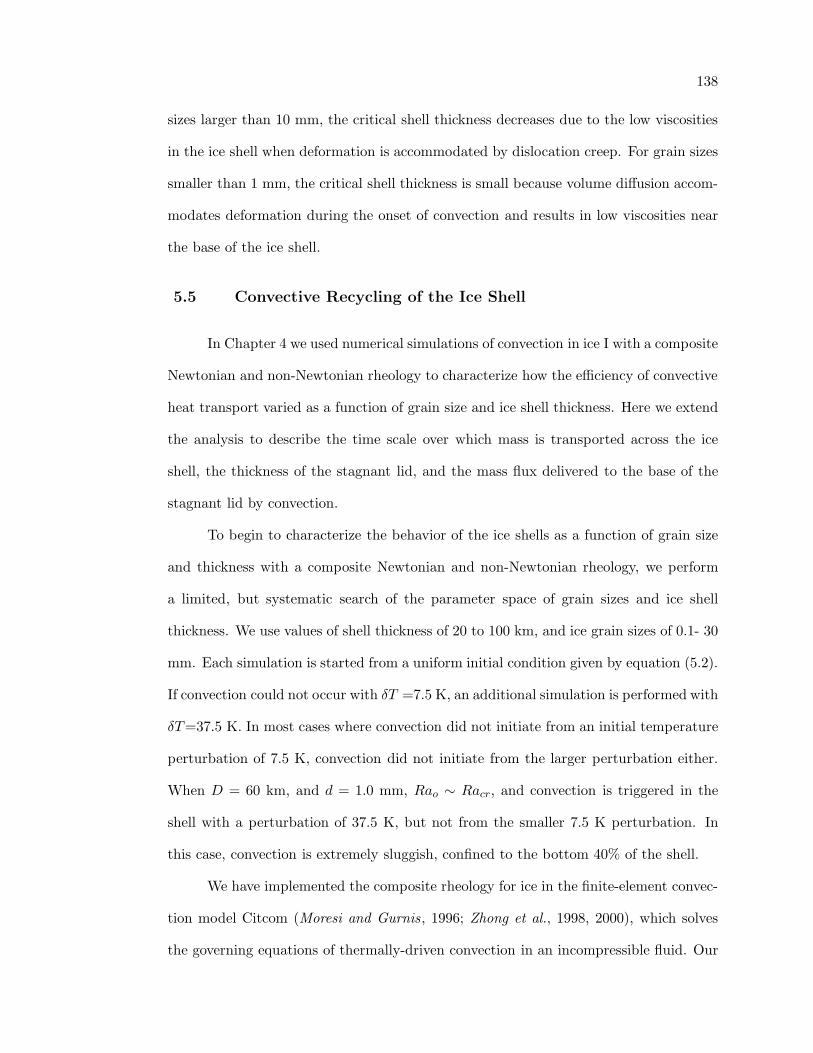
138

sizes larger than 10 mm, the critical shell thickness decreases due to the low viscosities

in the ice shell when deformation is accommodated by dislocation creep. For grain sizes

smaller than 1 mm, the critical shell thickness is small because volume diffusion accom-

modates deformation during the onset of convection and results in low viscosities near

the base of the ice shell.

5.5 Convective Recycling of the Ice Shell

In Chapter 4 we used numerical simulations of convection in ice I with a composite

Newtonian and non-Newtonian rheology to characterize how the efficiency of convective

heat transport varied as a function of grain size and ice shell thickness. Here we extend

the analysis to describe the time scale over which mass is transported across the ice

shell, the thickness of the stagnant lid, and the mass flux delivered to the base of the

stagnant lid by convection.

To begin to characterize the behavior of the ice shells as a function of grain size

and thickness with a composite Newtonian and non-Newtonian rheology, we perform

a limited, but systematic search of the parameter space of grain sizes and ice shell

thickness. We use values of shell thickness of 20 to 100 km, and ice grain sizes of 0.1- 30

mm. Each simulation is started from a uniform initial condition given by equation (5.2).

If convection could not occur with δT =7.5 K, an additional simulation is performed with

δT=37.5 K. In most cases where convection did not initiate from an initial temperature

perturbation of 7.5 K, convection did not initiate from the larger perturbation either.

When D = 60 km, and d = 1.0 mm, Rao ∼ Racr, and convection is triggered in the

shell with a perturbation of 37.5 K, but not from the smaller 7.5 K perturbation. In

this case, convection is extremely sluggish, confined to the bottom 40% of the shell.



the governing equations of thermally-driven convection in an incompressible fluid. Our

139

simulations are run in 2D Cartesian geometry, and free-slip boundary conditions are

used on the surface (z = 0), base (z = −D), and side walls (x = 0, xmax) of the domain.

The simulations used to characterize the convective heat flux and used for analysis

in this section are performed in a domain with 64 x 64 elements, chosen to allow sufficient

numerical resolution across the rheological boundary layer between the stagnant lid and

convecting interior for simulations where Ra ≫ Racr. To ensure numerical stability,

the values of viscosity are not permitted to fall below 10−7ηo or exceed 107ηo. In the

vast majority of cases, the upper limit is reached near the cold surface of the ice shell,

but the lower limit of viscosity is not reached. All simulations are run until the Nusselt

number converges to within 0.01% per time step.

Figure 5.4 illustrates the parameter space explored, and which parameter sets

resulted in convection. The scaling relationship between the critical ice shell thickness

for convection and the grain size of ice (equation 5.4) for δT = 7.5 K is shown for

comparison. For large shell thickness D ≥ 100 km and grain sizes d ≤ 3 mm and d ≥ 30

mm, the effective Rayleigh number of the ice shell is greater than 109, which did not

permit solutions to be found given the numerical resolution used.

5.5.1 Geophysical Descriptive Parameters

Figure 5.5 illustrates the convective temperature field with superimposed velocity

vectors, time evolution of the dimensonless heat flux (Nusselt number, Nu), and plots

of the total viscosity, effective viscosity due to volume diffusion, grain boundary sliding

and basal slip (collectively, grain size-sensitive, or GSS creep), and dislocation creep for

a sample simulation in our study with 0.3 mm in an ice shell 85 km thick. With a small

grain size, deformation in the ice shell is controlled by volume diffusion, which yields

small viscosities in the convecting sub-layer of the ice shell and vigorous convection.

Figure 5.6 shows a similar plot, for convection in ice with a grain size of 30 mm in an ice

shell 85 km thick. For this value of grain size, deformation in the ice shell is controlled

140

largely by dislocation creep, which is highly non-Newtonian. In both cases, convective

motion is confined beneath a stagnant lid which occupies the top 25% of the ice shell,

and the horizontal structure of the flow fields are similar.

The middle panel of Figure 5.7 demonstrates the definition of stagnant lid thick-

ness from the profile of the magnitude of velocity, consistent with the definition of

Solomatov and Moresi (2000). The thickness of the stagnant lid depends on grain size,

and increases as a function of grain size from 0.1 mm - 1 mm as GSS creep is activated

and the ice becomes more viscous. When the grain size of ice is between 3 and 10 mm,

convection does not occur and the entire ice shell remains essentially motionless.

When the grain size is increased to 30 mm, ice shells thinner than 100 km are

able to convect and the thickness of the stagnant lid is of order 30-50% of the shell

thickness. Figure 5.8 illustrates the variation in stagnant lid thickness as a function of

grain size for several values of ice shell thickness.

The left panel of Figure 5.7 illustrates the internal convective temperature based

on the temperature profile in the convecting ice shell, consistent with the definition

of Solomatov and Moresi (2000). The internal convective temperature is given by the

maximum horizontally averaged temperature above the bottom thermal boundary layer.

Beneath the stagnant lid, the ice shell warms to a temperature close to its melting point,

between 250 and 252 K, which is essentially independent of grain size.

The viscosity of the ice shell in the convecting interior is typically of order 1013

Pa s when the grain size of ice is small, 0.1 mm - 0.3 mm and volume diffusion controls

flow. For larger grain sizes the viscosity in the convecting interior is of order 1014 to

1015 Pa s, and convection is sluggish.

5.5.2 Astrobiologically Relevant Parameters

The mass flux of ice delivered to the base of the stagnant lid is calculated from

the mean value of the magnitude of vertical velocity beneath the stagnant lid, (〈vz〉). To

141

20

40

60

80

100

D (

km)

10-410-4 10-3 10-2 10-1

d (m)

20

40

60

80

100

D (

km)

10-410-4 10-3 10-2 10-1

d (m)

20

40

60

80

100

D (

km)

10-410-4 10-3 10-2 10-1

d (m)

20

40

60

80

100

D (

km)

10-410-4 10-3 10-2 10-1

d (m)

Figure 5.4: Parameter space of grain size (d) and ice shell thickness (D) explored in thisstudy. Crosses indicate that convection did occur, triggered from an initial temperatureperturbation of 7.5 K. Filled squares indicate that convection did not occur in the iceshell, even when the temperature perturbation is 37.5 K. When D=60 km and d=10−3

m, Ra ∼ Racr, and convection initiated from a temperature perturbation of 37.5 K, butnot from the smaller 7.5 K perturbation.

142

-80

-60

-40

-20

0

Dep

th (

km)

0 20 40 60 80

X (km)

-80

-60

-40

-20

0

Dep

th (

km)

0 20 40 60 80

X (km)

a)

120

140

160

180

200

220

240

260T (K)

1

2

3

4

Nu

0 50 100

t (Myr)

b)

-80

-60

-40

-20

0

Dep

th (

km)

0 20 40 60 80

X (km)

-80

-60

-40

-20

0

Dep

th (

km)

0 20 40 60 80

X (km)

c)

13141516171819202122

log η (Pa s)

-80

-60

-40

-20

Dep

th (

km)

20 40 60 80

X (km)

-80

-60

-40

-20

Dep

th (

km)

20 40 60 80

X (km)

13141516171819202122

log η (Pa s)d)

-80

-60

-40

-20

Dep

th (

km)

20 40 60 80

X (km)

-80

-60

-40

-20

Dep

th (

km)

20 40 60 80

X (km)

13141516171819202122

log η (Pa s)e)

-80

-60

-40

-20

Dep

th (

km)

20 40 60 80

X (km)

-80

-60

-40

-20

Dep

th (

km)

20 40 60 80

X (km)

13141516171819202122

log η (Pa s)f)

Figure 5.5: Convection in an ice shell 85 km thick with a grain size of 0.3 mm. (a)Convective temperature field with superimposed velocity vectors, (b) time evolution ofthe dimensionless heat flux, or Nusselt number (Nu). (c) The total viscosity, (d) effectiveviscosity due to volume diffusion, (e) GSS creep, and (f) dislocation creep. Convectionis confined beneath a stagnant lid approximately 22 km thick, and the Nusselt numberis 3.03, corresponding to a heat flux of 17.64 mW m−2. Deformation in the ice shellis controlled by volume diffusion, which predicts the smallest viscosities of the fourmechanisms. The effective viscosity due to dislocation creep is much greater than 1022

Pa s, indicating that the contribution to the total strain rate from dislocation creep isnegligible in the ice shell under these conditions. Contours of constant viscosity, whereeach contour line represents a factor of 10 increase in viscosity, are shown for dislocationcreep to illustrate that the viscosity field mirrors the temperature field, even when theviscosity is strongly stress-dependent.

143

-80

-60

-40

-20

0

Dep

th (

km)

0 20 40 60 80

X (km)

-80

-60

-40

-20

0

Dep

th (

km)

0 20 40 60 80

X (km)

a)

120

140

160

180

200

220

240

260T (K)

1

2

3

4

Nu

0 50 100

t (Myr)

b)

-80

-60

-40

-20

0

Dep

th (

km)

0 20 40 60 80

X (km)

-80

-60

-40

-20

0

Dep

th (

km)

0 20 40 60 80

X (km)

c)

13141516171819202122

log η (Pa s)

-80

-60

-40

-20

Dep

th (

km)

20 40 60 80

X (km)

-80

-60

-40

-20

Dep

th (

km)

20 40 60 80

X (km)

13141516171819202122

log η (Pa s)d)

-80

-60

-40

-20

Dep

th (

km)

20 40 60 80

X (km)

-80

-60

-40

-20

Dep

th (

km)

20 40 60 80

X (km)

13141516171819202122

log η (Pa s)e)

-80

-60

-40

-20

Dep

th (

km)

20 40 60 80

X (km)

-80

-60

-40

-20

Dep

th (

km)

20 40 60 80

X (km)

13141516171819202122

log η (Pa s)f)

Figure 5.6: Similar to Figure 5.5, but the grain size of ice is 30 mm. Convection is stillconfined beneath a stagnant lid approximately 22 km thick, but here, deformation iscontrolled by dislocation creep (n = 4), which predicts the smallest viscosities of thefour mechanisms. Slight fluctuations to the total viscosity at the 1% level are introducedby GSS creep. The heat flux across the ice shell is 16.67 mW m−2, corresponding to aNusselt number of 2.88.

144

-60

-45

-30

-15

0

Dep

th (

km)

125 150 175 200 225 250T (K)

-60

-45

-30

-15

0

Dep

th (

km)

125 150 175 200 225 250T (K)

Ti

a)

0.00 0.05 0.10 0.15 0.20 0.25|v| (m/yr)

0.00 0.05 0.10 0.15 0.20 0.25|v| (m/yr)

max(d|v|/dz)

b)

0.00 0.05 0.10 0.15 0.20 0.25|v| (m/yr)

0.00 0.05 0.10 0.15 0.20 0.25|v| (m/yr)

0.00 0.05 0.10 0.15 0.20 0.25|v| (m/yr)

δL

0.00 0.05 0.10 0.15abs(vz) (m/yr)

0.00 0.05 0.10 0.15abs(vz) (m/yr)

0.00 0.05 0.10 0.15abs(vz) (m/yr)

<vz>

<vz>

c)

0.00 0.05 0.10 0.15abs(vz) (m/yr)

(D-δL)

Mass Flux = ρ <vz>(D-δL)2

Figure 5.7: (a) Illustration of the interior convective temperature. (b) Illustration ofthe thickness of the stagnant lid based on its definition from the profile of velocitymagnitude (|v| ≡

√

v2x + v2

z). (c) The mean absolute value of vertical velocity belowthe stagnant lid (〈vz〉) is used to calculate the mass flux at the base of the stagnant lidfrom the convective velocity field.

145

0

25

50

75

δ L (

km) D=85 km

0

25

50

75

δ L (

km)

0

25

50

75

δ L (

km)

No Convection

0

25

50

75

δ L (

km) D=75 km

0

25

50

75

δ L (

km)

0

25

50

75

δ L (

km)

No Convection

0

25

50

δ L (

km) D=60 km

0

25

50

δ L (

km)

0

25

50

δ L (

km)

No Convection

0

25

δ L (

km)

10-410-4 10-3 10-2 10-1

d (m)

D=35 km

0

25

δ L (

km)

10-410-4 10-3 10-2 10-1

d (m)

0

25

δ L (

km)

10-410-4 10-3 10-2 10-1

d (m)

No Convection

Figure 5.8: Variation in the thickness of the stagnant lid (δL) with grain size of ice(d). For grain sizes less than 3.0 mm, as the grain size of ice is increased, GSS creep isactivated, causing the ice to stiffen, resulting in sluggish convection and an increase instagnant lid thickness with grain size. For intermediate grain sizes 3 − 10 mm, the iceis too stiff to convect. When dislocation creep is activated in ice with a grain size of 30mm, convection can occur, resulting in a relatively thin stagnant lid.

146

calculate the mass flux, we average the absolute value of the vertical velocity (abs(vz))

beneath the stagnant lid and multiply by the density of ice and thickness of the con-

vecting sub-layer to obtain a mass flux,

M = ρ〈vz〉(D − δL)2, (5.6)

where by multiplying by (D− δL)2 we have implicitly assumed that the structure of the

flow field in the third unused y dimension is the same as the x dimension. The right

panel of Figure 5.7 demonstrates the definition of the mass flux. Figure 5.9 illustrates

the variation in mass flux as a function of grain size for various values of shell thickness.

When convection does not occur, the mass flux is zero.

When convection occurs, the mass flux delivered to the base of the stagnant lid

is of order 109 to 1013 kg yr−1, and is strongly dependent on the grain size of ice, which

controls the vigor of convection. Assuming 1 cell cm−3, as estimated by Chyba and

Phillips (2002) is sustained in Europa’s ocean due to equilibration of surface ices, and

the efficiency of entrainment of oceanic microbes in the ice shell is 100%, 1021 to 1025

cell yr−1 could be delivered to the base of the stagnant lid each year, where endogenic

resurfacing events would be required to deliver them to the surface.

The time scale to recycle the convecting sub layer of the ice shell can be calculated

from the mean vertical velocity,

τrecyc =(D − δL)

〈vz〉. (5.7)

Figure 5.10 illustrates the variation in recycling time scale as a function of grain size for

a variety of ice shell thicknesses. When convection does not occur, the recycling time

scale for the ice shell is essentially infinite, and is not displayed on the plot.

When convection occurs, cycling of the material beneath the stagnant lid within

the ice shell is fast, and occurs on time scales less than the 107 yr surface age of Europa.

The recycling time scales are 105 to 107 yr, which indicates that sufficient chemical

147

109

10101010

1011

1012

1013

M (

kg y

r-1)

109

10101010

1011

1012

1013

M (

kg y

r-1)

109

10101010

1011

1012

1013

M (

kg y

r-1) D=85 km

No Convection

109

10101010

1011

1012

1013M

(kg

yr-1

)

109

10101010

1011

1012

1013M

(kg

yr-1

)

109

10101010

1011

1012

1013M

(kg

yr-1

) D=75 km

No Convection

109

10101010

1011

1012

1013

M (

kg y

r-1)

109

10101010

1011

1012

1013

M (

kg y

r-1)

109

10101010

1011

1012

1013

M (

kg y

r-1) D=60 km

No Convection

109

10101010

1011

1012

1013

M (

kg y

r-1)

10-410-4 10-3 10-2 10-1

d (m)

109

10101010

1011

1012

1013

M (

kg y

r-1)

10-410-4 10-3 10-2 10-1

d (m)

109

10101010

1011

1012

1013

M (

kg y

r-1)

10-410-4 10-3 10-2 10-1

d (m)

D=35 km

No Convection

Figure 5.9: Mass flux of ice delivered to the base of the stagnant lid through convectivecirculation as a function of grain size of ice, for ice shell thicknesses from 85 km (toppanel) to 35 km (bottom panel). The mass fluxes are of order 109 to 1013 kg yr−1. Whenconvection does not occur, the mass flux is zero and is not displayed on the graph.

148

105

106106

107

τ rec

yc (

yr)

105

106106

107

τ rec

yc (

yr)

105

106106

107

τ rec

yc (

yr) D=85 km

No Convection

105

106106

107τ r

ecyc

(yr

)

105

106106

107τ r

ecyc

(yr

)

105

106106

107τ r

ecyc

(yr

) D=75 km

No Convection

105

106106

107

τ rec

yc (

yr)

105

106106

107

τ rec

yc (

yr)

105

106106

107

τ rec

yc (

yr) D=60 km

No Convection

105

106106

107

τ rec

yc (

yr)

10-410-4 10-3 10-2 10-1

d (m)

105

106106

107

τ rec

yc (

yr)

10-410-4 10-3 10-2 10-1

d (m)

105

106106

107

τ rec

yc (

yr)

10-410-4 10-3 10-2 10-1

d (m)

No Convection

D=35 km

Figure 5.10: Time scale (τrecyc) to recycle the convecting sublayer of the ice shell definedin equation (5.7). The recycling time scales are of order 105 to 107 years, however,resurfacing events are likely required to permit exchange of materials across the stagnantlid.

149

energy can be delivered to the ocean to permit the possibility of a biosphere powered by

decay of 40K, which is generated within the ice shell and can be delivered by convection

alone. The thick stagnant lid present at the surface of the ice shell prevents convective

motions from reaching the surface, so a biosphere powered by radiation products from

the surface of Europa, requires resurfacing events to breach the stagnant lid. Resurfacing

events are also required to deliver microbes or interesting ocean chemistry directly to

the surfaces of the satellites.

5.6 Endogenic Resurfacing Events on Europa

Regardless of which deformation mechanism acommodates convective strain in

the ice shell, the viscosity of ice is strongly temperature dependent, leading to the

formation of a thick stagnant lid of cold ice near the surface of the ice shell. However,

the presence of abundant endogenic resurfacing on Europa and Ganymede suggests that

convective motions can breach the stagnant lid.

Here we discuss two methods of surface/sub-surface exchange that could enable

material from the convecting zone to reach the relatively shallow subsurface where

ocean chemistry and potentially, microbial life, could be sampled by a lander, or permit

radiation products from the surface to reach the convecting sub-layer. We focus on

the role of extrusive domes on Europa and the formation of double ridges, which are

features that have been addressed in studies performed in conjunction with this thesis.

5.6.1 Domes

A large number of circular and quasi-circular pits, spots, and domes, collectively

referred to as “lenticulae,” have been observed on Europa. The sizes of these features

range from 1-10’s of km with a mean diameter of ∼ 7 km (Spaun, 2001), and uplifts

of order 100 m. Based on their morphologies and similarity in size and spacing, it has

been suggested that they form due to thermal convection in an ice shell 10’s of km thick

150

(Pappalardo et al., 1998). Dynamic topography from our convection models appropriate

for Europa’s ice shell indicate that uplifts due to thermal convection alone are of order 10

m (Figure 5.11), consistent with results from Newtonian convection models (Showman

and Han, 2004).

Domes on Europa may represent diapiric upwellings of relatively salt-free ice in a

water ice plus hydrated salt ice shell, where compositional and thermal buoyancy act in

concert to form uplifts of 100’s of meters with percentage-level differences in composition

(Pappalardo and Barr , 2004). Density differences due to compositional variations in

the ice shell that drive diapiric rise can easily exceed the density differences due to

thermal buoyancy. The maximum convective stress in the ice shell is (McKinnon, 1998;

Pappalardo and Barr , 2004):

σmax ∼ 0.1ρigα∆TD (5.8)

where ρi is the density of pure water ice. The maximum thermal available to drive

thermal convection is

∆ρconv ∼ 0.1ρiα∆T, (5.9)

which is approximately 1.4 kg m−3 if the density of ice is 930 kg m−3. The density

difference between salt-free ice and ice doped with salt is

∆ρcompositional ∼ φ(ρle − ρi) (5.10)

where φ is the volume fraction of low-eutectic salts that will melt out of the ice shell

upon heating, and ρle is the density of the low-eutectic salt (Pappalardo and Barr ,

2004). The density difference due to compositional variations in the ice shell will exceed

the density difference due to thermal expansion when

φ >0.1ρiα∆T

(ρle − ρi). (5.11)

If the density of the low-eutectic salts is 1500 kg m−3 (Pappalardo and Barr , 2004),

compositional buoyancy dominates over thermal buoyancy for φ > 0.003. Therefore,

151

-50

-25

0

25

50

h top

o (m

)

-50

-25

0

25

50

h top

o (m

)

-50

-25

0

25

50

h top

o (m

)

-50

-25

0

25

50

h top

o (m

)

-50

-25

0

25

50

h top

o (m

)

-50

-25

0

25

50

h top

o (m

)

D=85 km D=75 km

-50

-25

0

25

50

h top

o (m

)

10-410-4 10-3 10-2 10-1

d (m)

-50

-25

0

25

50

h top

o (m

)

10-410-4 10-3 10-2 10-1

d (m)

-50

-25

0

25

50

h top

o (m

)

10-410-4 10-3 10-2 10-1

d (m)

-50

-25

0

25

50

h top

o (m

)

10-410-4 10-3 10-2 10-1

d (m)

-50

-25

0

25

50

h top

o (m

)

10-410-4 10-3 10-2 10-1

d (m)

-50

-25

0

25

50

h top

o (m

)

10-410-4 10-3 10-2 10-1

d (m)

-50

-25

0

25

50

h top

o (m

)

10-410-4 10-3 10-2 10-1

d (m)

-50

-25

0

25

50

h top

o (m

)

10-410-4 10-3 10-2 10-1

d (m)

D=60 km

10-410-4 10-3 10-2 10-1

d (m)10-410-4 10-3 10-2 10-1

d (m)10-410-4 10-3 10-2 10-1

d (m)10-410-4 10-3 10-2 10-1

d (m)10-410-4 10-3 10-2 10-1

d (m)10-410-4 10-3 10-2 10-1

d (m)

D=35 km

Figure 5.11: Dynamic topography from convection on Europa for D = 85 km (top, left),D = 75 km (top, right), D = 60 km (bottom, left) and D = 35 km (bottom, right).Filled squares indicate the maximum and minimum topography in meters. The surfaceof the convecting layer is drawn down by up to 50 meters, and upwellings are limitedto 10’s of meters.

152

a difference in volumetric salt content > 0.3 % can provide more driving stress for

the formation of domes on Europa than thermal buoyancy. Driven by compositional

buoyancy, diapirs responsible for dome formation may be able to extrude onto the

surface of Europa, or in some cases stall in the shallow subsurface to form an uplifted

plateau.

The approximate volume of ice erupted onto the surface during a dome formation

event is approximately πr2h ∼ 3×1015 cm 3 for a dome with a radius of 3.5 km and height

of 100 m. If the material contained in the dome is transported directly from the ocean

without dilution, up to 3×1015 cells (assuming the concentration of microbes predicted

by Chyba and Phillips (2002)) or 3 × 1021 cells (assuming the microbe concentration

predicted by Chyba and Hand (2001)) could be contained within the erupted diapir

head. Detecting such microbes would require drilling to a depth of greater than 1

meter, beneath the layer of surface ice that has been chemically modified by particles

and radiation.

5.6.2 Ridges

The most common features on Europa’s surface are double ridges, which consist of

ridge pairs each separated by a central trough (Greeley et al., 1998). Ridges are typically

a few kilometers wide and up to several hundred kilometers long; many exhibit signs

of strike-slip faulting with offsets of ∼ 1 to 10 km (Hoppa et al., 1999). One proposed

method of ridge formation suggests that double ridges form in response to frictional

heating of the ice crust as fault blocks slide past one another in response to tidal flexing

of the shell (Nimmo and Gaidos, 2002). Friction between the moving fault blocks causes

localized heating due to viscous dissipation along the fault plane, local thinning of the

brittle lithosphere, and thermally driven upwelling, which may form the uplifted ridge

structure (Nimmo and Gaidos, 2002). If melting occurs along the fault zone and can

drain vertically into the convecting portion of the ice shell, it could become incorporated

153

into a convective downwelling and potentially drain to the ocean, providing a means by

which surface material could be buried on geologically short time scales (Barr et al.,

2002).

5.7 Ocean Stability

The results of Chapter 4 indicate that when convection occurs, efficient convective

heat transfer across the shell can lead to freezing of the internal oceans in the satellites.

When convection occurs, the ice shells thicken by meters per year, which over geological

time scales can cause the vigor of convection to increase, leading to runaway freezing of

the ocean. Furthermore, the present heat flux from radiogenic heating in the interiors

of a Ganymede- and Callisto-like satellite cannot provide enough heat to maintain an

internal liquid water ocean in the absence of tidal heating, even if the ice shell cannot

convect. Oceans are marginally stable beneath non-convecting ice shells 1.5 billion years

ago when radiogenic heat fluxes were twice their present values. Tidal dissipation may

play a role in providing additional heat to the ice shells to offset efficient heat transport

by convection, however, the details of the interaction between tidal dissipation and

convection are not well-constrained. The presence of liquid water oceans in Callisto

today suggests that some non-water-ice material is present to depress the freezing point

of the ice shell. The presence of a liquid water ocean in Ganymede at present suggests

that the freezing point of the shell is depressed, or that remnant energy from passage

through a tidal resonance or cooling of Ganymede’s core is maintaining the ocean at

present. Therefore, even if the oceans of the satellites are habitable, tidal flexing of the

ice shells or non-water-ice materials may be required to prevent the oceans from freezing

and permit biological activity.

154

5.8 Summary

Under what conditions can convection occur? The critical ice shell thickness for

convection is a strong function of the grain size of ice and the amplitude and wavelength

of temperature perturbation issued to the ice shell. For small grain sizes (d < 1 mm)

the critical shell thickness for convection is < 30 km, because convective strain is ac-

commodated by volume diffusion and the viscosity at the base of the ice shell is small.

For large grain sizes (d > 10 mm), the critical shell thickness for convection is also

small, because strain is accommodated by dislocation creep, permitting low viscosities

at the base of the ice shell. For intermediate grain sizes, the critical shell thickness for

convection maximizes at 130 km.

When convection occurs, the stagnant lid thickness, convective heat flux, and

vigor of the convection are critically dependent on the grain size of ice. When convection

occurs, it provides swift and efficient recycling of the material beneath the stagnant lid.

The mass flux of ice delivered to the base of the stagnant lid is of order 109 - 1013 kg

yr−1, and the time scale for recycling of ice between the base of the shell and the base

of the stagnant lid is of order 105 to 107 yr.

However, resurfacing events are required to breach the stagnant lid to bring po-

tential microbes to the relatively shallow subsurface where they might be detected by

landed spacecraft. We view domes and double ridges on Europa as potential sites where

interesting ocean chemistry may be entrained in the shallow subsurface, either directly,

by extrusive cryovolcanism, or indirectly through passive thermal uplift.

Chapter 6

Conclusions and Future Work

6.1 Answers to the Key Questions

In this thesis, the following questions have been addressed:

What are the conditions required to initiate convection in an initially

conductive ice I shell with a non-Newtonian rheology?

The convective stability of a non-Newtonian ice shell can be judged by comparing

the Rayleigh number of the shell to a critical value. Previous studies suggest that the

critical Rayleigh number for a non-Newtonian fluid depends on the initial conditions

in the fluid layer, in addition to the thermal, rheological, and physical properties of

the fluid. We seek to extend the existing definition of the critical Rayleigh number

for a non-Newtonian, basally heated fluid by quantifying the conditions required to

initiate convection in an ice I layer initially in conductive equilibrium. The critical

Rayleigh number for the onset of convection in ice I varies as a power (-0.6 to -0.5)

of the amplitude of the initial temperature perturbation issued to the layer, when the

amplitude of perturbation is less than the rheological temperature scale. For larger

amplitude perturbations, the critical Rayleigh number achieves a constant value. The

critical Rayleigh number is characterized as a function of surface temperature of the

satellite, melting temperature of ice, and rheological parameters so that the results

presented here may be extrapolated for use with other rheologies and for a generic large

icy satellite. The values of critical Rayleigh number imply that triggering convection

156

from a conductive equilibrium in a pure ice shell less than 100 km thick in Europa,

Ganymede, or Callisto requires a large, localized temperature perturbation of 1-10’s K

to soften the ice, and therefore may require tidal dissipation in the ice shell.

How do the conditions required to trigger convection in an ice I shell

change if a composite Newtonian and non-Newtonian rheology for ice I is

used?

When a composite Newtonian and non-Newtonian rheology for ice I is used, the

critical Rayleigh number for convection varies as a power (−0.2) of the amplitude of ini-

tial temperature perturbation, for perturbation amplitudes between 3 K and 30 K. The

critical Rayleigh number depends strongly on the grain size of ice, which governs the

transition stresses between the Newtonian and non-Newtonian deformation mechanisms.

The critical ice shell thickness for convection in all three satellites is < 30 km if the ice

grain size is <1 mm. In this case, the relatively low thermal stresses associated with

plume growth are not sufficient to activate weakly non-Newtonian grain-size-sensitive

(GSS) creep, so plume growth is controlled by Newtonian volume diffusion. The critical

shell thickness is <30 km for grain sizes >1 cm, where thermal stresses can activate

strongly non-Newtonian dislocation creep, and the ice softens as it flows. For interme-

diate grain sizes (1-10 mm), weakly non-Newtonian grain-size-sensitive creep controls

plume growth, yielding critical shell thicknesses close to the maximum permitted shell

thickness for each of the Galilean satellites. Regardless of the rheology that controls

initial plume growth, a finite amplitude temperature perturbation is required to soften

the ice to permit convection, and this may require tidal dissipation.

Given a composite rheology for ice I, are oceans beneath a layer of

ice I thermodynamically stable against heat transport by convection and

conduction?

Basally heated shells 20 - 100 km thick with assumed uniform grain size of ≤ 0.3

mm convect vigorously with heat fluxes between 30-40 mW m−2 because Newtonian

157

volume diffusion accommodates convective strain and results in low ice viscosities in

the convecting sub-layer. If the ice has a grain size ≥ 30 mm, dislocation creep accom-

modates strain, convection is sluggish, and convective heat fluxes are 15 - 20 mW m−2.

When convection occurs in the absence of tidal dissipation, the heat flux across an ice

shell can exceed the radiogenic heat flux, casuing the ice shell to thicken by meters per

year. If the ice shell has a grain size of 3-10 mm, it cannot convect if < 100 km thick,

permitting internal oceans to be thermodynamically stable in a Ganymede/Callisto-like

satellite in the absence of tidal dissipation or non-water-ice materials, given chondritic

heating rates appropriate for 1.5 billion years ago. If the melting point of the ice shell

is depressed due to the presence of non-water-ice materials such as sulfuric acid hydrate

or ammonia, oceans may be stable beneath conductive ice shells. If tidal dissipation

occurs in the ice I shell, additional heat may be supplied to balance efficient heat trans-

port, and may permit oceans to be thermodynamically stable. If tidal dissipation is

capable of changing the mode of heat transport across the ice I shell, the tidal and

convective/conductive heat fluxes are linked quantities. More detailed modeling of tidal

dissipation is necessary to clarify how tidal heat is spatially localized in the ice shell,

and to investigate whether a feedback between tidal heating and convection occurs.

Does convection play a role in enhancing the habitability of the internal

oceans of the icy satellites?

If convection occurs in an ice I layer, fluid motions are confined beneath a thick

lid of immobile ice, approximately 30 to 50% of the thickness of the ice shell. The

thickness of the stagnant lid is dependent on the grain size of ice. Convective motions

deliver 109 to 1013 kg yr−1 of ice to the base of the stagnant lid where resurfacing events

such as the formation of domes or ridges on Europa may deliver the ice onto the surface.

Triggering convection in an initially conductive ice I shell requires modest amplitude (a

few to 10’s K) temperature anomalies to soften the ice to permit convection, which may

require tidal dissipation. Therefore, tidal and compositional effects may be required to

158

permit communication between the surfaces and oceans of the satellites.

6.2 Future Work

6.2.1 Grain Size Evolution

Conclusions regarding the convective stability and heat flux of the ice shells drawn

from this study are strongly dependent on the grain size of ice. A uniform grain size has

been assumed in all models of the ice shells presented in this thesis. However, the grain

size of ice in the shells of the satellites likely changes as a function of depth, temperature,

total accumulated convective strain, strain rate, and impurity content in the ice shell.

By analogy with terrestrial ice sheets, ice shelves, and the Earth’s mantle, a

complex suite of processes is likely to occur within the ice shells of the satellites to

cause grain sizes to evolve as the temperature and velocity field in the shells change.

If grain growth or destruction occurs in ice, the change in grain size may cause the

controlling deformation mechanism to change, changing the rheology of ice.

Flow by certain microphysical deformation mechanisms may cause the grain size

of the ice to change. For example, flow by dislocation creep is likely to lead to smaller

grain sizes, whereas flow by grain boundary sliding or diffusional flow is likely to lead

to grain growth (e.g. De Bresser, et al., 1998). Based on laboratory observations

using a metallic rock analog that deforms by diffusional flow and dislocation creep, De

Bresser et al. (1998) argue for a scenario wherein the grains of the material dynamically

recrystallize as the material strains. At each temperature and stress, the material has

a grain size such that the strain rates from dislocation creep and diffusional flow are

equal. A similar effect could be occurring in ice, wherein the grain size dynamically

evolves such that the strain rates from GSS creep and dislocation creep are equal. The

grain size that results in equal strain rates from each mechanism would depend on the

temperature of the ice, and would increase as the temperature decreased.

159

In future modeling efforts, the initial conditions in the ice shell, the evolution of

grain size and grain orientation, and the role of tidal flexing of the ice shell (McKinnon,

1999), and heating by tidal dissipation in changing the grain size of ice will factor into

the behavior of the ice shell, both at the onset of convection, and in convecting ice

shells. Therefore, we advocate using a more realistic grain size model in future work,

by allowing grain size to evolve dynamically as the ice flows.

6.2.2 Tidal Dissipation

Although estimates of the tidal dissipation rates exist for the Galilean satellites,

the details of how tidal dissipation occurs and where it is concentrated within the

satellites are unknown. The role that tidal heating may play in modifying the behavior

of the ice I shells depends on the rheology of ice and a detailed description of the physical

processes responsible for tidal dissipation.

Tidal dissipation could modify the mode of heat transport within the outer ice

I shells of the satellites, by potentially triggering convection in an initially motionless

conductive shell, or squelching convection by generating heat fluxes in excess of the

maximum convective heat flux, resulting in melting at the base of the ice shell. If tidal

heating changes the mode of heat transport in the ice shells, a detailed description of

tidal dissipation must be included in any study of the thermodynamic stability of oceans

in tidally heated satellites. Although the details of tidal heating are not known, some

insight into how tidal dissipation may change the behavior of the ice shells can be gained

by estimating the total amount of heat that may be deposited in the ice shells satellites.

Tidal dissipation must be horizontally localized on length scales similar to λcr ∼

1.75D to generate initial temperature perturbations capable of triggering convection in

the ice I shells of the Galilean satellites. Several models of tidal dissipation in the ice

shell of Europa have been proposed in the literature, each of which predicts a different

spatial pattern of tidal dissipation in the ice shell. The likelihood that tidal dissipation

160

will become spatially localized in the ice shell to generate temperature perturbations to

the ice shell similar to the perturbations used in Chapters 2 through 4 is discussed here.

Tidal effects on the Galilean satellites have endured over geologically long time

scales due to the Laplace resonance between Io, Europa, and Ganymede. Secular per-

turbations on the system due to the resonance among the satellites causes the forced

component of their orbital eccentricities to be replenished on a time scale much shorter

than the eccentricity damping time scale. The persistent non-zero orbital eccentricities

of the satellites results in ongoing dissipation of orbital energy in their interiors, which

undoubtedly drives volcanism on Io (Peale et al., 1979), and may play a role in forming

the interesting geology on the surfaces of Europa and Ganymede discussed in Chapter

1.

As discussed in Chapters 1 and 4, the rate of energy dissipation within a satellite

in eccentric orbit around Jupiter is given by (Peale and Cassen, 1978):

E =21

2

k

Q

R5sGM2

Jne2

a6, (6.1)

where k is the Love number describing the response of satellite’s gravitational to the

applied tidal potential, Rs is the radius of the satellite, G is the gravitational constant,

MJ is the mass of Jupiter, n is the satellite’s mean motion, e is the orbital eccentricity,

Q is the tidal quality factor describing the fractional orbital energy dissipated per cycle,

and a is the semi-major axis of the satellite’s orbit about Jupiter.

The strong 1/a6 dependence in equation (6.1) indicates that dissipation of energy

in the Galilean satellite system will be highest in Io, which is closest to Jupiter, and

the amount of energy dissipation in Europa and Ganymede will be smaller. Also, the

eccentricity of the satellite’s orbit appears as e2, so increasing the eccentricity of the

satellite’s orbit can have profound effects on the thermal state of its interior. In the case

of Ganymede, a tenfold increase in its orbital eccentricity can cause widespread melting

in the interior provided kQ changes on a longer time scale (Showman and Malhotra,

161

1997).

The value of Love number k and the tidal quality factor Q are shorthand for

a tremendous amount of physics that describes the deformation occurring within a

viscoelastic satellite in response to the applied tidal force. An upper bound on k of 0.25

can be obtained assuming the satellite has an essentially zero rigidity, and exhibits a

hydrostatic response to the applied tidal potential. A satellite with a thin floating ice

shell might exhibit such a response (Moore and Schubert , 2000). If the satellite does

not have an internal ocean, and the ice I layer is rigidly coupled to the rock or ice

layers within the satellite, k becomes very small. For example, if Ganymede does not

have an ocean, k ∼ 0.02 (Murray and Dermott , 1999). Because the tidal dissipation is

proportional to k, and k ∼ 0 for a satellite without an internal water ocean, it is likely

that tidal dissipation in an icy satellite can only help to maintain an ocean, not create

an ocean.

The tidal quality factor, Q, expresses the fractional energy dissipated per cycle:

Q =2πEo∮

Edt(6.2)

where Eo is the orbital energy of the satellite. Values of the tidal quality factor are

not well constrained for any satellite in the solar system other than Earth’s moon, but

Q ∼ 100 is commonly assumed for the icy satellites (Murray and Dermott, 1999 and

references therein.) The value of Q for the satellite depends on the amount of non-

recoverable viscous deformation that occurs within the satellite over a single orbital

cycle. For a viscoelastic satellite, the Love number k is complex, and the amount of

energy lost per cycle is proportional to the imaginary part of k (Segatz et al., 1988):

E =21

2Im(k)

(nRs)5

Ge2. (6.3)

In the Galilean satellites, tidal dissipation serves as an important heat source in the

outer ice shells because the viscosity of ice I near its melting point is potentially small

162

enough to permit a significant amount of non-recoverable viscous deformation in the ice

shell over each orbital cycle of the satellite. The value of Im(k) will depend critically

on the rheology of the ice shell. Because the viscosity of the ice is strongly temperature-

dependent, the overall temperature structure of the ice shell could affect the value

Im(k). A thick convecting ice shell with a convective sub-layer warmed to near its

melting point could be a more dissipative state than a cold conductive ice I shell. In a

convective shell, the sub-layer of the shell could undergo appreciable viscous deformation

due to tidal flexing of the shell over a single orbital cycle, causing the total amount of

tidal dissipation could increase. In this way, the heat flux across the ice shell (Fc), which

depends on whether convection occurs or not, and the tidal heat flux (Ftidal) are linked

quantities.

Simple estimates of the rate of energy dissipation given assumed values of k and

Q can shed some light on the role that tidal dissipation might play in modifying the

behavior of the outer ice I shells of the satellites. Energy dissipation rates can be

compared to estimates of the radiogenic heating from the interiors of the satellites to

gain insight into the relative importance of tidal and radiogenic heating in their interior

evolution.

The surface heat flux from tidal dissipation is given by:

Ftidal =E

4πR2s

=21

8π

R3sGM2

Jne2

a6(6.4)

Using k ∼ 0.25 and Q ∼ 100, the surface heat flux from tidal dissipation at present

in Ganymede given its present eccentricity of 0.0015 (Murray and Dermott , 1999) is

approximately 0.15 mW m−2, a factor of 20 less than radiogenic heat fluxes at present,

and a factor of 50 less than radiogenic heat fluxes 1.5 billion years ago (see Table 4.2).

However, if Ganymede experienced a period of increased orbital eccentricity dur-

ing passage through resonances with Europa and Io, e ∼ 0.01, assuming a Q for Jupiter

of 3 × 105 (Showman and Malhotra, 1997). During this time, the surface heat flux due

163

to tidal dissipation would have been 6.75 mW m−2, comparable to the chondritic heat

flux appropriate for 1.5 billion years ago. Using values of k ∼ 0.25, Q ∼ 100, and

e ∼ 0.01 for Europa, (see Table 4.2), its surface heat flux due to tidal dissipation is

approximately 50 mW m−2, a factor of 10 larger than the present chondritic heat flux

of ∼ 5 mW m−2 (Spohn and Schubert , 2003).

If an ice shell is convecting, and tidal dissipation begins to warm its interior, it is

not known whether an equilibrium between dissipation in the ice shell and the convective

heat flux exists. If the tidal heat flux is greater than the maximum convective heat flux,

which is determined by the rheology of the ice, the ice shell will thin and convection will

cease. If the tidal heat flux is less than the convective heat flux the ice shell will thicken.

If the ice shell is thick, but conductive initially, and tidal heating may be able to trigger

convection in the shell, then the evolution of the ice shell and ocean will depend on the

existence of an equilibrium between tidal heating and the convective heat flux.

The rate of energy dissipation defined by equation (6.1) represents a global total

and does not describe how tidal dissipation actually occurs, or where it takes place

within the satellites. To effectively trigger convection in the satellites in the manner

described in Chapters 2 and 3, tidal dissipation must be capable of generating tempera-

ture perturbations on horizontal length scales ∼ λcr. If tidal dissipation is concentrated

on horizontal length scales much larger thanλcr, the critical Rayleigh number would

increase. The critical Rayleigh number for convection under the composite rheology de-

scribed in Chapter 3 is only weakly dependent on the wavelength of initial perturbation,

varying by only 5% for 1.2D < λ < 2.2D. Unfortunately, direct extrapolation of the

Racr(λ) curves from Chapter 3 to wavelengths of 2400 km (∼ 25D to ∼ 100D) can not

yield useful constraints on the critical Rayleigh number for λ ≫ λcr. By analogy with

the shape of the stability curve for an isoviscous fluid (Turcotte and Schubert , 1982), and

for a single non-Newtonian rheology calculated in Chapter 2, the slope of the stability

curve for λ ≫ λcr cannot be assumed to be the same as the slope for λ ∼ λcr. Therefore,

164

the applicability of the Racr values calculated in this thesis to tidally-triggered convec-

tion are dependent upon whether tidal dissipation can become localized on horizontal

length scales ∼ λcr.

Tidal dissipation results from the rapid tidal flexing of the inner three Galilean

satellites. In an ice shell with a laterally homogeneous viscosity structure (i.e. the

ice shell is in conductive equilibrium everywhere), the rapid deformation caused by

the tidal flexing of the ice shell is distributed on relatively long wavelengths λtidal ∼

2πREuropa/4 ∼ 2400 km (Ojakangas and Stevenson, 1989). Several methods have been

recently proposed to localize tidal dissipation in an ice shell. Each model makes a

different prediction about the distribution of tidal dissipation in the ice shell.

The landmark study of Ojakangas and Stevenson (1989) sought to determine the

equilibrium thickness of Europa’s ice shell by equating the heat flux due to tidal dissi-

pation within the ice shell to the conductive heat flux. In this model, tidal dissipation

is expressed by a volumetric dissipation rate that depends on the strain rate of the ice

shell and the Maxwell quality factor, which is explicitly evaluated as a function of the

temperature-dependent viscosity and rigidity of the ice shell. The volumetric dissipation

rate within the ice shell is:

q =2µ〈εij〉

ω

ωτM

1 + (ωτM )2(6.5)

for a Newtonian rheology, where ω = 2π/TEuropa. The time averaged tidal strain rate

(〈εij〉) is evaluated as a function of latitude and longitude at every location on Europa.

The quantity τM = η/µ is the Maxwell time, expressed by the ratio of the viscosity

of the ice to the rigidity of ice. Because the viscosity of ice is strongly temperature-

dependent, the volumetric dissipation rate is a strong function of temperature. The

ice shell is assumed to be thin compared to the radius of the satellite and to behave

as a largely elastic body over the time scale of the tidal forcing. As a result, the tidal

strain rate within the ice shell is assumed to be constant as a function of depth, so tidal

165

dissipation is localized as a function of temperature only. In a conductive ice shell, the

dissipation is therefore a function of depth, and is constant as a function of horizontal

coordinate. On Europa, the maximum dissipation occurs near the melting point of ice I

for reasonable values of melting point viscosity (∼ 1013 − 1015 Pa s) and shear modulus

(µ ∼ 1010Pa). Therefore, the layer of maximum dissipation is likely to be near the base

of the shell, where T ∼ Tm, and is not horizontally localized.

The Ojakangas and Stevenson (1989) model is 1-dimensional, so lateral heat flow

by convection and conduction and potential variations in the tidal strain rate due to

viscosity heterogeneities in the ice shell are not considered. Therefore, interactions

between the geometry of the temperature field within the ice shell and the tidal forcing

function are not considered.

Recent calculations by Tobie et al. (2003) and Showman and Han (2004) imple-

ment a heat source similar to equation (6.5) in 2D Cartesian convection simulations to

provide some intuition as to how convection and tidal dissipation might interact. The

specific form of volumetric heating rate used in these studies is:

H(T ) =Ho

η(T )ηo

+ ηo

η(T )

(6.6)

where ηo is a reference viscosity evaluated at a reference temperature To, chosen so

that τMaxwell ∼ τEuropa (Wang and Stevenson, 2000; Tobie et al., 2003; Showman and

Han, 2004; Tobie et al., 2004). In this formulation, tidal heating is concentrated as

a strong function of the 2-dimensional, heterogeneous temperature field. The extent

to which the tidal heating pattern mirrors the temperature distribution is controlled

by the activation energy in the ice flow law. Such heat sources are currently used

only in Newtonian convection models, because the form of H(T ) comes from equation

(6.5), which is based on a Newtonian rheology for ice (Ojakangas and Stevenson, 1989;

Wang and Stevenson, 2000). The value of Ho is used to scale the total amount of heat

dissipated in the ice shell, and is calculated by different methods in each study that

166

employs such a heat source. As convection begins in an ice shell with internal heating

distributed according to equation (6.6), the base of the ice shell warms to near its

melting point, and the total amount of tidal dissipation in the ice shell increases. If Ho

is small, tidal dissipation does not substantially modify the behavior of the convecting

ice shell. If Ho is large, the heat generated in the ice shell exceeds the heat transported

by convection, and the ice shell melts.

Whether equation (6.6) is applicable to tidal dissipation in an ice I shell with

a highly heterogeneous viscosity structure is not known, and is a matter of debate

in the icy satellites community. Although equation (6.6) may provide a reasonable

approximation of the behavior tidally-heated convection, some have argued that it over-

simplifies the complex interaction between tidal forcing and an ice shell with a highly

heterogeneous viscosity field (Moore, 2001). If the tidal strain rate is uniform over

horizontal spatial scales similar to the width of a convective upwelling, tidal heating

should perhaps be a function of depth only. However, if viscosity heterogeneities in the

ice shell are capable of localizing tidal strain, tidal dissipation may become localized in

low viscosity zones in the ice shell.

The volumetric dissipation defined by equation (6.6) cannot generate horizontally

localized temperature changes in a purely conductive ice shell. Because the tidal dissi-

pation is a function of temperature only, small horizontal temperature fluctuations in

the ice shell may become amplified by tidal dissipation as defined by equation (6.6). In

an initially purely conductive ice shell, equation (6.6) will deposit all tidal dissipation

in a uniform horizontal layer where T = To, likely ∼ Tm. It is impossible for tidal dis-

sipation as described by the Wang and Stevenson (2000) and models built upon their

results to generate perturbations in the ice shell with λ ∼ λcr in a purely conductive

ice shell. Instead, tidal heating described by equation (6.6) must serve only to amplify

existing temperature fluctuations in the ice shell.

Tidal dissipation could be concentrated on λ ∼ 1.75D in Europa if tidal heating

167

is concentrated along ridges. As described in Chapter 5, double ridges on Europa may

form from thermal buoyancy generated by shear heating due to rapid, cyclical strike-slip

motion driven by tidal forcing of the ice shell (Nimmo and Gaidos, 2002). Ridges are

ubiquitous on Europa, and if multiple ridges are active at a given time, a substantial

amount of energy may be dissipated in the shell as a result of ridge formation. However,

this energy is deposited at shallow depths, in the upper, brittle region of the ice shell.

It is not known whether the a heat pulse issued to the upper surface of the ice shell

could trigger convection.

The two methods of tidal dissipation discussed here, acting in concert, might

generate large temperature fluctuations that are spatially localized in the ice shell.

Small horizontal temperature fluctuations in the ice shell generated beneath ridges could

become amplified by tidal dissipation described by equation (6.6). If these two processes

occur at the same time, and the heat pulse generated near the surface of the ice shell

by shear heating can be amplified and propagated to the shell’s interior by a heat

source described by equation (6.6), the critical Rayleigh number for the ice I shells

calculated in this thesis could potentially apply to Europa. However, on other icy

satellites, this process would not work unless other geological processes could drive

temperature fluctuations which could be amplified by a heat source given by equation

(6.6) to trigger convection in the ice shell. If tidal dissipation cannot become localized

horizontally on length scales similar to λcr, the critical shell thickness for convection

may be much larger than described here. Unfortunately, uncertainties in the shape of

the stability curve for λ ≫ λcr preclude making quantative statements about how Racr

and Dcr might change.

The total amount of tidal dissipation and the localization of dissipation in the

ice shell is critically dependent on the rheology of the ice shell. Therefore, the models

described in this thesis serve as a necessary first step toward constructing geophysically

self-consistent models of tidal dissipation in the icy Galilean satellites. A logical next

168

step would include calculation of the volumetric dissipation rate in the ice shell as a

function of depth and horizontal distance, assuming that tidal dissipation occurred as

a result of viscous dissipation in the ice shells of the satellites. Such a heating function

could be incorporated in a numerical convection model to allow a solution of the tidal

heating and convection problems in a self-consistent manner.

Without further data from spacecraft, the validity of any tidal dissipation model

can only be tested by determining whether the model accurately predicts the types of

surface features that form as a result of tidal heating and potentially convection that are

inferred on the satellites. Therefore, the task of constructing tidal dissipation models

for the satellites must encompass both a viscous flow model to address the interaction

between tidal forcing and convection, and a sophisticated model of the viscoelastic

behavior of the lithosphere to model surface feature formation.

6.2.3 Premelting in Ice

The specific rheology of Goldsby and Kohlstedt (2001) was adopted for models

presented in this thesis to decrease the number of free parameters in the convection

calculations. However, the laboratory experiments and measurements of creep rates in

terrestrial glaciers suggest that creep rates in ice deforming by grain boundary sliding

and dislocation are enhanced within a few degrees of the melting point due to pre-

melting along grain boundaries (Goldsby and Kohlstedt , 2001). The alternate set of

creep parameters applicable at high temperatures (T ∼ Tm) are summarized in Table

6.1. (The activation energy for high-temperature dislocation creep is reported as 18

kJ mol−1 in Table 5 of Goldsby and Kohlstedt (2001), but should be 181 kJ mol−1,

as reported in a precursor abstract (Goldsby et al., 2001)). For consistency with the

laboratory experiments, a melting temperature of Tm = 273 K is assumed here, which

requires calculating a new value of Adiff , the pre-exponential parameter for diffusional

flow (Adiff = (42VmDo,v/RTm)). When Tm=273 K, Adiff = 3.3 × 10−10, which differs

169

Table 6.1: Rheological parameters for T∼ Tm from Goldsby and Kohlstedt (2001)

Rheology A mp Pan s−1 n p Q∗ kJ mol−1

Grain Boundary Sliding (T < 255 K) 6.2 × 10−14 1.8 1.4 49Grain Boundary Sliding (T > 255 K) 4.8 × 1015 1.8 1.4 ∼ 192

Dislocation Creep (T < 258 K) 4.0 × 10−19 4.0 0 60Dislocation Creep (T > 258 K) 6.0 × 104 4.0 0 ∼ 181

from the value used in Chapters 2 through 5 by only 5%.

Figures 6.1 and 6.2 show deformation maps for ice I with 180 < T < 273, with

grain sizes between 0.1 mm to 10 cm. In this temperature regime and range of stresses

appropriate for warm sub-layers of the ice I shells of the outer three Galilean satellites,

(10−4 MPa < σ < 10−2 MPa) the high-temperature softening terms lower the melting

point viscosity due to grain boundary sliding and dislocation creep by a factor of ∼ 10.

Accordingly, the transition stress between GBS and volume diffusion decreases by a

factor of 102 − 104 when the high-temperature creep enhancement is included in the

rheology. The large activation energies for GBS in this regime result in transition stresses

between GBS and volume diffusion that are very strongly dependent on temperature,

decreasing to 10−5 to 10−3 MPa, depending on the grain size of ice.

As a result of its decreased viscosity for T ∼ Tm, grain boundary sliding should

play an increased role in accommodating convective strain during the onset of convection

when the high-temperature softening is included in the rheology. As the grain size

increases, the role of GBS becomes more important, and when the grain size is 10 cm,

volume diffusion should play a minimal role in accommodating convective strain during

initial plume growth, and dislocation creep becomes dominant. When dislocation creep

accommodates strain during plume growth, the viscosities for ice near its melting point

will be much smaller when the high temperature creep enhancement is included.

Figure 6.3 illustrates the composite viscosity as a function of stress, with and

without high-temperature creep enhancement. A constant temperature of 265 K is

170

used, to demonstrate the behavior of the rheology near the base of the ice shell. When

the high temperature creep enhancement is included, GBS accommodates convective

strain during initial plume growth in T = 265 K ice for all grain sizes. This occurs

because the high temperature creep enhancement causes the transition stress to GBS to

decrease to values lower than the thermal stresses during the onset of convection (10−4

to 0.1 MPa). Without the high temperature creep enhancement, volume diffusion plays

a role in accommodating convective strain during initial plume growth for grain sizes

up to 3 mm.

The change in governing parameters for grain boundary sliding will likely affect

the critical wavelength for convection and the value of critical Rayleigh number in the ice

shell when grain boundary sliding accommodates strain during the onset of convection.

As discussed in section 2.4.1 and the studies by Solomatov (1995), the critical Rayleigh

number depends on the variation in viscosity with respect to temperature near the base

of the ice shell. For a single non-Newtonian rheology (cf. Solomatov, 1995):

−∂ ln η

∂T

∣∣∣∣Tm

= γ∆T =Q∗∆T

nRT 2m

(6.7)

Figure 6.4 illustrates the viscosity as a function of temperature for several different

grain sizes, with and without the high temperature creep enhancement included. The

abrupt change in the slope of η(T ) for T > 255 K is demonstrated in the left-hand

panels of Figure 6.4. When the high-temperature creep enhancement is included in the

rheology, the value of γ∆T for GBS increases by a factor of 4, but does not change when

T < 255K. For dislocation creep, γ∆T increases by a factor of 3. The physics of the

onset of convection in a basally-heated ice shell is largely controlled by the behavior of

the base of the ice shell. Therefore, a change in rheological parameters near the base of

the ice shell will likely change the critical wavelength and critical Rayleigh number.

The vast majority of scaling laws between λcr, Racr, and γ∆T in the terrestrial

and icy satellite literature are generated using a single rheology for the material in the

171

-4

-2

0

2lo

g 10

σ (M

Pa)

180 200 220 240 260

-4

-2

0

2lo

g 10

σ (M

Pa)

180 200 220 240 260

-4

-2

0

2lo

g 10

σ (M

Pa)

180 200 220 240 260

-4

-2

0

2lo

g 10

σ (M

Pa)

180 200 220 240 260

-4

-2

0

2lo

g 10

σ (M

Pa)

180 200 220 240 260

Disl

GBS

Diff

d=1 mm

180 200 220 240 260180 200 220 240 260180 200 220 240 260

Disl

GBS

Diff

d=1 mm

-4

-2

0

2

log 1

0 σ

(MP

a)

180 200 220 240 260T (K)

-4

-2

0

2

log 1

0 σ

(MP

a)

180 200 220 240 260T (K)

-4

-2

0

2

log 1

0 σ

(MP

a)

180 200 220 240 260T (K)

-4

-2

0

2

log 1

0 σ

(MP

a)

180 200 220 240 260T (K)

Disl

GBS

Diff

d=0.1 mm

180 200 220 240 260T (K)

180 200 220 240 260T (K)

Disl

GBS

Diff

d=0.1 mm

Figure 6.1: (top panels) Deformation maps for ice I with grain size of 1 mm, and(bottom panels), 0.1 mm. (left panels) Deformation maps with high temperature creepenhancement included. (right panels) Deformation maps without high temperaturecreep enhancement. When the creep enhancement is included in the rheology, grainboundary sliding should play a larger role in accommodating convective strain in warmice near the base of the ice shell (T > 250 K) during initial plume growth.

172

-4

-2

0

2

log 1

0 σ

(MP

a)

180 200 220 240 260

-4

-2

0

2

log 1

0 σ

(MP

a)

180 200 220 240 260

-4

-2

0

2

log 1

0 σ

(MP

a)

180 200 220 240 260

-4

-2

0

2

log 1

0 σ

(MP

a)

180 200 220 240 260

-4

-2

0

2

log 1

0 σ

(MP

a)

180 200 220 240 260

-4

-2

0

2

log 1

0 σ

(MP

a)

180 200 220 240 260

Disl

GBS

d=10 cm

180 200 220 240 260180 200 220 240 260180 200 220 240 260180 200 220 240 260

Disl

GBS

d=10 cm

-4

-2

0

2

log 1

0 σ

(MP

a)

180 200 220 240 260T (K)

-4

-2

0

2

log 1

0 σ

(MP

a)

180 200 220 240 260T (K)

-4

-2

0

2

log 1

0 σ

(MP

a)

180 200 220 240 260T (K)

-4

-2

0

2

log 1

0 σ

(MP

a)

180 200 220 240 260T (K)

-4

-2

0

2

log 1

0 σ

(MP

a)

180 200 220 240 260T (K)

-4

-2

0

2

log 1

0 σ

(MP

a)

180 200 220 240 260T (K)

Disl

GBS

Diff

d=1 cm

180 200 220 240 260T (K)

180 200 220 240 260T (K)

180 200 220 240 260T (K)

180 200 220 240 260T (K)

Disl

GBS

Diff

d=1 cm

Figure 6.2: Same as Figure 6.1, with (top panels) grain sizes of 10 cm and (bottompanels) 1 cm.

173

5

10

15

20

25

log 1

0 η

(Pa

s)

5

10

15

20

25

log 1

0 η

(Pa

s)

5

10

15

20

25

log 1

0 η

(Pa

s)

5

10

15

20

25

log 1

0 η

(Pa

s)

5

10

15

20

25

log 1

0 η

(Pa

s)

5

10

15

20

25

log 1

0 η

(Pa

s)

d=10 cm d=10 cm

5

10

15

20

25

log 1

0 η

(Pa

s)

5

10

15

20

25

log 1

0 η

(Pa

s)

5

10

15

20

25

log 1

0 η

(Pa

s)

5

10

15

20

25

log 1

0 η

(Pa

s)

5

10

15

20

25

log 1

0 η

(Pa

s)

5

10

15

20

25

log 1

0 η

(Pa

s)

d=1 cm d=1 cm

5

10

15

20

25

log 1

0 η

(Pa

s)

5

10

15

20

25

log 1

0 η

(Pa

s)

5

10

15

20

25

log 1

0 η

(Pa

s)

5

10

15

20

25

log 1

0 η

(Pa

s)

5

10

15

20

25

log 1

0 η

(Pa

s)

5

10

15

20

25

log 1

0 η

(Pa

s)

d=1 mm d=1 mm

5

10

15

20

25

log 1

0 η

(Pa

s)

-4 -2 0 2

log10 σ (MPa)

5

10

15

20

25

log 1

0 η

(Pa

s)

-4 -2 0 2

log10 σ (MPa)

5

10

15

20

25

log 1

0 η

(Pa

s)

-4 -2 0 2

log10 σ (MPa)

5

10

15

20

25

log 1

0 η

(Pa

s)

-4 -2 0 2

log10 σ (MPa)

5

10

15

20

25

log 1

0 η

(Pa

s)

-4 -2 0 2

log10 σ (MPa)

5

10

15

20

25

log 1

0 η

(Pa

s)

-4 -2 0 2

log10 σ (MPa)

d=0.1 mm

-4 -2 0 2

log10 σ (MPa)

-4 -2 0 2

log10 σ (MPa)

-4 -2 0 2

log10 σ (MPa)

-4 -2 0 2

log10 σ (MPa)

-4 -2 0 2

log10 σ (MPa)

-4 -2 0 2

log10 σ (MPa)

d=0.1 mm

Figure 6.3: Left panels: Composite Newtonian and non-Newtonian viscosity for ice I asa function of stress for grain sizes of 10 cm (top), 1 cm, 1 mm and 0.1 mm (bottom)with high temperature creep enhancement included. Green lines show the viscosityfor diffusional flow alone, blue shows grain boundary sliding, red shows basal slip, andorange shows dislocation creep. The full composite rheology is shown in the bold blackline, which follows a single constituent mechanism. Right panels: Composite viscosityfor ice I as a function of stress for grain sizes of 10 cm - 0.1 mm without the hightemperature creep enhancement included. A constant temperature of 265 K and meltingtemperature of Tm = 273 K is used.

174

5

10

15

20

25

log 1

0 η

(Pa

s)

5

10

15

20

25

log 1

0 η

(Pa

s)

5

10

15

20

25

log 1

0 η

(Pa

s)

5

10

15

20

25

log 1

0 η

(Pa

s)

5

10

15

20

25

log 1

0 η

(Pa

s)

5

10

15

20

25

log 1

0 η

(Pa

s)

d=10 cm d=10 cm

5

10

15

20

25

log 1

0 η

(Pa

s)

5

10

15

20

25

log 1

0 η

(Pa

s)

5

10

15

20

25

log 1

0 η

(Pa

s)

5

10

15

20

25

log 1

0 η

(Pa

s)

5

10

15

20

25

log 1

0 η

(Pa

s)

5

10

15

20

25

log 1

0 η

(Pa

s)

d=1 cm d=1 cm

5

10

15

20

25

log 1

0 η

(Pa

s)

5

10

15

20

25

log 1

0 η

(Pa

s)

5

10

15

20

25

log 1

0 η

(Pa

s)

5

10

15

20

25

log 1

0 η

(Pa

s)

5

10

15

20

25

log 1

0 η

(Pa

s)

5

10

15

20

25

log 1

0 η

(Pa

s)

d=1 mm d=1 mm

5

10

15

20

25

log 1

0 η

(Pa

s)

180 200 220 240 260

T(K)

5

10

15

20

25

log 1

0 η

(Pa

s)

180 200 220 240 260

T(K)

5

10

15

20

25

log 1

0 η

(Pa

s)

180 200 220 240 260

T(K)

5

10

15

20

25

log 1

0 η

(Pa

s)

180 200 220 240 260

T(K)

5

10

15

20

25

log 1

0 η

(Pa

s)

180 200 220 240 260

T(K)

5

10

15

20

25

log 1

0 η

(Pa

s)

180 200 220 240 260

T(K)

d=0.1 mm

180 200 220 240 260

T (K)

180 200 220 240 260

T (K)

180 200 220 240 260

T (K)

180 200 220 240 260

T (K)

180 200 220 240 260

T (K)

180 200 220 240 260

T (K)

d=0.1 mm

Figure 6.4: (left panels) Composite Newtonian and non-Newtonian viscosity for ice Ias a function of temperature for grain sizes of 10 cm (top), 1 cm, 1 mm and 0.1 mm(bottom) with high temperature creep enhancement included. Green lines show theviscosity for diffusional flow alone, blue shows grain boundary sliding, red shows basalslip, and orange shows dislocation creep. The full composite rheology is shown in thebold black line, which follows a single constituent mechanism. (right panels) Compositeviscosity for ice I as a function of temperature for grain sizes of 10 cm - 0.1 mm withoutthe high temperature creep enhancement included. A constant stress of 0.05 MPa andmelting temperature of Tm = 273 K is used.

175

convecting layer, and a single activation energy (which controls γ∆T ) for material in

all parts of the domain. As discussed in Chapter (3), the behavior of the ice shell with

a composite rheology is different from the behavior of the ice shell with a single non-

Newtonian rheology. For example, Racr is a strong function of wavelength when a single

non-Newtonian term is used, whereas Racr is a weak function of wavelength when the

composite rheology is used.

Therefore, use of existing scaling laws to predict the behavior of the ice shell as

γ∆T changes may not be appropriate. However, some qualitative insight into how the

behavior of the ice shell near the onset of convection might change due to inclusion of

high temperature creep enhancement can be gained by assuming that the rheology of

the ice shell near its base will be governed solely by either GBS or dislocation creep.

Based on the results of Chapter 3, it is clear that this is not strictly valid, since the

behavior of the shell did not transition to purely Newtonian when the grain size was 0.1

mm, or purely n = 4 dislocation creep behavior when the grain size was increased to 10

cm.

In well-developed convection, large values of γ∆T lead to the development of

a thick stagnant lid of immobile fluid near its cold surface. The resulting convection

pattern beneath the stagnant lid has an aspect ratio of approximately (D−δL×D−δL),

where δL is the thickness of the stagnant lid, which is proportional to γ∆T (Solomatov ,

1995). From the viewpoint of a growing convective plume, the effective thickness of the

fluid layer is decreased, because the top portion of the layer is too stiff to participate

in convection. Although this line of reasoning holds for well-developed convection,

the behavior of the ice shell is likely similar during the onset of convection, when initial

plume growth is retarded by thermal diffusion and the high viscosity of overlaying colder

fluid. As a result, the critical wavelength for convection will be inversely proportional

to γ∆T , and should decrease when the high-temperature creep enhancement terms are

included, and GBS or dislocation creep accommodate convective strain. Because grain

176

boundary sliding will play an increased role in accommodating the strain from initial

plume growth when the creep enhancement is considered, it is likely that the critical

wavelength will decrease for all values of grain size, except possibly 0.1 mm, where

volume diffusion might accommodate convective strain at extremely low stresses.

The value of critical Rayleigh number will also change if the high temperature

creep enhancement terms are included in the rheology. Based on the analysis in Chapter

2 and the scaling laws of Solomatov (1995), the critical Rayleigh number for convection

in non-Newtonian ice is a strong function of γ∆T . If grain boundary sliding or disloca-

tion creep play an increased role in accommodating deformation during plume growth,

the increase in γ∆T near the base of the ice shell could cause the critical Rayleigh

number to increase. However, rheological parameters for high-temperature creep en-

hancement yield low viscosities due to GBS and dislocation creep near the base of the

ice shell, which would cause the critical Rayleigh number to decrease. The net change

in critical Rayleigh number will depend on the balance between these two competing

effects.

If the value of critical Rayleigh number changes, the value of critical shell thickness

for convection will also change. The reference viscosity used to evaluate Dcr for the

composite rheology in Chapter 3 is defined by volume diffusion, and will not be affected

by the inclusion of high-temperature creep enhancement in the rheology. Therefore, Dcr

can be changed only by a change in the critical Rayleigh number, and will be affected

by the change in γ∆T .

Additional numerical simulations are required to clarify how the change in rheo-

logical parameters near the base of the ice shell due to inclusion of the high temperature

creep enhancement might change λcr and Racr. Specifically, the calculations of Chapter

3 should be repeated with high temperature creep enhancement included, as soon as

the governing rheological parameters are verified by further laboratory experiments. To

provide a complete description of the onset of convection in tidally flexed icy satellites,

177

the dissipation function appropriate for the ice shell should be included in such a model,

to address the role of tidal dissipation in triggering convection.

6.3 Synthesis

The icy Galilean satellites Europa, Ganymede, and Callisto are as geophysically

complex as the terrestrial planets, but the level of sophistication of convection modeling

efforts for icy satellites has only recently begun to approach the level of sophistication

of terrestrial models. The geophysical setting of the icy satellites is quite different from

a terrestrial planet. Unlike terrestrial planets, icy satellites receive additional heat from

tidal dissipation late in their evolutionary histories. Icy satellites also differ from the

terrestrial planets because the behavior of their deep interiors is likely decoupled from

the behavior of the surface by a layer of liquid water. Uncertainty in the rheology of the

materials, the composition of the satellites, and their interior structures has hampered

efforts to judge whether the satellites convect, and if they do convect, what conditions

lead to convective-driven resurfacing.

Laboratory experiments by Goldsby and Kohlstedt (2001) suggest that ice I ex-

hibits a complex rheology at temperature and stress conditions appropriate for the outer

ice I shells of the icy Galilean satellites. The results presented in this thesis suggest that

if a non-Newtonian or composite Newtonian and non-Newtonian rheology is used in

models of the outer ice I shells, a finite-amplitude temperature anomaly is required to

trigger convection in an initially conductive shell. Under the composite rheology, the

melting point viscosity and the viscosities in the convecting sub-layer depend heavily on

the grain size of ice, which determine the deformation mechanisms that accommodate

convective strain in the ice shell. When convection occurs, it is sluggish, and the rela-

tive efficiency of convective heat transport over conduction alone depends heavily on the

grain size of ice. Thus, the efficiency of mass transport by convection and the thickness

of the stagnant lid are also grain size-dependent. The requirement of a finite-amplitude

178

perturbation to soften the ice to trigger convection, coupled with the requirement of

endogenic resurfacing events to breach the stagnant lid, suggest that tidal dissipation,

tidal flexing of the ice shell, and compositional buoyancy may be required to permit

communication between the surfaces and oceans of icy satellites.

Bibliography

Anderson, J. D., E. L. Lau, W. L. Sjogren, G. Schubert, and W. B. Moore (1996),Gravitational constraints on the internal structure of Ganymede, Nature, 384, 541–543.

Anderson, J. D., G. Schubert, R. A. Jacobson, E. L. Lau, W. B. Moore, and W. L. Sjo-gren (1998), Europa’s Differentiated Internal Structure: Inferences from Four GalileoEncounters, Science, 281, 2019–2022.

Anderson, J. D., R. A. Jacobson, T. P. McElrath, W. B. Moore, G. Schubert, andP. C. Thomas (2001), Shape, Mean Radius, Gravity Field, and Interior Structure ofCallisto, Icarus, 153, 157–161.

Barr, A. C., and R. T. Pappalardo (2003), Numerical Simulations of Non-NewtonianConvection in Ice: Application to Europa, in Lunar and Planetary Institute Confer-ence Abstracts, p. 1477.

Barr, A. C., R. T. Pappalardo, and D. J. Stevenson (2001), Rise of Deep Melt intoGanymede’s Ocean and Implications for Astrobiology, in Lunar and Planetary Insti-tute Conference Abstracts, p. 1781.

Barr, A. C., F. Nimmo, R. T. Pappalardo, and E. Gaidos (2002), Rise of Deep Meltinto Ganymede’s Ocean and Implications for Astrobiology, in Lunar and PlanetaryInstitute Conference Abstracts, p. 1545.

Barr, A. C., R. T. Pappalardo, and S. Zhong (2004), Convective Instability in Ice I withNon-Newtonian Rheology: Application to the Icy Galilean Satellites, J. Geophys.Res., in press, doi:10.1029/2004JE002296.

Brooks, A. N. (1981), A Petrov-Galerkin Finite Element Formulation for ConvectionDominated Flows, Ph.D. Thesis.

Carlson, R. W., R. E. Johnson, and M. S. Anderson (1999), Sulfuric Acid on Europaand the Radiolytic Sulfur Cycle, Science, 286, 97–99.

Carlson, R. W., et al. (1999), Hydrogen peroxide on the surface of Europa, Science,283, 2062–2064.

Chandrasekhar, S. (1961), Hydrodynamic and hydromagnetic stability, International Se-ries of Monographs on Physics, Oxford: Clarendon.

180

Christensen, U. (1985), Heat transport by variable viscosity convection II: pressure in-fluence, non-Newtonian rheology and decaying heat sources, Earth Planet. Sci. Lett.,37, 183–205.

Chyba, C. F., and K. Hand (2001), Life Without Photosynthesis, Science, 292, 2026–2027.

Chyba, C. F., and C. B. Phillips (2002), Europa as an Abode of Life, Origins of Lifeand Evolution of the Biosphere, 32, 47–67.

Collins, G. C., J. W. Head, R. T. Pappalardo, and N. A. Spaun (2000), Evaluationof models for the formation of chaotic terrain on Europa, J. Geophys. Res., 105,1709–1716.

Cooper, J. F., R. E. Johnson, B. H. Mauk, H. B. Garrett, and N. Gehrels (2001),Energetic Ion and Electron Irradiation of the Icy Galilean Satellites, Icarus, 149,133–159.

Davaille, A., and C. Jaupart (1994), Onset of thermal convection in fluids withtemperature-dependent viscosity: Application to the oceanic mantle, J. Geophys.Res., 99, 19,853–19,866.

De Bresser, J. H. P., C. J. Peach, J. P. J. Reijs, and C. J. Spiers (1998), On dynamicrecrystallization during solid state flow: Effects of stress and temperature, Geophys.Res. Lett., 25, 3457–3460.

De La Chapelle, S., O. Castelnau, V. Lipenkov, and P. Duval (1998), Dynamic recrys-tallization and texture development in ice as revealed by the study of deep ice coresin Antarctica and Greenland, J. Geophys. Res., 103, 5091–5106.

Dermott, S. F., R. Malhotra, and C. D. Murray (1988), Dynamics of the Uranian andSaturnian satellite systems - A chaotic route to melting Miranda?, Icarus, 76, 295–334.

Durham, W. B., and L. A. Stern (2001), Rheological Properties of Water Ice – Appli-cations to Satellites of the Outer Planets, Ann. Rev. Earth Planet Sci., 29, 295–330.

Durham, W. B., S. H. Kirby, and L. A. Stern (1997), Creep of water ices at planetaryconditions: A compilation, J. Geophys. Res., 102, 16,293–16,302.

Goldreich, P., N. Murray, P. Y. Longaretti, and D. Banfield (1989), Neptune’s story,Science, 245, 500–504.

Goldsby, D. L., and D. L. Kohlstedt (2001), Superplastic deformation of ice: Experi-mental observations, J. Geophys. Res., 106, 11,017–11,030.

Goldsby, D. L., D. L. Kohlstedt, and R. Pappalardo (2001), A Composite Flow Law forWater Ice for Use in Modelling of Glaciers, Polar Caps, and Icy Planetary Interiors,in Lunar and Planetary Institute Conference Abstracts, p. 2067.

Goodman, D. J., H. J. Frost, and M. F. Ashby (1981), The plasticity of polycrystallineice, Philos. Mag. A, 43, 665–695.

181

Goodman, J. C., G. C. Collins, J. Marshall, and R. T. Pierrehumbert (2004), Hydrother-mal plume dynamics on Europa: Implications for chaos formation, J. Geophys. Res.,109, E03008, doi:10.1029/2003JE002073.

Greeley, R., et al. (1998), Europa: Initial Galileo Geological Observations, Icarus, 135,4–24.

Greeley, R., et al. (2000), Geologic mapping of Europa, J. Geophys. Res., 105, 22,559–22,578.

Greenberg, R., G. V. Hoppa, B. R. Tufts, P. Geissler, J. Riley, and S. Kadel (1999),Chaos on Europa, Icarus, 141, 263–286.

Head, J. W., and R. T. Pappalardo (1999), Brine mobilization during lithospheric heat-ing on Europa: Implications for formation of chaos terrain, lenticula texture, andcolor variations, J. Geophys. Res., 104, 27,143–27,155.

Hoppa, G. V., B. R. Tufts, R. Greenberg, and P. E. Geissler (1999), Formation ofcycloidal features on Europa, Icarus, 141, 287–298.

Hughes, T. J. R. (1987), The Finite Element Method: Linear Static and Dynamic FiniteElement Analysis, Dover, Mineola, New York.

Hussmann, H., and T. Spohn (2004), Europa’s Ice Shell Thickness Derived fromThermal-Orbital Evolution Models, in Workshop on Europa’s Icy Shell: Past,Present, and Future, p. 7012.

Jakosky, B. M., and E. L. Shock (1998), The biological potential of Mars, the earlyEarth, and Europa, J. Geophys. Res., 103, 19,359–19,364.

Karato, S., S. Zhang, and H.-R. Wenk (1995), Superplasticity in Earth’s Lower Mantle:Evidence from Seismic Anisotropy and Rock Physics, Science, 270, 458–461.

Kargel, J. S., J. Z. Kaye, J. W. Head, G. M. Marion, R. Sassen, J. K. Crowley, O. P.Ballesteros, S. A. Grant, and D. L. Hogenboom (2000), Europa’s Crust and Ocean:Origin, Composition, and the Prospects for Life, Icarus, 148, 226–265.

Kirk, R. L., and D. J. Stevenson (1987), Thermal evolution of a differentiated Ganymedeand implications for surface features, Icarus, 69, 91–134.

Kivelson, M. G., K. K. Khurana, and M. Volwerk (2002), The Permanent and InductiveMagnetic Moments of Ganymede, Icarus, 157, 507–522.

Korenaga, J., and T. H. Jordan (2003), Physics of multiscale convection in Earth’smantle: Onset of sublithospheric convection, J. Geophys. Res., 108, 2333, doi:10.1029/2002JB001760.

Kundu, P. K. (1990), Fluid Mechanics, Academic Press, New York.

Malevsky, A. V., and D. A. Yuen (1992), Strongly Chaotic Non-Newtonian MantleConvection, Geophys. Astrophys. Fluid Dynamics, 65, 149–171.

182

Matsuoka, K., T. Furukawa, S. Fujita, H. Maeno, S. Uratsuka, R. Naruse, and O. Watan-abe (2003), Crystal orientation fabrics within the Antarctic ice sheet revealed by amultipolarization plane and dual-frequency radar survey, J. Geophys. Res., 108, 2499,doi:10.1029/2003JB002425.

McCollom, T. M. (1999), Methanogenesis as a potential source of chemical energy forprimary biomass production by autotrophic organisms in hydrothermal systems onEuropa, J. Geophys. Res., 104, 30,729–30,742.

McCord, T. B., et al. (1999), Hydrated salt minerals on Europa’s surface from theGalileo near-infrared mapping spectrometer (NIMS) investigation, J. Geophys. Res.,104, 11,827–11,852.

McKinnon, W. (1998), Geodynamics of Icy Satellites, in ASSL Vol. 227: Solar SystemIces, pp. 525–550.

McKinnon, W. B. (1999), Convective instability in Europa’s floating ice shell, Geophys.Res. Lett., 26, 951–954.

McNamara, A. K., P. E. van Keken, and S. Karato (2003), Development of finite strainin the convecting lower mantle and its implications for seismic anisotropy, J. Geophys.Res., 108, 2230, doi:10.1029/2002JB001970.

Molnar, P., G. A. Houseman, and C. P. Conrad (1998), Rayleigh-Taylor instabilityand convective thinning of mechanically thickened lithosphere: effects of non-linearviscosity decreasing exponentially with depth and of horizontal shortening of the layer,Geophys. J. Int, 133, 568–584.

Moore, J. M., et al. (2004), Callisto, in Jupiter: The Planet, Satellites & Magnetosphere,pp. 397–426, Cambridge University Press, New York.

Moore, W. B. (2001), Coupling Tidal Dissipation and Convection, AAS/Division forPlanetary Sciences Meeting, 33, 0.

Moore, W. B., and G. Schubert (2000), NOTE: The Tidal Response of Europa, Icarus,147, 317–319.

Moresi, L., and M. Gurnis (1996), Constraints on the lateral strength of slabs fromthree-dimensional dynamic flow models, Earth Planet. Sci. Lett., 138, 15–28.

Moresi, L.-N., and V. S. Solomatov (1995), Numerical investigation of 2D convectionwith extremely large viscosity variations, Physics of Fluids, 7, 2154–2162.

Murray, C. D., and S. F. Dermott (1999), Solar System Dynamics, Cambridge Univer-sity Press, New York.

Nimmo, F., and E. Gaidos (2002), Strike-slip motion and double ridge formation onEuropa, J. Geophys. Res., 107, 5021, doi:10.1029/2000JE001476.

Nimmo, F., and M. Manga (2002), Causes, characteristics, and consequences of convec-tive diapirism on Europa, Geophys. Res. Lett., 29, 2109, doi:10.1029/2002GL015754.

183

Nimmo, F., B. Giese, and R. T. Pappalardo (2003), Estimates of Europa’s ice shellthickness from elastically-supported topography, Geophys. Res. Lett., 30, 1223, doi:10.1029/2002GL016660.

O’Brien, D. P., P. Geissler, and R. Greenberg (2002), A Melt-through Model for ChaosFormation on Europa, Icarus, 156, 152–161.

Ojakangas, G. W., and D. J. Stevenson (1989), Thermal state of an ice shell on Europa,Icarus, 81, 220–241.

Ozoe, H., and S. W. Churchill (1972), Hydrodynamic Stability and Natural Convectionin Ostwald-de Waele and Ellis Fluids: The Development of a Numerical Solution,American Institute of Chemical Engineers Journal, 18, 1196–1206.

Pappalardo, R. T., and A. C. Barr (2004), The origin of domes on Europa: The roleof thermally induced compositional diapirism, Geophys. Res. Lett., 31, L01701, doi:10.1029/2003GL019202.

Pappalardo, R. T., et al. (1998), Geological evidence for solid-state convection in Eu-ropa’s ice shell, Nature, 391, 365–368.

Pappalardo, R. T., et al. (1999), Does Europa have a subsurface ocean? Evaluation ofthe geological evidence, J. Geophys. Res., 104, 24,015–24,056.

Peale, S. J., and P. Cassen (1978), Contribution of tidal dissipation to lunar thermalhistory, Icarus, 36, 245–269.

Peale, S. J., P. Cassen, and R. T. Reynolds (1979), Melting of Io by tidal dissipation,Science, 203, 892–894.

Peltier, W. R., D. L. Goldsby, D. L. Kohlstedt, and L. Tarasov (2000), Ice-age ice-sheetrheology: constraints from the Last Glacial Maximum form of the Laurentide icesheet, Annals of Glaciology, vol.30, pp.163-176, 30, 163–176.

Pierazzo, E., and C. F. Chyba (2002), Cometary Delivery of Biogenic Elements toEuropa, Icarus, 157, 120–127.

Ramage, A., and A. J. Wathen (1994), Iterative solution techniques for the Stokes andNavier-Stokes equations, Int. J. Numer. Methods Fluids, 19, 67–83.

Ranalli, G. (1987), Rheology of The Earth: deformation and flow processes in geophysicsand geodynamics, Allen & Unwin, Boston.

Reynolds, R. T., and P. M. Cassen (1979), On the internal structure of the majorsatellites of the outer planets, Geophys. Res. Lett., 6, 121–124.

Ruiz, J. (2001), The stability against freezing of an internal liquid-water ocean in Cal-listo, Nature, 412, 409–411.

Schenk, P. M., and R. T. Pappalardo (2004), Topographic variations in chaos onEuropa: Implications for diapiric formation, Geophys. Res. Lett., 31, L16703, doi:10.1029/2004GL019978.

184

Schmidt, K. G., and D. Dahl-Jensen (2004), An Ice Crystal Model for Jupiter’s MoonEuropa, Ann. Glaciology, 37, submitted.

Schubert, G., D. L. Turcotte, and P. Olson (2001), Mantle Convection in the Earth andPlanets, Cambridge University Press, New York.

Segatz, M., T. Spohn, M. N. Ross, and G. Schubert (1988), Tidal dissipation, surfaceheat flow, and figure of viscoelastic models of Io, Icarus, 75, 187–206.

Shoemaker, E. M., B. K. Lucchitta, D. E. Wilhelms, J. B. Plescia, and S. W. Squyres(1982), The geology of Ganymede, in Satellites of Jupiter, pp. 435–520, University ofArizona Press, Tucson.

Showman, A. P., and L. Han (2004), Numerical Simulations of Convection in Eu-ropa’s Ice Shell: Implications for Surface Features, J. Geophys. Res., E01010, doi:10.1029/2003JE002103.

Showman, A. P., and R. Malhotra (1997), Tidal Evolution into the Laplace Resonanceand the Resurfacing of Ganymede, Icarus, 127, 93–111.

Solomatov, V. S. (1995), Scaling of temperature- and stress-dependent viscosity convec-tion, Physics of Fluids, 7, 266–274.

Solomatov, V. S., and L.-N. Moresi (2000), Scaling of time-dependent stagnant lid con-vection: Application to small-scale convection on Earth and other terrestrial planets,J. Geophys. Res., 105, 21,795–21,818.

Spaun, N. A. (2001), Chaos, Lenticulae, and Lineae on Europa, Ph.D Thesis, BrownUniversity.

Spohn, T., and G. Schubert (2003), Oceans in the icy Galilean satellites of Jupiter?,Icarus, 161, 456–467.

Tien, C., H. S. Tsuei, and Z. S. Sun (1969), Thermal Instability of a Horizontal Layerof non-Newtonian Fluid Heated From Below, International Journal of Heat and MassTransfer, 12, 1173–1178.

Tobie, G., G. Choblet, and C. Sotin (2003), Tidally heated convection: Constraints onEuropa’s ice shell thickness, J. Geophys. Res., 108, 5124, doi:10.1029/2003JE002099.

Tobie, G., G. Choblet, J. Lunine, and C. Sotin (2004), Interaction Between the Con-vective Sublayer and the Cold Fractured Surface of Europa’s Ice Shell, in Workshopon Europa’s Icy Shell: Past, Present, and Future, p. 7033.

Turcotte, D. L., and G. Schubert (1982), Geodynamics: Applications of ContinuumPhysics to Geological Problems, John Wiley & Sons, New York.

van den Berg, A. P., P. E. van Keken, and D. A. Yuen (1993), The Effects of a CompositeNon-Newtonian and Newtonian Rheology on Mantle Convection, Geophys. J. Int.,115, 62–78.

185

van den Berg, D. A., P. E. Yuen, and P. E. van Keken (1995), Rheological transitionin mantle convection with a composite temperature-dependent, non-Newtonian andNewtonian rheology, Earth Planet. Sci. Lett., 129, 249–260.

Wang, H., and D. J. Stevenson (2000), Convection and Internal Melting of Europa’s IceShell, in Lunar and Planetary Institute Conference Abstracts, p. 1293.

Wilson, L., and J. W. Head (2001), Lava fountains from the 1999 Tvashtar Catena fissureeruption on Io: Implications for dike emplacement mechanisms, eruption rates, andcrustal structure, J. Geophys. Res., 106 (12), 32,997–33,004.

Zahnle, K., L. Dones, and H. F. Levison (1998), Cratering Rates on the Galilean Satel-lites, Icarus, 136, 202–222.

Zahnle, K. J. (2001), Cratering Rates on Europa, in Lunar and Planetary InstituteConference Abstracts, p. 1699.

Zhong, S., and M. Gurnis (1993), Dynamic Feedback Between a Continentlike Raft andThermal Convection, J. Geophys. Res., 98, 12,219–12,232.

Zhong, S. M., M. Gurnis, and L. Moresi (1998), Role of faults, nonlinear rheology, andviscosity structure in generating plates from instantaneous mantle flow models, J.Geophys. Res., 103, 15,255–15,268.

Zhong, S. M., M. T. Zuber, L. Moresi, and M. Gurnis (2000), Role of temperature-dependent viscosity and surface plates in spherical models of mantle convection, J.Geophys. Res., 105, 11,063–11,082.

Zimmer, C., K. K. Khurana, and M. G. Kivelson (2000), Subsurface Oceans on Europaand Callisto: Constraints from Galileo Magnetometer Observations, Icarus, 147, 329–347.

Zolotov, M. Y., and E. L. Shock (2004), A model for low-temperature biogeochem-istry of sulfur, carbon, and iron on Europa, J. Geophys. Res., 109, E06003, doi:10.1029/2003JE002194.

Appendix A

Thermal, Physical, and Rheological Parameters

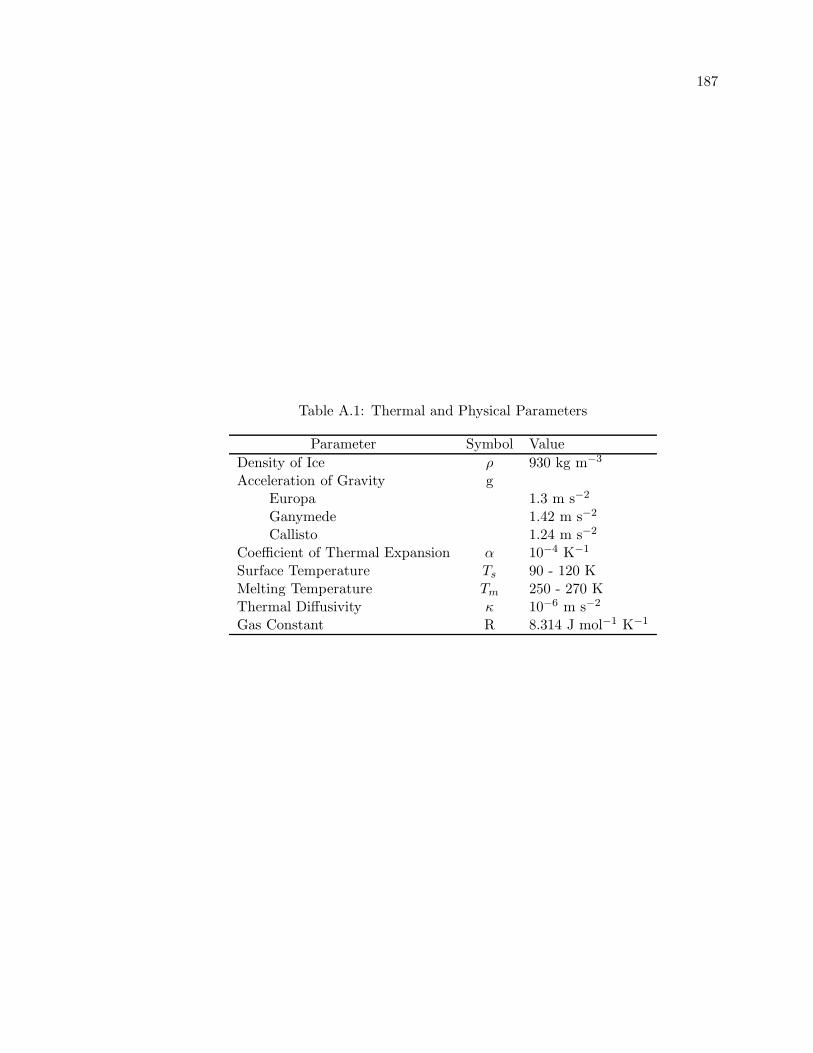
187

Table A.1: Thermal and Physical Parameters

Parameter Symbol Value

Density of Ice ρ 930 kg m−3

Acceleration of Gravity gEuropa 1.3 m s−2

Ganymede 1.42 m s−2

Callisto 1.24 m s−2

Coefficient of Thermal Expansion α 10−4 K−1

Surface Temperature Ts 90 - 120 KMelting Temperature Tm 250 - 270 KThermal Diffusivity κ 10−6 m s−2

Gas Constant R 8.314 J mol−1 K−1

188

Table A.2: Rheological Parameters, after Goldsby and Kohlstedt (2001). † for Tm = 260K.

Rheology A (mp Pa−n s−1) n p Q∗ (kJ mol−1)

Volume Diffusion 3.5 × 10−10 † 1 2 59.4Basal Slip 2.2 × 10−7 2.4 0 60Grain Boundary Sliding 6.2 × 10−14 1.8 1.4 49Dislocation Creep 4.0 × 10−19 4.0 0 60

Appendix B

Selected Input Parameters

190

Table B.1: Selected input parameters for simulations used to determine the criticalRayleigh number and wavelength for convection in ice I with GBS rheology (Chapter2).

Run Name Ra1 δT/∆T k n Ts Tm E

l1016 5.90 × 104 0.05 1.667 1.8 110 260 21.83l1030 5.60 × 104 0.05 1.429 1.8 110 260 21.83l1046 5.60 × 104 0.05 1.25 1.8 110 260 21.83l1065 5.80 × 104 0.05 1.111 1.8 110 260 21.83l1085 6.20 × 104 0.05 1 1.8 110 260 21.83l1144 9.60 × 104 0.05 0.667 1.8 110 260 21.83l1104 8.10 × 104 0.05 0.8 1.8 110 260 21.83l1127 8.80 × 104 0.05 0.727 1.8 110 260 21.83l1162 5.50 × 104 0.05 1.379 1.8 110 260 21.83l1173 5.50 × 104 0.05 1.333 1.8 110 260 21.83l1184 5.50 × 104 0.05 1.365 1.8 110 260 21.83l1202 1.60 × 105 0.005 1.365 1.8 110 260 21.83l1207 1.20 × 105 0.01 1.365 1.8 110 260 21.83l1214 7.70 × 104 0.025 1.365 1.8 110 260 21.83l1220 5.50 × 104 0.05 1.365 1.8 110 260 21.83l1225 4.60 × 104 0.075 1.365 1.8 110 260 21.83l1231 4.00 × 104 0.1 1.365 1.8 110 260 21.83l1301 2.00 × 105 0.005 1.365 1.8 100 260 20.46l1312 1.50 × 105 0.01 1.365 1.8 100 260 20.46l1328 9.30 × 104 0.025 1.365 1.8 100 260 20.46l1339 6.70 × 104 0.05 1.365 1.8 100 260 20.46l1349 5.50 × 104 0.075 1.365 1.8 100 260 20.46l1361 4.70 × 104 0.1 1.365 1.8 100 260 20.46l1403 1.60 × 105 0.005 1.365 1.8 110 270 20.46l1413 1.20 × 105 0.01 1.365 1.8 110 270 20.46l1426 7.60 × 104 0.025 1.365 1.8 110 270 20.46

191

Table B.2: Selected input parameters for simulations used to determine the criticalRayleigh number and wavelength for convection in ice I with GBS rheology (continued).


l1436 5.50 × 104 0.05 1.365 1.8 110 270 20.46l1447 4.50 × 104 0.075 1.365 1.8 110 270 20.46l1458 3.90 × 104 0.1 1.365 1.8 110 270 20.46l1502 2.40 × 105 0.005 1.365 1.8 90 260 19.26l1514 1.80 × 105 0.01 1.365 1.8 90 260 19.26l1522 1.20 × 105 0.025 1.365 1.8 90 260 19.26l1534 7.97 × 104 0.05 1.365 1.8 90 260 19.26l1552 6.50 × 104 0.075 1.365 1.8 90 260 19.26l1561 5.60 × 104 0.1 1.365 1.8 90 260 19.26l1607 1.30 × 105 0.005 1.365 1.8 120 260 23.39l1616 1.00 × 105 0.01 1.365 1.8 120 260 23.39l1630 6.20 × 104 0.025 1.365 1.8 120 260 23.39l1633 4.50 × 104 0.05 1.365 1.8 120 260 23.39l1644 3.70 × 104 0.075 1.365 1.8 120 260 23.39l1656 3.30 × 104 0.1 1.365 1.8 120 260 23.39l1656 3.30 × 104 0.1 1.365 1.8 120 260 23.39l2434 3.10 × 104 0.35 1 1.8 90 260 19.26l2440 2.70 × 104 0.35 1 1.8 100 260 20.46l2442 2.20 × 104 0.35 1 1.8 110 260 21.83l2450 1.90 × 104 0.35 1 1.8 120 260 23.39

192

Table B.3: Selected input parameters for simulations used to determine the criticalRayleigh number and wavelength for convection in ice I with basal slip rheology (Chapter2).


l1703 3.20 × 104 0.05 1.667 2.4 110 260 20.05l1715 3.10 × 104 0.05 1.429 2.4 110 260 20.05l1726 3.10 × 104 0.05 1.25 2.4 110 260 20.05l1735 3.30 × 104 0.05 1.111 2.4 110 260 20.05l1748 3.60 × 104 0.05 1 2.4 110 260 20.05l1759 4.70 × 104 0.05 0.8 2.4 110 260 20.05l1770 5.80 × 104 0.05 0.667 2.4 110 260 20.05l1781 3.10 × 104 0.05 1.333 2.4 110 260 20.05l1789 3.10 × 104 0.05 1.379 2.4 110 260 20.05l1795 3.10 × 104 0.05 1.29 2.4 110 260 20.05l1801 1.20 × 105 0.005 1.333 2.4 110 260 20.05l1808 8.00 × 104 0.01 1.333 2.4 110 260 20.05l1814 4.60 × 104 0.025 1.333 2.4 110 260 20.05l1819 2.40 × 104 0.075 1.333 2.4 110 260 20.05l1826 2.00 × 104 0.1 1.333 2.4 110 260 20.05l1842 1.80 × 105 0.005 1.333 2.4 90 260 17.69l1847 1.20 × 105 0.01 1.333 2.4 90 260 17.69l1855 6.60 × 104 0.025 1.333 2.4 90 260 17.69l1858 4.30 × 104 0.05 1.333 2.4 90 260 17.69l1865 3.30 × 104 0.075 1.333 2.4 90 260 17.69l1872 2.80 × 104 0.1 1.333 2.4 90 260 17.69l1903 1.50 × 105 0.005 1.333 2.4 100 260 18.79l1913 1.00 × 105 0.01 1.333 2.4 100 260 18.79

193

Table B.4: Selected input parameters for simulations used to determine the criticalRayleigh number and wavelength for convection in ice I with basal slip rheology (con-tinued).


l1925 5.60 × 104 0.025 1.333 2.4 100 260 18.79l1939 3.70 × 104 0.05 1.333 2.4 100 260 18.79l1950 2.80 × 104 0.075 1.333 2.4 100 260 18.79l1961 2.40 × 104 0.1 1.333 2.4 100 260 18.79l2002 1.00 × 105 0.005 1.333 2.4 120 260 21.48l2015 6.60 × 104 0.01 1.333 2.4 120 260 21.48l2030 3.80 × 104 0.025 1.333 2.4 120 260 21.48l2038 2.60 × 104 0.05 1.333 2.4 120 260 21.48l2048 2.00 × 104 0.075 1.333 2.4 120 260 21.48l2058 1.70 × 104 0.1 1.333 2.4 120 260 21.48l2101 1.20 × 105 0.005 1.333 2.4 110 250 21.48l2108 8.00 × 104 0.01 1.333 2.4 110 250 21.48l2113 4.70 × 104 0.025 1.333 2.4 110 250 21.48l2122 3.10 × 104 0.05 1.333 2.4 110 250 21.48l2125 2.40 × 104 0.075 1.333 2.4 110 250 21.48l2134 2.00 × 104 0.1 1.333 2.4 110 250 21.48l2403 9.80 × 103 0.35 1 2.4 110 260 20.05l2407 1.40 × 104 0.35 1 2.4 90 260 17.69l2414 1.20 × 104 0.35 1 2.4 100 260 18.79l2418 8.30 × 103 0.35 1 2.4 120 260 21.48

194

Table B.5: Selected input parameters for simulations used to determine the criticalRayleigh number and wavelength for convection in ice I with composite rheology (Chap-ter 3).

Run Name Rao δT/∆T k d (m)

gk2053 7.32 × 103 0.02 1.143 2 × 10−2

gk2057 7.16 × 103 0.025 1.143 2 × 10−2

gk2063 6.82 × 103 0.035 1.143 2 × 10−2

gk2027 6.30 × 103 0.05 1.143 2 × 10−2

gk2072 5.57 × 103 0.075 1.143 2 × 10−2

gk2078 5.01 × 103 0.1 1.143 2 × 10−2

gk1943 3.17 × 102 0.02 1.143 3 × 10−2

gk1951 3.11 × 102 0.025 1.143 3 × 10−2

gk1954 2.97 × 102 0.035 1.143 3 × 10−2

gk1931 2.74 × 102 0.05 1.143 3 × 10−2

gk1960 2.42 × 102 0.075 1.143 3 × 10−2

gk1966 2.17 × 102 0.1 1.143 3 × 10−2

gk1824 2.08 × 10−2 0.025 1.143 10−1

gk1836 1.82 × 10−2 0.05 1.143 10−1

gk1853 1.61 × 10−2 0.075 1.143 10−1

gk1874 2.11 × 10−2 0.02 1.143 10−1

gk1869 1.97 × 10−2 0.035 1.143 10−1

gk1722 2.45 × 105 0.025 1.143 10−2

gk1190 2.13 × 105 0.05 1.143 10−2

gk1738 1.91 × 105 0.075 1.143 10−2

gk1741 1.74 × 105 0.1 1.143 10−2

gk1752 2.57 × 105 0.02 1.143 10−2

gk1763 2.29 × 105 0.035 1.143 10−2

gk1773 1.46 × 105 0.2 1.143 10−2

gk1202 2.53 × 106 0.025 1.143 10−3

gk1365 2.19 × 106 0.05 1.143 10−3

gk1208 1.93 × 106 0.075 1.143 10−3

gk1212 1.75 × 106 0.1 1.143 10−3

gk1227 2.77 × 106 0.02 1.143 10−4

gk1219 2.49 × 106 0.035 1.143 10−4

gk1232 1.50 × 106 0.2 1.143 10−4

gk1616 2.66 × 106 0.025 1.143 10−4

gk1620 2.30 × 106 0.05 1.143 10−4

gk1626 2.03 × 106 0.075 1.143 10−4

gk1633 1.82 × 106 0.1 1.143 10−4

gk1639 2.77 × 106 0.02 1.143 10−4

gk1644 2.49 × 106 0.035 1.143 10−4

gk1652 1.48 × 106 0.2 1.143 10−4

195

Table B.6: Selected input parameters for simulations used to determine the criticalRayleigh number and wavelength for convection in ice I with composite rheology (Chap-ter 3), continued.

Run Name Rao δT/∆T k d (m)

gk1013 1.85 × 10−2 0.05 1.333 10−1

gk1040 1.83 × 10−2 0.05 1.25 10−1

gk1052 1.82 × 10−2 0.05 1.176 10−1

gk1062 1.82 × 10−2 0.05 1.111 10−1

gk1067 1.89 × 10−2 0.05 0.909 10−1

gk1083 1.83 × 10−2 0.05 1.052 10−1

gk1087 1.85 × 10−2 0.05 1 10−1

gk1100 2.20 × 105 0.05 1.428 10−2

gk1114 2.17 × 105 0.05 1.333 10−2

gk1128 2.14 × 105 0.05 1.25 10−2

gk1140 2.13 × 105 0.05 1.176 10−2

gk1190 2.13 × 105 0.05 1.143 10−2

gk1151 2.13 × 105 0.05 1.111 10−2

gk1198 2.15 × 105 0.05 1 10−2

gk1156 2.19 × 105 0.05 0.909 10−2

gk1300 2.25 × 106 0.05 1.428 10−3

gk1309 2.22 × 106 0.05 1.333 10−3

gk1312 2.20 × 106 0.05 1.25 10−3

gk1319 2.19 × 106 0.05 1.176 10−3

gk1365 2.19 × 106 0.05 1.143 10−3

gk1325 2.19 × 106 0.05 1.111 10−3

gk1377 2.20 × 106 0.05 1.052 10−3

gk1372 2.21 × 106 0.05 1 10−3

gk1503 2.37 × 106 0.05 1.428 10−4

gk1508 2.33 × 106 0.05 1.333 10−4

gk1516 2.31 × 106 0.05 1.25 10−4

gk1518 2.30 × 106 0.05 1.176 10−4

gk1524 2.30 × 106 0.05 1.111 10−4

gk1534 2.31 × 106 0.05 1.052 10−4

gk1539 2.32 × 106 0.05 1 10−4

gk1545 2.37 × 106 0.05 0.909 10−4

196

Table B.7: Weighting values for the composite rheology for ice I used in Chapters 3, 4,and 5.

d (m) βdisl βGBS βbs

1 × 10−1 1.48 × 1020 2.01 × 10−13 2.09 × 10−22

3 × 10−2 9.71 × 1015 2.84 × 10−12 6.77 × 10−20

2 × 10−2 3.79 × 1014 6.94 × 10−12 4.74 × 10−19

1 × 10−2 1.48 × 1012 3.19 × 10−11 1.32 × 10−17

3 × 10−3 9.71 × 107 4.50 × 10−10 4.27 × 10−15

1 × 10−3 1.48 × 104 5.05 × 10−9 8.33 × 10−13

3 × 10−4 9.71 × 10−1 7.14 × 10−8 2.69 × 10−10

1 × 10−4 1.48 × 10−4 8.00 × 10−7 5.26 × 10−8

197

Table B.8: Input parameters from simulations used to determine the convective heatflux and mass flux in Chapters 4 and 5.

Run Name Shell Thickness (km) d (m) δT/∆T Rao Time Step

a996 20 10−4 0.05 5.882 × 106 60000a963 20 3 × 10−4 0.05 6.536 × 105 N/Aa962 20 3 × 10−4 0.25 6.536 × 105 N/Aa995 20 10−3 0.05 3.102 × 106 25000a994 20 10−3 0.25 9.191 × 105 N/Aa974 20 3 × 10−3 0.05 6.536 × 103 N/Aa973 20 3 × 10−3 0.25 6.536 × 103 N/Aa989 20 10−2 0.05 5.882 × 102 N/Aa988 20 10−2 0.25 5.882 × 102 N/Aa981 20 3 × 10−2 0.05 6.536 × 101 N/Aa980 20 3 × 10−2 0.25 6.536 × 101 N/Aa970 35 10−4 0.05 3.153 × 107 55000a971 35 3 × 10−4 0.25 3.503 × 106 25000a969 35 3 × 10−2 0.05 3.503 × 102 25000a997 50 10−4 0.05 9.191 × 107 75000a967 50 3 × 10−4 0.05 1.021 × 107 50000a993 50 10−3 0.05 9.191 × 105 N/Aa992 50 10−3 0.25 5.882 × 104 N/Aa987 50 10−2 0.05 9.191 × 103 N/Aa986 50 10−2 0.25 9.191 × 103 N/Aa979 50 3 × 10−2 0.05 1.021 × 103 40000

198

Table B.9: Input parameters from simulations used to determine the convective heatflux and mass flux in Chapters 4 and 5 (continued).

Run Name Shell Thickness (km) d (m) δT/∆T Rao Time Step

a956 60 10−4 0.05 1.588 × 108 75000a955 60 3 × 10−4 0.05 1.765 × 107 45000a961 60 10−3 0.05 1.588 × 106 N/Aa959 60 10−3 0.25 1.588 × 106 15000a960 60 3 × 10−2 0.05 1.765 × 103 75000a998 75 10−4 0.05 3.102 × 108 75000a968 75 3 × 10−4 0.05 3.447 × 107 55000a991 75 10−3 0.05 5.882 × 104 N/Aa985 75 10−2 0.05 3.102 × 104 N/Aa984 75 10−2 0.25 3.102 × 104 N/Aa977 75 3 × 10−2 0.05 3.447 × 103 50000a965 85 10−4 0.05 4.516 × 108 N/Aa958 85 3 × 10−4 0.05 5.017 × 107 75000a957 85 10−3 0.05 4.516 × 106 N/Aa964 85 3 × 10−2 0.05 5.017 × 103 70000a999 100 10−4 0.05 7.353 × 108 N/Aa978 100 3 × 10−4 0.05 8.170 × 103 N/Aa976 100 3 × 10−4 0.05 8.170 × 107 75000a990 100 10−3 0.05 7.353 × 106 30000a975 100 3 × 10−3 0.05 8.170 × 105 N/Aa972 100 3 × 10−3 0.25 8.170 × 105 N/Aa983 100 10−2 0.05 7.353 × 104 N/Aa982 100 10−2 0.25 7.353 × 104 N/Aa966 150 3 × 10−3 0.05 2.757 × 106 N/A

convection in ice i with non-newtonian rheology ... · convection in ice i with non-newtonian...

Documents