controlling for scanner-to- scanner variance in multicenter fmri studies: covariation with...
TRANSCRIPT
Controlling for Scanner-to-Scanner Variance in Multicenter FMRI Studies: Covariation with
Signal-to-Fluctuation Noise Ratio (SFNR)
Lee Friedman, Ph.D.
And
Gary Glover, Ph.D.
Overall Goal
• To evaluate scanner effects on brain activation patterns in multisite fMRI studies
• To determine the cause of these scanner effects
• To develop methods to reduce such scanner effects
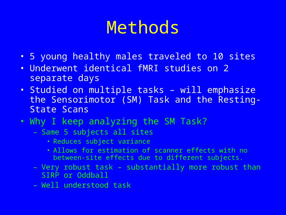
Methods
• 5 young healthy males traveled to 10 sites• Underwent identical fMRI studies on 2 separate days• Studied on multiple tasks – will emphasize the
Sensorimotor (SM) Task and the Resting-State Scans• Why I keep analyzing the SM Task?
– Same 5 subjects all sites• Reduces subject variance• Allows for estimation of scanner effects with no between-site effects
due to different subjects.
– Very robust task – substantially more robust than SIRP or Oddball
– Well understood task


Functional Image Acquisition
• Pulse sequence = EPI or Spiral GRE• Scan plane = oblique axial, AC-PC, copy T2 • FOV = 220 mm• 35 slices, contiguous 4mm• TR = 3000ms TE = 30ms (3T/4T), 40ms (1.5T)• FA = 90 degrees• BW >= ±100 kHz• 64x64 matrix, 1 shot
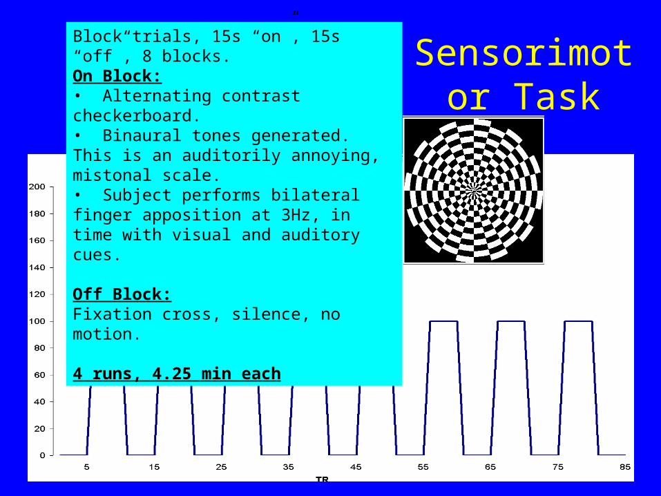
Sensorimotor Task
Block trials, 15s “on”, 15s “off”, 8 blocks.On Block:• Alternating contrast checkerboard.• Binaural tones generated. This is an auditorily annoying, mistonal scale.• Subject performs bilateral finger apposition at 3Hz, in time with visual and auditory cues.
Off Block: Fixation cross, silence, no motion.
4 runs, 4.25 min each
Resting-State Scans
• Stare at fixation cross.
• Two runs, 85 TRs (4.25 min)

We Measured 6 Types of SFNRbut Will Focus on 2 for Simplicity
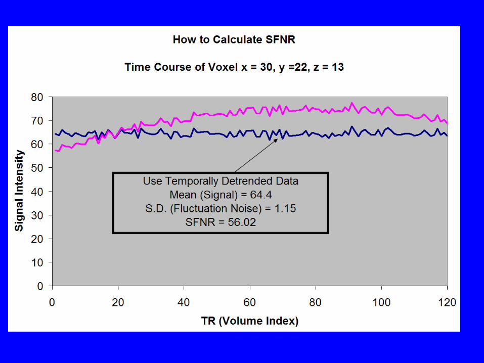
• SFNR – GM – REST– Based on Resting-State Data– (Mean GM intensity)/(SD Gray Matter Intensity)
• SFNR – GM – RESID– Based on the SM Task, not Resting-State– GLM model intercept is used as Signal– SD of GLM Model Residuals used as
Fluctuation Noise.
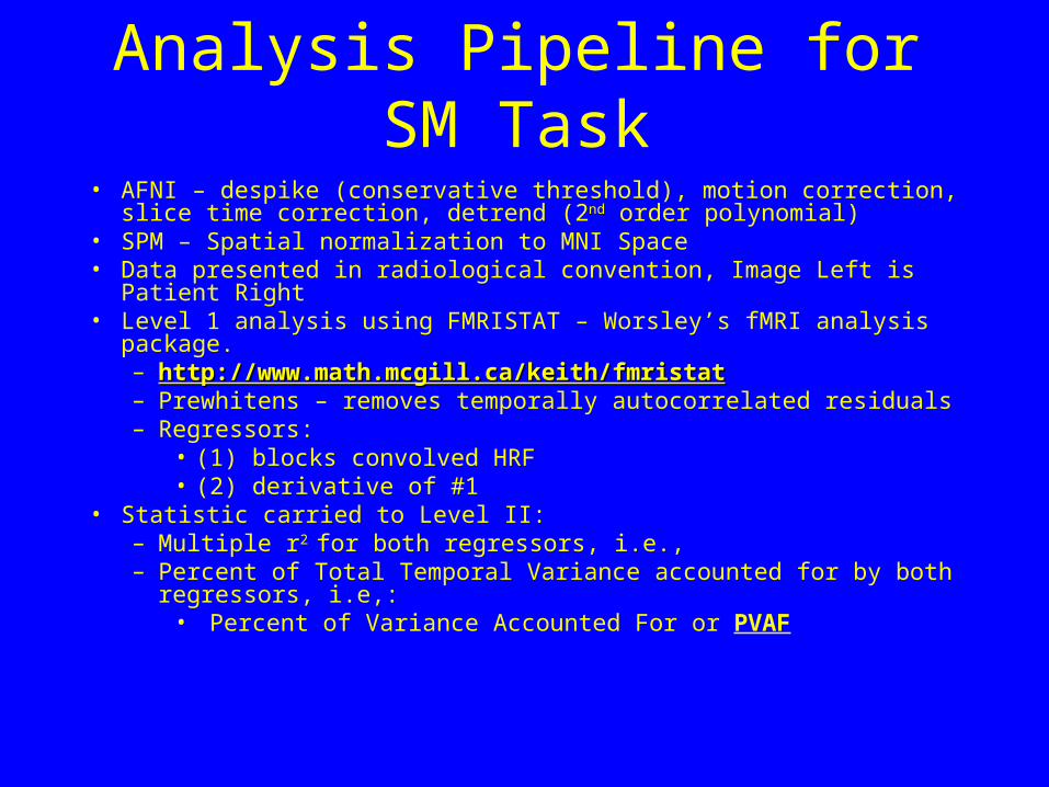
Analysis Pipeline for SM Task
• AFNI – despike (conservative threshold), motion correction, slice time correction, detrend (2nd order polynomial)
• SPM – Spatial normalization to MNI Space• Data presented in radiological convention, Image Left is Patient Right• Level 1 analysis using FMRISTAT – Worsley’s fMRI analysis package.
– http://www.math.mcgill.ca/keith/fmristathttp://www.math.mcgill.ca/keith/fmristat– Prewhitens – removes temporally autocorrelated residuals – Regressors:
• (1) blocks convolved HRF• (2) derivative of #1
• Statistic carried to Level II:– Multiple r2 for both regressors, i.e.,– Percent of Total Temporal Variance accounted for by both
regressors, i.e,:• Percent of Variance Accounted For or PVAF
Why Choose PVAF as Level I Statistic ? • FMRI researchers are primarily interested in evaluating
brain activation patterns.• Brain activation patterns are typically produced by
thresholding statistical maps (t-maps, F-maps, etc …) and looking only at voxels activated above a statistical threshold.
• Efforts to homogenize brain activation effect size (like PVAF) will result in homogenization of patterns of activation across sites.
• Since beta-weights alone carry no information about the statistical significance or CNR of an effect, they alone are poor candidates for use in homogenizing activations patterns across sites. They are useful in homogenizing signal amplitude across sites, which is important.
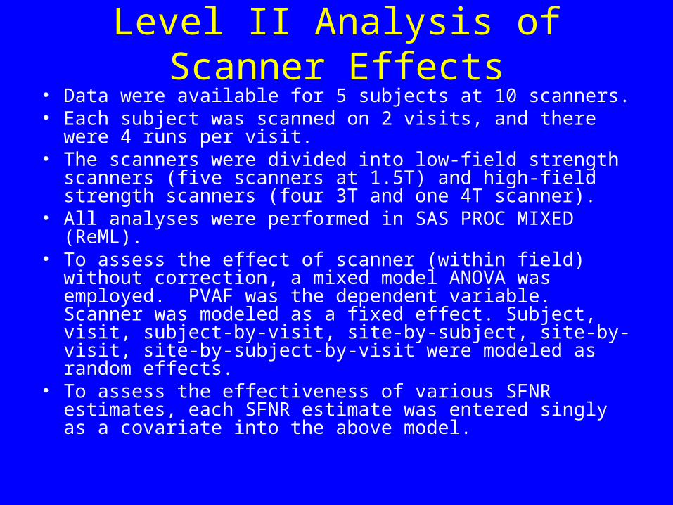
Level II Analysis of Scanner Effects• Data were available for 5 subjects at 10 scanners.• Each subject was scanned on 2 visits, and there were 4 runs
per visit. • The scanners were divided into low-field strength scanners
(five scanners at 1.5T) and high-field strength scanners (four 3T and one 4T scanner).
• All analyses were performed in SAS PROC MIXED (ReML).• To assess the effect of scanner (within field) without
correction, a mixed model ANOVA was employed. PVAF was the dependent variable. Scanner was modeled as a fixed effect. Subject, visit, subject-by-visit, site-by-subject, site-by-visit, site-by-subject-by-visit were modeled as random effects.
• To assess the effectiveness of various SFNR estimates, each SFNR estimate was entered singly as a covariate into the above model.
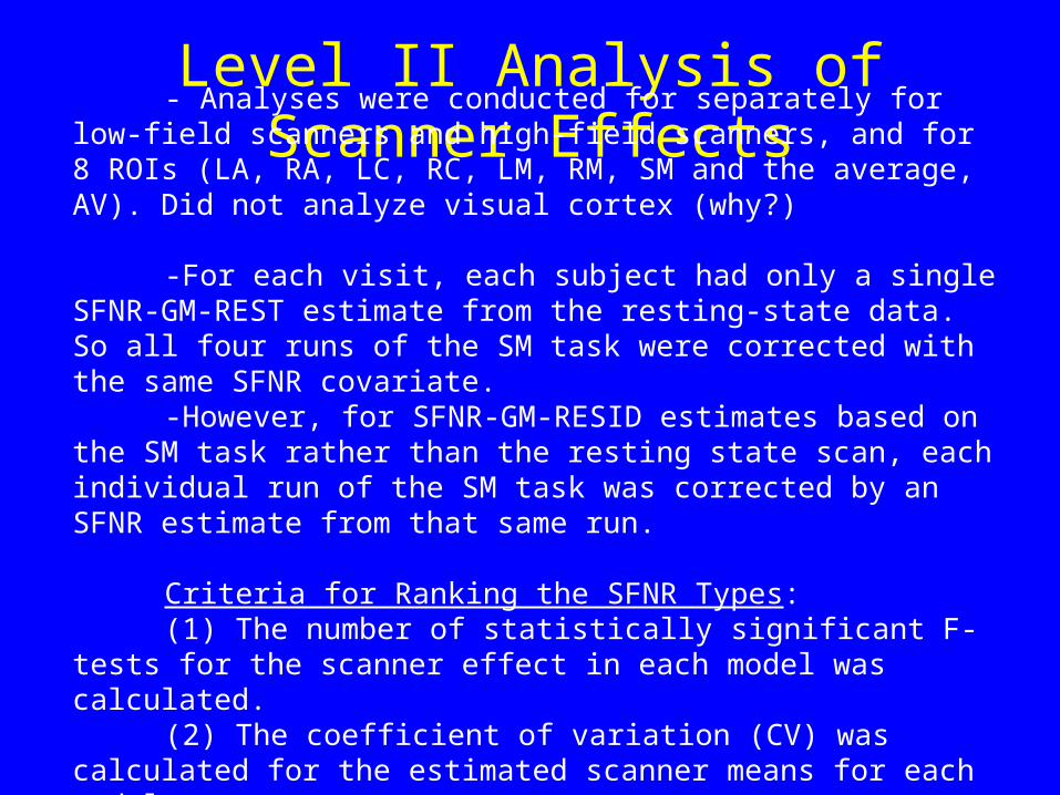
Level II Analysis of Scanner Effects- Analyses were conducted for separately for low-field scanners
and high-field scanners, and for 8 ROIs (LA, RA, LC, RC, LM, RM, SM and the average, AV). Did not analyze visual cortex (why?)
-For each visit, each subject had only a single SFNR-GM-REST estimate from the resting-state data. So all four runs of the SM task were corrected with the same SFNR covariate.
-However, for SFNR-GM-RESID estimates based on the SM task rather than the resting state scan, each individual run of the SM task was corrected by an SFNR estimate from that same run.
Criteria for Ranking the SFNR Types: (1) The number of statistically significant F-tests for the scanner
effect in each model was calculated. (2) The coefficient of variation (CV) was calculated for the
estimated scanner means for each model.
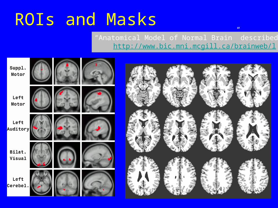
ROIs and Masks“Anatomical Model of Normal Brain” described at:
http://www.bic.mni.mcgill.ca/brainweb/l
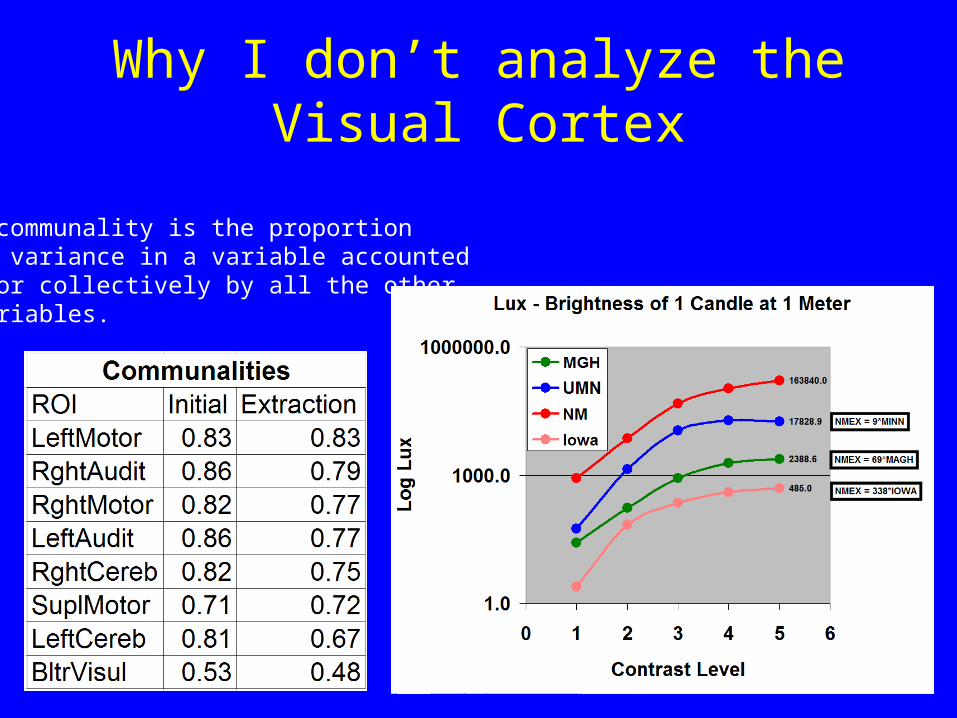
Why I don’t analyze the Visual Cortex
A communality is the proportionof variance in a variable accounted for collectively by all the other variables.
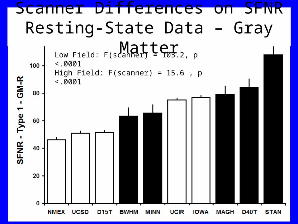
Scanner Differences on SFNRResting-State Data – Gray Matter
Low Field: F(scanner) = 103.2, p <.0001High Field: F(scanner) = 15.6 , p <.0001
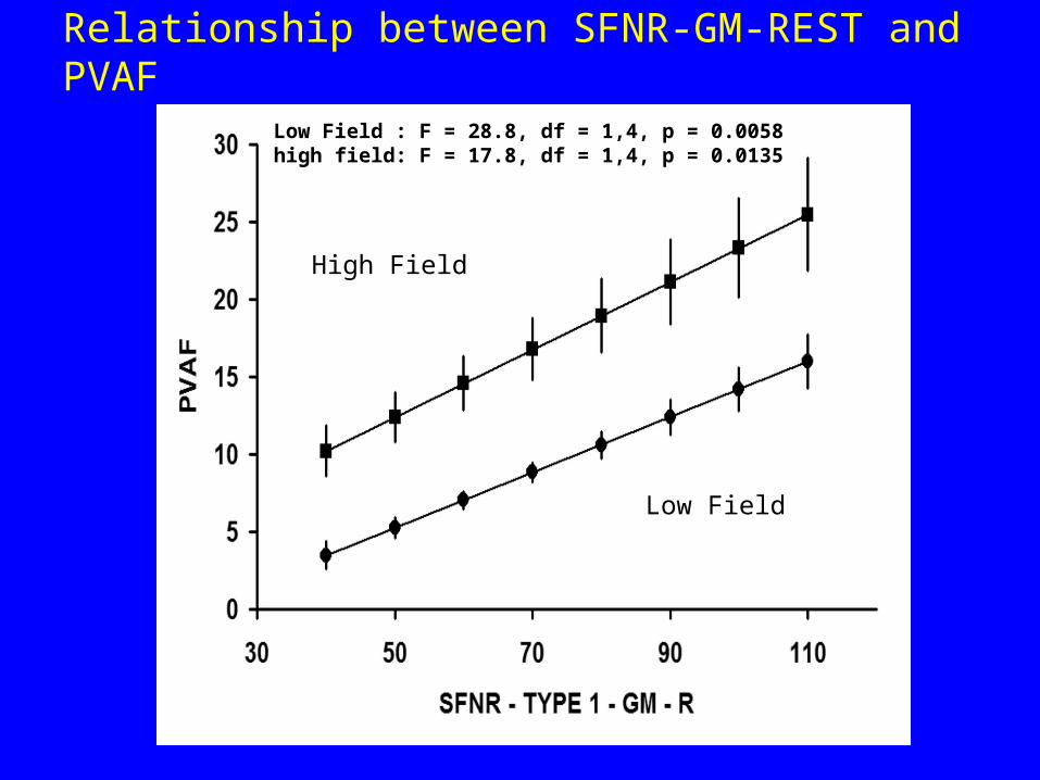
Relationship between SFNR-GM-REST and PVAF
Low Field : F = 28.8, df = 1,4, p = 0.0058 high field: F = 17.8, df = 1,4, p = 0.0135
Low Field
High Field
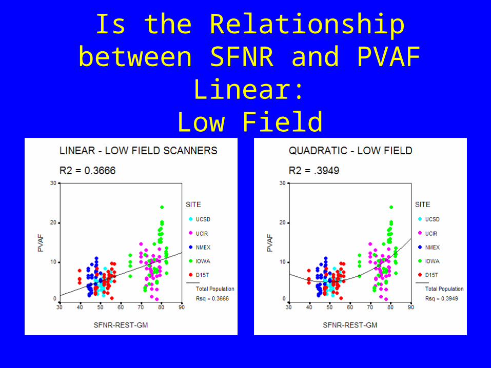
Is the Relationship between SFNR and PVAF Linear:
Low Field

Is the Relationship between SFNR and PVAF Linear?
High Field
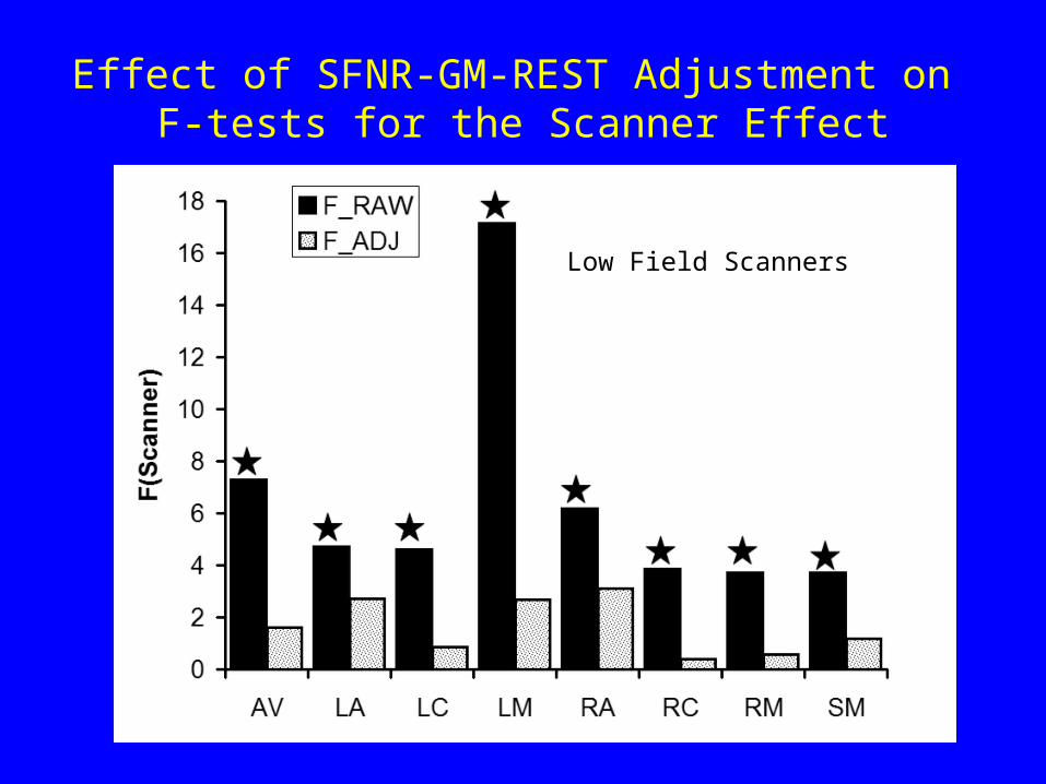
Effect of SFNR-GM-REST Adjustment on F-tests for the Scanner Effect
Low Field Scanners
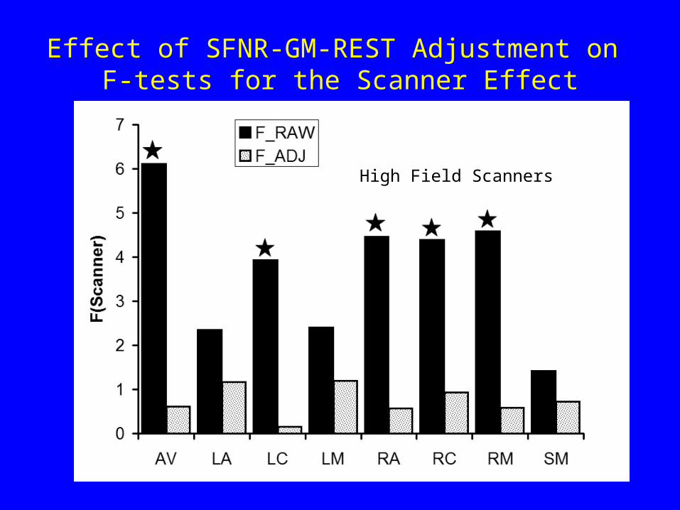
Effect of SFNR-GM-REST Adjustment on F-tests for the Scanner Effect
High Field Scanners
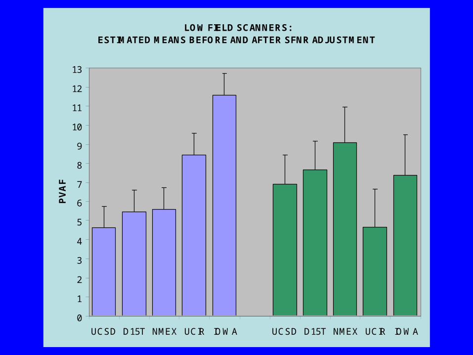
LOW FIELD SCANNERS: ESTIMATED MEANS BEFORE AND AFTER SFNR ADJUSTMENT
0
1
2
3
4
5
6
7
8
9
10
11
12
13
UCSD D15T NMEX UCIR IOWA UCSD D15T NMEX UCIR IOWA
PV
AF
NO ADJUSTMENTCV = 0.40
ADJUSTMENT WITH SFNR-GM-RESTCV = 0.22
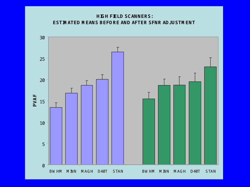
HIGH FIELD SCANNERS: ESTIMATED MEANS BEFORE AND AFTER SFNR ADJUSTMENT
0
5
10
15
20
25
30
BWHM MINN MAGH D40T STAN BWHM MINN MAGH D40T STAN
PV
AF
NO ADJUSTMENTCV = 0.25
ADJUSTMENT WITH SFNR-GM-RESTCV = 0.14
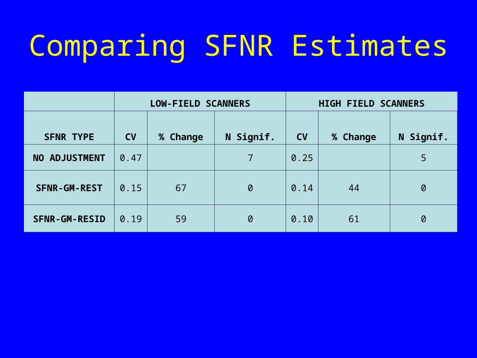
Comparing SFNR Estimates
LOW-FIELD SCANNERS HIGH FIELD SCANNERS
SFNR TYPE CV % Change N Signif. CV % Change N Signif.
NO ADJUSTMENT 0.47 7 0.25 5
SFNR-GM-REST 0.15 67 0 0.14 44 0
SFNR-GM-RESID 0.19 59 0 0.10 61 0
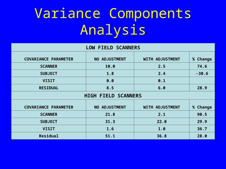
Variance Components Analysis
LOW FIELD SCANNERS
COVARIANCE PARAMETER NO ADJUSTMENT WITH ADJUSTMENT % Change
SCANNER 10.0 2.5 74.6
SUBJECT 1.8 2.4 -30.6
VISIT 0.0 0.1
RESIDUAL 8.5 6.0 28.9
HIGH FIELD SCANNERS
COVARIANCE PARAMETER NO ADJUSTMENT WITH ADJUSTMENT % Change
SCANNER 21.8 2.1 90.5
SUBJECT 31.3 22.0 29.9
VISIT 1.6 1.0 36.7
Residual 51.1 36.8 28.0
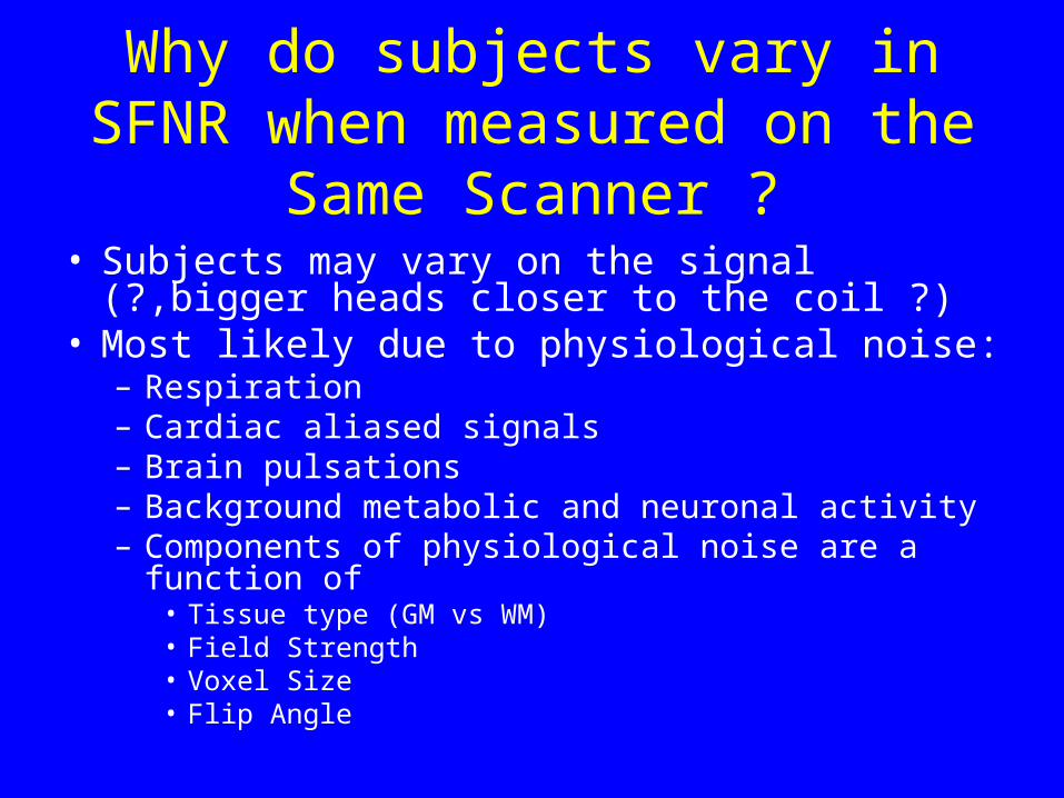
Why do subjects vary in SFNR when measured on the Same
Scanner ?• Subjects may vary on the signal (?,bigger heads
closer to the coil ?)• Most likely due to physiological noise:
– Respiration– Cardiac aliased signals– Brain pulsations– Background metabolic and neuronal activity– Components of physiological noise are a function of
• Tissue type (GM vs WM)• Field Strength• Voxel Size• Flip Angle
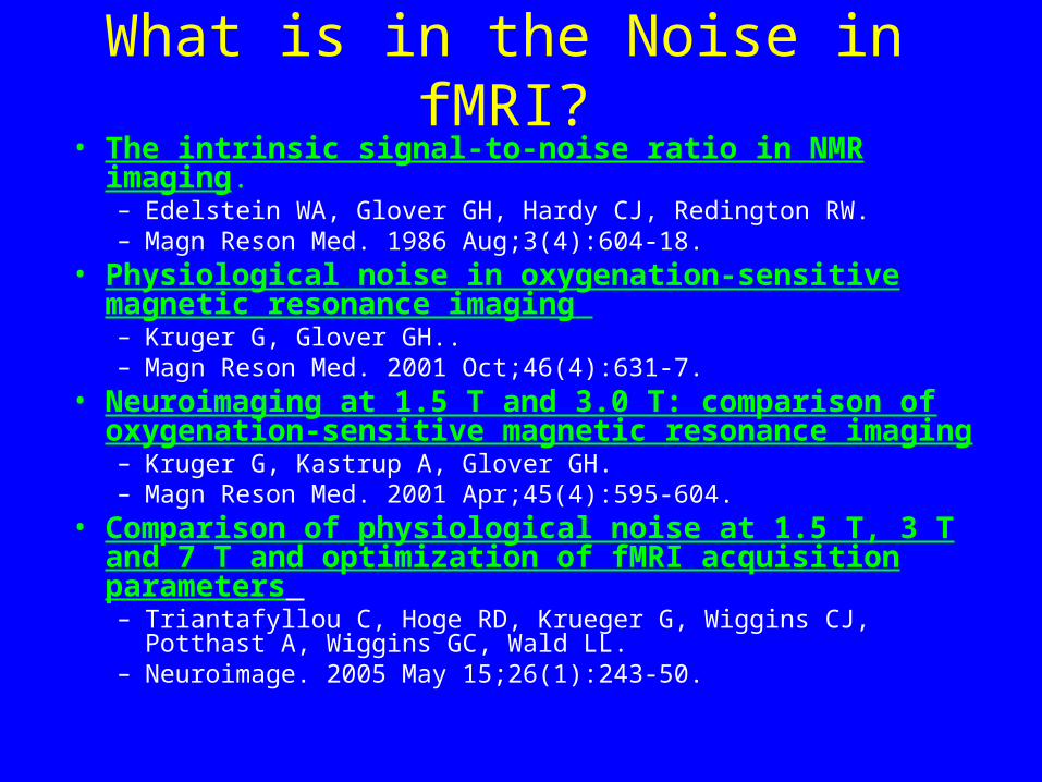
What is in the Noise in fMRI?• The intrinsic signal-to-noise ratio in NMR imaging.
– Edelstein WA, Glover GH, Hardy CJ, Redington RW.– Magn Reson Med. 1986 Aug;3(4):604-18.
• Physiological noise in oxygenation-sensitive magnetic resonance imaging – Kruger G, Glover GH.. – Magn Reson Med. 2001 Oct;46(4):631-7.
• Neuroimaging at 1.5 T and 3.0 T: comparison of oxygenation-sensitive magnetic resonance imaging – Kruger G, Kastrup A, Glover GH. – Magn Reson Med. 2001 Apr;45(4):595-604.
• Comparison of physiological noise at 1.5 T, 3 T and 7 T and optimization of fMRI acquisition parameters – Triantafyllou C, Hoge RD, Krueger G, Wiggins CJ, Potthast A,
Wiggins GC, Wald LL.– Neuroimage. 2005 May 15;26(1):243-50.

Conclusions
• Using SFNR as a covariate is effective in reducing the effect of scanner on activation effect size
• Using an SFNR estimate based on the SM task itself is an effective approach – no resting state data is needed.
• Subject variance due to physiological noise is also controlled with this method.
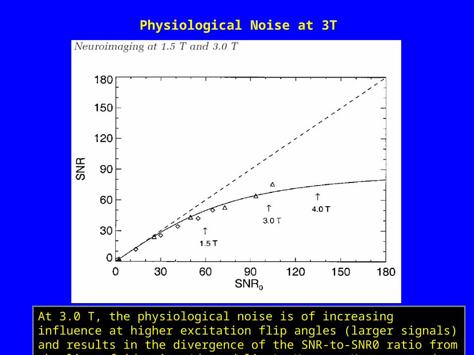
At 3.0 T, the physiological noise is of increasing influence at higher excitation flip angles (larger signals) and results in the divergence of the SNR-to-SNR0 ratio from the line-of identity (dotted line). Kruger, Kastrup, and Glover, 2001
Physiological Noise at 3T
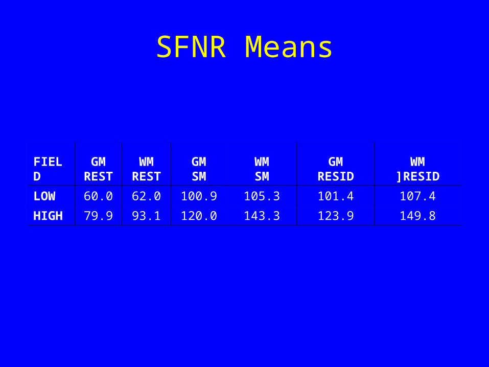
SFNR Means
FIELD
GMREST
WMREST
GMSM
WMSM
GMRESID
WM]RESID
LOW 60.0 62.0 100.9 105.3 101.4 107.4
HIGH 79.9 93.1 120.0 143.3 123.9 149.8