controller synthesis and vibration suppression...

Controller Synthesis and Vibration Suppression Techniques for IndustrialRobotic Manipulators with Joint Flexibilities

by

Michael L Chan

A dissertation submitted in partial satisfaction of the

requirements for the degree of

Doctor of Philosophy

in

Engineering - Mechanical Engineering

in the

Graduate Division

of the

University of California, Berkeley

Committee in charge:

Professor Masayoshi Tomizuka, ChairProfessor J. Karl Hedrick

Professor Ming Gu

Fall 2013

Controller Synthesis and Vibration Suppression Techniques for Industrial

Robotic Manipulators with Joint Flexibilities

Copyright 2013

by

Michael L Chan

1

Abstract

Controller Synthesis and Vibration Suppression Techniques for Industrial RoboticManipulators with Joint Flexibilities

by

Michael L Chan

Doctor of Philosophy in Engineering - Mechanical Engineering

University of California, Berkeley

Professor Masayoshi Tomizuka, Chair

This dissertation focuses on the design of feedback and feedforward controllers for directapplication to industrial manipulators. In this dissertation, an iterative online controllertuning algorithm based on nonlinear programming concepts and extremum seeking controlis introduced and applied to a 6 degree of freedom FANUC M16iB industrial robot. Detailsregarding stepsize selection and gradient estimation for the proposed controller tuning isalso discussed. Experimental results show that the proposed controller tuning method isable to improve robot performance by successively reducing a cost function. Additionally, acontroller tuning framework based off the disturbance observer is also introduced for stablecontroller tuning. The framework is shown to be robustly stable under most practical tuningapplications. The assumptions and constraints of the proposed framework is also detailed.The framework is experimentally verified by sweeping through a variety of controller gainsthat satisfy the framework conditions. Finally, an input shaping technique for applicationto industrial robots with elastic joints is also proposed in this dissertation. The approach issimple to apply and can be easily integrated to existing trajectory generation techniques forindustrial robots. Experimental results show substantial joint vibration suppression duringtransient motions.

i

To my parents

ii

Contents

Contents ii

List of Figures iii

List of Tables v

1 Introduction 11.1 Background . . . . . . . . . . . . . . . . . . . . . . . . . . . . . . . . . . . . 11.2 Motivation and Contribution . . . . . . . . . . . . . . . . . . . . . . . . . . . 11.3 Dissertation Outline . . . . . . . . . . . . . . . . . . . . . . . . . . . . . . . 3

2 System Modeling, Hardware Description, and System Identification 52.1 Introduction . . . . . . . . . . . . . . . . . . . . . . . . . . . . . . . . . . . . 52.2 Two Mass Model . . . . . . . . . . . . . . . . . . . . . . . . . . . . . . . . . 52.3 Multiple Degree of Freedom Robot Model . . . . . . . . . . . . . . . . . . . 92.4 Hardware and Software Setup . . . . . . . . . . . . . . . . . . . . . . . . . . 102.5 System Identification . . . . . . . . . . . . . . . . . . . . . . . . . . . . . . . 142.6 Chapter Summary . . . . . . . . . . . . . . . . . . . . . . . . . . . . . . . . 18

3 Sensor-based Feedback Controller Tuning of Robot Manipulators byNonlinear Programming 263.1 Introduction . . . . . . . . . . . . . . . . . . . . . . . . . . . . . . . . . . . . 263.2 Nonlinear Programming . . . . . . . . . . . . . . . . . . . . . . . . . . . . . 263.3 Controller Tuning Process . . . . . . . . . . . . . . . . . . . . . . . . . . . . 303.4 Barrier Functions . . . . . . . . . . . . . . . . . . . . . . . . . . . . . . . . . 313.5 Stepsize Selection . . . . . . . . . . . . . . . . . . . . . . . . . . . . . . . . . 353.6 Initial Condition Selection . . . . . . . . . . . . . . . . . . . . . . . . . . . . 363.7 Experimental Results . . . . . . . . . . . . . . . . . . . . . . . . . . . . . . . 423.8 Chapter Summary . . . . . . . . . . . . . . . . . . . . . . . . . . . . . . . . 44

4 A Disturbance Observer Framework for Stable Feedback Controller Tuning 514.1 Introduction . . . . . . . . . . . . . . . . . . . . . . . . . . . . . . . . . . . . 51

iii

4.2 Traditional Disturbance Observer . . . . . . . . . . . . . . . . . . . . . . . . 514.3 Disturbance Observer Tuning Framework . . . . . . . . . . . . . . . . . . . . 524.4 Results . . . . . . . . . . . . . . . . . . . . . . . . . . . . . . . . . . . . . . . 594.5 Chapter Summary . . . . . . . . . . . . . . . . . . . . . . . . . . . . . . . . 60

5 An Input Shaping Method to Suppress Transient Vibrations In FlexibleJoint Robotic Manipulators 625.1 Introduction . . . . . . . . . . . . . . . . . . . . . . . . . . . . . . . . . . . . 625.2 Input Shaping . . . . . . . . . . . . . . . . . . . . . . . . . . . . . . . . . . . 625.3 Theory . . . . . . . . . . . . . . . . . . . . . . . . . . . . . . . . . . . . . . . 635.4 Results . . . . . . . . . . . . . . . . . . . . . . . . . . . . . . . . . . . . . . . 675.5 Chapter Summary . . . . . . . . . . . . . . . . . . . . . . . . . . . . . . . . 74

6 Conclusions 806.1 Chapter Summary . . . . . . . . . . . . . . . . . . . . . . . . . . . . . . . . 806.2 Future Work . . . . . . . . . . . . . . . . . . . . . . . . . . . . . . . . . . . . 81

Bibliography 82

List of Figures

2.1 Two inertial model of an indirect drive mechanism . . . . . . . . . . . . . . . . 72.2 Harmonic drive components . . . . . . . . . . . . . . . . . . . . . . . . . . . . . 82.3 FANUC M16iB industrial manipulator . . . . . . . . . . . . . . . . . . . . . . . 112.4 Joint naming and rotating conventions for the FANUC M16iB robot . . . . . . 122.5 FANUC M16iB robot system setup scheme . . . . . . . . . . . . . . . . . . . . . 132.6 Decentralized feedback controller scheme . . . . . . . . . . . . . . . . . . . . . . 152.7 Controller for system identification . . . . . . . . . . . . . . . . . . . . . . . . . 162.8 Robot postures for system identification . . . . . . . . . . . . . . . . . . . . . . 192.9 System identification result for joint 1: uref ⇒ θm (o: sine sweep results, x: sine

by sine results) . . . . . . . . . . . . . . . . . . . . . . . . . . . . . . . . . . . . 202.10 System identification result for joint 2: uref ⇒ θm (o: sine sweep results, x: sine

by sine results) . . . . . . . . . . . . . . . . . . . . . . . . . . . . . . . . . . . . 212.11 System identification result for joint 3: uref ⇒ θm (o: sine sweep results, x: sine

by sine results) . . . . . . . . . . . . . . . . . . . . . . . . . . . . . . . . . . . . 22

iv

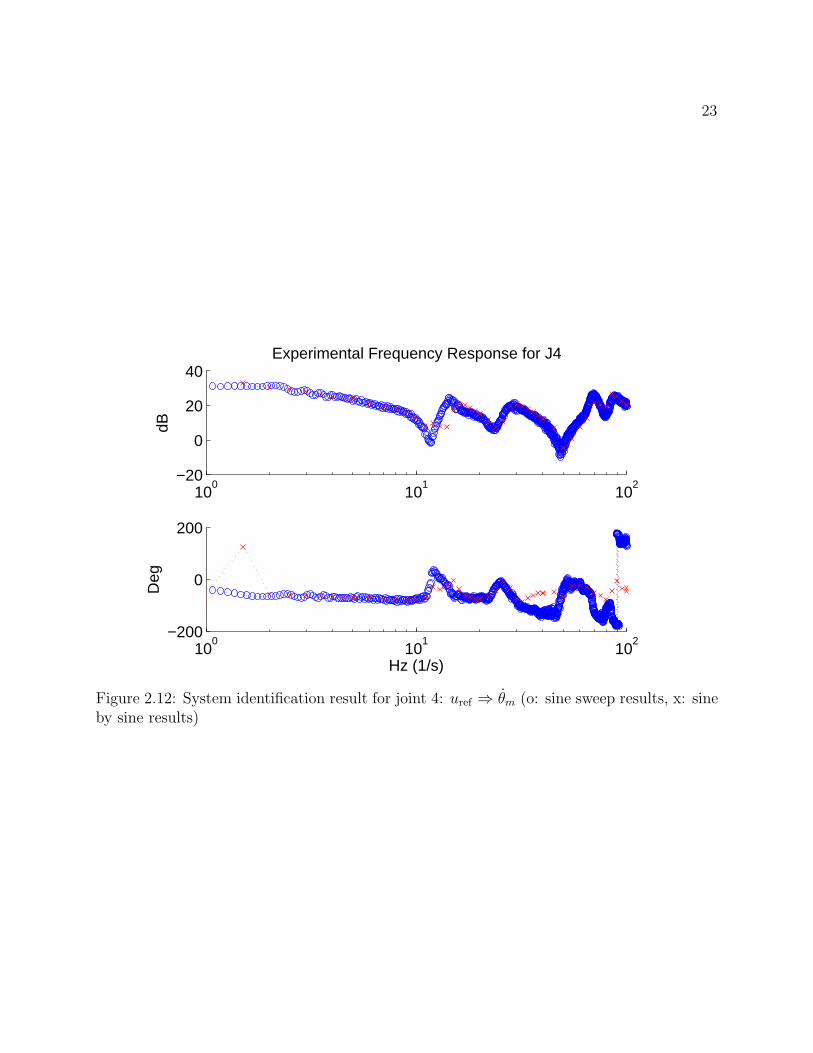
2.12 System identification result for joint 4: uref ⇒ θm (o: sine sweep results, x: sineby sine results) . . . . . . . . . . . . . . . . . . . . . . . . . . . . . . . . . . . . 23



3.1 Block diagram of procedure to obtain ∇J(xk) . . . . . . . . . . . . . . . . . . . 283.2 Frequency response of bandpass filter centered at 0.29π with b = 0.1 . . . . . . . 293.3 Plots of B1(xk) and B2(xk) on the top and bottom respectively . . . . . . . . . 333.4 Logic tree for selecting nk . . . . . . . . . . . . . . . . . . . . . . . . . . . . . . 373.5 Feedback controller structure for an individual joint . . . . . . . . . . . . . . . . 383.6 System identification result for joint 4 (Blue circles indicate the measured fre-

quency response from a sine sweep, black crosses indicates the response of anideal first order model) . . . . . . . . . . . . . . . . . . . . . . . . . . . . . . . . 39

3.7 System identification result for joint 5 (Blue circles indicate the measured fre-quency response from a sine sweep, black crosses indicates the response of anideal first order model) . . . . . . . . . . . . . . . . . . . . . . . . . . . . . . . . 40

3.8 System identification result for joint 6 (Blue circles indicate the measured fre-quency response from a sine sweep, black crosses indicates the response of anideal first order model) . . . . . . . . . . . . . . . . . . . . . . . . . . . . . . . . 41

3.9 Cost function versus iteration while tuning J1 of the FANUC M-16iB robot . . 453.10 Cost function versus iteration while tuning J2 of the FANUC M-16iB robot . . 463.11 Cost function versus iteration while tuning J3 of the FANUC M-16iB robot . . 473.12 Cost function versus iteration while tuning J4 of the FANUC M-16iB robot . . 483.13 Cost function versus iteration while tuning J5 of the FANUC M-16iB robot . . 493.14 Cost function versus iteration while tuning J6 of the FANUC M-16iB robot . . 50

4.1 Typical DOB structure . . . . . . . . . . . . . . . . . . . . . . . . . . . . . . . . 524.2 Parallel controller structure . . . . . . . . . . . . . . . . . . . . . . . . . . . . . 534.3 Proposed DOB framework for controller tuning . . . . . . . . . . . . . . . . . . 544.4 Equivalent representation of Fig. 4.3 for stability analysis . . . . . . . . . . . . . 544.5 Block diagram representation of GEU as a structured uncertainty problem . . . 554.6 Nyquist plot of C(s)G(s) . . . . . . . . . . . . . . . . . . . . . . . . . . . . . . . 57

5.1 Two inertial model of an indirect drive mechanism . . . . . . . . . . . . . . . . 635.2 Single mass simplification . . . . . . . . . . . . . . . . . . . . . . . . . . . . . . 645.3 Nominal step response of a second order system . . . . . . . . . . . . . . . . . . 665.4 Motor side step response tracking . . . . . . . . . . . . . . . . . . . . . . . . . . 685.5 Load side step response . . . . . . . . . . . . . . . . . . . . . . . . . . . . . . . 695.6 Load side step response comparison . . . . . . . . . . . . . . . . . . . . . . . . . 70

v

5.7 Trajectory correction: top subplot shows the original desired load side trajectory,bottom subplot shows the trajectory correction, δθd,l . . . . . . . . . . . . . . . 71

5.8 Compensated response: top subplot shows the load side tracking performance,bottom subplot shows load side error . . . . . . . . . . . . . . . . . . . . . . . . 72

5.9 Compensated response: top subplot shows the load side tracking performance,bottom subplot shows load side error (90 % of default inertia) . . . . . . . . . . 73

5.10 Compensated response: top subplot shows the load side tracking performance,bottom subplot shows load side error (50 % of default inertia) . . . . . . . . . . 74

5.11 Compensated response: top subplot shows the load side tracking performance,bottom subplot shows load side error (200 % of default inertia) . . . . . . . . . 75

5.12 System identification posture for first 3 joints of the FANUC M-16iB robot . . . 755.13 Load side acceleration response used for system identification of joint 1 . . . . . 765.14 Load side acceleration response used for system identification of joint 2 . . . . . 765.15 Load side acceleration response used for system identification of joint 3 . . . . . 775.16 Compensated response: top subplot shows the load side position tracking perfor-

mance, bottom subplot shows load side error . . . . . . . . . . . . . . . . . . . . 775.17 Compensated response: load side position tracking error along X axis . . . . . . 785.18 Compensated response: load side position tracking error along Y axis . . . . . . 785.19 Compensated response: load side position tracking error along Z axis . . . . . . 79

List of Tables

2.1 Feedback parameters for system identification . . . . . . . . . . . . . . . . . . . 17

3.1 Parameters for gain tuning . . . . . . . . . . . . . . . . . . . . . . . . . . . . . . 44

4.1 Verified stable gain variations in DOB framework through simulation . . . . . . 604.2 Verified stable gain variations in DOB framework through experimentation . . . 60

vi

Acknowledgments

This dissertation is a culmination of 5 years of hard work at the University of California,Berkeley. But needless to say, this dissertation would probably not have been written if itwere not for the people in my life supporting me these past years. First and foremost, I wouldlike thank Professor Tomizuka for initially taking me in as his student back in 2009. Underhis guidance, I have learned much in the area of control theory and mechatronics. But moreimportantly, Professor Tomizuka gave me an opportunity to learn how complicated graduatelevel research can be. It was definitely a humbling experience to realize how little I kneweven after completing college. Additionally, I would also like to thank Professor Tomizuka’swife, Miwako sensei, for always being such a cheerful host whenever Professor Tomizukawould throw a party at his home.

I would also like to thank FANUC Corporation for supporting my research these past 5years. In particular, I would like to personally thank Dr. Seiuemon Inaba, Dr. YoshiharuInaba, and Dr. Kiyonori Inaba for their continued support and confidence in the MechanicalSystems Controls (MSC) Laboratory at the University of California, Berkeley. I hope that thecontinued collaboration between FANUC and Berkeley will continue to produce invaluabletechnologies for FANUC Corporation.

At this point I would also like to thank my family for their continued support these pastfew years. In particular, I would like to thank my dad and mom, Pak and Ming, for post-poning their retirement for a few years as I toiled away in graduate school. My grandparentsfor always making home a welcoming place whenever I returned for the holidays. And mybrother, Alan, for taking care of things at home while I was away for graduate school.

I would also like to thank the many individuals I met while studying at Berkeley. Iwould to thank Shih-Yuan, Chi-Shen, Oak, Max, Selina, and Raechel for your friendshipand for being an excellent source of entertainment and amusement during both the goodtimes and the bad. In particular, a special shout out to Shih-Yuan and Chi-Shen for invitingme out to the BATS events early during my graduate studies, thus giving me somewhatof a resemblance of a social life in graduate school. I would also like to give my thanks tothe other members of the robotics research group, namely Nora, Wenjie, Pedro, Cong, andChung-Yen. It was a pleasure exchanging intellectual thoughts with you guys (and girl) thesepast years. I would also like to give my thanks to the remaining individuals in ProfessorTomizuka’s research lab: (Current members) Chen-Yu, Yaoqiong, Kevin, ChangLiu, Junkai,Robert, Dennis, Yizhou, Xiaowen, Wenlong, (Alumni) Evan, Sanggyum, Joonbum, Nancy,Emma, Hoday, Haifei, Lucy, Steve, KC, Takashi, Steve, Ben, Hiroshi, Omar, Kengo, James,and William. I was able to learn a lot about doing research in fields other than my own dueto my interactions with you all and listening to your weekly research seminars. In addition,I would also thank Sugi-san for his technical guidance and friendship while he was still herein Berkeley. I hope to keep in touch and I wish you all the best in your future endeavors.

1

Chapter 1

Introduction

1.1 Background

Feedback control is often an under appreciated concept. Most human beings, given theirsensitive, yet robust, senses of vision, hearing, touch are capable of doing many miraculousfeats. Yet even the simplest of feats, such as walking or catching a ball, would not bepossible if it was not for the constant visual, audio, and tactile feedback the human bodyprovides to the brain. The brain can process this information which then allows the humanto react and, in some cases, anticipate events. This latter concept is called feedforwardcontrol by people in the Controls community. Yet despite all the advantages that feedbackand feedforward control provides, humanity rarely acknowledges these concepts outside ofthe Controls community.

Similarly, industrial automation is also an under appreciated field in robotics. Roboticshas always stemmed from humanity’s desire to create life. Even the term ’robot’ was firstcoined by the Russian science fiction writer Isaac Asimov when he was envisioning a worldwith robots that were human-like in appearance. As a result, the general public tends toassociate robots with androids and other human-like robots. But in reality, the vast majorityof the robots today are fixed industrial machines that are not human-like in appearance atall. But more importantly, these industrial machines play a crucial role in the advancementof a nation’s manufacturing capabilities.

This dissertation in return focuses on these two under appreciated concepts. More specif-ically, this dissertation will talk about how fundamental principles such as feedback andfeedforward control can be further refined to improve the performance of industrial robots.

1.2 Motivation and Contribution

In today’s competitive manufacturing environment, industrial robots are pushed to operatenear their designed hardware and software limitations. Even so, manufacturers still demand

2

more performance from their machinery. Rather than redesigning the hardware for theseindustrial robots, which is a costly strategy, an alternative is to design better software algo-rithms. This dissertation focuses primarily on the software aspect by introducing intelligentcontrol algorithms that can improve the performance of industrial manipulators.

This dissertation can be roughly divided into two sections. The first two-thirds of thedissertation focuses on feedback techniques while the last third of the dissertation will em-phasize feedforward techniques. In the feedback portion, the dissertation presents a novelapplication of extremum seeking control (ESC) for use with industrial robotics as well aspresent a novel platform based off the disturbance observer (DOB) which can be appliedfor gain tuning applications. In the feedforward portion, a simple input shaping methodis demonstrated to work efficiently at reducing transient vibrations in flexible joint robots.While the feedback and feedforward techniques in this dissertation can be used in unison,they are implemented individually in this dissertation for the purpose of demonstrating theeffectiveness of each approach.

Sensor-based Feedback Controller Tuning of Robot Manipulatorsby Nonlinear Programming

In current practice, whenever a new robot model is introduced, experienced engineers haveto spend a long period of time to tune and validate the feedback and feedforward controllergains for the robot. This process is performed on a single robot and then applied to allother robots of the same model. As a result, these tuned gains have to be robust to bothmanufacturing uncertainties and different robot applications. Furthermore, robot dynamicsare highly nonlinear and can vary substantially from one configuration to another. While itis possible to use a fixed set of gains to stabilize a robot for its entire workspace, it is highlyunlikely that these controller gains can guarantee good performance for any given trajectoryin the workspace. Hence in an industrial setting, the ability to quickly optimize the robotcontroller for any particular task can likely improve robot performance. Manually retuningrobots can be a time consuming and expensive process. Hence it is desirable to have analgorithm that can automatically tune robot controllers based on a user specified trajectory.Chapter 3 focuses on the development of an automated gain tuning algorithm for industrialmanipulators.

A Disturbance Observer Framework for Stable FeedbackController Tuning

Feedback control is essential for good performance in almost any electro mechanical system.Consequently, a great deal of effort is put into properly designing feedback controllers. Themost practical controller used in industrial robots today is still the proportional plus integralplus derivative (PID) controller. The PID controller has many practical properties that make

3

them easy to tune and use, namely, the controller parameters have very intuitive physicalimplications which makes manual tuning feasible. As computational technologies improve,however, it may be possible to take advantage of more advanced higher order controllers tofurther improve robot performance. Tuning these higher order controllers, however, may notbe as intuitive as tuning a PID controller. An alternative method is to empirically tune thesehigher order controllers using a nonlinear programming technique. This approach, however,may run into stability issues as higher order controllers are more likely to excite a system’shigher order dynamics. Chapter 4 focuses on developing a gain tuning framework that isrobustly closed loop stable for controller tuning applications.

An Input Shaping Method to Suppress Transient Vibrations InFlexible Joint Robotic Manipulators

Actuators found in mechanical systems have to satisfy a variety of seemingly conflictingrequirements. Often these actuators are required to have high positioning accuracy, goodrepeatability, and high torque capacity while simultaneously required to be compact, light,and competitively priced. To meet these demands, engineers decide to introduce various gearreduction mechanisms (also called transmission) between the motor output and the actualoutput shaft of the actuator. This way, a light and high speed motor with low torque capacityand moderate positioning accuracy can be used to transmit large amounts of torque with highpositioning accuracy. Systems that utilize this actuator and transmission setup are calledindirect drive mechanisms. Although they have many benefits, indirect drive mechanismsalso create interesting problems for control engineers. Namely, the transmission mechanismhas its own dynamic properties. For a variety of reasons, the sensors used for motor feedbackare usually placed prior to the transmission mechanism, hence a good feedback controllerthat provides excellent motor performance cannot guarantee good performance of the out-put shaft of the actuator. If the transmission dynamics are known, however, feedforwardtechniques can be used to shape the desired motor reference trajectory to pre-compensatefor the transmission dynamics. Chapter 5 focuses on developing an input shaping approachto compensate for the dynamics of a particular family of transmission mechanisms, namelystrain wave gearing mechanisms.

1.3 Dissertation Outline

The remainder of this dissertation is organized as follows: Chapter 2 will introduce basicrobotics and system modeling ideas used throughout this dissertation. Additionally, thechapter will also detail the experimental setup used to verify the developed algorithms inthis dissertation. Chapter 3 will introduce an automatic controller tuning algorithm basedon nonlinear programming. This chapter will also provide methods of selecting importantparameters such as initial controller gains and stepsizes. Chapter 4 will introduce a frame-

4

work based on the disturbance observer (DOB) concept that can be used for tuning higherorder controllers. The chapter will also prove that the framework is robustly stable given afew mild constraints. Chapter 5 will introduce an input shaping technique to compensatefor transmission dynamics. A simple procedure for empirically identifying the transmissionparameters will also be introduced. And finally, the main results and contributions of thisdissertation will be highlighted in Chapter 6. Additionally, this chapter will also discusspossible extensions for the work presented in this dissertation.

5

Chapter 2

System Modeling, HardwareDescription, and System Identification

2.1 Introduction

This chapter summarizes all the modeling, hardware, and system identification results neces-sary to understand the remainder of this dissertation. Section 2.2 motivates and introducesthe two mass model used for studying indirect drive mechanisms. In particular, this sectionwill also highlight the modeling simplifications used in this dissertation due to the nature ofindustrial robotic manipulators. Section 2.3 briefly introduces the dynamics for a 6 degreeof freedom (DOF) robotic manipulator. Section 2.4 talks about both the physical hardwareand simulation software that is used to verify the theory presented in the later chaptersof this dissertation. Section 2.5 highlights the system identification process used to obtainempirical frequency response data for the physical hardware. And finally, the contents ofthis chapter will be summarized in section 2.6.

2.2 Two Mass Model

Given the physical nature of indirect drive mechanisms, many researchers chose to use atwo inertia model to physically model the behavior of the indirect drive mechanism [39,16, 23]. This two inertial model is shown in Fig. 2.1. J∗ and θ∗ denote the inertia anddisplacement. The subscripts m and l denote the motor side and load side parametersrespectively. In the proposed model, the torque input, u, is applied on the motor side.Furthermore, motor side viscous damping is captured by the viscous damping coefficient,dm, whereas the other motor side nonlinear forces and damping effects are denoted generallyas fnl,m. The transmission is modeled as a combination of a linear spring and viscous damper,whose coefficients are denoted by kj and dj respectively, as well as nonlinear joint frictionforces and joint transmission error denoted by fnl,j and θ respectively. Also note that the

6

transmission mechanism also reduces the displacement from the motor side to load side bya factor of N . The transmission error, θ is defined as the deviation between the expectedoutput position and the actual output position. More specifically, it is given as:

θ =θmN

− θl (2.1)

The behavior of the transmission error depends heavily on the transmission mechanism itself.The transmission error will be addressed more specifically later in this chapter. Looking backat the two inertial model, performing a torque balance on the two inertia elements in Fig. 2.1yields:

Jmθm = −dmθm − kjN

(θmN

− θl − θ)− dj

N

(θmN

− θl − ˙θ)− fnl,m − fnl,j + u

Jlθl = −kj

(θl − θm

N+ θ

)− dj

(θl − θm

N+ ˙θ

) (2.2)

Note that the motor side and load side displacements, velocities, and accelerations are cou-pled together in Eq. (2.2). Furthermore, if the nonlinear friction effects and transmissionerror are ignored, the ideal relationship between the motor input and motor position as wellas load position in the Laplace domain is given by:

Gmu(s) =θm(s)

u(s)=

Jls2 + djs+ kj

JmJls4 + Jds3 + Jks2 + kjdms(2.3)

Glu(s) =θl(s)

u(s)=

djs+ kjN (JmJls4 + Jds3 + Jks2 + kjdms)

(2.4)

where:

Jd = Jmdj + Jl

(djN2

+ dm

)(2.5)

Jk = Jmkj +JlkjN2

+ djdm (2.6)

Other relevant transfer function variants for the two inertia system are:

Gdmu(s) =θm(s)

u(s)=

Jls2 + djs+ kj

JmJls3 + Jds2 + Jks+ kjdm(2.7)

Gddlu(s) =θl(s)

u(s)=

djs2 + kjs

N (JmJls3 + Jds2 + Jks+ kjdm)(2.8)

Transmissions for Industrial Manipulators

Flexible gear reducers are commonly used in industrial robots due to their high gear reduc-tion ratios [33]. Among the different types of flexible gear reducers, the discussion in this

7

u θm

Jm

dm

fnl,m

dj

kj

N , θ, fnl,j

Jl

θl

��

��

Figure 2.1: Two inertial model of an indirect drive mechanism

subsection will focus harmonic drives since variants of their transmission properties can befound in many of the other reducers used in industrial robots. The main components ofa harmonic drive are identified in Fig. 2.2 [21]. The wave generator is a rigid core havingan slightly elliptical shape. The wave generator fits inside the flexspline, which is usually athin-walled hollow cup. The teeth of the flexspline are on the outside surface of the hollowcup and the output of the harmonic drive is also attached to the flexspline. The flexsplinefits inside the circular spline. The circular spline is a rigid and fixed component that hasteeth machined along the inside surface. Usually, there are two fewer teeth along the outsideof the flexspline as there are along the inside of the circular spline. This difference in teethcauses the flexspline to essentially rotate by the difference in teeth for every full rotationof the wave generator. This design allow harmonic drives to efficiently achieve large gearreduction ratios. Additionally, the inherent multiple-tooth contact design in harmonic drivesalso allow them to withstand high amounts of torque while simultaneously eliminating alltransmission backlash [38]. Additional advantageous properties of harmonic drives include:lightweight and compact design, high efficiency, and backdrivability.

The harmonic drive, however, is not without its disadvantages. The use of the flexsplinein the harmonic drive instills a large amount of flexibility in the drive. Additionally theconcentric nature of the harmonic drive assembly tend to give rise to kinematic errors dueto manufacturing and alignment inaccuracies. Studies show that these kinematic errors

8

Figure 2.2: Harmonic drive components

occur dominantly at a frequency of twice the wave generator rotation velocity. The rootcause of these kinematic errors are caused by manufacturing and assembly imperfections inthe harmonic drive. More specifically, the tooth placement errors along the flexspline andcircular spline as well as misalignment of the three major harmonic drive components [38].In this dissertation, the kinematic errors caused by component misalignment, manufacturing

9

imperfections, and nonlinear flexspline flexibilities are denoted as the transmission error θ.Additionally the nonlinear friction effect caused by the meshing of the flexspline and circularspline is denoted by fnl,j whereas the linear flexibility and damping effects are characterizedby the linear joint stiffness and damping coefficients kj and dj respectively.

Much work has been done on trying to compensate for the transmission error and non-linear friction effects found in harmonic drives [20, 17, 8]. As a result, the work in thisdissertation will not focus on the transmission error or nonlinear friction effects, but insteadwill focus primarily on compensating for the linear flexibilities and damping. For all inten-sive purposes, the nonlinear friction effects and transmission error will be treated as processnoise or disturbances in this dissertation.

2.3 Multiple Degree of Freedom Robot Model

This dissertation will only consider serial industrial manipulators. The dynamics of a nDOF serial industrial manipulator with joint flexibilities can be derived through Lagrangiandynamics and can be expressed generally as:

Ml(ql)ql + C(ql, ql)ql +G(ql) +Dlql + Flcsgn(ql) + J(ql)Tfext

= Kj (N−1qm − ql − q) +Dj

(N−1qm − ql − ˙q

) (2.9)

Mmqm +Dmqm + Fmcsgn(qm) =τm −N−1 [Kj (N

−1qm − ql − q) +Dj (N−1qm − ql − q)]

(2.10)

where ql ∈ Rn and qm ∈ Rn denote the load side and motor side position vectors where theith element denote the position at the ith joint. q ∈ Rn is the vector of transmission errorscaused by flexible joint reducers. M∗ ∈ Rn×n, D∗ ∈ Rn×n, and F∗c ∈ Rn×n are the inertia,viscous damping, and coulomb friction matrices respectively. Again the subscripts l and mdenote load side and motor side respectively. C(ql, ql) ∈ Rn×n is the Coriolis and centrifugalforce matrix, G(ql) ∈ Rn is the gravity torque vector, N ∈ Rn×n is the matrix containing thegear reduction ratios of each reducer, and J(ql) ∈ R6×n is the Jacobian matrix which mapsthe load side joint space to the end-effector Cartesian space. Kj ∈ Rn×n and Dj ∈ Rn×n

are the joint linear stiffness and viscous damping matrices respectively. Vectors τ ∈ Rn andfext ∈ R6 denote the motor input torques and external forces/torques acting on the robotend-effector in the Cartesian coordinate system. Note that Mm, Kj, Dj, Dl, Dm, Flc, Fmc,and N are all diagonal matrices.

In the case where the joints are rigid, Eqs. (2.9-2.10) can be combined and rewritten as:

M(q)q + C(q, q)q +G(q) +Dq + Fcsgn(q) + J(q)Tfext = τ (2.11)

where q = ql, τ = Nτm, M(q) = Ml(ql) + N2Mm, C(q, q) = C(ql, ql), D = Dl + N2Dm,Fc = Flc +NFmc, and J(q) = J(ql).

10

Decentralized Analysis

In general, it is difficult to analyze and design control algorithms for the coupled multiple-input-multiple-output (MIMO) system described by Eq. (2.9-2.10). More specifically, theinertia, gravity, external, Coriolis, and centrifugal forces cause the behavior at each individualjoint to be coupled with each other. This coupling is characterized by the off diagonal termsin the corresponding matrices. In many cases, however, the diagonal terms in these matricesare substantially larger than those in the off diagonal terms. While the coupling effects arenon-negligible, this dissertation will mainly treat the analysis of each joint in a multipledegree of freedom robot as essentially decoupled. The coupling effects will be regarded asregular process noise. Although this is a nontrivial assumption, the developed algorithms inthis dissertation will be experimentally validated. The experimental results will shed lighton the limitations caused by this assumption.

2.4 Hardware and Software Setup

As mentioned in the previous section, all the developed algorithms in this dissertation areexperimentally verified. The FANUC M-16iB [14] industrial manipulator, provided to theUniversity of California, Berkeley, by FANUC Corporation, is used for all the experimentalverifications in this dissertation. This setup is shown in Fig. 2.3. The FANUC M-16iB is astandard 6-DOF serial industrial manipulator with a 20 kg payload capacity. The namingand positive rotation conventions for each joint of the FANUC M-16iB robot is depicted inFig. 2.4. Each joint of the robot uses a gear reduction mechanism. Due to the high inertialoads on the first three joints (J1-J3), the joint flexibilities in these joints are dominantcompared to those on the last three joints (J4-J6). As a result, this dissertation will focuson the joint flexibilities of J1-J3 only whereas J4-J6 are assumed to be rigid. The first threejoints of the robot uses Rotor-Vector (RV) reducers [34]. RV reducers contains elements ofboth a planetary gearbox and a harmonic drive. The RV reducer design allows it to keepmost of the strengths and weakness found in a harmonic drive. One noticeable difference isthat the dominant kinematic error in RV reducers occurs at a frequency that is eight timesthat of the wave generator rotation frequency.

For sensing, the FANUC robot is equipped with motor side encoders at each joint. Theseencoders are standard on the commercially available M-16iB and provide the motor positionand velocity information for feedback. In addition to the motor encoders, an inertia sensor(Analog Devices, ADIS16400) [1] has also been attached to the end-effector to provide threedimensional end-effector angular velocity and translational acceleration measurements. Thethree dimensional end-effector position can also be measured with the CompuGauge 3D [12].If direct contact to the robot end-effector is not desirable, then a Position Sensitive Detector(PSD) [11], also referred to as the PSD camera, can be utilized to obtain the end-effectorposition measurements. In this dissertation, only the motor encoders are used for real-time

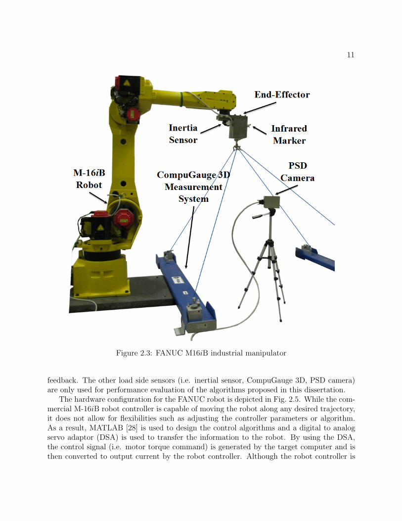
11

Figure 2.3: FANUC M16iB industrial manipulator

feedback. The other load side sensors (i.e. inertial sensor, CompuGauge 3D, PSD camera)are only used for performance evaluation of the algorithms proposed in this dissertation.

The hardware configuration for the FANUC robot is depicted in Fig. 2.5. While the com-mercial M-16iB robot controller is capable of moving the robot along any desired trajectory,it does not allow for flexibilities such as adjusting the controller parameters or algorithm.As a result, MATLAB [28] is used to design the control algorithms and a digital to analogservo adaptor (DSA) is used to transfer the information to the robot. By using the DSA,the control signal (i.e. motor torque command) is generated by the target computer and isthen converted to output current by the robot controller. Although the robot controller is

12

��

��

��

��

��

Figure 2.4: Joint naming and rotating conventions for the FANUC M16iB robot

not directly generating signals to control the robot, it is still used to amplify the output fromthe target computer. In addition, the robot controller is also used to activate the mechanicalmotor brakes in the robot. Note that the brake function is turned on and off directly witha digital input/output (DIO) board installed on the target computer.

In operating real-time systems such as the FANUC robot using MATLAB, it is criticalthat computational hardware performance runs as quickly and as consistently as possible.More specifically, it is important that the hardware performance of the robot is not limitedby computational limitations from the computer used for control. Since MATLAB runs on aWindows platform, it is not guaranteed that the real-time computation will not be hinderedby virus scanning software and other event logging processes. To overcome this problem,two computers are used for the real-time control system setup. A host computer runningWindows and MATLAB is used to design and implement the algorithms in this disserta-

13

��

��

��

��

� � �� !��" �� #��"

��

$ % �� ""��&��#%�!

'��"�#�#(

��

� � ��

��

��) ��

��*% �

'��

��'��+,,

� -)�.��/�

��-��

�0��-

�'��.�

��-��

��

&��#%�!'��"�#�#(

��)��#��"��"'�)��12��)��'�,3/��4�� #��"��5 �#)��

Figure 2.5: FANUC M16iB robot system setup scheme

tion. Once the design and coding for the algorithms are complete on the host computer, theinformation is then compiled and loaded onto the second computer via an ethernet connec-tion. This second computer, also called the target computer, runs the MATLAB XPCtargetenvironment. The XPCtarget environment allows the target computer to execute the com-piled information from the host computer. Once the target computer begins running thecontrol algorithm, the connection between the two computers is automatically disengaged,thus allowing the target computer to run without any interferences from the host computer.The current minimum sampling time for the XPCtarget is 0.5 msec. Additionally, the robotencoder information is accessible by the target computer through a high-speed serial bus(HSSB) interface while the inertia sensor information is acquired through an National In-struments (NI) FPGA board.

In addition to the aforementioned hardware a simulator is also available for the FANUCM-16iB robot. The simulator is mainly constructed in the MATLAB Simulink environmentand utilizes both the SimMechanics and Robotics toolbox [13]. This simulator is capable of

14

simulating the dynamic behaviors of the robot. Preliminary studies show that the behaviorof the physical robot system can be captured by the robot simulator model. As a result, therobot simulator is used to test the proposed algorithms in this dissertation prior to actualimplementation on the FANUC M-16iB robot.

Controller Structure

By default, the FANUC M-16iB robot uses a decentralized PID feedback controller scheme.The block diagram for a single joint of the robot is depicted in Fig. 2.6. The controller consistsof two loops, an inner velocity feedback loop and an outer position feedback loop. The innerloop is controlled with a Proportional plus Integral (PI) controller with parameters Kv andKi respectively whereas the outer loop is controlled with a simple Proportional controllerwith parameter Kp [15]. Combining the two loops together, the resulting feedback controlleris a Proportional-Integral-Derivative (PID) controller whose transfer function from the motorposition error, e = θm,ref − θm, to the feedback torque, ufb, is given by:

C(s) =ufb(s)

e(s)=

Kvs2 + (KpKv +Ki) s+KpKi

s(2.12)

The feedforward torque, uff is computed using a recursive algorithm that solves the Newton-Euler equations for the robot [35] and is represented simply as just F2 block in Fig. 2.6. Notethat the Newton-Euler equations are solved in a centralized manner, hence all the referencejoint trajectories are needed. This aspect is not depicted in Fig. 2.6. The algorithm isimplemented via the robotics toolbox mentioned earlier. The feedforward torque calculationrequires the desired robot joint trajectory to be entirely known in advance. Although thealgorithm for computing the feedforward torque is recursive, it is extremely computationallyintensive and cannot be computed in real time. The computed feedforward torque using thisapproach, however, is extremely accurate and provides the majority of the performance forthe robot manipulator. The primary role of the feedback controller then is to compensate forany residual errors that is not captured by the recursive Newton-Euler (RNE) feedforwardtorque. Since most of the time, it is more convenient to define the robot’s trajectory fromthe load side perspective, the feedforward block F1 is a conversion between the desired loadside trajectory, θl,ref , to the desired motor side trajectory, θm,ref . In many cases, F2 is simplya multiplication by the respective gear ratio N .

2.5 System Identification

As mentioned in Section 2.3, each joint of the 6 DOF industrial robot will be analyzed ina decoupled manner. In this decoupled analysis, a single two inertia model as described inFig. 2.1 is used to represent the dynamic behavior of each joint. As with all models, thetwo inertia model is a simplified model that cannot capture all the dynamics of the physical

15

θl,refKp

−

∫

+

−

+ Kv

Ki

+

d

dt

��

� ��θm

θm,ref

uff

d

dt

e

+

ufb

θl

F1

F2

Figure 2.6: Decentralized feedback controller scheme

system. Hence a system identification on the physical FANUC M-16iB robot is performed tomeasure the actual dynamic behavior of the robot. This data is useful for both identifyingsome of the model parameters and also learning the bandwidth limitations of the two inertiamodel.

The system identification was performed one joint at a time. Two different systemidentification experiments were performed for each joint. The first is a sine sweep experimentwhich harmonically excites the joint from 1 Hz to 100 Hz over a 180 second span. Theobjective of the sine sweep experiment is to capture an initial estimate of the joint frequencyresponse. The second experiment is a sine by sine test. In the sine by sine test, the joint isexcited at a particular frequency for a fixed amount of time, stops, and then proceeds to thenext excitation frequency. The sine by sine experiment provide a more accurate frequencyresponse than the sine sweep experiment since the excitation frequency is stationary at eachfrequency. In addition, the sine by sine gives the user more flexibility in setting testingparameters such as the experimental time duration spent exciting each frequency. This isimportant as lower excitation frequencies require a longer excitation duration to acquiremeaningful data. For each system identification experiment, three measurements: motorposition, θm, motor velocity, θm, and load acceleration, θl are recorded. The control structurefor the system identification process is shown in Fig. 2.7. During the system identificationprocess, the reference trajectory for each joint is set to zero and the feedforward torque, uff ,is used for gravity compensation only. The sinusoidal torque, uref is injected at the samepoint as the feedforward torque. Since the reference trajectory is set to zero at every joint,the feedback controller, C(s), may produce conflicting torque commands at the joint that isundergoing system identification. As such, the gains of C(s) for the joint being identified isset to be substantially lower to reduce the feedback controller effects. More specifically, the

16

Kp−

∫

+

−

+ Kv

Ki

+

d

dt

��

� ��θm

θm,ref

uff + uref

d

dt

+

ufbe

C(s)

G(s)

θl

Figure 2.7: Controller for system identification

closed loop transfer function in Fig. 2.7 can be expressed as:

θmuref

=G(s)

1 +G(s)C(s)(2.13)

Hence by selecting the gains, Kp, Kv, and Ki to be very small, G(s)C(s) ≪ 1 and theeffect of the feedback controller can be neglected. For joints that are not heavily influencedby gravity effects, the controller gains can be set exactly to zero. But non-zero feedbackcontroller gains are necessary to maintain safe robot motions during the system identificationprocess otherwise. In all experiments and for all joints, the integrator gain, Ki, is set to zero.The remaining controller controller gains used for each joint during the system identificationprocess for each joint are tabulated in Table 2.1. Additionally, the posture of the FANUCM-16iB robot during the system identification process for each joint is shown in Fig. 2.8.

Parameter Identification

Much of the postprocessing of the measured data is done through the MATLAB’s SystemIdentification Toolbox. The processing accepts the input torque command and measuredoutput data as an input and returns the estimated magnitude and phase for this input-output relationship at each measured frequency. Ideally the system identification should beperformed in an open loop manner. But as mentioned in the previous section, small feedbackgains are used to keep the robot system stable during the experiment due to gravity effects.But since the structure of the feedback controller and the gain values are known, it is possibleto calculate the open loop transfer function from the estimated closed loop data. The firststep to doing so is to convert the magnitude and phase estimates into the real and imaginaryparts of the closed loop transfer function. Consider a closed loop transfer function:

Gcl(jω) = α(ω) + jβ(ω) (2.14)

17

Table 2.1: Feedback parameters for system identification

Joint ID Joint Feedback GainsJ1 J2 J3 J4 J5 J6

J1 Kp 0 10 10 20 20 20Kv 0 0.2280 0.05072 0.08592 0.0046 0.003986

J2 Kp 10 5 10 20 20 20Kv 0.1533 0.1 0.05072 0.08592 0.0046 0.003986

J3 Kp 10 10 2 20 20 20Kv 0.1533 0.2280 0.01 0.08592 0.0046 0.003986

J4 Kp 10 10 10 0 20 20Kv 0.1533 0.2280 0.05072 0 0.0046 0.003986

J5 Kp 10 10 10 20 0 20Kv 0.1533 0.2280 0.05072 0.08592 0 0.003986

J6 Kp 10 10 10 20 20 0Kv 0.1533 0.2280 0.05072 0.08592 0.0046 0

where α(ω) ∈ R and β(ω) ∈ R represents the coefficients of the real and imaginary part ofthe closed loop transfer function, Gcl, evaluated at frequency ω. The magnitude and phaseof the closed loop transfer function can be represented as:

|Gcl(ω)| =√α2(ω) + β2(ω) (2.15)

∠Gcl(ω) = tan−1(β(w)

α(w)) (2.16)

With some algebraic manipulation, the coefficients α(ω) and β(ω) can be expressed as:

β(ω) = α(ω) tan(∠Gcl(ω)) (2.17)

α(ω) =

√|Gcl(ω)|2

1 + tan2(∠Gcl(ω))(2.18)

Due to the inherent nature of tan(·), one needs to be careful when assigning the signs forα(ω) and β(ω) using Eqs. (2.17-2.18). Once the coefficients are calculated, one can deducethe real and imaginary parts of G(jω) by equating the real and imaginary parts of Gcl(jω)and utilizing Eq. (2.13). More specifically, one can define the following:

C(jω) = σ(ω) + jγ(ω) (2.19)

G(jω) = x(ω) + jy(ω) (2.20)

Combining Eq. (2.14), (2.19), and (2.20) with Eq. (2.13) and equating the real and imaginaryparts on both sides of the equations yield two equations and two unknowns, namely x(ω) and

18

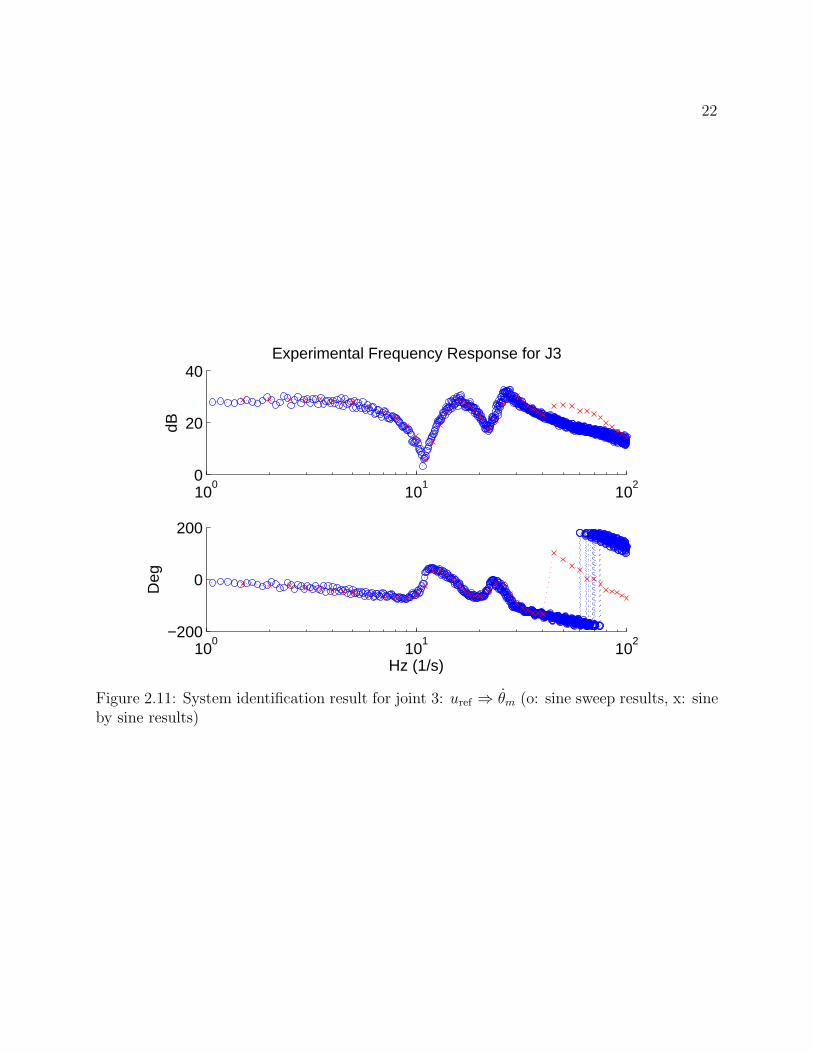
y(ω). Note that since the controller structure and gains are known, σ(ω) and γ(ω) can becomputed. The bode plots of the system identification results from the motor input torque,u/rmref to motor velocity, θm, are shown in Figs 2.9-2.14. The blue circles indicate the sinesweep results whereas the red crosses indicate the sine by sine results. Note that at lowfrequencies, both the sine sweep and sine by sine results are closely matched. Furthermore,the system identification results suggest that the first three joints (J1-J3) have much simplerthan dynamic behavior than the three wrist joints (J4-J6) of the FANUC robot. Also notethat the first three joints have a clear antiresonance and resonance behavior at about the 10Hz range. This dynamic behavior can be captured by the two mass model relationship givenin Eq. (2.7). The parameter identification and transfer function fitting process is detailed inlater relevant chapters.

2.6 Chapter Summary

This chapter introduced the two inertia model used to model indirect drive mechanisms.The chapter also talked about typical transmission used in industrial robots. In particular,the harmonic drive was discussed in detail in Section 2.2. Then the dynamic equations of amulti DOF robot was briefly introduced. A few modeling assumptions and their justificationswere also discussed. The chapter then talked about the hardware and software configurationused when producing the results in this paper. Finally, the chapter closed by discussing thesystem identification process used to identify and characterize the actual hardware behavior.The material in this chapter is a necessary prerequisite to understanding the later chaptersof this dissertation.

19

J1

J2

J4

J5

J3 J6

Figure 2.8: Robot postures for system identification

20

100

101

102

−20

0

20

40Experimental Frequency Response for J1

dB

100

101

102

−200

0

200

Deg

Hz (1/s)

Figure 2.9: System identification result for joint 1: uref ⇒ θm (o: sine sweep results, x: sineby sine results)

21

100

101

102

−20

0

20


dB

100

101

102

−200

0

200

Deg

Hz (1/s)


22

100

101

102

0

20


dB

100

101

102

−200

0

200

Deg

Hz (1/s)


23

100

101

102

−20

0

20


dB

100

101

102

−200

0

200

Deg

Hz (1/s)


24

100

101

102

−50

0

50


dB

100

101

102

−200

0

200

Deg

Hz (1/s)


25

100

101

102

0

20

40


dB

100

101

102

−200

0

200

Deg

Hz (1/s)


26

Chapter 3

Sensor-based Feedback ControllerTuning of Robot Manipulators byNonlinear Programming

3.1 Introduction

This chapter presents a method to automatically tune the controller gains for industrialrobots. Section 3.2 briefly introduces basic nonlinear programming (NLP) concepts andhighlights the math behind the proposed gain tuning algorithm. Section 3.2 outlines hownonlinear programming can be used to tune the controller gain tuning. The chapter thenproceeds to introduce barrier functions in section 3.4, which is essential for preserving sys-tem stability during the gain tuning process. Stepsize and initial gain selection are thenhighlighted in section 3.5 and section 3.6 respectively. Section 3.7 presents experimentalresults demonstrating the utility of the proposed algorithm. The chapter is summarized insection 3.8.

3.2 Nonlinear Programming

NLP is a field in mathematics that focuses on developing algorithms to minimize arbitrarycost functions. The solutions to these optimization processes can be subjected to bothequality and inequality constraints. Due to such flexibilities, NLP has already been appliedto various applications in control systems; for example, computing the controller gains tominimize the H∞ norm or identifying unknown parameters through transfer function fitting.Most NLP algorithms minimize cost functions in an iterative manner. More specifically,NLP algorithms adjusts the free parameters at every iteration such that the cost functiondecreases. There are many different methods for solving NLP problems, such as the sub-gradient methods, Lagrangian multiplier methods, quasi Newton methods, etc [4, 5, 26].

27

The majority of these methods, however, rely on a family of descent algorithms known asgradient methods. There are many variations of gradient methods: e.g., the steepest descentmethod and the Newton method. More specifically, for an arbitrary cost function J(xk),where subscript k denotes the iteration, it is desirable to update the free variable xk+1 suchthat:

J(xk+1) < J(xk) ∀ k (3.1)

In particular, gradient methods suggests that the free parameter x can be iteratively updatedas follows:

xk+1 = xk − αkDk∇J(xk) (3.2)

where αk and ∇J(xk) denote the stepsize and the gradient of the cost function at the kth

iterative respectively. Dk is a positive definite matrix that can be used to scale the descentdirection to improve the convergence rate of the algorithm. While ∇J(xk) depends on thecost function and xk, αk and Dk are design parameters for the descent algorithm. Methodssuch as Newton’s method or sequential quadratic programming (SQP) put emphasis ondesigning αk and Dk. This dissertation will revisit αk selection later in this chapter but willredirect interested readers to the cited text above for additional details on how to choose Dk.Unless otherwise specified, Dk will be assumed to be the identity matrix for the remainderof this dissertation.

In this dissertation, NLP will be used to iteratively update the robot feedback controllergains. As a result, the free parameters xk will be the robot feedback controller gains. Formost industrial robotic applications, robots are required to repetitively perform a single task.This makes it intuitive to select each NLP iteration to coincide with a single completion ofthe robot’s desired task. With this said, it is important to choose the cost function suchthat minimizing such a quantity will also desirably improve the robot performance for thedesired task. For example, if tracking performance is only of interest, the cost function canbe designed to be a weighted sum of the tracking error norms along the trajectory the robotmoves as it performs its task. If vibration suppression is desirable, then the cost functioncan be designed to prioritize penalizing the acceleration error instead. In many cases, thecost function at each iteration is a function of the robot tracking performance or behaviorduring that iteration. As such, the cost function is inherently a highly nonlinear functionof the free parameters xk and analytically evaluating the gradient of such a function whenutilizing Eq. (3.2) may not be a feasible option. Instead an experimental method can beused to evaluate the cost function gradient.

Gradient Estimation

The method used to experimentally estimate the cost function gradient is a variant ofextremum-seeking control originally proposed by [2]. In short, extremum-seeking controlis a real-time perturbation technique used for online optimization. Variations of extremum-seeking control has been applied to simple robot systems for online controller tuning [24, 19].

28

ωi

J(xk + εn) = J(xk) + εT

n∇J(xk) +1

2εT

n∇2J(xk)εn +H.O.T

ai sin(ωin)∇Ji(xk)

��

��

ai sin(ωin) 2

a2

i

��

a2

isin2(ωin)∇Ji(xk)

=a2

i

2∇Ji(xk)(1− cos(2ωin))

∇Ji(xk)

��

Figure 3.1: Block diagram of procedure to obtain ∇J(xk)

These applications, however, involved tuning simple robot systems where perturbations inthe time domain was possible. In many cases, however, standard robot controllers do notsupport the ability to perturb the controller gains in real-time. Hence it is more practicaland also safer to perturb and update the controller gains in between each robot task iterationinstead.

If the cost function J(xk) is perturbed by the vector εk, the resulting cost function canbe expressed by a Taylor series expansion as:

J(xk + εn) = J(xk) + εTn∇J(xk) +1

2εTn∇2J(xk)εn + H.O.T (3.3)

where ∇2J(xk) is the Hessian of the cost function and H.O.T. refers to higher order termsof the Taylor expansion. Suppose the perturbation vector is chosen to be:

εn = [a1 sin(ω1n) · · · a3J sin(ω3Jn)]T ∈ R3J (3.4)

where ai and ωi represents the perturbation amplitude and frequency respectively. J denotesthe number of joints being tuned. Note that while the indices k and n are not necessarilythe same, the perturbations vector, εn, is updated in Eq. (3.3) in the iteration domain, notin the time domain. If the perturbation frequencies are chosen to be linearly independent ofeach other (e.g. ωe = bωi + cωj ∀ b, c, e, i, j) then the perturbation frequencies in Eq. (3.3)are isolated to the first order term, εTn∇J(xk). Recall that all the terms beyond the gradientcontain cross frequency terms, sin(ωi) sin(ωj) or sin(ωi) sin(ωi)), which have frequency con-tent, |ωi ± ωj| and |ωi ± ωi| respectively. This allows the ith element of the gradient to bepartially isolated by passing the sequence of {J(xk + εn)} through a bandpass filter with anarrow pass band centered about ωi. This process is depicted in the left half of Fig. 3.1.

The bandpass filter used in this dissertation have transfer functions in the form:

pi(z) =b0,i(z − 1)

z2 + a1,iz + a0,i(3.5)

29

0 0.2 0.4 0.6 0.8 1−200

−100

0

100

Normalized Frequency (×π rad/sample)

Pha

se (

degr

ees)

0 0.2 0.4 0.6 0.8 1−80

−60

−40

−20

0

Normalized Frequency (×π rad/sample)

Mag

nitu

de (

dB)

Figure 3.2: Frequency response of bandpass filter centered at 0.29π with b = 0.1

wherea0,i = e−bωi

a1,i = −2e−0.5bωi cos

(√1−

(b2

)2ωi

)b0,i =

∣∣∣ ej2ωi+a1,iejωi+a0,i

ejωi−1

∣∣∣Note that for a given ωi, b is the only design variable for the bandpass filters. The magnitudeof b is inversely proportional to the width of the filter pass band. This dissertation selectsb = 0.1. The frequency response of such a filter is show in Fig. 3.2. Note that the filterdesign provide zero phase shift at the pass band.

Assuming one of the perturbation frequencies occur at ωi, the output of Eq. (3.3) afterpassing through a bandpass filter centered at ωi is nominally:

ai sin(ωin)∇Ji(xk) (3.6)

Note that in actual implementation, the bandpass filter will only attenuate the content atother frequency ranges and not completely eliminate them. The nominal expression given

30

by Eq. (3.6), however, is reasonably accurate if the perturbation frequencies are sufficientlyspaced apart. At this point, if Eq. (3.6) is modulated by its perturbation value, that is:

ai sin(ωin)∇Ji(xk) · ai sin(ωin) = a2i sin(ωin)2∇Ji(xk)

= a2i∇Ji(xk)12(1− cos(2ωin))

(3.7)

then the ith term of the gradient can be isolated by passing Eq. (3.7) through a lowpass filterwhose DC gain is 2

a2iand cutoff frequency is lower than two times the lowest perturbation

frequency. Note that there is a one step delay induced by the bandpass filter given byEq. (3.5). As a result, this delay should be taken into consideration prior to modulatingEq. (3.6). This modulating and filtering process is depicted by the right half of Fig. 3.1.Once this process is done for each perturbation frequency, the cost function gradient can thenbe reassembled by concatenating the processed results together. As a note, one inherentassumption made in this section is that the gain tuning environment is time-invariant orslowly time-varying (i.e. the dominant factor that influences the value of the cost functionshould be the controller gain perturbations). Consequently, this assumption also mandatesthat the nonlinearities of the system, such as Coulomb friction in the gear train, and otherdisturbances remain relatively consistent between iterations. Otherwise, the time varyingnature of the system will invalidate Eq. (3.3). However, this condition is easily satisfiedduring gain-tuning processes of robots when they repeat the same tasks. Furthermore, ifeach tuning iteration is selected to be a single completion of the robot’s task, then thenonlinearities experienced by the robot for each iteration should remain relatively constantas well.

3.3 Controller Tuning Process

The controller tuning process is relatively simple. Once the desired robot trajectory, costfunction, and initial gains are selected, the robot can then be commanded to iterativelyfollow the desired robot trajectory. The desired controller gains can be perturbed accordingto Eq. (3.4) after the completion of every robot trajectory while simultaneously computingand storing the cost function value at every iteration. More specifically, the index n isthe number of iterations that the robot has traversed its desired trajectory. Once enoughiterations have been performed to capture a few perturbation periods, the sequence of costfunction values can be processed using the process depicted in Fig. 3.1 to obtain the costfunction gradient about the set of initial gains. More specially, if the robot performs Niterations of its desired trajectory, the calculated cost function sequence can be representedas:

J(xk, εn)N = { J(xk + εn+1) J(xk + εn+2) · · · J(xk + εn+N) } ∈ RN (3.8)

Once J(xk, εn)N is obtained, the filtering process outlined in Fig. 3.1 can be used to obtain∇J(xk). At this point, any gradient descent method, whose form is given by Eq. (3.2),

31

can be used to update the controller gains xk. Once the desired gains have been updated,this process can be repeated to obtain the next cost function gradient to further update thecontroller gains.

Note that the controller gain index, k, is incremented once after every N iterations of therobot performing its task. This can lead to a time consuming gain tuning process, especiallyif the robot training trajectory is chosen to be fairly long. One method to expedite thistuning process is to approximate J(xk+1, εn)N with:

J(xk+1, εn)N ≈ J(xk+1, εn)N =[J(xk + εn+2) · · · J(xk + εn+N) J(xk+1 + εn+N+1)

](3.9)

Essentially the lastN−1 element of J(xk, εn)N is used to approximate the firstN−1 elementsof J(xk+1, εn)N . This approximation is remarkably accurate as long as the stepsize, αk, usedfor updating the gains is sufficiently small. This stepsize assumption does not hinder the gaintuning process since in practice, the controller gains should be updated in small incrementsanyways to preserve system stability. Additionally, the first order parameter update lawgiven in Eq. (3.2) also requires the parameter updates to be sufficiently small such thatthe cost function values decreases after each parameter update. In this dissertation, theexperimental results will utilize the approximation in Eq. (3.9) to expedite the gain tuningprocess.

3.4 Barrier Functions

An inherent weakness of using NLP methods for tuning physical systems is that NLP meth-ods are strictly numerical in nature and does not take into consideration physical limitationsof these system. More specifically, when using NLP algorithms for gain tuning, it is intuitivethat increasing these gains will make the performance better. The NLP algorithm, however,does not consider the possibility that increasing the gains can also make the system unsta-ble. For feedback gain tuning, it is absolutely critical that system stability is preserved inthe process. Because stability is a binary condition, the robot seldom exhibit measurablesymptoms of instability during tuning prior to becoming instable. Hence some modificationsneeds to be made to the NLP formulation to account for this issue.

Up until now, the gain tuning problem, when phrased as an optimization problem, issimply an unconstrained optimization problem of the form:

min J(xk)

Whereas to preserve stability, the problem should be rephrased as a constrained optimizationproblem of form:

min J(xk)s.t. xk ∈ Xs

32

where Xs denotes the subspace of all stabilizing controller gains for the robot. Since it isnormally very difficult to produce an analytical expression for Xs, In this dissertation, thetwo mass model given by Eq. (2.7) is used to assess the closed loop poles of each joint toaccount for system stability. By doing this, the optimization problem can be reformulatedas:

min J(xk)s.t. R{cj,n} < 0 ∀j, n (3.10)

where R{cj,n} is the real part of the nth pole of the closed loop transfer function for the jth

joint. Rather than trying to solve a constrained optimization problem, the constraints canbe incorporated into the cost function as barrier functions. More specifically, rather thansolving Eq. (3.10), one can solve:

min J(xk) + B(xk) (3.11)

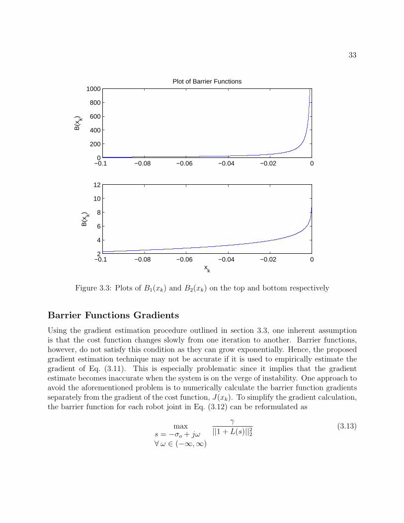
B(xk) is called a barrier function and is constructed such that these functions become arbi-trarily large if any one of the inequality constraints (i.e. R{cj,n} < 0) is about to violated.Common choices for B(xk) in Eq. (3.11) are:

B1(xk) = −∑j

∑n

ln{−ζj,nR{cj,n}}

B2(xk) = −∑j

∑n

−ζj,nR{cj,n}

(3.12)

where ζj,n serves as a scaling factor. Both function in Eq. (3.12) are plotted in Fig. 3.3.Note that both examples become arbitrarily large as R{cj,n} approach 0 from below. Afundamental assumption when using barrier methods is that the barrier functions are neverviolated when updating the free parameters xk. This criteria can be satisfied by properlychoosing the stepsize. Stepsize selection criteria will be discussed in a later subsection ofthis chapter.

On a technical note, in order for the solution of Eq. (3.11) to be exactly the same asthe original formulation in Eq. (3.10), one would have to iteratively solve Eq. (3.11) withthe coefficients ζj,n decreasing in each iteration. The optimal solution x∗

k(ζj,n) as each ζj,n isiteratively reduced to zero follows a trajectory known as the centralpath along the solutionspace. The limit point of these solutions is the solution to Eq. (3.10) [4]. For the purpose ofgain tuning, however, Eq. (3.11) is not solved iteratively, but instead is treating as its ownoptimization problem. Hence the optimal solution for the feedback controller gains usingthe barrier method may not be same as the one obtained by solving Eq. (3.10). This is nota problem in this application as long as the gain tuning algorithm can continue to improvethe robot performance. This can be guaranteed by initially setting each x∗

k(ζj,n) such thatJ(x1) ≫ B(x1) based on the initial values for x1. This way, any substantial decrease of thecombined cost function is caused by improved performance and not by the barrier functions.

33

−0.1 −0.08 −0.06 −0.04 −0.02 00

200

400

600

800

1000

B(x

k)Plot of Barrier Functions

−0.1 −0.08 −0.06 −0.04 −0.02 02

4

6

8

10

12

xk

B(x

k)

Figure 3.3: Plots of B1(xk) and B2(xk) on the top and bottom respectively

Barrier Functions Gradients

Using the gradient estimation procedure outlined in section 3.3, one inherent assumptionis that the cost function changes slowly from one iteration to another. Barrier functions,however, do not satisfy this condition as they can grow exponentially. Hence, the proposedgradient estimation technique may not be accurate if it is used to empirically estimate thegradient of Eq. (3.11). This is especially problematic since it implies that the gradientestimate becomes inaccurate when the system is on the verge of instability. One approach toavoid the aforementioned problem is to numerically calculate the barrier function gradientsseparately from the gradient of the cost function, J(xk). To simplify the gradient calculation,the barrier function for each robot joint in Eq. (3.12) can be reformulated as

maxs = −σo + jω∀ ω ∈ (−∞,∞)

γ

||1 + L(s)||22(3.13)

34

where L(s) is the open loop transfer function and σo is a positive tolerance term. Eq. (3.13)essentially performs a search along a vertical line in the complex plane whose real part isgiven by −σo. Eq. (3.13) will grow rapidly as the closed loop poles approach −σo. Like allbarrier methods, this approach assumes that initially all the real components of the closedloop poles are less than −σo and updating the controller gains do not cause the poles tocross −σo. The first assumption can be checked by properly selecting the initial controllergains. The second assumption can be satisfied through careful stepsize selection. The valueof s in Eq. (3.13) can be found through a numerical search using commercial software suchas MATLAB. Assuming s = σo + jωo is known, the gradient of the barrier function can becomputed . To simplify the algebra, consider the following notation

s = σo + ωojs2 = (σ2

o − ω2o) + (2ωoσo)j

= ϕ1 + ϕ2js3 = (σoϕ1 − ωoϕ2) + (ωoϕ1 + σoϕ2)j

Gdmu(s) = θm(s)u(s)

=Jls

2+djs+kjJmJls3+Jds2+Jks+kjdm

= β22s2+β1s+βo

α3s3+α2s2+α1s+αo

= (β2ϕ1+β1σo+βo)+(β2ϕ2+β1ωo)j(α3(σoϕ1−ωoϕ2)+α2ϕ1+α1σo+αo)+(α3(ωoϕ1+σoϕ2)+α2ϕ2+α1ωo)j

= γ1+γ2jδ1+δ2j

L(s) = γ1+γ2jδ1+δ2j

Kvs2+(KvKp+Ki)s+KpKi

s2

where j =√−1. The expressions above breaks the complex values into their corresponding

real and imaginary parts. This is convenient since it allows Eq. (3.13) to be expressed as

1||1+L(σo+jωo)||2 = 1

wTw (3.14)

where w = [ℜe{1 + L(σo + jωo)} ℑm{1 + L(σo + jωo)}]T . From (3.14), the gradient of thebarrier function can be expressed as

∂

∂xk

1

||1 + L(σo + jωo)||2=

∂w

∂xk

−2w

(wTw)2(3.15)

Since the current application of the gain tuning algorithm focuses on tuning the feedbackcontroller gains, the free variables for the NLP are the feedback controller parameters. More

35

specifically, xk = [Kp Kv Ki]T . To evaluate ∂w

∂xk∈ R3×2, consider the following notation

γ1+γ2j(δ1+δ2j)s2

= {ϕ1(γ1δ1+γ2δ2)+ϕ2(γ2δ1−γ1δ2)}+{ϕ1(γ2δ1−γ1δ2)−ϕ2(γ1δ1+γ2δ2)}j||δ1+δ2j||2 ||ϕ1+ϕ2j||2

= θ1+θ2j||δ1+δ2j||2 ||ϕ1+ϕ2j||2

L(σo + jωo) = θ1+θ2j||δ1+δ2j||2 ||ϕ1+ϕ2j||2{Kvs

2 + (KvKp +Ki)s+KpKi}

ℜe{1 + L(σo + jωo)} = 1 + θ1(Kvϕ1+(KvKp+Ki)σo+KpKi)−θ2(Kvϕ2+(KvKp+Ki)ωo)

||δ1+δ2j||2 ||ϕ1+ϕ2j||2

ℑm{1 + L(σo + jωo)} = θ2(Kvϕ1+(KvKp+Ki)σo+KpKi)+θ1(Kvϕ2+(KvKp+Ki)ωo)

||δ1+δ2j||2 ||ϕ1+ϕ2j||2

The first and second columns of ∂w∂xk

are ∂∂xk

ℜe{1+L(σo+jωo)} and ∂∂xk

ℑm{1+L(σo+jωo)}respectively. Evaluating these partial derivatives yield

∂∂xk

ℜe{1 + L(σo + jωo)} = 1||δ1+δ2j||2 ||ϕ1+ϕ2j||2

θ1(σoKv +Ki)− θ2ωoKv

θ1(ϕ1 + σoKp)− θ2(ϕ2 +Kpωo)θ1(σo +Kp)− θ2ωo

∂

∂xkℑm{1 + L(σo + jωo)} = 1

||δ1+δ2j||2 ||ϕ1+ϕ2j||2

θ2(σoKv +Ki) + θ1ωoKv

θ2(ϕ1 + σoKp) + θ1(ϕ2 +Kpωo)θ2(σo +Kp) + θ1ωo

Hence, ∂∂xk

1||1+L(σo+jωo)||2 = ∂w

∂xk

−2w(wTw)2

can be evaluated using the equations listed above.

3.5 Stepsize Selection

As mentioned earlier, the selection of the stepsize, αk, needs to ensure that updating thecontroller gains will not violate the barrier constraints. If the barrier functions are accuratelydefined, then enforcing the barrier functions will also guarantee system stability. Manytraditional stepsize selection techniques require knowledge of how the stepsize affects theupdated cost function, J(xk+1). Examples of these techniques include the Goldstein ruleand the Armijo rule. In this particular application, the cost function J(xk) does not havea closed form expression and can only be obtained through experimental measurements.Hence it is not possible to utilize many of these existing stepsize selection techniques. Whilethe cost function itself cannot be computed without performing an experiment on the robot,the barrier functions can be. Hence a successive stepsize reduction algorithm is used tocontinually reduce the stepsize until the updated gains satisfy the barrier functions.

36

In general, the stepsize, αk, can be represented more generally as

αk = α0,kαnkr (3.16)

where α0,k is the initial stepsize at iteration k, αr < 1 is a stepsize reduction ratio, andnk is the stepsize reduction factor at iteration k. Intuitively, if the initial stepsize violatesthe barrier constraints at a particular iteration, nk can be increased to decrease the stepsize.For the purpose of automatic gain tuning, it is important that the stepsize is selected toboth improve system performance while simultaneously enforcing system stability. In thisdissertation the selection of α0,k is used to improve performance while the selection of nk isused to satisfy the second requirement. Given that the gains are being updated using steepestdescent, a first order approximation shows that any positive value for α0,k is guaranteed todecrease the cost function. The caveat to this statement, however, is that it is only true forα0,k small enough such that the first order effects are dominant. Since ”small” also dependsheavily on the nonlinearity of the cost function, it is usually very difficult to quantify agood value for α0,k if the cost function is unknown. This dissertation uses a fixed value forα0,k for every iteration. The selected value is manually tuned based on experimental data.Additional refinement of α0,k is a topic of future work. Calculating nk, however, is relativelystraight forward since the barrier functions can be numerically evaluated prior to running theexperiment. Hence one can check whether or not updating the gains will violate the barrierconstraints. In this dissertation, nk is selected using the logic tree presented in Fig. 3.4.

3.6 Initial Condition Selection

Due to the nonlinear nature of the robot system, and inherently of the cost function J(xk),NLP techniques can only arrive at locally optimal solutions rather than globally optimalsolutions. Hence selecting the appropriate initial feedback controller gains prior to tuning canstrongly affect the performance of the gain tuning algorithm. In particular for an industrialrobot, tuning the three wrist joints (J4-J6) is particularly difficult as these joints tend to bevery sensitive to controller parameter variations. Hence it is especially important to correctlyselect the initial gains for these values. This subsection will provide a theoretical way forselecting initial gains to satisfy certain performance criterion. For practicality, the work inthis subsection will focus on selecting gains for the three wrist joints of the FANUC M-16iBrobot. Two gain selection approaches will be given. The first is a standard approach thatis commonly used in industry, whereas the second is a slightly more complicated approachwhich gives consideration to system stability and unmodeled dynamics.

Standard Initial Gain Selection Method

The feedback controller structure for a single wrist joint of the FANUC M-16iB is depictedin Fig. 3.5. Note that Fig. 3.5 uses motor velocity, θm, for motor side feedback. Note that

37

��

nk = 0

αk = αo,kαnkr

xk+1 = xk − αk∇J(xk)

��

�� xk+1

��

��

nk = nk + 1

��

��

��

��

Figure 3.4: Logic tree for selecting nk

since the load side inertias of the wrist joints are relatively small, the reducer dynamicsfor these three joints can be effectively ignored. Using this assumption, the wrist joint canbe approximated as an inertia system with viscous damping. This allows Eq. (2.7) to besimplified as a first order system of form:

Gdmu(s) =θm(s)

u(s)≈ Gdmu(s) =

1

Js+D(3.17)

where the lumped inertia and damping are given by J = Jm + JlN2 and D = dm respectively.

38

ufbKp−

∫

+

−

+ Kv

Ki

+��

� ��θmθm,ref

uff + uref

+

e

G(s)

θl

∫

��

+

r

Figure 3.5: Feedback controller structure for an individual joint

Additionally, also note that the controller structure can be broken down into two sepa-rate loops: an inner velocity loop and an outer position loop. This structure can simplifythe tuning process as the bandwidth of the inner and outer loop can be tuned separately.Performing a closed loop analysis of the inner loop from r to θm gives the following transferfunction:

θmr

=Kvs+Ki

Js2 + (Kv +D) s+Ki

(3.18)

Based on this observation, it would be ideal if the inner loop behaved like a first order closedloop system of form:

θmr

=1

δs+ 1(3.19)

This can be achieved by setting Kv = J/δ and Ki = D/δ. Once this is done, tuning of theouter loop is performed while assuming that the inner loop behaves like Eq. (3.19). Theproportional gain, Kp, is tuned such that the outer loop has the desired bandwidth. Notethat this method works if the outer loop bandwidth is significantly less than that of theinner loop bandwidth. While this method is simple to apply, it does not give considerationto any unmodeled system dynamics. Furthermore, there is no guarantee that these initialgains can even stabilize the system.

Alternate Initial Gain Selection Method

The bandwidth of a control loop is often used in practice as a measure of performance. Thealternate method for initial gain selection also aims at satisfying bandwidth requirements, butalso give considerations to stability and unmodeled dynamics. In the aforementioned tuningmethod, the inner loop and outer loop are tuned separately. When tuning the inner loop,however, it is inherently assumed that the plant behaves strictly like a first order dampedinertia system. More specifically, this process assumes the plant to behave like this ideal firstorder system up to the bandwidth specified by the time constant δ, which can in practice be

39

100

101

−20

0

20


dB

100

101

−200

−100

0

100

Deg

Hz (1/s)

Figure 3.6: System identification result for joint 4 (Blue circles indicate the measured fre-quency response from a sine sweep, black crosses indicates the response of an ideal first ordermodel)

as high as 20 Hz. In actuality, however, this assumption may not hold, and depending onthe actual dynamics of the plant, setting the values of Kv and Ki carelessly can cause theinner velocity loop to be unstable. Rather than making assumptions about the behavior ofthe plant, another approach is to use the system identification data to better characterizethe actual dynamics of the plant. The frequency response of J4-J6 are shown in Figs. 3.6-3.8. The blue circles indicate the measured system response from a sine sweep identificationexperiment whereas the black crosses indicate the frequency response of an ideal first orderdamped inertia model given by Eq. (3.17). The inertia parameters, Jm and Jl, used for thecalculations of the damped inertia model was provided by FANUC Corporation. The motorside viscous damping parameter, dm, was experimentally verified by Chen in [8]. Note thatFigs. 3.6-3.8 suggest that the first order approximation is accurate at low frequencies, butfails to capture the behavior of the system at higher frequencies. Notably, the first ordermodel is accurate up to about 10 Hz.

When tuning the bandwidth of the two feedback loops in Fig. 3.5, one thing to note isthat the only bandwidth that ultimately matters for actual performance is the outer loopbandwidth. As a result, the inner loop bandwidth does not necessarily matter as long as theouter loop maintains its desired bandwidth.

40

100

101

0

20

40


dB

100

101

−200

−100

0

100

Deg

Hz (1/s)


Inner Loop Bandwidth Analysis

In the standard approach, the inner loop is tuned to behave like the first order system givenby Eq. (3.19). Eq. (3.18) shows that the inner loop is naturally second order. While forcingit to behave like a first order makes it simple for tuning the outer loop, this approach maynot be very robust to modeling uncertainties. A more straightforward and robust approachis to directly analyze the bandwidth of the second order system. This section will detailthe bandwidth analysis for a second order system in the form given by Eq. (3.18). Thebandwidth of Eq. (3.18) is defined as the lowest frequency, ω in which:∣∣∣∣∣ θmr

∣∣∣∣∣s=jω

=

∣∣∣∣∣ Ki

J

s2 + (Kv+D)J

s+ Ki

J

· Kvs+Ki

Ki

∣∣∣∣∣s=jω

<1√2

(3.20)

Rewriting the second order term in Eq. (3.20) as ω2n

s2+2ζωns+ω2nand then squaring both sides

of Eq. (3.20) yields:ω4n

K2i

· K2vω

2 +K2i

(ω2n − ω2)2 + (2ζωnω)2

<1

2(3.21)

41

100

101

20

30

40


dB

100

101

−100

−50

0

50

Deg

Hz (1/s)


where ζ = (Kv+D)

2√KiJ

and ω2n = Ki/J . After some algebraic manipulation and also setting the

inequality to an equality, the solution to ω in Eq. (3.21) can be written as:

ω2 = K2v+JKi−2JKiζ

2

J2

± [4ζ4K2i J

2−4ζ2K2i J

2−4ζ2K2vKiJ+2JK2

vKi+K4v+2J2K2

i ]1/2

J2

(3.22)

Solving Eq. (3.22) for the smallest positive value of ω will yield the bandwidth of the innerloop for given controller gains Ki and Kv. Upon careful observation of Eq. (3.22) one canshow that the term under the square root is larger than the leading term, hence the solutionof interest can be expressed as:

ω2 = K2v+JKi−2JKiζ

2

J2

+[4ζ4K2

i J2−4ζ2K2

i J2−4ζ2K2

vKiJ+2JK2vKi+K4

v+2J2K2i ]

1/2

J2

(3.23)

To prevent overshoot in the system response, it is desirable to set the value ζ = 1. By doingso, Ki becomes a function of Kv through the following relationship:

Ki =(Kv +D)2

4J(3.24)

42

Substituting this relationship into Eq. (3.23) yields the following expression:

116K4

v +D4K3

v +(

3D2

8+ 3J2ω2

2

)K2

v +(

D3

4−DJ2ω2

)Kv+(

D4

16− J4ω4 − J2ω2D2

2

)= 0

(3.25)

Once the desired bandwidth, ω, is fixed by the designer, a numeric solver can be used tosolve Eq. (3.25) for Kv. Once Kv is known, Eq. (3.24) can be used to solve for Ki.

Outer Loop Bandwidth Analysis

Once the inner loop is tuned, as long as the bandwidth of the inner loop is substantiallyhigher than the desired bandwidth of the outer loop, the the inner loop can be treated asan unit gain when doing the outer loop analysis. At low frequencies, the outer loop transferfunction effectively becomes:

θm

θmd

=Kp

s+Kp

(3.26)

Hence Kp can be designed to shape the outer loop bandwidth.

Final Initial Controller Gain Adjustments

Once the initial controller gains are calculated using the analysis approach outlined in theprevious two sections, the final step is to lower Kv as much as possible while still maintainingthe desired outer loop bandwidth. Recall that decreasing Kv will decrease the inner loopbandwidth but it may not affect the outer loop bandwidth. This final step is to ensure thatthe initial gains do not cause the mechanical system to become unstable.

3.7 Experimental Results

In this section, the M-16iB is used to verify the proposed gain tuning algorithm. In thisdissertation, a quadratic cost function that penalizes the tracking position error and velocityerror is used. Since the built in robot motor encoders can readily provide motor position andvelocity error information, the motor side error is used when computing the cost function.Using the motor side error is sufficient for demonstrating the feasibility of the proposedapproach, but in practice, the cost function should penalize the load side errors. Morespecifically, the cost function used in the dissertation has form:

J(xk) =T∑t=0

{eTm,k(xk, t)W1(t)em,k(xk, t) + eTm,k(xk, t)W2(t)em,k(xk, t)} (3.27)

43

where t is a time index, em,k(t) and em,k(t) is the motor side position error and velocityerror vector respectively. W1(t) and W2(t) are the weighting matrices for the motor sideposition and velocity errors respectively. Additionally, the barrier function parameters σo

and γ were manually tuned for each joint so that the initial contributions from the barrierfunctions to the entire cost function were an order of magnitude less than the contributionsfrom the tracking errors em(t) and em(t). The initial stepsize, αo,k, and step size reductionratio, αr, were both selected to be 0.5. The perturbation amplitudes for each controller gainwas selected to be 10% of their initial value. And finally, 65 iterations were used for the gaintuning process.

Single Joint Tuning Experiments

This section presents the results from the single joint tuning experiments on the M-16iBrobot. The perturbation frequencies used forKp, Kv, andKi were 0.293π, 0.467π, and 0.313πrespectively for each joint. Since each joint is tuned individually, the weighting matrices W1

and W2 reduce to scalars. Values of 1 and 0.3 were used for W1 and W2 respectively. Inthese tuning experiments, each joint of the robot was instructed to sweep a 22.5 degree arcover one second and then sweep back. The initial and final controller gains for each joint istabulated in Table 3.1.

Figures. 3.9-3.14 plot the cost function versus iteration for each joint. Note that in somecases, it requires up to 30 iterations before the cost function begins to substantially decrease.This can be caused by many factors, such as the initial gains starting off in a local plateauin the map between the cost function and controller gains. Since the gains are perturbedfrom iteration to iteration, the effects of these perturbations can been in the cost function.Since the sensitivity of the cost function to these perturbations vary from one set of gains toanother, it may cause the cost function to decrease nonmonotonicly. Also note that for J1,J2, J3 and J5, the contributions of the barrier functions to the overall cost function seemminimal. This is to be expected if the tuning process does not encounter any gains that maydestabilize the system. For some joints, in particular J4 and J6, the contributions from thebarrier functions are not negligible. Both J4 and J6 were found to be extremely sensitive totheir velocity gain Kv. While increasing Kv improves performance, increasing it beyond acertain value would abruptly cause the joint to chatter significantly. As a result, the barrierfunction parameter γ was set to be more conservative for these two joints to preserve overallsystem stability. This effect can be seen in Fig. 3.14 after 30 iterations and to a lesser extentin Fig. 3.12. Even with these nuances, however, the gain tuning method still decreased theperformance-based portion of the cost function (dashed lines), thus resulting in improvedtracking performance of the robot manipulator.

44

Table 3.1: Parameters for gain tuning

ParametersJoint Kp,1 Kv,1 Ki,1 Kp,65 Kv,65 Ki,65

J1 10 0.2300 0.1000 10.293 0.3493 0.1257J2 10 0.2000 0.1000 10.030 0.2250 0.1310J3 10 0.0507 0.0100 9.991 0.1010 0.0954J4 20 0.0560 0.2000 19.998 0.0622 0.2010J5 15 0.0020 0.0020 15.000 0.0025 0.0024J6 20 0.0040 0.0040 19.999 0.0069 0.0035

3.8 Chapter Summary

This chapter introduced an automatic gain tuning algorithm using nonlinear programming.The proposed gain tuning procedure was presented and barrier functions were introducedto help preserve system stability during tuning. Additionally, this chapter also introducedtechniques for selecting the stepsize and initial gains when utilizing this tuning algorithmon industrial robots. And finally, experimental results were presented to verify the utility ofthe proposed approach.

45

0 10 20 30 40 50 60 700.015

0.02

0.025

0.03

0.035

0.04

0.045Cost Function for Tuning J1

Iterations

Cost FunctionCost Function (w/out Barrier)

Figure 3.9: Cost function versus iteration while tuning J1 of the FANUC M-16iB robot

46

0 10 20 30 40 50 60 704.5

5

5.5

6

6.5

7

7.5x 10

−3 Cost Function for Tuning J2

Iterations



47

0 10 20 30 40 50 60 700.005

0.01

0.015

0.02

0.025


Iterations



48

0 10 20 30 40 50 60 70

0.16

0.18

0.2

0.22

0.24


Iterations



49

0 10 20 30 40 50 60 702

2.5

3

3.5

4

4.5

5Cost Function for Tuning J5

Iterations



50

0 10 20 30 40 50 60 700

0.1

0.2

0.3

0.4

0.5

0.6

0.7


Iterations



51

Chapter 4

A Disturbance Observer Frameworkfor Stable Feedback Controller Tuning

4.1 Introduction

This chapter introduces a disturbance observer based framework for stable feedback con-troller tuning. When tuning high order controllers with a plant whose behavior is not fullyknown, feedback controller tuning always run the risk of destabilizing the system. Barring afew mild restrictions, this chapter presents a tuning framework that allows one to arbitrarilytune a subset of the feedback controller parameters while simultaneously preserving systemstability. This chapter begins by briefly reviewing the traditional disturbance observer insection 4.2 before introducing the framework in section 4.3. The motivation and proof for theframework is also presented. Both simulation and experimental verification of the frameworkare organized in section 4.4. Finally, the contents of the chapter is summarized in section 4.5.

4.2 Traditional Disturbance Observer

The structure of a typical disturbance observer (DOB) is show in Fig. 4.1. In the figure, Ga(s)is the phyiscal plant, G−1

n (s) is the stable nominal inverse of the plant, and Q(s) is calledthe Q-filter and is to be designed. U∗(s), D(s), Y (s), and N(s) are the command input,disturbance input, plant output, and the measurement noise respectively. The disturbanceobserver has several beneficial properties, namely the transfer function U∗(s) to Y (s) is givenby:

Gyu∗(s) =Ga(s)Gn(s)

Gn(s) +Q(s) (Ga(s)−Gn(s))(4.1)

If Q(s) = 1, then Gyu∗(s) = Gn(s). Similarly, if Q(s) = 0, then Gyu∗(s) = Ga(s). Thisimplies that the DOB structure will force the input/output relationship from U∗(s) to Y (s)to behave like the nominal model within the pass band of the Q-filter, and to behave like

52

+

−

U∗(s)

+

U(s)

D(s)

Ga(s)

+

Y (s)

N(s)G−1

n(s)+

−

Q(s)

Figure 4.1: Typical DOB structure

Ga(s) in the stop band of the Q-filter. Additionally, the DOB structure has modest stabilityrobustness properties, especially if Gn(s) closely matches Ga(s) within the pass band of theQ-filter. Traditionally, the Q-filter is designed as a lowpass filter whose bandwidth is limitedby the error between Gn(s) and Ga(s).

4.3 Disturbance Observer Tuning Framework

In most controller applications applications, the controllers are tuned to provide good systemperformance up to a predesignated bandwidth. While increasing the controller gains willimprove the system performance within the desired bandwidth, recklessly increasing thegains may also cause the controller to excite resonances and other high frequency dynamicsof the physical system. This in effect will deteriorate the overall system performance andin the worst case destabilize the system. Many established controller tuning methods suchas the Ziegler-Nichols method operate by effectively giving practical guidelines for balancingthe trade off between good low frequency performance and overall system stability.

So if the desired system bandwidth is known in advance, it would be ideal if tuning thefeedback controller would just affect the closed loop system performance within this desiredclosed-loop bandwidth. A naive implementation of this idea can be done with the parallelcontroller structure shown in Fig. 4.2. C(s) is a fixed stabilizing controller for plant G(s).Ct(s) is the controller being tuned and Q(s) is a lowpass filter whose cutoff frequency dictatesthe desired bandwidth of the tuned controller. R(s), E(s), U(s), and Y (s) are the referencesignal, error, plant input, and plant output respectively. The equivalent controller in Fig. 4.2can be expressed as:

Ceq(s) =(1− Q(s)

)C(s) + Q(s)Ct(s) (4.2)

53

Ceq(s)

E(s)

+

−

R(s)E(s)

C(s) +

Y (s)U(s)

Ct(s)Q(s)

1− Q(s) G(s)

Figure 4.2: Parallel controller structure

Roughly speaking, Ceq(s) behaves like Ct(s) in the passband of Q(s) and behaves like C(s)otherwise. This implementation has several key advantages when it comes to gain tuning.Normally, engineers can use a nominal model, G(s), to model the physical plant G(s). Dueto both computational and modeling limitations, these nominal models capture the behaviorof G(s) well at low frequencies, but are unable to capture the higher frequency dynamics.Additionally, most physical plants tend to exhibit nonlinear amplitude dependent behaviorat higher frequencies. For these reasons, typical feedback controller gains are limited. Byusing a framework similar to that shown in Fig. 4.2, the controller gains in Ct(s) can betuned without experiencing the aforementioned limitations. While it is easy to draw intuitivestatements about the performance of the structure in Fig. 4.2, rigorously proving the internalsystem stability for such a structure, however, turns out to be very difficult.

Motivation

Recalling the input/output relationship of the DOB in Eq. (4.1), one may note that thistransfer function has similar characteristics as Eq. (4.2). Namely, both structures allow thecombined transfer function to behave like one transfer function within a certain bandwidthand behave like another independent transfer function outside of that bandwidth. Mostimportantly, these two transfer functions are completely separated in the block diagram,hence one can be adjusted without affecting the other. Using Figs. 4.1-4.2 as inspiration,the DOB tuning framework is shown in Fig. 4.3.

Like before, C(s) is a fixed and stabilizing controller for the plant G(s). C−1t (s) is the

inverse of the controller being tuned and Q(s) is the Q-filter that is to be designed by theuser. Using this framework, the relationship from the error E∗(s) to U(s) is given by:

Cue∗(s) =C(s)Ct(s)

Ct(s) +Q(s) (C(s)− Ct(s))(4.3)

Similar to the behavior in Eq. (4.1), Cue∗(s) behaves like Ct(s) when Q(s) = 1 and like C(s)when Q(s) = 0. This is important, since it allows Ct(s) to only affect particular frequency

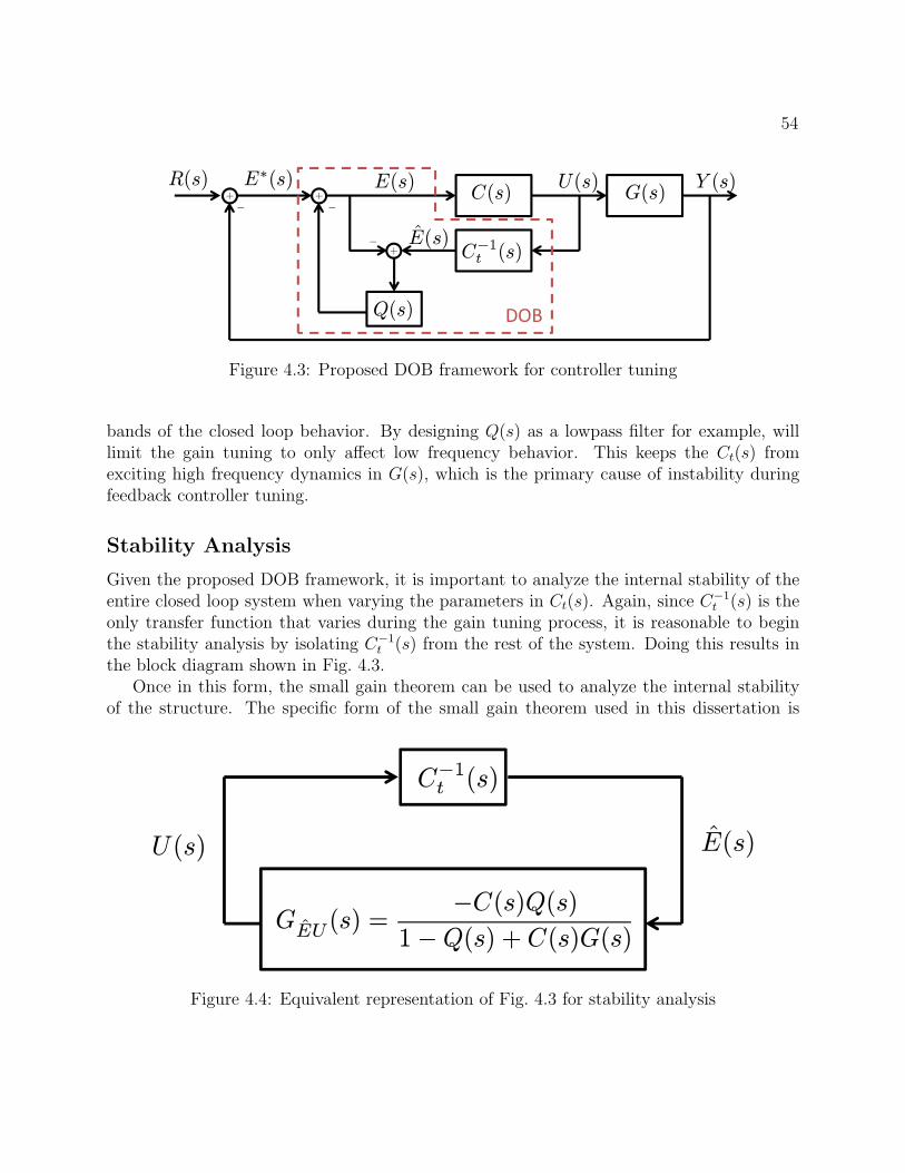
54

Y (s)E(s)

E(s)

+

−

U(s)C(s)

R(s)

C−1

t(s)+

−

Q(s)

+ G(s)−

��

E∗(s)

Figure 4.3: Proposed DOB framework for controller tuning

bands of the closed loop behavior. By designing Q(s) as a lowpass filter for example, willlimit the gain tuning to only affect low frequency behavior. This keeps the Ct(s) fromexciting high frequency dynamics in G(s), which is the primary cause of instability duringfeedback controller tuning.

Stability Analysis

Given the proposed DOB framework, it is important to analyze the internal stability of theentire closed loop system when varying the parameters in Ct(s). Again, since C−1

t (s) is theonly transfer function that varies during the gain tuning process, it is reasonable to beginthe stability analysis by isolating C−1

t (s) from the rest of the system. Doing this results inthe block diagram shown in Fig. 4.3.

Once in this form, the small gain theorem can be used to analyze the internal stabilityof the structure. The specific form of the small gain theorem used in this dissertation is

E(s)U(s)

C−1

t(s)

GEU

(s) =−C(s)Q(s)

1−Q(s) + C(s)G(s)

Figure 4.4: Equivalent representation of Fig. 4.3 for stability analysis

55

+

−Q(s)

G(s)C(s)

C(s)

−1

G(s)

Figure 4.5: Block diagram representation of GEU as a structured uncertainty problem

formally stated as follows:

Theorem 1. If two systems S1(s) and S2(s) are connected in a positive feedback loop, thenthe closed loop system is internally stable if both S1(s) and S2(s) are internally stable and if∥S1(s)S2(s)∥∞ < 1.

Remark The general small gain theorem was derived by Zames and the proof will not berepeated here [41]. The specific form of the small gain theorem used in this dissertation isthe form commonly used to analyze stability of systems with bounded uncertainty and oftenused in conjunction with H∞ controller synthesis.

Based on the small gain theorem, the first two conditions to check are the internal stabilityconditions of C−1

t (s) and GEU(s). Since C−1t (s) is a controller that is actively being tuned,

its stability can be easily enforced while tuning. The internal stability of GEU(s) on theother hand, is harder to analyze. Rather than directly analyzing the stability of GEU(s), it

is more convenient to look at the stability of GEU(s), which is defined as:

GEU(s) =C(s)G(s)−Q(s)

1 + C(s)G(s)−Q(s)(4.4)

Note that GEU(s) and GEU(s) both have the same characteristic equation, hence showing

that GEU(s) is internally stable is the same as showing that GEU(s) is internally stable. It

is convenient to consider GEU(s) because it can be interpreted as a closed loop system withcontroller C(s) and plant G(s) where the plant has a structured multiplicative uncertainty

given by−Q(s)

G(s)C(s). This feedback system is depicted in Fig. 4.5. The following theorem is

helpful for interpreting the stability conditions of such a system:

56

Theorem 2. Given a plant with multiplicative structured uncertainty defined as Gunc(s) =G(s) (1 +Wu(s)∆(s)) where G(s) is the nominal plant representation as a rational transferfunction, Wu(s) is the structured uncertainty modeled as a stable transfer function, and ∆(s)is any transfer function such that ∥∆(s)∥∞ ≤ 1. Furthermore, it is assumed that thenumber of unstable roots of Gunc(s) remains the same and is equivalent to the number ofunstable roots of G(s) under all possible parameter variations characterized by the structureduncertainty model. If these conditions hold, then a controller C(s) stabilizes all variationsof Gunc(s) under negative feedback if and only:

1. C(s) stabilizes G(s)

2.

∣∣∣∣∣∣∣∣Wu(s)G(s)C(s)

1 +G(s)C(s)

∣∣∣∣∣∣∣∣∞

< 1

Proof. The proof for Theorem 2 can be constructed graphically. The dashed line in Fig. 4.6is the Nyquist plot of the open loop transfer function G(s)C(s). The structured uncertaintyof Gunc(s) implies that at any point s = jω along the Nyquist plot, Gunc(jω)C(jω) cantake any value within a spherical region centered around G(jω)C(jω) with radius r(ω) =∥Wu(s)G(s)C(s)∥s=jω. The first condition implies that the Nyquist plot of G(s)C(s) hasthe correct number of encirclements of −1 to guarantee closed loop system stability. Sinceit is assumed that the number of unstable roots of Gunc(s) is the same as the number ofunstable roots of G(s), the Nyquist criteria states that Gunc(s)C(s) will also be closed loopstable under all possible outcomes of the proposed structural uncertainty if none of theseuncertainties can change the number of encirclements of Gunc(s)C(s) about −1. Anotherway to write this condition is for the radius of uncertainty, r(ω) = ∥Wu(s)G(s)C(s)∥s=jω, tobe less than ∥1+G(jω)C(jω)∥ for all frequencies. This is exactly the second condition of thetheorem. Additional discussion regarding the derivation and implications of this theoremcan be found in [37].

It is relatively straight forward to apply Theorem 2 to show the stability of GEU(s). Onepossible application of the theorem is to set:

Wu(s) = −Q(s)G(s)C(s)

∆(s) = 1

One can quickly confirm that the assumptions in Theorem 2 can be easily satisfied for thesystem at hand. Going through the checklist:

1) G(s) needs to be represented as a rational transfer function: this requirement canbe satisfied through preliminary models of the system.

2) Wu(s) must be a stable transfer function: since in this particular application,

Wu(s) = −Q(s)G(s)C(s)

, stability can be guaranteed if G(s) and C(s) are minimum phase

57

G(jω)C(jω)G(jω)C(jω)

r(ω)

r(ω) = ||Wu(jω)G(jω)C(jω)||

−1

Figure 4.6: Nyquist plot of C(s)G(s)

and if Q(s) is stable. These requirements are generally not problematic as most indus-trial robots are minimum phase systems. Furthermore non-minimum phase controllersand unstable filters are usually avoided in feedback loops, hence this requirement canbe easily satisfied.

3) The number of unstable roots of GEU(s) must be the same as those in G(s). Thisconstraint can be violated in two ways:

i. Introduction of an unstable pole by the uncertainty term.

ii. Elimination of an unstable pole by the uncertainty term.

Since GEU(s) can also be rewritten as:

GEU(s) = G(s)

(1− Q(s)

G(s)C(s)

)(4.5)

58

An additional unstable pole can be inserted only if Q(s)G(s)C(s)

is unstable, which violatesthe previous constraint. An existing unstable pole can be removed if a unstable pole

zero cancellation occurs between the G(s) and(1− Q(s)

G(s)C(s)

). Again, since C(s) and

Q(s) are designed by the user, this scenario can be easily avoided.

Now to apply Theorem 2. The first condition states that GEU(s) is stable if and only ifC(s) is a stabilizing controller for G(s), which is trivially satisfied. More interestingly, thesecond condition states that: ∣∣∣∣∣∣∣∣ −Q(s)

1 +G(s)C(s)

∣∣∣∣∣∣∣∣∞

< 1 (4.6)

Eq. 4.6 suggests that magnitude the product of Q(s) and the sensitivity function of thenominal closed loop plant with controller C(s) must be upper bounded by 1. This naturallyleads to Q(s) to be designed as a low pass filter. And GEU satisfies the theorem, which showsthat the transfer function is stable, and that consequently also shows that GEU is stable. Atthis point, the small gain theorem says that the DOB framework (Fig. 4.4) is stable if:∣∣∣∣∣∣∣∣ −C−1

t (s)C(s)Q(s)

1−Q(s) + C(s)G(s)

∣∣∣∣∣∣∣∣∞

< 1 (4.7)

Eq. (4.7) is only interesting within the pass band of Q(s). Setting Q(s) = 1 suggests that:∣∣∣∣∣∣∣∣ −1

Ct(s)G(s)

∣∣∣∣∣∣∣∣∞

< 1 (4.8)

Eq. (4.8) suggests that there is a lower bound on the controller gains for Ct(s) but notnecessarily an upper bound. This condition is useful for gain tuning applications sincein most gain tuning scenarios, the gains are increases for better performance rather thandecreased.

Limitations

There are a few limitations with the DOB framework, many of these are mild limitationsand should not affect the overall effectiveness of such a framework. A summary of theselimitations are as follows:

1) C−1t (s) is required to be stable: This condition is introduced so that the small gain

theorem can be applied to the system shown in Fig. 4.4. This condition implies thatthe tuned block Ct(s) should not introduce unstable zeros to the equivalent controllergiven by Eq. 4.3. This constrain is reasonable since Bode’s Integral Theorem suggeststhat right half plane zeros can put limitations on the system’s performance.

59

2) G(s) and C(s) cannot contain any unstable zeros: This constraint is notably prob-lematic if the physical plant has non-minimum phase characteristics. Although forindustrial robot applications, most robots are indeed minimum phase, hence the plantconstraint should not be an issue. Additionally, since C(s) is designed to be any stabi-lizing controller for G(s), it should not be difficult to introduce a stabilizing controllerwith minimum phase properties.

3) Q(s) needs to be stable and designed in a way such that Eq. (4.6) is satisfied:The stability condition of Q(s) is implied by the structure of the DOB framework toensure internal stability. As previously mentioned, Eq. (4.6) suggests that Q(s) can benaturally designed as a lowpass filter. This coincides well with the initial motivationfor the DOB structure. The only limitation set by Eq. (4.6) is that the bandwidth ofQ(s) is limited by the closed loop performance of the stabilizing controller C(s).

As a result, while a few constraints are introduced to enforce system stability, closer analysisshow that these constraints do not hinder the practical application of the DOB framework.

4.4 Results

This section attempts to verify the stability properties of the proposed DOB frameworkthrough both simulations and experiments. The nominal plant model used for each joint ofthe FANUC M16iB robot is a fifth order transfer function that is designed to closely matchthe robot system identification data up until 20 Hz. Both C(s) and Ct(s) are chosen to bePID controllers with form:

C(s) =Kvs

2 + (KvKp +Ki) s+KpKi

s2(4.9)

Ct(s) =Kvts

2 + (KvtKpt +Kit) s+KptKit

s2(4.10)

The gains of C(s) are conservatively selected such that C(s) is a minimum phase controllerthat can stabilize the robot. C(s) and Ct(s) are chosen to be PID controllers so that theDOB framework can be directly compared with the M16iB’s existing PID structure. Q(s)is designed to be a lowpass filter with a 20 Hz bandwidth of form:

Q(s) =ω2n

s2 + 2ωns+ ω2n

(4.11)

where ωn = 40π. The selection of Q(s) and C(s) satisfy the conditions introduced in theprevious section to ensure stability of the DOB framework.

While it is difficult to prove that a particular system is stable for an unbounded set ofcontroller gains, the following table attempts to show that the system is stable for a wide

60

Kpt Kvt Kit

Gains in DOB Framework 0.06− 305 0.03− 1.02 0.00− 10.4Stable Gains in Default PID Structure 10− 20 < 0.25 < 1

Table 4.1: Verified stable gain variations in DOB framework through simulation

range of gains. In particular, the following data is collected from the fourth joint of theFANUC M16iB robot. Table 4.1 details the gain variations for Ct(s) which is still able tostabilize the system. Note that typical values for the PID gains using the default controllerstructure are given in the second row. The DOB framework is able to stabilize the systemfor a much higher range of gain variations. Table 4.2 provides a range of gains that are

Kpt Kvt Kit

Gains in DOB Framework 16.8− 168 0.035− 0.35 0.29− 2.9Stable Gains in Default PID Structure 10− 30 < 0.1 < 1

Table 4.2: Verified stable gain variations in DOB framework through experimentation

able stable through the DOB structure for the M16iB robot. These gains are verified andobtained through experimentation. Again, the typical values that can be used to stabilizethe standard PID controller are given in the second row. Note the much wider range ofstabilizing controller parameters.

With this said, there are several limitations with the DOB framework. Looking at Fig. 4.3,the entire feedback controller can be thought as a higher order controller whose order is upperbounded by the sum of the orders of C(s), Ct(s), and Q(s). While it’s straightforward todesign C(s) and Q(s) and subsequently tune Ct(s) to obtain the entire feedback controller,it is difficult to guarantee in advance the structure of the tuned controller. Hence theDOB framework may not be applicable if the hardware/software configuration does notallow for flexible feedback controller structures. A consequence of this limitation is thatthe framework cannot be applied to tune typical PID controllers found in many of today’smechanical systems.

4.5 Chapter Summary

This chapter presented a framework based on the disturbance observer for stable feedbackcontroller tuning. Both simulation and experimental results are provided to demonstrate therobust stability conditions of the DOB framework. A current limitations of this approach,however, is that it cannot be used to PID controllers. While the user can specify thecontroller being tuned to be of any structure, the complete controller is given by Eq. (4.3).The framework essentially allows the user to tune a subset of the parameters of a higher

61

order controller. While this increases the computational complexity of the entire controller,in return, it is able to provide very robust stability properties for the controller. At thispoint of development, the DOB framework cannot be utilized for tuning PID controllers butit may play a significant role in tuning higher order controllers in the future.

62

Chapter 5

An Input Shaping Method toSuppress Transient Vibrations InFlexible Joint Robotic Manipulators

5.1 Introduction

This chapter proposes an input shaping approach for suppressing the fundamental vibratorymode in flexible joint robots. In many robot manipulator applications, such as spot welding,it is desirable for the robot to travel quickly from one point to another. In these situations,the robot user is primarily concerned with suppressing the robot end effector vibrations asit approaches each point. As a result, it is important to develop methods that can suppresstransient vibrations. Section 5.2 briefly introduces the input shaping concept. Developmentof the proposed algorithm takes place in section 5.3. More specifically, section 5.3 discussesabout both the system identification aspect as well as the actual input shaping procedure.Both simulation and experimental results are given in section 5.4. Finally, section 5.5 sum-marizes the contents of this chapter.

5.2 Input Shaping

Input shaping was first proposed by the authors in [36]. As the name suggests, the methodinvolves modifying the desired system’s input such that the actual output from the closedloop system matches the initial desired trajectory. The initial theory assumes that the sys-tem contains damped vibratory modes that can be accurately modeled by linear vibrationanalysis. Using this assumption, impulses can be injected into the system at a π/2 phaseoffset to effectively cancel out the vibratory response of the system. While the fundamentaltheory lies heavily on linear vibration analysis, the effectiveness of the input shaping ap-proach was validated through experimentation on a more complex mechanism. Following

63

u θm

Jm

dm

fnl,m

dj

kj

N , θ, fnl,j

Jl

θl

��

��

Figure 5.1: Two inertial model of an indirect drive mechanism

this example, this chapter develops the underlying theory for the input shaping approachbased on linear vibration theory. But ultimately, the utility of the approach is demonstratedby both simulation and experimentation on the M-16iB industrial robot.

5.3 Theory

An individual joint of a robot manipulator can be approximated a two inertia model. Forreading convenience, the two inertia model originally presented in Fig. 2.1 is shown againhere in Fig. 5.1. In industrial robotic joints, both linear and non-linear joint dynamics exist.The linear portion is modeled in the two inertia model by the linear spring and damper whichhave constants kj and dj respectively. The nonlinear portion is modeled by the transmissionerror, θ, and the generic variable fnl,j. Unfortunately in most systems, nonlinear dynamicsis difficult to model and predict. Unless more information about these nonlinear effects isknown, it is not possible to compensate for them without the use of load side sensors. Sincethis nonlinear behavior is difficult to learn and generalize for any given input, the focus of theinput shaping technique presented in this chapter will focus on learning and compensatingfor the linear component of the transmission dynamics, namely the fundamental vibratorymode.

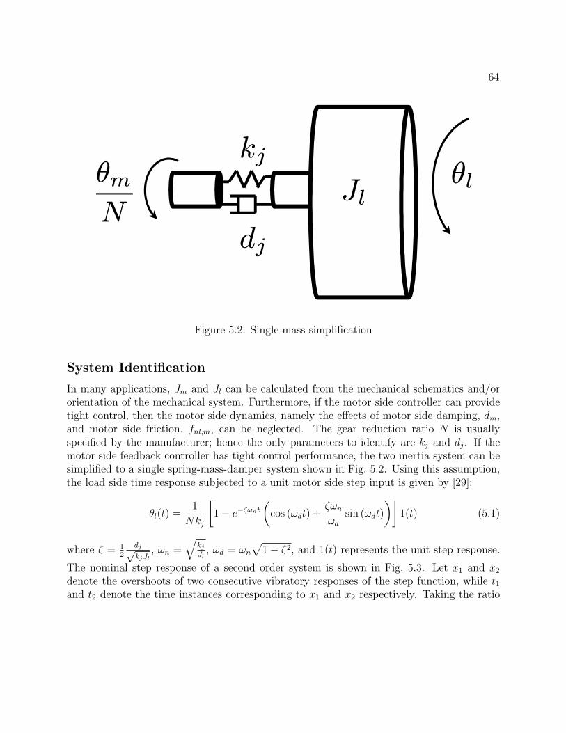
64

θm

N

dj

kjθl

Jl

Figure 5.2: Single mass simplification

System Identification

In many applications, Jm and Jl can be calculated from the mechanical schematics and/ororientation of the mechanical system. Furthermore, if the motor side controller can providetight control, then the motor side dynamics, namely the effects of motor side damping, dm,and motor side friction, fnl,m, can be neglected. The gear reduction ratio N is usuallyspecified by the manufacturer; hence the only parameters to identify are kj and dj. If themotor side feedback controller has tight control performance, the two inertia system can besimplified to a single spring-mass-damper system shown in Fig. 5.2. Using this assumption,the load side time response subjected to a unit motor side step input is given by [29]:

θl(t) =1

Nkj

[1− e−ζωnt

(cos (ωdt) +

ζωn

ωd

sin (ωdt)

)]1(t) (5.1)

where ζ = 12

dj√kjJl

, ωn =√

kjJl, ωd = ωn

√1− ζ2, and 1(t) represents the unit step response.

The nominal step response of a second order system is shown in Fig. 5.3. Let x1 and x2

denote the overshoots of two consecutive vibratory responses of the step function, while t1and t2 denote the time instances corresponding to x1 and x2 respectively. Taking the ratio

65

of x1 and x2 yields:

x1

x2=

e−ζωnt1

(cosωdt1+

ζωnωd

sinωdt1)

e−ζωn(t1+Td)(cosωd(t1+Td)+

ζωnωd

sinωd(t1+Td))

= eζωnTd

= e2πζωn/ωd

= e2πζ/√

1−ζ2

(5.2)

where Td =2πωd

is the period of the damped natural frequency ωd. Then, solving for ζ yields:

ζ =δ√

(2π)2 + δ2(5.3)

where δ = ln x1

x2. Noting that ζ = 1

2

dj√kjJl

, Eq. (5.3) provides a relationship between the

system parameter dj and kj based on the system’s step response. ωd can also be empiricallymeasured from the step response data by the following formula:

wd =2π

Td

=2π

t2 − t1(5.4)

Given empirical measurements ωd and δ, the joint parameters kj and dj can be determinedwith the following relationships:

kj =ω2dJl

√(2π)2 + δ2

2π(5.5)

dj =2δ√

kjJl√(2π)2 + δ2

(5.6)

In order to perform this empirical test to obtain the model parameters, a load side sensorto estimate the load side behavior is required. Additionally, the actuator on the motorside needs to be able to cleanly produce a step displacement, which requires both feedbackand feedforward control. In some cases, it is not always possible to get good motor sideperformance with just a feedback controller, especially when the feedforward controller per-formance is poor. In these scenarios, techniques such as iterative learning control (ILC) [6]can be used to tune the feedforward torques such that the motor side actuator can producethe best possible step input for system identification.

Trajectory Modification

Once the system parameters have been identified, the procedure in this section can be usedto reshape the system input to improve load side behavior. In many complex systems

66

0 1 2 3 4 5 6 7 8 90

0.5

1

1.5

Step Response

Time (sec)

Am

plitu

de

x1

x2

Figure 5.3: Nominal step response of a second order system

that utilize harmonic drives, such as industrial robots, a closed-form relationship betweenthe input torque and load side output is not readily available due to the complexity ofthe mechanism. Instead, a complex dynamic model derived from Lagrangian mechanics isused to establish the relationship between the desired motor side trajectory and motor sidetorque. Ideally, if the transmission dynamics are known, it may be possible to calculate thecorresponding motor side trajectory based on the desired load side trajectory. Since this israrely the case, the motor side reference trajectory is usually calculated by neglecting anytransmission dynamics. This desired motor side reference is then used by the dynamic modelto compute the required input torque. While these complicated dynamic models providesuperior motor side performance, they do not consider joint flexibilities. Hence the motorside reference and resulting feedforward torque may not always produce the desired load sideperformance, especially during transients. Rather than directly changing the feedforwardtorque or dynamic model, the proposed method focuses on reshaping the desired motorside trajectory to pre-compensate for the joint dynamics such that the resulting feedforwardtorques will produce the desired load side behavior. This approach has the advantage ofbeing easy to implement since it does not require any substantial modification to existing

67

procedures.Let θd,l be the desired load side trajectory vector. Neglecting joint dynamics, the corre-

sponding motor side trajectory vector can be written as:

θd,m = N ∗ θd,l (5.7)

Eq. (5.7) is often used as the feedforward controller F1 in Fig. 2.6 whereas the Lagrangianmodel is used for F2. If these feedforward controllers and motor side feedback controllerare good, then the actual motor side output will be nearly identical to θd,m. Using thisassumption, θd,m is used as the reference base input to the single inertia system given inFig. 5.2. The resulting load side output vector from this base input can be calculated bynumerically solving the following:

Jlθl + dj θl + kjθl =djNθm +

kjNθm (5.8)

where θm is the known input which is set to be θd,m and the output, θl, yields the estimatedload side output, θl,est. This relationship is obtained from a torque balance on Jl in the twoinertia model. Once θl,est is known, the load side trajectory error can be computed as follows:

δθd,l = θd,l − θl,est (5.9)

Using this error trajectory, the motor side compensation, δθd,m is computed by solvingEq. (5.8) again. This time θl = δθd,l is the input and the output is θm = δθd,m. Once thiscomputation is complete, the new desired motor side trajectory is defined as:

θ∗d,m = θd,m + δθd,m (5.10)

Note that in the single mass model representation, the majority of the system uncertainty iseliminated as Jl can be accurately calculated and the remaining system parameters kj anddj are identified empirically. As a result, the load side output estimate from the singlemass model can accurately capture the actual system behavior. From first glance, theprocess outlined above may seem like a roundabout way to calculate the compensationtorque. Intuitively, it would be simpler to let θl = θd,l and solve for the motor side trajectoryusing Eq. (eq:GELoadside—ch:IS). Empirical data from simulation and experimentation,however, suggest that this method produces substantially worse performance than the initialoutlined approach. The cause for this discrepancy is still unknown and may be a topic forfuture investigation.

5.4 Results

In this section, the proposed input shaping algorithm will be verified by application on boththe robot simulator and the M-16iB industrial robot.

68

2.95 3 3.05 3.1 3.15 3.2 3.25

−4

−3

−2

−1

0

1

2

x 10−4

Time (seconds)

Am

plitu

de

θm

prior to ILC

θm

after ILC

θm,d

Figure 5.4: Motor side step response tracking

Simulation Results

This section contains the simulation results for the input shaping technique. For simplicity,in this section the algorithm is tested only on the base joint of the robot.

System Identification Results

In the system identification process, the actuator of the first axis of the robot (J1) wasinstructed to produce a step response indicated by the dashed-dotted line in Fig. 5.4. Therobot, however, was not able to track the step response well and produced the response shownby the solid line in Fig. 5.4. As a result, the measured load side response, shown in Fig. 5.5as the solid line, was unable to produce the desired load side response necessary for systemidentification. As suggested earlier in the chapter, motor side ILC can be used to improvethe motor side response of the robot. The motor side and load side responses after applyingILC are plotted as the dotted line in Figs. 5.4-5.5 respectively. 20 ILC iterations were used toobtain the aforementioned results.The joint stiffness and viscous damping parameters usedin the remainder of this section are taken from the post-ILC load side response shown inFig. 5.5.

69

2.95 3 3.05 3.1 3.15 3.2 3.25−5

−4

−3

−2

−1

0

1

2

x 10−4

Time (Seconds)

Am

plitu

de

θl prior to ILC

θl after ILC

Figure 5.5: Load side step response

Trajectory Compensation Results

An assumption used in this approach is that the joint stiffness and damping coefficients areindependent of the robot posture. Before testing this assumption, it is important to firstverify the accuracy of the identified joint stiffness and damping parameters. If the identifiedparameters are accurate, the proposed method should be able to effectively compensatefor the vibratory motions caused by motions along the J1 axis when the robot is in itshome posture. In the first simulation, the robot end effector is instructed to perform a stepdisplacement about the J1 axis in its home configuration and then return back to its homeposition. Fig. 5.6 shows the uncompensated load side step response (dashed-dot line). Notethat the response exhibit mild oscillatory behavior. For comparison purposes, the desiredload side reference is shown as the dotted line and the computed load side response based onthe single inertia model is shown as the solid line. Note that while the predicted response ofthe single inertia system is unable to capture the offset of the simulated response, it is ableto capture the oscillatory behavior (dashed dot line). This is not surprising since the singleinertia model used to compute the trajectory compensation does not take into account staticfriction effects that is present in the robot simulator. The load side trajectory compensationis then calculated using the proposed approach. Fig. 5.7 plots the original load side desiredtrajectory in the top subplot and the calculated trajectory correction, δθd,l, in the bottomsubplot. Note that the magnitude of the trajectory correction is relatively small compared tothe original trajectory. The load side response after the proposed trajectory compensation

70

2.95 3 3.05−8

−6

−4

−2

0

2x 10

−3

Time (Seconds)

Am

plitu

de

Single Mass Model θl

Reference θl

Robot Simulator θl

Figure 5.6: Load side step response comparison

is shown in Fig. 5.8. The top subplot of Fig. 5.8 compares the load side position responsebefore and after the trajectory compensation. While the proposed trajectory was unable tocompensate for the undershoot behavior, the compensated load side response exhibit lessoscillatory behavior when compared to the uncompensated load side response. The bottomsubplot of Fig. 5.8 compares the load side position error before and after the proposedtrajectory compensation. From a quantitative standpoint, the compensated result showed a35% decrease in the 2−norm of the load side position error vector along the entire trajectory.

As mentioned earlier, an assumption of the proposed approach is that the joint pa-rameters kj and dj do not vary significantly over the entire workspace. To validate thisassumption, several simulations were performed on the robot simulator under different robotconfigurations. As mentioned earlier, in many applications of industrial robots, especiallyspot welding, the robots are desired to travel quickly from one point to another. In manycases, the user is primarily interested in suppressing robot vibrations as they approach thesedesignated points. A step response can be used to mimic these conditions. Hence, the fol-lowing simulations will test the step response of the robot simulator. Note that under all ofthese simulations, the same kj and dj obtained through system identification of the robot inits home posture are used. Each simulation will be done at a different robot configuration.

71

1.5 2 2.5 3 3.5

−0.2

−0.1

0

Am

plitu

de

1.5 2 2.5 3 3.5−2

−1

0

1

2x 10

−3

Time (Seconds)

Am

plitu

de

Figure 5.7: Trajectory correction: top subplot shows the original desired load side trajectory,bottom subplot shows the trajectory correction, δθd,l

Each configuration provides different load side inertias to the robot. For ease of terminology,the load side inertia of the robot in its home position will be referred to as the default inertia.The top subplot in Fig. 5.9 shows the load side position step response. In this simulation, aposture which has approximately 90% of the default inertia is used. The load side positionerror comparison can be found in the bottom subplot of Fig. 5.9. Note that the proposedcompensation approach is still able to suppress a large amount of the load side vibrations.Fig. 5.10 shows the same load side response when the load side inertia is reduced to roughly50% of the default inertia. Note that the compensated result is still able to greatly reducethe load side vibrations. Finally, Fig. 5.11 shows the robot’s load side output response whenthe robot is in a pose that maximizes its load side inertia. The load side inertia in thiscase is roughly 200% of the default inertia. In this worst case scenario, the performanceof the proposed algorithm seems to significantly degrade based on the time history plots inFig. 5.11. A quantitative comparison of the 2−norm of the error vector, however, still showsthat the compensated response was able to reduce the error by 20%.

72

2.95 3 3.05

−4

−2

0x 10

−3

Am

plitu

de

ReferenceWith CompensationWithout Compensation

1.5 2 2.5 3 3.5−2

0

2x 10

−3

Time (Seconds)

Am

plitu

de

Post Compensated Position ErrorPre Compensated Position Error

Figure 5.8: Compensated response: top subplot shows the load side tracking performance,bottom subplot shows load side error

Experimental Results

In this section, the M-16iB industrial robot is used to verify the proposed input shapingalgorithm. The load side sensors such as inertia sensor and CompuGauge3D system will beused during the system identification process and also later on for performance evaluation.Due to the high inertia loads on the base three joints (J1-J3) of the FANUC robot, jointflexibilities are predominantly concentrated in these three joints. As such, the input shapingtechnique is applied to these three joints only.

The system posture used for parameter identification of these three joints is shown inFig. 5.12. The acceleration measurements from the inertia sensor is used for evaluatingthe load side vibratory behavior during the system identification process. The load sideacceleration measurements for the first three joints during the step response experimentare shown in Figs. 5.13-5.15. The motor encoder position during the measurement is alsoincluded as a reference. The expected linear step response behavior can be clearly seen inFig. 5.13 and Fig. 5.15. As such, it confirms the assumption that the reducer behavior canbe captured by a simple spring and damper model. This vibratory behavior, however, isnot seen as clearly in Fig. 5.14. In particular, J2 is a much stiffer joint than J1 and J3.Hence, the natural frequency is much higher and is much harder to decouple the desiredjoint vibratory content from transient noise and other joint coupling effects. Due to this, theinput shaping will be applied to J1 and J3 only in the following experimental results.

Similar to the simulation example, the robot is instructed to quickly turn 0.2 radians

73

3.95 4 4.050.3

0.35

0.4

Am

plitu

de


3.5 4 4.5−0.03

−0.02

−0.01

0

0.01

Time (Seconds)

Am

plitu

de


Figure 5.9: Compensated response: top subplot shows the load side tracking performance,bottom subplot shows load side error (90 % of default inertia)

about the J1 axis, hold for a second, and then swing back. In this experiment, the Com-puGauge3D is used to track the robot end-effector position. The load side performance isshown in Fig. 5.16. The input shaping algorithm reduced the load side tracking error by40% over the entire trajectory. In a second experiment, the end effector is maping out aplanar square, stopping for 2 seconds at each corner. Again the load side tracking error ismeasured using the CompuGauge3D system. Figs. 5.17-5.19 show a portion of the load sideposition error as the robot traverses the trajectory. Note that the load side response afterapplying the input shaping technique shows superior vibration suppression characteristics.While this level of vibration suppression is not uniform across the entire trajectory, nowherealong the trajectory is the vibration actually increased after applying the input shapingtechnique. Overall in this multi-joint experiment, the proposed input shaping technique isable to reduce the load side position tracking error by 15%. One point to note is that theproposed input shaping approach is limited by the motor side performance. In reality, thefeedforward controller is never perfect and considerations for stability and robustness puta limit on the feedback controller gains. If the motor side performance is poor, then thetwo inertia model in Fig. 5.1 cannot be reasonably approximated by Fig. 5.2 and thus the

74

3.98 4 4.02 4.04 4.06 4.08 4.1

0.38

0.39

0.4

0.41

Am

plitu

de


3.6 3.7 3.8 3.9 4 4.1 4.2 4.3 4.4−20

−10

0

x 10−3

Time (Seconds)

Am

plitu

de



identified system coefficients kj and dj cannot be used to approximate the actual system’sbehavior. This limitation may be overcome by extending the system identification procedureto identifying the motor side parameters as well. This is a topic of future work.

5.5 Chapter Summary

An input shaping approach for compensating for transient transmission dynamics for in-dustrial robots with flexible joints was proposed in this chapter. The necessary systemidentification process required by the approach was also presented in detail. The proposedapproach was evaluated through both simulations on the robot simulator as well as exper-imentation on the M-16iB industrial robot. Both the simulation and experimental resultshave shown that the approach is able to reduce load side transient vibrations if the basejoint of the robot is required to follow a simple step trajectory. The proposed approach wasalso experimentally shown to be effective at suppressing transient vibrations along a morecomplicated trajectory.

75

3.96 3.97 3.98 3.99 4 4.01 4.02 4.03

0.2

0.25

0.3

Am

plitu

de


3.7 3.8 3.9 4 4.1 4.2 4.3

−0.02

0

0.02

Time (Seconds)

Am

plitu

de



��

Figure 5.12: System identification posture for first 3 joints of the FANUC M-16iB robot

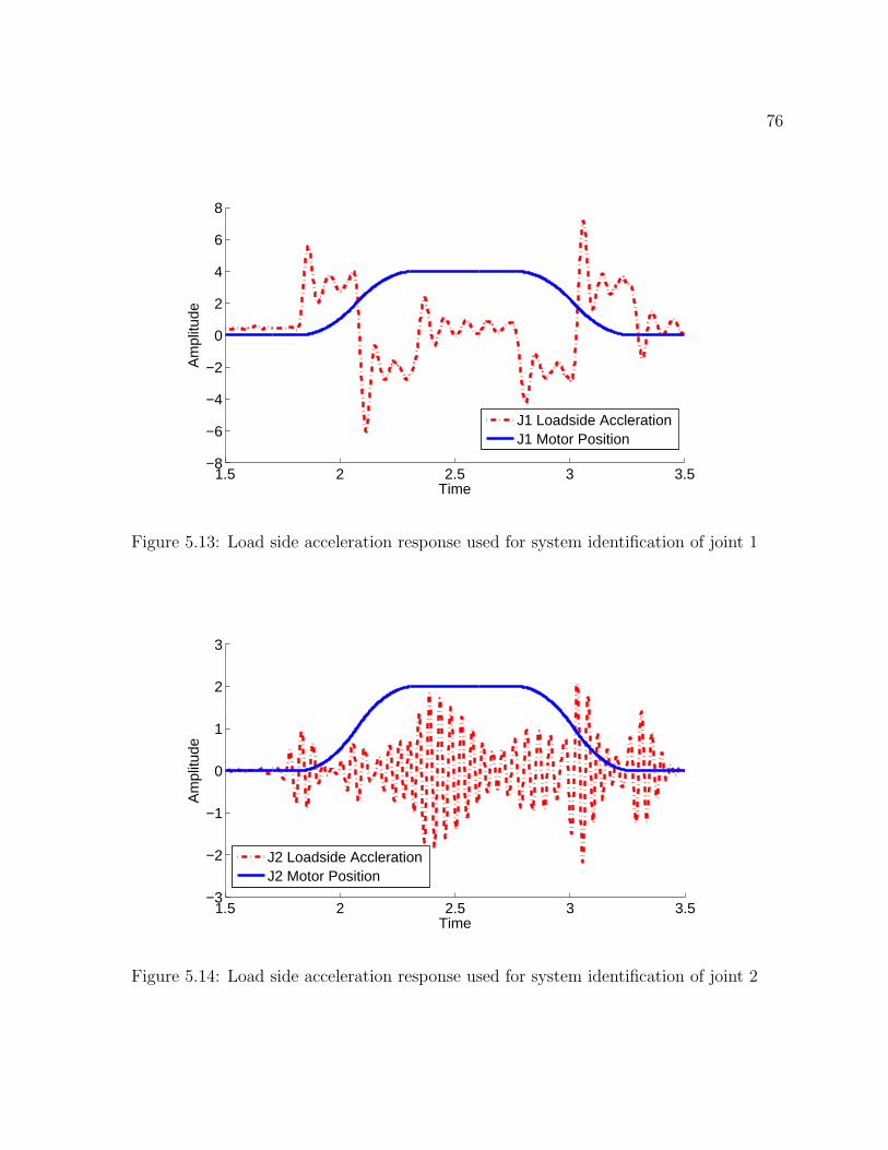
76

1.5 2 2.5 3 3.5−8

−6

−4

−2

0

2

4

6

8

Time

Am

plitu

de

J1 Loadside AcclerationJ1 Motor Position

Figure 5.13: Load side acceleration response used for system identification of joint 1

1.5 2 2.5 3 3.5−3

−2

−1

0

1

2

3

Time

Am

plitu

de



77

1.5 2 2.5 3 3.5−6

−4

−2

0

2

4

6A

mpl

itude

Time (sec)



2.95 3 3.05 3.1 3.15 3.2

0

10

20x 10

−3

Am

plitu

de

Load side position Comparison


1.5 2 2.5 3 3.5−0.01

0

0.01

0.02

Time (Seconds)

Am

plitu

de


Figure 5.16: Compensated response: top subplot shows the load side position trackingperformance, bottom subplot shows load side error

78

6.8 7 7.2 7.4 7.6 7.8 8−2

−1

0

1

2

3

4

5x 10

−3

Time (seconds)

Rad

ians

TCP Position Error Comparison

TCP X−Axis Error Post CompTCP X−Axis Error Pre Comp

Figure 5.17: Compensated response: load side position tracking error along X axis

6.8 7 7.2 7.4 7.6 7.8 8

−5

0

5

10

x 10−3

Time (seconds)

Rad

ians


TCP Y−Axis Error Post CompTCP Y−Axis Error Pre Comp

Figure 5.18: Compensated response: load side position tracking error along Y axis

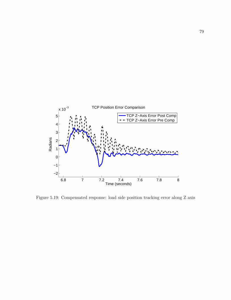
79

6.8 7 7.2 7.4 7.6 7.8 8

−2

−1

0

1

2

3

4

5

x 10−3

Time (seconds)

Rad

ians


TCP Z−Axis Error Post CompTCP Z−Axis Error Pre Comp

Figure 5.19: Compensated response: load side position tracking error along Z axis

80

Chapter 6

Conclusions

6.1 Chapter Summary

This dissertation presented feedback and feedforward controller design techniques for directapplication to industrial robots. Chapter 2 introduced the background information necessaryto understand this dissertation. This information includes single joint modeling techniques,multi joint robot dynamics, and controller structure. This chapter also introduced the soft-ware and hardware used for experimental verification in this dissertation as well as relevantsystem identification results.

Chapter 3 presented an algorithm for automatic gain tuning of robot manipulators. Theproposed approach is an iterative method that uses nonlinear programming to improve robotperformance by successively reducing a cost function. This chapter also discusses barriermethods, stepsize selection, as well as initial gain selection. Experimental results are includedto verify the effectiveness of the proposed approach.

Chapter 4 presents a controller framework based on the disturbance observer. This con-troller framework is designed for gain tuning purposes and is shown to be robustly stableunder a few mild assumptions. These assumptions are addressed and do not hinder the pro-posed framework’s viability for most gain tuning scenarios. The framework is experimentallyshown to be stable under a large range of controller gain variations.

Chapter 5 introduces an input shaping approach for reducing residual vibrations in in-dustrial robots with joint flexibilities. This approach models the joint dynamics as a simplesecond order system and utilizes a simple system identification process to identify the modelparameters. Experimental results show that the proposed approach is effective at reducingresidual vibrations in robot manipulators, especially when the link inertia is large.

81

6.2 Future Work

Additional research can be done to further improve the topics presented in this dissertation.Chapter 3 presented an algorithm for automatically tuning the feedback controller gain forrobot manipulators. Further work can be done to improve the step size selection process.Additionally, the proposed gain tuning algorithm improves robot performance by iterativelyreducing a cost function. More work can be done to refine the cost function design process tosee how different cost function parameters correlate to actual robot performance. Chapter 4presents a controller tuning framework for stable gain tuning. The proposed framework canuse further experimental verification. In particular, it would be interesting to combine theproposed gain tuning algorithm from chapter 3 with the framework proposed in chapter 4.More specifically, it would be interesting to tune the free controller Ct(s) in the DOB frame-work using the proposed gain tuning approach presented in chapter 3. And finally, chapter 5presented an input shaping method for suppressing residual joint vibrations. The currentimplementation assumes good motor side performance, which is something that is not alwaysreadily available. More work can be done to extend the input shaping approach to situationswhere the motor feedback controller has not been optimized.

82

Bibliography

[1] Analog Devices Inc. www.analog.com/en/mems-sensors/imu/adis16400/products/product.html.

[2] Kartik B. Ariyur and Miroslav Krstic. Real-Time Optimization by Extremum-SeekingControl. John Wiley & Sons, 2003.

[3] K. Astrom and T. Hagglund. PID Controllers: Theory, Design, and Tuning. TheInternational Society for Measurement and Control, 2nd edition, 1995.

[4] Dimitri P. Bertsekas. Nonlinear Programming. Athena Scientific, 2nd edition, 2008.

[5] Stephen Boyd and Lieven Vandenberghe. Convex Optimization. Cambridge UniversityPress, 2008.

[6] D. Bristow, M. Tharayil, and A. Alleyne. A survey of iterative learning control. IEEEControl Systems, 26:96–114, 2006.

[7] Michael Chan, Kyoungchul Kong, and Masayoshi Tomizuka. Automatic controller gaintuning of a multiple joint robot based on modified extremum seeking control. Proceedingsof the 18th IFAC World Congress, pages 4131–4136, 2011.

[8] Wenjie Chen. Intelligent Control of Robots with Midmatched Dynamics and MismatchedSensing. PhD thesis, 2012.

[9] Wenjie Chen, Pedro Reynoso Mora, Mike Chan, Cheng-Huei Han, and MasayoshiTomizuka. UCB-FANUC Project: Activity Report June 2009 May 2010. Techni-cal report, Mechanical Engineering Department, University of California, Berkeley.

[10] Wenjie Chen, Pedro Reynoso Mora, Mike Chan, Cong Wang, Chung-Yen Lin, andMasayoshi Tomizuka. UCB-FANUC Project: Activity Report June 2011 May 2012.Technical report, Mechanical Engineering Department, University of California, Berke-ley.

[11] Wenjie Chen, Pedro Reynoso Mora, Mike Chan, Cong Wang, and Masayoshi Tomizuka.UCB-FANUC Project: Activity Report June 2010 May 2011. Technical report, Me-chanical Engineering Department, University of California, Berkeley.

83

[12] CompuGauge 3D. www.dynalog-us.com/solutions/.

[13] P. Corke. A robotics toolbox for MATLAB. IEEE Robotics and Automation Magazine,3:24–32, 1996.

[14] FANUC Corp. www.micromech.co.uk/dir products/pdf/fanuc/m 16ib 20 10l.pdf.

[15] Gene F. Franklin, J. David Powell, and Abbas Emami-Naeini. Feedback Control ofDynamic Systems. Pearson Prentice Hall, 5th edition, 2006.

[16] Fathi Ghorbel, John Y. Hung, and Mark W. Spong. Adaptive control of flexible-jointmanipulators. Control Systems Magazine, 9:9–13, 1989.

[17] I. Godler, K. Ohnishi, and T. Yamashita. Repetitive control to reduce spped ripplecaused by strain wave gearing. Internation Conference on Industrial Electronics, Controland Instrumentations, 2:1034–1038, 1994.

[18] Cheng-Huei Han, Wenjie Chen, Pedro Reynoso Mora, Mike Chan, and MasayoshiTomizuka. UCB-FANUC Project: Activity Report June 2008 May 2009. Techni-cal report, Mechanical Engineering Department, University of California, Berkeley.

[19] Cheng-Huei Han, Kyoungchul Kong, and Masayoshi Tomizuka. Sensor-based controllertuning of robot manipulators by real-time optimization. Proc. of 9th InternationalSymposium on Robot Control (SYROCO), pages 715–720, 2009.

[20] Cheng-Huei Han, Chun-Chih Wang, and Masayoshi Tomizuka. Suppression of vibrationdue to transmission error of harmonic drives using peak filter with acceleration feedback.IEEE International Workshop on Advanced Motion Control, pages 182–187, 2008.

[21] HarmonicDrive. http://www.harmonicdrive.net/.

[22] Monson H. Hayes. Statistical Digital Signal Processing and Modeling. John Wiley &Sons, 1996.

[23] S. Kemal Ider and Ozan Korkmaz. Trajectory tracking control of parallel robots in thepresence of joint drive flexibility. Journal of Sound and Vibration, 319:77–90, 2009.

[24] Kyoungchul Kong, Kiyonori Inaba, and Masayoshi Tomizuka. Real-time nonlinear pro-gramming by amplitude modulation. Proc. of ASME Dynamics Systems and ControlConference, pages 417–424, 2008.

[25] Lennart Ljung. System Identification: Theory for the User. PTR Prentice Hall Infor-mation and System Sciences Series. Prentice Hall PTR, 2nd edition, 1999.

84

[26] David G. Luenberger. Linear and Nonlinear Programming. International Series inOperations Research and Management Science. Springer Science+Business Media, 2ndedition, 2008.

[27] T. Marilier and J. A. Richard. Non-linear mechanic and electric behavior of a robotaxis with a “harmonic-drive” gear. Robotics and Computer-Integrated Manufacturing,5:129–136.

[28] MATLAB. www.mathworks.com/products/index.html.

[29] Leonard Meirovitch. Fundamental of Vibrations. McGRAW-HILL INTERNATIONEDITIONS: Mechanical Engineering Series. McGraw-Hill Higher Education, 2001.

[30] C. Walton Musser. Strain Wave Gear-Species in Which Only One of the Gears is Input.

[31] National Instruments. www.ni.com/labview/.

[32] Alan V. Oppenheim and Ronald W. Schafer. Discrete-Time Signal Processing. PrenticeHall Signal Processing Series. Prentice Hall, 3rd edition, 2010.

[33] Neil Sclater. Mechanisms and Mechanical Devices Sourcebook. McGraw-Hill, 5th edition,2011.

[34] Nabesco RV Series Spec Sheet. www.nabtescomotioncontrol.com/pdfs/rvseries.pdf.

[35] Bruno Siciliano, Lorenzo Sciavicco, Luigi Villani, and Giuseppe Oriolo. Robotics: Mod-elling, Planning and Control. Advanced Textbooks in Control and Signal Processing.Springer, 2009.

[36] N. Singer and W. Seering. Preshaping command inputs to reduce system vibration.Journal of Dynamic Systems, Measurement, and Control, 112:76–82, 1997.

[37] S. Skogestad and I. Postlethwaite. Multivariable Feedback Control, Analysis, and Design.John Wiley & Sons, 2005.

[38] Timothy D. Tuttle. Understanding and Modeling the Behavior of a Harmonic DriveGear Transmission. Technical report, MIT Artificial Intelligence Laboratory.

[39] Chun-Chih Wang. Motion control of Indirect-drive Robots: Model Based ControllerDesign and Performance Enhancement Based on Load-side Sensors. PhD thesis, 2008.

[40] Chun-Chih Wang and Masayoshi Tomizuka. Sensor-based controller tuning of indirectdrive trains. Advanced Motion Control, pages 188–193, 2008.

[41] G. Zames. On the input-output stability of time-varying nonlinear feedback systemspart one: Conditions derived using concepts of loop gain, conicity, and positivity. IEEETransactions on Automatic Control, 11:228–238, 1966.

controller synthesis and vibration suppression...

Documents