controller optimization with constraints on probabilistic...

Structural Engineering and Mechanics, Vol. 17, No. 3-4 (2004) 593-609 593

Controller optimization with constraints on probabilistic peak responses

Ji-Hun Park†

MIDASIT Co., Ltd., Seoul, Korea

Kyung-Won Min‡

Department of Architectural Engineering, Dankook University, Seoul, Korea

Hong-Gun Park‡

Department of Architecture, Seoul National University, Korea

(Received January 6, 2003, Accepted August 8, 2003)

Abstract. Peak response is a more suitable index than mean response in the light of structural safety. Inthis study, a controller optimization method is proposed to restrict peak responses of building structuressubject to earthquake excitations, which are modeled as partially stationary stochastic process. Theconstraints are given with specified failure probabilities of peak responses. LQR is chosen to assurestability in numerical process of optimization. Optimization problem is formulated with weightings oncontrolled outputs as design variables and gradients of objective and constraint functions are derived. Fullstate feedback controllers designed by the proposed method satisfy various design objectives and outputfeedback controllers using LQG also yield similar results without significant performance deterioration.

Key words: stochastic process; crossing rate; failure probability; optimization; linear quadratic regulator.

1. Introduction

Many active structural control methods have been developed and implemented in the field of civilengineering to suppress excessive vibrations induced by earthquake or wind loads (Soong 1990,Housner et al. 1997). Due to the nature of such loads, their magnitudes and distributions cannot beexactly specified, but can be defined stochastically only. Therefore, the quantification of controleffectiveness based on probabilistic concept is an important problem in controller design. Standarddeviation is the most commonly used response quantity for stochastically excited structures, becausemost random disturbances can be approximated by white or filtered white noises and the responsecovariance matrix of a linear time invariant (LTI) system under a white noise excitation can beobtained by solving a Lyapunov equation. Further, the exact probability distribution of peakresponses is not known (Lutes and Sarkani 1997). Accordingly, widely used control methodologies

† Senior Developer‡ Professor

594 Ji-Hun Park, Kyung-Won Min and Hong-Gun Park

such as Linear Quadratic Regulator (LQR) and Linear Quadratic Gaussian (LQG) control algorithmsminimize the standard deviation of responses. However, in the light of structural safety, the criticalresponse quantity is defined as a peak value rather than a standard deviation.

Spencer et al. (1994a) proposed a probabilistic controller design method for a single degree offreedom (SDF) structure considering the uncertainty in structural parameters. In their research, theprobability of peak displacements exceeding critical value is used as an objective function and theroot mean square (RMS) value of control forces is used as a constraint. May and Beck (1998)investigated an unconstrained optimization of the acceleration feedback controller for a three-storytest building structure taking into account the parameter uncertainty in ground accelerationmodeling. They minimized the failure probability defined by a safe region, but the level of thefailure probability could not be specified. An important problem in the controller optimization isthat a control gain may fall into an unstable region while seeking an optimal solution. In such cases,the probability distribution of the closed-loop system does not exist and the optimization processcannot be continued, since the closed-loop system responses diverge. In the previous two studies bySpencer et al. and May and Beck, there were no remarks on this issue. This is because the simplecontroller structures that they used make it easy to set up constraints on the stability.

There have been a lot of studies on controller optimization of which solution has the form of LQRcontroller. This is due to the facts that LQR controller has a simple stability condition expressed interms of weightings on output variables, and that it can be easily extended to an output feedbackcontroller with an appropriate observer, for example, LQG controller with Kalman filter. Studies onLQR or LQG controller optimization can be classified into three groups. First, Hsieh et al. (1989)and Zhu et al. (1997) studied the optimization with constraints on the covariance of outputvariables. Second, Zhu and Skelton (1991) and Rotea (1993) studied the optimization withconstraints on L∞ norm of output variables, which is deterministic norm and may be tooconservative. Third, Toivonen and Mäkilä (1989) and Khargonekar and Rotea (1991) studied theoptimization problem with multiple objective functions on RMS values of output variables. Butnone of them dealt with optimization with constraints on the probabilistic peak values of outputvariables considering the stochastic nature of external loads.

In this paper, a new controller optimization method is proposed to restrict the failure probabilitiesof peak responses below specified levels with minimum control force for multi degree of freedom(MDF) structures. The optimization problem is formulated with weightings on controlled responsesas design variables. Gradients of objective function and inequality constraints are derived to makeuse of general gradient based optimization algorithms. The limit in the actuator stroke is alsoconsidered in the optimization problem. LQR controller with full state feedback is first chosen as asubject controller to deal with more complex and general controller types for MDF structures and toestablish simple stability conditions. Next, the optimized full state feedback controller is extended tothe output feedback controller using LQG with Kalman filters. The performance degradation due tothe output feedback is evaluated in the numerical examples.

2. Problem statements

2.1 Augmented design plant

The augmented design plant is composed of a building structure, a control device and a

Controller optimization with constraints on probabilistic peak responses 595

disturbance frequency shaping filter. Each floor of the structure is assumed to have a diaphragmconstraint so that the number of degree of freedom is equal to that of floors through staticcondensation and ignoring vertical deformations. The control device considered in this paper is ahybrid mass damper (HMD) that works as a tuned mass damper (TMD) for low level vibrations andas an active tuned mass damper (ATMD) for high level vibrations. The state space representation ofthe equation of motion for an n degree of freedom structure with a HMD is

(1)

(2)

where

(3)

and xs, ys, fg and u are, respectively, the (2n + 2) state vector, the (2n + 1) vector of controlledresponses, the ground acceleration, and the control force, and q, qd, , and qd, HMD are,respectively, the (n + 1) vector of relative displacements of floors and the HMD, the n inter-storydrift vector, the n absolute floor acceleration vector, and the HMD stroke. As, Bs1, Bs2, Cs1, and Ds1

are the state matrix, the disturbance influence matrix, the control force influence matrix, the outputmatrix, and the matrix that represents the coupling between the control force and controlledresponses, respectively.

The actuator dynamics is mathematically modeled with a first-order low pass filter (Yang et al.1996) and represented by the following state space equation.

(4)

(5)

where v, xa, and ωa are the control signal expressed as input voltage, the state of the actuator, thecut-off frequency, respectively, and αa is a constant. The state space representation of Kanai-Tajimifilter is used for the frequency shaping filter of the ground acceleration.

(6)

(7)

where

(8)

x·s Asxs Bs1 fg Bs2u+ +=

ys Cs1xs Ds1u+=

xsq

q·; ys

qd

q··ab

qd HMD,

==

q··ab

x·a ωaxa– ωav+=

u αaxa=

x·f Af xf Bfw+=

fg Cf xf=

xfqf

q·f

; Af0 1

ωg2 – 2ξgωg–

= ; Bf0

1–= ; Cf ωg

2– 2ξgωg–[ ]==


and xf, w, qf, ωg, and ξg are the state vector of the filter, the input white noise of the filter, therelative displacement of Kanai-Tajimi filter, the natural frequency of the filter, and the damping ratioof the filter, respectively. If soil property data is lack, a low pass filter, which is represented by thesame state space equation form of Eqs. (6) and (7), can be used (Spencer et al. 1994b).

In sum, the augmented design plant for the structure with a HMD, the actuator, and the frequencyshaping filter of ground acceleration is given as

(9)

(10)

where

(11)

(12)

where x is the (2n + 5) state vector, y is the (2n + 3) vector of output variables, and O and 0 are azero matrix and a zero vector with appropriate dimensions. To represent the non-stationary propertyof earthquake, the envelope function proposed by Jennings et al. (1968) is multiplied to the whitenoise input, w, in the above augmented plant equations. A resulting sample ground acceleration anda scaled envelope function is presented in Fig. 1.

x· Ax B1w B2v+ +=

y Cx Dv+=

xxs

xa

xf

; AAs Bs2αa Bs1Cf

O ωa O

O O Af

= ; B1

00Bf

; B2

0ωa

0

===

yys

u

v

= ; CCs1 Ds1αa O

O αa O

O O O

; D001

==

Fig. 1 Sample ground acceleration and the shape of envelope function


2.2 Definition of peak response

From the viewpoint of safety and economy, it is required to specify the probability that the peakresponse exceeds prescribed critical value. Peak response can be expressed stochastically using afailure probability, which is the probability that the controlled response of the system exceeds thecritical value. If the process X is stationary and Gaussian and the failure probability at the initialtime is zero, the failure probability of X is defined as the probability that |X | exceeds a prescribedbarrier level b during the interval, tb, and is approximately given as (Lutes and Sarkani 1997)

(13)

where is the X’s crossing rate. The crossing rate is defined as an average number of |X |exceeding a prescribed level, b, during a unit time interval and expressed as

(14)

where σX and are, respectively, standard deviations of process X and its time derivative (Lutes andSarkani 1997).

Since the envelope function is flat for its largest amplitude part, the strong ground motion,presented in Fig. 1, can be assumed to be a stationary Gaussian process based on the assumptionthat the influence of the non-stationarity of the ground motion at the early rising stage is small andcan be neglected. Since the steady-state output of a linear system subjected to the stationaryGaussian random excitation is also stationary and Gaussian, the plant output can be treated as astationary and Gaussian process during the strong excitation interval for elastic structures and linearcontrollers. Accordingly, the above equations are applied for the remaining parts of this paper inspite of non-stationarity of earthquake and corresponding structural responses. Otherwise, atechnique using evolutionary spectral density can be employed (Lin and Cai 1995), which is beyondthe scope of this paper and reserved as a future research topic.

2.3 Control algorithm

Control algorithms can be classified into full state feedback control algorithms and outputfeedback control algorithms. The former employs the complete information of the plant state whilethe latter employs limited information. Therefore, the full state feedback control is moreadvantageous than the output feedback control. For practical reason, however, all state variablescannot be measured and an observer is often used to estimate state variables with limited number ofmeasured responses. In this paper, only the optimization of the full state feedback controller ispresented, but, if the state estimation error is negligible, an observer can be added based on thewell-known separation principle (Burl 1999).

A full state feedback controller can be designed by optimizing the feedback control gain. Howeverthis process may cause instability of the closed loop system while seeking an optimum solution. Insuch case, the optimization cannot be continued since it becomes impossible to compute the normof diverging responses. To overcome this drawback, the feedback gain needs to be restricted withinthe safe range that feedback gains stabilize the plant. But, for multi-variable systems, it is difficult toset up clear stability conditions involving the feedback gain itself. To solve such problem, this study

P b tb,( ) 1 exp η X+ b( )– tb⋅[ ]–=

η X+ b( )

η X+ b( )

σX·

πσX

---------expb2–

2σX2

---------

=

σX·


adopts LQR because the positive semi-definite state weighting matrix and the positive definitecontrol weighting matrix in its quadratic performance index always give stabilizing feedback gains.

For the output feedback control algorithm, LQG controller is investigated in this paper. In LQG,which is composed of LQR controller and Kalman filter, the plant disturbances and measurementnoises are modeled by white noises. Further, plant disturbances and all measurement noises areassumed to be uncorrelated.

3. Formulation of optimization problem

3.1 Optimization problem

For the controller optimization, the variance of control force is selected as an objective function.That is, the optimization problem finds a control gain that requires a minimum control force in themean sense. Constraints on controlled outputs - inter-story drifts, absolute floor accelerations, andHMD stroke - are given as specified levels of corresponding failure probabilities. The control forceand control signal have no constraints, because if they are constrained, it may be impossible to finda controller satisfying constraints on structural responses. From optimization results, the peakcontrol force and signal defined with specified failure probabilities can be calculated.

The nonlinear constrained optimization problem is defined as

minimize (15)

subject to (16)

where is the variance of the control force that is the (2n + 2)-th output variable of Eq. (12)and S is a (2n + 3) by (2n + 3) matrix containing design variables which are weightings in theperformance index of LQR given by

(17)

in which

(18)

In Eq. (16), is the crossing rate of the k-th measured response, yk, over the barrier level bk,ts is the duration of stationary strong ground motion, and Pk is the pre-specified failure probabilityfor yk.

In order to reduce the number of design variables to 2n + 3, S is assumed to have a diagonalmatrix form as follows.

(19)

For the controller optimization, the weighting on the control signal, s2n+3, is set to be 1.0 andexcluded from the design variables, since the LQR control gain depends on the relative valuesbetween weightings.

f S( ) Vy2n 2+=

gk S( ) 1 exp η yk

+ bk( )ts–[ ] Pk 0≤–– k 1 … 2n 1+, ,=,=

Vy2n 2+

J yTSydt0

∞∫ xTQx 2xTNv Rv2+ +( )dt

0

∞∫= =

Q CTSC; N CTSD; R DTSD===

η yk

+ bk( )

S diag s12

s22 … s2n 3+

2, , ,[ ]=


The failure probability of each output variable is determined by the crossing rate over the durationof stationary process. Because there is one-to-one relationship between the crossing rate and thefailure probability given by Eq. (13), the constraint Eq. (16) can be converted into the followingnonlinear inequality equations.

(20)

where and are variances of yk and , respectively, and ρk is an upper bound of crossingrate calculated from the Pk of Eq. (16) and the basic relationship of Eq. (13).

The optimal control gain, G, of LQR for a linear system under a Gaussian white noise disturbanceis known to be independent of the disturbance (Burl 1999) and given by

(21)

where P is the Riccati matrix, which can be calculated from the algebraic Ricatti equation(Anderson and Moore 1989)

(22)

In order to calculate the objective function and constraints, the covariance matrices of y and need to be obtained. The covariance matrix of the output vector y is calculated from a Lyapunovequation of the closed loop system (Burl 1999), and given as

(23)

subject to

(24)

where

(25)

and and are, respectively, the covariance matrices of state vector x and output vector y, andSw is the power spectral density (PSD) of the white noise disturbance.

The derivative of the output vector y can be written by

(26)

It can be seen in Eq. (26) that is a linear combination of the state vector and the white noisedisturbance. Since the state of LTI system under a white noise input is the Markov process, the statevector x and the white noise disturbance w in Eq. (26) are independent each other. Consequently,

gk S( )Vy·k

π Vykexp

bk2

2Vyk

----------

----------------------------------------- ρk– 0, k 1 … 2n 1+, ,=≤=

VykVy·k

y·k

G R1– B2

TP NT+( )=

PA ATP PB2 N+( )R 1– PB2 N+( )T– Q+ + O=

y·

Σyy CcΣxxCcT=

AcΣxx ΣxxAcT 2πSwB1B1

T+ + O=

Ac A B2G; Cc C DG–=–=

Σxx Σyy

y· Ccx· CcAcx CcB1w+= =

y·


the covariance matrix of is obtained as

(27)

where δ (0) is a Dirac delta function having an infinite value at zero. To avoid an infinite covariancematrix, the white noise disturbance is assumed to be band-limited. This can be justified because, forreal implementation of control problem, all signals are discretely represented with a sampling time,and frequency contents of those discrete signals higher than the Nyquist frequency are filtered out.In this study, the finite covariance matrix of is calculated using a basic conversion rule (Burl1999) between the variance of a continuous signal and its discrete counterpart as

(28)

where ∆t is the sampling time.

3.2 Gradients of objective function and inequality constraints

Algorithms to solve a nonlinear constrained optimization problem are grouped into gradient basedmethods and direct search methods. For the problem with large number of design variables, theformer is known to be more effective than the latter if the gradients of objective function andconstraints are continuous (Belegundu and Chandrupatla 1999). Accordingly, a gradient basedmethod is adopted in this paper, and the gradient calculations necessary in the optimizationprocedure are derived in this section.

The gradients of the objective function and the k-th constraint with respect to the p-th designvariable sp in Eq. (19) are obtained using chain rule such that

(29)

(30)

The derivative of the k-th constraint with respect to the corresponding variances and in the above equation can be obtained by simple differentiation. The derivatives of and withrespect to the p-th design variable sp can be obtained using the elements of Riccati matrix P andapplying the chain rule as

(31)

(32)

where Pij is the (i, j)-th component of P.

y·

Σy·y· Cc AcΣxxAcT 2πSwδ 0( )B1B1

T+[ ]CcT=

y·

Σy·y· Cc AcΣxxAcT 2πSw

t∆------------B1B1

T+ CcT=

∂f ·( )∂sp

-----------∂Vy2n 2+

∂sp

----------------=

∂gk ·( )∂sp

--------------∂gk ·( )∂Vyk

--------------∂Vyk

∂sp

----------∂gk ·( )∂Vy·k

--------------∂Vy·k

∂sp

----------, k+ 1 … 2n 1+, ,= =

gk ·( ) VykVy·k

VykVy·k

∂Vyk

∂sp

---------∂Vyk

∂Pij

---------∂Pij

∂sp

---------j 1=

2n 5+

∑i 1=

2n 5+

∑∂Σyy

∂Pij

----------kk

∂P∂sp

-------ijj 1=

2n 5+

∑i 1=

2n 5+

∑= = k 1 … 2n 1+, ,=

∂Vy·k

∂sp

----------∂Vy·k

∂Pi j

----------∂Pi j

∂sp

---------j 1=

2n 5+

∑i 1=

2n 5+

∑∂Σy·y·

∂Pi j

----------kk

∂P∂sp

-------ijj 1=

2n 5+

∑i 1=

2n 5+

∑= = k 1 … 2n 1+, ,=


The derivatives of the covariance matrices of y and , with respect to the component Pij in Eqs.(31) and (32) are obtained by partially differentiating Eqs. (23) and (28) with respect to Pij as

(33)

(34)

The derivatives of the matrices Ac and Cc with respect to the component Pij in Eqs. (33) and (34)are calculated as

(35)

(36)

where

(37)

The derivative of the covariance of the state vector with respect to the Riccati matrix, , inEqs. (33) and (34) is obtained by solving the following Lyapunov equation, which is derived bydifferentiating the Lyapunov equation (24) with respect to Pij.

(38)

The derivative of the Riccati matrix with respect to the p-th component of the weighting matrix sp,, is obtained by solving the following Lyapunov equation, which is obtained by

differentiating the Riccati Eq. (22) with respect to sp

(39)

where

(40)

Since the state space equation of the actuator is strictly proper and its number of state is one asshown in Eq. (4), only one component is non-zero in the matrix B2 of Eq. (11). In this case,

y·

∂Σyy

∂Pi j

----------∂Cc

∂Pi j

---------ΣxxCcT Cc

∂Σxx

∂Pi j

-----------CcT CcΣxx

∂CcT

∂Pi j

---------+ +=

∂Σy·y·

∂Pi j

----------∂Cc

∂Pi j

--------- AcΣxxAcT 2πSw

t∆------------B1B1+

CcT=

Cc

∂Ac

∂Pi j

---------ΣxxAcT Ac

∂Σxx

∂Pi j

-----------AcT AcΣxx

∂AcT

∂Pi j

---------+ + Cc

T+

Cc AcΣxxAcT 2πSw

t∆------------B1B1+

∂CcT

∂Pi j

---------+

∂Ac

∂Pi j

--------- B2R1– B2

T ∂P∂Pi j

---------–=

∂Cc

∂Pi j

--------- DR 1– B2T ∂P∂Pi j

---------–=

∂P∂Pi j

---------kl

1 if k i and l j==( )0 otherwise

=

∂Σxx ∂Pi j⁄

Ac

∂Σxx

∂Pi j

-----------∂Σxx

∂Pi j

-----------AcT ∂Ac

∂Pi j

---------Σxx Σxx

∂AcT

∂Pi j

---------+ + + 0=

∂P ∂sp⁄

∂P∂sp

-------Ac AcT ∂P∂sp

------- DG C–( )T ∂S∂sp

------- DG C–( )+ + 0=

∂S∂sp

-------i j

2sp if i j p= =( )

0 otherwise

=


in Eqs. (35) and in Eq. (36) are non-zero matrix only for i = 2n + 3 and j = 1,2, …. , 2n + 5. Therefore, only 2n + 5 of both ’s in Eq. (33) and ’s in Eq. (34)need to be calculated and the rest are zero. Further, Eqs. (35) and (36) are calculated only onceduring the entire optimization process because R is a fixed weighting for the control signal.

4. Numerical analysis

A ten-story shear building shown in Fig. 2 is used for the numerical analysis using the proposedoptimization process. The order of the design plant is 25. The larger the DOF of the structurebecomes, the more difficult convergence is. But, in many cases, this may not be a problem sincemost civil structural vibration is dominated by only a few modes and the design plants identifiedfrom experiments have small order.

Structural properties are presented in Table 1. The HMD installed on the top floor consists of aTMD and a hydraulic actuator. The mass of the TMD is 0.5% of the total mass of the building. Thenatural frequency and damping ratio of the TMD are determined from the equation proposed byAyorinde (Ayorinde and Warburton 1980) for optimal passive control.

∂Ac ∂Pi j⁄ ∂Cc ∂Pi j⁄∂Σxx ∂Pi j⁄ ∂Σy·y· ∂Pi j⁄

Fig. 2 Example ten-story shear building with a hybrid mass damper


Parameters used for the Kanai-Tajimi filter, the envelope function of the filter input, and theactuator model are presented in Table 2. The PSD of the white noise input, Sw, for the Kanai-Tajimifilter is determined to set the mean peak ground acceleration to 0.1 g from 1000 samples. Parametersof the envelope function are selected such that the strong motion continues stationarily from t1 to t2with falloff parameter c (Jennings et al. 1968).

Design variables are given by

(41)

where diagonal elements represents weightings on measured responses, which correspond to teninter-story drifts, ten absolute floor accelerations, an HMD stroke, a control force, and a controlsignal, respectively. As previously mentioned, the weighting on the control signal is set to be 1. Inorder to avoid an ill-conditioning and improve the optimization performance, scale factors of 1002,1, 1, 0.012, 102 are multiplied to five groups of weightings in Eq. (41), because they have differentdimensions.

Three different constraints sets on inter-story drifts, absolute floor accelerations, and an HMDstroke are given in Table 3. They are classified as A, B, and C according to the level of the HMDstroke. The optimization is carried out using the sequential quadratic programming algorithm inMATLAB Optimization Tool Box (Coleman et al. 1999). All peak responses including the controlforce and control signal presented in the remaining parts of this paper are based on 5% failure

S diag sd 1,2 … sd 10,

2sa 1,

2 … sa 10,2

sm2

su2 1, , , , , , , ,[ ]=

Table 1 Structural parameters

Floor Mass (kg) Stiffness (kgf/cm) Natural frequencies (Hz) Damping ratio

1 24300 10000 0.420.02

for all structural modes

2, 3, 4 24300 8000 1.16 / 1.90 / 2.645, 6, 7 24300 7000 3.22 / 3.82 / 4.208, 9, 10 24300 5000 4.67 / 5.09 / 5.51

Table 2 Parameters of ground acceleration model and actuator

Ground acceleration

Mean peak ground acceleration 0.1 gPSD of white noise input 7.949 × 10−4 m2/sec3

Natural frequency of filter 15.6 rad/secDamping ratio of filter 0.6

Envelope function t1 = 20 sec, t2 = 40 sec, c = 0.15

Actuatorωa 11.94 rad/secαa 400

Table 3 Constraint sets on peak responses

Constraint set A B C

Inter-story drift 2 cm 2 cm 2 cmFloor absolute acceleration 0.2 g 0.2 g 0.2 g

HMD stroke 1.5 m 1.75 m 2 m


probability assuming that the duration of the stationary large response is the same as that of thestationary strong ground motion, i.e. from 20 to 40 sec.

4.1 Full state feedback controller design

The controller optimization is performed for two different cases and the results are presented inTable 4 with activated constraints shaded. In the first case, denoted as LQR(I), sd, i (i = 1 to 10), sa, i

(i = 1 to 10), sm and su in Eq. (41) are included in the LQR performance index. In the second case,denoted as LQR(II), only sd, 2, sa, 10, sm and su are included, because peak inter-story drift andabsolute floor acceleration occur in the second and tenth floor, respectively, without control. Initialvalues for sd, i (i = 1 to 10), sa, i (i = 1 to 10), sm and su are 100, 100, 100 and 1, respectively, for bothcases. Constraints on all of the inter-story drifts, the absolute floor accelerations, and the HMDstroke are imposed for both cases.

The constraints on controlled responses except the second inter-story drift and the tenth floorabsolute acceleration are not activated so that they are not presented in Table 4. It is observed thatthe peak responses and control force for LQR(I) and LQR(II) are not significantly different in spiteof the difference in the number of design variables. Additionally, LQR(II), where the smallernumber of design variables is used, converges faster than LQR(I). Consequently, only LQR(II) withfive design variables will be discussed hereafter.

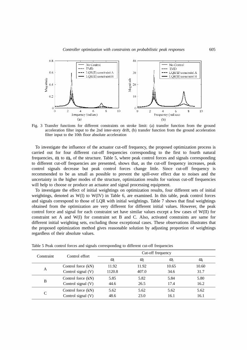
Table 4 indicates that a strict stroke constraint requires large control force. This is because theHMD is tuned to the first structural mode and limiting its stroke implies decreasing control effect onthat mode. When the stroke limit is not large enough for the first mode control, the control effortsmove onto higher modes to compensate consequent increase in overall responses. This requires largecontrol force since higher natural frequencies require the faster HMD movement. Fig. 3 shows theseesaw relation between responses of the first and second mode. That is, the LQR(II) withconstraint B (stroke = 1.75 m) is superior to LQR(II) with constraint A (stroke = 1.5 m) in controlof the first mode, while the latter with a smaller stroke limit is superior in control of the secondmode. For the optimization with a stroke constraint of 1.25 m, not presented in Table 4, no feasiblesolution is found. This means that there exists a lower limit of the stroke, which can be determinedfrom optimizations with different stroke constraints.

Table 4 Controlled peak responses (Activated constraints are shaded)

Controller Constraint2nd

inter-storyDrift (cm)

10th floor absolute acceleration

(g)

Stroke(m)

Control force(kN)

Control signal(V)

No control 3.67 0.30 · · ·

Passive control 2.70 0.26 1.41 · ·

LQR (I)A 2.00 0.18 1.50 10.74 37.4B 2.00 0.20 1.75 5.79 18.0C 2.00 0.20 1.92 5.69 17.8

LQR (II)A 2.00 0.18 1.50 10.65 34.6B 2.00 0.20 1.75 5.84 17.4C 2.00 0.20 1.93 5.62 16.1


To investigate the influence of the actuator cut-off frequency, the proposed optimization process iscarried out for four different cut-off frequencies corresponding to the first to fourth naturalfrequencies, ω1 to ω4, of the structure. Table 5, where peak control forces and signals correspondingto different cut-off frequencies are presented, shows that, as the cut-off frequency increases, peakcontrol signals decrease but peak control forces change little. Since cut-off frequency isrecommended to be as small as possible to prevent the spill-over effect due to noises and theuncertainty in the higher modes of the structure, optimization results for various cut-off frequencieswill help to choose or produce an actuator and signal processing equipment.

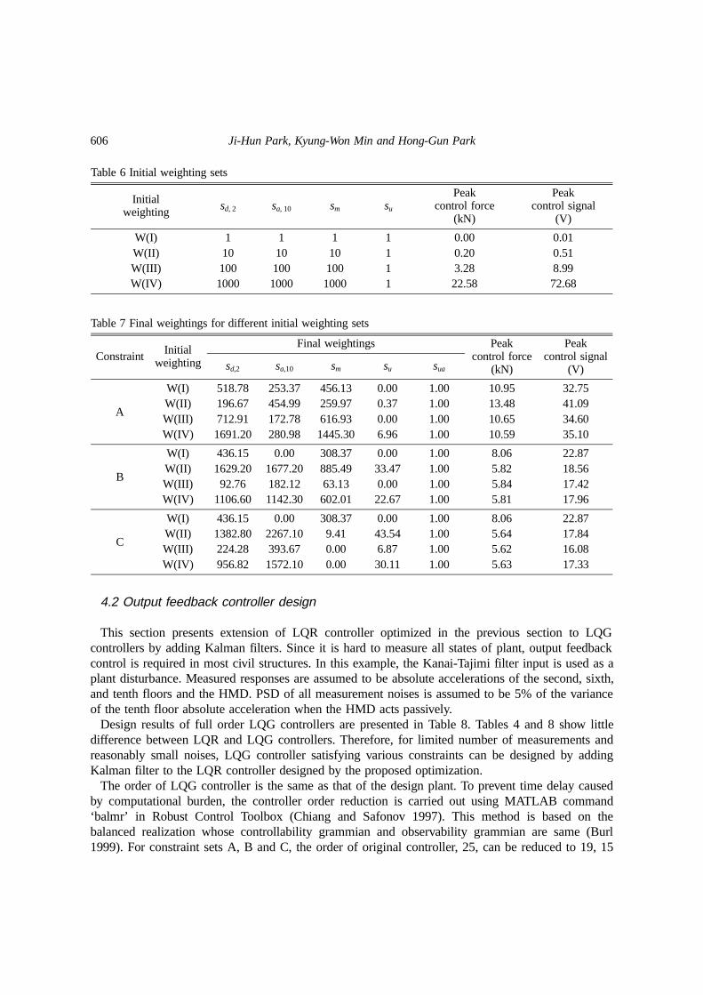
To investigate the effect of initial weightings on optimization results, four different sets of initialweightings, denoted as W(I) to W(IV) in Table 6, are examined. In this table, peak control forcesand signals correspond to those of LQR with initial weightings. Table 7 shows that final weightingsobtained from the optimization are very different for different initial values. However, the peakcontrol force and signal for each constraint set have similar values except a few cases of W(II) forconstraint set A and W(I) for constraint set B and C. Also, activated constraints are same fordifferent initial weighting sets, excluding those exceptional cases. These observations illustrates thatthe proposed optimization method gives reasonable solution by adjusting proportion of weightingsregardless of their absolute values.

Fig. 3 Transfer functions for different constraints on stroke limit: (a) transfer function from the groundacceleration filter input to the 2nd inter-story drift, (b) transfer function from the ground accelerationfilter input to the 10th floor absolute acceleration

Table 5 Peak control forces and signals corresponding to different cut-off frequencies

Constraint Control effortCut-off frequency

ω1 ω2 ω3 ω4

AControl force (kN) 11.92 11.92 10.65 10.60Control signal (V) 1120.8 407.0 34.6 31.7

BControl force (kN) 5.85 5.82 5.84 5.80Control signal (V) 44.6 26.5 17.4 16.2

CControl force (kN) 5.62 5.62 5.62 5.62Control signal (V) 48.6 23.0 16.1 16.1


4.2 Output feedback controller design

This section presents extension of LQR controller optimized in the previous section to LQGcontrollers by adding Kalman filters. Since it is hard to measure all states of plant, output feedbackcontrol is required in most civil structures. In this example, the Kanai-Tajimi filter input is used as aplant disturbance. Measured responses are assumed to be absolute accelerations of the second, sixth,and tenth floors and the HMD. PSD of all measurement noises is assumed to be 5% of the varianceof the tenth floor absolute acceleration when the HMD acts passively.

Design results of full order LQG controllers are presented in Table 8. Tables 4 and 8 show littledifference between LQR and LQG controllers. Therefore, for limited number of measurements andreasonably small noises, LQG controller satisfying various constraints can be designed by addingKalman filter to the LQR controller designed by the proposed optimization.

The order of LQG controller is the same as that of the design plant. To prevent time delay causedby computational burden, the controller order reduction is carried out using MATLAB command‘balmr’ in Robust Control Toolbox (Chiang and Safonov 1997). This method is based on thebalanced realization whose controllability grammian and observability grammian are same (Burl1999). For constraint sets A, B and C, the order of original controller, 25, can be reduced to 19, 15

Table 7 Final weightings for different initial weighting sets

Constraint Initial weighting

Final weightings Peakcontrol force

(kN)

Peakcontrol signal

(V)sd,2 sa,10 sm su sua

A

W(I) 518.78 253.37 456.13 0.00 1.00 10.95 32.75W(II) 196.67 454.99 259.97 0.37 1.00 13.48 41.09W(III) 712.91 172.78 616.93 0.00 1.00 10.65 34.60W(IV) 1691.20 280.98 1445.30 6.96 1.00 10.59 35.10

B

W(I) 436.15 0.00 308.37 0.00 1.00 8.06 22.87W(II) 1629.20 1677.20 885.49 33.47 1.00 5.82 18.56W(III) 92.76 182.12 63.13 0.00 1.00 5.84 17.42W(IV) 1106.60 1142.30 602.01 22.67 1.00 5.81 17.96

C

W(I) 436.15 0.00 308.37 0.00 1.00 8.06 22.87W(II) 1382.80 2267.10 9.41 43.54 1.00 5.64 17.84W(III) 224.28 393.67 0.00 6.87 1.00 5.62 16.08W(IV) 956.82 1572.10 0.00 30.11 1.00 5.63 17.33

Table 6 Initial weighting sets

Initialweighting sd, 2 sa, 10 sm su

Peakcontrol force

(kN)

Peakcontrol signal

(V)

W(I) 1 1 1 1 0.00 0.01W(II) 10 10 10 1 0.20 0.51W(III) 100 100 100 1 3.28 8.99W(IV) 1000 1000 1000 1 22.58 72.68


and 15, respectively. The peak responses with reduced LQG in Table 8 show insignificantperformance deterioration compared to those of full order LQG.

4.3 Verification of failure probability

Since the failure probability presented in Eq. (13) is an approximation, simulations using 1,000earthquake samples are performed to verify assumptions used in the proposed optimization method.Sample ground accelerations are generated by filtering white noises multiplied by the non-stationaryenvelope function through Kanai-Tajimi filter. Table 9, where the simulation result is presented,indicates that most failure probabilities of the activated constraints (distinguished by shade) are alittle smaller than 5%, which is the target value in the optimization. The reason is that structuralresponses do not reach to steady state at t1 = 20 sec., the beginning of stationary response assumedfor the calculation of failure probability, due to the initial non-stationarity of the earthquakeexcitation. For the future study, a design method addressing this effect needs to be developed formore accurate estimation of failure probability.

Table 8 Peak responses of LQG controllers

Controller Constraint2nd

inter-storydrift (cm)


(g)

Stroke(m)

Control force(kN)

Control signal(V)

No control 3.67 0.30 · · ·

Passive control 2.70 0.26 1.41 · ·

Full orderLQG

A 2.01 0.18 1.51 10.21 33.2B 2.00 0.20 1.75 5.83 17.4C 2.00 0.20 1.94 5.62 15.9

Reduced LQG

A 2.00 0.18 1.51 10.23 33.3B 2.00 0.20 1.75 5.88 17.7C 2.01 0.20 1.94 5.57 16.0

Table 9 Failure probability obtained from 1000 simulations

Constraint Controller2nd

inter-storydrift (cm)


(g)

Stroke(m)

Control force(kN)

Control signal(V)

ALQR ( II ) 4.1 0.9 3.9 4.6 4.1

LQG 4.1 0.8 3.9 4.6 3.1Reduced LQG 4.2 0.8 4.0 5.0 3.1

BLQR ( II ) 3.7 4.0 3.4 3.5 4.4

LQG 3.6 4.1 3.5 3.7 4.1Reduced LQG 3.6 4.2 3.6 3.7 4.1

CLQR ( II ) 4.7 4.2 1.5 5.4 3.7

LQG 4.6 4.2 1.6 5.3 5.0Reduced LQG 4.9 4.6 1.6 5.1 5.2


5. Conclusions

The present study proposes an optimal controller design method for the minimum control forcewith constraints on the failure probability of peak response. LQR is selected as control algorithm tokeep closed-loop system stable easily during optimization procedure. Gradients of objective functionand inequality constraints are derived to make use of general gradient based optimizationalgorithms.

Numerical analysis shows that the solution is not unique for various initial weightings. Butdifferent controllers, excluding a few exceptional results, show similar performance in terms of thepeak control force and responses. The effects of stroke limitation and actuator cut-off frequency oncontrol performance are investigated. It is observed that the strict constraint on stroke increases thepeak control force due to the tendency of controlling higher modes. Also, the reduction of actuatorcut-off frequency tends to increase the control signal rather than control force.

Performance degradation due to the output feedback using Kalman filter appended to theoptimized LQR controller is found to be negligible. Further, the additional performance degradationdue to the controller order reduction for LQG is not significant. Therefore, the proposedoptimization of LQR can be used to design a low order output feedback controller for a structurewith limited number of measured responses. Statistics of simulation results for 1,000 artificialearthquakes shows that failure probabilities of optimized control system are sufficiently accurate.

Acknowledgements

The work presented in this paper was partially supported by Research Fund of the NationalResearch Laboratory Program (Project No. M1-0203-00-0068) from the Ministry of Science andTechnology in Korea. The authors also gratefully acknowledge the support of this research by theSmart Infra-Structure Technology Center (SISTeC) (Project No. R11-2022-101-03004-0(2002)).

References

Anderson, B.D.O. and Moore, J.B. (1989), Optimal Control, Prentice Hall, Englewood Cliffs, NJ.Ayorinde, E.O. and Warburton, G.B. (1980), “Minimizing structural vibrations with absorbers”, Earthq. Eng.

Struct. Dyn., 8, 219-236.Belegundu, A.D. and Chandrupatla, T.R. (1999), Optimization Concepts and Applications in Engineering,

Prentice Hall, NJ.Burl, J.B. (1999), Linear Optimal Control, Addison-Wesley, CA.Chiang, R.Y. and Safonov, M.G. (1997), Robust Control Toolbox, The Math Works, Inc.Coleman, T., Branch, M.A. and Grace, A. (1999), Optimization Toolbox for Use with MATLAB, The Math

Works, Inc.Housner, G.W., Bergman, L.A., Caughey, T.K., Chassiakos, A.G., Claus, R.O., Masri, S.F., Skelton, R.E., Soong,

T.T., Spencer, B.F. Jr. and Yao, J.T.P. (1997), “Special issue structural control: past, present, and future”, J.Eng. Mech., ASCE, 123(9), 897-971.

Hsieh, C., Skelton, R.E. and Damra, F.M. (1989), “Minimum energy controllers with inequality constraints onoutput variances”, Optimal Control Applications & Methods, 10, 347-366.

Jennings, P.C., Housner, G.W. and Tsai, N.C. (1968), “Simulated earthquake motions”, Rept. Earthquake Eng.Res. Lab., California Institute of Technology.


Khargonekar, P.P. and Rotea, M.A. (1991), “Multiple objective optimal control of linear systems: The quadraticnorm case”, IEEE Transactions on Automatic Control, 36(1), 14-24.

Lin, Y.K. and Cai, G.Q. (1995), Probabilistic Structural Dynamics, McGraw-Hill, NY.Lutes, L.D. and Sarkani, S. (1997), Stochastic Analysis of Structural and Mechanical Vibrations, Prentice Hall,

NJ.May, B.S. and Beck, J.L. (1998), “Probabilistic control for the active mass driver benchmark structural model”,

Earthq. Eng. Struct. Dyn., 27, 1331-1346.Rotea, M.A. (1993), “The generalized H2 control problem”, Automatic, 29(2), 373-385.Soong, T.T. (1990), Active Structural Control: Theory and Practice, Longman Wiley, London.Spencer, B.F. Jr., Kaspari, D.C. and Sain, M.K. (1994a), “Structural control design: a reliability-based approach”,

Proc. of the American Control Conf., IEEE, 1062-1066.Spencer, B.F. Jr., Suhardjo, J. and Sain, M.K. (1994b), “Frequency domain optimal control strategies for seismic

protection”, J. Eng. Mech., ASCE, 120(1), 135-158.Toivonen, H.T. and Mäkilä, P.M. (1989), “Computer-aided design procedure for multi-objective LQG control

problems”, International Journal of Control, 49(2), 655-666.Yang, J.N., Wu, J.C., Reinhorn, A.M., Riley, M., Schmitendorf, W.E. and Jabbari, F. (1996), “Experimental

verification of H∞ and sliding mode control for seismically excited buildings”, J. Struct. Eng., 122(1), 69-75.Zhu, G. and Skelton, R. (1991), “Mixed L2 and L∞ problems by weight selection in quadratic optimal control”,

International Journal of Control, 53(5), 1161-1176.Zhu, G., Rotea, M.A. and Skelton, R. (1997), “A convergent algorithm for the output covariance constraint

control problem”, SIAM Journal of Control and Optimization, 35(1), 341-361.

controller optimization with constraints on probabilistic...

Documents