controlled sensitivity of marine controlled-source
TRANSCRIPT

CONTROLLED SENSITIVITY OF MARINE
CONTROLLED-SOURCE
ELECTROMAGNETIC
SURVEYS
by
Daeung Yoon
A thesis submitted to the faculty of The University of Utah
in partial fulfillment of the requirements for the degree of
Master of Science
in
Geophysics
Department of Geology and Geophysics
The University of Utah
May 2012

Copyright © Daeung Yoon 2012
All Rights Reserved

T h e U n i v e rs i t y o f U ta h Gra dua te S cho o l
STATEMENT OF THESIS APPROVAL
The thesis of Daeung Yoon
has been approved by the following supervisory committee members:
Michael S. Zhdanov , Chair 08/08/11
Date Approved
Erich U. Petersen , Member 08/13/11
Date Approved
Alexander V. Gribenko , Member 08/05/11
Date Approved
and by D. Kip Solomon , Chair of
the Department of Geology and Geophysics
and by Charles A. Wight, Dean of The Graduate School.

ABSTRACT
Based on the integrated sensitivity method, we introduce the concept of controlled
sensitivity, which enables the sensitivity of a geophysical survey to be focused on a
specific target area of sea bottom formation. In particular, we find the optimal parameters
of the data weighing, which make it possible to increase the sensitivity of the survey
within a specific area, where a potential geological target (e.g., a hydrocarbon reservoir)
may be located. We demonstrate this approach with a numerical study of the sensitivity
of the marine controlled-source electromagnetic (MCSEM) surveys, developing a
numerical method and computer codes for constructing one-dimensional and two-
dimensional controlled sensitivity for given a priori sensitivity models. This method
represents an important technique to increase the resolution of MCSEM data with respect
to a specific target area.

To my parents and Sungjin

CONTENTS
ABSTRACT…………………………………………………………….. iii
ACKNOWLEDGMENTS ……………………………………………... vii
1. INTRODUCTION …………………………………………………... 1
2. MCSEM METHOD IN OFFSHORE HYDROCARBON EXPLORATION …..................................................................................
4
3. INTEGRATED SENSITIVITY …………………………………….. 7
3.1 Integral equation method in three dimensions ……………………………..... 7 3.2 Calculation of the variation of the electromagnetic field for 3D models ……. 9 3.3 Principle of integrated sensitivity …………………………………………… 11 3.4 The numerical method of computation of the integrated sensitivity ………… 12 3.5 Fréchet derivative calculation ……………………………………………...... 13 3.6 Weighted integrated sensitivity ...…………………………………………… 15
4. CONTROLLED INTEGRATED SENSITIVIT Y ………………… 19
4.1 Principles of controlled sensitivity…………………………………………… 19 4.2 Linear equations for determining the kernel matrix ………………….…….... 22
5. NUMERICAL STUDY OF 1D CONTROLLED SENSITIVITY ………………………………………………….……….. 28
5.1 Survey design for 1D controlled sensitivity………………………….…......... 28 5.2 1D integrated sensitivities of the basic MCSEM survey ................................. 29 5.3 Selection of the a priori sensitivity ………………………………….……….. 29 5.4 Determining 1D controlled sensitivity by inversion ……………………….... 30
6. NUMERICAL STUDY OF 2D CONTROLLED SENSITIVITY ... 52
6.1 Survey design for 2D controlled sensitivity…………………………….......... 52 6.2 2D integrated sensitivities of the basic MCSEM survey ................................. 53 6.3 Selection of the a priori sensitivity …………………………………………... 54

vi
6.4 Determining 2D controlled sensitivity by inversion ……………………….... 54
7. CONCLUSIONS …………………………………………………….. 79
REFERENCES ……………………………………………………….... 82

ACKNOWLEDGMENTS
I would like to acknowledge the financial and technical support of the Consortium
for Electromagnetic Modeling and Inversion (CEMI) at the Department of Geology and
Geophysics, University of Utah.
I would also like to express my deep gratitude to my advisor and committee chair,
Dr. Michael Zhdanov, for giving me a chance to work under his guidance and with his
great support on this research.
I would also like to thank my advisor, Dr. Erich U. Petersen, for helpful
suggestions on this work, and sharing some of his diverse expertise.
I also thank my advisor, Dr. Alexander V. Gribenko, for helpful guidance on this
work, and for answering numerous questions about programming and inversion
techniques.
I would also like to thank Ms. Alexandra Kaputerko, for sharing the techniques to
calculate the sensitivities, and providing invaluable program codes to refer for this
research.
I would also like to thank Dr. Le Wan, and Dr. Masashi Endo, for priceless
discussions related to this thesis research and addressing questions related to practical
geophysical situations.

viii
Finally, I would like to thank all my colleagues in the CEMI group. Without their
support and encouragement, I could not have finished my research.

CHAPTER 1
INTRODUCTION
During recent years, marine controlled-source electromagnetic (MCSEM) surveys
have become widely used for off-shore hydrocarbon exploration. The MCSEM method is
based on the transmission of a low-frequency electromagnetic (EM) signal from a subsea
source towed behind a ship and on the measurement of the EM response using a system
of sea floor receivers. One of the most important questions in planning an MCSEM
survey is whether the observed EM data are sensitive to prospective HC reservoirs. That
is why many techniques for sensitivity analysis of EM data have been developed. The
main idea of this thesis has been driven by another related question during the study of
the sensitivity analysis, whether it is possible to control the sensitivity of the survey,
focusing it on our desired specific target area of the sea bottom formations. In this thesis
we introduce a method of solving this problem and demonstrate this method with
numerical studies.
Traditionally, the sensitivity of a geophysical method is determined as the ratio of
the variation of the data to the variation of the model parameters. Basically, there are
three ways to calculate the sensitivities (McGillivray and Oldenburg, 1990). The most
straightforward way to calculate the sensitivity is called “brute force” method or
perturbation approach, which calculates the sensitivities using their finite-difference

2
approximations. However, this method requires a large volume of computations and is
extremely time-consuming because each sensitivity requires the solution of the forward
problem with the corresponding parameter slightly perturbed (e.g., Edwards, Nobes and
Gomez-Trevino, 1984). The second method is based on solving the sensitivity equation
approach. In this method the initial operator is differentiated with respect to the model
parameters and the subsequent boundary-value problem is solved (McGillivray et al.,
1994). For the electromagnetic induction problem this approach has been used by Rodi
(1976), Jupp and Vozoff (1976). The third method uses an adjoint operator. The
sensitivities are computed using the solution to an adjoint Green’s function problem (e.g.,
McGillivray and Oldenburg, 1990). It is well known that the approach based on adjoint
operator is computationally the most efficient. However, when the surveys involve
multiple transmitters and receivers, even the adjoint operator approach with the use of the
reciprocity principle may not completely solve the sensitivity problem.
Kaputerko and Zhdanov (2010) introduced a more efficient technique for EM data
sensitivity analysis in the case of MCSEM surveys executed with multiple transmitters
and receivers. Their approach is based on the analysis of the integrated sensitivity of a
survey. That allows the user to evaluate a cumulative response of the observed data to the
conductivity perturbation for a survey with a multiple transmitter/receiver observation
system. It is shown that, in a general case, the integrated sensitivity depends on many
parameters, including survey design, frequencies, and conductivity distribution in the
geoelectrical model. Kaputerko and Zhdanov (2010) also investigated the effect of data
weighting on the integrated sensitivity. Based on the results of the numerical study, it was

3
found that data weighting could dramatically affect the sensitivity distribution of the
survey. This effect provides the methods to control the integrated sensitivity as well.
In this thesis we consider a possibility of using this effect in order to "focus" the
sensitivity of the survey on a specific area of the sea bottom formation where a potential
target - a hydrocarbon (HC) reservoir - may be located. This approach is based on the
optimization of the integrated sensitivity of the MCSEM survey. We introduce a method
of designing the data weights in such a way that the new weighted data would have a new
integrated sensitivity with the desired (controlled) properties. I begin in Chapter 2 by
describing the MCSEM method in offshore hydrocarbon exploration. Chapter 3 is a
review of the integrated and the weighted integrated sensitivities that were introduced by
Kaputerko and Zhdanov (2010). In Chapter 4, I describe the principles of the controlled
sensitivity as well as the numerical solution to determine the optimal weights. That makes
the integrated sensitivity focus on the specific target area. In Chapter 5 and 6, I
demonstrate this concept by presenting the results of 1D and 2D controlled sensitivity,
respectively, based on the basic MCSEM survey design. In both cases, our goal is to
focus the sensitivity within the specific target interval (1D) and area (2D). I calculate the
sensitivities with a synthetic survey based on the measurements of the E� component of
the electric field and the H� component of the magnetic field, and analyze the results at
various frequencies. I also present the maps of the optimal weights (called data weighting
kernel matrix Q) determined by solving the controlled sensitivity problem. Finally, the
major conclusions of this thesis are summarized in Chapter 7.

CHAPTER 2
MCSEM METHOD IN OFFSHORE
HYDROCARBON EXPLORATION
In the end of the twentieth century, when the hydrocarbons exploration was
moving from the continent to offshore, into progressively deeper water, seismic methods
were still the dominant methods for the hydrocarbon exploration. However, alternative
geophysical techniques are required to complement the seismic method because the
seismic hydrocarbon indicators lack accuracy in marine geological terranes such as
carbonate reefs, areas of volcanics and submarine permafrost (Edwards, 2005), and
deepwater exploration wells are very expensive. Electromagnetics was not the first option
among the alternative geophysical techniques because of a pervasive belief that the very
conductive sea water precluded the application of electromagnetic systems for
exploration. But this belief has been changed by a number of surveys which showed that
various electromagnetic methods could be used quite effectively on and in the world’s
oceans (e.g.; Novysh and Fonarev, 1966; Trophimov and Fonarev, 1972; Dubrovskiy and
Kondratieva, 1976). Now, the deepwater marine CSEM method has been widely used for
hydrocarbon exploration since Charles Cox of Scripps Institution of Oceanography

5
developed this method in the late 1970s (Cox, 1981) and carried out the first experiment
on a mid-ocean ridge in the Pacific in 1979 (Spiess et al., 1980; Young and Cox, 1981).
This successful application of EM methods to offshore hydrocarbon exploration is
based on the fact that EM enables us to distinguish between the very resistive target areas
such as oil and gas reservoirs and the very conductive surrounding sea bottom formations
filled with salt water. Therefore, the hydrocarbon reservoir is a very clear target for
MCSEM.
The basic MCSEM survey is formed by a horizontal electric field transmitter,
which is towed close to the sea floor to maximize the energy that couples to sea floor
rocks, and a set of sea bottom electric and magnetic receivers. The currently widely used
source in the industry is the long horizontal electric bipole (Constable and Srnka, 2007).
The transmitter generates a powerful, low-frequency (typically from 0.1 to 10 Hz) EM
signal propagating in all directions. The low frequencies penetrate deep into the
conductive sea’s bottom structures, while high frequencies contain little information
about the subseafloor resistivity (MacGregor and Sinha, 2000). The signal returned from
the sediments below the sea floor is recorded by a number of receivers, which are
dropped from the survey vessel in the water and are sunk to the sea floor. Those receivers
can measure all six components of the EM field, including E� component which is close
to zero on the earth surface on the land. The measured EM field is typically observed in
time domain and is converted to the frequency domain using a Fourier transform.
After the completion of the field survey, EM inversion and imaging (migration)
are performed to interpret the survey data, producing maps, cross sections, and 3D

6
resistivity volumes that indicate the location of resistive bodies and the geoelectrical
properties of the sea bottom formations (Zhdanov, 2010).

CHAPTER 3
INTEGRATED SENSITIVITY
I will review first the sensitivity analysis methods of MCSEM surveys that have
been introduced by Kaputerko and Zhdanov (2010). In order to understand better the
concept of the integrated sensitivity, we start with the basics of this concept, the integral
equation method and the variation of EM fields in 3D model. We also describe a method
for the Fréchet derivative calculation in order to solve numerically the integrated
sensitivity problem. Finally, we introduce the weighted integrated sensitivity.
3.1 Integral equation method in three dimensions
Let us consider a 3D geoelectrical model with a background conductivity σ� and
local inhomogeneity D with an arbitrarily varying conductivity σ � σ� ∆σ. We assume
that µ � µ � 4π � 10��H/m, where µ is the free-space magnetic permeability. The
model is excited by an electromagnetic field generated by an arbitrary source with an
extraneous current distribution �� concentrated within some local domain Q. This field is
harmonic as e��ω� . In this model, the electromagnetic field of an arbitrary current
distribution ���� can be determined by the electromagnetic Green's tensors ��� , ���
(Zhdanov, 1988, 2002):

8
� �!" � # ��� �!$�"% · ����'( � �����, * �!" � # ��� �!$�"% · ����'( � �����,
(3.1)
where �� and �� are the electric and magnetic Green's operators.
These equations (3.1) can be rewritten for the background medium with excess
current �+:
� �!" � ����+� ������, * �!" � ����+� ������, (3.2)
�+ � Δσ� (3.3)
where the first terms describe the anomalous fields generated by the excess currents
�+ �!" � ����+� � ���Δσ��, *+ �!" � ����+� � ���Δσ��, (3.3a)
and the second terms correspond to the background fields of the extraneous currents in
the background media,
�� �!" � ������, *� �!" � ������, (3.4)

9
Summing both sides of expressions (3.2) and (3.3a), we finally obtain the well-
known representation for the electromagnetic field as an integral over the excess currents
in the inhomogeneous domain D (Raiche, 1974; Hohmann, 1975; Weidelt, 1975a):
� �!" � ���Δσ�� �� �!", * �!" � ���Δσ�� *� �!", (3.5)
Using these equations (3.5), we can calculate the electromagnetic field at any point �!, if the electric field is known within the inhomogeneity.
3.2 Calculation of the variation of the electromagnetic
field for 3D models
In the 3D geoelectrical model, which we introduced in the previous section, the
electromagnetic field satisfies the Maxwell's equations:
- � * � σ� ��,
- � � � iωµ*, (3.6)
where �� is the density of extraneous electric current.
Let us perturb the conductivity distribution � . Applying the perturbation
operator to both sides of equations (3.6) we obtain the equations for corresponding
variations of the electromagnetic field:
- � δ* � σδ� δσ�, - � δ� � iωµδ*,
(3.7)

10
where δσ is the conductivity variation, and δ*, δ� are the corresponding variations of the
magnetic and electric fields.
According to equations (3.1) the variations of the electric and magnetic fields, δ�
and δ*, can be found as the solutions of equations (3.5) as follows
δ� �!" � ���δσ��, δ* �!" � ���δσ��.
(3.8)
Using the definition of the Green’s operators given by equations (3.8), we can
express formulas in full form as follows:
δ���2� � # �����2|��% · δσ�������'(, δ*��2� � # �����2|��% · δσ�������'(.
(3.9)
Substituting δσ��� � δ��55 6 ��δσ7��22� in equations (3.9), we find the
perturbations of the electric and magnetic fields, δ���2�, δ*��2�, corresponding to the
local perturbation of the integrated conductivity δσ7��22� at a point �′′: δ���2� � �����2|�22�δσ7��22����22�, δ*��2� � �����2|�22�δσ9��22����22�
(3.10)

11
3.3 Principle of integrated sensitivity
The integrated sensitivity S���55� of the data, collected over some surface Σ of
observations over a frequency interval Ω, is equal to
S���55� � =δ�=>,?δσ7 (3.11)
where the LA norm =… =>,? is determined by the formula
=δ�=>,? � CD E|δ���5, ω�|F'G2'H?> (3.12)
Substituting equations (3.10) into (3.12), we obtain the following expression for the
integrated sensitivity of the electric field to the local perturbation of the conductivity at
the point �22: S���55� � CD E$�����2|�22� · ���22�$F'G2'H?> (3.13)
In a similar way we can find the integrated sensitivity of the magnetic field:
S���55� � CD E$�����2|�22� · ���22�$F'G2'H?> (3.14)

12
3.4 The numerical method of computation of
the integrated sensitivity
Formulas (3.12) and (3.13) can be used for practical computation of the integrated
sensitivities if we know the corresponding Green's tensors, ��� and ��� . However, the
Green's tensor functions can be easily computed for relatively simple geoelectrical
models only, e.g., for the horizontally layered media. In a general case, we should
develop a corresponding numerical technique for solving this problem.
We can represent a numerical solution of the system of Maxwell’s equations in
the form of a discrete operator equation:
I � J�K�, (3.15)
where I � �dM, dF, dA, … dNO� is a vector of the observed EM data,
K � �σM, σF, σA, … σNP� is a vector formed by the conductivity distribution in the model,
and A is a forward modeling operator which is used for solving the system of Maxwell’s
equations.
Applying the variational operator to both sides of equation (3.15), we obtain:
δI � QδK, (3.16)
where F is the Fréchet derivative matrix of the forward modeling operator A.
Let us analyze the sensitivity of the EM data to the perturbation of one specific
parameter, δσR. To solve this problem, we write equation (3.15) in matrix notations:
δd� � F�RδσR. (3.17)

13
In the last formula, F�R are the elements of the Fréchet derivative matrix F of the
forward modeling operator, and there is no summation over index k. The norm of the
perturbed vector of the data can be calculated as
=δI= � TU δd�δd�V� � TU�F�RF�RV �δσR� , (3.18)
The integrated sensitivity of the data to parameter δσR is determined as the ratio
(Zhdanov, 2002):
SR � =δI=δσR � TU�F�RF�RV �� , (3.19)
One can see that the integrated sensitivity of the data to the different parameters
δσR varies because the contributions of the different parameters to the observation are
also variable. A diagonal matrix with the diagonal elements equal to SR � =WI=WXY is called
an integrated sensitivity matrix:
Z � diag ]TU�F�RF�RV �� ^ � diag�QVQ�M/F. (3.20)
Matrix S is formed by the norms of the columns of the Fréchet derivative matrix F.
3.5 Fréchet derivative calculation
In order to compute the integrated sensitivity, one has to determine the Fréchet
derivative matrix F. An effective way of solving this problem is based on the Fréchet

14
derivative calculation using a quasi-analytical approximation for a variable background
(QAVB) developed by Gribenko and Zhdanov (2007). According to this method, we
have the following integral representations for the Fréchet derivative of the electric and
magnetic fields:
_δ� �!"δσ��� `aXb � Q� _�!$�", _δ* �!"δσ��� `aXb � Q� _�!$�"
(3.21)
The vector functions Q� and Q� are the kernels of the integral Fréchet derivative
operators:
Q�,� _�!$�" � c 11 6 gd��� ���,� �!$�" e� �!$�"f ���� (3.22)
and
e� �!$�" � # δσ��� 1 6 gd��5�"F ��� �!$�5" · ���5� g �V��5����5� · �V��5� · �����5|��h% '(5, (3.23)
where ��� �!$�" and ��� �!$�" are the electric and magnetic Green’s tensors defined for an
unbounded conductive medium with the normal (horizontally layered) conductivity σi,
and domain D represents a volume with the anomalous conductivity distribution σ��� �σi ∆σ���, � j D.
Function gd is determined by the following expression:

15
gd��� � �WX��� · �V������� · �V��� , (3.24)
where �WX is the anomalous electric field:
�WX � # ��� �!$�"% · δσ�������'(. (3.25)
It follows immediately from expressions (3.23) and (3.24) that, if δσ l 0, then
e� l 0 and gd l 0. In this case equation (3.22) can be simplified:
Q�,� _�!$�" � ���,� �!$�"���� (3.26)
The corresponding numerical method of the Fréchet derivative computations is
based on the discrete form of the explicit integral expressions (3.22) or (3.26), which
simplifies all calculations dramatically.
3.6 Weighted integrated sensitivity
In the case of the MCSEM survey, the observed data are usually normalized by
the amplitude of the background field. In other words, we usually work with the weighted
data:
Im � noI, (3.27)
where no is the data weighting matrix, as described below. The integrated sensitivity of
the weighted data to the parameter δσR is determined according to the following formula:

16
SmR � =δIm=pqr . (3.28)
Formula (3.20) for the weighted integrated sensitivity matrix takes this form:
Zm � diag�QVnoVnoQ�MF. (3.29)
Taking into account that the weighted data are dimensionless, we immediately conclude
that the weighted sensitivities SmR are measured in the units of the resistivity, Ohm-m.
There are various methods for computing the data weights. Here we use the
simplest approach based on the method of the error propagation for azimuth data (Morten,
2009). In order to determine a diagonal matrix of data weights no of MCSEM data, we
need to consider the source-receiver configuration. The first step is to estimate the
orientation of the receivers and the source towline, and rotate the data to make the
measurements at the receivers be oriented to the one axis, parallel to the source towline.
The resulting in-line rotated field components are given by
stutvw � x cosø sinø6sinø cosø~ st�t�w, (3.30)
where t� represents a horizontal component (� � �, � for rotated data, or �, � for the data
before rotation) of the electric (B=E) or magnetic (B=H) field, and ø is the estimated
angle between the direction of the channel t� of the sea floor receiver and the source
towline direction.
On the second step, we calculate the magnitude of in-line rotated data:
|tu| � �|t�|F cosF ø |t�|F sinF ø, (3.31)

17
$tv$ � �|t�|F sinF ø |t�|F cosF ø. (3.32)
To simplify equations (3.31) and (3.32), let us consider an ideal case where a
channel �� of a receiver is located parallel to the source towline, which will be used in
our basic MCSEM surveys later. In this ideal case, the angle ø becomes zero and there
only exist the data of the �� and the �� . Then, the magnitudes of in-line �u and cross-line
�v data become
|�u| � |��|, (3.33)
$�v$ � |��|. (3.34)
Lastly, we calculate a diagonal matrix of data weights no, whose component is
an inverse absolute value of a magnitude of the corresponding background field.
W������ � 1$t����� $ (3.35)
where the index � denotes a horizontal component (� � �, �) of the background electric
(�� � ��) or background magnetic (�� � *�) field, which is the field generated by the
transmitter in the horizontally layered background model of the earth, and the index ���
corresponds to the component, '�, of a vector, I � �dM, dF, dA, … dNO�, of the observed
EM data.
Applying equations (3.33) and (3.34) to (3.35), the data weighting matrix no for
the E� component and the H� component become

18
n��� ����������
1$�uM� $ 0 � 00 1$�uF� $ 0 �� 0 � 00 � 0 1$�u��� $���
������ (3.36)
n� ¡ ����������
1$�vM� $ 0 � 00 1$�vF� $ 0 �� 0 � 00 � 0 1$�v��� $���
������. (3.37)

CHAPTER 4
CONTROLLED INTEGRATED SENSITIVITY
4.1 Principles of controlled sensitivity
In practical applications we would like to design such weights, n¢, so that the
corresponding integrated sensitivity, Z¢, will be close or equal to the a priori preselected
sensitivity £:
Z¢ � diag�QVn¢Vn¢Q�MF ¤ £, (4.1)
where £ is a diagonal matrix with positive components. We will call the integrated
sensitivity Z¢, determined according to formula (4.1), a controlled integrated sensitivity.
The goal is to create a survey with controlled sensitivity to the target (a potential
HC reservoir) located within a specific area of interest. It would be important if we could
design data weights, which would increase the sensitivity of the survey to the target
located within a specific depth interval. We will discuss the principles of solving this
problem below.
First of all, we assume that the data weighting matrix n¢ is not necessarily
diagonal. Let us find arbitrary data weighting matrix n¢, which would satisfy condition
(4.1):

20
diag�QVn¢Vn¢Q� ¤ £F, (4.2)
where we define the dimensions of all corresponding matrices as follows:
£ � ¥N§ � N§¨, Q � ¥No � N§¨, n¢ � ¥No � No¨. (4.3)
We introduce the following notations for ¥No � No¨ matrix n¢Vn¢:
© � n¢Vn¢, © � ¥No � No¨. (4.4)
We will call matrix © a data weighting kernel matrix. Note that the kernel matrix © is a
real symmetrical matrix.
In principle, one can find matrix n¢ from equation (4.4), if matrix © is known.
However, in fact, the corresponding inversion algorithms for the weighted data require
knowledge of data weighting kernel matrix © only (Zhdanov, 2002). Indeed, it can be
demonstrated that an application of the data weights to the observed data is translated in
the corresponding inversion algorithm in the calculation of the weighted data IªVª, only:
IªVª � n¢Vn¢I � ©I. (4.5)
Therefore, we will focus now on determining the matrix © only from the corresponding
equation arising from equation (4.2):
diag�QV©Q� ¤ £F. (4.6)
Expression (4.6) describes a linear system, which has more equations than
unknown components of matrix ©, because usually we have more model parameters than
the data �No « N§�. Thus we have an overdetermined problem. Therefore, we cannot

21
find the data weighting matrix which would provide the exact solution to equation (4.6).
In this situation, the following least squares equations can be substituted for matrix
equation (4.6):
Φ�©� � diag¥�Z¢F 6 £F�V�Z¢F 6 £F�¨ � diag¥�QV©Q 6 £F�V�QV©Q 6 £F�¨ � min, (4.7)
where Φ�©� is a diagonal matrix,
Φ�©� � �����φM 0 … 00 φM 0 …… 0 … …0 … … φNP���
��, (4.8)
formed by the misfits between the corresponding components of the preselected and
controlled integrated sensitivities, respectively:
φR � S¢RF 6 PRF"V S¢RF 6 PRF" � $S¢RF 6 PRF$F (4.9)
A global misfit functional φ�©� describing the accuracy of solving the entire
system of linear equations (4.2) can be defined as a trace of matrix Φ�©�:
φ�©� � Spur¥Φ�©�¨ � Spur¥�QV©Q 6 £F�V�QV©Q 6 £F�¨ � U φR
NPR²M � min. (4.10)
A numerical algorithm for solving minimization problem (4.10) is provided in the
next section. After matrix © is determined, we can find the controlled sensitivity from a
simple matrix formula:

22
Z¢ � diag�QV©Q�MF. (4.11)
4.2 Linear equations for determining the
kernel matrix
In the case of the designed weights n¢, the weighted data are determined by the
following formula:
I¢ � n¢I, (4.12)
or by using scalar notations,
δd¢! � U w!�δd�� � U w!�F�RδσR� , i, j � 1,2, … No; k � 1,2, … N§; (4.13)
where w!� are the components of the designed data weighting matrix n¢.
The integrated sensitivity of the weighted data to the parameter δσR is determined,
according to formula (4.1), as follows:
S¢R � =δI¢=pqr � ¸∑ p'º»V 'º»»δσR � TU U ¼��½�rV ½�r�� , (4.14)
where
q�¿ � U w!�V w!�! . (4.15)
The scalar components q�¿ form the data weighting kernel matrix Q,

23
© � nÀVnÀ, (4.16)
where by definition:
q�¿ � q¿�, and q�¿ � q�¿V . (4.17)
Thus, we have:
S¢RF � U U q�¿F�RV F�R¿� . (4.18)
Let us write expression (4.10) in scalar notations:
U S¢RF 6 PRF"FR � U S¢RF 6 PRF"V S¢RF 6 PRF"R � min, (4.19)
where PRF are the scalar components of matrix £F.
Substituting expression (4.18) into (4.19), we have:
φ�q§i� � U ÁU U q�¿F�RV F�R 6 PRF¿� ÂV ÁU U q�¿F�RV F�R 6 PRF¿� ÂR � min. (4.20)
It is known that, at a minimum of the misfit functional φ�q§i�, its first variation
δçiφ, is equal to zero:
δçiφ�q§i� � δçi U ÁU U q�¿F�RV F�R 6 PRF¿� ÂV ÁU U q�¿F�RV F�R 6 PRF¿� ÂR
� 2q§iRe U ÅÁU U q�¿F�RV F�R 6 PRF¿�  F§RV FiRÆR � 0. (4.21)

24
In a similar way, we can find:
2qi§Re U ÅÁU U q�¿F�RV F�R 6 PRF¿�  FiRV F§RÆR � 0. (4.22)
Summing equations (4.21) and (4.22), and taking into account (4.17), we have:
U U q�¿¿� Re U F�RV F¿R�F§RV FiR FiRV F§R�R � Re U PRF�F§RV FiR FiRV F§R�R . (4.23)
Introducing the following notations,
Re U F�RV F¿R�F§RV FiR FiRV F§R�R � a�¿§i, Re U PRF�F§RV FiR FiRV F§R�R � b§i, (4.24)
we obtain the following equation:
U U q�¿a�¿§i¿� � b§i. (4.25)
It is clear that,
a�¿§i � a§i�¿, a�¿§i � a¿�§i, a�¿§i � a�¿i§. (4.26)
Note that, because of the symmetry of coefficients a�¿§i and b§i, we have a symmetry of
coefficients q�¿: q�¿ � q¿�, (4.27)
which insures that the corresponding matrix Q is a real and symmetrical matrix as well.

25
We can rewrite equation (4.23) as follows:
JÈ � É, (4.28)
where
È � ÊqMM, qMF, … qMNO , ¼FM … ¼����ËÌ , É � ÊbMM, bMF, … bMNO , �FM … �����ËÌ, J � ¥a�¿§i¨Í, i, l, m, n � 1,2, … No. (4.29)
The linear equation (4.28) can be solved using Tikhonov regularization method,
based on minimization of the parametric functional:
PÏ�È� � �JÈ 6 É�Í�JÈ 6 É� α È 6 È+ÑÒ"Í È 6 È+ÑÒ" � min, (4.30)
where α is a regularization parameter, and È+ÑÒ is some a priori vector of corresponding
row of kernel matrix Q. The common approach to minimization of the parametric
functional P�Ó� is based on using gradient-type methods. We can solve this
minimization problem using the regularized conjugate-gradient (RCG) method.
The algorithm of the RCG method can be summarized as follows (Zhdanov,
2002):
Ôi � JÈi 6 É, (4.31)
ÕiÏÖ � ÕÏÖ�Èi� � JÍÔi α Èi 6 È+ÑÒ" (4.32)
βiÏÖ � ØÕiÏÖØFØÕi�MÏÖÙÚØF, (4.33)
ÛÜiÏÖ � ÛiÏÖ βiÏÖÛÜi�MÏÖÙÚ , (4.34)

26
ÛÜÏÝ � ÛÏÝ , (4.35)
kÞ iÏÖ � ÛÜiÏÖ ÌÛiÏÖ JÛÜiÏÖ"Ì JÛÜiÏÖ" ß�ÛÜiÏÖ ÌÛÜiÏÖ� (4.36)
ÈiàM � Èi 6 kÞ iαÖ ÛÜiÏÖ , (4.37)
where kÞ iαÖ is the step length, ÛiαÖ is the gradient direction computed using a transposed
matrix, JÍ, and αi are the subsequent values of the regularization parameter. The above
inversion method is called an RCG scheme with adaptive regularization. In the
framework of this iterative approach, we begin the initial iteration without regularization
�α � 0� . We apply the regularization in the next step. The first value of the
regularization parameter, αM, is determined after the initial iteration, as ratio:
αM � =J�È� 6 É=F=È=F . (4.38)
This selection of αM provides a balance between the misfit and stabilizing functionals. For
any subsequent iteration, we update the value of the regularization parameter αR
according to the following progression:
αR � αM¼R�M, k � 1,2, … , n; 0 á ¼ á 1. (4.39)
The iterative inversion is terminated when the misfit condition is reached:
φ�âR� � �J�ÈR� 6 É�Í�J�ÈR� 6 É� � δF. (4.40)
The solution of the RCG method, vector â,

27
È � ÊqMM, qMF, … qMNO , ¼FM … ¼����ËÌ , É � ÊbMM, bMF, … bMNO , �FM … �����ËÌ, (4.41)
is used to define the data weighting kernel matrix ã � ¥qil¨.

CHAPTER 5
NUMERICAL STUDY OF 1D CONTROLLED
SENSITIVITY
5.1 Survey design for 1D controlled sensitivity
We illustrate the application of the described method for computing the 1D
controlled sensitivities for several case studies. The typical MCSEM survey is formed by
a set of sea bottom electrical and magnetic receivers and a horizontal electric dipole
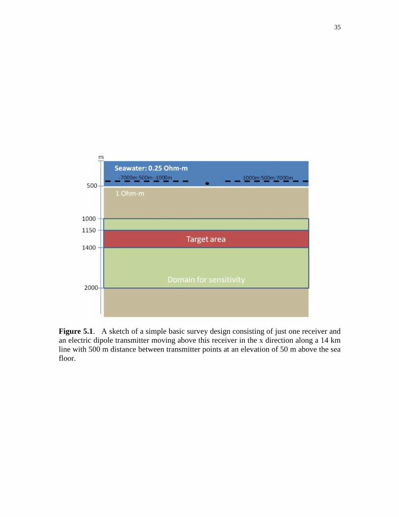
transmitter towed at some elevation above the sea bottom. We consider a simple basic
survey, consisting of just one receiver and an electric dipole transmitter moving above
this receiver in the x direction along a 14 km line at an elevation of 50 m above the sea
bottom (Figure 5.1). The transmitter generates a frequency domain EM field with a
frequency of 0.1 Hz from the points located every 500 m along the transmitter line. Later,
we will use different frequencies for analysis of the controlled sensitivity. The maximum
and minimum transmitter-receiver offsets are 7 km and 1 km, respectively. A single
receiver is located at the sea floor and measures the Ex component of the electric field
and the Hy component of the magnetic field. The background geoelectric model consists
of a seawater layer with a thickness of 500 m, a resistivity of 0.25 Ohm-m, and a layer of

29
conductive sea bottom sediments with a resistivity of 1 Ohm-m. The domain for our
sensitivity study extends from 1000 m to 2000 m in depth
5.2 1D integrated sensitivities of
the basic MCSEM survey
In order to understand the concepts of the integrated sensitivity and the weighted
integrated sensitivity, we compute these sensitivities for the basic survey design
described in Figure 5.1. Figures 5.2 and 5.3 present the plots of the original integrated
sensitivities for this basic survey (shown by the red dashed lines). We can see that the
integrated sensitivities for both electric and magnetic field components decrease rapidly
with the depth, indicating that the survey data are mostly sensitive to the upper layers of
the sea bottom formations. Those figures also present plots of the weighted integrated
sensitivities (shown by the blue dashed lines). Note that, in order to be able to compare
these two sensitivity distribution, we have plotted the sensitivities normalized by their
maximum value. One can see that the application of the data weights increases the
integrated sensitivity of the survey significantly. That is why data weighting is important
in MCSEM data interpretation.
5.3 Selection of the 1D a priori sensitivity
As we discussed in Chapter 4, we select a priori sensitivity P based on the
estimated depth of the reservoir. Theoretically, we can select any form for an a priori
sensitivity, but practically, we have to select a physically realizable form; otherwise it

30
would be computationally difficult to find a desired controlled sensitivity that would
satisfy equation (4.1).
For the 1D controlled sensitivity, we will consider three types of a priori
sensitivities. First, in Model 1 we simply construct the a priori sensitivity using the
maximum and minimum values of the original integrated sensitivity for both the x
component of the electric field, Ex, and for the y component of the magnetic field, Hy.
We set the maximum value for the a priori sensitivity within the target area ranging from
1150 m to 1400 m, and assign the minimum value for the sensitivity to other depths for
both electric and magnetic fields (Figure 5.4). We construct the a priori sensitivity of
Model 1 for the magnetic field component, Hy, in the same way as for the electric field
component, Ex.
In Model 2, we keep the same target area, but increase the minimum value of the
a priori sensitivity of Model 1.
Lastly, in Model 3 we use the same maximum and minimum values of the a priori
sensitivity as in Model 2, but locate the target area at a depth ranging from 1450 m to
1800 m. Note that, in graphical representations of the a priori and controlled sensitivities,
we plot the corresponding values normalized by the maximum of the original sensitivity.
5.4 Determining 1D controlled sensitivity
by inversion
We have applied an inversion method, described in section 4.2, in order to find
the controlled sensitivity according to equation (4.1). We will analyze the results using
three different types of models. All of these models are based on the simple basic survey

31
design, presented in Figure 5.1. The difference among the models is the manner in which
the a prior sensitivity is selected. We also consider the controlled sensitivities computed
for the Ex or Hy components, and for different frequencies.
5.4.1 1D controlled sensitivity for Model 1
As mentioned in the previous section, we use the maximum and the minimum
values of the original sensitivity to design the a priori sensitivity for Model 1. The target
area is located in the depth interval ranging from 1150 m to 1400 m.
Figure 5.4 shows an inversion result for the controlled sensitivity of the Ex
component, at a frequency of 0.1 Hz. From this figure, we can see that the original
sensitivity (red dashed line) decreases rapidly with the depth. After applying the data
weighting kernel matrix Q, which is determined from solving the minimization problem
(4.10), and calculating the corresponding controlled sensitivity using equation (4.11), we
can see that the obtained controlled sensitivity (black dashed line) corresponds well to the
a priori preselected sensitivity (solid line), increasing the sensitivity in the target area.
The sensitivity plots for the magnetic component have similar behavior, as can be seen in
Figure 5.5.
5.4.2 1D controlled sensitivity for Model 2
In Model 2, we have slightly modified the a priori sensitivity by using half the
maximum of the original integrated sensitivity in the depth intervals outside the target
area. Figure 5.6 shows the plots of the a priori, original, and controlled integrated
sensitivities normalized by the maximum of the original sensitivity. The sensitivities are

32
computed for the electric field component, Ex, at a frequency of 0.1 Hz. One can see a
very good representation by the controlled sensitivity of the designed a priori resistivity.
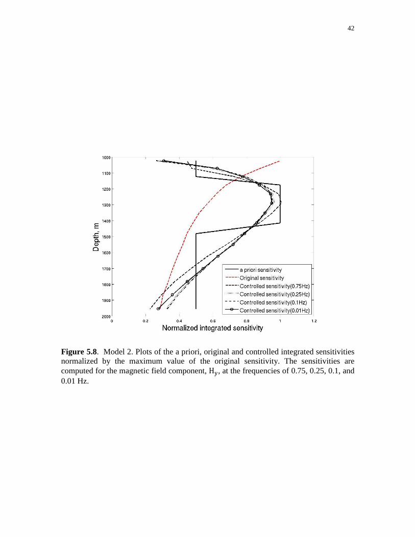
In the next set of numerical experiments, we calculate the corresponding
controlled sensitivities for cases of both the E� and H� components for a number of
decreasing frequencies, from 0.75 Hz to 0.01 Hz (Figures 5.7 and 5.8), in order to
analyze controlled sensitivity distributions computed with different frequencies. From
there results, we can see that the obtained controlled sensitivity curves represent well the
a priori selected sensitivity, providing the maximum sensitivity within the target area.
Also, we can see that the curve with a higher frequency increases more within the target
area and decreases outside of the target area. Therefore, higher frequency more
effectively controls the sensitivity, if the target area is located within a relatively shallow
depth interval. Note that, for every frequency, the linear system of equations (4.28) was
iteratively solved for a 1% level of misfit, as shown in Figure 5.9.
We can also calculate the controlled sensitivity for multifrequency data. Figure
5.10 presents a plot of the controlled sensitivity calculated for two frequencies of 0.25 Hz
and 0.1 Hz for the electric, Ex, and magnetic, Hy, components, respectively. One can see
that the result is improved, when we use multifrequency data in comparison with single-
frequency controlled sensitivity.
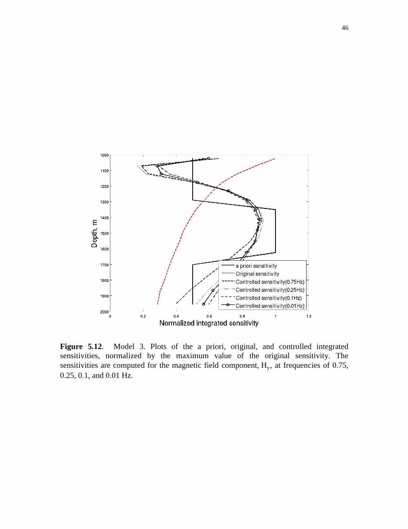
5.4.3 1D controlled sensitivity for Model 3
Finally, we consider Model 3 with the target area located at a depth ranging from
1450 m to 1800 m, and calculate the corresponding controlled sensitivity for the Ex and
Hy components, using different frequencies ranging from 0.75 to 0.01 Hz.

33
Figure 5.11 shows the controlled sensitivities of the Ex components for the
frequencies 0.75, 0.25, 0.1 and 0.01 Hz. One can see that the peak points of the obtained
sensitivity curves are getting closer to those of the target area, as the frequency gets lower.
The skin depth of an electromagnetic field with the higher frequency is larger than for a
lower frequency. Physically, it is easier to control the sensitivity by using the lower
frequency if the target area is located at a relatively deeper depth interval. We calculate
the controlled sensitivity for the Hy component with a number of decreased frequencies
from 0.75 Hz to 0.01 Hz (Figure 5.12).
Finally, we present in Figure 5.13 the plots of the controlled sensitivity calculated
for Model 3 using two frequencies of 0.25 Hz and 0.1 Hz for the electric, Ex , and
magnetic, Hy, components, respectively. One can see that the result is improved over
those obtained for a singular frequency.
5.4.4 Characteristics of the data weighting kernel matrix Q
The maps of the corresponding matrices Q for Model 2, computed for the electric
field component, Ex, at the frequencies of 0.75, 0.25, 0.1, and 0.01 Hz, are shown in
Figures 5.14, 5.15, 5.16 and 5.17, respectively. One can clearly see the symmetric
structure of matrix Q in these images. Also, we observe an oscillating "radiating" pattern
of matrix Q composed of the real positive and negative values. This pattern indicates that
the application of this matrix to the observed data may result in the artificial interference
of the fields produced by the transmitters in different locations, computed according to
formula (4.5). The matrix changes the magnitude and the phase of the EM signal, unlike

34
the diagonal matrix of data weights no that changes only their magnitude. This property
of matrix Q will be discussed in section 6.4.5 as well.
35
Figure 5.1. A sketch of a simple basic survey design consisting of just one receiver and an electric dipole transmitter moving above this receiver in the x direction along a 14 km line with 500 m distance between transmitter points at an elevation of 50 m above the sea floor.

36
Figure 5.2. Plots of the original and weighted integrated sensitivities normalized by the corresponding maximum values. The sensitivities are computed for the electric field component, E�, at a frequency of 0.1 Hz.

37
Figure 5.3. Plots of the original and weighted integrated sensitivities normalized by the corresponding maximum values. The sensitivities are computed for the magnetic field component, H�, at a frequency of 0.1 Hz.

38
Figure 5.4. Model 1. Plots of the original and a priori sensitivities normalized by the maximum value of the original sensitivity. The sensitivities are computed for the electric field component, E�, at a frequency of 0.1 Hz.

39
Figure 5.5. Model 1. Plots of the a priori, original, and controlled integrated sensitivities, normalized by the maximum value of the original sensitivity. The sensitivities are computed for the electric field component, Ex, at a frequency of 0.1 Hz.

40
Figure 5.6. Model 2. Plots of the a priori, original, and controlled integrated sensitivities, normalized by the maximum value of the original sensitivity. The sensitivities are computed for the electric field component, Ex, at a frequency of 0.1 Hz.

41
Figure 5.7. Model 2. Plots of the a priori, original, and controlled integrated sensitivities normalized by the maximum value of the original sensitivity. The sensitivities are computed for the electric field component, E�, at the frequencies of 0.75, 0.25, 0.1, and 0.01 Hz.
42
Figure 5.8. Model 2. Plots of the a priori, original and controlled integrated sensitivities normalized by the maximum value of the original sensitivity. The sensitivities are computed for the magnetic field component, H�, at the frequencies of 0.75, 0.25, 0.1, and 0.01 Hz.

43
Figure 5.9. Plots of the misfit and parametric functionals versus iteration number in the inversion for the controlled integrated sensitivity for Ex component at a frequency of 0.1 Hz.

44
Figure 5.10. Model 2. Plots of the a priori, original and controlled integrated sensitivities normalized by the maximum value of the original sensitivity. The sensitivities are computed for two frequencies of 0.25 and 0.1 Hz for the electric, E�, and magnetic, H�, components, respectively.

45
Figure 5.11. Model 3. Plots of the a priori, original, and controlled integrated sensitivities, normalized by the maximum value of the original sensitivity. The sensitivities are computed for the electric field component, E�, at frequencies of 0.75, 0.25, 0.1, and 0.01 Hz.
46
Figure 5.12. Model 3. Plots of the a priori, original, and controlled integrated sensitivities, normalized by the maximum value of the original sensitivity. The sensitivities are computed for the magnetic field component, Hy, at frequencies of 0.75, 0.25, 0.1, and 0.01 Hz.

47
Figure 5.13. Model 3. Plots of the a priori, original, and controlled integrated sensitivities, normalized by the maximum value of the original sensitivity. The sensitivities are computed for two frequencies of 0.25 and 0.1 Hz for the electric, E�, and magnetic, H�, components, respectively.

Figure 5.14. A map of matrix Q for Model 2, computed for electric field component,at a frequency of 0.75 Hz.
A map of matrix Q for Model 2, computed for electric field component,
48
A map of matrix Q for Model 2, computed for electric field component, ,

Figure 5.15. A map of matrix Q for Model 2, computed for electric field component, at a frequency of 0.25 Hz.
. A map of matrix Q for Model 2, computed for electric field component,
49
. A map of matrix Q for Model 2, computed for electric field component, ,

Figure 5.16. A map of matrix Q for Model 2, computed for electric field component, at a frequency of 0.1 Hz.
. A map of matrix Q for Model 2, computed for electric field component,
50
. A map of matrix Q for Model 2, computed for electric field component, ,

Figure 5.17. A map of matrix Q for Model 2, computed for electric field component, at a frequency of 0.01 Hz.
. A map of matrix Q for Model 2, computed for electric field component,
51
. A map of matrix Q for Model 2, computed for electric field component, ,

CHAPTER 6
NUMERICAL STUDY OF 2D CONTROLLED
SENSITIVITY
6.1 Survey design for 2D controlled sensitivity
In the previous chapter, we have shown the application of the developed method
for computing 1D controlled sensitivity. In this chapter, we extend the method to
compute 2D controlled sensitivity. We still consider a simple basic MCSEM survey
design similar to one shown in Figure 5.1. However we consider the survey with not only
one receiver, but also with three receivers, as shown in Figure 6.1. Those receivers are
located at the sea floor and measure the E� component of the electric field and the H�
component of the magnetic field. An electric dipole transmitter is moving above the
receivers in the x direction along a 14 km line at an elevation of 50 m above the sea
bottom. The transmitter generates a frequency domain EM field with a frequency of 0.1
Hz from the points located every 500 m along the transmitter line. We will also use
different frequencies in order to analyze the effect of the frequency on the controlled
sensitivity. The maximum and minimum transmitter-receiver offsets are 7 km and 1 km,
respectively. The background geoelectric model consists of a seawater layer with a
thickness of 500 m, and a resistivity of 0.25 Ohm-m, and a layer of conductive sea

53
bottom sediments with a resistivity of 1 Ohm-m. The domain of the sensitivity study
extends from 1000 m to 2000 m in depth.
6.2 2D integrated sensitivities for the basic
MCSEM survey
Using a simple basic survey design presented in Figure 6.1, we compute the
original and the weighted integrated sensitivities for the Ex component of the electric
field and the Hy component of the magnetic field.
Figure 6.2 presents the plots of the original integrated sensitivity (the top panel)
and the weighted integrated sensitivity (the bottom panel) for the basic survey design
with only one receiver, computed for the Ex component, and at a frequency of 0.1 Hz.
Both sensitivities are normalized to their maximum values.
Without data weighting, the original integrated sensitivity decreases rapidly with
the depth, indicating that the survey data are mostly sensitive to the conductivity in the
vicinity of the receiver location only, as one can see in the top panel of Figure 6.2. With
data weighting, one can see from the bottom panel in Figure 6.2 that the integrated
sensitivity increases in a large area away from the receiver. Figure 6.3 presents the
sensitivity distributions computed for a survey with three receivers for the Ex component
and a frequency of 0.1 Hz.
In this case, the survey data are more sensitive to the conductivity variations than
for one receiver only. From these experiments, we conclude that using more receivers
makes it easier for us to control the sensitivity because the data obtained from multiple

54
receivers are more sensitive to the sea bottom conductivity. The sensitivity plots for the
magnetic component have similar behavior, as one can see in Figures 6.2 and 6.3.
6.3 Selection of the a priori sensitivity
In the case of 2D controlled sensitivity, we construct four types of models for a
priori sensitivities for both the x component of the electric field, E� and the y component
of the magnetic field, H�:
1) Model 1 - horizontally extended target area in the shallow layer of the sea
bottom formation.
2) Model 2 - vertically extended target area.
3) Model 3 - box shaped target area.
4) Model 4 - horizontally extended target area in the deep layer of the sea bottom
formation.
We set the maximum value of the original sensitivity within the target area, and
assign the minimum value of the sensitivity to surrounding areas for both electric and
magnetic fields.
6.4 Determining 2D controlled sensitivity by inversion
In this section we present the results of computing the 2D controlled sensitivity
for four models. In each model, we consider the effects of the frequencies, and the
number of receivers.

55
6.4.1 2D controlled sensitivity for Model 1
In the case of Model 1, we construct a simple a priori sensitivity, whose target
area is extended horizontally at a relatively shallow depth interval ranging from 1200 m
to 1400 m. We present only one example of a priori sensitivity computed for the Ex
component at a frequency of 0.1 Hz (Figure 6.4).
Figure 6.5 shows the 2D controlled sensitivity computed for the survey with one
receiver, measuring the Ex component, at a frequency of 0.1 Hz. The white outline box in
this figure indicates the location of the target area. Comparing this result with the original
sensitivity distribution, presented in Figure 6.2, one can see that the part with high
sensitivity is moved from the vicinity of the receiver location to within the target area.
This result proves that the sensitivity can be controlled by applying the data weighting
kernel matrix Q to the survey data, focusing the sensitivity with respect to the target area.
In the next example, we compute the controlled sensitivity with the same
parameters as above, but changing the frequency from 0.1 Hz to 0.01 Hz (Figure 6.6).
One can see that the obtained controlled sensitivity distribution represents well the a
priori sensitivity, increasing the sensitivity within the target area.
In addition, the sensitivity becomes broader and deeper, but the maximum
sensitivity decreases in comparison with 0.1 Hz (Figure 6.6). This phenomenon is related
to the skin depth effect, as explained above.
We can also calculate the controlled sensitivity for multiple receivers. Figures 6.7
and 6.8 present the plots of controlled sensitivity computed for three receivers at a
frequency of 0.1 Hz for the electric, Ex, and the magnetic, Hy, components, respectively.
We can see that the results are improved over those obtained for one receiver. Note that

56
the sensitivity distributions are normalized by the maximum of the corresponding a priori
sensitivities.
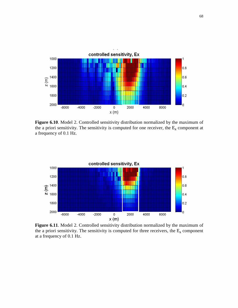
6.4.2 2D controlled sensitivity for Model 2
In the case of Model 2, a priori sensitivity has a vertical target area ranging from
1000 m to 3000 m in the x direction as shown in Figure 6.9.
Figures 6.10 and 6.11 present the controlled sensitivity distributions computed for
the Ex component, at a frequency of 0.1 Hz, and for one receiver and three receivers,
respectively. Both figures show very good results increasing the sensitivities within the
target area. One can also see that the result is improved, when we use three receivers
instead of only one, as they controlled sensitivity focused more on the target area. We
also calculate the controlled sensitivity for the Hy component, three receivers, and a
frequency of 0.1 Hz as shown in Figure 6.12. One can see that the controlled sensitivity
increases in the target area as well.
6.4.3 2D controlled sensitivity for Model 3
We now construct a priori sensitivity with the box shaped target area, ranging
from 1000 m to 2000 m in the x direction and from 1200 m to 1400 m in the depth
(Figure 6.13). This target area is produced by an overlap between the target areas of
Model 1 and Model 2. Figures 6.14 and 6.15 present the controlled sensitivities obtained
for the E�and the H� components, respectively. The sensitivities are computed for three
receivers at a frequency of 0.1 Hz. Both figures also show good results, placing the
maximum values of the sensitivities within the target areas.

57
6.4.4 2D controlled sensitivity for Model 4
In the case of final Models, we locate the target area horizontally in the deeper
layer than one of Model 1, ranging from 1500 m to 1700 m in the depth as shown in
Figure 6.16.
We compute the controlled sensitivity for the Ex component, three receivers, at
the frequencies of 0.1 and 0.01 Hz, as shown in Figures 6.17 and 6.18, respectively. As
we have expected from the study with a similar situation of the 1D controlled sensitivity
in section 5.4.3, both sensitivity distributions show improved results in comparison with
the original sensitivity. When we compare those two results, we can see that the
sensitivity with lower frequency is broader and deeper than that with higher frequency.
Also we can see that as the frequency decreases, the maximum of the obtained sensitivity
shifts down towards the target area.
6.4.5 Characteristics of the data weighting kernel matrix Q
In section 5.4.4, we have analysed the data weighting kernel matrix Q for 1D
controlled sensitivity. In this section, we will illustrate matrix Q for 2D controlled
sensitivity based on the survey with three receivers. If the survey has multiple
transmitters and receivers, matrix Q becomes more complicated increasing in size
proportional to the number of data. To understand better how matrix Q affects the data, it
would be necessary to analyze not only matrix Q but also the weighted data Im as well.
Figures 6.20 through 6.23 present the maps of matrices Q computed for different
a priori sensitivities for Model 1 through Model 4, respectively. All maps are plotted for
the Ex component at a frequency of 0.1 Hz, and a survey with 3 receivers and 26

58
transmitter points as shown in Figure 6.1. As the number of data is now 78, the vector of
the observed data can be represented as
I � �'M, … , 'Fä, 'F�, … , 'åF, … , '�æ�Í,
Note that the data are arranged in the order of receiver and then transmitter based on the
reciprocity principle. So, the first 26 components indicate the data obtained from the first
receiver and the all sets of transmitter, and so on. For convenience, we number the
receivers in the increasing order in the x direction shown in Figure 6.1. According to the
matrix notation of the matrix Q in equation (4.29), the application of the matrix Q to data
generates the weighted data:
ImVç � �'mVçM, … , 'mVçFä, 'mVçF�, … , 'mVçåF, … , 'mVç�æ�Í,
where the components of the weighted data ('mVç�) are
'mVç� � U ¼�»'»�æ
»²M , � � 1,2, … ,78. One can see that the weighted data are superposed by all set of the transmitter as well as
the receivers.
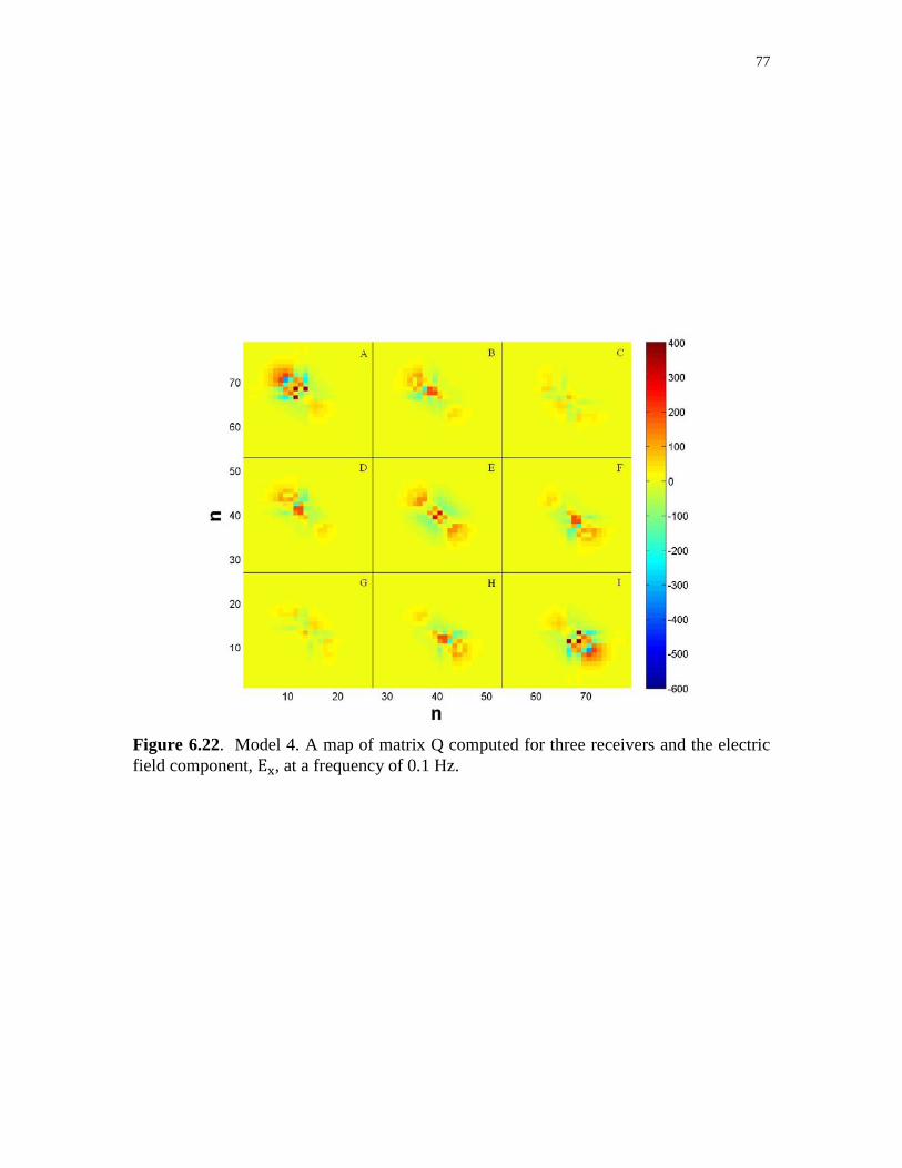
Each matrix Q in Figures 6.19 through 6.22 can be divided into 9 small sections
with a size of 26 × 26 depending on the number of receivers, and we call them section A
~ I, as denoted in Figure 6.19. One can see that each section also shows the radiating and
oscillating pattern as shown in the maps of the 1D case. Also, when we apply matrix Q to
the data, we can see that a set of the data related to one receiver is affected by only one

59
column set of the sections of the matrix Q. For example, the data set from the first
receiver �'M, … , 'Fä�Í is multiplied by sections A, D and G only.
Let us compare the maps of matrices Q for Model 1 and 4, which are computed
for shallow and deep horizontal target areas, respectively (Figures 6.19 and 6.22). First,
those matrices are symmetric about their centers, which are called centrosymmetric
matrices. Those results are in agreement with the fact that the corresponding survey
geometries, including locations of transmitters, receivers and target area, are designed
symmetrically along the vertical line with the receiver in the center. Also, both matrices
are more weighted in the diagonal sections, which means they are more focused on the
data set related to the one receiver. For example, matrix Q gives more weights to the data
observed by the first receiver, in order to generate the corresponded weighted data with
the same receiver set. The difference between Figures 6.19 and 6.22 is that the matrix Q
for Model 1 is more weighted and focused in the center of each section than that for
Model 4. We can also conclude that the matrix Q emphasizes the data with short
transmitter - receiver offsets in the case of the sensitivity focused on the shallow area.
This behavior agrees well with the fact that the depth of low frequency (almost DC
current) propagation is proportional to the transmitter – receiver offset.
Similar behavior is observed in Figures 6.20 and 6.21, which are computed for the
target areas located on the right side of the receivers. First, matrices provide more
weights in the right side and in the bottom of the area of investigation. Also, one can see
that the sensitivity for Model 2 (Figure 6.12) is more focused in the subsurface in
comparison to those for Model 3 (Figure 6.15). This difference makes matrix Q for
Model 2 more weighted and focused in the center of the corresponding section.

60
Figure 6.23 presents an example of the application of matrix Q (Figure 6.20) to
the observed data. The top panel shows the magnitude of the E� component of the electric
field observed in the center receiver. The bottom panel presents the weighted data,
ImVm � ©I. One can see that, after applying matrix Q to data d, the observed signal is
shifted toward the target area, which is located from 1000 m to 3000 m in the x direction.

Figure 6.1. A sketch of a simple basic survey design consisting of three receivers and an electric dipole transmitter moving above this receiver in the x direction along a 14 km line with 500 m distance between transmitter points at an elevation of 50 m above the floor.
. A sketch of a simple basic survey design consisting of three receivers and an electric dipole transmitter moving above this receiver in the x direction along a 14 km line with 500 m distance between transmitter points at an elevation of 50 m above the
61
. A sketch of a simple basic survey design consisting of three receivers and
an electric dipole transmitter moving above this receiver in the x direction along a 14 km line with 500 m distance between transmitter points at an elevation of 50 m above the sea

62
Figure 6.2. Original and weighted integrated sensitivity distributions for the basic survey consisting of one receiver, which measures the E� component of the electric field. Both sensitivities are normalized by the corresponding maximum value. The sensitivities are computed for the E� component, at a frequency of 0.1 Hz.

63
Figure 6.3. Original and weighted integrated sensitivity distributions for the basic survey consisting of three receivers, which measure the E� component of the electric field. Both sensitivities are normalized by the corresponding maximum value. The sensitivities are computed for the E� component, at a frequency of 0.1 Hz.

64
Figure 6.4. Model 1. A priori sensitivity distribution normalized by the maximum of the a priori sensitivity. The sensitivity is computed for the Ex component at a frequency of 0.1 Hz.

65
Figure 6.5. Model 1. Controlled sensitivity distribution normalized by the maximum of the a priori sensitivity. The sensitivity is computed for one receiver only, the E� component at a frequency of 0.1 Hz.
Figure 6.6. Model 1. Controlled sensitivity distribution normalized by the maximum of the a priori sensitivity. The sensitivity is computed for one receiver only, the E� component at a frequency of 0.01 Hz.

66
Figure 6.7. Model 1. Controlled sensitivity distribution normalized by the maximum of the a priori sensitivity. The sensitivity is computed for three receivers, the Ex component at a frequency of 0.1 Hz.
Figure 6.8. Model 1. Controlled sensitivity distribution normalized by the maximum of the a priori sensitivity. The sensitivity is computed for three receivers, the H� component at a frequency of 0.1 Hz.

67
Figure 6.9. Model 2. A priori sensitivity distribution normalized by the maximum of the a priori sensitivity. The sensitivity is computed for the Ex component at a frequency of 0.1 Hz.
68
Figure 6.10. Model 2. Controlled sensitivity distribution normalized by the maximum of the a priori sensitivity. The sensitivity is computed for one receiver, the E� component at a frequency of 0.1 Hz.
Figure 6.11. Model 2. Controlled sensitivity distribution normalized by the maximum of the a priori sensitivity. The sensitivity is computed for three receivers, the E� component at a frequency of 0.1 Hz.

69
Figure 6.12. Model 2. Controlled sensitivity distribution normalized by the maximum of the a priori sensitivity. The sensitivity is computed for three receivers, the H� component at a frequency of 0.1 Hz.

70
Figure 6.13. Model 3. A priori sensitivity distribution normalized by the maximum of the a priori sensitivity. The sensitivity is computed for the Ex component at a frequency of 0.1 Hz.

71
Figure 6.14. Model 3. Controlled sensitivity distribution normalized by the maximum of the a priori sensitivity. The sensitivity is computed for three receivers, the E� component at a frequency of 0.1 Hz.
Figure 6.15. Model 3. Controlled sensitivity distribution normalized by the maximum of the a priori sensitivity. The sensitivity is computed for three receivers, the H� component at a frequency of 0.1 Hz.

72
Figure 6.16. Model 2. A priori sensitivity distribution normalized by the maximum of the a priori sensitivity. The sensitivity is computed for the E� component at a frequency of 0.1 Hz.

73
Figure 6.17. Model 4. Controlled sensitivity distribution normalized by the maximum of the a priori sensitivity. The sensitivity is computed for three receivers, the E� component at a frequency of 0.1 Hz.
Figure 6.18. Model 4. Controlled sensitivity distribution normalized by the maximum of the a priori sensitivity. The sensitivity is computed for three receivers, the E� component at a frequency of 0.01 Hz.

74
Figure 6.19. Model 1. A map of matrix Q computed for three receivers and the electric field component, E�, at a frequency of 0.1 Hz.

75
Figure 6.20. Model 2. A map of matrix Q computed for three receivers and the electric field component, E�, at a frequency of 0.1 Hz.

76
Figure 6.21. Model 3. A map of matrix Q computed for three receivers and the electric field component, E�, at a frequency of 0.1 Hz.
77
Figure 6.22. Model 4. A map of matrix Q computed for three receivers and the electric field component, E�, at a frequency of 0.1 Hz.

78
Figure 6.23. Model 2. Application of the data kernel matrix Q to the observed data d (top panel) based on the basic MCSEM survey design with three receivers. The data are computed for the E� component at a frequency of 0.1 Hz. The weighted data (bottom panel) present the result of application of matrix Q to original data d.

CHAPTER 7
CONCLUSIONS
In this thesis, I discuss the methods of the original and weighted integrated
sensitivity calculations. Those methods make it possible to evaluate a cumulative
response of the observed EM data to the conductivity perturbations for a survey with a
multiple transmitter/receiver observation system.
From numerical experiments for 1D and 2D original and weighted integrated
sensitivities based on a simple basic MCSEM survey, I have confirmed that the obtained
EM data are sensitive in the vicinity of the receiver location only and the sensitivity
decreases rapidly with depth. Moreover, I demonstrate that the application of the data
weighting to the data can increase the sensitivity significantly even in the far zone from
the receiver location.
Based on the integrated sensitivity method, I have formulated a concept of
controlled sensitivity, which enables the sensitivity of the MCSEM survey to be focused
on a specific area of the sea bottom formations, where a potential target may be located.
This approach is based on the optimization of the integrated sensitivity of the MCSEM
survey. I have also considered a numerical method for determining the data weighting
kernel matrix, which focuses the integrated sensitivity within the target area, using a

80
linear inversion algorithm, which is based on the regularized conjugate-gradient (RCG)
method.
I have demonstrated this concept with numerical studies of the 1D and 2D
controlled sensitivities of the MCSEM survey. In both cases, the method successfully
controls the integrated sensitivity distributions for both the E� component of the electric
field and the H� component of the magnetic field, increasing the sensitivities within
different types of the a priori selected target areas.
In these numerical studies, I have examined the effects of the survey parameters
on the controlled sensitivity results. First, I have found that the frequency of a transmitted
EM signal affects the controlled sensitivity result, agreeing with the skin depth effect of
the EM field. When I compute the controlled sensitivity at a higher frequency, the
maximum of the sensitivity increases more in the target area. I have also found that the
application of controlled sensitivity method to the multifrequency data provides more
focused sensitivity than for singular frequency. Second, I have also examined the
controlled sensitivity for the survey data with a different number of receivers. We can
observe that the data with a larger number of receivers show a better result for controlled
sensitivity plot than those with only one receiver, being more focused within the target
area.
In the 1D controlled sensitivity study, I have found that the data weighting kernel
matrix Q has an oscillating “radiating” pattern, which indicates that the application of this
matrix to the observed data may result in the predicted type of interference of the fields
produced by the transmitters in different locations. This pattern has also shown in the 2D
controlled sensitivity, when we divide the matrix into small sections depending on the

81
survey information. We could see that the matrix Q controls the data, steering the data
toward the target area. Thus, physically, the developed method can be described as a
controlled interference of the EM fields, generated by a set of transmitters and receivers.
In this sense the developed method uses physical principles similar to the synthetic
aperture radar method. The main difference is that the controlled sensitivity approach is
based on a rigorous optimization technique.
This method allows us to find the optimal parameters of the data weighting in
order to increase the resolution of the MCSEM data within an a priori selected target area,
such as the prospective location of HC reservoirs.

REFERENCES
Carazzone, J. J., O. M. Burtz, K.E. Green, and D. A. Pavlov, 2005, Three dimensional imaging of marine CSEM data: 75th Annual International Meeting, SEG, Expanded Abstract, 575-578.
Constable, S., and L. J. Srnka, 2007, An introduction to marine controlled-source electromagnetic methods for hydrocarbon exploration, Geophysics, 72, WA3-WA12.
Cox, C. S., 1981, On the electrical conductivity of the oceanic lithosphere, Physics of the Earth and Planetary Interiors, 25, 196–201.
Dubrovskiy, V. G., and N. V. Kondratieva, 1976, Basic results of the magnetotelluric soundings in the Turkmen sector of the Caspian Sea: Izvestia AN SSSR, Physics of the Earth, 3, 67-76.
Edwards, N, 2005, Marine controlled source electromagnetics: principles, methodologies, future commercial applications, Geophysics, 26, 675-700.
Edward, R. N., Nobes, D. C. and Gomez-Trevino, E. 1984, Offshore electrical exploration of sedimentary basins: the effects of anisotropy in horizontally isotropic, layered media, Geophysics, 49, 566-576.
Eidesmo, T., S. Ellingsrud, L. M. MacGregor, S. Constable, M. C. Sinha, S. Johansen, F. N. Kong, and H. Westerdahl, 2002, Sea Bed Logging (SBL), a new method for remote and direct identification of hydrocarbon filled layers in deepwater areas: First Break, 20, 144-152.
Fan, Y., R. Snieder, E. Slob, J. Hunziker, J. Singer, J. Sheiman, and M. Rosenquist, 2010, Synthetic aperture controlled source electromagnetics, Geophysical Research Letters, 37, L13305, doi: 10.1029/2010GL043981.
Gribenko, A., and M. S. Zhdanov, 2007, Rigorous three-dimensional inversion of marine CSEM data based on the integral equation method, Geophysics, 72, WA73-WA84
Hohmann, G. W., 1975, Three-dimensional induced polarization and electromagnetic modeling, Geophysics, 40, 309-324.
Jupp, D. L. B. and Vozoff, K., 1976, Two-dimensional magnetotelluric inversion, Geophys. J. R. astr. Soc., 50, 333-352.

83
Kaputerko, A., and M. S. Zhdanov, 2010, Analysis of integrated sensitivity of CSEM data in offshore hydrocarbon exploration, Proceedings of Annual Meeting of the Consortium for Electromagnetic Modeling and Inversion, 127-162.
MacGregor L. M., and M. Sinha, 2000, Use of marine controlled-source electromagnetic sounding for sub-basalt exploration, Geophysical Prospecting, 48, 1091-1106.
McGillivray, P. R., D. W. Oldenburg, R. G. Ellis, and T. M. Habashy, 1994, Calculation of sensitivities for the frequency-domain electromagnetic problem, Geophysical Journal International, 116, 1-4.
McGillivray, P. R., and D. W. Oldenburg, 1990, Methods for calculating Frechet derivatives and sensitivities for the nonlinear inverse problem: a comparative study, Geophysical Prospecting, 38, 499-524.
Morten, J. P., A. K. Bjørke, and T. Støren, 2009, CSEM data uncertainty analysis for 3D inversion: 79th Annual international meeting, SEG, Expanded Abstracts, 28, 724.
Novysh, V. V., and G. A. Fonarev, 1966, The results of the electromagnetic study in the Arctic Ocean, Geomagnetism and Aeronomy, 6, 406-409.
Raiche, A. P., 1974, An integral equation approach to three-dimensional modeling, Geophysical Journal of the Royal Astronomical Society, 36, 363-376.
Rodi, W. L., 1976, A technique for improving the accuracy of finite element solutions for MT data, Geophys. J. R. astr. Soc., 44, 483-506.
Spiess, F. N., K. C. Macdonald, T. Atwater, R. Ballard, A. Carranza, D. Cordoba, C. Cox, V. M. Diaz Garcia, J. Francheteau, J. Guerrero, J. Hawkings, R. Haymon, R. Hessler, T. Juteau, M. Kastner, R. Larson, B. Luyendyk, J. D. Macdougall, S. Miller, W. Normark, J. Orcutt, and C. Rangin, 1980, East Pacific Rise: Hot spring sand geophysical experiments, Science, 207, 1421–1433.
Trofimov, I. L., and G. A. Fonarev, 1972, Some results of the magnetotelluric profilinf in the Arctic ocean: Izvestia AN SSSR, Physics of the Earth, (2), 81-92.
Weidelt, P., 1975a, Electromagnetic induction in three-dimensional structures, Jounal of Geophysics, 41 (1), 85-109.
Young, P. D., and C. S. Cox, 1981, Electromagnetic active source sounding near the East Pacific Rise, Geophysical Research Letters, 8, 1043–1046.
Zhdanov, M. S., 2002, Geophysical inverse theory and regularization problems, Elsevier.
Zhdanov, M. S., 2009, Geophysical electromagnetic theory and methods, Elsevier.
Zhdanov, M. S., 2010, Electromagnetic geophysics: Notes from the past and the road ahead, Geophysics, 75, 49-66.