controllability of nonlinear systems...controllability of nonlinear systems jean-michel coron...
TRANSCRIPT

Controllability of nonlinear systems
Jean-Michel Coron
Laboratory J.-L. Lions, University Pierre et Marie Curie (Paris 6)BCAM OPTPDE summer school, Bilbao, July 4-8 2011

The linear test
We consider the control system y = f(y, u) where the state is y ∈ Rn and
the control is u ∈ Rm. Let us assume that f(ye, ue) = 0. The linearized
control system at (ye, ue) is the linear control system y = Ay +Bu with
A :=∂f
∂y(ye, ue), B :=
∂f
∂u(ye, ue).(1)
If the linearized control system y = Ay +Bu is controllable, theny = f(y, u) is small-time locally controllable at (ye, ue).

Application to the baby stroller
Let us recall that the baby stroller control system is
y1 = u1 cos y3, y2 = u1 sin y3, y3 = u2, n = 3, m = 2.(1)
The linearized control system at (0, 0) ∈ R3 × R
2 is
y1 = u1, y2 = 0, y3 = u2,(2)
which is clearly not controllable. The linearized control system gives noinformation on the small-time local controllability at (0, 0) ∈ R
3 × R2 of
the baby stroller.
What to do if linearized control system is not controllable?
Question: What to do if
y =∂f
∂y(ye, ue)y +
∂f
∂u(ye, ue)u(1)
is not controllable?In finite dimension: One uses iterated Lie brackets.

Lie brackets and iterated Lie brackets
Definition (Lie brackets)
[X,Y ](y) := Y ′(y)X(y) −X ′(y)Y (y).(1)
Iterated Lie brackets: [X, [X,Y ]], [[Y,X], [X, [X,Y ]]] etc.Why Lie brackets are natural objects for controllability issues? Forsimplicity, from now on we assume that
f(y, u) = f0(y) +
m∑
i=1
uifi(y).
Drift: f0. Driftless control systems: f0 = 0.

Lie bracket for y = u1f1(y) + u2f2(y)
bca

Lie bracket for y = u1f1(y) + u2f2(y)
bca
(u1, u2) = (η1, 0)
y(ε)

Lie bracket for y = u1f1(y) + u2f2(y)
bca
(u1, u2) = (η1, 0)
y(ε)
(u1, u2) = (0, η2)
y(2ε)

Lie bracket for y = u1f1(y) + u2f2(y)
bca
(u1, u2) = (η1, 0)
y(ε)
(u1, u2) = (0, η2)
y(2ε)
(u1, u2) = (−η1, 0)
y(3ε)

Lie bracket for y = u1f1(y) + u2f2(y)
bca
(u1, u2) = (η1, 0)
y(ε)
(u1, u2) = (0, η2)
y(2ε)
(u1, u2) = (−η1, 0)
y(3ε)
bc
(u1, u2) = (0,−η2)
y(4ε)

Lie bracket for y = u1f1(y) + u2f2(y)
bca
(u1, u2) = (η1, 0)
y(ε)
(u1, u2) = (0, η2)
y(2ε)
(u1, u2) = (−η1, 0)
y(3ε)
bc
(u1, u2) = (0,−η2)
y(4ε) ≃ a+ η1η2ε2[f1, f2](a)
(ε → 0+)

Controllability of driftless control systems: Local
controllability
Theorem (P. Rashevski (1938), W.-L. Chow (1939))
Let O be a nonempty open subset of Rn and let ye ∈ O. Let us assumethat, for some f1, . . . , fm : O → R
n,
f(y, u) =
m∑
i=1
uifi(y), ∀(y, u) ∈ O × Rm.(1)
Let us also assume that
h(ye); h ∈ Lie f1, . . . , fm
= Rn.(2)
Then the control system y = f(y, u) is small-time locally controllable at(ye, 0) ∈ R
n × Rm.
The baby stroller system: Controllability
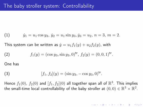
y1 = u1 cos y3, y2 = u1 sin y3, y3 = u2, n = 3, m = 2.(1)
This system can be written as y = u1f1(y) + u2f2(y), with
f1(y) = (cos y3, sin y3, 0)tr, f2(y) = (0, 0, 1)tr .(2)
One has
[f1, f2](y) = (sin y3,− cos y3, 0)tr.(3)
Hence f1(0), f2(0) and [f1, f2](0) all together span all of R3. This impliesthe small-time local controllability of the baby stroller at (0, 0) ∈ R
3 × R2.

Controllability of driftless control systems: Global
controllability
Theorem (P. Rashevski (1938), W.-L. Chow (1939))
Let O be a connected nonempty open subset of Rn. Let us assume that,for some f1, . . . , fm : O → R
n,
f(y, u) =
m∑
i=1
uifi(y), ∀(y, u) ∈ O × Rm.
Let us also assume that
h(y); h ∈ Lie f1, . . . , fm
= Rn, ∀y ∈ O.
Then, for every (y0, y1) ∈ O ×O and for every T > 0, there exists ubelonging to L∞((0, T );Rm) such that the solution of the Cauchy problemy = f(y, u(t)), y(0) = y0, satisfies y(t) ∈ O, ∀t ∈ [0, T ] and y(T ) = y1.

bc bc

bc bc

bc bcO

bc bcO
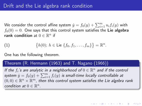
Drift and the Lie algebra rank condition
We consider the control affine system y = f0(y) +∑m
i=1 uifi(y) withf0(0) = 0. One says that this control system satisfies the Lie algebra
rank condition at 0 ∈ Rn if
h(0); h ∈ Lie f0, f1, . . . , fm
= Rn.(1)
One has the following theorem.
Theorem (R. Hermann (1963) and T. Nagano (1966))
If the fi’s are analytic in a neighborhood of 0 ∈ Rn and if the control
system y = f0(y) +∑m
i=1 fi(y) is small-time locally controllable at(0, 0) ∈ R
n × Rm, then this control system satisfies the Lie algebra rank
condition at 0 ∈ Rn.

Lie bracket for y = f0(y) + uf1(y), with f0(a) = 0
bca

Lie bracket for y = f0(y) + uf1(y), with f0(a) = 0
bca
u = −η
y(ε)

Lie bracket for y = f0(y) + uf1(y), with f0(a) = 0
bca
u = −η
y(ε)
bc
u = η
y(2ε)

Lie bracket for y = f0(y) + uf1(y), with f0(a) = 0
bca
u = −η
y(ε)
bc
u = η
y(2ε) ≃ a+ ηε2[f0, f1](a)ε → 0+
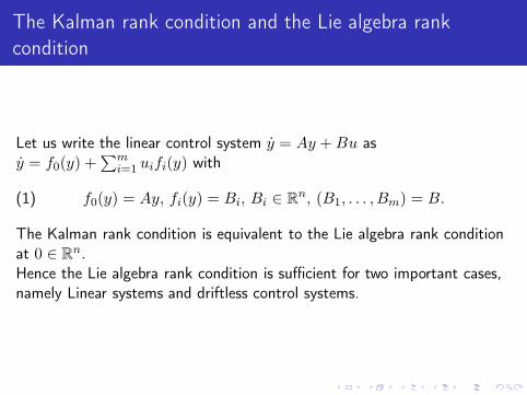
The Kalman rank condition and the Lie algebra rank
condition
Let us write the linear control system y = Ay +Bu asy = f0(y) +
∑mi=1 uifi(y) with
f0(y) = Ay, fi(y) = Bi, Bi ∈ Rn, (B1, . . . , Bm) = B.(1)
The Kalman rank condition is equivalent to the Lie algebra rank conditionat 0 ∈ R
n.Hence the Lie algebra rank condition is sufficient for two important cases,namely Linear systems and driftless control systems.

With a drift term: Not all the iterated Lie brackets are good
We take n = 2 and m = 1 and consider the control system
y1 = y22, y2 = u,(1)
where the state is y := (y1, y2)tr ∈ R
2 and the control is u ∈ R. Thiscontrol system can be written as y = f0(y) + uf1(y) with
f0(y) = (y22 , 0)tr, f1(y) = (0, 1)tr.(2)
One has [f1, [f1, f0]] = (2, 0)tr and therefore f1(0) and [f1, [f1, f0]](0) spanall of R2. However the control system (1) is clearly not small-time locallycontrollable at (0, 0) ∈ R
2 ×R.

References for sufficient or necessary conditions for
small-time local controllability when there is a drift term
A. Agrachev (1991),
A. Agrachev and R. Gamkrelidze (1993),
R. M. Bianchini and Stefani (1986),
H. Frankowska (1987),
M. Kawski (1990),
H. Sussmann (1983, 1987),
A. Tret’yak (1990).
...

Controllability of control systems modeled by linear PDE
There are lot of powerful tools to study the controllability of linear controlsystems in infinite dimension. The most popular ones are based on theduality between observability and controllability (related to the J.-L. LionsHilbert uniqueness method). This leads to try to prove observability
inequalities. There are many methods to prove this observabilityinequalities. For example:
Ingham’s inequalities and harmonic analysis: D. Russell (1967),
Multipliers method: Lop Fat Ho (1986), J.-L. Lions (1988),
Microlocal analysis: C. Bardos-G. Lebeau-J. Rauch (1992),
Carleman’s inequalities: A. Fursikov, O. Imanuvilov, G. Lebeau andL. Robbiano (1993-1996).
However there are still plenty of open problems.

The linear test
Of course when one wants to study the local controllability around anequilibrium of a control system in infinite dimension, the first step is toagain study the controllability of the linearized control system. If thislinearized control system is controllable, one can usually deduce the localcontrollability of the nonlinear control system. However this might besometimes difficult due to some loss of derivatives issues. One needs to usesuitable iterative schemes.
Remark
If the nonlinearity is not too big, one can get a global controllability result(E. Zuazua (1988), I. Lasiecka-R. Triggiani (1991) for semilinear waveequations, O. Imanuvilov (1995), A. Fursikov-O. Imanuvilov (1996), E.Fernández-Cara-E. Zuazua (2000) for semilinear heat equations).

The Euler control system
bc
x
y(t, x)
Ω
∂Ω
Γ0
Rn

Notations
Let ϕ : Ω → Rn, x = (x1, x2, . . . , xn) 7→ (ϕ1(x), ϕ2(x), . . . ϕn(x)), we
define div ϕ : Ω → R and (ϕ · ∇)ϕ : Ω → Rn by
div ϕ :=n∑
i=1
∂ϕi
∂xi,(1)
[(ϕ · ∇)ϕ]k =
n∑
i=1
ϕi∂ϕk
∂xi(2)
If n = 2, one defines curl ϕ : Ω → R by
curl ϕ :=∂y2∂x1
−∂y1∂x2
.(3)
Finally, for π : Ω → R, one defines ∇π : Ω → Rn by
∇π :=
(
∂π
∂x1,∂π
∂x2, . . . ,
∂π
∂xn
)
.(4)
Similarly notations if ϕ or π depends also on time t (one fixes the time...).

Controllability problem
We denote by ν : ∂Ω → Rn the outward unit normal vector field to Ω. Let
T > 0. Let y0, y1 : Ω → Rn be such that
div y0 = div y1 = 0, y0 · ν = y1 · ν = 0 on ∂Ω \ Γ0.(1)
Does there exist y : [0, T ]× Ω → Rn and p : [0, T ] × Ω → R such that
yt + (y · ∇)y +∇p = 0, div y = 0,(2)
y · ν = 0 on [0, T ]× (∂Ω \ Γ0),(3)
y(0, ·) = y0, y(T, ·) = y1?(4)
For the control, many choices are in fact possible. For example, for n = 2,one can take
1 y · ν on Γ0 with∫
Γ0y · ν = 0,
2 curl y at the points of [0, T ]× Γ0 where y · ν < 0.

A case without controllability
Γ1
Ω
∂Ω
Γ0
R2
Ω

Proof of the noncontrollability
Let us give it only for n = 2. Let γ0 be a Jordan curve in Ω. Let, fort ∈ [0, T ], γ(t) be the Jordan curve obtained, at time t ∈ [0, T ], from thepoints of the fluids which, at time 0, were on γ0. The Kelvin law tells usthat, if γ(t) does not intersect Γ0,
∫
γ(t)y(t, ·) ·
−→ds =
∫
γ0
y(0, ·) ·−→ds, ∀t ∈ [0, T ],(1)
We take γ0 := Γ1. Then γ(t) = Γ1 for every t ∈ [0, T ]. Hence, if
∫
Γ1
y1 ·−→ds 6=
∫
Γ1
y0 ·−→ds,(2)
one cannot steer the control system from y0 to y1.More generally, for every n ∈ 2, 3, if Γ0 does not intersect everyconnected component of the boundary ∂Ω of Ω, the Euler control system isnot controllable. This is the only obstruction to the controllability of theEuler control system.

Controllability of the Euler control system
Theorem (JMC for n = 2 (1996), O. Glass for n = 3 (2000))
Assume that Γ0 intersects every connected component of ∂Ω. Then theEuler control system is globally controllable in every time: For every T > 0,for every y0, y1 : Ω → R
n such that
div y0 = div y1 = 0, y0 · ν = y1 · ν = 0 on ∂Ω \ Γ0,(1)
there exist y : [0, T ]× Ω → Rn and p : [0, T ]× Ω → R such that
yt + (y · ∇)y +∇p = 0, div y = 0,(2)
y · ν = 0 on [0, T ]× (∂Ω \ Γ0)(3)
y(0, ·) = y0, y(T, ·) = y1.(4)

Comments on the proof
First try: One studies (as usual) the controllability of the linearized controlsystem around 0. This linearized control system is the control system
yt +∇p = 0, div y = 0, y · ν = 0 on [0, T ]× (∂Ω \ Γ0).(1)
For simplicity we assume that n = 2. Taking the curl of the first equation,on gets,
(curl y)t = 0.
Hence curl y remains constant along the trajectories of the linearizedcontrol system. Hence the linearized control system is not controllable.
Iterated Lie brackets and PDE control systems
Iterative Lie brackets have been used successfully for some control PDEsystems:
Euler and Navier Stokes control systems (different from the oneconsidered here): A. Agrachev and A. Sarychev (2005); A. Shirikyan(2006, 2007), H. Nersisyan (2010),
Schrödinger control system: T. Chambrion, P. Mason, M. Sigalottiand U. Boscain (2009).
However they do not seem to work here.

A problem with Lie brackets for PDE control systems
Consider the simplest PDE control system
yt + yx = 0, x ∈ [0, L], y(t, 0) = u(t).(1)
It is a control system where, at time t, the state is y(t, ·) : (0, L) → R andthe control is u(t) ∈ R. Formally it can be written in the formy = f0(y) + uf1(y). Here f0 is linear and f1 is constant.

Lie bracket for y = f0(y) + uf1(y), with f0(a) = 0
bca
u = −η
y(ε)
bc
u = η
y(2ε) ≃ a+ ηε2[f0, f1](a)ε → 0+
Problems of the Lie brackets for PDE control systems
(continued)
Let us consider, for ε > 0, the control defined on [0, 2ε] by
u(t) := −η for t ∈ (0, ε), u(t) := η for t ∈ (ε, 2ε).
Let y : (0, 2ε) × (0, L) → R be the solution of the Cauchy problem
yt + yx = 0, t ∈ (0, 2ε), x ∈ (0, L),(1)
y(t, 0) = u(t), t ∈ (0, 2ε), y(0, x) = 0, x ∈ (0, L).(2)
Then one readily gets, if 2ε 6 L,
y(2ε, x) = η, x ∈ (0, ε), y(2ε, x) = −η, x ∈ (ε, 2ε),(3)
y(2ε, x) = 0, x ∈ (2ε, L).(4)

Problems of the Lie brackets for PDE control systems
(continued)
∣
∣
∣
∣
y(2ε, ·) − y(0, ·)
ε2
∣
∣
∣
∣
L2(0,L)
→ +∞ as ε → 0+.(1)
For every φ ∈ H2(0, L), one gets after suitable computations
limε→0+
∫ L
0φ(x)
(
y(2ε, x) − y(0, x)
ε2
)
dx = −ηφ′(0).(2)
So, in some sense, we could say that [f0, f1] = δ′0. Unfortunately it is notclear how to use this derivative of a Dirac mass at 0.How to avoid the use of iterated Lie brackets?
The return method (JMC (1992))
y
t0
T

The return method (JMC (1992))
y
t0
T
y(t)

The return method (JMC (1992))
y
t0
T
y(t)
y0
y1
B0 B1

The return method (JMC (1992))
y
t0
T
y(t)
y(t)
y0
y1
B0 B1

The return method (JMC (1992))
y
t0
T
η
6 ε
y(t)
y(t)
y0
y1
B0 B1

The return method: An example in finite dimension
We go back to the baby stroller control system
y1 = u1 cos y3, y2 = u1 sin y3, y3 = u2.(1)
For every u : [0, T ] → R2 such that, for every t in [0, T ],
u(T − t) = −u(t), every solution y : [0, T ] → R3 of
˙y1 = u1 cos y3, ˙y2 = u1 sin y3, ˙y3 = u2,(2)
satisfies y(0) = y(T ). The linearized control system around (y, u) is
y1 = −u1y3 sin y3 + u1 cos y3, y2 = u1y3 cos y3 + u1 sin y3,y3 = u2,
(3)
which is controllable if (and only if) u 6≡ 0. We have got the controllabilityof the baby stroller system without using Lie brackets. We have only usedcontrollability results for linear control systems.

No loss with the return method
We consider the control system
Σ : y = f0(y) +m∑
i=1
uifi(y),
where the state is y ∈ Rn and the control is u ∈ R
m. We assume thatf0(0) = 0 and that the fi’s, i ∈ 0, 1, . . . ,m are of class C∞ in aneighborhood of 0 ∈ R
n. One has the following proposition.
Proposition (E. Sontag (1988), JMC (1994))
Let us assume that Σ satisfies the Lie algebra rank condition at 0 ∈ Rn and
is STLC at (0, 0) ∈ Rn ×R
m. Then, for every ε > 0, there existsu ∈ L∞((0, ε);Rm) satisfying |u(t)| 6 ε, ∀t ∈ [0, T ], such that, ify : [0, ε] → R
n is the solution of ˙y = f(y, u(t)), y(0) = 0, then
y(T ) = 0,the linearized control system around (y, u) is controllable.

The return method and the controllability of the Euler
equations
One looks for (y, p) : [0, T ]× Ω → Rn × R such that
yt + (y · ∇y) +∇p = 0, div y = 0,(1)
y · ν = 0 on [0, T ]× (∂Ω \ Γ0),(2)
y(T, ·) = y(0, ·) = 0,(3)
the linearized control system around (y, p) is controllable.(4)

Construction of (y, p)
Take θ : Ω → R such that
∆θ = 0 in Ω,∂θ
∂ν= 0 on ∂Ω \ Γ0.
Take α : [0, T ] → R such that α(0) = α(T ) = 0. Finally, define(y, p) : [0, T ] × Ω → R
2 × R by
y(t, x) := α(t)∇θ(x), p(t, x) := −α(t)θ(x)−α(t)2
2|∇θ(x)|2.(1)
Then (y, p) is a trajectory of the Euler control system which goes from 0 to0.

Controllability of the linearized control system around (y, p)
if n = 2
The linearized control system around (y, p) is
yt + (y · ∇)y + (y · ∇)y +∇p = 0, div y = 0 in [0, T ]× Ω,y · ν = 0 on [0, T ]× (∂Ω \ Γ0).
(1)
Again we assume that n = 2. Taking once more the curl of the firstequation, one gets
(curl y)t + (y · ∇)(curl y) = 0.(2)
This is a simple transport equation on curl y. If there exists a ∈ Ω suchthat ∇θ(a) = 0, then y(t, a) = 0 and (curl y)t(t, a) = 0 showing that (2)is not controllable. This is the only obstruction: If ∇θ does not vanish inΩ, one can prove that (2) (and then (1)) is controllable if
∫ T0 α(t)dt is
large enough.

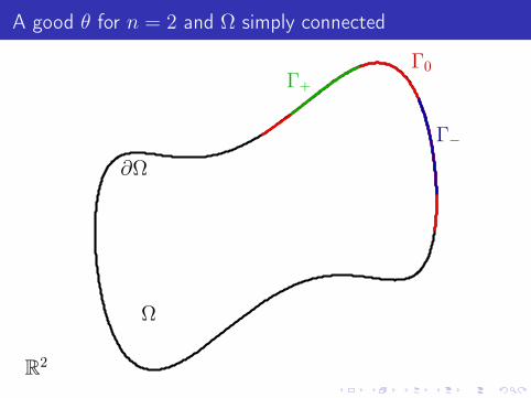
A good θ for n = 2 and Ω simply connected
Ω
∂Ω
R2
Γ0
A good θ for n = 2 and Ω simply connected
Ω
∂Ω
R2
Γ0
Γ−
Γ+

A good θ for n = 2 and Ω simply connected
Ω
∂Ω
R2
Γ0
Γ−
Γ+
g : ∂Ω → R∫
∂Ω gds = 0,
g > 0 = Γ+, g < 0 = Γ−

A good θ for n = 2 and Ω simply connected
Ω
∂Ω
R2
Γ0
Γ−
Γ+
g : ∂Ω → R∫
∂Ω gds = 0,
g > 0 = Γ+, g < 0 = Γ−
∆θ = 0,∂θ∂ν = g on ∂Ω

A good θ for n = 2 and Ω simply connected
Ω
∂Ω
R2
Γ0
Γ−
Γ+
g : ∂Ω → R∫
∂Ω gds = 0,
g > 0 = Γ+, g < 0 = Γ−
∆θ = 0,∂θ∂ν = g on ∂Ω
∇θ
From local controllability to global controllability
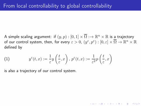
A simple scaling argument: if (y, p) : [0, 1] × Ω :→ Rn × R is a trajectory
of our control system, then, for every ε > 0, (yε, pε) : [0, ε] × Ω → Rn × R
defined by
yε(t, x) :=1
εy
(
t
ε, x
)
, pε(t, x) :=1
ε2p
(
t
ε, x
)
(1)
is also a trajectory of our control system.
Return method: references
Stabilization of driftless systems in finite dimension: JMC (1992).
Euler equations of incompressible fluids: JMC (1993,1996), O. Glass(1997,2000).
Control of driftless systems in finite dimension: E.D. Sontag (1995).
Navier-Stokes equations: JMC (1996), JMC and A. Fursikov (1996),A. Fursikov and O. Imanuvilov (1999), S. Guerrero, O. Imanuvilov andJ.-P. Puel (2006), JMC and S. Guerrero (2009), M. Chapouly (2009).
Burgers equation: Th. Horsin (1998), M. Chapouly (2006), O.Imanuvilov and J.-P. Puel (2009).
Saint-Venant equations: JMC (2002).
Vlasov Poisson: O. Glass (2003).

Return method: references (continued)
Isentropic Euler equations: O. Glass (2006).
Schrödinger equation: K. Beauchard (2005), K. Beauchard and JMC(2006).
Camassa-Holm equation: O. Glass (2008), V. Perrollaz (2010).
Korteweg de Vries equation: M. Chapouly (2008).
Hyperbolic equations: JMC, O. Glass and Z. Wang (2009).
Ensemble controllability of Bloch equations: K. Beauchard, JMC andP. Rouchon (2010).
Parabolic systems: JMC, S. Guerrero, L. Rosier (2010).
Uniform controllability of scalar conservation laws in the vanishingviscosity limit: M. Léautaud (2010).
The Navier-Stokes control system
The Navier-Stokes control system is deduced from the Euler equations byadding the linear term −∆y: the equation is now
yt −∆y + (y · ∇)y +∇p = 0, div y = 0.(1)
For the boundary condition, one requires now that
y = 0 on [0, T ]× (∂Ω \ Γ0).(2)
For the control, one can take, for example, y on [0, T ]× Γ0.
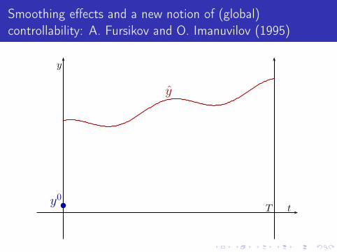
Smoothing effects and a new notion of (global)
controllability: A. Fursikov and O. Imanuvilov (1995)
T t
y
y
y0

Smoothing effects and a new notion of (global)
controllability: A. Fursikov and O. Imanuvilov (1995)
T t
y
y
y0

Smoothing effects and a new notion of local controllability
A. Fursikov and O. Imanuvilov (1995)
T t
y
y

Smoothing effects and a new notion of local controllability
A. Fursikov and O. Imanuvilov (1995)
T t
y
y

Smoothing effects and a new notion of local controllability
A. Fursikov and O. Imanuvilov (1995)
T t
y
y
y0

Smoothing effects and a new notion of local controllability
A. Fursikov and O. Imanuvilov (1995)
T t
y
y
y0

Local controllability
Theorem (A. Fursikov and O. Imanuvilov (1994), O. Imanuvilov(1998, 2001), E. Fernandez-Cara, S. Guerrero, O. Imanuvilov andJ.-P. Puel (2004))
The Navier-Stokes control system is locally controllable.
The proof relies on the controllability of the linearized control systemaround y (which is obtained by Carleman inequalities).
Global controllability
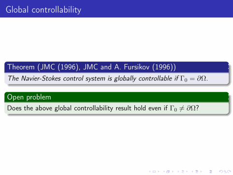
Theorem (JMC (1996), JMC and A. Fursikov (1996))
The Navier-Stokes control system is globally controllable if Γ0 = ∂Ω.
Open problem
Does the above global controllability result hold even if Γ0 6= ∂Ω?

Sketch of the proof of the global result
T
y
t

Sketch of the proof of the global result
T
y
t

Sketch of the proof of the global result
T
y
tB1 B2

Sketch of the proof of the global result
T
y
tB1 B2
y(t)

Sketch of the proof of the global result
T
y
tB1 B2
y(t)
B3 B4

The strategy explained on a finite dimensional case
We consider the following control system
y = F (y) +Bu(t),(1)
where the state is y ∈ Rn, the control is u ∈ R
m, B is a n×m matrix andF ∈ C1(Rn;Rn) is quadratic: F (λy) = λ2F (y), ∀λ ∈ [0,+∞), ∀y ∈ R
n.We assume that there exists a trajectory(y, u) ∈ C0([0, T0];R
n)× L∞((0, T0);Rm) of the control system (1) such
that the linearized control system around (y, u) is controllable and suchthat y(0) = y(T0) = 0.
Remark
One has F (0) = 0. Hence (0, 0) is an equilibrium of the control system(1). The linearized control system around this equilibrium is y = Bu, whichis not controllable if (and only if) B is not onto.

Let A be a n× n matrix and let us consider the following control system
y = Ay + F (y) +Bu(t),(1)
where the state is y ∈ Rn, the control is u ∈ R
m. For the application toincompressible fluids, (1) is the Euler control system and (1) is theNavier-Stokes control system.One has the following theorem.
Theorem
Under the above assumptions, the control system (1) is globallycontrollable in arbitrary time: For every T > 0, for every y0 ∈ R
n and forevery y1 ∈ R
n, there exists u ∈ L∞((0, T );Rm) such that
(
y = f(y, u(t)), y(0) = y0)
⇒(
y(T ) = y1)
.
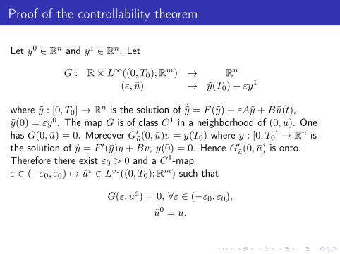
Proof of the controllability theorem
Let y0 ∈ Rn and y1 ∈ R
n. Let
G : R× L∞((0, T0);Rm) → R
n
(ε, u) 7→ y(T0)− εy1
where y : [0, T0] → Rn is the solution of ˙y = F (y) + εAy +Bu(t),
y(0) = εy0. The map G is of class C1 in a neighborhood of (0, u). Onehas G(0, u) = 0. Moreover G′
u(0, u)v = y(T0) where y : [0, T0] → Rn is
the solution of y = F ′(y)y +Bv, y(0) = 0. Hence G′u(0, u) is onto.
Therefore there exist ε0 > 0 and a C1-mapε ∈ (−ε0, ε0) 7→ uε ∈ L∞((0, T0);R
m) such that
G(ε, uε) = 0, ∀ε ∈ (−ε0, ε0),
u0 = u.

Let yε : [0, T0] → Rn be the solution of the Cauchy problem
˙yε = F (yε) + εAyε +Buε(t), yε(0) = εy0. Then yε(T0) = εy1. Lety : [0, εT0] → R
n and u : [0, εT0] → Rm be defined by
y(t) :=1
εyε
(
t
ε
)
, u(t) :=1
ε2uε
(
t
ε
)
.
Then y = F (y) +Ay +Bu, y(0) = y0 and y(εT0) = y1. This concludesthe proof of the controllability theorem if T is small enough. If T is notsmall, it suffices, with ε > 0 small enough, to go from y0 to 0 during theinterval of time [0, ε], stay at 0 during the interval of time [ε, T − ε] andfinally go from 0 to y1 during the interval of time [T − ε, T ].

Morality
The “morality” behind Theorem 4.4 is that the quadratic term F (y) winsagainst the linear term Ay. Note, however, that for Euler/Navier-Stokesequations the linear term µ∆y contains more derivatives than the quadraticterm (y · ∇)y. This creates many new difficulties and the proof requiresimportant modifications. In particular, one first gets a global approximatecontrollability result and then concludes with a local controllability result.Of course, as one can see by looking at the proof of the controllabilitytheorem, this method works only if we have a (good) convergence of thesolution of the Navier-Stokes equations to the solution of the Eulerequations when the viscosity tends to 0.

Let us recall that this is not known even in dimension n = 2 if there is nocontrol. More precisely, let us assume that Ω is of class C∞, that n = 2and that ϕ ∈ C∞
0 (Ω;R2) is such that div ϕ = 0. Let T > 0. Lety ∈ C∞([0, T ] × Ω;R2) and p ∈ C∞([0, T ]× Ω) be the solution to theEuler equations
(E)
yt + (y · ∇)y +∇p = 0, div y = 0, in (0, T ) × Ω,y · ν = 0 on [0, T ]× ∂Ω,
y(0, ·) = ϕ on Ω.
Let ε ∈ (0, 1]. Let yε ∈ C∞([0, T ] × Ω;R2) and pε ∈ C∞([0, T ] × Ω) bethe solution to the Navier-Stokes equations
(NS)
yεt − ε∆yε + (yε · ∇)yε +∇pε = 0, div yε = 0, in (0, T ) × Ω,yε = 0 on [0, T ]× ∂Ω,
y(0, ·) = ϕ on Ω.
One knows that there exists C > 0 such that |yε|C0([0,T ];L2(Ω;R2)) 6 C, forevery ε ∈ (0, 1].

One has the following challenging open problems.
Open problem (Convergence of Navier-Stokes to Euler)
(i) Does yε converge weakly to y in L2((0, T )× Ω;R2) as ε → 0+?
(ii) Let K be a compact subset of Ω and m be a positive integer. Doesyε|[0,T ]×K converge to y|[0,T ]×K in Cm([0, T ] ×K;R2) as ε → 0+?
(Of course, due to the difference of boundary conditions between theEuler equations and the Navier-Stokes equations, one does not have apositive answer to this last question if K = Ω.)

Main difficulty for the return method: Return to the initial
state
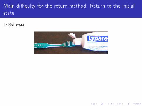
Main difficulty for the return method: Return to the initial
state
Initial state

Main difficulty for the return method: Return to the initial
state
Initial state
Intermediate state
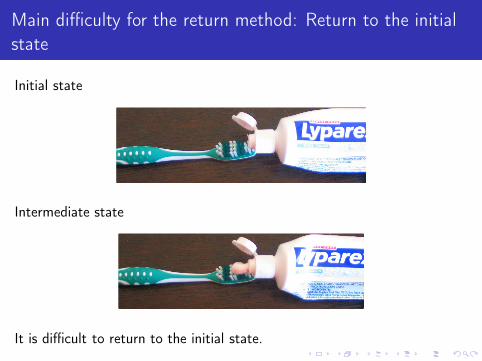
Main difficulty for the return method: Return to the initial
state
Initial state
Intermediate state
It is difficult to return to the initial state.

A water-tank control system

Saint-Venant equations: Notations
D
x
vH
The horizontal velocity v is taken with respect to the one of the tank.

The model: Saint-Venant equations
Ht + (Hv)x = 0, t ∈ [0, T ], x ∈ [0, L],(1)
vt +
(
gH +v2
2
)
x
= −u (t) , t ∈ [0, T ], x ∈ [0, L],(2)
v(t, 0) = v(t, L) = 0, t ∈ [0, T ],(3)
s(t) = u (t) , t ∈ [0, T ],(4)
D(t) = s (t) , t ∈ [0, T ].(5)
u (t) is the horizontal acceleration of the tank in the absolutereferential,
g is the gravity constant,
s is the horizontal velocity of the tank,
D is the horizontal displacement of the tank.

State space
d
dt
∫ L
0H (t, x) dx = 0,(1)
Hx(t, 0) = Hx(t, L) (= −u(t)/g).(2)
Definition (State space)
The state space (denoted Y) is the set of
Y = (H, v, s,D) ∈ C1([0, L]) × C1([0, L]) × R× R
satisfying
v(0) = v(L) = 0, Hx(0) = Hx(L),
∫ L
0H(x)dx = LHe.(3)

Main result
Theorem (JMC, (2002))
For T > 0 large enough the water-tank control system is locallycontrollable in time T around (Ye, ue) := ((He, 0, 0, 0), 0).
Prior work: F. Dubois, N. Petit and P. Rouchon (1999):
1 The linearized control system around (Ye, ue) is not controllable,
2 Steady state controllability of the linearized control system around(Ye, ue).

Corollary 1: Destroy waves
u

Corollary 2: Steady-state controllability
D1
u
The linearized control system
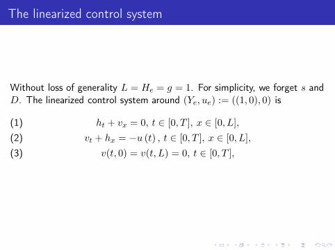
Without loss of generality L = He = g = 1. For simplicity, we forget s andD. The linearized control system around (Ye, ue) := ((1, 0), 0) is
ht + vx = 0, t ∈ [0, T ], x ∈ [0, L],(1)
vt + hx = −u (t) , t ∈ [0, T ], x ∈ [0, L],(2)
v(t, 0) = v(t, L) = 0, t ∈ [0, T ],(3)

The linearized control system is not controllable
For a function w : [0, 1] → R, we denote by wev “the even part”of w and bywod the odd part of w:
wev(x) :=1
2(w(x) + w(1 − x)), wod(x) :=
1
2(w(x) − w(1− x)).
Σ1
hodt + vev
x = 0,
vevt + hod
x = −u (t) ,vev(t, 0) = vev(t, 1) = 0,
Σ2
hevt + vod
x = 0,
vodt + hev
x = 0,
vod(t, 0) = vod(t, 1) = 0,
The Σ2 part is clearly not controllable.
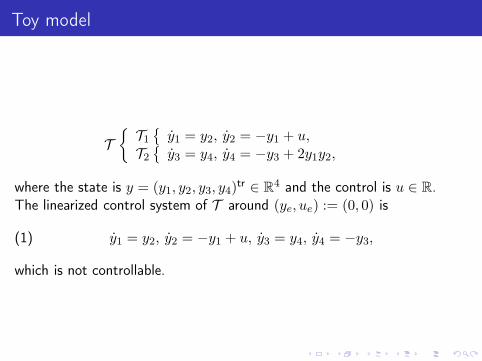
Toy model
T
T1
y1 = y2, y2 = −y1 + u,T2
y3 = y4, y4 = −y3 + 2y1y2,
where the state is y = (y1, y2, y3, y4)tr ∈ R
4 and the control is u ∈ R.The linearized control system of T around (ye, ue) := (0, 0) is
y1 = y2, y2 = −y1 + u, y3 = y4, y4 = −y3,(1)
which is not controllable.

Controllability of the toy model
If y(0) = 0,
y3(T ) =
∫ T
0y21(t) cos(T − t)dt,(1)
y4(T ) = y21(T )−
∫ T
0y21(t) sin(T − t)dt.(2)
Hence T is not controllable in time T 6 π. Using explicit computationsone can show that T is (locally) controllable in time T > π.
Remark
For linear systems in finite dimension, the controllability in large timeimplies the controllability in small time. This is no longer for linear PDE.This is also no longer true for nonlinear systems in finite dimension.

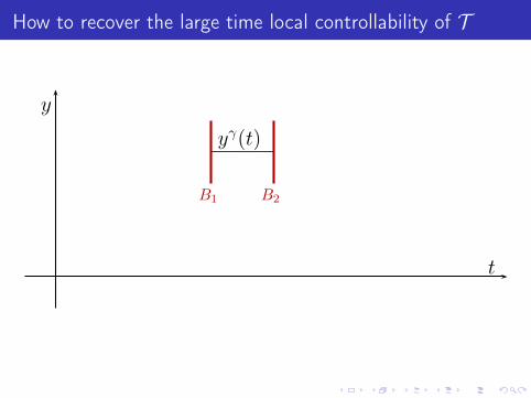
How to recover the large time local controllability of T
The first point is at least to find a trajectory such that the linearizedcontrol system around it is controllable. We try the simplest possibletrajectories, namely equilibrium points. Let γ ∈ R and define
((yγ1 , yγ2 , y
γ3 , y
γ4 )
tr, uγ) := ((γ, 0, 0, 0)tr , γ).(1)
Then ((yγ1 , yγ2 , y
γ3 , y
γ4 )
tr, uγ) is an equilibrium of T . The linearized controlsystem of T at this equilibrium is
y1 = y2, y2 = −y1 + u, y3 = y4, y4 = −y3 + 2γy2,(2)
which is controllable if (and only if) γ 6= 0.

How to recover the large time local controllability of T
y
t

How to recover the large time local controllability of T
y
t
yγ(t)
How to recover the large time local controllability of T
y
t
yγ(t)
B1 B2

How to recover the large time local controllability of T
y
t
yγ(t)
B1 B2

How to recover the large time local controllability of T
y
t
yγ(t)
B1 B2

How to recover the large time local controllability of T
y
t
yγ(t)
B1 B2
B0 a

How to recover the large time local controllability of T
y
t
yγ(t)
B1 B2
B0 a

How to recover the large time local controllability of T
y
t
yγ(t)
B1 B2
B0 a B3
T
b

Construction of the blue trajectory
One uses quasi-static deformations. Let g ∈ C2([0, 1];R) be such that
g(0) = 0, g(1) = 1.
Let u : [0, 1/ε] → R be defined by
u(t) := γg(εt), t ∈ [0, 1/ε].
Let y := (y1, y2, y3, y4)tr : [0, 1/ε] → R
4 be defined by requiring
˙y1 = y2, ˙y2 = −y1 + u, ˙y3 = y4, ˙y4 = −y3 + 2y1y2,(1)
y(0) = 0.(2)
One easily checks that
y(1/ε) → (γ, 0, 0, 0)tr as ε → 0.

(yγ, uγ) for the water-tank
u(t) = γ, h = γ
(
1
2− y
)
, v = 0.

Difficulties
Loss of derivatives. Solution: one uses the iterative scheme inspired bythe usual one to prove the existence to yt +A(y)yx = 0, y(0, x) = ϕ(x),namely
Σnlinear : yn+1t +A(yn)yn+1
x = 0, yn+1(0, x) = ϕ(x).
However, I have only been able to prove that the control systemcorresponding to Σnlinear is controllable for (hn, vn) satisfying someresonance conditions. Hence one has also to insure that (hn+1, vn+1)satisfies these resonance conditions. This turns out to be possible. (Forcontrol system, resonance is good: when there is a resonance, with a smallaction we get a strong effect).
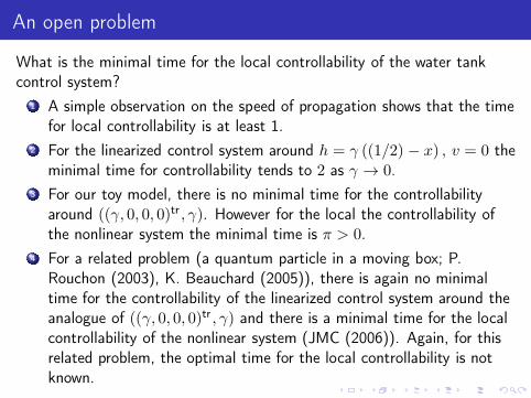
An open problem
What is the minimal time for the local controllability of the water tankcontrol system?
1 A simple observation on the speed of propagation shows that the timefor local controllability is at least 1.
2 For the linearized control system around h = γ ((1/2) − x) , v = 0 theminimal time for controllability tends to 2 as γ → 0.
3 For our toy model, there is no minimal time for the controllabilityaround ((γ, 0, 0, 0)tr , γ). However for the local the controllability ofthe nonlinear system the minimal time is π > 0.
4 For a related problem (a quantum particle in a moving box; P.Rouchon (2003), K. Beauchard (2005)), there is again no minimaltime for the controllability of the linearized control system around theanalogue of ((γ, 0, 0, 0)tr , γ) and there is a minimal time for the localcontrollability of the nonlinear system (JMC (2006)). Again, for thisrelated problem, the optimal time for the local controllability is notknown.
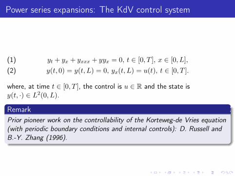
Power series expansions: The KdV control system
yt + yx + yxxx + yyx = 0, t ∈ [0, T ], x ∈ [0, L],(1)
y(t, 0) = y(t, L) = 0, yx(t, L) = u(t), t ∈ [0, T ].(2)
where, at time t ∈ [0, T ], the control is u ∈ R and the state isy(t, ·) ∈ L2(0, L).
Remark
Prior pioneer work on the controllability of the Korteweg-de Vries equation(with periodic boundary conditions and internal controls): D. Russell andB.-Y. Zhang (1996).
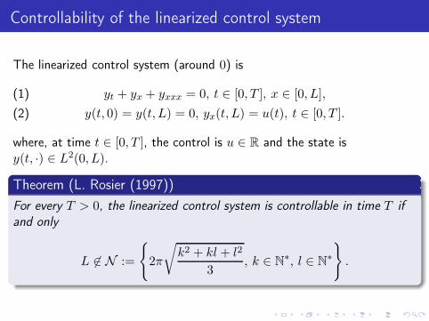
Controllability of the linearized control system
The linearized control system (around 0) is
yt + yx + yxxx = 0, t ∈ [0, T ], x ∈ [0, L],(1)
y(t, 0) = y(t, L) = 0, yx(t, L) = u(t), t ∈ [0, T ].(2)
where, at time t ∈ [0, T ], the control is u ∈ R and the state isy(t, ·) ∈ L2(0, L).
Theorem (L. Rosier (1997))
For every T > 0, the linearized control system is controllable in time T ifand only
L 6∈ N :=
2π
√
k2 + kl + l2
3, k ∈ N
∗, l ∈ N∗
.
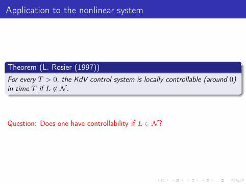
Application to the nonlinear system
Theorem (L. Rosier (1997))
For every T > 0, the KdV control system is locally controllable (around 0)in time T if L 6∈ N .
Question: Does one have controllability if L ∈ N ?

Controllability when L ∈ N
Theorem (JMC and E. Crépeau (2004))
If L = 2π (which is in N : take k = l = 1), for every T > 0 the KdVcontrol system is locally controllable (around 0) in time T .
Theorem (E. Cerpa (2007), E. Cerpa and E. Crépeau (2008))
For every L ∈ N , there exists T > 0 such that the KdV control system islocally controllable (around 0) in time T .

Strategy of the proof: power series expansion.
Example with L = 2π. For every trajectory (y, u) of the linearized controlsystem around 0
d
dt
∫ 2π
0(1− cos(x))y(t, x)dx = 0.
This is is the only “obstacle” to the controllability of the linearized controlsystem:
Proposition (L. Rosier (1997))
Let H := y ∈ L2(0, L);∫ L0 (1− cos(x))y(x)dx = 0. For every
(y0, y1) ∈ H ×H, there exists u ∈ L2(0, T ) such that the solution to theCauchy problem
yt + yx + yxxx = 0, y(t, 0) = y(t, L) = 0, yx(t, L) = u(t), t ∈ [0, T ],
y(0, x) = y0(x), x ∈ [0, L],
satisfies y(T, x) = y1(x), x ∈ [0, L].

We explain the method on the control system of finite dimension
y = f(y, u),
where the state is y ∈ Rn and the control is u ∈ R
m. We assume that(0, 0) ∈ R
n × Rm is an equilibrium of the control system y = f(y, u), i.e.
that f(0, 0) = 0. Let
H := Span AiBu; u ∈ Rm, i ∈ 0, . . . , n − 1
with
A :=∂f
∂y(0, 0), B :=
∂f
∂u(0, 0).
If H = Rn, the linearized control system around (0, 0) is controllable and
therefore the nonlinear control system y = f(y, u) is small-time locallycontrollable at (0, 0) ∈ R
n × Rm.
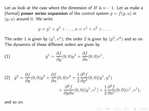
Let us look at the case where the dimension of H is n− 1. Let us make a(formal) power series expansion of the control system y = f(y, u) in(y, u) around 0. We write
y = y1 + y2 + . . . , u = v1 + v2 + . . . .
The order 1 is given by (y1, v1); the order 2 is given by (y2, v2) and so on.The dynamics of these different orders are given by
y1 =∂f
∂y(0, 0)y1 +
∂f
∂u(0, 0)v1,(1)
(2) y2 =∂f
∂y(0, 0)y2 +
∂f
∂u(0, 0)v2 +
1
2
∂2f
∂y2(0, 0)(y1, y1)
+∂2f
∂y∂u(0, 0)(y1, v1) +
1
2
∂2f
∂u2(0, 0)(v1, v1),
and so on.

Let e1 ∈ H⊥. Let T > 0. Let us assume that there are controls v1± andv2±, both in L∞((0, T );Rm), such that, if y1± and y2± are solutions of
y1± =∂f
∂y(0, 0)y1± +
∂f
∂u(0, 0)v1±,(1)
y1±(0) = 0,(2)
(3) y2± =∂f
∂y(0, 0)y2± +
∂f
∂u(0, 0)v2± +
1
2
∂2f
∂y2(0, 0)(y1±, y
1±)
+∂2f
∂y∂u(0, 0)(y1±, u
1±) +
1
2
∂2f
∂u2(0, 0)(u1±, u
1±),
y2±(0) = 0,(4)
then
y1±(T ) = 0,(5)
y2±(T ) = ±e1.(6)

Let (ei)i∈2,...n be a basis of H. By the definition of H, there are(ui)i=2,...,n, all in L∞(0, T )m, such that, if (yi)i=2,...,n are the solutions of
yi =∂f
∂y(0, 0)yi +
∂f
∂u(0, 0)ui,(1)
yi(0) = 0,(2)
then, for every i ∈ 2, . . . , n,
yi(T ) = ei.(3)
Now let
b =n∑
i=1
biei(4)
be a point in Rn. Let v1 and v2, both in L∞((0, T );Rm), be defined by
the following
If b1 > 0, then v1 := v1+ and v2 := v2+,(5)
If b1 < 0, then v1 := v1− and v2 := v2−.(6)

Let u : (0, T ) → Rm be defined by
u(t) := |b1|1/2v1(t) + |b1|v
2(t) +
n∑
i=2
biui(t).(1)
Let y : [0, T ] → Rn be the solution of
y = f(y, u(t)), y(0) = 0.(2)
Then one has, as b → 0,
y(T ) = b+ o(b).(3)
Hence, using the Brouwer fixed-point theorem and standard estimates onordinary differential equations, one gets the local controllability ofy = f(y, u) (around (0, 0) ∈ R
n × Rm) in time T , that is, for every ε > 0,
there exists η > 0 such that, for every (a, b) ∈ Rn × R
n with |a| < η and|b| < η, there exists a trajectory (y, u) : [0, T ] → R
n × Rm of the control
system y = f(y, u) such that
y(0) = a, y(T ) = b,(4)
|u(t)| 6 ε, t ∈ (0, T ).(5)
Bad and good news for L = 2π
• Bad news: The order 2 is not sufficient. One needs to go to the order3
• Good news: the fact that the order is odd allows to get the localcontrollability in arbitrary small time. The reason: If one can move inthe direction ξ ∈ H⊥ one can move in the direction −ξ. Hence itsuffices to argue by contradiction (assume that it is impossible toenter in H⊥ in small time etc.)

Open problems
1 Is there a minimal time for local controllability for some values of L?
2 Do we have global controllability? This is open even with threeboundary controls:
yt + yx + yxxx + yyx = 0,(1)
y(t, 0) = u1(t), y(t, L) = u2(t), yx(t, L) = u3(t).(2)
Note that one has global controllability for
yt + yx + yxxx + yyx = u4(t),(3)
y(t, 0) = u1(t), y(t, L) = u2(t), yx(t, L) = u3(t).(4)
(M. Chapouly (2009)). The proof uses the return method as for theNavier-Stokes control system.