control strategies and parameter compensation for permanent
TRANSCRIPT
Control Strategies and ParameterCompensation for Permanent Magnet
Synchronous Motor Drives
Ramin Monajemy
Dissertation Submitted to the Faculty of the Virginia Polytechnic Institute andState University in Partial Fulfillment of the Requirements for the degree of
Doctor of PhilosophyIn
Electrical Engineering
Krishnan Ramu, ChairmanHugh VanLandinghamWilliam T. BaumannCharles E. NunnallyLance A. Matheson
October 12, 2000Blacksburg, Virginia
Key Words: Motor Drives, Permanent Magnet Synchronous Motor, ControlStrategies, Operational Boundary, Power Losses
Copyright 2000, Ramin Monajemy

Control Strategies and Parameter Compensation forPermanent Magnet Synchronous Motor Drives
Ramin Monajemy
(Abstract)
Variable speed motor drives are being rapidly deployed for a vast range of applications in order
to increase efficiency and to allow for a higher level of control over the system. One of the
important areas within the field of variable speed motor drives is the system’s operational
boundary. Presently, the operational boundaries of variable speed motor drives are set based on
the operational boundaries of single speed motors, i.e. by limiting current and power to rated
values. This results in under-utilization of the system, and places the motor at risk of excessive
power losses. The constant power loss (CPL) concept is introduced in this dissertation as the
correct basis for setting and analyzing the operational boundary of variable speed motor drives.
The control and dynamics of the permanent magnet synchronous motor (PMSM) drive operating
with CPL are proposed and analyzed. An innovative implementation scheme of the proposed
method is developed. It is shown that application of the CPL control system to existing systems
results in faster dynamics and higher utilization of the system. The performance of a motor drive
with different control strategies is analyzed and compared based on the CPL concept. Such
knowledge allows for choosing the control strategy that optimizes a motor drive for a particular
application. Derivations for maximum speed, maximum current requirements, maximum torque
and other performance indices, are presented based on the CPL concept. High performance
drives require linearity in torque control for the full range of operating speed. An analysis of
concurrent flux weakening and linear torque control for PMSM is presented, and implementation
strategies are developed for this purpose. Implementation strategies that compensate for the
variation of machine parameters are also introduced. A new normalization technique is
introduced that significantly simplifies the analysis and simulation of a PMSM drive's
performance. The concepts presented in this dissertation can be applied to all other types of
machines used in high performance applications. Experimental work in support of the key
claims of this dissertation is provided.

iii
Dedication
I dedicate this dissertation to my father, mother and sister who believed in me all through these
years, and provided outstanding moral support.

iv
Acknowledgements
I would like to thank my advisor, Professor Krishnan Ramu, for providing guidance and sharing
his vision and experiences throughout the development of this dissertation. Many thanks also
goes to my committee members, Professor VanLandingham, Professor Baumann, Professor
Nunnally and Professor Matheson, for monitoring this effort and for providing their valuable
opinions.
I would like to thank the members of the MCSRG group for the many discussions that we had
and for sharing their opinion on different subjects. I would like to acknowledge and thank
former Ph.D. student, Dr. Nishith Tripathi, for assisting me in preparing and training the neural
networks that are used in this dissertation.
v
Table of Contents
List of Figures x
Symbols and Abbreviations xiii
1 Introduction 1
1.1 Foreword 1
1.2 Areas of Interest and Research Outline 2
1.3 Drawbacks of Existing Control Techniques 4
1.3.1 Under-utilization in the Lower than Base Speed Range 4
1.3.2 Excessive Power Losses in the Flux Weakening Range 5
1.3.3 Torque Non-linearity Caused by Ignoring Core Losses 5
1.3.4 Torque Non-linearity Caused by Improper Implementation 5
1.3.5 Confusion in the Definition of Base Speed 6
1.4 Advantages of the Techniques Presented in this dissertation 6
1.5 Potential Impact on the Research Community and Industry 7
1.6 Dissertation Structure 7
1.7 Summary of Contributions and List of Co-authored Papers 8
1.8 Assumptions 9
1.9 Conclusions 10
2 State of the Art 11
2.1 Introduction 11
2.2 The Electric Motor: A Historical Perspective 11
2.3 Trends Forcing the Transition to Variable Speed Drives 15
2.4 Why Concentrate this Study on PMSM? 17
2.5 Literature Review 17
2.5.1 Power Losses and Efficiency 18
2.5.2 Operational Boundaries of Motor Drives 19
2.5.3 Control Strategies for Operation Below Base Speed 19
2.5.4 Control Strategies for Operation Above Base Speed 21

vi
2.5.5 Parameter Sensitivity and Parameter Insensitive Control Strategies 22
2.6 Conclusions 23
3 Control and Dynamics of Constant Power Loss Based Operation of PMSM 24
3.1 Introduction 24
3.2 PMSM Model with Losses 26
3.2.1 Electrical Equations of PMSM Including Core Losses 27
3.2.2 Total Power Loss Equation for PMSM 28
3.3 Constant Power Loss Control Scheme and Comparison 28
3.3.1 The Lower than Base Speed Operating Range 31
3.3.2 The Flux Weakening Operating Range 31
3.4 Secondary Issues of the CPL Controller 32
3.4.1 Higher Current Requirement at Lower than Base Speed 32
3.4.2 Parameter Dependency 32
3.5 Implementation Scheme for the CPL Controller 33
3.6 Experimental Correlation 34
3.7 The Drive Control with Power Loss Command 35
3.7.1 Cycling the Drive 35
3.7.2 Commanding Short Term Maximum Torque 36
3.8 Conclusions 38
4 The CPL Controller for Applications with Cyclic Loads 39
4.1 Introduction 39
4.2 The Power Loss Command in Different Application Categories 40
4.2.1 Derivation of a Practical Power Loss Estimator 40
4.2.2 Power Loss Command and Maximum Torque in
Different Application Categories 41
4.3 Comparison of Maximum Torque in Different Load Categories 51
4.3.1 Load Categories A to D 51
4.3.2 Load Category E 53
4.4 Conclusions 53

vii
5 Performance Evaluation and Comparison of Control Strategies 55
5.1 Introduction 55
5.2 Performance Criteria 57
5.3 Control Strategies: Lower than Base Speed Operating Range 59
5.3.1 Maximum Efficiency Control Strategy 61
5.3.2 Zero D-Axis Current Control Strategy 62
5.3.3 Maximum Torque per Unit Current Control Strategy 63
5.3.4 Unity Power Factor Control Strategy 63
5.3.5 Constant Mutual Flux Linkages Control Strategy 64
5.4 Control Strategies: Higher than Based Speed Operating Range 65
5.4.1 Constant Back EMF Control Strategy 66
5.4.2 Six Step Voltage Control Strategy 69
5.5 Comparison of Control Strategies Based on the CPL Concept 74
5.5.1 Lower than Base Speed Operating Range 74
5.5.2 Higher than Base Speed Operating Range 80
5.6 Performance Comparison inside the Operational Envelope 84
5.6.1 Current vs. Torque 85
5.6.2 Air Gap Flux Linkages vs. Torque 85
5.6.3 Power Factor vs. Torque 85
5.6.4 D-Axis Current vs. Torque 87
5.6.5 Torque Range 87
5.7 Direct Steady State Evaluation in SSV Mode 87
5.8 Simulation and Experimental Verification 91
5.9 Conclusions 93
6 Analysis and Implementation of Concurrent Mutual Flux Weakening and Torque
Control for PMSM 95
6.1 Introduction 95
6.2 Mutual Flux Linkages Weakening Strategy and Control 96
6.2.1 The Mutual Flux Linkages Weakening Strategy 96
6.2.2 Mutual Flux Linkages and Torque Control 96

viii
6.3 Maximum Torque for a Given Mutual Flux Linkages 97
6.4 Controller Block Diagram 98
6.5 Implementation Strategies 100
6.5.1 Lookup Table Approach 100
6.5.2 Two-Dimensional Polynomials Approach 103
6.6 Comparison of the Two Approaches 105
6.7 Conclusions 106
7 Concurrent Mutual Flux Weakening and Torque Control in the Presence of Parameter
Variations 107
7.1 Introduction 107
7.2 The Variation of Parameters in PMSM 108
7.3 The Impact of Parameter Variations 109
7.4 Parameter Compensation Scheme 111
7.4.1 Lookup Table Approach 112
7.4.2 Artificial Neural Network Approach 113
7.5 Comparison of the Two Approaches 114
7.6 Dynamic Simulation 115
7.7 Estimation of Machine Parameters 117
7.8 Conclusions 118
8 Applications of a New Normalization Technique 119
8.1 Introduction 119
8.2 The New Normalization Technique 120
8.3 Comparison to other Normalization Techniques 122
8.4 Derivation of Maximum Torque vs. Speed Envelopes 123
8.4.1 The Maximum Efficiency Control Strategy 123
8.4.2 The Maximum Torque per Unit Current Control Strategy 125
8.4.3 The Zero D-Axis Current Control Strategy 125
8.4.4 The Unity Power Factor Control Strategy 126
8.4.5 The Constant Mutual Flux Linkages Control Strategy 126
ix
8.4.6 The Constant Back EMF Control Strategy 127
8.5 Derivation of Maximum Current Requirement with CPL 128
8.6 Maximum Possible Torque as a Function of Flux Linkages 129
8.7 Generalized Performance Characteristics 131
8.8 Conclusions 135
9 Conclusions and Recommendations for Future Work 136
9.1 Conclusions 136
9.2 Recommendations for Future Work 138
Appendix I Prototype PMSM Drive 139
Appendix II Measurement of PMSM Parameters 140
References 143
Vita 150
x
List of Figures
Figure 3.1. q and d axis steady-state model in rotor reference frame includingstator and core loss resistances. 27
Figure 3.2. Normalized maximum torque, power loss, air gap power, voltageand phase current vs. speed for the CPLC (solid lines) and for thescheme with current and power limited to rated values(dashed lines). 30
Figure 3.3. Implementation scheme for the constant power loss controller. 33
Figure 3.4. Current, torque, estimated torque, total power loss, copper andcore losses along the CPLC boundary with power loss referenceof 30 W. 36
Figure 3.5. Dynamic response of the system for a step torque command of1.5 N.m. 37
Figure 3.6. Simulated speed, mω (RPM), and phase current command,*aI (A), in response to 1.5 N.m. step torque command. 37
Figure 4.1. Normalized torque, eT , and speed, rω , profiles for continuous
operation. 42
Figure 4.2. Normalized torque and speed profiles for on-off operation withsmall transition times. 44
Figure 4.3. Normalized torque and speed profiles for speed reversal application. 46
Figure 4.4. Normalized torque and speed profiles for operation between rmω± . 47
Figure 4.5. Normalized torque and speed profiles for operation with significanttransition times. 49
Figure 4.6. Maximum torque vs. maximum power loss for load categories A, B, C and D forduty cycles equal to 1, 0.75, 0.5, 0.33. 52
Figure 5.1. Normalized motor variables in steady state for a six step voltage inputvs. rotor angle in electrical degrees at 1635 RPM and dc bus voltageof 65 Volts and voltage phasor angle of 116 degrees. 73
xi
Figure 5.2. Maximum torque, current, power and net loss vs. speed at ratedpower loss for lower than base speed control strategies, and
1.1Em = p.u. for the flux weakening range. 76
Figure 5.3. Torque per current, back emf, power factor and net loss vs. speedat rated power loss for lower than base speed control strategies,and 1.1Em = p.u. for the flux weakening region. 77
Figure 5.4. Maximum torque, peak current, net power loss, torque ripple asa percentage of average torque, and peak to peak torque ripplefor SSV (solid lines) and CBE (dashed lines, mE =0.8 p.u.)control strategies. 82
Figure 5.5. Current, air gap flux linkages, power factor and d-axis currentvs. torque for different control strategies. ( 85.2L/L dq = ) 86
Figure 5.6. Estimated (dashed lines) and measured (solid lines) maximumtorque vs. speed trajectory for the SSV and CBE controlstrategies with maximum power loss of 30 W and .V65Vdc = 92
Figure 5.7. Measured phase voltage and current for the SSV control strategyat 1635 RPM, 116=α degrees and =dcV 65 V. 92
Figure 5.8. Simulated phase voltage and current for the SSV control strategyat 1635 RPM, 116=α degrees and =dcV 65 V. 93
Figure 6.1. Maximum permissible torque command as a function of mutualflux linkages command. 98
Figure 6.2. Controller block diagram for the flux weakening range. 99
Figure 6.3. Controller block diagram for the lower than base speed operatingrange. 99
Figure 6.4. *qni as a function of normalized mutual flux linkages and torque
commands. 102
Figure 6.5. *dni as a function of normalized mutual flux linkages and torque
commands. 102
Figure 6.6. Normalized speed, torque, mutual flux linkages, and phasevoltage for a ± 3 p.u. step speed command. 104

xii
Figure 6.7. Commanded and achieved mutual flux linkages vs. commandedtorque for the polynomial implementation approach. 105
Figure 7.1. The mutual flux linkages and torque control system. 109
Figure 7.2. Normalized torque error when p.u.8.0af =λ 111
Figure 7.3. Mutual flux linkages error when p.u.8.0af =λ 111
Figure 7.4. The mutual flux linkages and torque control with compensationfor a varying parameter. 112
Figure 7.5. The ANN based offset generator structure. 114
Figure 7.6. Commanded and actual values for speed, torque, mutual fluxlinkages, q and d-axis currents and phase voltage for a ± 3 p.u. speedcommand in the presence of 20 percent reduction in rotor flux linkages. 116
Figure 7.7. Commanded and actual values for mutual flux linkages and torque for a± 3 p.u. speed command in the presence of a 20 percentreduction in q-axis inductance. 117
Figure 8.1. Generalized application characteristics for PMSM with 3,2,1=ρ for the 132maximum torque per unit current control strategy.
Figure 8.2. Generalized application characteristics for PMSM with 3,2,1=ρ for the 134zero d-axis current control strategy.

* Any of the variables shown here can be used with a subscript n to denote normalization.
Symbols and Abbreviations
α angle of stator voltage phasor with respect to rotor's d-axisd duty cycleE back emf
mE maximum desired back emf
Er
back emf phasorη efficiency
I torque generating portion of stator current magnitude (steady state)
Ir
current phasor
bI base value for current
cI core loss portion of stator current magnitude (steady state)
dq I,I q and d axis torque generating currents, respectively (steady state)
dcqc I,I q and d axis core loss currents, respectively (steady state)
dmqm I,I maximum q and d axis currents, respectively
dsqs I,I q and d axis stator currents, respectively (steady state)
sI stator current magnitude (steady state)
smI maximum stator current magnitude
srI rated current
ai phase a current*ai phase a current command
c,b,ai phase a, b, c currents
dsqs i,i q and d axis stator currents, respectively
*ds
*qs i,i q and d axis stator current commands, respectively
*ds
*qs i,i nominal q and d axis stator current commands, respectively
dq i,i q and d axis torque generating currents, respectively
si stator current magnitude*d
*q i,i ∆∆ q and d axis current command offsets, respectively
tK motor torque constant
dq L,L q and d-axis inductances, respectively
bL base value for inductance

xiv
mλ mutual (or air gap) flux linkages
bλ base value for flux linkages*mλ mutual (or air gap) flux linkages command
afλ rotor flux linkages
afeλ rotor flux linkages estimation
afλ nominal value of rotor flux linkages
mλ∆ mutual flux linkages error
rω electrical speed*rω commanded speed
rrω rated speed
bω base value for speed
mω measured speed
rmω maximum speed
lmP maximum permissible power loss
ldlq P,P q and d axis power losses, respectively
lcP total core losses*lP power loss command
lP power losses
lP average power losses
lfP filtered power losses estimation
aP air gap power
rP rated power
bP base value for power
P number of poles
lrP total copper and core losses at rated speed and torque
sR , cR stator and core loss resistors, respectively
ρ ratio of q and d axis inductances (saliency ratio)T cycle period
offT off time (in one period)
onT on time (in one period)
1pT∆ rise time
2pT∆ fall time
mT∆ time during which constant torque is applied
zT∆ time during which no torque is applied
eT air gap torque
xv
*eT commanded torque*eT
~commanded torque after being limited
ebT base value for torque
emT maximum air gap torque
epT peak air gap torque
limT torque limit
eT∆ torque error
mθ measured rotor position
rθ rotor electrical position
bV base value for voltage
dcV dc bus voltage
mV fundamental component of stator voltage magnitude
dsqs V,V q and d axis stator voltages, respectively (steady state)
sV stator voltage magnitude (steady state)
smV maximum stator voltage magnitude
av phase a voltage
dsqs v,v q and d axis stator voltages, respectively
lW energy losses in one period
BDCM brushless dc motorCBE constant back emf (control strategy)CMFL constant mutual flux linkages (control strategy)CPL constant power lossCPLC constant power loss controllerDAC digital to analog converterMTPC maximum torque per unit current (control strategy)PI proportional integrator (controller)PMSM permanent magnet synchronous motorpf power factorSSV six-step voltage (control strategy)UPF unity power factor (control strategy)ZDAC zero d-axis current (control strategy)

1
CHAPTER 1
Introduction
1.1 FOREWORD
For the better part of the 20th century most motion control systems were designed to operate at
a fixed speed. Many existing systems still operate based on a speed determined by the frequency
of the power grid. However, the most efficient operating speed for many applications, such as
fans, blowers and centrifugal pumps, is different from that enforced by the grid frequency. Also,
many high performance applications, such as robots, machine tools and the hybrid vehicle,
require variable speed operation to begin with. As a result, a major transition from single speed
systems to variable speed systems is in progress. The transition from single speed drives to
variable speed drives has been in effect since the 1970s when movements towards conservation
of energy and protection of the environment were initiated. About seventy percent of all
electrical energy is converted into mechanical energy by motors in the industrialized world. This
may be the most important factor behind today’s high demand for more efficient motion control
systems. A large body of research is available on variable speed drives due to the significant
industrial and commercial interest in such systems. However, some areas of importance merit
further investigation. One such area is the operational boundary of motor drives. The
operational boundaries of variable speed motor drives are being incorrectly set based on the
operational boundaries of single speed motor drives, i.e. by limiting current and power to rated
values. The operational boundary of any motor drive must be set based on the maximum
possible power loss vs. speed profile for the given motor. Also, all control strategies for a
machine must be analyzed and compared based on such an operational boundary.
The areas of interest in this dissertation are discussed in section 1.2. The drawbacks of existing
control techniques for high performance control of PMSM are discussed in section 1.3. The
advantages of the techniques developed in this dissertation are discussed in section 1.4. The
potential impact of this research effort on the research community and on the industry is

Chapter 1 Introduction 2
discussed in section 1.5. The structure of this dissertation is presented in section 1.6. The
summary of key contributions of this dissertation are given in section 1.7. The assumptions are
discussed in section 1.8. The conclusions are summarized in section 1.9.
1.2 AREAS OF INTEREST AND RESEARCH OUTLINE
The emphasis of this dissertation is on high performance control strategies for variable speed
motor drives. High performance control strategies are capable of providing accurate control over
torque or speed to within a small percentage error. A high performance control strategy can also
optimize one or more performance indices such as torque, efficiency and power factor. The
following areas are of particular interest within the scope of high performance motor drives:
• Operational boundary of motor drives
• Implementation strategies that automatically limit the operational boundary for the full range
of operational speed based on a desired power loss profile
• Performance of different torque control strategies based on operation under constant power
loss
• Implementation strategies for concurrent flux weakening and torque control
• Parameter insensitive control strategies for concurrent flux weakening and torque control
• Innovative normalization techniques that simplify the analysis and simulation of motor drive
performance
The operational boundary of a machine is generally defined by the rated current and power of
the machine. This operational boundary is only valid at rated speed. However, the same
operational boundary has been wrongly carried over to variable speed motor drives. The true
operational boundary of a machine depends on the maximum permissible power loss profile for
the machine. Copper and core losses are the most fundamental sources of power losses in a
machine. Core losses are more significant than copper losses at higher speeds. A
comprehensive study of the operational boundaries of motor drives is performed in this
dissertation. Both copper and core losses are taken into account. The constant power loss (CPL)
concept is introduced here as a basis for defining the operational boundary of a motor drive. The
control and dynamics of the permanent magnet synchronous motor (PMSM) drive operating
Chapter 1 Introduction 3
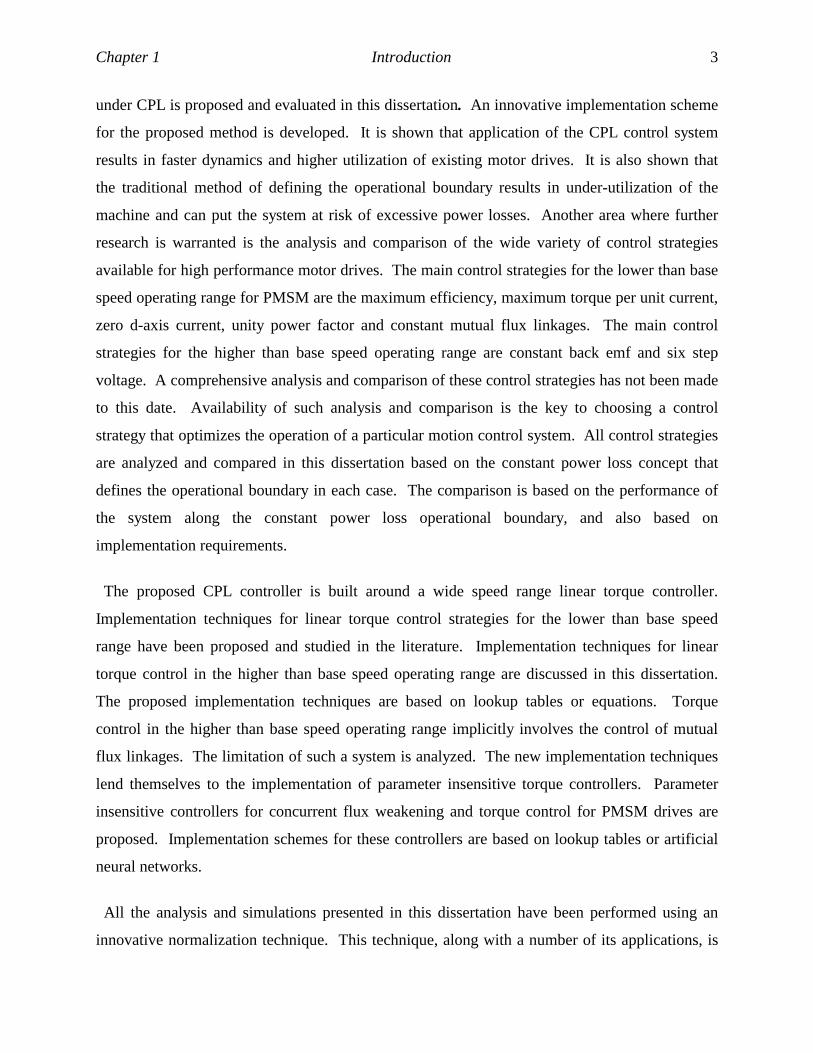
under CPL is proposed and evaluated in this dissertation. An innovative implementation scheme
for the proposed method is developed. It is shown that application of the CPL control system
results in faster dynamics and higher utilization of existing motor drives. It is also shown that
the traditional method of defining the operational boundary results in under-utilization of the
machine and can put the system at risk of excessive power losses. Another area where further
research is warranted is the analysis and comparison of the wide variety of control strategies
available for high performance motor drives. The main control strategies for the lower than base
speed operating range for PMSM are the maximum efficiency, maximum torque per unit current,
zero d-axis current, unity power factor and constant mutual flux linkages. The main control
strategies for the higher than base speed operating range are constant back emf and six step
voltage. A comprehensive analysis and comparison of these control strategies has not been made
to this date. Availability of such analysis and comparison is the key to choosing a control
strategy that optimizes the operation of a particular motion control system. All control strategies
are analyzed and compared in this dissertation based on the constant power loss concept that
defines the operational boundary in each case. The comparison is based on the performance of
the system along the constant power loss operational boundary, and also based on
implementation requirements.
The proposed CPL controller is built around a wide speed range linear torque controller.
Implementation techniques for linear torque control strategies for the lower than base speed
range have been proposed and studied in the literature. Implementation techniques for linear
torque control in the higher than base speed operating range are discussed in this dissertation.
The proposed implementation techniques are based on lookup tables or equations. Torque
control in the higher than base speed operating range implicitly involves the control of mutual
flux linkages. The limitation of such a system is analyzed. The new implementation techniques
lend themselves to the implementation of parameter insensitive torque controllers. Parameter
insensitive controllers for concurrent flux weakening and torque control for PMSM drives are
proposed. Implementation schemes for these controllers are based on lookup tables or artificial
neural networks.
All the analysis and simulations presented in this dissertation have been performed using an
innovative normalization technique. This technique, along with a number of its applications, is
Chapter 1 Introduction 4
discussed in the Chapter 8. However, the equations and derivations in the earlier chapters are
presented in non-normalized form so that the analysis and results can be easily comprehended by
researchers as well as industrial engineer.
This study lays the foundation for the analysis, development and implementation of truly
optimized motor drives for wide speed range motion control systems based on PMSM. Similar
techniques can be applied to all types of motor drives. In the next section the drawbacks of
existing control techniques are summarized and discussed.
1.3 DRAWBACKS OF EXISTING CONTROL TECHNIQUES
The drawbacks of existing control techniques and strategies for PMSM drives, as far as
operational boundary and torque control are concerned, are briefly discussed in this section. The
control techniques developed in this dissertation address these drawbacks. The list of these
drawbacks is given below:
• Under-utilization of the motor in the lower than base speed range of operation
• Possibility of excessive power losses at higher than rated speeds
• Torque non-linearity as speed increases
• Torque non-linearity as a result of improper implementation
• Confusion in the definition of base speed
These drawbacks are discussed below.
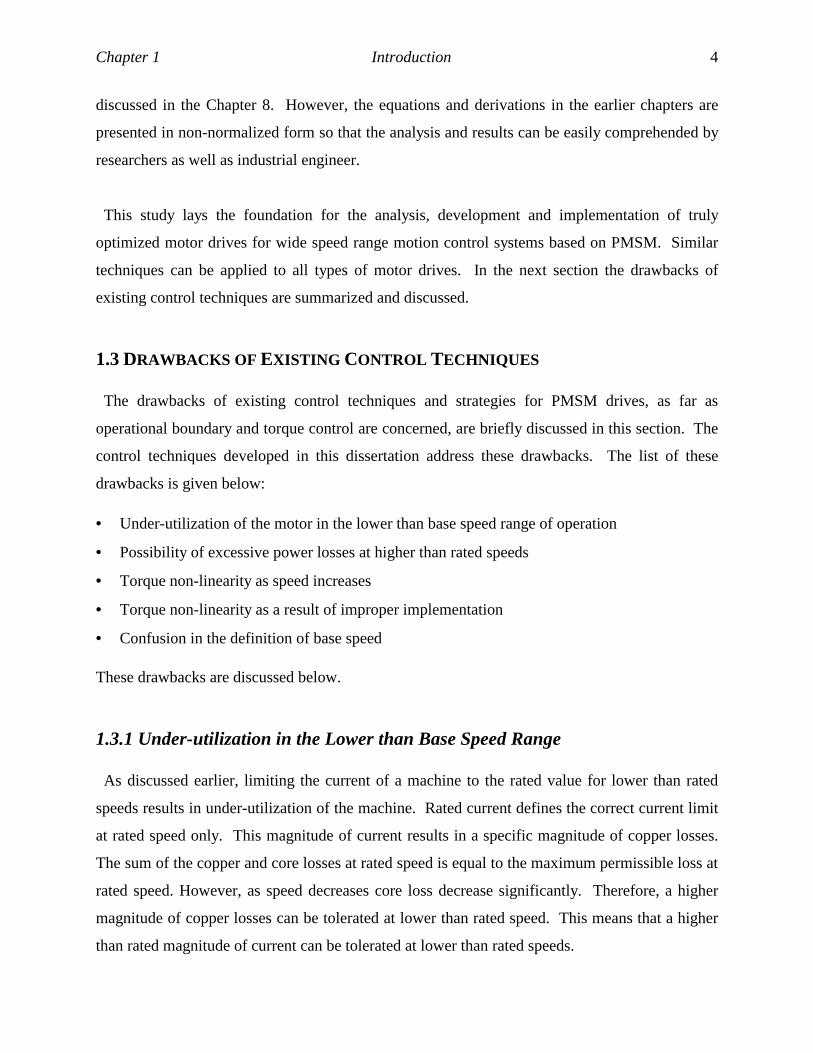
1.3.1 Under-utilization in the Lower than Base Speed Range
As discussed earlier, limiting the current of a machine to the rated value for lower than rated
speeds results in under-utilization of the machine. Rated current defines the correct current limit
at rated speed only. This magnitude of current results in a specific magnitude of copper losses.
The sum of the copper and core losses at rated speed is equal to the maximum permissible loss at
rated speed. However, as speed decreases core loss decrease significantly. Therefore, a higher
magnitude of copper losses can be tolerated at lower than rated speed. This means that a higher
than rated magnitude of current can be tolerated at lower than rated speeds.

Chapter 1 Introduction 5
1.3.2 Excessive Power Losses in the Flux Weakening Range
It is common to limit a machine's power to its rated value in the flux weakening range.
However, limiting the power of the machine to its rated value does not guarantee that the power
losses remain limited. This is due to the fact that core losses increase significantly at higher than
rated speeds. It is shown in Chapter 3 that the net loss can exceed the maximum permissible loss
at a certain speed above rated speed despite the fact that power is maintained at rated level.
1.3.3 Torque Non-linearity Caused by Ignoring Core Losses
Another drawback of most existing control strategies is that they rely on an electrical model of
the machine that does not account for core losses. As speed increases a larger percentage of the
input current is utilized in the generation of core losses. Obviously, this fraction of the input
current does not contribute to the generation of torque. Therefore, the assumption that the entire
input current generates torque at all speeds results in torque non-linearity as speed approaches
the rated speed and beyond.
It is important to realize that core losses constitute a significant portion of the net losses at
speeds close to, and higher, than rated speed. Therefore, any model-based high performance
control strategy must use a model that takes core losses into account. This is specially true if the
system requires linear control of torque at higher than base speeds.
1.3.4 Torque Non-linearity Caused by Improper Implementation
Many implementation schemes presented in the literature assume that the magnitude of current
and torque are proportional for PMSM. In these cases, linear control over current is
implemented in the drive, assuming that linear control over torque follows automatically.
However, this assumption is only valid for some types of PMSM such as the surface mount
PMSM. But, strictly speaking, the relationship between torque and current is not linear for
PMSM. This is specially true for inset and interior PMSM.
Chapter 1 Introduction 6
1.3.5 Confusion in the Definition of Base Speed
The base speed of a machine is defined here as the speed after which generation of maximum
torque requires application of maximum voltage. It is common among traditional high
performance control techniques to use the rated speed as the base speed. Using the rated speed
as the transition point to the flux weakening range is proper only for the surface mount PMSM
running in a nominal environment at rated voltage. It is shown in Chapter 5 that the base speed
is a function of maximum permissible power loss, bus voltage, and the choice of control strategy.
Therefore, simply defining the base speed as rated speed results in improper operation of the
motor drive.
1.4 ADVANTAGES OF THE TECHNIQUES PRESENTED IN THIS DISSERTATION
The application of the analysis and schemes provided in this dissertation result in motor drive
systems with the following advantages:
• Faster dynamics and increased productivity
• Cost savings by maximizing machine utilization
• Optimization of the system based on application’s requirements
• Protection of the machine from excessive power losses
• Adaptability of the motor drive to different environment without changing existing design
• Simple and effective linear torque controllers for wide speed range motor drives
The techniques developed in this dissertation result in maximum utilization of a motor drive
under all operational conditions. This means that more torque and power can be derived from
existing motor drives, resulting in faster dynamic response and increased productivity. On the
contrary, if an application does not require more torque then a motor of smaller size and lower
price can be used. In addition, application of the schemes described in this dissertation result in
operation of the machine within the thermal boundaries imposed by the motor structure and
environmental conditions. Generally, the motor drive becomes more adaptable to different
operating conditions.

Chapter 1 Introduction 7
1.5 POTENTIAL IMPACT ON THE RESEARCH COMMUNITY AND INDUSTRY
The analytical procedures and implementation techniques, presented in this dissertation, in
conjunction with existing knowledge base, are expected to have the following impacts on the
research and industrial communities:
• Operational boundary of all types of motor drives will be defined and studied based on the
constant power loss (CPL) concept.
• Drives will be designed to fully utilize an existing motor’s capacity to make the system
adaptable to different environment by utilizing CPL controllers.
• Similar procedures will be applied to the permanent magnet brushless dc, synchronous
reluctance, switched reluctance and other motors. The permanent magnet brushless dc motor
is an immediate beneficiary since it is widely used in low power high performance
applications.
The content of this dissertation and associated papers can be used as reference on the subjects
discussed above.
1.6 DISSERTATION STRUCTURE
Chapter 2 provides a historical account of motor drives as far as this study is concerned. A
comprehensive literature review in related areas is also given. The control and dynamics of the
PMSM drive operating with constant power loss is proposed and analyzed in chapter 3. A
comparison to traditional operational methods is given. The CPL controller for applications with
cyclic loads is discussed in Chapter 4. The performance of different control strategies for wide
speed range operation of PMSM is analyzed and compared under the CPL concept in Chapter 5.
Implementation strategies for the concurrent flux weakening and torque control of PMSM are
introduced and analyzed in chapter 6. Implementation strategies for the concurrent flux
weakening and torque control of PMSM in the presence of parameter variations are introduced in
Chapter 7. A new normalization technique, along with its applications, is presented in Chapter 8.
The conclusions, summary of contributions, and recommendations for future work are provided
in Chapter 9. Appendix I describes the parameters of the PMSM drive prototype that was used
Chapter 1 Introduction 8
to verify key results of this study. Appendix II describes the procedures used in measuring the
various parameters of the PMSM drive described in Appendix I.
The new normalization technique described in Chapter 8 is used in the analysis of system
performance, and in preparing the code for the simulations, presented in this dissertation. This
normalization technique simplifies the analysis and simulation of system performance.
However, unless otherwise noted, all equations and derivations in this dissertation are presented
as non-normalized statements so that both industrial engineers and researchers can benefit
equally. All variables in plots are normalized using rated values for the respective variables to
enhance the overall presentation and also to simplify the process of generalization of the results.
All simulation codes have been prepared using MATLAB.
1.7 SUMMARY OF CONTRIBUTIONS AND LIST OF CO-AUTHORED PAPERS
The key contributions of this dissertation are outlined below:
• Constant power loss based control strategy to obtain the maximum torque vs. speed envelope
• Its comparison to schemes with current and power limits
• An implementation scheme for the proposed CPL controller and its flexibility for
incorporation into existing drives that may have various control scheme realizations in its
torque and flux controllers
• Derivation of maximum torque and power loss command as a function of maximum
permissible power loss, load duty cycle and speed for applications with cyclic loads
• Comparison of maximum possible torque as a function of maximum possible power loss for
different applications with cyclic loads
• Performance evaluation and comparison of control strategies for the full range of operating
speed based on operation with constant power loss and implementation requirements
• Analytical derivation of maximum speed, maximum current requirements of the drive and
maximum current in the flux weakening range based on the constant power loss criteria
• Analytical derivation of the maximum possible torque as a function of mutual flux linkages
• Implementation schemes for the concurrent flux weakening and torque control for PMSM,
and parameter insensitive controllers based on this concept

Chapter 1 Introduction 9
• Introduction of a new normalization technique that simplifies the analysis and simulation of
PMSM drive operation
• Derivation of the maximum torque vs. speed envelopes for the ME, MTPC, ZDAC, CMFL,
UPF, CBE control strategies operating with constant power loss
• Introduction of generalized application characteristics for PMSM drives using the new
normalization technique
• Experimental verification of key results
List of author’s publications relevant to this dissertation:
•••• R. Monajemy and R. Krishnan, “Control and Dynamics of Constant Power Loss Based
Operation of Permanent Magnet Synchronous Motor,” Conference record, IEEE Industrial
Electronics Conference (IECON), Nov. 29-Dec. 3, 1999, pp. 1452-1457.
•••• R. Monajemy and R. Krishnan, “Performance comparison of six-step voltage and constant
back emf control strategies for PMSM,” Conference record, IEEE Industry Applications
Society Annual Meeting, Oct. 1999, pp. 165-172.
•••• R. Monajemy and R. Krishnan, “Concurrent mutual flux and torque control for the
permanent magnet synchronous motor,” Conference record, IEEE Industry Applications
Society Annual Meeting, Oct. 1995, pp. 238-245.
•••• R. Krishnan, R. Monajemy and N. Tripathi, “Neural Control of High Performance Drives:
An Application to the PM Synchronous Motor Drive”, Invited Paper, Conference records,
IEEE Industrial Electronics Conference (IECON), November, 1995, pp. 38-43.
1.8 ASSUMPTIONS
The following assumptions are made so that the fundamentals of this study can be presented
with better clarity.
• All motor-drive parameters are assumed to be constant unless otherwise noted
• Leakage inductances are zero
• Windage and friction are negligible

Chapter 1 Introduction 10
• Net sustainable loss for a machine is assumed to be constant for the full operating range for
simulation and analytical purposes
• A high band-width current controller is utilized in the drive system resulting in negligible
stator current error
• The rated current is defined as the current that generates rated torque under the zero d-axis
current control strategy
• Base speed is the speed after which flux weakening becomes necessary along the CPL
boundary
1.9 CONCLUSIONS
The operational boundary of any motor drive needs to be set and analyzed based on the
maximum permissible power loss vs. speed profile for the given machine. The traditional
method of defining the operational boundary by limiting torque and power to rated values results
in under-utilization of the system and may subject the motor to excessive power losses. The
analysis of the operational boundary of a motor drive based on the concept of constant power
loss is the main topic of this dissertation. An implementation strategy for enforcing the CPL
operational boundary for a motor drive is presented in this dissertation. The performance of all
advanced control strategies for permanent magnet synchronous motors are analyzed and
compared based on operation of the motor under the CPL concept. Implementation strategies for
concurrent flux weakening and torque control for PMSM are presented. Implementation
strategies for concurrent flux weakening and torque control in the presence of parameter
variations are also presented. All simulation and analysis are performed using an innovative
normalization technique that significantly simplifies the research effort. Experimental
verification of the key theoretical claims of this dissertation are provided using a prototype
PMSM drive described in Appendix I.
11
CHAPTER 2
State of the Art
2.1 INTRODUCTION
In this chapter the rationale behind the research presented in this dissertation is provided.
Permanent magnet synchronous motors and drives are put into perspective from a historical point
of view. The ongoing transition from single-speed to variable-speed motor drives is discussed.
The trends behind this transition are studied. This transition has resulted in the need for
revisiting the area of operational boundaries for motor drives. The state of the art in the areas of
computation of power losses, operational boundaries for variable speed motor drives, control
strategies for high performance variable speed motor drives, and parameter insensitive control
strategies for PMSM are given in this chapter. This chapter justifies the need for the research
effort presented in this dissertation.
Section 2.2 provides a brief history of motors with emphasis on the evolution of PMSM drives.
The period from early 1800s to the 1970s is covered. The trends of the last three decades that are
behind the transition from single speed to variable speed drives are discussed in section 2.3. The
rationale behind choosing the PMSM as the immediate beneficiary of this research effort is
discussed in section 2.4. A literature review on the relevant topics of this dissertation is provided
in section 2.5. The conclusions of this chapter are given in section 2.6.
2.2 THE ELECTRIC MOTOR: A HISTORICAL PERSPECTIVE
In this section motors and motor drives are put into perspective from a historical point of view.
The evolution of the PMSM is traced back in time, and the developments that allow high
performance control over synchronous motors are reviewed.
English physicist and chemist Michael Faraday constructed a primitive model of the electric
motor in 1821. This was a dc motor [1]. By the early 1870s the Belgian-born electrical engineer
Zénobe-Théophile Gramme had developed the first commercially viable dc motor. The dc motor

Chapter 2 State of the Art 12
was in wide spread use in street railways, mining and industrial applications by the year 1900. A
book titled “The Electric Motor and its Applications” [2], published in 1887, is an indication of
the widespread interest in the electric motor in those years. In that book the general theoretical
background necessary for understanding dc motor operation is given. Various types of dc
motors, available at that time, along with their numerous applications and control ideas, with
applications in public transportation, are discussed. The concept of controlled delivery of energy
from a dc power source to a motor in order to meet the specific demands of an application is
discussed. The same process is used today in the majority of high performance control systems.
The following paragraph is a quote from [2], Chapter VII, page 99:
“The Use of Storage Batteries with Electric Motors for Street Railways”
In the present chapter we take up a method which, although now looked upon with distrust by
many, may yet prove to be one of the most feasible means for propulsion of railway cars. We
refer to the employment of accumulators, the stored energy of which, conveyed to the motor in
the form of current, sets it in motion, and with it the car. While this mode of propulsion was until
lately in the experimental state, the progress made has been such that a satisfactory solution of
the problem appears to have been reached; indeed the immediate future will see cars propelled
by the energy derived from accumulators, with success, judged from the standpoint both of
convenience and economy. (T.C. Martin and J. Wetzler, 1887)
However, mass production of combustion engines in the early 1900s, and the abundance of
fossil fuels, delayed the use of accumulators in transportation applications until the present time.
Soon, the disadvantages of dc motors, such as excessive wear in the electro-mechanical
commutator, low efficiency, fire hazards due to sparking, limited speed and the extra room
required to house the commutator, became evident. Faraday’s discovery of the concept of
electromagnetic induction in 1831 paved the way towards the invention of induction motors. In
1883 the Serbian-American engineer Nikolai Tesla invented the first alternating-current
induction motor [3]. Tesla’s motor is generally considered to be the prototype of the modern
electric motor. This was the first brushless motor. The synchronous motor, which is also a
brushless motor, was invented by Tesla as well. By the year 1900 the principles of operation of
synchronous and induction motors were well known. But these motors were not widely used at

Chapter 2 State of the Art 13
that time due to the fact that ac power was not yet commercially available. Flexibility of ac
power led to its initial commercial success even though dc power still cost less at that time. AC
power was easier to produce, distribute, and utilize, as compared to dc power. The fierce
competition between ac and dc power was finally resolved in favor of the ac power by 1890. AC
motors have no commutators, and their speed is only limited by the physical constraints of the
motor. These two advantages led to the wide spread utilization of ac motors in motion control
applications in the following decades.
Induction and synchronous motors utilize the same type of stator. But synchronous motors use
a wound dc field or permanent magnet rotor instead of the wire-wound or squirrel cage rotor of
induction motors. Induction motors can generate torque in a wide range of speed. However,
synchronous motors can only generate torque at the synchronous speed. The synchronous speed
depends on the source frequency. Therefore, the first synchronous motors had to run at speeds of
3600, 1800, 900, … RPM for a line frequency of 60 Hz. The speed of synchronous motors has
to first be increased to synchronous speed by means of an auxiliary motor before the motor can
be used. Introduction of the line-start PMSM in the 1950s provided a solution to this problem.
The rotor of line-start PMSM is made of permanent magnet embedded inside a squirrel-cage
winding. Many induction motors utilize squirrel-cage rotors. Induction of current in the squirrel
cage produces torque at zero or higher speeds the same way torque is generated in induction
motors. Therefore, the line-start PMSM can develop torque at zero speed, and run as an
induction motor, until the synchronous speed is reached. Once the rated speed is reached the
rotor is synchronized with the power source, and no more current is induced in the squirrel cage.
After this, the motor runs as a synchronous motor. However, the high cost of line start PMSM
inhibited its wide spread usage. Eventually, a motor drive was used to convert dc power into ac
power with any desired frequency, and to deliver the power to the motor in a controlled manner.
This development allowed the PMSM to be used efficiently at any speed. The introduction of
high performance motor drives has rendered the line start PMSM almost obsolete. Another type
of synchronous motor is the permanent magnet brushless dc motor (BDCM). The rotor of a
BDCM is similar to that of a PMSM. But, its stator is made of concentrated windings. The
distribution of the stator windings of a PMSM is sinusoidal. The developments that have
contributed to the contemporary BDCM can be traced back to the 1960s when dc motors with

Chapter 2 State of the Art 14
permanent magnets began to displace conventional wound field dc motors. The creation of the
rotor field in wound-field dc motors required a separate supply of dc current. This was a major
burden, specially in the case of low power applications where the cost of providing additional
current for the field hindered their commercial use. In the 1960s permanent magnets were
utilized instead of the wound field, which made this motor viable for many servo applications
and other low power motion control systems. However, permanent magnet dc motors still had
the fundamental problems of dc motors mentioned earlier. Eventually, with the advent of
electronic drives, it became possible to place the magnets of the motor on the rotor, and the
windings on the stationary stator. In this case the drive’s primary function is to switch current
into the right phase depending on rotor position. The BDCM motor is also known as the inside-
out dc motor! The BDCM motor does not require a commutator or brushes, since the function of
the brushes is delegated to the drive. Obviously, no sparks are generated because the
commutation of current is not performed mechanically. From a fundamental point of view the
BDCM motor can be considered a special type of PMSM. In both cases the speed of the motor
is proportional to the input current frequency. And, in both cases the magnet is on the rotor and
the winding is on the stator. This makes the cooling of the motor easier as compared to the dc or
induction motor. While the back emf of a PMSM is sinusoidal, the back emf of a BDCM is
trapezoidal. BDCM is usually used for lower performance applications, such as pumps and fans,
and PMSM is mostly used in high performance applications that require high quality torque. It is
only for such applications that the higher cost of a PMSM can be justified.
The torque vs. current relationship for synchronous motor is non-linear. The torque of
synchronous motor depends on both current magnitude and the angle of current phasor with
respect to the rotor. This results in complications as far as control is concerned. Blondel’s study
of synchronous motors [4], 1913, along with Park’s transformation [5], 1933, paved the way
towards linear and instantaneous control over torque for PMSM [6]. Park’s theory presented a
transformation between variables in the stationary and the rotor reference frames which yields
the two-axis equivalent circuit for a PMSM. From the rotor’s point of view every variable has a
magnitude and angle which is constant in steady state. This means that using equations and
variables in the rotor reference frame makes the analysis and control of PMSM much easier.
Essentially, Park introduced auxiliary variables in terms of which the machine equations become

Chapter 2 State of the Art 15
much simpler. Availability of this transformation led to a field referred to as “vector control.”
Vector control enables independent control over the magnitude and angle of current with respect
to the rotor such that instantaneous control over torque is possible. Application of vector control
to a PMSM allows for linear control over torque, as well as control over different performance
criteria such as efficiency and power factor.
Several trends, starting in the 1970s, created a demand for high performance variable speed
motor drives. The trends that are directly relevant to this research effort are discussed next.
2.3 TRENDS FORCING THE TRANSITION TO VARIABLE SPEED DRIVES
The sudden rise in the cost of energy in the 1970s, recent trends towards conservation of the
environment, and the requirements of new applications, have created a significant demand for
variable speed drives. The transition from single speed drives to variable speed drives has left
some areas open for research. These areas include the operational boundary of motor drives and
high performance control strategies for wide speed range motor drives. The issues that deserve
further research in these areas are discussed here in light of the relevant trends during the last
three decades.
Low energy costs in the 1950-70 era resulted in the wide spread use of several types of motors
without regard to efficiency or other performance criteria. However, increasing energy costs in
that last 30 years, public concern over unnecessary use of power and environmental concerns are
driving manufactures to develop more efficient motion control systems. It is estimated that 10%
of all electrical energy is wasted since many motors that do not have drives run at idle for long
periods of time. A much higher percentage of energy is lost simply due to the low efficiency of
many motion control systems. Fans, blowers and pumps represent 50% of all drive capacity
today. These applications can benefit significantly from being able to operate at optimal speed
using a drive. Power consumption increases exponentially with speed. Therefore, running
continuously at a lower optimal speed is better than running in the on-off mode at a higher speed.
Most of today’s fans, blowers and pumps still operate in the on-off mode. Also, on-off operation
wears off the motor faster, and therefore, motors with drives can have a longer life. Drives help
ameliorate transients during startup of motors. Motors without drives draw significant

Chapter 2 State of the Art 16
magnitudes of current during startup and during transient operation. Drives solve this problem
elegantly. Variable speed drives can increase system efficiency by 15 to 27 percent [7]. Many
applications, such as the hybrid vehicle and machine tools, require variable speed operation to
begin with. On the other hand several energy acts, such as the energy act of 1992, impose
minimum efficiency on motors and drives. These trends justify the rapid deployment of drives in
many motion control applications. It is estimated that the capital costs of adding drives to
motors are paid pack in relatively short periods of time due to the savings in energy costs.
All of the issues discussed above have resulted in a significant movement towards the
utilization of variable speed drives instead of single speed systems for many motion control
applications. However, while this transition is in progress, some of the control methods of single
speed systems have been inadvertently carried over to new systems. The operational boundary
of variable speed motor drives are being defined by rated current and power of the machine.
But, these limitations are only valid at rated speed. The consequences, as studied in this
dissertation, are under-utilization of the motor as well as placing the motor at risk of excessive
power losses. This is true for all major classes of motors, i.e. induction motors, BDCM and
PMSM, that are now being utilized in most variable speed applications. Some of the torque
control strategies that are applied to existing advanced PMSM drives are, in fact, carried over
from dc motors. For example, in many cases it is assumed that torque and current are
proportional. Therefore, the torque control strategy is usually based on the assumption that the
relationship between current and torque is linear. However, for several types of PMSM, such as
the inset and interior PMSM, current and torque are not proportional. Some researchers have
presented linear torque control techniques that can be applied to all types of PMSM [8, 9]. The
definition of base speed, generally assumed to be the rated speed of the motor, is another area
where clarification is required. The base speed of a motor is defined here as the speed after
which generation of maximum torque requires application of maximum voltage. In particular the
base speed for interior PMSM is significantly influenced by control strategy, maximum available
voltage, and maximum permissible power loss as later shown in Chapter 5. The theoretical
analysis and implementation strategies presented in this dissertation address the above issues.

Chapter 2 State of the Art 17
2.4 WHY CONCENTRATE THIS STUDY ON PMSM?
While the transition from single speed to variable speed systems is in progress, another
transition is in effect within the field of variable speed motor drives. Direct current and
induction motor drives, which have dominated the field until now, are being replaced by PMSM
and BDCM drives for low power applications. Low power is defined here as being less than 10
kW. Some of the applications for motors below 10 kW are in home appliances, electric tools and
small pumps and fans. PMSM and BDCM have the following advantages over dc motors:
• less audible noise
• longer life
• sparkless (no fire hazard)
• higher speed
• higher power density and smaller size
• better heat transfer
PMSM and BDCM have the following advantages over induction motors:
• higher efficiency
• higher power factor
• higher power density for lower than 10 kW applications, resulting in smaller size
• better heat transfer
The above comparison shows that the PMSM and BDCM are superior to the induction motor for
low power applications. The operation of the BDCM and the PMSM is very similar from a
fundamental point of view. Therefore, all the analysis and control strategies developed for the
PMSM readily applies to the BDCM. The above discussion justifies the choice made in this
dissertation. The same techniques developed in this dissertation can be applied to all high
performance motor drives.
2.5 LITERATURE REVIEW
The state of the art in the following areas is discussed in this section:

Chapter 2 State of the Art 18
• Power losses and efficiency
• Operational boundaries of motor drives
• Control strategies for operation below base speed
• Control strategies for operation above base speed
• Parameter sensitivity and parameter insensitive control strategies
2.5.1 Power Losses and Efficiency
The temperature of a machine rises as a function of power losses in the machine, and machines
have operational limits as far as temperature is concerned. Therefore, the operational boundary
of a motor drive depends on how much loss can be tolerated. The main sources of losses are
copper and core losses. Friction and windage also result in losses. The study of losses and
efficiency are closely related since lower losses at the same torque and speed result in a more
efficient machine. Motors with higher efficiency can be relatively smaller. In other words,
higher efficiency directly translates into higher power density. Efficiency at reduced speed is
critical due to the fact that many drives run at 40% to 80% of rated speed most of the time.
The efficiency and power density of PMSM have been studied by several researchers [10, 11,
12]. [10] gives solid comparison results showing that permanent magnet brushless motors
provide higher efficiency, higher power factor and higher power density for lower than 7 kW
applications as compared to induction motors. [11] gives a comparison between the PMSM and
induction motor showing that the product of efficiency and power factor for PMSM is 30% to
40% higher as compared to induction motor in the lower than 7 kW power range. The higher
efficiency of the PMSM translates into lower losses for same power output as compared to
induction motors. Therefore, the size of a PMSM is smaller than an induction motor capable of
delivering the same power. This results in higher power density for PMSM. [12] shows that the
power density of the BDCM is higher than that of the PMSM.
Copper and core losses are the most fundamental and dominant losses in PMSM. Copper losses
are proportional to the square of current. Core losses have been studied by several researchers
[13, 14, 15]. The main sources of core losses are Eddy currents and hysteresis losses. The
induction of current inside the stator core causes Eddy current losses. Hysteresis losses are the

Chapter 2 State of the Art 19
result of continuous variation of flux linkages in the core. Eddy current losses are nearly
proportional to the square of the product of air gap flux linkages and frequency of the flux
variation. Hysteresis losses are nearly proportional to the product of square of flux linkages and
frequency of flux variation. Several research papers [10, 13, 16] have reported net core losses
that are between 20% to 30% of total loss at rated speed and torque for PMSM below 7 kW.
Core losses are obviously negligible at very low speeds. However, as speed increases the share
of power losses due to core losses increases significantly. Several researchers [17, 18, 19, 20,
21, 22] have utilized an electrical model of PMSM that includes a parallel resistance that
accounts for core losses in high performance applications. [19, 20, 21, 22] deal with efficiency
of the synchronous reluctance motor. It can be concluded from the above discussion that both
copper and core losses need to be accounted for in the analysis and control of high performance
of motor drives.
Another portion of losses is due to stray losses. Stray losses are the result of distortion of the
air gap flux by the phase current [23]. Non-uniform distribution of current in the copper also
leads to stray losses [23]. Stray losses are very difficult to estimate. Therefore, these losses are
usually bundled with core losses during modeling or during experimental measurements.
2.5.2 Operational Boundaries of Motor Drives
The number of research papers that directly investigate the subject of operational limits of
PMSM motor drives for variable speed applications is very limited [16, 24, 25, 26, 28]. [25,26]
deal with choosing motor parameters such that the motor is suitable for a given maximum speed
vs. torque envelop. [24, 25] investigate the optimal design of a motor for delivering constant
power in the flux weakening range. Operating limits of PMSM are studied in [27, 28] based on
the constant power criterion. All papers on high performance control of PMSM define the
operational boundaries of any control strategy by limiting current and power to rated values for
the full range of operating speed.
2.5.3 Control Strategies for Operation Below Base Speed
In the lower than base speed operating range one performance criteria can be optimized while
torque linearity is being maintained at the same time. This degree of freedom can be utilized in

Chapter 2 State of the Art 20
implementing different control strategies. The main control strategies for PMSM for the lower
than base speed operating range are:
(a) Zero d-axis current (ZDAC)
(b) Maximum torque per unit current (MTPC)
(c) Maximum efficiency (ME)
(d) Unity power factor (UPF)
(e) Constant mutual flux linkages (CMFL)
The ZDAC control strategy [29, 30] is widely used in the industry as it forces the torque to be
proportional to current magnitude for the PMSM. The basics behind the MTPC control strategy
have been known for several decades. This control strategy was made popular recently by [31].
The MTPC control strategy [31] provides maximum torque for a given current. This, in turn,
minimizes copper losses for a given torque. The MTPC control strategy is utilized in high
performance applications where efficiency is important, and is the one most studied and utilized
control strategy by PMSM motor drive researchers. However, the MTPC control strategy does
not optimize the system for net loss. The UPF control strategy [29] optimizes the system’s Volt-
Ampere requirement by maintaining the power factor at unity. The ME control strategy [17, 18]
minimizes the net loss of the motor at any operating point. This control strategy is particularly
appealing in battery operated motion control systems in order to extend the life of the system.
The CMFL control strategy [29] limits the air gap flux linkages to a known value which is
usually the magnet flux linkages. This is to avoid saturation of the core.
Each of the above mentioned control strategies have their own merits and demerits. [29]
provides a comparison between the ZDAC, UPF and CMFL control strategies from the point of
view of torque per unit current ratio and power factor. The UPF control strategy is shown to
yield a very low torque per unit current ratio. The ZDAC control strategy results in the lowest
power factor among the five control strategies. [32] provides a comparison between the MTPC
and ZDAC for an interior PMSM. This study shows that the MTPC control strategy is superior
in both efficiency and torque per unit current as compared to the ZDAC control strategy. Torque
is limited to rated value in all existing control techniques for the lower than base speed operating
range. This operating range is referred to as the constant torque operating range. It is shown in

Chapter 2 State of the Art 21
Chapter 3 that the maximum torque in the lower than base speed operating range is not a
constant. A thorough comparison of all five control strategies from the point of view of
maximum torque vs. speed profile, power losses, efficiency, torque per unit current, power
factor, voltage requirements and implementation complexity has not been published. Such a
comparison is made in this dissertation in order to provide a sound basis for choosing the optimal
control strategy for a particular motor drive application.
2.5.4 Control Strategies for Operation above Base Speed
The fundamental component of voltage applied to each phase must remain constant in the
higher than base speed operating range. Performance criteria other than torque linearity cannot
be enforced in this range due to the fact that a restriction on voltage is imposed. This range of
operation is also referred to as the flux weakening range. Two control strategies are possible
depending on whether maximum phase voltage is applied or the phase voltage is limited to a
level lower than maximum possible. These control strategies are:
(a) Constant back emf (CBE)
(b) Six-step voltage (SSV)
The CBE control strategy [8, 27, 33] limits the back emf to a value that is lower than the
maximum possible voltage to the phase. By doing this, a voltage margin is retained that can be
used to implement instantaneous control over phase current. Applications that require high
quality of control over torque in the higher than base speed operating range utilize the CBE
control strategy. The SSV control strategy applies maximum possible voltage to the phase. In
this case only the average torque can be controlled, and a relatively higher magnitude of torque
ripple is present. A procedure for studying the performance of an induction motor under the
SSV control strategy is presented in [34]. Performance evaluation of the SSV control strategy
has been presented for BDCM [35, 36].
References [8, 27, 33, 37, 38] provide insight into the high performance control of PMSM in
the flux weakening range. The topics discussed include linear torque control schemes, speed
range, implementation strategies and torque vs. speed profile. The power is limited to rated
Chapter 2 State of the Art 22
power in all these studies. Therefore, this range of operation is also referred to as the constant-
power operating range. It is later shown in this dissertation that maximum power of a motor is
not a constant in variable speed applications operating above base speed. Most of the control
strategies for the flux weakening range of PMSM result is non-linear control over torque. This
happens either because of neglecting the impact of core losses or by erroneous implementation
strategies. The SSV control strategy is widely utilized in many applications [39]. However, a
comprehensive study of the pros and cons of this control strategy has not been performed.
Ref. [38] provides an implementation scheme for a wide speed range controller for a PMSM.
The transition to flux weakening range is implemented by comparing an estimation of phase
voltage with the maximum available voltage, the latter being itself a measured variable.
Therefore, the transition to flux weakening range happens in an orderly fashion even if the bus
voltage varies. The output of the speed proportional-integrator (PI) controller commands the
magnitude of current to be enforced on each phase. The relationship between current and torque
is not linear in inset and interior PMSM. Therefore, the current command vs. torque gain
changes depending on the magnitude of torque in the above mentioned implementation scheme.
This complicates the design of the speed PI controller. Strictly speaking, the best strategy is to
let the output of the speed PI controller control torque directly so that the speed PI controller can
be designed based on the constant gain relating the torque command to the actual torque.
2.5.5 Parameter Sensitivity and Parameter Insensitive Control Strategies
All high performance control strategies for PMSM are based on an electrical model of the
machine. In most cases, the parameters of the machine are assumed to be constant. In reality
machine parameters vary as a function of temperature and current. Phase resistance of a motor
varies with temperature and frequency. An increase of as much as 100% is possible with a
100 Co rise in temperature. The inductance of some types of PMSM vary by as much as 20% of
the rated value. This is specially true for the interior PMSM [40]. The inductance is a function
of current. The nonlinear magnetic properties of the core are the reason behind the variations of
inductance as a function of current. The magnet’s flux density changes as a function of
temperature [41]. A reduction of 20% is possible for a 100 Co rise in the temperature of the
magnet. If the temperature rises beyond a certain level the magnet may permanently loose part

Chapter 2 State of the Art 23
of its flux density. This temperature threshold depends on the particular characteristics of the
magnets. Another parameter that varies in some applications is the dc bus voltage input to the
drive. The variation of the dc bus voltage affects the speed after which flux weakening must be
initiated. Also, the maximum torque in the flux weakening range and the maximum possible
speed both depend on the dc voltage input value. Inductance can be estimated if the inductance
vs. current relationship is accurately known. Bus voltage can be monitored at all times.
Resistance can be estimated by measuring the temperature of the core. The variations of the
magnet flux density can be estimated if the temperature of the magnet is measured. However,
this is a difficult and costly process due to the fact that the rotor is not stationary. An on-line
estimation of these parameters can be incorporated in the model being used to control the
machine. Core losses also impact the model of a PMSM. Failure to account for core losses
results in torque non-linearity.
Ref. [40] provides an example of a high performance PMSM drive where the phase inductance
in the electrical model is a function of current. Ref. [20] has studied vector control of a
synchronous reluctance motor including inductance variations. Ref. [41] evaluates the impact of
temperature on efficiency and torque of a PMSM. References [42] and [43] present parameter
insensitive control strategies that yield speed and torque linearity, respectively, in the presence of
magnet flux linkages variations.
2.6 CONCLUSIONS
A historical account of motor drives with emphasis on PMSM drives is given in this chapter.
The evolution of permanent magnet synchronous motors and motor drives is studied. The
transition from single speed to variable speed control system is emphasized. It is shown that
some areas, such as the operational envelope, evaluation and comparison of control strategies,
and implementation techniques for wide speed range control strategies, need to be further
investigated. The analytical procedures and implementation schemes provided in this
dissertation are applicable to all motor drives, and can be used to optimize any motion control
system. However, it is shown that the PMSM drive is the most likely beneficiary of the different
concepts introduced in this dissertation. The state of the art in the areas of computation of power
losses and efficiency, operational boundaries, high performance control strategies, and parameter
insensitive control strategies for PMSM, is given.
24
CHAPTER 3
Control and Dynamics of Constant Power Loss Based
Operation of Permanent Magnet Synchronous
Motor Drive System
3.1 INTRODUCTION
The operational boundary of an electrical machine is limited by the maximum permissible
power loss for the machine. The control and dynamics of the PMSM drive operating with
constant power loss are proposed in this chapter. The proposed operational strategy is modeled
and analyzed. Its comparison to other control strategies that limit current and power to rated
values demonstrates the superiority of the proposed scheme. The implementation of the proposed
scheme is developed. This has the advantage of retrofitting the present PMSM drives with least
amount of software/hardware effort. The PMSM drives in this case then can use the existing
controllers to implement any control criteria such as the ones described earlier in sections 2.5.3
and 2.5.4. Experimental verification of the proposed constant power loss operational strategy is
provided.
The maximum torque vs. speed envelope for the control strategies in the lower than base speed
range is commonly found by limiting the stator current magnitude to the rated value. In the
higher than base speed range the shaft power is commonly limited to rated value. Current
limiting restricts copper losses but not necessarily the core losses. Similarly, limiting the shaft
power does not limit power losses directly. Limiting current and power to rated values ignores
the thermal robustness of the machine that requires the total loss be constrained to a permissible
value. Rated current and power guarantee acceptable power loss only at rated speed. Therefore,
these simplistic restrictions are only valid for motion control applications requiring operation at
rated speed. Increasingly at present single speed motion control applications are being retrofitted
Chapter 3 Control and Dynamics of CPL Based Operation of PMSM Motor Drive 25
or replaced with variable speed motor drives to increase process efficiency and operational
flexibility. Also for manufacturing cost optimization, the same machine designs are utilized in
vastly different environmental conditions thus necessitating control methods to maintain the
thermal robustness of the machine while extracting the maximum torque over a wide speed
range. The constant power loss (CPL) based operation provides the maximum torque vs. speed
envelope from these viewpoints, and such a scheme is proposed in this chapter. A comparison of
this operational boundary and the operational boundary resulting from limiting current and power
to rated values is presented. This comparison clearly reveals that the proposed method results in
a significant increase in permissible torque at lower than rated speeds. Consequently, the
dynamic response is enhanced below the base speed. It is also demonstrated that the
conventional method of limiting current and power to rated values can lead to the generation of
excessive power losses in the flux weakening range.
An implementation strategy for the proposed scheme is developed. This implementation
strategy is based on an outer power loss feedback control loop. The input to the system is the
desired maximum power loss of the machine. The feedback loop limits the torque command
such that the power loss does not exceed the maximum set value at any operating point. This
system is applicable to all types of motor drives for the full range of operation, and is
independent of the choice of control strategy for dynamic control of torque. The proposed
implementation strategy can be integrated into all high performance motor drives with very little
modification in their control algorithms. Real-time estimations of machine parameters can also
be utilized as extra inputs to this implementation strategy. Experimental results from a laboratory
prototype are included to verify the proposed implementation to enforce the maximum torque vs.
speed envelope in a torque controlled PMSM drive system. Load duty cycle can be integrated in
maintaining the effective total power loss by varying the power loss reference in the outer control
loop as a function of load duty cycle. Issues concerning load duty cycle are dealt with in Chapter
4. Further it is noted that the underlying control algorithm lends itself to real-time
implementation. The maximum permissible power loss of a machine must be chosen based on a
preset temperature rise for the machine. Therefore, the permissible constant power loss may vary
significantly depending on the operational environment, ambient temperature and the cooling
arrangement for the machine.

Chapter 3 Control and Dynamics of CPL Based Operation of PMSM Motor Drive 26
All derivations and examples given in this chapter apply to the PMSM. This choice is made
since the PMSM is regularly utilized in high performance applications and can benefit
significantly from the proposed constant power loss controller (CPLC). A similar approach can
be applied to other types of machines with minor modifications.
The contributions of this chapter are summarized below:
• A constant power loss based control strategy to obtain the maximum torque vs. speed
envelope
• Its comparison to schemes with current and power limits
• An implementation scheme for the proposed CPLC and its flexibility for incorporation in
existing drives that may have various control scheme realizations in its torque and flux
controllers
The CPLC scheme for PMSM is studied using a PMSM model given in section 3.2. The
analysis of the CPLC scheme and its comparison to the control schemes limiting the current and
power to rated values, is presented in section 3.3. The current rating of the drive and parameter
sensitivity of the CPLC scheme are discussed in section 3.4. The implementation strategy for the
CPLC is presented in section 3.5. Experimental correlation is provided in section 3.6.
Techniques for using the power loss command to control the drive are discussed in section 3.7.
The conclusions of this study are summarized in section 3.8. The equations that describe the
constant power loss operational envelope are omitted from this chapter for the sake of clarity.
These equations are provided in Chapter 8 in normalized format.
3.2 PMSM MODEL WITH LOSSES
A dq model for a PMSM in rotor reference frame in steady state with simplified loss
representation is given in Fig. 3.1, where, qsI and dsI are q and d axis stator currents,
respectively, and qsV and dsV are q and d axis stator voltages, respectively. qI and dI are q
and d axis torque generating currents, respectively, and qcI and dcI are q and d axis core loss
currents, respectively. sR and cR are stator and core loss resistors, respectively, and qL and
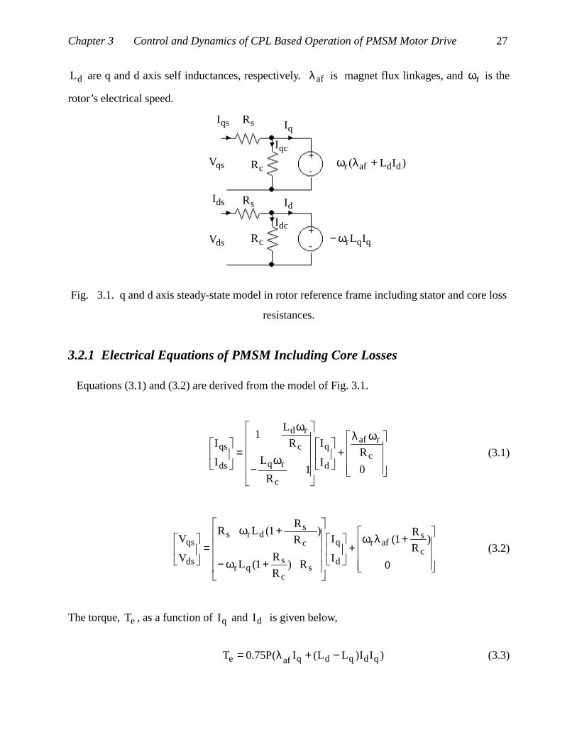
Chapter 3 Control and Dynamics of CPL Based Operation of PMSM Motor Drive 27
dL are q and d axis self inductances, respectively. afλ is magnet flux linkages, and rω is the
rotor’s electrical speed.
qsV
dsV
)IL( ddafr +λω
qqr ILω−
qsI
dsI
qI
dI
qcI
dcI
sR
sR
cR
cR
Fig. 3.1. q and d axis steady-state model in rotor reference frame including stator and core loss
resistances.
3.2.1 Electrical Equations of PMSM Including Core Losses
Equations (3.1) and (3.2) are derived from the model of Fig. 3.1.
ωλ+
ω−
ω
=
0
RI
I
1R
L
R
L1
I
Ic
raf
d
q
c
rq
c
rd
ds
qs(3.1)
+λω+
+ω−
+ω=
0
)R
R1(
I
I
R)R
R1(L
)R
R1(LR
V
Vc
safr
d
q
sc
sqr
c
sdrs
ds
qs(3.2)
The torque, eT , as a function of qI and dI is given below,
)II)LL(I(P75.0T qdqdqafe −+λ= (3.3)

Chapter 3 Control and Dynamics of CPL Based Operation of PMSM Motor Drive 28
where eT is torque, and P is the number of rotor poles.
3.2.2 Total Power Loss Equation for PMSM
The net core loss, lcP , for the machine is computed as follows:
c
2ddaf
2r
c
2qq
2r
lc R
)IL(5.1
R
)IL(5.1P
+λω+ω
= 2m
2r
cR
5.1 λω= (3.4)
where mλ is the air gap flux linkages. Note that in practice a more complex representation of
core losses, based on elaborate equations or tables, can be used to increase the accuracy of the
core loss estimation at higher speeds.
The total machine power loss, lP , including both copper and core losses, can be described as,
])IL()IL[(R
5.1)II(R5.1P 2
ddaf2
qq2r
c
2ds
2qssl +λ+ω++= (3.5)
Another major source of power losses is the electronic inverter. However, inverter losses do not
impact the operational envelope of the machine. This is due to the fact that the cooling
arrangement for the inverter is separate from the cooling arrangement for the machine.
Therefore, inverter losses are not considered in this dissertation. Inverters limit the maximum
current and voltage that can be delivered to a machine. It is presumed that the operating
envelope of the inverter satisfies the motor operation.
In the next section the operational envelope resulting from the application of the CPLC to a
PMSM is discussed.
3.3 CONSTANT POWER LOSS CONTROL SCHEME AND COMPARISON
The maximum permissible power loss, lmP , depends on the desired temperature rise for the
machine. lmP can be chosen to be equal to the net loss at rated torque and speed assuming that
Chapter 3 Control and Dynamics of CPL Based Operation of PMSM Motor Drive 29
the machine is running under exact operating conditions defined in manufacturer data sheets. At
any given speed the current phasor, which is the resultant of qI and dI , and its trajectory for
maximum power loss is given by (3.5) with lP replaced by lmP . This trajectory is a circle at zero
speed, and a semi-circle at non-zero speeds. The operating point of a PMSM must always be on
or inside the trajectory defined by (3.5) for that speed so that the net loss does not exceed lmP .
At any given speed the operating point on the constant power loss trajectory which also results in
maximum torque defines the operational boundary at that speed. At this operating point,
maximum torque is generated for the given power loss of lmP . To find the maximum
permissible torque at a given speed it is sufficient to move along the trajectory defined by (3.5)
for a given lmP and find the operating point that maximizes (3.3). In the flux weakening range,
both voltage and power loss restrictions limit the maximum torque at any given speed. The
following relationship is true for any stator current phasor operating point in the flux weakening
range assuming that the voltage drop across the phase resistance is negligible,
mrr5.02
ddaf2
qqsm ])IL()IL[(V λω=ω+λ+= (3.6)
where smV is either the maximum desired back emf or the fundamental component of maximum
voltage available to the phase. The latter applies to the six step voltage control strategy. At any
given speed in the flux weakening range the stator current phasor that results in a set power loss
can be found by solving equations (3.5) and (3.6). This operating point corresponds to the
maximum permissible torque at the given speed in the flux weakening range. Fig. 3.2 shows the
maximum torque possible for the full range of speed for the motor drive described in Appendix I.
All variables in Fig. 3.2 are normalized using rated values. The power loss is limited to the rated
value of 121 Watts at all operating points. The following assumption is used in solving the
required equations as discussed above,
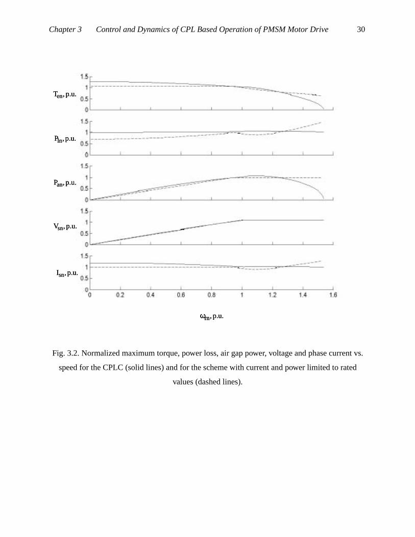
Chapter 3 Control and Dynamics of CPL Based Operation of PMSM Motor Drive 30
Fig. 3.2. Normalized maximum torque, power loss, air gap power, voltage and phase current vs.
speed for the CPLC (solid lines) and for the scheme with current and power limited to rated
values (dashed lines).
p.u.,Ten
p.u.,Pln
p.u.,Pan
p.u.,Vsn
p.u.,Isn
p.u.,rnω
p.u.,Ten
p.u.,Pln
p.u.,Pan
p.u.,Vsn
p.u.,Isn
p.u.,rnω
p.u.,Ten
p.u.,Pln
p.u.,Pan
p.u.,Vsn
p.u.,Isn
p.u.,rnω
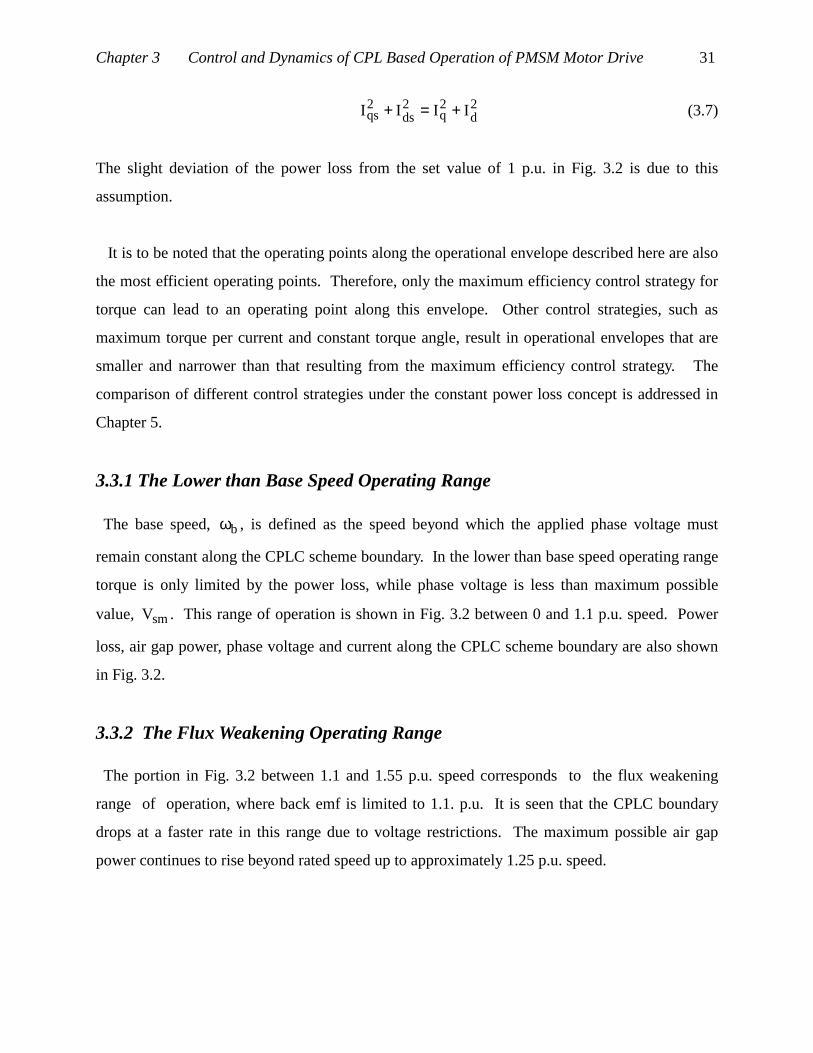
Chapter 3 Control and Dynamics of CPL Based Operation of PMSM Motor Drive 31
2d
2q
2ds
2qs IIII +=+ (3.7)
The slight deviation of the power loss from the set value of 1 p.u. in Fig. 3.2 is due to this
assumption.
It is to be noted that the operating points along the operational envelope described here are also
the most efficient operating points. Therefore, only the maximum efficiency control strategy for
torque can lead to an operating point along this envelope. Other control strategies, such as
maximum torque per current and constant torque angle, result in operational envelopes that are
smaller and narrower than that resulting from the maximum efficiency control strategy. The
comparison of different control strategies under the constant power loss concept is addressed in
Chapter 5.
3.3.1 The Lower than Base Speed Operating Range
The base speed, bω , is defined as the speed beyond which the applied phase voltage must
remain constant along the CPLC scheme boundary. In the lower than base speed operating range
torque is only limited by the power loss, while phase voltage is less than maximum possible
value, smV . This range of operation is shown in Fig. 3.2 between 0 and 1.1 p.u. speed. Power
loss, air gap power, phase voltage and current along the CPLC scheme boundary are also shown
in Fig. 3.2.
3.3.2 The Flux Weakening Operating Range
The portion in Fig. 3.2 between 1.1 and 1.55 p.u. speed corresponds to the flux weakening
range of operation, where back emf is limited to 1.1. p.u. It is seen that the CPLC boundary
drops at a faster rate in this range due to voltage restrictions. The maximum possible air gap
power continues to rise beyond rated speed up to approximately 1.25 p.u. speed.

Chapter 3 Control and Dynamics of CPL Based Operation of PMSM Motor Drive 32
The operational boundary resulting from limiting current and power to rated values is also
shown in Fig. 3.2. It can be concluded from the example that the application of the constant
current and power operational envelope results in:
• Under-utilization of the machine at lower than base speed
• Generation of excessive power losses at higher than rated speeds unless both power and
current are limited to rated values in the flux weakening range
• Under-utilization of the machine in some intervals of the flux weakening range
3.4 SECONDRY ISSUES OF THE CPL CONTROLLER
3.4.1 Higher Current Requirement at Lower than Base Speed
It is seen from Fig. 3.2 that the CPLC provides 39% higher torque at zero speed as compared to
the maximum torque possible with rated current. This requires 36% more than rated current at
zero speed or in the very low speed operating range. It is to be noted that this additional current
requirement does not result in a proportional increase in the price of the drive. This is mainly
due to the fact that the voltage requirements of both control strategies are similar as seen from
Fig. 3.2. Therefore, the power switches have to be upgraded only for current and not for higher
voltage.
3.4.2 Parameter Dependency
The CPLC scheme is dependent on machine parameters dL , qL , afλ , cR and sR . The d-axis
path of the rotor involves a relatively large effective air gap, and does not saturate under normal
operating conditions. Therefore, dL does not vary significantly. qL varies as a result of
magnetic saturation along the q-axis, and can be estimated accurately as a function of phase
current [40]. An accurate estimation of afλ requires more complex algorithms [43]. sR varies
as a function of temperature. Any implementation strategy for the CPLC is by nature parameter-
dependent. This is the case with all model-based control strategies.

Chapter 3 Control and Dynamics of CPL Based Operation of PMSM Motor Drive 33
Motor
mθ
*eT
~
mω
+
_
Wide speed-range lineartorque controller
Resolver &Tachometer
*qsi
*dsi
Current controllerand power stage
Power lossestimator
*eT
+ _*lP
limT
mω
lP
Peaktorquelimiter
PI Controller Filter
PI
*rω
mω
lfP
Fig. 3.3. Implementation scheme for the constant power loss controller.
3.5 IMPLEMENTATION SCHEME FOR THE CPL CONTROLLER
Fig. 3.3 shows the block diagram for an implementation strategy of the CPLC scheme. The
wide speed-range linear torque controller is assumed to provide torque linearity over the full
range of operating speed including the flux weakening range. Any control strategy can be
utilized in the torque controller block. The copper and core losses of the machine are estimated
using (3.5) utilizing the q and d axis current commands, *qsi and *
dsi , as well as measured speed,
mω . All the required variables for power loss estimation are already available within most high
performance control systems. The estimated net power loss, lP , is always a positive number as
seen from (3.5). lfP is the filtered version of lP . The filtered power loss estimation is
compared with the power loss reference, *lP . The difference is processed through a proportional
and integrator (PI) controller. The output of the power loss controller determines the maximum
permissible torque, limT . The torque command, *eT , is the output of a PI controller operating on
the difference of the commanded and measured speeds. If the torque command is higher than
limT then the system automatically adjusts the torque to the maximum possible value, limT .

Chapter 3 Control and Dynamics of CPL Based Operation of PMSM Motor Drive 34
However, if the torque command is less than the maximum possible torque at a given speed then
the torque limit is set at absolute maximum value leaving the torque command unaltered. The
same absolute value of the torque limit is applied to both positive and negative torque
commands. The magnitude of transient torque is limited by the peak torque limiter block. The
processed torque command, *eT
~, and mω , are inputs to the wide speed range linear torque
controller. The outputs of this block are *qsi and *
dsi . The current controller and power stage
enforce the desired current magnitude and its phase on the motor. The inputs to this stage are
*qsi , *
dsi , and rotor position, mθ .
The salient features of the CPL controller are summarized below:
• Off-line calculation of the maximum torque vs. speed envelope is not necessary
• Maximum power loss can be adjusted by an operator or by process demand
• An on-line estimation of qL , afλ and sR can be used by the power loss estimation block to
increase accuracy
• The system is independent of the control strategy used in the linear torque controller block
• All necessary parameters are already available in most high performance controllers
• The scheme lends itself to real-time implementation
3.6 EXPERIMENTAL CORRELATION
Experimental correlation is provided using a prototype motor drive utilizing an interior PMSM
with parameters given in Appendix I. The experimental PMSM motor drive is set up as a torque
controller for lower than base speed operating range. The power loss controller is implemented
as shown in Fig. 3.3. The functions required in estimating the machine power losses are
implemented using 8 bit multiplying DACs. The maximum efficiency control strategy is
implemented for the dynamic control of torque. This requires that the q and d-axis currents be
functions of both measured speed and torque commands. Two 8 kByte EEPROM lookup tables
are utilized in this process. The maximum set power loss is 30 W. Fig. 3.4 shows the maximum

Chapter 3 Control and Dynamics of CPL Based Operation of PMSM Motor Drive 35
possible measured torque and current, predicted maximum torque, as well as corresponding core,
copper and net losses vs. speed. The torque command is set at the maximum value of 1.5 N.m.
It is seen that as speed increases the maximum possible torque and current decline monotonically
while core losses increase and copper losses decrease. However, the net loss remains fairly close
to the desired set value of 30 W. The measured maximum torque vs. speed envelope is very
close to the estimated maximum torque vs. speed envelope as seen from Fig. 3.4. The slight
difference is due to torque measurement error. Fig. 3.5 shows measured speed and phase current
command of the system in response to a step torque command of 1.5 N.m. It is seen that as
speed increases the phase current magnitude decreases automatically, resulting in the reduction of
the maximum possible torque to 1.03 N.m. at 2,500 RPM in order to maintain the net loss at 30
W. Speed is limited primarily by the bus voltage in this case. This experiment demonstrates the
robustness of the proposed implementation scheme under dynamic conditions. In practice, the
maximum power loss reference can be modified dynamically as a function of load duty cycle or
based on process demand. Fig. 3.6 shows a simulation of torque step response of the CPLC
system as described above. It is seen that the predicted speed and phase current command
closely correlated to the experimental result given in Fig. 3.5.
3.7 THE DRIVE CONTROL WITH POWER LOSS COMMAND
3.7.1 Cycling the Drive
The power loss command, *lP , can be used to stop and start the motor drive. Commanding *
lP
to be equal to zero effectively turns off the drive by driving the torque limit to zero. Any nonzero
power loss command allows torque to be applied to the motor.

Chapter 3 Control and Dynamics of CPL Based Operation of PMSM Motor Drive 36
Measured current, A.
Estimated torque, N.m.
Measured torque, N.m.
Total power losses, W.
Copper losses, W.
Core losses, W.
Speed, RPM
Fig.3.4. Current, torque, estimated torque, total power loss, copper and core losses along the
CPL boundary with power loss reference of 30 W.
3.7.2 Commanding Short Term Maximum Torque
*lP can also be used to command peak torque values for a short time by commanding
maximum power loss. The magnitude of the peak torque is set by the peak torque limiter block
as seen in Fig. 3.3. However, the duration of a higher than nominal power loss command must
not be long enough to damage the motor. The absolute torque limit must be set to a reasonable
value as part of the installation procedure of the motor drive.
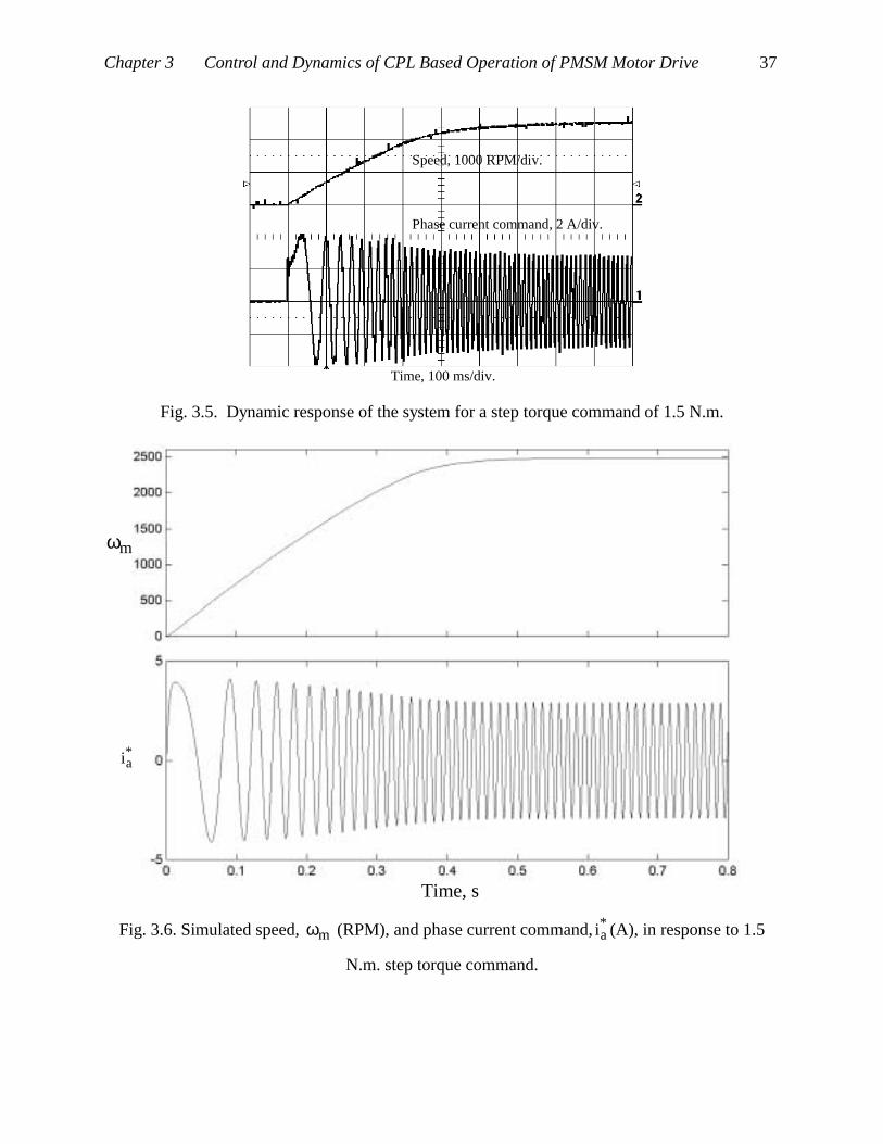
Chapter 3 Control and Dynamics of CPL Based Operation of PMSM Motor Drive 37
Time, 100 ms/div.
Speed, 1000 RPM/div.
Phase current command, 2 A/div.
Fig. 3.5. Dynamic response of the system for a step torque command of 1.5 N.m.
Time, s
mω
*ai
Fig. 3.6. Simulated speed, mω (RPM), and phase current command, *ai (A), in response to 1.5
N.m. step torque command.
Chapter 3 Control and Dynamics of CPL Based Operation of PMSM Motor Drive 38
3.8 CONCLUSIONS
A new control scheme for PMSM based on constant power loss is proposed and analyzed. It is
shown that the constant power loss operation maximizes the utilization of the machine in wide
speed range applications. A comparison of the proposed operational envelope with the
operational envelope resulting from limiting current and power to rated values is performed. It is
shown that the proposed scheme results in higher than rated torque at lower than base speed, as
well as higher than rated power in the vicinity of base speed. Overall, the proposed scheme
results in better dynamic response at lower than base speed and thermal robustness of the
machine at all operating points. It is also shown that maintaining rated power in the higher than
base speed may compromise the thermal stability of the machine. An implementation strategy for
the proposed control scheme is developed. This implementation strategy limits the torque to
correspond to the chosen power loss of the machine by employing an outer feedback loop to
control machine power losses. This has the advantage of retrofitting the present PMSM drives
with least amount of software or hardware effort. The implementation strategy does not require
any off line calculation, and is independent of the chosen control strategy for the dynamic control
of torque. The scheme lends itself to on-line implementation. The maximum permissible power
loss is the main input to the system. However, an on-line estimation of other parameters can be
input to the system in order to increase the accuracy of the power loss control system.
Experimental correlation confirms the key results of this chapter.
The contributions of this chapter are summarized below:
• A constant power loss based control strategy to obtain the maximum torque vs. speed
envelope
• Its comparison to schemes with current and power limits
• An implementation scheme for the proposed CPLC and its flexibility for incorporation in
existing drives that may have various control scheme realizations in its torque and flux
controllers
• Experimental verification of the proposed scheme
39
CHAPTER 4
The Constant Power Loss Controller for Applicationswith Cyclic Loads
4.1 INTRODUCTION
Many motion control applications require cyclic accelerations, decelerations, stops and starts.
The required movements are usually programmed into the system using a microcontroller. A
simple programmed move is the cyclic on-off operation with negligible fall and rise times. The
load duty cycle, in this case, is defined as the ratio of on time to the cycle period. In many
applications speed is constant during the on time. Usually several times average torque is
required during transitions from zero to maximum speed and vice versa. Different power losses
are generated during different phases of operation of a motor drive with cyclic loads. For
applications where the cycle period is significantly smaller than the thermal time constant of the
machine the average power loss during one cycle must be limited to the maximum permissible
value. This type of application is dealt with in this chapter. Generally speaking, the maximum
possible torque increases as the duty cycle decreases. This is due to the fact that no power loss is
generated during the off time. It is to be noted that in some applications the cycle period is large
compared to the thermal time constant of the machine. In these applications the average power
loss during one cycle in not of significant value, and instead, the instantaneous power loss during
on time must be limited to the maximum permissible value.
The objective of this chapter is to calculate the appropriate power loss command for a constant
power loss controller applied to different applications with cyclic loads. It is assumed that the
maximum permissible power loss, lmP , during continuous operation of the machine at steady
state, is known. It is also assumed that the on and off times are significantly shorter than the
thermal time constant of the machine. Five different categories of applications with cyclic loads
are considered here. In each case the power loss command must be calculated such that the
average loss over one period is equal to the maximum permissible power loss for the machine.
Chapter 4 The CPL Controller for Applications with Cyclic Loads 40
The power loss command and maximum possible torque are calculated in each case as a
function of duty cycle, maximum permissible power loss and maximum speed during one cycle.
The procedures discussed in this chapter can be applied to any application with cyclic loads.
In section 4.2 major motor drive applications are classified into five categories as far as cyclic
loads are concerned. In each category the required power loss command, average power loss,
and maximum torque during on-time, are calculated. A comparison of the maximum possible
torque vs. maximum power loss for different load categories is given in section 4.3. The
conclusions are summarized in section 4.4.
The contributions of this chapter are summarized below:
• Calculation of the appropriate power loss commands for applications with cyclic loads
• Derivation of average power loss as a function of duty cycle, maximum speed and torque for
applications with cyclic loads
• Derivation of maximum possible torque as a function of load duty cycle, maximum power
loss and maximum speed for applications with cyclic loads
• Comparison of maximum possible torque as a function of maximum possible power losses
for different applications with cyclic loads
4.2 THE POWER LOSS COMMAND IN DIFFERENTAPPLICATION CATEGORIES
A simple and practical power loss estimator for PMSM is developed here. This power loss
estimator is used in calculating the appropriate power loss command, average power loss, and
maximum possible torque, in each of five different categories of applications with cyclic loads.
Most applications fall in one of these five categories. Applications that are not covered in this
chapter can be treated using similar procedures. All torque and speed profiles are normalized
using maximum possible torque and speed in each category.
4.2.1 Derivation of a Practical Power Loss Estimator
An instantaneous power loss estimator, applicable to the surface mount PMSM, is developed
here. Note that most high performance motion control applications utilize the surface mount
PMSM. All derivations are based on the following assumptions:

Chapter 4 The CPL Controller for Applications with Cyclic Loads 41
• D-axis current is zero
• The difference between air gap and magnet mutual flux linkages is negligible
• Torque and current are proportional
• Impact of core losses on torque linearity is negligible
The above assumptions are very closely valid for the surface mount PMSM. These assumptions
are also valid for the BDCM. Therefore, the results of this chapter are readily applicable to the
BDCM. However, these assumptions are not valid for inset and interior PMSM unless these
machines are operated using the zero d-axis control strategy. The inset and interior PMSM are
only used in a small percentage of all high performance PMSM applications. Based on the
above assumptions,
ste iKT = (4.1)
where eT is the machine torque, si is the stator current magnitude, and,
aft P75.0K λ= (4.2)
The equation for the instantaneous power loss, lP , for a PMSM, can be derived using (3.5), (4.1)
and (4.2) by applying the assumptions discussed above. lP is given below,
2r2
2e1l KTKP ω+= (4.3)
where,
2t
s1
K
R5.1K = ,
c
2af
2 R
5.1K
λ= (4.4)
Note that the air gap flux linkages and magnet flux linkages are almost equal for the surface
mount PMSM. This fact is used in calculating 2K as given in (4.4).
4.2.2 *lP and emT in Different Application Categories
In this section motion control applications are broadly classified in five categories as far as
cyclic loads are concerned. In each category the required power loss command, *lP , is
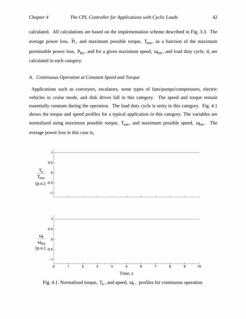
Chapter 4 The CPL Controller for Applications with Cyclic Loads 42
calculated. All calculations are based on the implementation scheme described in Fig. 3.3. The
average power loss, lP , and maximum possible torque, emT , as a function of the maximum
permissible power loss, lmP , and for a given maximum speed, rmω , and load duty cycle, d, are
calculated in each category.
A. Continuous Operation at Constant Speed and Torque
Applications such as conveyers, escalators, some types of fans/pumps/compressors, electric
vehicles in cruise mode, and disk drives fall in this category. The speed and torque remain
essentially constant during the operation. The load duty cycle is unity in this category. Fig. 4.1
shows the torque and speed profiles for a typical application in this category. The variables are
normalized using maximum possible torque, emT , and maximum possible speed, rmω . The
average power loss in this case is,
Time, s
em
eT
T
rm
rωω
(p.u.)
(p.u.)
Fig. 4.1. Normalized torque, eT , and speed, rω , profiles for continuous operation.
Chapter 4 The CPL Controller for Applications with Cyclic Loads 43
ll PP = (4.5)
where lP is the instantaneous power loss of the machine as described in (4.3). On the other
hand, the maximum average power loss is defined below,
lml PP = (4.6)
It can be seen from (4.5) and (4.6) that the maximum instantaneous power loss in steady state is
constant in this category, and is given below,
lml PP = (4.7)
Therefore, the maximum possible power loss command in this category is,
lm*l PP = (4.8)
It can be concluded from (4.3) and (4.7) that,
2rm2
2em1lm KTKP ω+= (4.9)
Therefore, the maximum possible torque, emT , for maximum power loss of lmP is,
5.0
1
2rm2lm
em )KKP
(Tω−= (4.10)
B. On-off Operation with Negligible Rise and Fall Times
This category applies to applications that run periodically in on-off mode but have negligible
rise and fall times compared to the cycle period. Some air conditioning and
fan/pump/compressor applications fall in this category. Fig. 4.2 shows an example of a torque
and speed profile in this category. In this category the operating point of the machine rises to the
desired point rapidly. Then the operating point stays constant for onT seconds. Subsequently,
the operating point drops to zero rapidly. The machine remains at this operating point for offT
seconds. The net power loss during rise and fall of the operating point is negligible as compared

Chapter 4 The CPL Controller for Applications with Cyclic Loads 44
to the losses during on time. These applications may require higher than rated torque during the
short rise and fall periods.
em
eTT
rm
rωω
Time, s
(p.u.)
(p.u.)
onT offT
Fig. 4.2. Normalized torque and speed profiles for on-off operation with small transition times.
The average power loss in this case is,
dPTT
TPP l
offon
onll =
+= (4.11)
where lP is the power loss during on time. On the other hand, the maximum average power loss
is defined below,
lml PP = (4.12)
It can be concluded from (4.11) and (4.12) that, while operating at maximum average power loss,

Chapter 4 The CPL Controller for Applications with Cyclic Loads 45
lml PdP = (4.13)
Therefore, the maximum power loss command during on time is defined below,
dP
P lm*l = (4.14)
The maximum torque during on time, emT , can be calculated by substituting (4.3) into (4.13) as
given below:
lm2rm2
2em1 Pd)KTK( =ω+ (4.15)
5.0
1
2rm2lm
em )K
KdP(T
ω−= (4.16)
C. Speed Reversal Operation with Negligible Transition Times
In some motion control systems, such as pick and place applications and automatic welding
machines, the end-effector is moving in between jobs most of the time while the actual task takes
a relatively short time for completion. Therefore, the power loss during the actual task time is
negligible compared to the average power loss during one full cycle. The speed of the end-
effector is almost constant while moving in between jobs. Fig. 4.3. shows a typical torque and
speed profile of an application in this category. As far as the net power loss is concerned this
profile and the profile described in section A are the same. Therefore, the maximum power loss
command can be calculated, using (4.8), as given below,
lm*l PP = (4.17)
Similarly, the average power loss, under extreme conditions, is described as,
lml PP = (4.18)
The maximum possible torque, emT , for maximum power loss of lmP and speed of rmω , is,
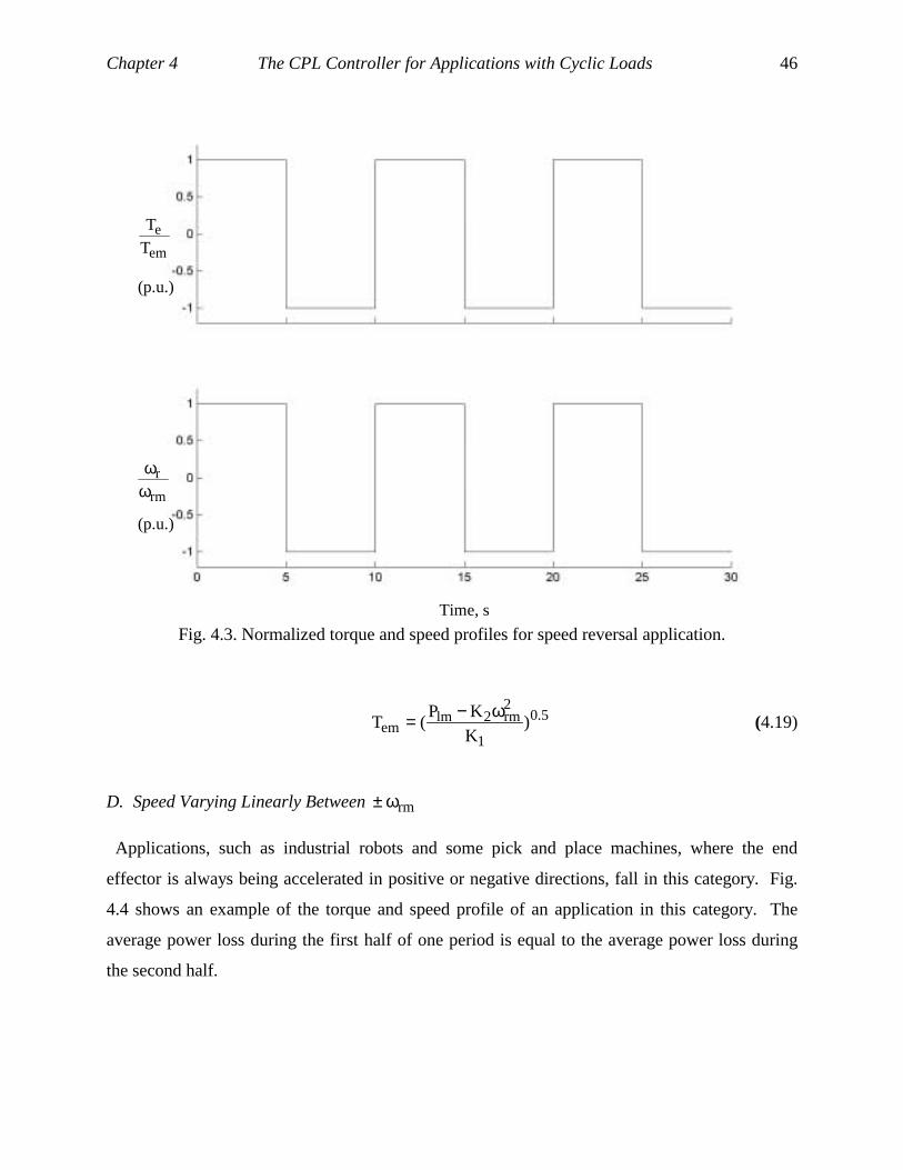
Chapter 4 The CPL Controller for Applications with Cyclic Loads 46
Time, s
em
eTT
rm
rωω
(p.u.)
(p.u.)
Fig. 4.3. Normalized torque and speed profiles for speed reversal application.
5.0
1
2rm2lm
em )KKP
(Tω−= (4.19)
D. Speed Varying Linearly Between rmω±
Applications, such as industrial robots and some pick and place machines, where the end
effector is always being accelerated in positive or negative directions, fall in this category. Fig.
4.4 shows an example of the torque and speed profile of an application in this category. The
average power loss during the first half of one period is equal to the average power loss during
the second half.
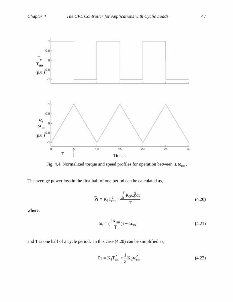
Chapter 4 The CPL Controller for Applications with Cyclic Loads 47
(p.u.)
(p.u.)
em
eTT
rm
rωω
Time, sT
Fig. 4.4. Normalized torque and speed profiles for operation between rmω± .
The average power loss in the first half of one period can be calculated as,
T
dtKTKP
T0
2r22
em1l∫ ω
+= (4.20)
where,
rmrm
r t)T
2( ω−ω=ω (4.21)
and T is one half of a cycle period. In this case (4.20) can be simplified as,
2rm2
2em1l K
31
TKP ω+= (4.22)

Chapter 4 The CPL Controller for Applications with Cyclic Loads 48
In this category the instantaneous power loss estimation changes with speed throughout every
period. If the power loss controller’s PI block operates on the difference of the power loss
command and the instantaneous power loss estimation, then the resulting torque limit varies
linearly within one cycle of operation. However, as seen in Fig. 4.4, the torque needs to be
constant during each half period of one full cycle. The solution to this problem is to use a low
pass filter with a large time constant on the output of the power loss estimator (see Fig. 3.3).
Such a filter should effectively output the average power loss of the machine in steady state.
Under these conditions the maximum power loss command, that can limit the average power loss
to lmP , can be described as,
lm*l PP = (4.23)
Since the maximum average power loss must not exceed lmP , it can be concluded from (4.22)
that,
lm2rm2
2em1 PK
31
TK =ω+ (4.24)
The maximum possible torque can then be calculated from (4.24) as,
5.0
1
2rm2lm
em )K
KP3(T
ω−= (4.25)
E. On-off Operation with Significant Rise and Fall Times
Industrial lifts, elevators, and some pumps, fans and servo drives are examples that fall in this
category. For these applications the speed rises to a target level while several times rated torque
is being applied. Speed and torque remain constant for a period of time. Then the speed is
reduced to zero which again requires several times rated torque. The operating point stays in this
state for a period of time. The power losses during rise and fall times, in this category, constitute
a significant portion of the average power loss.

Chapter 4 The CPL Controller for Applications with Cyclic Loads 49
Time, s
rm
rωω
em
eTT
em
ep
T
T
em
ep
T
T−
1pT∆ mT∆
2pT∆zT∆
(p.u.)
(p.u.)
Fig. 4.5. Normalized torque and speed profiles for operation with significant transition times.
Fig. 4.5 shows a typical torque and speed profile in this category. A peak torque of epT N.m. is
applied for 1pT∆ seconds at the beginning of each cycle to raise the speed to the desired value of
rmω . Then speed is maintained constant for a period of mT∆ seconds during which time a
constant torque of emT N.m. is applied to the load. Finally, speed is brought back to zero by
applying epT− N.m. for a period of 2pT∆ seconds. The speed remains at zero for a period of
zT∆ seconds.
The magnitude of peak torque is set by the peak torque limiter block of Fig. 3.3. The power
loss command, *lP , is set at maximum value during the peak torque periods in order to saturate
the power loss PI controller. Saturation of this PI controller allows the torque to be limited by
Chapter 4 The CPL Controller for Applications with Cyclic Loads 50
the peak torque limiter block of Fig. 3.3. The power loss command during the mT∆ seconds
where nominal torque is being applied must be calculated as follows. The average power loss in
this case is calculated by adding the energy losses in each segment, and dividing the result by the
time period of one cycle. The net energy loss, lW , in one cycle can be described as,
2p2rm2
2ep1m
*l1p
2rm2
2ep1l T)K
31
TK(TPT)K31
TK(W ∆ω++∆+∆ω+= (4.26)
The average power loss in one cycle is,
T
W
TTTT
WP l
z2pm1p
ll =
∆+∆+∆+∆= (4.27)
where T is the cycle period. The average power loss should not exceed lmP . Therefore,
lml PP = (4.28)
It can be concluded from (4.26), (4.27) and (4.28) that
2p2rm2
2ep1m
*l1p
2rm2
2ep1lm T)K
31
TK(TPT)K31
TK(TP ∆ω++∆+∆ω+= (4.29)
Therefore, the required *lP during the mT∆ period can be calculated from (4.29) as,
m
2p2rm2
2ep11p
2rm2
2ep1lm*
l T
T)K31
TK(T)K31
TK(TPP
∆
∆ω+−∆ω+−= (4.30)
In brief, the power loss command is set at maximum during the transitional periods, and is set at
the value calculated in (4.30) for the steady state period.
The power loss during the steady state period is,
)KTK(P 2rm2
2em1l ω+= (4.31)
Chapter 4 The CPL Controller for Applications with Cyclic Loads 51
where lP is calculated from (4.30), and is equal to *lP in steady state. Therefore, the maximum
possible torque during the mT∆ period in Fig. 4.5 is,
5.0
1
2rm2
*l
em )KKP
(Tω−= (4.32)
An alternative to the CPL implementation scheme described in Chapter 3 is to program the
torque limiter to limit the torque to maximum desirable values during transition periods, and to
limit the torque the value given in (4.32) during nominal operation. In this case the power loss
control loop is not required. Similarly, the torque limiter can be utilized in limiting the average
power loss in other application categories without resorting to the power loss feedback control
loop. However, having a power loss control loop is preferred in the first four categories because
of the simplicity of its implementation and the simplicity involved in calculating the power loss
command in those categories.
4.3 COMPARISON OF MAXIMUM TORQUE IN DIFFERENT CATEGORIES
It can be concluded from the previous discussion that the maximum possible torque is a
function of maximum possible power loss, load duty cycle and the nature of the cyclic load. In
this section the maximum possible torque as a function of lmP and load duty cycle is calculated
and compared for the load categories A to E as discussed in sections 4.2.a to 4.2.e. The
parameters of the motor drive given in Appendix I are used for this purpose. It is assumed that
the zero d-axis current control strategy is adopted so that the assumptions given in section 4.2.1
are valid. The maximum speed is set at rated speed in all cases. The load categories A to D are
dealt with in section 4.3.1. The load category E is dealt with separately in section 4.3.2. due the
large number of variables that can affect the maximum possible torque in that category.
4.3.1 Load Categories A to D
Figure 4.6. shows the maximum torque vs. maximum power loss profiles for load categories A
to D. The maximum torque vs. maximum power losses equations derived in sections 4.2a to
4.2.d have been used in preparing the profiles for load categories A to D, respectively.

Chapter 4 The CPL Controller for Applications with Cyclic Loads 52
Fig. 4.6. Maximum torque vs. maximum power loss for load categories A, B, C and D for duty
cycles equal to 1, 0.75, 0.5, 0.33.
Load categories A and C result in identical maximum torque vs. maximum power loss profiles.
The maximum torque is the lowest in these categories due to the lack of any off time. Load
category B with load duty cycle of 1 also results in the same profile as that of load categories A
and C. However, as duty cycle is lowered the maximum possible torque for a given maximum
power loss consistently increases. The torque vs. power loss profile for load category D is the
same as that of load category B with a duty cycle of 0.333. This can be seen by comparing
(4.25) and (4.16). In each load category there is a minimum power loss below which no torque
can be produced. This is due to the fact that the maximum possible power loss should exceed the
net core losses generated within each period so that a nonzero magnitude of copper losses can be
tolerated. Note that generation of torque is not possible if copper losses are not allowed.
lmP
emT
A , C, or B with d=1
B with d=0.75
B with d=0.5
B with d=0.33, or D
lmP
emT
A , C, or B with d=1
B with d=0.75
B with d=0.5
B with d=0.33, or D
lmP
emT
A , C, or B with d=1
B with d=0.75
B with d=0.5
B with d=0.33, or D
lmP
emT
A , C, or B with d=1
B with d=0.75
B with d=0.5
B with d=0.33, or D
lmP
emT
A , C, or B with d=1
B with d=0.75
B with d=0.5
B with d=0.33, or D
lmP
emT
A , C, or B with d=1
B with d=0.75
B with d=0.5
B with d=0.33, or D
p.u.,Plm
p.u.,Tem
A , C, or B with d=1
B with d=0.75
B with d=0.5
B with d=0.33, or D
p.u.,Plm
p.u.,Tem
A , C, or B with d=1
B with d=0.75
B with d=0.5
B with d=0.33, or D

Chapter 4 The CPL Controller for Applications with Cyclic Loads 53
4.3.2. Load Category E
The maximum possible torque for applications with significant rise and fall times is a function
of maximum possible power loss, load duty cycle, peak torque requirements and duration of rise
and fall times. In this section a sample calculation of maximum possible torque for such an
application using the prototype motor drive discussed in Appendix I is given. The peak torque is
assumed to be twice the rated torque, and the duration of rise and fall times are 2 seconds each.
The entire period is 20 seconds, and the machine is at idle for 6 seconds. This leaves 10 seconds
during which torque is applied to the application while speed is constant at the target value. The
objective is to find the maximum possible torque during this period. Equation (4.30) yields a
maximum possible power loss of 93.1 W during this period. The maximum possible torque is
0.84 p.u. in this case using (4.32). If the on time is reduced to 8 seconds instead of 10 seconds
then the maximum possible torque rises to 0.98 p.u. An on time of 6 seconds results in a
maximum possible torque of 1.19 p.u. Note that the power losses during the transition times do
not change as duty cycle changes since the maximum torque during transition time is fixed.
It is clear from the above discussion that the calculation of maximum possible torque in the case
of applications with load profiles such as the one shown in Fig. 4.5 is subjective and needs to be
dealt with on case by case basis as shown above.
4.4 CONCLUSIONS
A large number of motion control applications involve cyclic and programmable movements.
The procedure for adapting the constant power loss controller, as described in Chapter 3, to
applications that involve cyclic movements is discussed in this chapter. The maximum
permissible power loss, lmP , for a machine has been previously defined to be valid only for
constant speed and torque operation. In this chapter the power loss command is calculated as a
function of duty cycle, lmP and maximum speed in five different categories of applications with
cyclic loads such that the average power loss does not exceed lmP . These categories are: A.
constant torque and speed, B. on-off operation at constant speed and torque at a specific duty
cycle, C. speed reversal with constant torque and speed magnitudes at a specific duty cycle, D.
cyclic ramping operation between two speeds with constant magnitude of torque, E. general

Chapter 4 The CPL Controller for Applications with Cyclic Loads 54
torque vs. speed profiles. It is shown that in load categories A and C the power loss command is
equal to lmP . In load category B the power loss command is equal to lmP divided by the duty
cycle. In load categories A, B and C the power loss estimator filter can be a simple filter to
remove noise, and should yield the instantaneous net power loss of the machine. The power loss
command in load category D is equal to lmP . It is shown that, in this case, the power loss
estimator filter must yield the average of the net power loss in one cycle instead of the
instantaneous power loss. In load category E each subsection in one cycle has its own maximum
possible torque. Therefore, the power loss command in each subsection is different.
Consequently, the power loss command must be programmed as a function of the desired torque
vs. speed profile in this category. Instantaneous power loss estimation is required in this
category. In each of the five categories the average power loss and maximum possible torque as
a function of lmP , speed and duty cycle are calculated. All load categories are compared based
on maximum possible torque as a function of maximum possible power loss and load duty cycle.
A similar approach, as outlined in this chapter, can be applied to applications that involve more
complex torque and speed profiles.
The contributions of this chapter are summarized below:
• Calculation of the appropriate power loss command for applications with cyclic loads
• Derivation of average power loss as a function of duty cycle, maximum speed and torque for
applications with cyclic loads
• Derivation of maximum possible torque as a function of duty cycle, maximum power loss
and maximum speed for applications with cyclic loads
• Comparison of maximum possible torque as a function of maximum possible power losses
for different applications with cyclic loads

55
CHAPTER 5
Performance Evaluation and Comparison of
Control Strategies 5.1 INTRODUCTION
Vector control of PMSM allows for the implementation of several choices of control strategies
while control over torque is retained. The main control strategies for the lower than base speed
operating range are:
(a) Maximum efficiency (ME)
(b) Maximum torque per unit current (MTPC)
( c) Zero d-axis current (ZDAC)
(d) Unity power factor (UPF)
(e) Constant mutual flux linkages (CMFL)
The main control strategies for the higher than base speed operating range are:
(a) Constant back emf (CBE)
(b) Six-step voltage (SSV)
Each of these control strategies are described and analyzed in this chapter. The procedure for
deriving the q and d-axis current commands as a function of torque and speed is described in
each case. Also, the procedure for deriving the maximum possible torque vs. speed profile for a
given maximum possible power loss is described for each control strategy. Subsequently, a
comprehensive comparison of these control strategies is made. The main part of the comparison
is based on operation along the maximum possible torque vs. speed envelope. The maximum
possible torque vs. speed envelope depends on the maximum possible power loss, and is also a
function of the chosen control strategy as well as motor drive parameters. Therefore, each
Chapter 5 Performance Evaluation and Comparison of Control Strategies
56
control strategy results in a unique operational envelope for a given machine. Consequently, the
performance of the system under each control strategy is also unique. Maximum torque,
current, power, torque per unit current, back emf and power factor vs. speed are the key
performance indices that are used here to compare different control strategies. Current, air gap
flux linkages, and d-axis current vs. torque are also compared in each case in order to provide
insight into the performance of the system inside the operational boundary. It is assumed here
that the maximum possible power loss is constant for the full range of operating speed. This
assumption is made in order to simplify the demonstrations and analytical derivations, and to be
able to present the fundamental concepts with better clarity. Similar procedures can be used to
analyze and compare different control strategies for an arbitrary maximum possible power loss
vs. speed profile. The procedures provided in this study can be used to choose the optimal
control strategy based on the requirements of a particular application and also based on the
capabilities of the chosen motor drive. The fundamental concepts and procedures are emphasized
in this chapter, while non-critical analytical derivations are delegated to Chapter 8.
The contributions of this chapter are summarized below:
• Performance analysis of different control strategies for PMSM along the constant power loss
operational envelope
• Comparison of control strategies along the constant power loss operating envelope
• Comparison of control strategies inside the operating envelope
• Derivation of absolute maximum torque for the unity power factor and constant mutual flux
linkages control strategies
• Derivation of maximum speed, current and torque in the flux weakening range as a function
of maximum power loss and machine parameters.
• Experimental verification of key results
Section 5.2 describes a complete set of performance criteria. Section 5.3 reviews the analytical
details of the five control strategies applicable to a high performance PMSM control system in
the lower than base speed operating range. The two possible control strategies for the higher
than base speed operating range are studied in section 5.4. The performances of control
Chapter 5 Performance Evaluation and Comparison of Control Strategies
57
strategies along the constant power loss operational envelope are compared in section 5.5. The
performances of control strategies inside the operational envelope are compared in section 5.6.
The procedure used to study torque ripple under the SSV control strategy is described in section
5.7. Simulation and experimental verification of the key results of this chapter are given in
section 5.8. The conclusions are discussed in section 5.9.
5.2 PERFORMANCE CRITERIA
The performance criteria discussed below are the most relevant as far as this study is concerned.
These criteria are used in later sections to evaluate and compare the performances of different
control strategies for the full range of operational speed.
(a) Torque, current and voltage: These three variables are among the most fundamental
performance criteria in motor drives. The basic function of a motor drive is to deliver the torque
required by an application. It is desirable to produce a higher magnitude of torque within the
given constraints of a motor drive to make the same drive applicable to a wider range of
applications. These constraints include voltage and current limitations as well as maximum
permissible power loss. Lower current and voltage requirements translate into cost savings as far
as the drive is concerned.
(b) Back emf: This is the voltage induced in the windings by the rotating magnetic field in the air
gap. Basically, the phase voltage has to work against the back emf in order to enforce a desired
current. For most analytical purposes, specially at higher than base speeds, the fundamental
component of the back emf and that of the phase voltage can be assumed to be approximately the
same in steady state. The small difference is due to the voltage drop across the phase resistance.
(c) Maximum torque vs. speed profile: This profile is frequently used to match a motor drive to
an application. A larger and wider torque vs. speed profile results in the motor drive being
suitable for a wider range of applications.
(d) Power: Amount of work delivered divided by time. This performance index is also referred
to as real power.
Chapter 5 Performance Evaluation and Comparison of Control Strategies
58
(e) Volt Ampere: The product of phase voltage and phase current multiplied by the number of
phases. Also referred to as apparent power.
(f) Power factor: Power divided by Volt Ampere. A measure of the level of utilization of the
available apparent power.
(g) Power loss: This index can include copper and core losses, drive losses, windage, friction and
stray losses of a machine. The maximum permissible power loss influences the operational
boundary of a motor drive.
(h) Efficiency: Shaft power divided by input power. This is a very critical index for many
applications.
(i) Torque per unit current: A higher value of this index indicates that more torque is being
produced for a given magnitude of current.
(j) Torque per unit power loss: A higher value of this index indicates that more torque is being
produced for a given net power losses.
(k) Air gap flux linkages: The net flux linkages crossing the air gap. The product of this index
and electrical speed is back emf. Core losses depend on flux linkages, speed and machine
parameters. Flux linkages are also important from the point of view of magnetic saturation.
(l) d-axis current: d-axis current results in flux linkages along the same path as the magnet's flux
linkages. This current must be limited to the maximum value beyond which the magnets get
partially demagnetized. Therefore, dI serves as an index that needs to be monitored and limited.
(m) Base speed: The speed at which the back emf reaches the maximum possible value along the
maximum torque vs. speed envelop is defined here as base speed. The base speed is a function
of motor parameters, maximum voltage available to the phase, and the control strategies used in
the lower and higher than base speed operating ranges.
(n) Maximum speed: The maximum speed attainable by a motor drive. By definition zero torque
is produced at this maximum speed.
(o) Complexity of implementation: This indicator is used to compare different control strategies
from the point of view of implementation requirements.

Chapter 5 Performance Evaluation and Comparison of Control Strategies
59
(p) Current and torque ripples: Current ripple is caused mainly by the drive’s current control
mechanism, or lack of control over current. Machine and drive imperfection also result in
current ripple, but analysis of this type of ripple is beyond the scope of this dissertation. The
drive’s current control mechanism usually results in a low percentage of current ripple with
frequencies in the range of 10 to 30 kHz for common applications. Lack of control over current
usually results in higher magnitudes of ripple with frequencies that are proportional to speed.
Current ripples translate into torque ripples directly.
(q) Cost: This is the most fundamental criteria in motor drives as well as in any other
commercial product. A motor drive must be designed such that the overall cost is minimum
while it meets or exceeds the requirements of an application. The overall cost includes cost of
design, material, manufacturing requirements, warranties and service.
5.3 CONTROL STRATEGIES: LOWER THAN BASE SPEED OPERATING RANGE
The most important objective of high performance control strategies is to maintain linear
control over torque. Therefore, qi and di must be coordinated to satisfy the equation given
below for a desired torque, eT ,
)ii)LL(i(P75.0T qdqdqafe −+λ= (5.1)
However, it can be seen from (5.1) that a wide range of qi and di values yield the same torque.
Each of the five control strategies discussed in sections 5.3.1 to 5.3.5 utilize the available degree
of freedom, seen in (5.1), to meet a particular objective. Equation (5.2) shows the general
description of the intended relationship between currents, qi and di , and torque and speed, eT
and rω , respectively, for a given control strategy,
Chapter 5 Performance Evaluation and Comparison of Control Strategies
60
ωΓ
ωΛ=
),T(
),T(
i
i
re
re
d
q (5.2)
where Λ and Γ represent the relationship described by (5.1) in combination with the objective
of the specific control strategy. At any given speed the maximum possible torque is limited by
the maximum possible power loss, lmP . Therefore, qi and di must satisfy the following
equation while the system is operating at maximum torque,
])iL()iL[(R
5.1)ii(R5.1P 2
ddaf2
qq2r
c
2ds
2qsslm +λ+ω++= (5.3)
where, qsi and dsi are defined as a function of qi and di in (3.1). In this chapter the maximum
possible torque at any given speed is studied for different control strategies. Chapter 8 addresses
the analytical details of the derivations involved in calculating the maximum torque vs. speed
profiles. Generally, the maximum possible torque is a function of speed, maximum possible loss
and the chosen control strategy, as described below:
)P,(T lmrem ωΥ= (5.4)
where emT is the maximum possible torque, and the function Υ depends on the chosen control
strategy and machine parameters.
The maximum torque under the maximum efficiency, maximum torque per unit current and
zero d-axis current control strategies is only limited by the maximum possible power loss for the
motor. However, each of the unity power factor and constant mutual flux linkages control
strategies impose an absolute maximum possible torque, as described in sections 5.3.4 and 5.3.5,
respectively. Therefore, for the latter two control strategies, the maximum possible torque is the
smaller of the respective absolute maximum torque and the maximum torque resulting from the
power loss limitation.

Chapter 5 Performance Evaluation and Comparison of Control Strategies
61
5.3.1 Maximum Efficiency Control Strategy (ME)
qi and di are coordinated to minimize net power loss, lP , at any operating torque and speed.
The net power loss can be described as given below,
])iL()iL[(R
5.1)ii(R5.1P 2
ddaf2
qq2r
c
2ds
2qssl +λ+ω++= (5.5)
where,
ωλ+
ω−
ω
=
0 R
i
i
1 R
LR
L 1
i
ic
raf
d
q
c
rq
c
rd
ds
qs (5.6)
The optimal set of currents, qi and di , that result in minimization of power loss at a given
speed and torque can be found using (5,1), (5.5) and (5.6). This operation can be performed
using numerical methods. Alternatively, an analytical solution, that yields (5.2) for this control
strategy, is given in Chapter 8.
Equation (5.5) is a simplified representation of the sum of copper and core losses. In practice a
more accurate representation of core losses, based on elaborate equations or tables, can be used
to increase the accuracy of the total loss estimation. Other types of losses, such as drive losses,
friction, windage and stray losses, can also be included. More accurate equations for core losses
can be found in [13, 14].
Minimizing lP at zero speed results in minimizing copper losses since core losses are zero at
zero speed. On the other hand, minimizing copper losses is equivalent to minimizing current.
Therefore, the maximum efficiency control strategy results in minimum current for a given
torque at zero speed, which means that the ME and MTPC control strategies result in identical
performance at zero speed.
Chapter 5 Performance Evaluation and Comparison of Control Strategies
62
5.3.2 Zero d-axis Current Control Strategy (ZDAC)
The torque angle is defined as the angle between the q-axis current and the d-axis in the rotor
reference frame. This angle is maintained at 90 degrees in the case of the ZDAC control
strategy. The ZDAC control strategy is the most widely utilized control strategy by the industry.
The d-axis current is effectively maintained at zero in this control strategy. The main advantage
of this control strategy is that it simplifies the torque control mechanism by linearizing the
relationship between torque and current. This means that a linear current controller results in
linear control over torque as well. In dc motors the current and magnet fields are always
maintained at an angle of 90 degrees. Therefore, the ZDAC control strategy makes a PMSM
operate in a similar way to the dc motor. This makes the ZDAC control strategy very attractive
for industrial designers who are used to operating dc motor drives. The following relationships
hold for the ZDAC control strategy:
safe iP75.0T λ= (5.7)
where si is the phase current magnitude, and
sq ii = (5.8)
0id = (5.9)
The current, si , for a given torque, eT , can be calculated as,
af
es P75.0
Ti
λ= (5.10)
The air gap flux linkages can be described as,
5.02s
2d
2afm )iL( +λ=λ (5.11)
The ZDAC control strategy is the only control strategy that enforces zero d-axis current. This
is one of the disadvantages of this control strategy as compared to the other four control
strategies. A non-zero d-axis current has the advantage of reducing the flux linkages in the d-
Chapter 5 Performance Evaluation and Comparison of Control Strategies
63
axis by countering the magnet flux linkages. This serves to generate additional torque for inset
and interior PMSM, and also reduces the air gap flux linkages. Lower flux linkages result in
lower voltage requirements as well. Therefore, application of the ZDAC control strategy results
in higher air gap flux linkages and higher back emf as compared to other control strategies. The
maximum possible torque under this control strategy is only limited by the maximum possible
power loss.
5.3.3 Maximum Torque per Unit Current Control Strategy (MTPC)
The MTPC control strategy is the most widely studied control strategy by the research
community. Application of this control strategy results in the production of maximum possible
torque at any given current. This control strategy minimizes current for a given torque.
Consequently, copper losses are minimized in the process. The additional constraint imposed on
qi and di for motors with magnetic saliency is:
)LL
i(iiqd
afdd
2q −
λ+= , qd LL ≠ (5.12)
For the types of PMSM that do not exhibit magnetic saliency the MTPC and ZDAC control
strategies are the same. The MTPC control strategy results in maximum utilization of the drive
as far as current if concerned. This is due to the fact that more torque is delivered for unit
current as compared to other techniques. The MTPC and ME control strategies result in
identical current commands at zero speed. The maximum possible torque under this control
strategy is only limited by the maximum possible power loss.
5.3.4 Unity Power Factor Control Strategy (UPF)
Power factor can be defined as given below if the voltage drop across the phase resistance is
ignored,
)EIcos()cos(pf ∠−∠=θ= (5.13)
where I and E are the current and back emf phasors, respectively, and “∠ ” denotes the angle
of the respective phasor. The angle θ can be described as,

Chapter 5 Performance Evaluation and Comparison of Control Strategies
64
)i
i(tan)
iLiL
(tand
q1
ddaf1 −− −−
+λ=θ (5.14)
Unity power factor can be achieved by maintaining the following relationship between qi and
di ,
0iiLiL daf2qq
2dd =λ++ (5.15)
This control strategy imposes an absolute maximum possible torque on the system. This
maximum permissible torque is found by inserting qi as a function of di from (5.15) into the
torque equation (5.1), and differentiating torque with respect to di . By differentiating this
equation and equating it to zero the d-axis current, dmI , that yields the maximum possible
torque, emT , is derived. The following equation yields dmI ,
0II dm2dm =γ+β+α (5.16)
where,
dqd L)LL(4 −=α
dafafqd L2)LL(3 λ+λ−=β
2afλ=γ
Inserting dmI into (5.15) yields the q-axis current, qmI , at absolute maximum torque. Inserting
qmI and dmI in (5.1) yields the absolute maximum torque possible under the UPF control
strategy.
5.3.5 Constant Mutual Flux Linkages Control Strategy (CMFL)
By maintaining a constant air gap flux linkages the machine is protected against magnetic
saturation. Also, the maximum speed after which flux weakening becomes necessary is
extended. The most common choice is to maintain the air gap flux linkages at the magnet’s flux
linkages value. In this case equation (5.17) must hold.

Chapter 5 Performance Evaluation and Comparison of Control Strategies
65
2qq
2ddaf
2af )iL()iL( ++λ=λ (5.17)
This control strategy imposes an absolute maximum torque on the system. This maximum
permissible torque is found by inserting qi as a function of di from (5.17) into the torque
equation (5.1), and differentiating torque with respect to di . By differentiating this equation and
equating it to zero the d-axis current, dmI , that yields the maximum possible torque, emT , is
derived. The following equation yields dmI in this case,
0III dm2dm
3dm =ϑ+γ+β+α (5.18)
where,
2qd
2d )LL(L4 −=α
)LL2)(LL(L6 qdqddaf −−λ=β
)L4L5(L2 qd2afd −λ=γ
d3af L2λ=ϑ
The smallest real and negative solution of (5.18) is the right choice. qmI can then be calculated
by inserting dmI into (5.17). Inserting dmI and qmI into (5.1) yields the absolute maximum
possible torque under the CMFL control strategy. This maximum torque is usually very high for
PMSM, and requires excessive current.
5.4 CONTROL STRATEGIES: HIGHER THAN BASE SPEED OPERATING RANGE
The fundamental component of phase voltage is constant in the higher than base speed, or flux
weakening, operating range. Voltage restriction, as well as the requirement for torque linearity,
limit the number of possible control strategies in the flux weakening range. The main
possibilities in this range are the six-step voltage (SSV) and constant back emf (CBE) control
strategies. The CBE control strategy limits the back emf to a desired value such that a constant
voltage margin is preserved throughout the flux weakening range. This margin allows the
system to retain instantaneous control over current and torque in the flux weakening range. In

Chapter 5 Performance Evaluation and Comparison of Control Strategies
66
this range back emf and instantaneous torque are controlled by coordinating the current phasor’s
magnitude and angle with respect to the rotor. This type of control is only suitable for a limited
spectrum of high performance applications that require high quality control over torque at higher
than base speed. In the SSV control strategy maximum possible voltage is always applied to the
phases, and only the average torque can be controlled. The average torque is controlled by
varying the angle of voltage phasor with respect to the rotor’s magnetic field.
In this section the CBE and SSV control strategies are analyzed. The operational envelope,
current requirements and maximum speed are studied in each case based on the concept of
constant power loss. Current and torque ripples are also studied in each case. The maximum
torque vs. speed envelope for both control strategies is found by limiting the net power loss of
the machine to a desired level. The motor always operates within a safe thermal boundary by
limiting the net power loss to a desired value. The most dominant types of power losses, which
are core and copper losses, are included in this analysis. Analytical derivations of the maximum
speed and maximum current requirement in the flux weakening range are derived for each
control strategy. The fundamental current ripple for the CBE control strategy is the result the
enforcement of instantaneous control over current. The fundamental current ripple for the SSV
control strategy results from the lack of instantaneous control over current. A procedure for
deriving the instantaneous phase current and torque waveforms in steady state under the SSV
control strategy is given for PMSM. This procedure is an application of the analysis presented in
[34].
Section 5.4.1 provides the basics of the CBE control strategy. The details of the SSV control
strategy are presented in section 5.4.2.
5.4.1 Constant Back emf Control Strategy
The CBE control strategy is discussed here. The operational envelope and current requirements
of the system are studied.

Chapter 5 Performance Evaluation and Comparison of Control Strategies
67
A. The Basics
In this mode the d and q axis currents, qi and di , respectively, are coordinated to achieve a
desired constant back emf as well as torque linearity. qi and di need to satisfy equations (5.19)
and (5.20) in steady state at a given speed, rω , and for a desired back emf, mE , and a desired
torque, eT .
2qq
2ddaf
2
r
m )iL()iL()E
( ++λ=ω
(5.19)
)ii)LL(i(P75.0T dqqdqafe −+λ= (5.20)
Equation (5.19) ensures that the back emf remains constant at a desired value mE . Equation
(5.20) ensures torque linearity. Note that in the flux weakening range each of the two currents is
a function of both speed and torque as described below,
ωΓ
ωΛ=
),T(
),T(
i
i
re
re
d
q (5.21)
where Λ and Γ represent the relationships as described by (5.19) and (5.20). The
implementation of these equations can be performed in software or using programmable read-
only memory chips utilized as two dimensional look-up tables in hardware [44].
B. Maximum Current in the Flux Weakening Range
The maximum current in a machine in steady state is determined by the designed maximum
permissible power loss. The electrical power losses in a machine are copper and core losses.
Equation (5.22) provides a simplified estimation of the net power loss for a PMSM.
2m
2r
c
2ssl R
5.1IR5.1P λω+= (5.22)

Chapter 5 Performance Evaluation and Comparison of Control Strategies
68
where mλ is the air gap flux linkages as described below,
5.02qq
2ddafm ])IL()IL[( ++λ=λ (5.23)
The second term on the right hand side of (5.22) represents the core losses of the motor.
The product of speed and air gap flux linkages is equal to the desired constant back emf in the
flux weakening range. On the other hand the maximum permissible torque at a given speed
occurs when the net power loss is equal to the maximum permissible power loss, lmP . lmP is
assumed to be a constant for the full range of operating speed. Therefore, it can be concluded
from (5.22) that,
c
2m2
smslm RE5.1IR5.1P += (5.24)
where, smI is the value of current along the operational boundary. It is noted that the core losses
are constant in the flux weakening range as the induced emf is kept a constant. This is seen from
the part of (5.24). Therefore, for constant net power loss, the phase current magnitude is also a
constant and this is inferred from (5.24) as well. Equation (5.24) defines the current requirement
in the flux weakening range as a function of maximum permissible power loss and desired back
emf for the CBE control strategy.
C. Operational Boundary
The maximum possible torque at a given speed in the flux weakening range is the torque that
results in maximum possible power loss. The current phasor at which maximum torque is
produced while both back emf and net power loss are at maximum level must satisfy equations
(5.25) and (5.26) as described below,
2qmq
2dmdaf
2
r
m )IL()IL()E
( ++λ=ω
(5.25)

Chapter 5 Performance Evaluation and Comparison of Control Strategies
69
cs
2m
s
lm2qm
2dm
2sm RR
ER5.1
PIII −=+= (5.26)
where the current phasor is the resultant of q and d axis currents, qmI and dmI , respectively, at
maximum torque. Note that it is assumed that the rotor current and phase current are
approximately equal as discussed in section 3.7. Inserting qmI and dmI into (5.20) gives the
maximum permissible torque at speed rω . Therefore, the operational envelope can be described
as,
)P,(T lmrem ωΦ= (5.27)
where Φ represents the concurrent solution of (5.25), (5.26) at (5.20) at a given speed.
D. Maximum Speed in the Flux Weakening Range
At maximum speed torque is zero. At this operating point maximum possible current is utilized
to counter the magnet flux linkages, and qI is zero. Therefore, it can be concluded from (5.25)
that the maximum speed is given as,
5.0
sc
2m
s
lmdaf
m
smdaf
mrm
)RR
ER5.1
P(L
EIL
E
−−λ
=−λ
=ω (5.28)
where, rmω is the maximum speed, and smI is given in (5.26).
5.4.2. Six Step Voltage Control Strategy
An alternative to the CBE control strategy is the six step voltage (SSV) control strategy. In this
control strategy full bus voltage is applied to the motor. In this case the phase voltage is quasi-
sinusoidal with six steps such as the one shown later in Fig. 5.1. Average torque is controlled by

Chapter 5 Performance Evaluation and Comparison of Control Strategies
70
varying the angle of the voltage phasor with respect to the rotor field. The magnitude of the
voltage phasor is determined by the dc bus voltage.
A. Fundamental Analysis
The average torque produced in SSV mode can be calculated from the fundamental component
of the six step input voltage. This is based on the fact that only the fundamental components of
variables contribute to the average torque. The peak of the fundamental component of voltage,
mV , available to the motor phase for a 3-phase star-connected motor with a full bridge power
stage is described as,
dcm V)2
(Vπ
= (5.29)
where, dcV is the bus voltage. The fundamental components of q-axis and d-axis voltages in the
rotor reference frame, qsV and dsV , can be expressed as,
)sin(VV mqs α= (5.30)
)cos(VV mds α= (5.31)
where α is the angle of the voltage phasor with reference to the rotor's d-axis. The voltage drop
across the stator resistance is negligible since this voltage drop is small relative to phase voltage
in the flux weakening range. Therefore, qV and dV in steady state can be described as,
)IL( V ddafrqs +λω= (5.32)
qqrds ILV ω−= (5.33)
The axes currents can be derived from (5.30)-(5.33) and inserted in (5.20) resulting in the
following relationship between torque and the angle of voltage phasor:
)]2sin(L2
V)LL()cos()[
LV
(P75.0Tqr
mqdaf
dr
me α
ω
−+αλ
ω−
= (5.34)

Chapter 5 Performance Evaluation and Comparison of Control Strategies
71
Equation (5.34) can be used to calculate α as a two dimensional function of rω and desired
torque, eT , as given below,
),T( re ωΚ=α (5.35)
where the function Κ is obtained from (5.34). The implementation of such an equation can be
performed in software or in hardware using a programmable memory chip [44].
As far as the fundamental components of variables are concerned the CBE and SSV control
strategies can be evaluated using the same basic equations such as (5.19) and (5.20). The only
difference is that the peak voltage available to the phase is different in each case. For the CBE
control strategy the peak voltage is mE , and for the SSV control strategy the peak voltage is mV
as given by (5.29). Therefore, the same arguments made in the last section about maximum
speed and current for the CBE control strategy are equivalently valid for the fundamental
analysis of the SSV control strategy.
B. Steady State Current in SSV Mode
The steady state performance has been calculated so far using the fundamental components of
the input voltages only. The steady state performance for the actual input voltages including
harmonics is necessary to select the rating of the converter-inverter switches and computation of
losses, and for derating of the PMSM. The steady state then is calculated by either using steady
state harmonic equivalent circuits and summing the responses or directly by matching the
boundary conditions. The harmonic equivalent circuit approach has the conceptual advantage of
simplicity but carries the disadvantage of accuracy being limited by the number of harmonics
considered in the input voltages. The direct steady state evaluation overcomes this disadvantage
but is limited due to the requirement of a computer for solution. This method is derived and
discussed here.
The direct method exploits the periodicity of input voltages and currents in steady state. As
these variables are periodic over a given interval their boundaries are matched to extract an
elegant solution [46]. In the SSV mode the instantaneous phase voltages, av , bv and cv , are

Chapter 5 Performance Evaluation and Comparison of Control Strategies
72
balanced six step voltages in steady state. The instantaneous q and d axis voltages, qv and dv ,
respectively, are periodic with a period of 3/π electrical radians in steady state. Accordingly,
the q and d axis currents are also periodic with the same period. qi and di are both continuous
variables. However, qv and dv are not necessarily continuous variables. The complete
procedure is described in section 5.7. Fig. 5.1 shows the normalized variables qsv , dsv , qi , di ,
eT , ai , and av , respectively, for the PMSM in SSV mode with parameters given in Appendix I.
The subscript “n” denotes that the respective variable is normalized using rated values. In this
simulation the voltage phasor angle α is chosen to be 116 o and speed is 1635 RPM with a bus
voltage of 65 V.
C. Operational Boundary for the SSV Control Strategy
The maximum torque at a given speed under the SSV control strategy can be found by
observing the fundamental components of phase voltages and currents. The procedure for
finding the operational boundary for the SSV control strategy is similar to the procedure used in
section 5.4.1 for the CBE control strategy. The only difference is that the maximum desired back
emf, mE , is replaced by mV as defined in (5.29). Therefore, the fundamental value of current
under the SSV control strategy is,
5.0
sc
2m
s
lmsm )
RRV
R5.1P(I −= (5.36)
The maximum permissible torque at a given speed can be found by solving (5.25) and (5.36) to
find the q and d axis currents, and then inserting these currents in (5.20). It is noted that the
actual net power loss is slightly higher than that calculated based on the fundamental component
of current due to the additional losses caused by current harmonics.

Chapter 5 Performance Evaluation and Comparison of Control Strategies
73
p.u. ,vqsn
p.u. ,vdsn
p.u. ,iqn
p.u. ,idn
p.u. ,Ten
p.u. ,ian
p.u. ,van
degrees electrical angle, rotor
Fig. 5.1. Normalized motor variables in steady state for a six step voltage input vs. rotor angle in
electrical degrees at 1635 RPM, dc bus voltage of 65 Volts and voltage phasor angle of 116 degrees.
D. Maximum speed, fundamental current and peak current
The maximum speed for the SSV control strategy can be calculated using (5.28) by
substituting mV for mE . The fundamental current for the SSV control strategy can be
Chapter 5 Performance Evaluation and Comparison of Control Strategies
74
calculated using (5.36) by substituting mV for mE . The peak current can be calculated using
the procedure outlined later in section 5.7.
5.5 COMPARISON OF CONTROL STRATEGIES BASED ON THE CPL CONCEPT
Any of the five control strategies discussed in section 5.3 can be used in the lower than base
speed operating range. In the higher than base speed operating range either the CBE or SSV
control strategy can be implemented. Therefore, ten different combinations are possible to
cover the full range of operating speed. Each combination results in a unique operational
envelope. The performance of the system along each envelope is studied in this section. The
procedure for comparing the performance of the system under each combination is presented
here using the parameters of the PMSM motor drive prototype described in Appendix I. The
same procedure can be applied to any motor drive.
The five control strategies for the lower than base speed operating range each result in unique
performances. However, the SSV and CBE control strategies are very similar from a
fundamental point of view as discussed in section 5.4.
Section 5.5.1 compares the performance of a motor drive for the full range of speed with the
emphasis being placed on the lower than base speed control strategies. The back emf is limited
to 1.1 p.u. for the flux weakening range. A comparison between the CBE and SSV control
strategies is presented in section 5.5.2.
5.5.1 Lower than Base Speed Operating Range
Several key performance indices are evaluated here vs. speed for each of the five control
strategies discussed in section 5.3. Maximum torque, current, power, torque per current, back
emf and power factor are chosen for this purpose. The maximum torque vs. speed envelope
determines if a motor drive can meet the torque requirements of a particular application. The
current vs. speed envelope determines part of the requirements imposed on the drive. Higher
current requirements translate into a more expensive power stage in the drive. The torque per
unit current index is one of the most common performance indices used by researchers.

Chapter 5 Performance Evaluation and Comparison of Control Strategies
75
Therefore, the torque per unit current index vs. speed is also studied here for each control
strategy. Power vs. speed shows the maximum possible real power at any given speed for a
particular control strategy. The power factor vs. speed figure shows how well a particular
control strategy utilizes the apparent power.
Figure 5.2 shows normalized maximum torque, current, power and power loss vs. speed for
each of the five control strategies discussed earlier. The net power loss is maintained at rated
level. The CBE control strategy, with mE of 1.1 p.u., is chosen for the flux weakening range.
Figure 5.3 shows torque per current, back emf, power factor and net loss vs. speed trajectories at
rated power loss. The motor drive parameters are given in Appendix I. All variables have been
normalized using rated torque, current and speed. All operational envelopes are calculated using
assumption (3.3) as discussed in Chapter 3. The slight deviation of the power loss vs. speed
figures from 1 p.u. is due to this assumption. The performances of the five control strategies are
compared below based on Figures 5.2 and 5.3.
A. Torque vs. Speed Envelope
The ME control strategy provides more torque at any speed than any other control strategy.
The MTPC control strategy provides only slightly less torque. However, the maximum torque
for the MTPC control strategy drops at a faster rate as speed increases. The ZDAC control
strategy provides the least torque at any given speed. This is mostly due to the fact that the
ZDAC control strategy does not utilize the machine’s reluctance torque in the case of this
example. The maximum torque vs. speed envelope for the UPF and CMFL control strategies
fall in between the ZDAC and ME control strategies. The UPF control strategy produces slightly
more torque than the CMFL control strategy at all speeds. Note that while the ME control
strategy generates more torque than the MTPC control strategy it also requires more current at
any given speed.
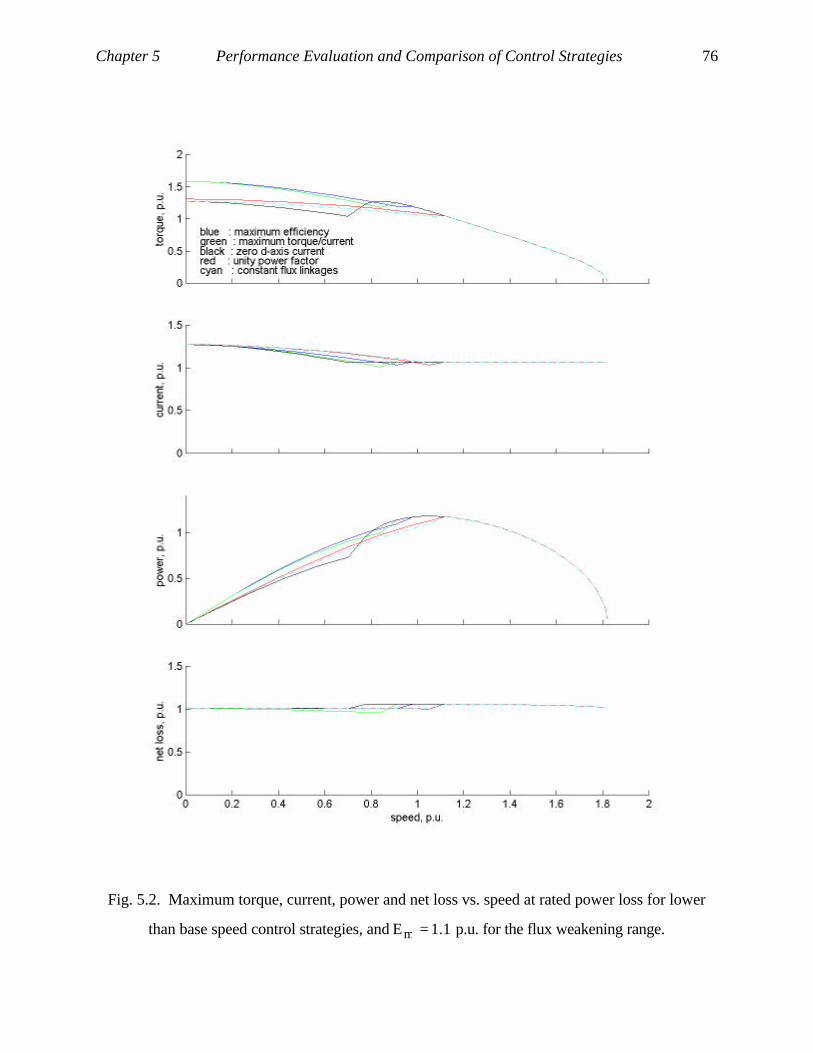
Chapter 5 Performance Evaluation and Comparison of Control Strategies
76
Fig. 5.2. Maximum torque, current, power and net loss vs. speed at rated power loss for lower
than base speed control strategies, and 1.1Em = p.u. for the flux weakening range.

Chapter 5 Performance Evaluation and Comparison of Control Strategies
77
Fig. 5.3. Torque per current, back emf, power factor and net loss vs. speed at rated power loss for
lower than base speed control strategies, and 1.1Em = p.u. for the flux weakening range.

Chapter 5 Performance Evaluation and Comparison of Control Strategies
78
The maximum torque for the ZDAC control strategy actually rises between the speeds of 0.7 and
0.9 p.u. speed. This is due to the introduction of non-zero d-axis current in the flux weakening
range, which produces reluctance torque.
B. Current vs. Speed
All control strategies require the same current at zero speed under the constant power loss
criteria. This is due to the fact that core losses are zero at zero speed. Therefore, constant net
power loss implies constant copper losses at zero speed. And, constant copper losses result in
identical current magnitude for all control strategies at zero speed. As speed increases the
current requirements of the five control strategies diverge significantly. The CMFL control
strategy has the highest current requirement. The rate of drop of current increases successively
for each of the UPF, ME, MTPC and ZDAC control strategies.
C. Power vs. Speed
The ME control strategy produces more power at any given speed than any other control
strategy. The power levels drops successively for each of the MTPC, UPF, CMFL and ZDAC
controls strategies.
D. Torque per Current vs. Speed
The ME and MTPC control strategies produce almost the same torque per current vs. speed
envelope. The ZDAC and CMFL control strategies result in roughly 1 p.u. torque per current for
the full range of speed. The toque per current envelope for the UPF control strategy is only
slightly higher than that of the CMFL control strategy.
E. Back EMF vs. Speed
The ZDAC control strategy results in the highest back emf among the five control strategies.
This, in turn, significantly limits the speed range before flux weakening for the ZDAC control
strategy. The UPF and CMFL control strategies result in the least back emf among the five
control strategies, and lower back emf requirements leads to increased speed range before flux
Chapter 5 Performance Evaluation and Comparison of Control Strategies
79
weakening for these two control strategies. The ME and MTPC control strategies also have
similar back emf requirements, and their back emf requirements are significantly higher than that
of UPF and CMFL control strategies.
F. Air gap Flux Linkages vs. Speed
Higher back emf at a given speed indicates higher mutual flux linkages as well. Therefore,
mutual flux linkages requirements can be studied using back emf vs. speed figures. The ZDAC
control strategy requires by far the highest air gap flux linkages of all control strategies at any
speed. This may raise concerns regarding saturation of the core for some machines. The ME
and MTPC control strategies both require roughly the same air gap flux linkages. The CMFL
and UPF control strategies require the least mutual flux linkages among all control strategies.
The CMFL and UPF control strategies both require roughly the same back emf. Therefore, the
flux linkages of the UPF control strategy is roughly 1 p.u., i.e. almost the same as that of the
CMFL control strategy.
G. Power Factor vs. Speed
The UPF control strategy results in the highest possible power factor of 1 for the full range of
speed. The CMFL control strategy results in a nearly unity power factor as well. The ZDAC
control strategy results in the worst power factor of all five control strategies. The power factor
is roughly 0.65 on the average in this case. The ME and MTPC control strategies both result in
reasonable power factors ranging from 0.85 at lower speeds to 0.95 at higher speeds. Power
factor increases for both of these control strategies as speed increases.
H. Speed Range Before Flux Weakening
The CMFL control strategy results in the widest speed range before flux weakening among the
five control strategies. The UPF control strategy stands with a slightly lower speed range. The
ZDAC control strategy yields the narrowest speed range. This is mainly due to the relatively
large air gap flux linkages for this control strategy. Note that the ZDAC control strategy is the
only control strategy where the magnet flux linkages is never opposed by a countering field in
the rotor’s d-axis. The speed ranges for the ME and MTPC control strategies fall in between that
Chapter 5 Performance Evaluation and Comparison of Control Strategies
80
of the ZDAC and UPF control strategies. The ME control strategy results in a slightly higher
speed range than the MTPC control strategy.
I. Base Speed
The speed at which the back emf reaches the maximum possible value along the maximum
torque vs. speed envelop is defined here as base speed. The base speed is a function of
maximum permissible power loss, maximum voltage available to the phase, and the choice of
control strategies. The specific objective of a control strategy in the lower than base speed
operating range cannot be met beyond the base speed along the operational envelope of the
system. It is seen that the CMFL control strategy provides the largest base speed among the five
control strategies. The base speed reduces successively for each of the UPF, MTPC, ME and
ZDAC control strategies.
J. Complexity of Implementation
The ZADC control strategy is the simplest as far as implementation is concerned. dI is simply
maintained at zero which makes the torque proportional to the phase current. The MTPC,
CMFL and UPF control strategies all require the implementation of separate functions for each
of the d and q axis currents. These currents are functions of torque only. Therefore,
implementation of the MTPC, CMFL and UPF control strategies involves the same level of
complexity. However, in the case of the ME control strategy the currents, qi and di , are
functions of both torque and speed. The necessary equations, in all cases, can be implemented
on-line, or by implementing look-up tables [44].
5.5.2 Higher than Base Speed Operating Range
In this section the two control strategies for the flux weakening range are compared in terms of
maximum torque vs. speed envelope, current requirements, base speed, maximum speed, current
and torque ripples, large signal torque response, and implementation complexity. The SSV
control strategy is shown to provide a significantly larger maximum torque vs. speed envelope
for operation under constant power loss. A larger operational envelope translates into a wider

Chapter 5 Performance Evaluation and Comparison of Control Strategies
81
speed range as well. The fundamental component of current in the case of SSV control strategy
is shown to be lower in magnitude than that of the CBE control strategy. It is also shown that the
application of the SSV control strategy results in a wider speed range below base speed before
flux weakening needs to be initiated. It is shown that the magnitude of the six-step current and
torque ripples are relatively low. The relatively low magnitude of ripple can be attributed to the
fact that in PMSM the phase self inductance limits the current ripple. It is shown that the SSV
control strategy is simpler to implement as it requires only position information contrary to the
CBE control strategy requiring in addition information on two phase currents. This increases the
sensor requirements for CBE control strategy compared to the SSV strategy.
A. Operational Boundary
Fig. 5.4 shows the operational boundary for the CBE control strategy with mE = 0.8 p.u., bus
voltage of 1.72 p.u., and rated total power loss for the motor drive as described in Appendix I.
The operational boundary for the SSV control strategy is also shown under the same conditions.
The voltage drop across the stator resistance is assumed to be negligible in this simulation. But,
stator resistance is taken into account in calculating power losses. It is seen that the operational
boundary for the SSV control strategy is significantly larger than that of the CBE control
strategy.
B. Base Speed
The starting point for the operational boundary for each control strategy in Fig. 5.4 is the base
speed for that control strategy. It is seen that the SSV control strategy provides a higher base
speed than that provided by the CBE control strategy. Therefore, the SSV control strategy
allows for a wider range of operation before flux weakening is initiated.
C. Maximum Speed in the Flux Weakening Range
As the maximum available voltage to the phase increases the maximum possible speed also
increases. The maximum speeds for the SSV and CBE control strategies are 4877 and 6374
RPM, respectively, as calculated from (5.28) for the example of Fig. 5.4.

Chapter 5 Performance Evaluation and Comparison of Control Strategies
82
p.u. ,Ten
p.u. ,Isn
p.u. ,Pln
SSV control strategy
SSV control strategy
100x torqueaverageripple torque
%
ripple torque.u.p
enω
p.u. 8.0Em =
SSV control strategy
CBE control strategy
Fig. 5.4. Maximum torque, peak current, net power loss, torque ripple as a percentage of average
torque, and peak to peak torque ripple for SSV (solid lines) and CBE (dashed lines, mE =0.8
p.u.) control strategies.
Chapter 5 Performance Evaluation and Comparison of Control Strategies
83
D. Maximum Current Requirements
It is shown in section 5.4.1 that the fundamental component of current is constant along the
operational boundary in the flux weakening range for both control strategies. The fundamental
voltage available to the phase is always higher in the case of the SSV control strategy.
Therefore, it can be concluded from (5.36) that the fundamental component of current is always
lower in the case of the SSV control strategy. Maintaining the back emf at a lower value than
mV requires a significant d-axis current to oppose the magnet flux linkages. This results in a
higher stator current for the CBE control strategy. This additional current does not contribute
proportionally to torque development.
The drive must be able to provide the peak current for any control strategy. The peak current
for the SSV control strategy is different from the fundamental component of current. This is due
to presence of significant current ripple. Fig. 5.4 shows the peak current along the operational
boundary for the SSV control strategy. It is seen that in the worst case the peak value is about
10% higher than the fundamental value of 1.1 p.u. This brings the peak current requirement of
the SSV control strategy to approximately 1.2 p.u. for the given example. A realistic comparison
on the basis of current requirements must compare the peak current in the case of SSV control
strategy to the fundamental current for the CBE control strategy. Fig. 5.4 shows that the
fundamental component of current under the CBE control strategy is slightly over 1.2 p.u. for a
desired back emf of 0.8 p.u. It is seen that in this example the current requirements of both
control strategies are in the same order. However, if the desired back emf can be increased
above 0.8 p.u., then the current in the CBE control strategy drops below the peak current in the
SSV control strategy.
E. Torque Ripple
The torque ripple, resulting from the application of the CBE control strategy, is caused by the
PWM or hysteresis current control system. The impact of this torque ripple on system
performance is negligible as compared to the torque ripple inherent to the SSV control strategy.
Chapter 5 Performance Evaluation and Comparison of Control Strategies
84
Fig. 5.4 shows the peak to peak torque pulsation as a percentage of average torque along the
maximum torque vs. speed envelope for the SSV control strategy. It is seen that the peak to peak
torque pulsation remains within 7 to 20 percent of the average torque along the operational
boundary. But, it is noted that in absolute normalized unit, the torque pulsation is less than 0.1
p.u. at all speeds.
F. Large Signal Torque Response
The CBE control strategy provides a faster torque response as compared to the SSV control
strategy. This is due to the availability of a voltage margin in the CBE control strategy.
Simulation results for the motor drive described in Appendix I show that the CBE control
strategy with a 10 volts margin at a DC bus voltage of 57 V at 1500 RPM results in a time
response of 8 ms for a –1 to 1 N.m. step torque command. The SSV control strategy results in a
20 ms time response for the same transition.
G. Complexity of Implementation
The SSV control strategy is easier to implement than the CBE control strategy. Only one
lookup table is required to provide the angle of voltage phasor as a function of torque command
and speed. However, in the case of the CBE control strategy, one look-up table is required for
each of q and d-axis current commands as a function of torque command and speed. Also, the
CBE control strategy requires current feedbacks in addition to rotor position feedback.
However, the SSV control strategy only requires rotor position feedback. The switching losses
of the drive under the SSV control strategy are much less than that resulting from the CBE
control strategy. This is due to the fact that the switching frequency for the SSV control strategy
is much lower than that of the CBE control strategy.
5.6 PERFORMANCE COMPARISON INSIDE THE OPERATIONAL ENVELOPE
In the last section the performances of different control strategies along their respective
operational envelope are studied. However, for a given control strategy, and at a given speed,
the torque command may be anywhere between zero and maximum possible torque at that speed.
In this section the performance of different control strategies are compared as a function of
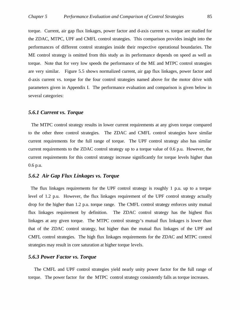
Chapter 5 Performance Evaluation and Comparison of Control Strategies
85
torque. Current, air gap flux linkages, power factor and d-axis current vs. torque are studied for
the ZDAC, MTPC, UPF and CMFL control strategies. This comparison provides insight into the
performances of different control strategies inside their respective operational boundaries. The
ME control strategy is omitted from this study as its performance depends on speed as well as
torque. Note that for very low speeds the performance of the ME and MTPC control strategies
are very similar. Figure 5.5 shows normalized current, air gap flux linkages, power factor and
d-axis current vs. torque for the four control strategies named above for the motor drive with
parameters given in Appendix I. The performance evaluation and comparison is given below in
several categories:
5.6.1 Current vs. Torque
The MTPC control strategy results in lower current requirements at any given torque compared
to the other three control strategies. The ZDAC and CMFL control strategies have similar
current requirements for the full range of torque. The UPF control strategy also has similar
current requirements to the ZDAC control strategy up to a torque value of 0.6 p.u. However, the
current requirements for this control strategy increase significantly for torque levels higher than
0.6 p.u.
5.6.2 Air Gap Flux Linkages vs. Torque
The flux linkages requirements for the UPF control strategy is roughly 1 p.u. up to a torque
level of 1.2 p.u. However, the flux linkages requirement of the UPF control strategy actually
drop for the higher than 1.2 p.u. torque range. The CMFL control strategy enforces unity mutual
flux linkages requirement by definition. The ZDAC control strategy has the highest flux
linkages at any given torque. The MTPC control strategy’s mutual flux linkages is lower than
that of the ZDAC control strategy, but higher than the mutual flux linkages of the UPF and
CMFL control strategies. The high flux linkages requirements for the ZDAC and MTPC control
strategies may result in core saturation at higher torque levels.
5.6.3 Power Factor vs. Torque
The CMFL and UPF control strategies yield nearly unity power factor for the full range of
torque. The power factor for the MTPC control strategy consistently falls as torque increases.
Chapter 5 Performance Evaluation and Comparison of Control Strategies
86
Fig. 5.5. Current, air gap flux linkages, power factor and d-axis current vs. torque for different
control strategies.

Chapter 5 Performance Evaluation and Comparison of Control Strategies
87
However, its power factor remains above the reasonable value of 0.8 for the full range of torque.
The power factor for the ZDAC control strategy falls significantly as torque command increases.
5.6.4 D-axis Current vs. Torque
The ZDAC control strategy enforces zero d-axis current on the motor. All the other control
strategies require an increasing magnitude of negative d-axis current as torque increases. The d-
axis current requirement of the UPF and CMFL control strategies are similar and relatively
significant. The MTPC control strategy requires reasonable d-axis current for the full range of
torque. High levels of d-axis current can demagnetize the magnets.
5.6.5 Torque Range
The UPF control strategy has the smallest torque range among the four control strategies. This
is due to the fact that beyond a certain torque the power factor cannot be maintained at 1 as
discussed in section 5.3.4. The other control strategies do not have any absolute torque limit
within the shown range. However, both air gap flux and d-axis current limitations can impose
torque limits on these control strategies depending on the structure of the motor. The air gap flux
linkages is limited primarily by magnetic saturation. Therefore, application of the ZDAC control
strategy may result in a torque limit because of its relatively high air gap flux linkages
requirements. Similarly, the maximum possible d-axis current imposes torque limitations on the
UPF and CMFL control strategies due to their relatively high d-axis current requirements.
5.7 DIRECT STEADY STATE EVALUATION IN SSV MODE
In this section the boundary matching technique is utilized in finding the instantaneous q and d
axis current waveforms in steady state for a PMSM operating in the SSV mode.
Assuming that the angle of the voltage phasor with reference to the rotor’s d-axis is α then the
q and d-axis voltages can be described in rotor reference frame as,
)3/tcos(V32
)t(v rdcqs α−π+ω= 3/t0 r π<ω≤ (5.37)

Chapter 5 Performance Evaluation and Comparison of Control Strategies
88
)3/tsin(V32
)t(v rdcds α−π+ω= 3/t0 r π<ω≤ (5.38)
The same pattern repeats in the 3/2t3 r π<ω≤π period as well as other periods. Note that α is
the independent control variable that can be used to control average torque. The fundamental
components of (5.37) and (5.38) are the same as the values given by (5.30) and (5.31),
respectively, for a given α . The periodic voltage inputs, as described by (5.37) and (5.38), result
in periodic q and d axis currents. The periodicity and continuity of the currents are exploited
here to derive the waveforms of qi and di for one period of 3/π radians. The PMSM equations
in rotor reference frame are written in state variable form as,
eBUBXAX 111111 ++=& (5.39)
where
tdq1 ]ii[X = , 1
11 PQA −= , 1
1 QB −= , tdsqs1 ]vv[u = ,
tafr ]0 [e λω−= ,
=
d
qL00L
Q ,
−ωω−−
=sqr
drs1 RL
LRP
Equations (5.37) and (5.38) can be described in differential format as given below,
2ds
qs
r
r2
.
ds.
qs.
SXv
v
0
0X
v
v=
ω
ω−==
(5.40)
where the dot on top of the variables denotes differentiation with respect to time. Considering
only the part without rotor flux induced emf in the q axis, equations (5.39) and (5.40) are
combined to yield,
AXX.
= , [ ] t21 XXX = ,
=
S0BA
A 11 (5.41)
The solution of (5.41) is written as,
Chapter 5 Performance Evaluation and Comparison of Control Strategies
89
)0(Xe)t(X At= r3
t0ωπ
<≤ (5.42)
The initial condition vector is given below,
tdsqsdq )]0( v)0( v)0(i )0(i[)0(X = (5.43)
where )0(X is to be evaluated to compute X(t). X(0) is found using the fact that the state vector
has periodic symmetry and hence,
)0(XS)3
(X 1r
=ωπ
(5.44)
where 1S is evaluated later. The boundary condition for the currents are,
)0(X)3
(X 1r
1 =ωπ
(5.45)
The boundary matching condition for the voltage vector is obtained by expanding (5.37) and
(5.38).
)0(v23
)0(v21
3sin)
3sin(
3cos)
3cos(V
32
)33
cos(V32
)3
(v
dsqs
dc
dcr
qs
−=
π
α−π
−π
α−π
=
π+α−
π=
ωπ
(5.46)
Similarly,
)0(v21
)0(v23
)3
(v dsqsr
ds +=ωπ
(5.47)
Hence
)0(XS)0(X
21
23
23
21
3X 222
r2 =
−
=
ωπ (5.48)

Chapter 5 Performance Evaluation and Comparison of Control Strategies
90
Substituting equation (5.45) and (5.48) into (5.42),
)0(Xe)0(XS00I
)0(XS3
X r3A
21
r
ωπ
=
==
ωπ (5.49)
where I is a 2x2 identity matrix. Hence,
0)0(WX)0(X]eS[ r3A
1 ==−
ωπ
(5.50)
where,
=−=
ωπ
43
213A
1 WWWW
]eS[W r (5.51)
where 1W , 2W , 3W and 4W are 22 × matrices. Expanding the upper row in (5.50), gives the
following relationship,
0)0(XW)0(XW 2211 =+ (5.52)
from which the steady state current vector )0(X1 is obtained as,
)0(XWW)0(X 221
11−−= (5.53)
Having evaluated the initial current vector, it could be used to evaluate currents for one full cycle
and the electromagnetic torque. Now using (5.42) the exact current vector as a function of angle
can be derived for one period, starting at t = 0, as,
I
I)0(Xe
0 0 1 00 0 0 1
)t(i
)t(i
d
qAt
d
q
+
=
(5.54)
Chapter 5 Performance Evaluation and Comparison of Control Strategies
91
where tdq ]I I[ is the steady state response due to the induced emf by the rotor flux linkages.
As the induced emf is a constant at a given speed, its response in the machine has to also be a
constant in steady state. Hence the d and q axes current derivatives are zero. With that the
steady state currents are,
[ ]t
qd2r
2s
afq2r
qd2r
2s
safrt
dq LLR
L,
LLR
RI,I
ω+
λω−
ω+
λω−= (5.55)
5.8 SIMULATION AND EXPERIMENTAL VERIFICATION
Experimental correlation is provided using a prototype motor drive utilizing an interior PMSM
with parameters given in Appendix I. The experimental PMSM motor drive is set up as a torque
controller for the higher than base speed operating range. An 8 kByte EEPROM is utilized as a
lookup table with torque command and measured speed as its inputs in order to implement the
SSV control strategy. The output of this EEPROM is the angle of voltage phasor. One 8 kByte
EEPROM lookup table is utilized for each of the q and d axis current commands in order to
implement the CBE control strategy. Both q and d-axis current commands are functions of
measured speed and torque commands for the CBE control strategy. Fig. 5.6 shows the
estimated and measured maximum possible torque vs. speed for the CBE and SSV control
strategies. The maximum power loss is set at 30 W in both cases, and the bus voltage is 65 V.
The constant back emf is 33 V for the CBE control strategy leaving a margin of 8 V between the
back emf and the peak of the fundamental voltage available to each phase. The stator voltage
phasor required to maintain the back emf at 33 V is enforced using the SSV control setup by pre-
calculating the required stator voltage phasor on a point by point basis. It is clearly seen that at
any speed the maximum possible torque is much higher for the SSV control strategy. The
measured maximum speeds for the SSV and CBE control strategies are approximately 1900
RPM and 1650 RPM, respectively. These speed limits correlate closely to the calculated values
of 2000 RPM and 1634 RPM, respectively, using (5.28).
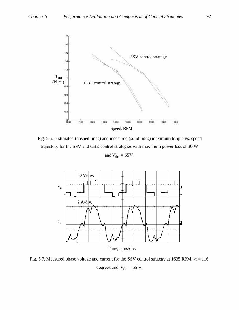
Chapter 5 Performance Evaluation and Comparison of Control Strategies
92
emT
CBE control strategy
Speed, RPM
SSV control strategy
.)m.N(
Fig. 5.6. Estimated (dashed lines) and measured (solid lines) maximum torque vs. speed
trajectory for the SSV and CBE control strategies with maximum power loss of 30 W
and .V65Vdc =
Time, 5 ms/div.
av
ai
50 V/div.
2 A/div.
Fig. 5.7. Measured phase voltage and current for the SSV control strategy at 1635 RPM, 116=α
degrees and =dcV 65 V.
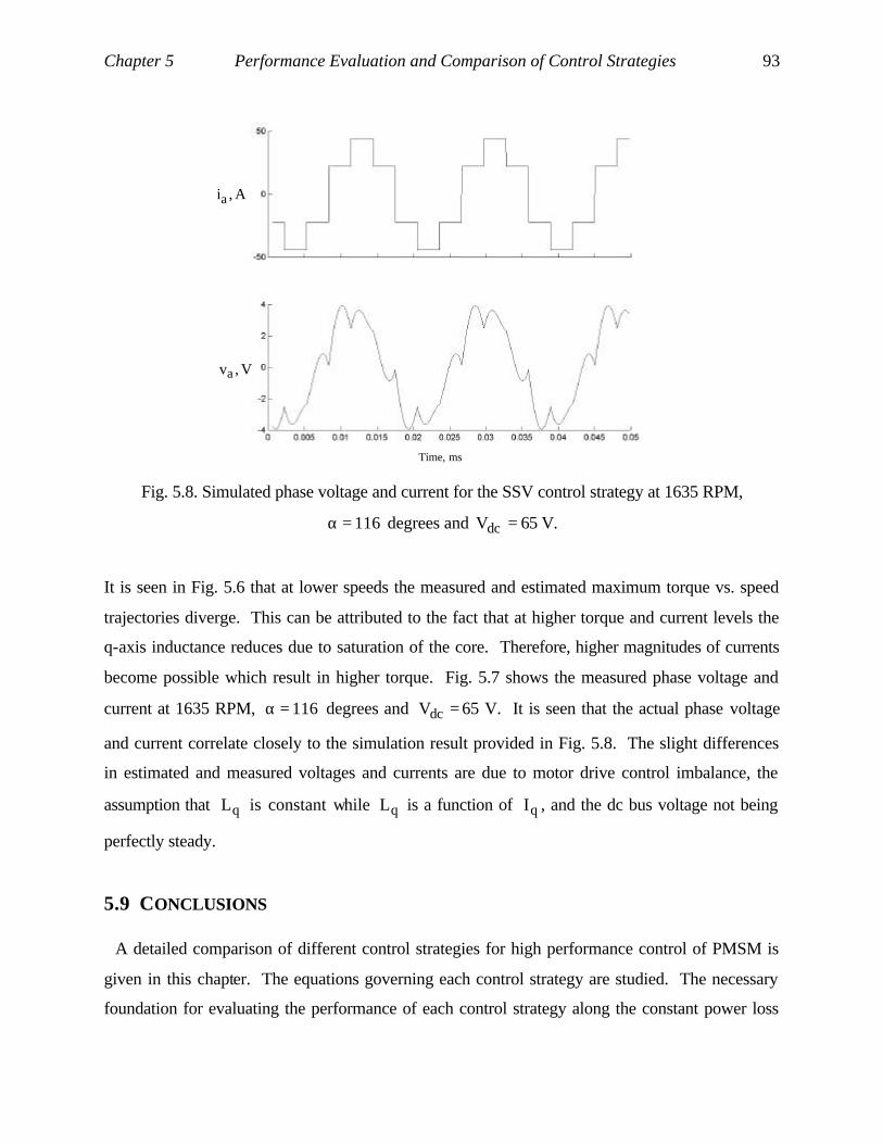
Chapter 5 Performance Evaluation and Comparison of Control Strategies
93
A ,ia
V ,va
Time, ms Fig. 5.8. Simulated phase voltage and current for the SSV control strategy at 1635 RPM,
116=α degrees and =dcV 65 V.
It is seen in Fig. 5.6 that at lower speeds the measured and estimated maximum torque vs. speed
trajectories diverge. This can be attributed to the fact that at higher torque and current levels the
q-axis inductance reduces due to saturation of the core. Therefore, higher magnitudes of currents
become possible which result in higher torque. Fig. 5.7 shows the measured phase voltage and
current at 1635 RPM, 116=α degrees and =dcV 65 V. It is seen that the actual phase voltage
and current correlate closely to the simulation result provided in Fig. 5.8. The slight differences
in estimated and measured voltages and currents are due to motor drive control imbalance, the
assumption that qL is constant while qL is a function of qI , and the dc bus voltage not being
perfectly steady.
5.9 CONCLUSIONS
A detailed comparison of different control strategies for high performance control of PMSM is
given in this chapter. The equations governing each control strategy are studied. The necessary
foundation for evaluating the performance of each control strategy along the constant power loss

Chapter 5 Performance Evaluation and Comparison of Control Strategies
94
operating envelope is laid out. All control strategies are compared based on their performances
along the constant power loss operational envelope as well as their performances inside the
envelope. The procedures provided in this study can be used to choose the control strategy that
optimizes the motor drive system based on the requirements of a particular application.
The contributions of this chapter are summarized below:
• Performance analysis of different control strategies for PMSM along the constant power loss
operational envelope
• Comparison of control strategies along the constant power loss operating envelope
• Comparison of control strategies inside the operating envelope
• Derivation of absolute maximum torque for the unity power factor and constant mutual flux
linkages control strategies
• Derivation of maximum speed, current and torque in the flux weakening range as a function
of maximum power loss and machine parameters.
• Experimental verification of key results

95
CHAPTER 6
Analysis and Implementation of Concurrent Mutual
Flux Weakening and Torque Control for PMSM
6.1 INTRODUCTION
Concurrent mutual flux linkages and torque control is necessary for the high performance
control of PMSM in the higher than base speed operating range. Implementing such a system
involves the solution of a fourth order polynomial. The parameters of this polynomial depend on
rotor speed, commanded mutual flux linkages and torque as well as machine parameters.
Implementing a fourth order polynomial equation solver is a difficult task, and requires
expensive processors. Two practical implementation strategies are discussed in this chapter.
The first one is based on a lookup table approach. The two-dimensional lookup tables are
prepared offline, and then implemented within a high performance motor drive. It is shown that
the implementation of the lookup tables is relatively straightforward. Dynamic simulation shows
that the lookup table approach results in very high accuracy of control. However,
implementation of the lookup tables requires a significant amount of programmable memory.
An alternative implementation strategy is to replace the lookup tables with polynomials fits.
This approach results in far less memory requirements, but introduces more error and results in a
slower system. A procedure for replacing the polynomials with artificial neural networks is
suggested later in Chapter 7. The maximum possible torque as a function of the desired mutual
flux linkages is studied in this chapter.
The contributions of this chapter are summarized below:
• Introduction of two practical implementation schemes, based on lookup tables or
equations, for the concurrent flux linkages weakening and torque control for PMSM
• Comparison of the two implementation schemes
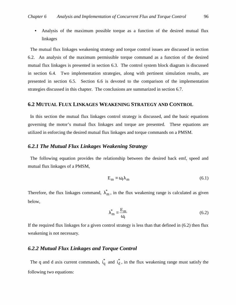
Chapter 6 Analysis and Implementation of Concurrent Flux and Torque Control 96
• Analysis of the maximum possible torque as a function of the desired mutual flux
linkages
The mutual flux linkages weakening strategy and torque control issues are discussed in section
6.2. An analysis of the maximum permissible torque command as a function of the desired
mutual flux linkages is presented in section 6.3. The control system block diagram is discussed
in section 6.4. Two implementation strategies, along with pertinent simulation results, are
presented in section 6.5. Section 6.6 is devoted to the comparison of the implementation
strategies discussed in this chapter. The conclusions are summarized in section 6.7.
6.2 MUTUAL FLUX LINKAGES WEAKENING STRATEGY AND CONTROL
In this section the mutual flux linkages control strategy is discussed, and the basic equations
governing the motor’s mutual flux linkages and torque are presented. These equations are
utilized in enforcing the desired mutual flux linkages and torque commands on a PMSM.
6.2.1 The Mutual Flux Linkages Weakening Strategy
The following equation provides the relationship between the desired back emf, speed and
mutual flux linkages of a PMSM,
mrmE λω= (6.1)
Therefore, the flux linkages command, *mλ , in the flux weakening range is calculated as given
below,
r
m*m
Eω
=λ (6.2)
If the required flux linkages for a given control strategy is less than that defined in (6.2) then flux
weakening is not necessary.
6.2.2 Mutual Flux Linkages and Torque Control
The q and d axis current commands, *qi and *
di , in the flux weakening range must satisfy the
following two equations:
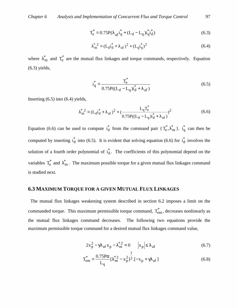
Chapter 6 Analysis and Implementation of Concurrent Flux and Torque Control 97
)ii)LL(i(P75.0T *d
*qqd
*qaf
*e −+λ= (6.3)
2*qq
2af
*dd
2*m )iL()iL( +λ+=λ (6.4)
where *mλ and *
eT are the mutual flux linkages and torque commands, respectively. Equation
(6.3) yields,
)i)LL((P75.0
Ti
af*dqd
*e*
qλ+−
= (6.5)
Inserting (6.5) into (6.4) yields,
2
af*dqd
*eq2
af*dd
2*m )
)i)LL((P75.0
TL()iL(
λ+−+λ+=λ (6.6)
Equation (6.6) can be used to compute *di from the command pair *
m*e ,T λ . *
qi can then be
computed by inserting *di into (6.5). It is evident that solving equation (6.6) for *
di involves the
solution of a fourth order polynomial of *di . The coefficients of this polynomial depend on the
variables *eT and *
mλ . The maximum possible torque for a given mutual flux linkages command
is studied next.
6.3 MAXIMUM TORQUE FOR A GIVEN MUTUAL FLUX LINKAGES
The mutual flux linkages weakening system described in section 6.2 imposes a limit on the
commanded torque. This maximum permissible torque command, *emT , decreases nonlinearly as
the mutual flux linkages command decreases. The following two equations provide the
maximum permissible torque command for a desired mutual flux linkages command value,
x0xx2 afp2*
mpaf2p λ≤=λ−γλ− (6.7)
]x.[]x[L
P75.0T afp
2
12p
2*m
q
*em γλ+−−λα= (6.8)
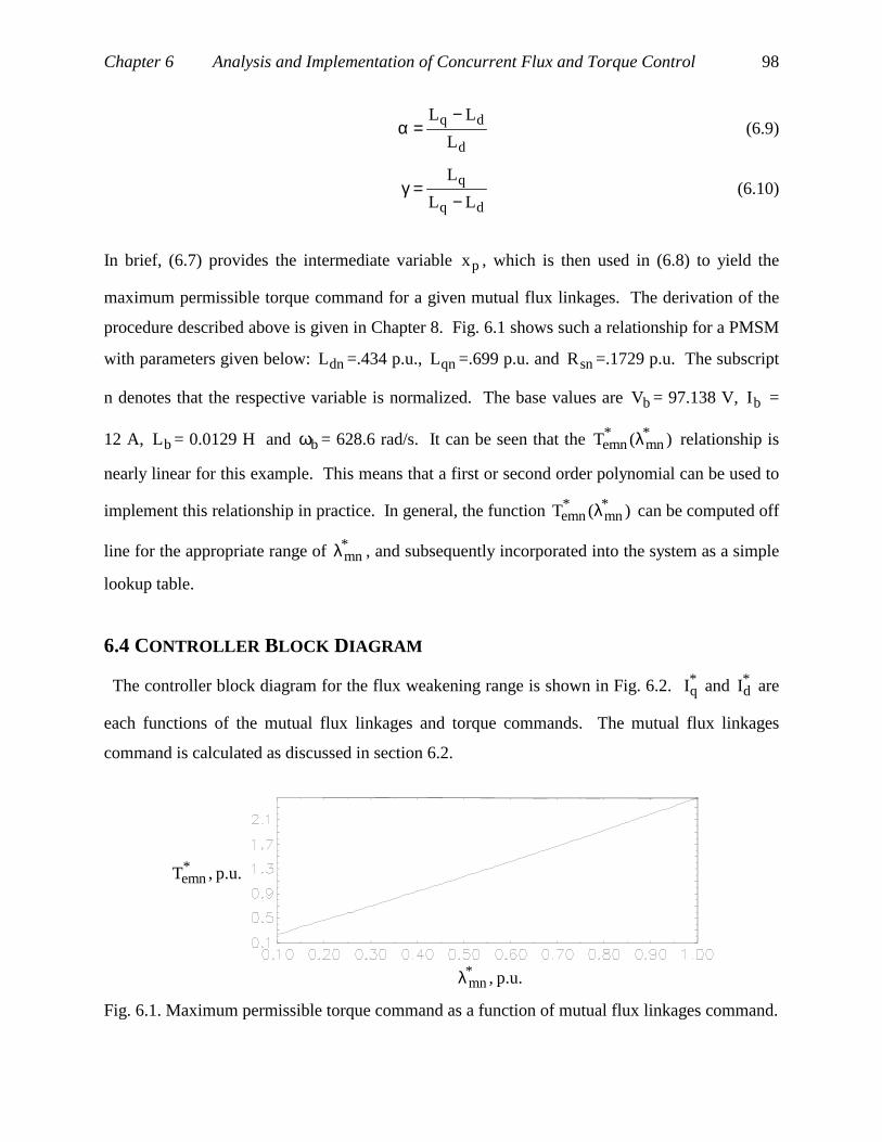
Chapter 6 Analysis and Implementation of Concurrent Flux and Torque Control 98
d
dq
L
LL −=α (6.9)
dq
q
LL
L
−=γ (6.10)
In brief, (6.7) provides the intermediate variable px , which is then used in (6.8) to yield the
maximum permissible torque command for a given mutual flux linkages. The derivation of the
procedure described above is given in Chapter 8. Fig. 6.1 shows such a relationship for a PMSM
with parameters given below: dnL =.434 p.u., qnL =.699 p.u. and snR =.1729 p.u. The subscript
n denotes that the respective variable is normalized. The base values are bV = 97.138 V, bI =
12 A, bL = 0.0129 H and bω = 628.6 rad/s. It can be seen that the )(T *mn
*emn λ relationship is
nearly linear for this example. This means that a first or second order polynomial can be used to
implement this relationship in practice. In general, the function )(T *mn
*emn λ can be computed off
line for the appropriate range of *mnλ , and subsequently incorporated into the system as a simple
lookup table.
6.4 CONTROLLER BLOCK DIAGRAM
The controller block diagram for the flux weakening range is shown in Fig. 6.2. *qI and *
dI are
each functions of the mutual flux linkages and torque commands. The mutual flux linkages
command is calculated as discussed in section 6.2.
p.u.,T*emn
p.u.,*mnλ
Fig. 6.1. Maximum permissible torque command as a function of mutual flux linkages command.

Chapter 6 Analysis and Implementation of Concurrent Flux and Torque Control 99
*eT Lookup tables
orequations
r
mE
ω *mλ
rω
*qsiConversion
matrix *dsi
*qi
rω*di
Fig. 6.2. Controller block diagram for the flux weakening range.
The torque command and measured speed are the inputs to this system. The torque command,
*eT , may be an independent variable, or it may be the output of a proportional-integrator
controller acting on the difference between the commanded and measured speeds. The mutual
flux linkages command is calculated as discussed in section 6.2. Either lookup tables or
equations can be used to calculate the d and q axis current commands as a function of the mutual
flux linkages and torque commands. The stator current commands, *dsi and *
qsi , are calculated as
a function of *qi , *
di and rω as shown in the conversion matrix (6.11). This conversion matrix
increases the control accuracy by taking core losses into account. Implementation of (6.11) is
highly recommended at higher speeds. The stator current commands are enforced on the motor
using an appropriate current controller.
ωλ+
ω−
ω
=
0
Ri
i
1R
L
R
L1
i
ic
raf
*d
*q
c
rq
c
rd
*ds
*qs
(6.11)
The controller block diagram for the lower than base speed operating range is shown in Fig.
6.3.
*eT Lookup tables
orequationsrω
*qsiConversion
matrix *dsi
*qi
rω*di
Fig. 6.3. Controller block diagram for the lower than base speed operating range.
Chapter 6 Analysis and Implementation of Concurrent Flux and Torque Control 100
The lower than base speed operating range is initiated only if,
r
mm
E
ω<λ (6.12)
where mλ is the required flux linkages. *qi and *
di are each functions of the torque command
and speed in the most general case. Any of the control strategies discussed in section 3 of
Chapter 5 can be implemented as lookup tables or equations in this case. *qsi and *
dsi are
calculated as a function of *qi , *
di and rω as shown in (6.11).
6.5 IMPLEMENTATION STRATEGIES
Two alternative implementation strategies for the concurrent control of mutual flux linkages
and torque are presented in this section. Implementation of either of the two is simpler than the
on-line solution of a fourth order equation described in section 6.2.
6.5.1 Lookup Table Approach
In this section the lookup table implementation strategy for the on-line computation of *q
*d i,i
from *m
*e ,T λ is discussed. All implementation strategies follow the following general format,
Ω=*di ),T( *
m*
e λ (6.13)
Λ=i*q ),T( *m
*e λ (6.14)
where Ω and Λ represent the relationships described in (6.3) and (6.4). The lookup table
approach is illustrated here through an example using the parameters of a PMSM described in
section 6.3.
Equations (6.13) and (6.14) can be realized using separate two-dimensional lookup tables.
These lookup tables are generated off line by numerically solving equations (6.3) and (6.4). The
two independent axes of each table are assigned to *eT and *
mλ , respectively. The respective

Chapter 6 Analysis and Implementation of Concurrent Flux and Torque Control 101
values of *di or *
qi is read inside each table. Note that the tables need only provide the data for
positive torque commands. For negative torque commands the q-axis current command from the
table must be applied with negative sign. *mλ is limited to values between 0 and base value
since the only interest is in weakening the mutual flux linkages. The numerical solution to
equations (6.3) and (6.4) for the motor parameters given in section 6.3, and for the following
range of normalized mutual flux linkages command,
12.0 *mn ≤λ≤ , p.u. (6.15)
yields the operating ranges for the other three variables as
44.2T0 *en ≤≤ , p.u. (6.16)
3.3i0 *dn ≤≤ , p.u. (6.17)
3.3i0 *qn ≤≤ , p.u. (6.18)
Figures 6.4 and 6.5 show the two-dimensional tables for this system. In practice the variables
are digitized under the following constraints in order to reduce storage requirements,
:T*en 9 bits (6.19)
:*mnλ 7 bits (6.20)
*dni and *
qni : 8 bits each (6.21)
Once the torque command reaches its maximum permissible value, the current commands are
frozen. The fact that each graph has two distinct areas is due to this restriction. In each graph,
the border between these two surfaces appears to be a straight line, which can be attributed to the
fact that the )(T *mn
*emn λ relationship is nearly linear for this example. The )(T *
mn*emn λ
relationship, shown in Fig. 6.1, suggests that for the given parameters, the relationship can be
adequately approximated with a first or second order polynomial. Thus, any of the following
two polynomials can be used for the on line calculation of *emnT from *
mnλ in this example. The
polynomials are both derived using the least squares fit method.

Chapter 6 Analysis and Implementation of Concurrent Flux and Torque Control 102
p.u.,*mnλ
p.u.,T*en
p.u.,i*qn
Fig. 6.4. *qni as a function of normalized mutual flux linkages and torque commands.
p.u.,*mnλ
p.u.,T*en
p.u.,i*dn
Fig. 6.5. *dni as a function of normalized mutual flux linkages and torque commands.
0059.23.221.0T *mn
2*mn
*emn +λ+λ= (6.22)
or simply,
*mn
*emn 44.2T λ= (6.23)
Utilization of these tables results in accurate enforcement of the commanded torque and the
commanded mutual flux linkages. Fig. 6.6 shows simulation results for a speed control system
that utilizes the two tables shown above for a speed controlled operation with +3 p.u. and -3 p.u.

Chapter 6 Analysis and Implementation of Concurrent Flux and Torque Control 103
speed commands. The mutual flux linkages is maintained at rated value until the phase voltage
requirement reaches 0.53 p.u. at which point flux weakening is initiated. The stator resistance is
taken into account in the simulation, and this is why the mutual flux weakening is initiated at a
speed of 0.53 p.u. instead of 1 p.u. The torque command is the difference between the
commanded and actual speeds multiplied by a factor of 100. The dotted lines represent
commanded values and solid lines represent actual values. The PWM is operating at 20 kHz and
the current error is amplified by a factor of 200. Due to the limited bandwidth of the current
controller, the ability of the system to enforce the desired currents decreases as speed increases.
As a consequence the mutual flux linkages error increases with speed. It is seen from Fig. 6.6
that the mutual flux linkages and torque commands are enforced accurately. Figure 6 in Chapter
7 is similar to Fig. 6.6, but it also provides the phase voltage and actual and commanded q and d-
axis currents. Note that memory chips are required to store the relatively large look-up tables.
Each table has 162 entries, and each entry is digitized using 8 bits. Therefore, each table
requires 64 kilobytes of storage capacity. This can be considered as a tradeoff for achieving
accurate control over the machine’s mutual flux linkages and torque.
6.5.2 Two-Dimensional Polynomials Approach
An alternative to the lookup table approach is to approximate the tables using two-dimensional
polynomials. In this case equations (6.13) and (6.14) are implemented as,
)(a+...T).(ai *mn0
r*en
*mnr
*dn λ+λ= (6.24)
)(b+...T).(bi *mn0
r*en
*mnr
*qn λ+λ= (6.25)
where,
i0s*
mnsi*mni x+....x)(a +λ=λ (6.26)
i0s*
mnsi*mni y+....y)(b +λ=λ (6.27)
and r is the order of the polynomials that are used to compute *dni and *
qni using equations (6.24)
and (6.25), and s is the order of the polynomials that are used to compute the coefficients of
(6.26) and (6.27).

Chapter 6 Analysis and Implementation of Concurrent Flux and Torque Control 104
Time, s
p.u.,*mnλ
p.u.,mnλ
p.u.,T*en
p.u.,T*en
p.u.,*rnω
p.u.,rnω
Fig. 6.6. Normalized speed, torque, mutual flux linkages for a ± 3 p.u. step speed command.
The appropriate order for each polynomial must be chosen on a case by case basis. Obviously,
higher order polynomials provide a better fit at the expense of increased implementation
complexity. The unknown coefficients can be identified for a given PMSM using least squares
fits. The two-dimensional polynomial approach does not have any significant memory storage
requirements. However, the advantage of not having to store large tables comes at a tradeoff for
mutual flux linkages and torque enforcement accuracy. Fig. 6.7 shows the achieved and
commanded mutual flux linkages for various mutual flux linkages and torque command values
for the motor parameters presented earlier. Polynomials of 3rd and 5th order are used for the
main and coefficient equations, respectively. It can be seen that in the worst case the mutual flux
linkages error goes up to ten percent.

Chapter 6 Analysis and Implementation of Concurrent Flux and Torque Control 105
p.u.,T*en
p.u.,*mnλ
p.u.,mnλ
Fig. 6.7. Commanded and achieved mutual flux linkages vs. commanded torque for the
polynomial implementation approach.
The digitized values of the mutual flux linkages and torque commands can be used in the
implementation of equations (6.24) to (6.27). The higher than 1 powers of these variables, in
digital values, can be computed off line and stored in tables. These tables can later be utilized, at
the implementation level, to readily provide the higher powers of the variables instead of
performing time consuming multiplications. Assuming that *enT and *
mnλ are digitized using 8
bits, storing the higher powers of each variable requires 256x(2+3+...+ η ) bytes, where η is the
highest order of the respective variable. For the example provided in this section, η is equal to 3
for the main equations and 5 for the coefficient equations. Therefore, the memory required to
store the two tables is approximately 5 kilobytes. On the other hand, 16 multiplications and 16
additions are required to implement equations (6.24) to (6.27) for the case given in this example.
6.6 COMPARISON OF THE TWO APPROACHES
The lookup table approach provides a high level of accuracy in terms of enforcing the mutual
flux linkages and torque commands as compared to the two-dimensional polynomial approach.
Therefore, utilizing lookup tables results in meeting the specified voltage requirements of the
drive system, which is one of the key factors in the drive’s performance. The system is also
relatively fast since implementing it mainly involves reading data from a memory chip, and the
performance of minimal calculations. However, implementing this system requires a

Chapter 6 Analysis and Implementation of Concurrent Flux and Torque Control 106
considerable amount of digital memory capacity. For the example provided in this section 128
kilobytes of ROM is required to store the tables. The two-dimensional polynomial fit approach
provides an alternative to the former approach. It resolves the problem of large memory
requirements. Roughly 5 kilobytes of memory is required for the implementation scheme
presented in section 6.5. However, this system introduces a significant amount of error in terms
of enforcing the desired mutual flux linkages and torque. The error is more pronounced at higher
levels of mutual flux linkages and torque commands as seen from Fig. 6.7. The system is also
inherently more complicated to implement than the lookup table approach since it requires the
implementation of variable coefficient polynomials. Moreover, the computation of the command
values using two-dimensional polynomials slows down the system due to the numerous
multiplications that have to be performed. Other sources of error that are common to both
approaches are the digitization of the variables, limited bandwidth of the current controller, and
parameter variations.
6.7 CONCLUSIONS
Two practical implementation schemes are formulated, analyzed and verified by dynamic
simulation for the concurrent mutual flux linkages weakening and torque control of a PMSM.
The most straight forward scheme is to use lookup tables, which provides a high level of
accuracy. As a tradeoff, the method requires additional memory chips to be present on board to
store the tables. In another approach these lookup tables are approximated using two-
dimensional polynomials. The two-dimensional polynomial approximation method introduces
error in terms of achieving the desired mutual flux linkages and torque. The maximum
permissible torque command as a function of the mutual flux linkages command is studied, and
methods for taking this restriction into account are discussed. The maximum permissible torque
command decreases nonlinearly as the mutual flux linkages is weakened.
The contributions of this chapter are summarized below:
• Introduction of practical implementation schemes, based on lookup tables or equations,
for the concurrent mutual flux linkages weakening and torque control for PMSM
• Comparison of the two implementation schemes
• Analysis of the maximum possible torque as a function of mutual flux linkages
107
CHAPTER 7
Concurrent Mutual Flux Weakening and Torque
Control in the Presence of Parameter Variations
7.1 INTRODUCTION
It is shown in Chapter 6 that the q and d axis current commands can be implemented using two-
dimensional lookup tables or equations in order to enforce a desired mutual flux linkages and
torque command on a PMSM. The two-dimensional tables are prepared off-line using the
nominal parameters of the machine. However, some of the machine parameters deviate from
their nominal values during normal operation of the machine. These variations are due to
changes in temperature as well as magnetic saturation of the core, and result in mutual flux
linkages and torque enforcement error. The mutual flux linkages error may directly translate into
higher voltage requirements. The torque error results in a nonlinear torque response of the
system. The computation of the correct current commands involves the on-line solution of a
fourth order polynomial equation as discussed in Chapter 6. The coefficients of this polynomial
depend on machine parameters as well as the commanded values for mutual flux linkages and
torque. Theoretically, this fourth order polynomial can be solved on-line while its parameters are
calculated based on estimated values of machine parameters. However, this method is not
feasible for practical applications due to its intensive computational requirements. It is shown in
this chapter that lookup tables can be prepared offline to yield an offset for the current commands
in response to the variation of a desired parameter. Each of the final current commands in this
case is the sum of a nominal value and an offset. The nominal value is calculated based on the
nominal values of machine parameters. The offset is function of the estimated value of a specific
parameter as well as the mutual flux linkages and torque commands. The application of the
nominal current vector, along with the computed offset, results in greatly reduced errors in
mutual flux linkages and torque command enforcement. This is true for the full range of mutual
Chapter 7 Concurrent Flux Weakening and Torque Control With Parameter Variations 108
flux linkages control, and hence, for a wide range of operating speed. A large number of lookup
tables are required in order to accurately cover the full range of the varying parameter. An
alternative approach is to train neural networks to replace the tables. Simulation results show
that neural networks are well suited for this purpose. A comparison between the two approaches
is made in this chapter. The magnet flux linkages is the most critical parameter to be
compensated for in PMSM drives, and, therefore, it is used in most of this chapter's examples.
Other parameters can be treated in a similar way.
The contributions of this chapter are summarized below:
• Procedure for computing the current vector compensation offset using lookup tables
• Procedure for computing the current vector compensation offset using neural networks
• Comparison of the two approaches
The nature of the variations of different PMSM parameters is discussed in section 7.2. The
impact of parameter variations on mutual flux linkages and torque enforcement is studied in
section 7.3. The parameter compensation scheme, along with two implementation strategies, are
discussed in section 7.4. A comparison of the two implementation strategies is given in section
7.5. Dynamic simulation of a neural network based compensator is presented in section 7.6. The
procedures for estimating the q-axis inductance and rotor flux linkages are discussed in section
7.7. The conclusions are summarized in section 7.8.
7.2 THE VARIATION OF PARAMETERS IN PMSM
The stator resistance, rotor flux linkages and q-axis inductance are the only parameters of a
PMSM that vary significantly. The variation of the stator resistance does not have any material
impact on the operation of high performance PMSM drives. This is due to the fact that high
performance PMSM drives predominantly use current controllers that enforce a desired current
on the motor regardless of the value of stator resistance. The torque of a PMSM depends on the
q and d-axis inductances and currents as well as the rotor flux linkages. Also note that the
voltage drop across the phase resistance is generally small compared to the back emf in the flux

Chapter 7 Concurrent Flux Weakening and Torque Control With Parameter Variations 109
weakening range for most PMSM. The rotor flux linkages may decrease by as much as 20%
while the motor is running under normal operating conditions depending on the magnets used.
The residual rotor flux linkages declines as the temperature of the magnets rise. The q-axis
inductance decreases as the q-axis current increases. The q-axis path of some types of PMSM has
a relatively low reluctance which results in saturation of the path as q-axis current increases.
This is especially true for inset and interior PMSM which have low reluctance along their q-axis
paths. The saturation of the q-axis path results in declining q-axis inductance. The q-axis
inductance of such motors may vary by as much as 20% of its nominal value. The surface mount
PMSM is effectively immune to inductance variations due to the large effective air gap which
results in relatively high reluctance along both d and q axes.
7.3 THE IMPACT OF PARAMETER VARIATIONS
The mutual flux linkages and torque controller system is shown in Fig. 7.1.
Lookup Tablesor
Equations
PMSM
Drive SystemMotor
*eT
*mλ
*qi
*di
rθ
c,b,ai eT
mλ
Fig. 7.1. The mutual flux linkages and torque control system.
*mλ and *
eT are the mutual flux linkages and torque commands, respectively. *eT can be an
independent command value, or it may be the output of a controller acting on the difference
between the commanded and measured values of speed. *qi and *
di are the q and d-axis current
commands, respectively. The difference between stator and rotor current commands, which is
due to core losses, is ignored here; but this difference can be accounted for by utilizing the
conversion matrix given in (6.11). The current commands are calculated using lookup tables or
equations that are prepared offline using nominal parameters of the specific PMSM. The

Chapter 7 Concurrent Flux Weakening and Torque Control With Parameter Variations 110
measured values of the a, b and c phase currents, c,b,ai , are used by the PMSM drive system to
control current. The rotor angle, rθ , is used by the drive system to implement vector control.
mλ and eT are the actual mutual flux linkages and torque, respectively. The mutual flux
linkages and torque commands are achieved accurately as long as the actual and nominal
parameters of the machine match. The sources of error in this case are mainly digitization error
and current enforcement error due to the limited bandwidth of the current controller. In practice,
motor parameters vary depending on the operating conditions of the machine. These variations
cause a mismatch between the actual and commanded values of mutual flux linkages and torque.
The mutual flux linkages and torque errors, mλ∆ and eT∆ , respectively, are defined as,
m*mm λ−λ=λ∆ (7.1)
e*ee TTT −=∆ (7.2)
The variations of both afλ and qL have a direct impact on the system as described in Fig. 7.1,
and can cause significant errors in mutual flux linkages and torque. The equations relating the
mutual flux linkages and torque to the q and d-axis currents are given below,
2qq
2afdd
2m )iL()iL( +λ+=λ (7.3)
)ii)LL(i(P75.0T dqqdqafe −+λ= (7.4)
Figures 7.2 and 7.3 show the normalized values of mλ∆ and eT∆ as a function of the mutual
flux linkages and torque commands for a 20% drop in the rotor flux linkages for the system
shown in Fig. 7.1. The parameters of the PMSM used in this study are given in section 3 of
Chapter 6. It can be seen that the mutual flux linkages and torque errors are as much as 0.2 and
0.3 p.u., respectively. For the case where the actual and nominal parameters are identical, the
mutual flux linkages and torque errors are negligible due to the accuracy of the nominal tables.
The rotor flux linkages and q-axis compensation procedures are discussed in the next section.

Chapter 7 Concurrent Flux Weakening and Torque Control With Parameter Variations 111
p.u.,*mnλ
p.u.,T*en
p.u.,Ten∆
Fig. 7.2. Normalized torque error when p.u.8.0af =λ
p.u.,*mnλ
p.u.,T*en
p.u.,mnλ∆
Fig. 7.3. Mutual flux linkages error when p.u.8.0af =λ
7.4 PARAMETER COMPENSATION SCHEME
The direct calculation of the current commands from (7.3) and (7.4) involves the on-line
solution of a fourth order polynomial of di as explained in Chapter 6. The parameters of this
polynomial depend on the commanded values and machine parameters, and must also be
estimated on-line. The on-line solution of this polynomial results in a theoretically perfect
system assuming that accurate estimations of the respective parameters are utilized. However,
the method is not feasible for practical applications due to its intensive computational
requirements. A feasible alternative is to compute parameter-dependent offsets to be added to
the nominal current commands. The command offsets, which are computed on-line, compensate
for the effects of parameter variations. Fig. 7.4 gives a block diagram of this system.
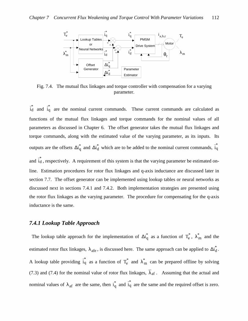
Chapter 7 Concurrent Flux Weakening and Torque Control With Parameter Variations 112
Lookup Tables
or
Neural Networks
PMSM
Drive SystemMotor
OffsetGenerator
*eT
*mλ
*qi
*di
*qi
*di
++
++
Parameter
Estimator
eT
mλrθ
*qi∆*di∆
c,b,ai
Fig. 7.4. The mutual flux linkages and torque controller with compensation for a varyingparameter.
*di and
*qi are the nominal current commands. These current commands are calculated as
functions of the mutual flux linkages and torque commands for the nominal values of all
parameters as discussed in Chapter 6. The offset generator takes the mutual flux linkages and
torque commands, along with the estimated value of the varying parameter, as its inputs. Its
outputs are the offsets *qi∆ and *
di∆ which are to be added to the nominal current commands,*qi
and*di , respectively. A requirement of this system is that the varying parameter be estimated on-
line. Estimation procedures for rotor flux linkages and q-axis inductance are discussed later in
section 7.7. The offset generator can be implemented using lookup tables or neural networks as
discussed next in sections 7.4.1 and 7.4.2. Both implementation strategies are presented using
the rotor flux linkages as the varying parameter. The procedure for compensating for the q-axis
inductance is the same.
7.4.1 Lookup Table Approach
The lookup table approach for the implementation of *qi∆ as a function of *
eT , *mλ and the
estimated rotor flux linkages, afeλ , is discussed here. The same approach can be applied to *di∆ .
A lookup table providing*qi as a function of *
eT and *mλ can be prepared offline by solving
(7.3) and (7.4) for the nominal value of rotor flux linkages, afλ . Assuming that the actual and
nominal values of afλ are the same, then *qi and
*qi are the same and the required offset is zero.
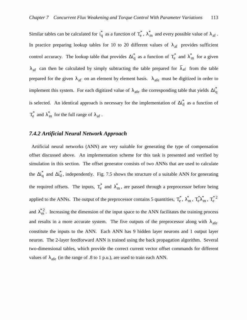
Chapter 7 Concurrent Flux Weakening and Torque Control With Parameter Variations 113
Similar tables can be calculated for *qi as a function of *
eT , *mλ and every possible value of afλ .
In practice preparing lookup tables for 10 to 20 different values of afλ provides sufficient
control accuracy. The lookup table that provides *qi∆ as a function of *
eT and *mλ for a given
afλ can then be calculated by simply subtracting the table prepared for afλ from the table
prepared for the given afλ on an element by element basis. afeλ must be digitized in order to
implement this system. For each digitized value of afeλ the corresponding table that yields *qi∆
is selected. An identical approach is necessary for the implementation of *di∆ as a function of
*eT and *
mλ for the full range of afλ .
7.4.2 Artificial Neural Network Approach
Artificial neural networks (ANN) are very suitable for generating the type of compensation
offset discussed above. An implementation scheme for this task is presented and verified by
simulation in this section. The offset generator consists of two ANNs that are used to calculate
the *qi∆ and *
di∆ , independently. Fig. 7.5 shows the structure of a suitable ANN for generating
the required offsets. The inputs, *eT and *
mλ , are passed through a preprocessor before being
applied to the ANNs. The output of the preprocessor contains 5 quantities, *eT , *
mλ , *m
*eT λ , 2*
eT
and 2*mλ . Increasing the dimension of the input space to the ANN facilitates the training process
and results in a more accurate system. The five outputs of the preprocessor along with afeλ
constitute the inputs to the ANN. Each ANN has 9 hidden layer neurons and 1 output layer
neuron. The 2-layer feedforward ANN is trained using the back propagation algorithm. Several
two-dimensional tables, which provide the correct current vector offset commands for different
values of afeλ (in the range of .8 to 1 p.u.), are used to train each ANN.

Chapter 7 Concurrent Flux Weakening and Torque Control With Parameter Variations 114
Preprocessor
9 Neuron Hidden Layer
Single neuronoutput layer
Two-layerFeedforward
Network
or
afeλ *eT *
mλ
*di∆ *
qi∆
Fig. 7.5. The ANN based offset generator structure.
7.5 COMPARISON OF THE TWO APPROACHES
It is important to notice that the lookup table approach results in the most accurate
implementation scheme for the offset generators. The lookup tables represent accurate solutions
to the equations discussed earlier. On the other hand, neural networks are trained to mimic the
behavior of the tables, and therefore, cannot represent the tables accurately. However, as is
shown later in section 7.6, neural networks exhibit a sufficient capacity in replacing the lookup
tables in high performance motor drive applications. The lookup table approach provides an
inherently faster system as compared to the neural network approach. No multiplications are
required with lookup tables. However, 108 multiplications are required just to implement the
weights in two separate ANNs as shown in Fig. 7.5. Therefore, the timing requirements become
more stringent due to the increased demand on sequential software operations. Also, the
nonlinear activation functions must be implemented using additional lookup tables or using
dedicated integrated circuits. The main disadvantage of using lookup tables is the relatively
large amount of programmable memory required by the system. Two tables are required for each
digitized value of afeλ . Therefore, 128 Kb of memory is required to implement the offset tables
required for each digitized value of afeλ . This is based on 9 bit digitization for torque, and 7 bit

Chapter 7 Concurrent Flux Weakening and Torque Control With Parameter Variations 115
digitization for mutual flux linkages. Therefore, 4 bit digitization of afeλ necessitates 2
megabytes of programmable memory in addition to the 128 kb memory requirements of the
nominal command tables.
7.6 DYNAMIC SIMULATION
Fig. 7.6 shows simulation results for a speed control system that utilizes the neural network
approach discussed in section 7.4.2 for the concurrent control of mutual flux linkages and torque.
The torque command is the difference between the commanded and actual speeds multiplied by a
factor of 100. The mutual flux linkages is maintained at rated value until the phase voltage
requirement reaches 1 p.u. at which point flux weakening is initiated. The dotted lines in Fig. 7.6
represent command values and solid lines represent actual values. The speed commands are ± 3
p.u. The rotor flux linkages is assumed to have dropped 20 percent below its nominal value.
Mutual flux linkages weakening is initiated at a speed of 0.6 p.u. Neural networks are used to
provide both the nominal q and d-axis current commands and their respective offsets. The phase
current commands are enforced using a PWM system operating at 20 kHz with a gain of 300. It
can be seen that the mutual flux linkages and torque commands are enforced with high accuracy
for the full range of speed while the voltage requirements never exceed 1 p.u. This simulation
shows that artificial neural networks can be effectively utilized in implementing parameter
insensitive controllers for PMSM. In an independent set of simulations, the ANNs are trained to
compensate for the q-axis self inductance variations. Fig. 7.7 shows the respective simulation
results for the case where qL is 20% lower than its nominal value.

Chapter 7 Concurrent Flux Weakening and Torque Control With Parameter Variations 116
p.u.,*mnλ
p.u.,mnλ
p.u.,Vsn
p.u.,T*en
p.u.,T*en
p.u.,i,i qn*qn
p.u.,i,i dn*dn
p.u.,*rnω
p.u.,rnω
Time, s
Fig. 7.6. Commanded and actual values for speed, torque, mutual flux linkages, q and d-axiscurrents and phase voltage for a ± 3 p.u. speed command in the presence of 20 percent reduction
in rotor flux linkages.
.
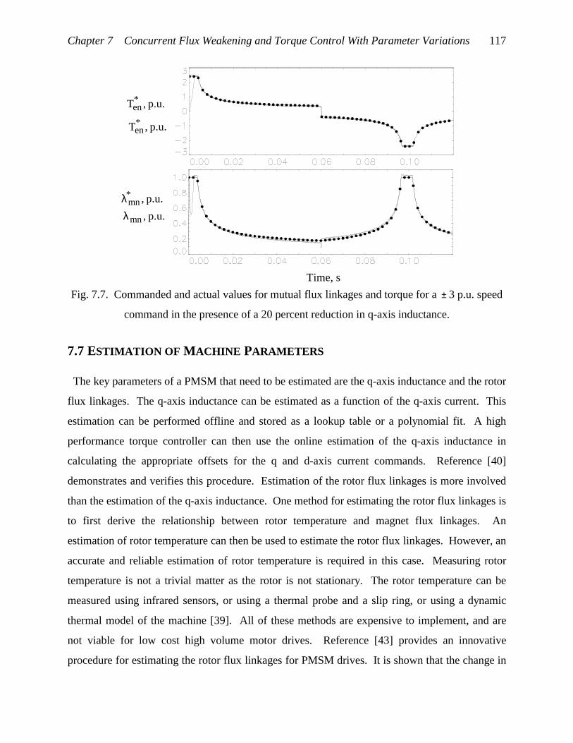
Chapter 7 Concurrent Flux Weakening and Torque Control With Parameter Variations 117
p.u.,*mnλ
p.u.,mnλ
p.u.,T*en
p.u.,T*en
Time, s
Fig. 7.7. Commanded and actual values for mutual flux linkages and torque for a ± 3 p.u. speed
command in the presence of a 20 percent reduction in q-axis inductance.
7.7 ESTIMATION OF MACHINE PARAMETERS
The key parameters of a PMSM that need to be estimated are the q-axis inductance and the rotor
flux linkages. The q-axis inductance can be estimated as a function of the q-axis current. This
estimation can be performed offline and stored as a lookup table or a polynomial fit. A high
performance torque controller can then use the online estimation of the q-axis inductance in
calculating the appropriate offsets for the q and d-axis current commands. Reference [40]
demonstrates and verifies this procedure. Estimation of the rotor flux linkages is more involved
than the estimation of the q-axis inductance. One method for estimating the rotor flux linkages is
to first derive the relationship between rotor temperature and magnet flux linkages. An
estimation of rotor temperature can then be used to estimate the rotor flux linkages. However, an
accurate and reliable estimation of rotor temperature is required in this case. Measuring rotor
temperature is not a trivial matter as the rotor is not stationary. The rotor temperature can be
measured using infrared sensors, or using a thermal probe and a slip ring, or using a dynamic
thermal model of the machine [39]. All of these methods are expensive to implement, and are
not viable for low cost high volume motor drives. Reference [43] provides an innovative
procedure for estimating the rotor flux linkages for PMSM drives. It is shown that the change in

Chapter 7 Concurrent Flux Weakening and Torque Control With Parameter Variations 118
the rotor flux linkages is equal to the change in reactive power divided by speed and d-axis
current. The reactive power can be estimated using the d and q-axis currents and voltages. The
strength of this procedure is that the variations in stator resistance do not affect the estimation of
the rotor flux linkages. This procedure can only be applied to PMSM drives that utilize non-zero
d-axis current in their torque control strategy.
7.8 CONCLUSIONS
A procedure for the concurrent mutual flux weakening and torque control of PMSM in the
presence of parameter variations is introduced in this chapter. The procedure is based on an
offset generator for the q and d-axis current commands. The required offsets are calculated as a
function of mutual flux linkages and torque commands as well as an on-line estimation of a
varying PMSM parameter. Two implementation strategies based on lookup tables and neural
networks are presented and compared based on their respective implementation requirements. It
is shown that the lookup table approach results in a fast and accurate system, but requires a
significant amount of programmable memory. The neural network approach is shown to result in
a high level of accuracy without requiring much programmable memory. However, the neural
network approach results in an inherently slower system due to the large number of calculations
that need to be performed on-line. The results are verified by simulations of the systems.
In general, it can be concluded that artificial neural networks exhibit a sufficient capacity in
replacing the lookup tables in high performance motor drive applications.
The contributions of this chapter are summarized below:
• Procedure for computing the current vector compensation offset using lookup tables
• Procedure for computing the current vector compensation offset using neural networks
• Comparison of the two approaches

119
CHAPTER 8
Applications of a New Normalization Technique
8.1 INTRODUCTION
A new normalization technique is introduced in this chapter. This normalization technique is
particularly useful in the analysis and simulation of PMSM motor drives. The magnet flux
linkages and d-axis inductance are used as normalization bases. Therefore, these parameters, as
well as number of poles, are eliminated from all equations. This greatly simplifies the analysis
and simulation of PMSM motor drive performance. The standard normalization technique uses
the rated values of variables as its bases. Another innovative normalization technique, which
also results is simplified equations, has been introduced in [31]. A comparison of the new
normalization technique with the other two techniques shows the superiority of the former.
Several key derivations are presented in this chapter using the new normalization technique. It is
clearly seen that the elimination of two parameters from all equations results in analytical terms
that are easier to deduce, comprehend and simulate. However, the non-normalized form is the
preferred choice for demonstration purposes as it facilitates the understanding of the impact of
each parameter on system performance. Also, it is preferred to normalize the variables in all
plots using rated values of variables in order to make the plots easier to understand and study.
One of the applications of the new normalization technique is in the preparation of generalized
application characteristics. For example current and power factor vs. torque characteristics for
different control strategies depend only on the saliency ratio when these characteristics are
normalized using the new normalization technique.
The contributions of this chapter are summarized below:
• Introduction of a new normalization technique
• Derivation of the maximum torque vs. speed envelopes for the ME, MTPC, ZDAC, CMFL,
UPF, CBE control strategies operating with constant power loss

Chapter 8 Applications of a New Normalization Technique 120
• Derivation of the maximum continuous current requirement of a PMSM drive operating with
constant power loss
• Derivation of the maximum possible torque for a given mutual flux linkages
• Introduction of generalized application characteristics for PMSM drives
Section 8.2 describes the details of the new normalization technique. This technique is
compared to two other normalization techniques in section 8.3. The maximum torque vs. speed
envelope for six different control strategies is derived in section 8.4. The maximum current
requirement of the drive is derived in section 8.5. The maximum possible torque for a given
mutual flux linkages is calculated in section 8.6. Section 8.7 introduces generalized application
characteristics for PMSM using the new normalization technique. The conclusions are presented
in section 8.8.
8.2 THE NEW NORMALIZATION TECHNIQUE
The base values for this normalization technique are given below:
db LL = (8.1)
afb λ=λ (8.2)
rrb ω=ω (8.3)
where bL , bλ and bω are the base values for the d-axis inductance, magnet flux linkages and
electrical speed, respectively, and rrω is the rated value for the rotor's electrical speed. The base
values chosen in (8.1) and (8.2) are chosen to eliminate dL and afλ from all equations. This
results in significant simplification of all equations as is demonstrated below. The rated values
for torque and current are not 1 p.u. in this normalization technique, but rated speed is always 1
p.u. The base values for key variables of a PMSM can be calculated from (8.1) to (8.3) as,
d
afb L
Iλ
= (8.4)
afrbV λω= (8.5)
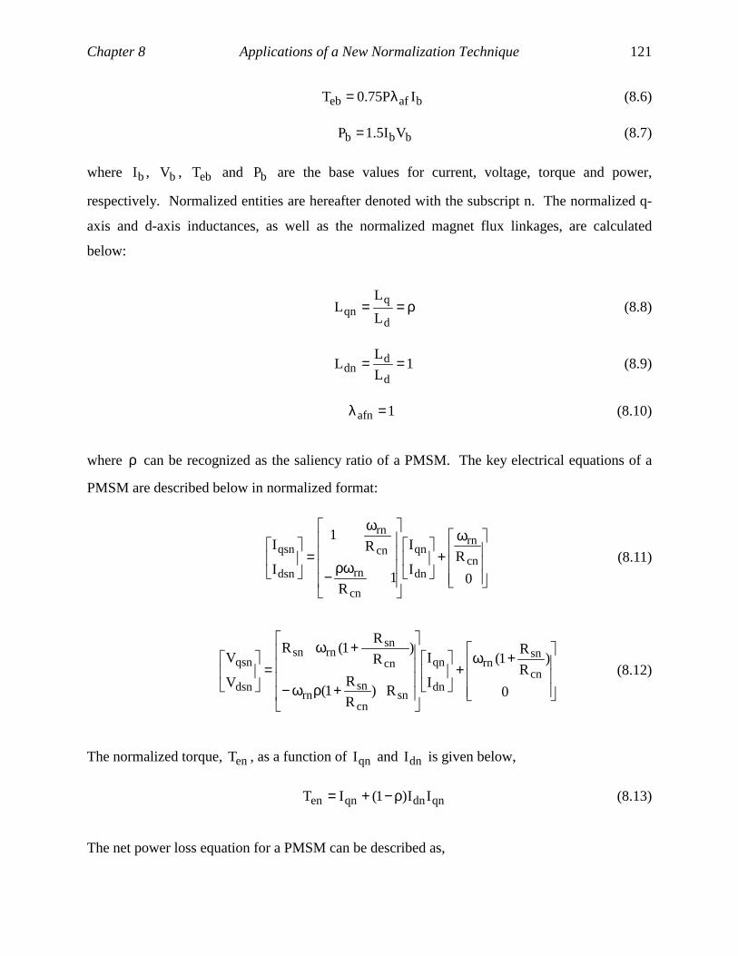
Chapter 8 Applications of a New Normalization Technique 121
bafeb IP75.0T λ= (8.6)
bbb VI5.1P = (8.7)
where bI , bV , ebT and bP are the base values for current, voltage, torque and power,
respectively. Normalized entities are hereafter denoted with the subscript n. The normalized q-
axis and d-axis inductances, as well as the normalized magnet flux linkages, are calculated
below:
ρ==d
qqn L
LL (8.8)
1L
LL
d
ddn == (8.9)
1afn =λ (8.10)
where ρ can be recognized as the saliency ratio of a PMSM. The key electrical equations of a
PMSM are described below in normalized format:
ω+
ρω−
ω
=
0
RI
I
1R
R1
I
Icn
rn
dn
qn
cn
rn
cn
rn
dsn
qsn(8.11)
+ω+
+ρω−
+ω=
0
)R
R1(
I
I
R)R
R1(
)R
R1(R
V
Vcn
snrn
dn
qn
sncn
snrn
cn
snrnsn
dsn
qsn(8.12)
The normalized torque, enT , as a function of qnI and dnI is given below,
qndnqnen II)1(IT ρ−+= (8.13)
The net power loss equation for a PMSM can be described as,
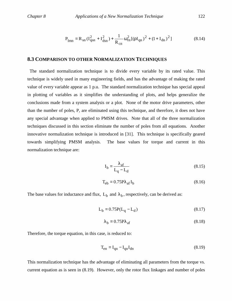
Chapter 8 Applications of a New Normalization Technique 122
])I1()I[(R
1)II(RP 2
dn2
qn2rn
cn
2dsn
2qsnsnlmn ++ρω++= (8.14)
8.3 COMPARISON TO OTHER NORMALIZATION TECHNIQUES
The standard normalization technique is to divide every variable by its rated value. This
technique is widely used in many engineering fields, and has the advantage of making the rated
value of every variable appear as 1 p.u. The standard normalization technique has special appeal
in plotting of variables as it simplifies the understanding of plots, and helps generalize the
conclusions made from a system analysis or a plot. None of the motor drive parameters, other
than the number of poles, P, are eliminated using this technique, and therefore, it does not have
any special advantage when applied to PMSM drives. Note that all of the three normalization
techniques discussed in this section eliminate the number of poles from all equations. Another
innovative normalization technique is introduced in [31]. This technique is specifically geared
towards simplifying PMSM analysis. The base values for torque and current in this
normalization technique are:
dq
afb LL
I−
λ= (8.15)
bafeb IP75.0T λ= (8.16)
The base values for inductance and flux, bL and bλ , respectively, can be derived as:
)LL(P75.0L dqb −= (8.17)
afb P75.0 λ=λ (8.18)
Therefore, the torque equation, in this case, is reduced to:
dnqnqnen IIIT −= (8.19)
This normalization technique has the advantage of eliminating all parameters from the torque vs.
current equation as is seen in (8.19). However, only the rotor flux linkages and number of poles
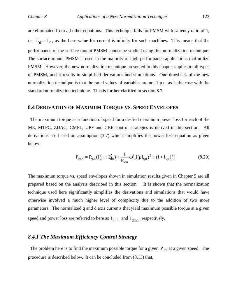
Chapter 8 Applications of a New Normalization Technique 123
are eliminated from all other equations. This technique fails for PMSM with saliency ratio of 1,
i.e. qd LL = , as the base value for current is infinity for such machines. This means that the
performance of the surface mount PMSM cannot be studied using this normalization technique.
The surface mount PMSM is used in the majority of high performance applications that utilize
PMSM. However, the new normalization technique presented in this chapter applies to all types
of PMSM, and it results in simplified derivations and simulations. One drawback of the new
normalization technique is that the rated values of variables are not 1 p.u. as is the case with the
standard normalization technique. This is further clarified in section 8.7.
8.4 DERIVATION OF MAXIMUM TORQUE VS. SPEED ENVELOPES
The maximum torque as a function of speed for a desired maximum power loss for each of the
ME, MTPC, ZDAC, CMFL, UPF and CBE control strategies is derived in this section. All
derivations are based on assumption (3.7) which simplifies the power loss equation as given
below:
])I1()I[(R
1)II(RP 2
dn2
qn2rn
cn
2dn
2qnsnlmn ++ρω++= (8.20)
The maximum torque vs. speed envelopes shown in simulation results given in Chapter 5 are all
prepared based on the analysis described in this section. It is shown that the normalization
technique used here significantly simplifies the derivations and simulations that would have
otherwise involved a much higher level of complexity due to the addition of two more
parameters. The normalized q and d axis currents that yield maximum possible torque at a given
speed and power loss are referred to here as qmnI and dmnI , respectively.
8.4.1 The Maximum Efficiency Control Strategy
The problem here is to find the maximum possible torque for a given lmP at a given speed. The
procedure is described below. It can be concluded from (8.13) that,
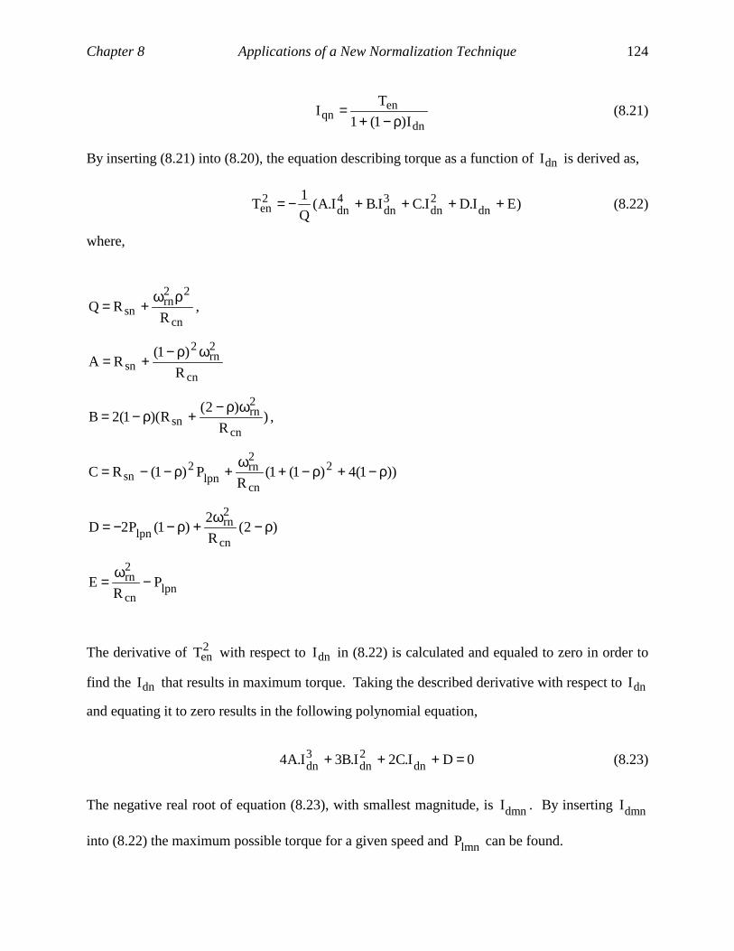
Chapter 8 Applications of a New Normalization Technique 124
dn
enqn I)1(1
TI
ρ−+= (8.21)
By inserting (8.21) into (8.20), the equation describing torque as a function of dnI is derived as,
)EI.DI.CI.BI.A(Q
1T dn
2dn
3dn
4dn
2en ++++−= (8.22)
where,
cn
22rn
sn RRQ
ρω+= ,
cn
2rn
2
sn R
)1(RA
ωρ−+=
)R
)2(R)(1(2B
cn
2rn
snωρ−
+ρ−= ,
))1(4)1(1(R
P)1(RC 2
cn
2rn
lpn2
sn ρ−+ρ−+ω
+ρ−−=
)2(R
2)1(P2D
cn
2rn
lpn ρ−ω
+ρ−−=
lpncn
2rn P
RE −
ω=
The derivative of 2enT with respect to dnI in (8.22) is calculated and equaled to zero in order to
find the dnI that results in maximum torque. Taking the described derivative with respect to dnI
and equating it to zero results in the following polynomial equation,
0DI.C2I.B3I.A4 dn2dn
3dn =+++ (8.23)
The negative real root of equation (8.23), with smallest magnitude, is dmnI . By inserting dmnI
into (8.22) the maximum possible torque for a given speed and lmnP can be found.
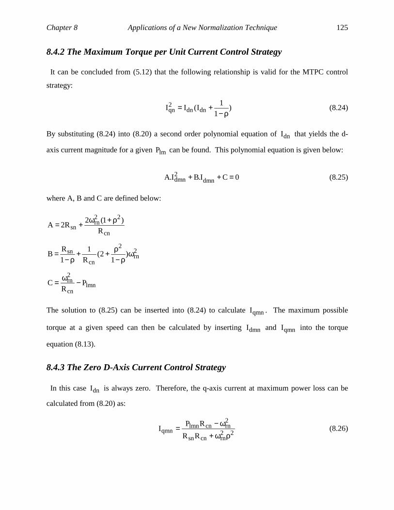
Chapter 8 Applications of a New Normalization Technique 125
8.4.2 The Maximum Torque per Unit Current Control Strategy
It can be concluded from (5.12) that the following relationship is valid for the MTPC control
strategy:
)1
1I(II dndn
2qn ρ−
+= (8.24)
By substituting (8.24) into (8.20) a second order polynomial equation of dnI that yields the d-
axis current magnitude for a given lmP can be found. This polynomial equation is given below:
0CI.BI.A dmn2dmn =++ (8.25)
where A, B and C are defined below:
cn
22rn
sn R)1(2
2RAρ+ω+=
2rn
2
cn
sn )1
2(R
11
RB ω
ρ−ρ++
ρ−=
lmncn
2rn P
RC −ω=
The solution to (8.25) can be inserted into (8.24) to calculate qmnI . The maximum possible
torque at a given speed can then be calculated by inserting dmnI and qmnI into the torque
equation (8.13).
8.4.3 The Zero D-Axis Current Control Strategy
In this case dnI is always zero. Therefore, the q-axis current at maximum power loss can be
calculated from (8.20) as:
22rncnsn
2rncnlmn
qmnRR
RPI
ρω+ω−= (8.26)
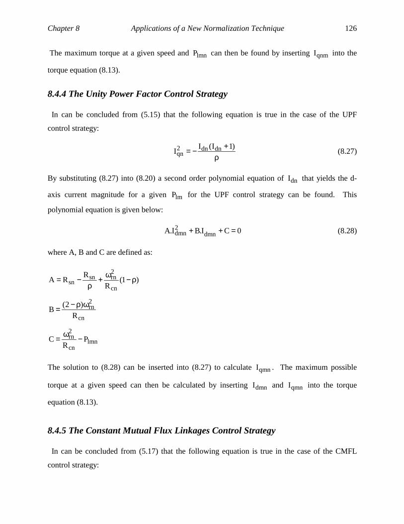
Chapter 8 Applications of a New Normalization Technique 126
The maximum torque at a given speed and lmnP can then be found by inserting qnmI into the
torque equation (8.13).
8.4.4 The Unity Power Factor Control Strategy
In can be concluded from (5.15) that the following equation is true in the case of the UPF
control strategy:
ρ+−= )1I(I
I dndn2qn (8.27)
By substituting (8.27) into (8.20) a second order polynomial equation of dnI that yields the d-
axis current magnitude for a given lmP for the UPF control strategy can be found. This
polynomial equation is given below:
0CI.BI.A dmn2dmn =++ (8.28)
where A, B and C are defined as:
)1(R
RRA
cn
2rnsn
sn ρ−ω+ρ
−=
cn
2rn
R)2(
Bωρ−=
lmncn
2rn P
RC −ω=
The solution to (8.28) can be inserted into (8.27) to calculate qmnI . The maximum possible
torque at a given speed can then be calculated by inserting dmnI and qmnI into the torque
equation (8.13).
8.4.5 The Constant Mutual Flux Linkages Control Strategy
In can be concluded from (5.17) that the following equation is true in the case of the CMFL
control strategy:
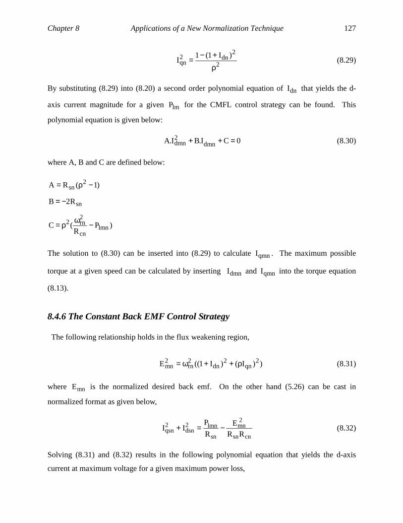
Chapter 8 Applications of a New Normalization Technique 127
2
2dn2
qn)I1(1
Iρ+−= (8.29)
By substituting (8.29) into (8.20) a second order polynomial equation of dnI that yields the d-
axis current magnitude for a given lmP for the CMFL control strategy can be found. This
polynomial equation is given below:
0CI.BI.A dmn2dmn =++ (8.30)
where A, B and C are defined below:
)1(RA 2sn −ρ=
snR2B −=
)PR
(C lmncn
2rn2 −ωρ=
The solution to (8.30) can be inserted into (8.29) to calculate qmnI . The maximum possible
torque at a given speed can be calculated by inserting dmnI and qmnI into the torque equation
(8.13).
8.4.6 The Constant Back EMF Control Strategy
The following relationship holds in the flux weakening region,
))I()I1((E 2qn
2dn
2rn
2mn ρ++ω= (8.31)
where mnE is the normalized desired back emf. On the other hand (5.26) can be cast in
normalized format as given below,
cnsn
2mn
sn
lmn2dsn
2qsn RR
ER
PII −=+ (8.32)
Solving (8.31) and (8.32) results in the following polynomial equation that yields the d-axis
current at maximum voltage for a given maximum power loss,

Chapter 8 Applications of a New Normalization Technique 128
0CI.BI.A dpn2dpn =++ (8.33)
where,
21A ρ−=
2B =
1E
RRE
R
PC
2rn
2mn
cnsn
2mn2
sn
lmn2 +ω
−ρ−ρ=
The negative zero of this polynomial is dmnI . qmnI can be derived by inserting dmnI into (8.32).
The maximum possible torque at a given speed can then be found by inserting dmnI and qmnI
into the torque equation (8.13). The fundamental value of the maximum possible torque under
the SSV control strategy can be found by replacing mnE in the above derivations with the
normalized fundamental component of phase voltage.
8.5 DERIVATION OF MAXIMUM CURRENT REQUIREMENT WITH CPL
In this section the maximum continuous current requirement of a drive operating with constant
power loss is derived as a function of rated current. At rated speed the normalized value of speed
is 1 p.u. The d-axis current is zero by definition of rated torque for PMSM. Therefore, the total
power loss at rated speed and torque can be described as,
)I1(R
1IRP 2
srn2
cn
2srnsnlrn ρ++= (8.34)
where the subscript r denotes that the respective variable is at rated value. It is assumed here that
the maximum possible power loss at any speed is the rated power loss, lrnP . It is seen from Fig.
5.2 that the maximum current requirement happens at zero speed for a motor drive operating
with constant power loss. Core losses are zero at zero speed. Therefore, at zero speed,
2smnsnlrn IRP = (8.35)
where smnI is the maximum possible current. It can be concluded from (8.34) and (8.35) that,
Chapter 8 Applications of a New Normalization Technique 129
)I1(R
1IRIR 2
srn2
cn
2srnsn
2smnsn ρ++= (8.36)
The maximum current can be calculated from (8.36) as:
5.0
cnsn
2srn
cnsn
2
smn )RR1
I)RR
1((I +ρ+= (8.37)
The ratio of maximum current to rated current can be written as given below using (8.37),
5.0
srn
smn )1(I
I α+= (8.38)
where,
cnsn2srncnsn
2
RRI
1
RR+ρ=α (8.39)
The ratio of maximum current to rated current for the prototype PMSM drive described in
Appendix I is 1.35 as calculated from equation (8.38). Therefore, the maximum possible current
for the prototype machine is 35% above rated torque for operation at a load duty cycle of 1 at
zero speed. This maximum current requirement remains valid at very low speeds as well. This
is due to the fact that maximum current vs. speed profile of a machine does not drop off
significantly at very low speeds. This can be seen from Fig. 3.2.
8.6 MAXIMUM POSSIBLE TORQUE AS A FUNCTION OF FLUX LINKAGES
The mutual flux linkages control strategy, described in section 2 of Chapter 6, imposes a
maximum permissible torque emnT on the system. This maximum torque is dependent on the
mutual flux linkages, mnλ , and decreases nonlinearly as the mutual flux linkages decreases. In
this section emnT is computed as a function of mnλ and ρ . The following three characteristics
of the system have been implicitly utilized in the derivations,
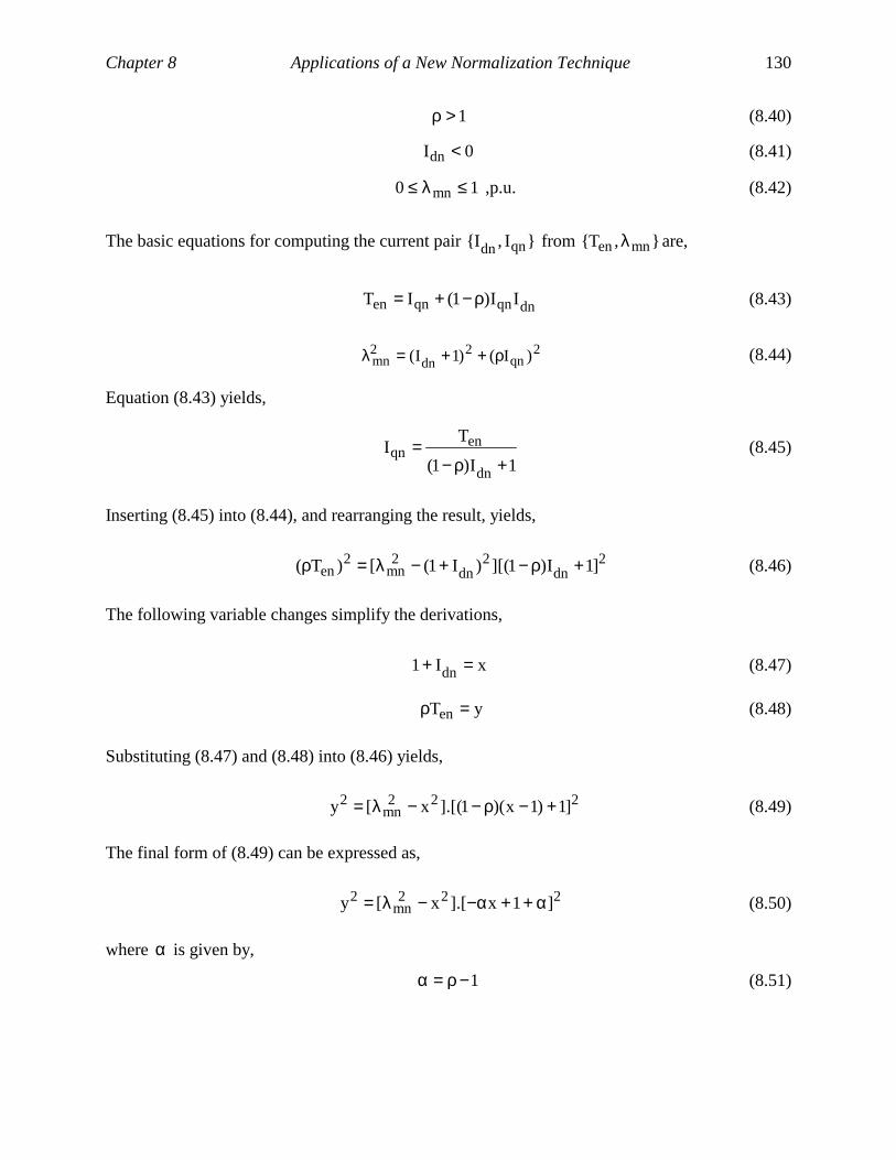
Chapter 8 Applications of a New Normalization Technique 130
1>ρ (8.40)
0Idn < (8.41)
10 mn ≤λ≤ ,p.u. (8.42)
The basic equations for computing the current pair I,I qndn from ,T mnen λ are,
dnqnqnen II)1(IT ρ−+= (8.43)
2qn
2dn
2mn )I()1I( ρ++=λ (8.44)
Equation (8.43) yields,
1I)1(
TI
dn
enqn
+ρ−= (8.45)
Inserting (8.45) into (8.44), and rearranging the result, yields,
2dn
2dn
2mn
2en ]1I)1][()I1([)T( +ρ−+−λ=ρ (8.46)
The following variable changes simplify the derivations,
xI1 dn =+ (8.47)
yTen =ρ (8.48)
Substituting (8.47) and (8.48) into (8.46) yields,
222mn
2 ]1)1x)(1].[(x[y +−ρ−−λ= (8.49)
The final form of (8.49) can be expressed as,
222mn
2 ]1x].[x[y α++α−−λ= (8.50)
where α is given by,
1−ρ=α (8.51)
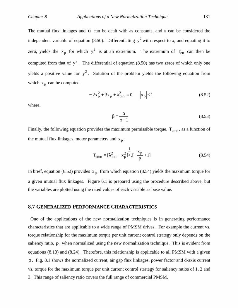
Chapter 8 Applications of a New Normalization Technique 131
The mutual flux linkages and α can be dealt with as constants, and x can be considered the
independent variable of equation (8.50). Differentiating 2y with respect to x, and equating it to
zero, yields the px for which 2y is at an extremum. The extremum of enT can then be
computed from that of 2y . The differential of equation (8.50) has two zeros of which only one
yields a positive value for 2y . Solution of the problem yields the following equation from
which px can be computed.
1x0xx2 p2mnp
2p ≤=λ+β+− (8.52)
where,
1−ρρ=β (8.53)
Finally, the following equation provides the maximum permissible torque, emnT , as a function of
the mutual flux linkages, motor parameters and px .
]1x
.[]x[T p2
12p
2mnemn +
β−−λ= (8.54)
In brief, equation (8.52) provides px , from which equation (8.54) yields the maximum torque for
a given mutual flux linkages. Figure 6.1 is prepared using the procedure described above, but
the variables are plotted using the rated values of each variable as base value.
8.7 GENERALIZED PERFORMANCE CHARACTERISTICS
One of the applications of the new normalization techniques is in generating performance
characteristics that are applicable to a wide range of PMSM drives. For example the current vs.
torque relationship for the maximum torque per unit current control strategy only depends on the
saliency ratio, ρ , when normalized using the new normalization technique. This is evident from
equations (8.13) and (8.24). Therefore, this relationship is applicable to all PMSM with a given
ρ . Fig. 8.1 shows the normalized current, air gap flux linkages, power factor and d-axis current
vs. torque for the maximum torque per unit current control strategy for saliency ratios of 1, 2 and
3. This range of saliency ratio covers the full range of commercial PMSM.
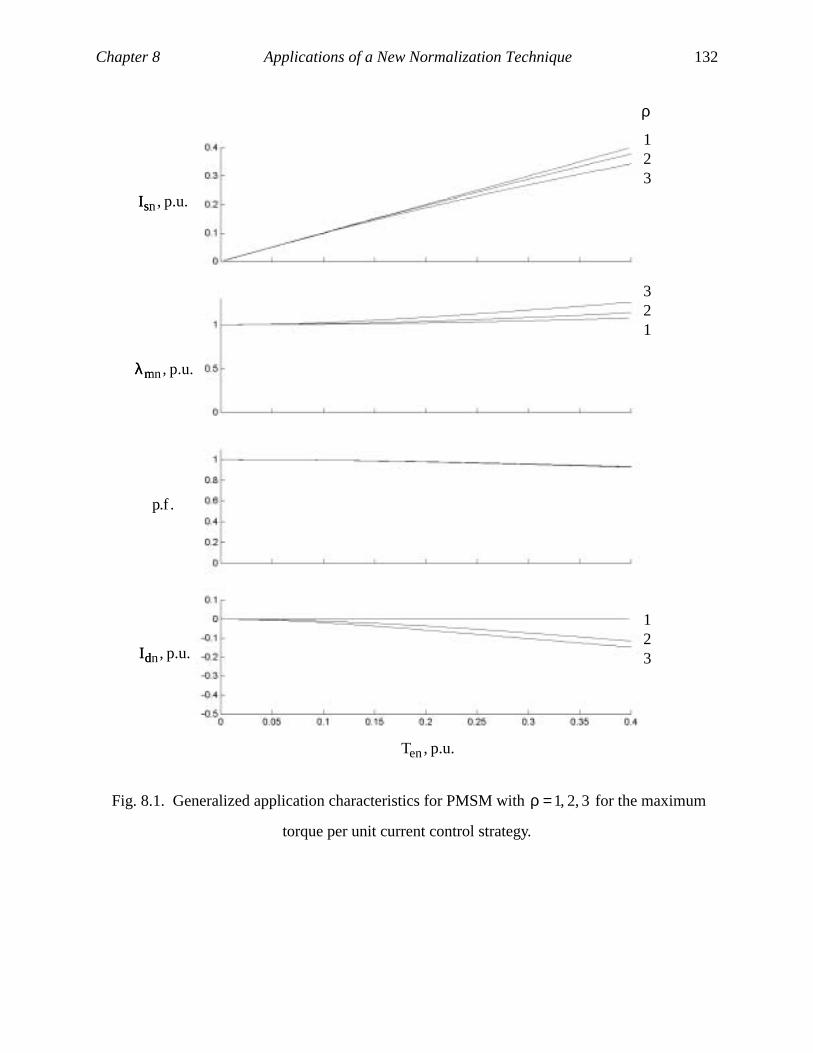
Chapter 8 Applications of a New Normalization Technique 132
Fig. 8.1. Generalized application characteristics for PMSM with 3,2,1=ρ for the maximum
torque per unit current control strategy.
p.u.,Isn
p.u.,mnλ
.f.p
p.u.,Idn
p.u.,Ten
123
123
321
ρ
p.u.,Isn
p.u.,mnλ
.f.p
p.u.,Idn
p.u.,Ten
123
123
321
ρ

Chapter 8 Applications of a New Normalization Technique 133
Note that 1 p.u. of a variable shown in Fig. 8.1 does not correspond to the rated value of the
respective variable. For example 1 p.u. of current and torque as shown in Fig. 8.1 correspond to
17.6 A and 6.5 N.m., respectively, if applied to the prototype motor drive used in this
dissertation. The equivalence of 1 p.u. for each variable can be derived using the base values
described in equations (8.15) to (8.18). The rated current and torque for the prototype motor
drive used in this dissertation are 6.6 A and 2.4 N.m., respectively. Therefore, the rated current
and torque correspond to 0.375 and 0.37 p.u., respectively, in Fig. 8.1.
One of the distinct conclusions that can be made from Fig. 8.1 is that the power factor for
PMSM with the maximum torque per unit current control strategy is not affected very much by
the saliency ratio. The power factor shown in Fig. 8.1 is calculated assuming that the difference
between the back emf and the phase voltage is negligible. It is also seen that the current required
at any given torque decreases as the saliency ratio increases, and the required magnitude of d-
axis current increases at the same time. Fig. 8.2 shows the same performance characteristics as
shown in Fig. 8.1 but with the zero d-axis current control strategy. It is seen here that the power
factor drops significantly as the saliency ratio increases for the zero d-axis current control
strategy. The current vs. torque characteristic is not affected by saliency ratio in this case.
Chapter 8 Applications of a New Normalization Technique 134
Fig. 8.2. Generalized application characteristics for PMSM with 3,2,1=ρ for the
zero d-axis current control strategy.
p.u.,Isn
p.u.,mnλ
.f.p
p.u.,Idn
p.u.,Ten
123
321
ρ
p.u.,Isn
p.u.,mnλ
.f.p
p.u.,Idn
p.u.,Ten
123
321
ρ

Chapter 8 Applications of a New Normalization Technique 135
8.8 CONCLUSIONS
A new normalization technique is introduced in this chapter. The magnet flux linkages and d-
axis inductance are chosen as base values so that these two parameters are eliminated from all
equations. This normalization technique simplifies the analysis and simulation of a PMSM
motor drive. Comparison to other normalization techniques shows the superiority of the new
technique. Analytical terms for the maximum torque vs. speed envelopes for the ME, MTPC,
ZDAC, UPF, CMFL and CBE control strategies are derived in this chapter using the new
normalization technique. The maximum continuous current requirement of a motor drive
operating with constant power loss is derived as a function of the motor’s rated current. The
maximum possible torque as a function of desired mutual flux linkages is also derived. The new
normalization technique can be used to generate generalized application characteristics for
PMSM drives. This is demonstrated for the maximum torque per unit current and zero d-axis
current control strategies. It is clear through all these derivations that the new normalization
technique simplifies and facilitates the analysis and simulation of high performance PMSM
drives.
The contributions of this chapter are summarized below:
• Introduction of a new normalization technique
• Derivation of the maximum torque vs. speed envelopes for the ME, MTPC, ZDAC, CMFL,
UPF, CBE control strategies operating with constant power loss
• Derivation of the maximum current requirement of a PMSM drive with constant power loss
• Derivation of the maximum possible torque for a given mutual flux linkages
• Introduction of generalized application characteristics for PMSM drives
136
CHAPTER 9
Conclusions and Recommendations for Future Work
9.1 CONCLUSIONS
The main achievements of this dissertation are summarized below:
• Analysis of the operational boundary of variable speed PMSM drives
• Introduction of a control strategy that automatically limits the operational boundary of a
motor drive
• Analysis and comparison of different strategies for high performance control of PMSM
• Introduction of implementation techniques for concurrent mutual flux linkages and torque
control in the flux weakening range of operation for PMSM
• Introduction of implementation techniques for concurrent mutual flux linkages and torque
control in the flux weakening range of operation for PMSM in the presence of parameter
variations
• Introduction of a normalization technique that simplifies the analysis and simulation of
PMSM drive performance.
The traditional method of defining and implementing the operational boundary of a motor drive
is to limit torque and power to rated values. It is shown here that the traditional method results in
under-utilization of the machine and puts the system at risk of excessive power losses. The
constant power loss concept is introduced and analyzed here as the correct basis for defining and
studying the operational boundary of any motor drive. The implementation strategy for the
proposed scheme is developed. All major control strategies for linear torque control for PMSM
are analyzed and compared based on the constant power loss concept. The ME, MTPC, ZDAC,
UPF and CMFL control strategies are the main possible choices for the lower than base speed
operating range. The CBE and SSV control strategies are the main possible choices for the
higher than base speed operating range. Each set of control strategies results in a unique
Chapter 9 Conclusions and Recommendations for Future Work 137
operational boundary and performance. Therefore, the comparison provided in this dissertation
allows for choosing the optimal control strategy for a particular application.
The implementation of the constant power loss controller is achieved using a feedback loop
around a linear torque controller for PMSM. The area of implementation strategies for linear
torque control in the lower than base speed operating range has been adequately covered in the
literature. The area of torque control in the flux weakening range is revisited here. Practical
implementation strategies for the concurrent flux weakening and torque control for PMSM are
introduced in this dissertation. Also, implementation strategies for the concurrent flux
weakening and torque control in the presence of parameter variation are presented.
A new normalization technique is introduced that simplifies the analysis of PMSM motor
drives. The new normalization technique is shown to simplify the performance analysis for
PMSM drives. All derivations and simulations presented in this dissertation are performed using
the new normalization technique.
The contributions of this dissertation are summarized below:
• A constant power loss (CPL) based control strategy to obtain the maximum torque vs. speed
envelope
• An implementation scheme for the proposed constant power loss controller
• Calculation of the appropriate power loss command and maximum torque for the CPL
controller applied to applications with cyclic loads
• Comparison of maximum possible torque as a function of maximum possible power loss for
different applications with cyclic loads
• Performance analysis of different control strategies for PMSM along the constant power loss
operational envelope
• Comparison of control strategies along the constant power loss operational envelope
• Comparison of control strategies inside the constant power loss operational envelope
• Derivation of maximum speed, current and torque as a function of maximum power loss and
machine parameters

Chapter 9 Conclusions and Recommendations for Future Work 138
• Introduction of two practical implementation schemes, based on lookup tables or equations,
for the concurrent mutual flux linkages weakening and torque control for PMSM
• Analysis of the maximum possible torque as a function of the desired mutual flux linkages
• Procedure for computing the current vector compensation offset using lookup tables or neural
networks for high performance control of PMSM in the presence of parameter variations
• Introduction of a new normalization technique that simplifies the analysis and simulation
PMSM drive performance
• Derivation of the maximum torque vs. speed envelopes for the ME, MTPC, ZDAC, CMFL,
UPF, CBE control strategies operating with constant power loss
• Introduction of generalized application characteristics for PMSM drives using the new
normalization technique
• Experimental verification of key results
9.2 RECOMMENDATIONS FOR FUTURE WORK
The concepts presented in this dissertation are all demonstrated using PMSM drives. However,
all of these concepts equally apply to all motor drives. The next major step is to apply the
constant power loss controller to high performance PM brushless dc, induction, switched
reluctance and synchronous reluctance drives. The performance of different control strategies
for these motor drives need to be analyzed and compared based on the constant power loss
concept. Also, the implementation schemes presented here for concurrent flux weakening and
torque control for PMSM should be applied to the other types of drives mentioned above.

139
APPENDIX I
Prototype PMSM Drive
A high performance prototype PMSM drive is utilized in experimentally verifying the key
results of this dissertation. The prototype is assembled on bread-board, and is developed entirely
in hardware with no software programmable components. The motor drive block diagram is
shown in Fig. 3.3. A 16 bit resolver to digital converter is used to generate rotor position
feedback. Only 8 bits of this feedback are utilized in practice. The speed feedback is derived by
filtering the least significant bit of the resolver to digital output. The torque command is
digitized using 8 bits, and the speed feedback is digitized using 5 bits. The digitized torque and
speed are the inputs to two 8 kb EEPROMs. Each of these EEPROMs outputs an 8 bit command
for current magnitude and angle with respect to rotor, respectively. A desired control strategy
must be written into these EEPROMs. A vector rotator uses the position feedback and the digital
values for current magnitude and angle commands to generate phase a, b and c current
commands. Phase a, b and c current commands are then enforced on the machine using three
independent 10 kHz PWM current controllers. Current feedback is provided by two LEM
modules. The power stage uses six IGBTs (600V, 50A), and is capable of handling 10 Amperes
at 250 Volts.
The interior PMSM parameters are:
qL = 12.5 mH, dL = 5.7 mH, afλ = 123 mWeber-turns, P= 4, sR = 1.2 Ω , cR = 416 Ohms,
dcV = 118 Volts (Bus voltage).
The rated values of the system are given below:
speed = 3500 RPM, current = 6.6 A, torque = 2.4 N.m., power = 890 W, power loss = 121 W,
core losses at rated operating point = 43 W, copper losses at rated operating point = 78 W.
Combined motor and load inertia=0.0019 Kg. 2m , friction coefficient=2.7e-4 N.m./Rad/s.

140
APPENDIX II
Measurement of PMSM Parameters
The parameters of the PMSM described in Appendix I are measured as described below:
sR : The phase resistance is measured by dividing the line to line resistance by two. The line to
line resistance is measured by applying a known current and measuring the voltage drop across
the line to line terminal, or using an Ohm meter.
afλλλλ : The machine is back driven at a known speed. The peak of the line to line voltage divided
by square root of 3 is the phase back emf in this case. Rotor flux linkages can then be calculated
using the following equation,
ω=λ E
af (1)
cR : First the PMSM, with leads open, is back driven at a relatively low speed using a dc motor.
Any speed in the range of 100 to 300 RPM is fine. A relatively low speed is chosen so that only
a negligible magnitude of core losses is present. Then the power input to the dc motor is
measured. This input power is almost entirely indicative of the sum of copper and brush losses
on the dc motor and net friction losses. The friction losses can then be calculated by subtracting
dc motor copper and brush losses from the net input power to the dc motor. Note that the dc
motor current and phase resistance are known. Brush losses are negligible in this case. The
friction torque of the combined dc and PMSM setup can be calculated by dividing the estimated
friction losses by speed. Then the PMSM is back driven at 3500 RPM (rated speed) using the
same dc motor. The power input to the dc motor at 3500 RPM is the sum of copper losses of the
dc motor, friction losses, core losses of PMSM and windage losses. The friction losses can be
estimated by multiplying speed with the friction torque calculated before. The windage losses of
the dc motor is assumed to be negligible. The windage losses of the PMSM is estimated using

Appendix II Measurements of PMSM Parameters 141
the viscous damping coefficient (N.m./kRPM) given in manufacturer’s data sheets. The input
power to the dc motor net of dc motor copper losses, friction losses and windage losses of
PMSM is core losses of the PMSM. The core loss resistance, as defined in Fig. 3.1, can then be
calculated using the following equation,
l
22af
c P
5.1R
ωλ= (2)
where lP is defined here as being the net core loss calculated earlier.
qL and dL : q and d-axis inductances are measured by shorting phases b and c of a PMSM, and
measuring inductance across phases a and b while the rotor is locked. With phases b and c
shorted, the d-axis current in rotor reference fame is eliminated assuming that the q-axis of the
rotor is aligned with phase a. Therefore, the d-axis portion of the PMSM electrical model does
not contain any useful information in this case as back emf is also zero. The electrical model of
the machine can then be described as given below,
aqrass iLiRv ω+= (3)
Note that the q-axis and phase a currents are the same in this case. The q-axis of the rotor can be
aligned with phase a by finding the rotor position that yields minimum peak to peak current in
response to a fixed sinusoidal voltage input applied to phases a and b. Once this minimum peak
to peak current in known qL can be identified using the following equation,
2s
2r
2q
2
pp
ppRL)
I
V( +ω= (4)
where ppV and ppI are the peak to peak values of the input voltage and phase a current,
respectively, and rω is the frequency of input voltage times π2 . Alternatively, qL , can be
estimated by measuring the electrical time constant of the system using the following equation,
s
qll R
L=τ (5)
Appendix II Measurements of PMSM Parameters 142
Note that the rotor must be locked while making all measurements described above. The same
procedure as described above yields dL if the rotor position is such that ppI is maximized in
response to a fixed sinusoidal voltage input.
The lowest possible frequency for the input voltage yields the most accurate estimation of
inductance since the impact of core losses are minimum at lower frequencies. A frequency of 60
Hz is chosen in the case of this dissertation. Therefore, the inductance measurements are subject
to some degree of error due to core losses. Core losses cause discrepancies between the
measured and actual parameters while using the electrical time constant technique for the
measurement of inductance as well. This is especially true when measuring dL where the rate
of rise of current in response to a step input voltage is maximum.

143
References
[1] Encyclopedia Brittanica, “Electricity and Magnetism,” Macropedia, Vol. 18, pp. 193-194,
1995.
[2] T.C. Martin and J. Wetzler, “The Electric Motor and its Applications”, book, W.J. Johnston,
Publisher, 1887.
[3] Nikolai Tesla, “A New System of Alternate Current Motors and Transformers,” AIEE
Transactions, 1888.
[4] A. Blondel, “Synchronous motor and converter, Part III,” book, McGraw-Hill, New York,
1913.
[5] R.H. Park, “Two reaction theory of synchronous machines- Part I,” AIEE Transactions, Vol.
48, No. 2, 1929, pp.716-730.
[6] F. Blaschke, “The principle of field orientation as applied to the new Transvektor closed-loop
control system for rotating field machines,” Siemens Review XXXIX, 1972, pp. 217-220.
[7] R. Krishnan, “Electronic Motor Drives Modeling, Analysis and Control,” book, Prentice
Hall, February 2001.
[8] R. Krishnan, “Control and Operation of PM Synchronous Motor Drives in the Field-
Weakening Region”, Conference Record, IEEE IECON, 1993, pp. 745-750.
[9] B. Chalmers, “Variable-Frequency Synchronous Motor Drives for Electric Vehicles,” IEEE
Transactions on Industry Applications, Vol. 32, No. 4, July/August 1996, pp. 896-903.
[10] G. Slemon, “High-Efficiency Drives Using Permanent-Magnet Motors,” IECON
Proceedings, 1993, pp. 725-730.
[11] M. Rahman, “High Efficiency Permanent Magnet Synchronous Motors,” IEEE IAS
Meeting, 1979, pp. 561-564.
References 144
[12] P. Pillay and R. Krishnan, “Application Characteristics of PM Synchronous and BDCM
Motor Servo Drives,” Conf. Record, IEEE IAS Annual Meeting, Atlanta, Oct. 1987, pp. 380-390.
[13] G. Slemon and Xiau Liu, “Core Losses in Permanent Magnet Motors,” IEEE Transactions
on Magnetics, Vol. 26, No. 5, September 1990, pp. 1653-1656.
[14] T.J.E. Miller, “Back EMF waveform and Core Losses in Brushless DC Motors,” IEE
Proceedings- Electrical Power Applications, Vol. 141, No. 3, May 1994, pp. 144-154.
[15] G. Bertotti, A. Boglietti, et al, “An Improved Estimation of Iron Losses in Rotating
Electrical Machines,” IEEE Transactions on Magnetics , Vol. 27, No. 6, November 1991, pp.
5007-5009.
[16] S. Morimoto, et al, “Rotor design optimization of a multi-layer interior permanent-magnet
synchronous motor,” IEE Proceedings-Electrical Power Applications, Vol. 145, No. 2, March
1998, pp. 119-124.
[17] R.S. Colby and D.W. Novotny, “Efficient Operation of PM Synchronous Motors,” IEEE
Transactions on Industry Applications, vol. IA-23Nov./Dec. 1987, pp. 1048-1054.
[18] S. Morimoto, et al, “Loss Minimization Control of Permanent Magnet Synchronous Motor
Drives,” Transactions on Industry Applications, Vol. 41., NO. 5, October 1994, pp. 511-517.
[19] R. Schiferl and T.A. Lipo, “Core Losses in Buried Magnet Permanent Magnet Synchronous
Motors,” IEEE Transactions On Energy Conversion, Vol. 4, No. 2, June 1989, pp. 279-284.
[20] T. Lipo, et al, “Vector Control of a Synchronous Reluctance Motor Including Saturation and
Iron Loss,” IEEE Transactions on Industry Applications, Vol. 27, No. 5, September/October
1991, pp. 978-985.
[21] J. Flecher, et al, “Efficiency Aspects of Vector Control Applied to Synchronous Reluctance
Motors,” Conference Proceedings, IEEE IAS meeting, 1995, pp. 294-300.
[22] F. Fernandez-Bernal, et al, “Efficient Control of Reluctance Synchronous Machines,” IEEE
IECON, 1998, pp. 923-928.
References 145
[23] A.E. Fitzgerald, C. Kingsley, Jr. and S.D. Umans, “Electric Machinery,” book, McGraw-
Hill International Book Company, fourth edition, 1983.
[24] N. Bianchi and S. Bolognani, “Parameters and Volt-Ampere Ratings of a Synchronous
Motor Drive for Flux Weakening Applications,” IEEE Transactions on Power Electronics, Vol.
12, No. 5, September 1997, pp. 895-903.
[25] S. Morimoto and Y. Takeda, “Generalized Analysis of Operating Limits on PM Motor and
Suitable Machine Parameters for Constant-Power Operation,” Electrical Engineering in Japan,
Vol. 123, No. 3, 1988, pp. 55-63.
[26] S. Morimoto, et al, “Optimum Machine Parameters and Design of Inverter-Driven
Synchronous Motors for Wide Constant Power Operation,” IEEE IAS annual meeting, 1994, pp.
177-182.
[27] S. Morimoto, et al, “Wide-Speed Operation of Interior Permanent Magnet Synchronous
Motors with High-Performance Current Regulators”, IEEE Transactions on Industrial
Applications, Vol. 30, July/August 1994, pp. 920-925.
[28] T. Sebastian and G.R. Slemon, “Operating Limits of Inverter-driven Permanent Magnet
Motor Drives,” IEEE Transactions on Industry Applications, Vol. IA-23, No. 2, March/April
1987, pp. 327-333.
[29] S. Morimoto, Y. Takeda and T. Hirasa, “Current Phase Control Methods for PMSM,” IEEE
Transactions on Power Electronics, Vol. 5, No. 2, April 1990, pp. 133-138.
[30] P. Pillay and R. Krishnan, “Modeling, analysis and simulation of high performance, vector
controlled, permanent magnet synchronous motors,” conference record, IEEE Industry
Applications Society Meeting, 1987, pp. 253-261.
[31] T.M. Jahns, et al, “Interior Permanent -Magnet Synchronous Motors for Adjustable-Speed
Drives,” IEEE Transactions on Industry Applications, Vol. IA-22, NO. 4, July/August 1986, pp.
738-747.

References 146
[32] S. Morimoto, K. Hatanaka and Y. Tong, Y. Takeda and T. Hirasa, “Servo Drive System and
Control Characteristics of Salient Pole Permanent Magnet Synchronous Motor,” IEEE
Transactions on Industry Applications, Vol. 29, No. 2, Mar./Apr. 1993, pp. 338-343.
[33] T.M. Jahns, “Flux-Weakening Regime Operation of an Interior Permanent-Magnet
Synchronous Motor Drive,” IEEE Transactions on Industry Applications, Vol. IA-23, No. 4,
July/August 1987, pp. 681-689.
[34] Magureanu, R., "A state variable analysis of inverter-fed a.c. machines", Revue Roumaine
des Sciences Techniques, Serie Electrotechnique et Energetique, vol.18, no.4, pp. 663-78, 1973.
[35] A. Fratta, A. Vagati, F. Villata, “Extending the Voltage Saturated Performance of a DC
Brushless Drive,” Europian Power Electronics Conference FIRENZE, 1991.
[36] G. Shaefer, “Field Weakening of Brushless Permanent Magnet Servomotor with
Rectangular Current,” Europian Power Electronics Conference FIRENZE, 1991, pp. 3-429,3-
434.
[37] B. Sneyers, et al, “Field Weakening in Buried Permanent Magnet AC Motor Drives,” IEEE
Transactions on Industry Applications, Vol. IA-21, No. 2, March/April 1985, pp. 398-407.
[38] J. Kim and S. Sul, “Speed Control of Interior Permanent Magnet Synchronous Motor Drive
for the Flux Weakening Operation,” IEEE Transactions on Industry Applications, Vol. 33, No. 1,
Jan./Feb. 1997, pp. 43-48.
[39] B.K. Bose, “A high-performance Inverter-Fed Drive System of an Interior PMSM”, IEEE
Transactions on Industry Applications, Vol. 24, No. 6, Nov./Dec. 1988.
[40] S. Morimoto, et al, “Effects and Compensation of Magnetic Saturation in PMSM drives”,
Conference record, IEEE Transactions on Industry Applications, Vol. 30, n6, November-
December 1994, pp. 1632-1637.
[41] T. Sebastian, “Temperature Effects on Torque Production and Efficiency of PM Motors
Using NdFeB Magnets,” IEEE Transactions on Industry Applications, Vol. 31, No. 2, Mar./Apr.
1995, pp. 353-357.

References 147
[42] R. Krishnan and P. Vijayraghavan, “Parameter Compensation of Permanent Magnet
Synchronous Machines Through Airgap Power Feedback,” IEEE Industrial Electronics
Conference, Nov. 1995.
[43] R. Krishnan and P. Vijayraghavan, “Fast Estimation and Compensation of Rotor Flux
Linkage in Permanent Magnet Synchronous Machines,” Proceedings of the International
Symposium on Industrial Electronics, Vol. 2, 1999, pp. 661-666.
[44] R. Monajemy and R. Krishnan, “Concurrent mutual flux and torque control for the
permanent magnet synchronous motor,” Conference record, IEEE Industry Applications Society
Annual Meeting, Oct. 1995, pp. 238-245.
[45] R. Monajemy and R. Krishnan, “Control and dynamics of constant power loss based
operation of permanent magnet synchronous motor,” IEEE Industrial Electronics Conference,
Nov. 29-Dec. 3, 1999, pp. 1452-1457.
[46] R. Monajemy and R. Krishnan, “Performance comparison of six-step voltage and constant
back emf control strategies for PMSM,” Conference record, IEEE Industry Applications Society
Annual Meeting, Oct. 1999, pp. 165-172.
[47] R. Krishnan, R. Monajemy and N. Tripathi, “Neural Control of High Performance Drives:
An Application to the PM Synchronous Motor Drive”, Invited Paper, Conference records, IEEE
Industrial Electronics Conference (IECON), November, 1995, pp. 38-43.
[48] F. Thornton, “Electric Home Appliances- 100 years,” Electrical Engineering, AIEE, vol.
71, 1952, pp. 1087-90.
[49] R. Krishnan, S. Lee and R. Monajemy, “Modeling, dynamic analysis and simulation of a c-
dump brushless dc motor”, Conference Records, APEC, 1996.
[50] G.R. Slemon, “Achieving a constant power speed range for PM drives,” IEEE Transactions
on Industry Applications, Vol. 31, No. 2, March/April 1995, pp. 368-372.
[51] P. Pillay and R. Krishnan, “Control characteristics and speed controller design for a high
performance permanent magnet synchronous motor drive,” conference record, Power
Electronics Specialist Conference, 1987, pp. 598-606.

References 148
[52] P. Enjeti, J.F. Lindsay and M.H. Rashid, “ Parameter estimation and dynamic performance
of permanent magnet synchronous motor,” conference record, IAS meeting, 1985, pp. 627-633.
[53] Charlton, W., "Matrix method for the steady-state analysis of inverter-fed induction
motors", Proceedings of the IEE, vol.120, no.3, pp. 363-364, March 1973.
[54] Lipo, T.A. and Turnbull, F.G., "Analysis and comparison of two types of square wave
inverter drives", Proceedings of the 1972 Seventh Annual Meeting of the IEEE Industry
Applications Society, pp. 127-36, Oct. 1972.
[55] Ramamoorty, M., "Steady state analysis of inverter driven induction motors using harmonic
equivalent circuits", 8th Annual Meeting of the IEEE Industry Applications Society, pp. 437-40,
Oct. 1973.
[56] I. Boldea and S.A. Nasar, “Unified Treatment of Core Losses and Saturation in Orthogonal-
axis Model of Electric Machines,” IEE Proceedings, Vol. 134m Pt. B, No. 6, November 1987,
pp. 355-363.
[57] N. Stranges and R.D.Findlay, “Importance of Rotational Data for Accurate Prediction of
Rotating Machine Core Losses,” IEEE IAS Annual Meeting, 1994, pp. 123-127.
[58] A.G. Jack, B. C. Mecrow and J.A. Haylock, “A Comparative Study of Permanent Magnet
and Switched Reluctance Motors for High-Performance Fault-Tolerant Applications,” IEEE
Transactions Industry Applications, Vol. 32, No. 4, July/Aug. 1996, pp. 889-895.
[59] A. Boglietti, et al, “About the Design of Very High Frequency Induction Motors for Spindle
Applications,” Electric Machines and Power Systems, Vol. 25, n4, May 1997, pp. 387-409.
[60] A. Vagati, et al, “High-Performance Control of Synchronous Reluctance Motors,” IEEE
Transactions on Industry Applications, Vol. 33, n4, July-August 1997, pp. 983-991.
[61] T. Matsao, A. El-Antably and T. Lip, “A New Control Strategy for Optimum-Efficiency
Operation of a Synchronous Reluctance Motor,” IEEE Transactions on Industry Applications,
Vol. 33, No. 5, September/October 1997, pp. 1146-1153.

References 149
[62] V. B. Honsinger, “The Fields and Parameters of Interior Type AC Permanent Magnet
Machines,” IEEE Transactions on Power Apparatus and Systems, Vol. PAS-101, No. 4, April
1982, pp. 867-875.
[63]K. Miyashita, et al, “Development of High Speed 2-Pole Permanent Magnet Synchronous
Motor,” IEEE PES Winter Meeting, 1979, pp. 2176-2182.
[64] S. Williamson and R.G. Cann, “A Comparison of PWM Switching Strategies on the Basis
of Drive System Efficiency,” IEEE Transactions on Industry Applications, Vol. IA-20, No. 6,
November/December 1984, pp. 1460-1472.
[65] R. Krishnan and P. Pillay, “Parameter Sensitivity in Vector Controlled AC Motor Drives,”
IEEE IECON, 1987, pp. 212-218.
[66] H.G. Hamed, “Current Requirements of the Switching Elements of a 3-Phase VSI Feeding a
3-Phase Induction Motor,” Modeling, Measurement & Control, A, AMSE Press, Vol. 57, No. 2,
1994, pp. 29-42.

150
Vita
Ramin Monajemy received his B.Sc. degree in electrical engineering in 1988 from Sharif
University of Technology, Tehran, Iran. He received his M.Sc. degree in electrical engineering
in 1993 from George Mason University, Fairfax, VA, where he studied the field of model-based
fault detection and isolation, and published two papers on that subject. His current research
areas involve the high performance control of motor drives.