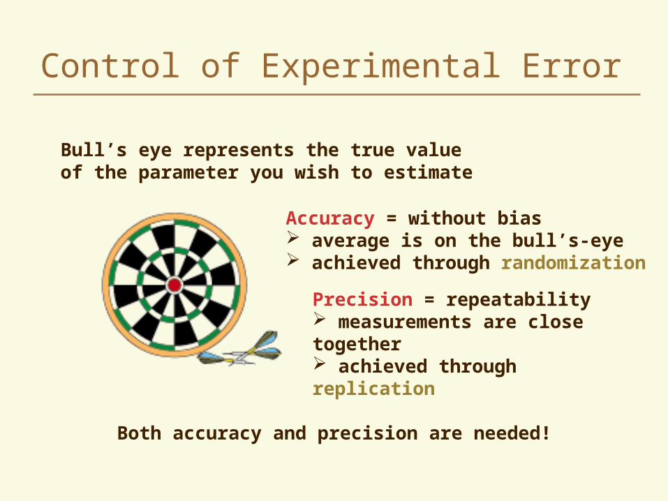
Control of Experimental Error

Accuracy = without bias average is on the bull’s-eye achieved through randomization

Precision = repeatability measurements are close together achieved through replication

Bull’s eye represents the true valueof the parameter you wish to estimate

Both accuracy and precision are needed!

To eliminate bias

To ensure independence among observations

Required for valid significance tests and interval estimates

Old New Old New Old New Old New

In each pair of plots, although replicated, the new variety is consistently assigned to the plot with the higher fertility level.

Low High

Randomization

Replication The repetition of a treatment in an experiment

A A

A

B

B

B

CC

C

D

D

D

Replication

Each treatment is applied independently to two or more experimental units

Variation among plots treated alike can be measured

Increases precision - as n increases, error decreases

Sample variance

Number of replications

Standard error of a mean

Broadens the base for making inferences

Smaller differences can be detected

Effect of number of replicates

Effect of replication on variance

0.00.51.01.52.02.53.03.54.04.55.05.56.06.57.07.58.0

0 5 10 15 20 25 30 35 40 45 50

number of replicates

Var

ian

ce o

f th

e m

ean

What determines the number of replications?

Pattern and magnitude of variability in the soils

Number of treatments

Size of the difference to be detected

Required significance level

Amount of resources that can be devoted to the experiment

Limitations in cost, labor, time, and so on

Strategies to Control Experimental Error

Select appropriate experimental units

Increase the size of the experiment to gain more degrees of freedom– more replicates or more treatments– caution – error variance will increase as more heterogeneous

material is used - may be self-defeating

Select appropriate treatments– factorial combinations result in hidden replications and therefore

will increase n

Blocking

Refine the experimental technique

Measure a concomitant variable– covariance analysis can sometimes reduce error variance

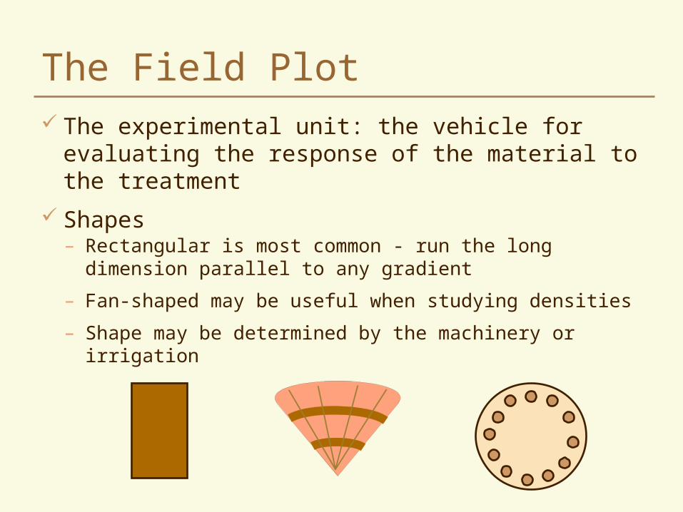
The Field Plot The experimental unit: the vehicle for evaluating

the response of the material to the treatment

Shapes– Rectangular is most common - run the long dimension parallel to

any gradient

– Fan-shaped may be useful when studying densities

– Shape may be determined by the machinery or irrigation

Plot Shape and Orientation

Long narrow plots are preferred– usually more economical for field operations– all plots are exposed to the same conditions

If there is a gradient - the longest plot dimension should be in the direction of the greatest variability

Border Effects

Plants along the edges of plots often perform differently than those in the center of the plot

Border rows on the edge of a field or end of a plot have an advantage – less competition for resources

Plants on the perimeter of the plot can be influenced by plant height or competition from adjacent plots

Machinery can drag the effects of one treatment into the next plot

Fertilizer or irrigation can move from one plot to the next

Impact of border effect is greater with very small plots

Effects of competition In general, experimental materials should be evaluated

under conditions that represent the target production environment

Minimizing Border Effects Leave alleys between plots to minimize drag

Remove plot edges and measure yield only on center portion

Plant border plots surrounding the experiment

Experimental Design An Experimental Design is a plan for the assignment

of the treatments to the plots in the experiment

Designs differ primarily in the way the plots are grouped before the treatments are applied– How much restriction is imposed on the random

assignment of treatments to the plots

A B

C

D A

A

B

B

C

C

D

D

CDA B

A

A

B

B

C

C

D

D

Why do I need a design? To provide an estimate of experimental error

To increase precision (blocking)

To provide information needed to perform tests of significance and construct interval estimates

To facilitate the application of treatments - particularly cultural operations

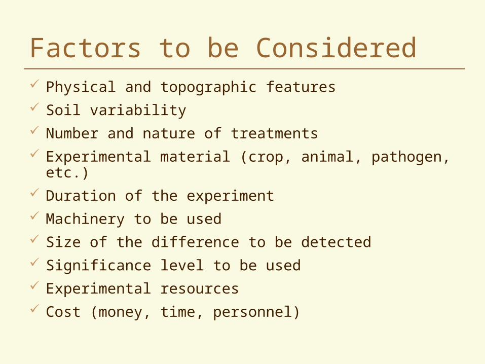
Factors to be Considered Physical and topographic features

Soil variability

Number and nature of treatments

Experimental material (crop, animal, pathogen, etc.)

Duration of the experiment

Machinery to be used

Size of the difference to be detected

Significance level to be used

Experimental resources

Cost (money, time, personnel)

Cardinal Rule:

Choose the simplest experimental design that will give the required precision within the limits of the available resources

Completely Randomized Design (CRD)

Simplest and least restrictive

Every plot is equally likely to be assigned to any treatment

A A

A

B

B

B

CC

C

D

D

D

Advantages of a CRD Flexibility

– Any number of treatments and any number of replications

– Don’t have to have the same number of replications per treatment (but more efficient if you do)

Simple statistical analysis– Even if you have unequal replication

Missing plots do not complicate the analysis

Maximum error degrees of freedom

Disadvantage of CRD Low precision if the plots are not uniform

A B

C

D A

A

B

B

C

C

D

D

Uses for the CRD If the experimental site is relatively uniform

If a large fraction of the plots may not respond or may be lost

If the number of plots is limited

Design Construction No restriction on the assignment of treatments to the

plots

Each treatment is equally likely to be assigned to any plot

Should use some sort of mechanical procedure to prevent personal bias

Assignment of random numbers may be by:– lot (draw a number )– computer assignment– using a random number table

Random Assignment by Lot We have an experiment to test three varieties:

the top line from Oregon, Washington, and Idaho to find which grows best in our area ----- t=3, r=4

1 2 3 4

5 6 7 8

9 10 11 12A

A

A

A

12156

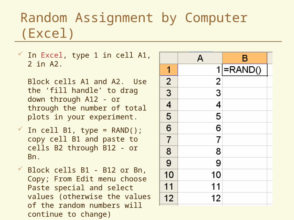
Random Assignment by Computer (Excel)

In Excel, type 1 in cell A1, 2 in A2.

Block cells A1 and A2. Use the ‘fill handle’ to drag down through A12 - or through the number of total plots in your experiment.

In cell B1, type = RAND(); copy cell B1 and paste to cells B2 through B12 - or Bn.

Block cells B1 - B12 or Bn, Copy; From Edit menu choose Paste special and select values (otherwise the values of the random numbers will continue to change)

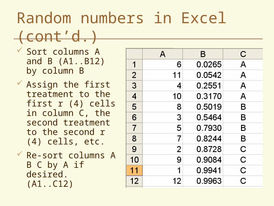
Random numbers in Excel (cont’d.) Sort columns A and B

(A1..B12) by column B

Assign the first treatment to the first r (4) cells in column C, the second treatment to the second r (4) cells, etc.

Re-sort columns A B C by A if desired. (A1..C12)

Rounding and Reporting NumbersTo reduce measurement error:

Standardize the way that you collect data and try to be as consistent as possible

Actual measurements are better than subjective readings

Minimize the necessity to recopy original data

Avoid “rekeying” data for electronic data processing

– Most software has ways of “importing” data files so that you don’t have to manually enter the data again

When collecting data - examine out-of-line figures immediately and recheck

Significant Digits Round means to the decimal place corresponding to

1/10th of the standard error (ASA recommendation)

Take measurements to the same, or greater level of precision

Maintain precision in calculations

If the standard error of a mean is 6.96 grams, then

6.96/10 = 0.696 round means to the nearest 1/10th gram

for example, 74.263 74.3

But if the standard error of a mean is 25.6 grams, then

25.6/10 = 2.56 round means to the closest gram

for example, 74.263 74

In doing an ANOVA, it is best to carry the full number of figures obtained from the uncorrected sum of squares

Do not round closer than this until reporting final results

If, for example, the original data contain one decimal, the sum of squares will contain two places

2.2 * 2.2 = 4.84

Rounding in ANOVA