control of electric vehicles using a model predictive

CONTROL OF ELECTRIC VEHICLES USING A MODEL PREDICTIVE CONTROLLER WITH CLOSED FORM SOLUTION

Milad Jalaliyazdi University of Waterloo

Waterloo, Ontario, Canada

Amir Khajepour University of Waterloo


Shih-Ken Chen R&D General Motors

Warren, MI, USA

ABSTRACT In this paper, the problem of vehicle stability control using

model predictive technique is addressed. The vehicle under

consideration is an electric vehicle with an electric motor

driving each wheel independently. For the purpose of stability

control, it is required that the vehicle tracks a desired yaw rate

at all times therefore, extending the linear range of the vehicle

dynamics. The desired yaw rate is defined based on vehicle

speed, steering wheel angle and road surface friction.

The vehicle stability control system considered in this paper

consists of a high-level controller that compares the current

states of the vehicle with its desired states to determine the

required forces and moments at the center of mass, and a low-

level controller to track those C.G. forces and moments by

adjusting the motor torques on each wheel. It will be shown

that a non-predictive low-level controller can have a closed

form solution. In order to avoid saturation of the tires, the low-

level controller has a penalty function that increases

exponentially when the tire forces are close to the limits of

saturation to reduce tire forces to keep them within the tires

force capacity.

In this paper, a model predictive controller is designed as the

low-level controller to predict the tire forces and the yaw

moment at the C.G. to minimize the tracking error of desired

C.G. forces and moments. To keep the tire forces within the

tires capacity limit, a penalty function is used at each sample

time to penalize control actions that result in excessive tire

forces. This adds a level of anticipation to the low-level

controller to detect in advance when tires are about to saturate

and to choose control actions to prevent that from happening.

Since tire capacity limit is treated with an analytical penalty

function, it is still possible to find a closed form solution for the

model predictive low-level controller. The proposed controller

is tested with simulations and the results are compared with a

similar non-predictive controller.

Alireza Kasaeizadeh University of Waterloo


Bakhtiar Litkouhi R&D General Motors

Warren, MI, USA

Proceedings of the ASME 2014 International Mechanical Engineering Congress and Exposition IMECE2014

November 14-20, 2014, Montreal, Quebec, Canada

IMECE2014-38316

1 Copyright © 2014 by ASME and General Motors

NOMENCLATURE Table 1 Nomenclature

C.G. Center of Gravity

Reff Effective wheel radius

Li Distance from C.G. to front (i=F) or rear (i=R) axle

L Wheel base

w Track width

u Vehicle C.G. forward velocity

v Vehicle C.G. lateral velocity

r Vehicle yaw rate

𝛼𝑖𝑗 Slip angle of tire ij

𝐶𝛼𝑖𝑗 Cornering stiffness of tire ij

𝑘𝑢𝑠 Understeer gradient

𝛿𝑓 Wheel steering angle

𝜇 Road adhesion factor

INTRODUCTION Traffic accidents are one of the major reasons for driver fatality.

In Canada, 2227 lost their lives in traffic accidents in 2010

([1]). These accidents typically happen in unfavorable driving

conditions such as high vehicle speeds, low surface friction,

sudden change in road conditions, etc. In these situations, the

behavior of the vehicle is quite different from what normal

drivers are used to in everyday normal driving. This highlights

the need for vehicle safety systems that can assist the driver in

such situations. Vehicle stability systems such as ABS (Anti-

lock Braking System), TCS (Traction Control System) and ESC

(Electronic Stability Control) are very effective in assisting

drivers from losing control of the vehicle. However, further

development of additional active safety systems is still needed

to reduce traffic accidents. Furthermore, new types of vehicle

such as hybrid electric and fully electric vehicles have emerged

over the past decade prompting the need for developing

systems that are tailored for these particular types of vehicles.

Common to all the actuation methods is the fact that they have

limited actuation capacity, which in the control theory, leads to

a constraint. A controller is normally designed for an

unconstrained system, and when the actuation demand reaches

the capacity limit, it is reduced to the limit. This approach,

however, can lead to oscillatory responses and also raise the

question of optimality of the control approach.

The model predictive control (MPC) technique has the ability

of explicitly considering the actuator and state constraints. In

the MPC approach, not only the constraints are satisfied, their

information is used to find an optimal solution. These

properties make model predictive control a unique technique

for vehicle control systems.

The essential component of the MPC is the prediction model.

The overall performance of the controller greatly depends on

the accuracy of the prediction model. Nonlinear models are an

attractive choice because unlike linear models, they are often

accurate in a much broader range of vehicle operation.

Therefore, they can provide a better description of the global

dynamics of the system. A few authors have tried nonlinear

model predictive control (NLMPC) in their work. For instance,

Borreli et al [2] studied active steering of autonomous vehicle

systems using model predictive control. They used a nonlinear

bicycle model along with the Pacejka tire model as the system

model, and the actuation was active front steering. Using

nonlinear MPC, they tried to find optimal control actions to

perform path tracking. For NLMPC, the commercial code

NPSOL ([3]) was used to solve the nonlinear programming

problem. They showed the controller effectiveness in a double

lane change maneuver with increasing entry speeds during

vehicle coasting (i.e. no traction torque or brakes).

In spite of excellent performance of NLMPC controllers, their

practical use is very limited. This is because using a nonlinear

model as the prediction model for a MPC controller leads to a

nonlinear optimization problem that needs to be solved at each

sampling time. Although there exists nonlinear programming

solvers (e.g. [3, 4]), using a nonlinear model is generally

unfavourable due to implementation difficulties. Therefore,

many researchers start by a nonlinear model of the system, and

use successive linearization of that model to avoid nonlinear

programming. This approach gives a sub-optimal controller.

For example, Palmieri et al [5] used a linear time-varying

(LTV) MPC method to stabilize a vehicle during harsh

maneuvers such as high-speed double-lane change. They used a

full vehicle model for prediction. The model was linearized at

each time step, thus leading to a LTV-MPC problem which is

much easier to tackle. Falcone et al [6] used a linearized

version of the nonlinear vehicle model for the purpose of

designing a model predictive controller for path tracking of an

autonomous vehicle. The controlled variables were the front

steering angle and active braking/active differential. They

investigated the tracking performance of the proposed

controller in a double lane change maneuver on a slippery road

with computer simulations. Similar technique is used in [7-10].

Although linearization is performed at each sample time, it is

only valid for small changes in the variables throughout the

prediction window. If the changes are not small, then modelling

inaccuracy can result in performance degradation. Another

approach for having an accurate yet not so complex prediction

model is using hybrid dynamic models (see [11-13] for more

details). In this approach, the nonlinearity of the model is

approximated by piece-wise affine (PWA) functions. Based on

the state of the system, one of the affine functions is activated

at each instant of time. The index of the active function(s) is

one of the variables of the system, thus forming a hybrid

system model or mixed integer dynamic systems. Using a

hybrid prediction model leads to a mixed integer quadratic (or

linear) programming (MIQP or MILP) that can be solved using

available solvers (e.g. [14]).


Hybrid model predictive control (hMPC) has received some

attention recently. Borrelli et al [15] used a mixed logical

dynamic model of the combined vehicle and tire system to

capture the main behavior of the internal combustion engine

and the wheel. The force developed in the tire contact patch is

approximated with a piece-wise affine function in terms of the

coefficient of friction and slip. The control problem is

augmented with constraints on engine torque and engine torque

gradient. The hybrid system consists of a continuous

vehicle/wheel model and an auxiliary binary variable which

indicates the region in the tire characteristic curve that is active

(tire characteristic curve is divided into two regions). Their goal

was to regulate the engine torque (by spark timing) so that the

wheel slip remains in the target zone where the traction force is

maximal.

The computational cost of MPC is an important factor that

limits its usage. In the explicit MPC, the programming problem

is solved offline for the initial states of the system using multi-

parametric programming (see [16]). In the final control law, the

control law is looked up from memory and control action is

calculated at each time step based on measurement of the

system states. Even though using explicit MPC greatly reduces

the online computational effort, it still requires considerable

memory space to store the offline solution. Some authors have

experimented with explicit version of MPC. For example,

Tondel and Johansen [17] used multi-parametric nonlinear

programming to solve the control allocation problem. They

assumed a high-level controller to produce the required yaw

moment based on the difference between the desired and actual

yaw rates. The control allocation unit then generates the

required torque by using brakes on individual wheels.

In this paper, a method is proposed to find an analytical closed

form solution for the designed MPC controller. The novelty of

this paper is that penalty functions are used to enforce the tire

force capacity constraints. The penalty function is embedded in

the objective function and becomes the dominant term in the

cost function when tires are about to slip. As a result, no

additional inequality constraints are required to enforce actuator

capacity.

This approach provides the opportunity to perform the

optimization task analytically. Therefore, a closed-form

solution can be obtained to eliminate any implementation

complexities. The performance of the designed model

predictive controller is compared with a similar non-predictive

controller numerically. The results show that model predictive

control can result in better performance during harsh driving

conditions where tire saturations occur.

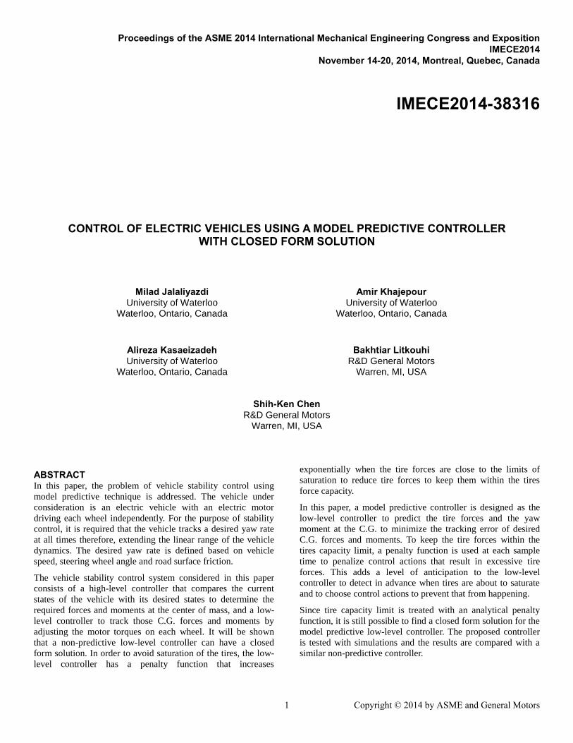
CONTROL STRUCTURE For a vehicle stability control system, a multi-layer control

structure is used. The control structure is shown in Figure 1. In

this figure, driver inputs are fed to the high-level controller.

This controller also receives information about the current

states of the vehicle and determines the target C.G. forces and

moments, F*CG, that can stabilize the vehicle. F*

CG is then

compared with the actual C.G. forces and moment, FCG, and the

optimal control action that minimizes the error E= F*CG -FCG is

determined in the low-level controller. The optimal control

action depends on the available actuators. In this study, it is

assumed that the only means of actuation is torque vectoring in

a four wheel drive vehicle. However, with only minor changes,

the controller can be applied to front/rear wheel drive vehicles.

Figure 1 Structure of the control loop.

CONTROLLER DESIGN

Non-Predictive Controller In the non-predictive low-level controller, the following

objective function is defined:

𝐽 = (𝑬 − 𝑨𝑓𝛿𝑭)𝑇

𝑾𝐸(𝑬 − 𝑨𝑓𝛿𝑭) + 𝛿𝑭𝑇𝑾𝑑𝑓𝛿𝑭

+ (𝑭 + 𝛿𝑭)𝑇𝑾𝐹(𝑭 + 𝛿𝑭) (1)

In Equation (1), E is the difference between the target and

actual C.G. forces and moments:

𝑬 = 𝑭𝑪𝑮∗ − 𝑭𝑪𝑮 = {

𝐹𝑥∗

𝐹𝑦∗

𝐺𝑧∗

} − {

𝐹𝑥

𝐹𝑦

𝐺𝑧 } (2)

Af is the Jacobian matrix that relates the change in tire forces to

the change in C.G. forces and moments. It can be defined as:

𝑨𝑓 = [

𝜕𝐹𝑥/𝜕𝐹𝐹𝐿 𝜕𝐹𝑥/𝜕𝐹𝐹𝑅

𝜕𝐹𝑦/𝜕𝐹𝐹𝐿 𝜕𝐹𝑦/𝜕𝐹𝐹𝑅

𝜕𝐺𝑧/𝜕𝐹𝐹𝐿 𝜕𝐺𝑧/𝜕𝐹𝐹𝑅

𝜕𝐹𝑥/𝜕𝐹𝑅𝐿 𝜕𝐹𝑥/𝜕𝐹𝑅𝑅

𝜕𝐹𝑦/𝜕𝐹𝑅𝐿 𝜕𝐹𝑦/𝜕𝐹𝑅𝑅

𝜕𝐺𝑧/𝜕𝐹𝑅𝐿 𝜕𝐺𝑧/𝜕𝐹𝑅𝑅

] (3)

F denotes tire longitudinal forces and δF stands for the change

in tire forces and moments:

𝑭 = [

𝐹𝐹𝐿

𝐹𝐹𝑅

𝐹𝑅𝐿

𝐹𝑅𝑅

] , 𝛿𝑭 = [

𝛿𝐹𝐹𝐿

𝛿𝐹𝐹𝑅

𝛿𝐹𝑅𝐿

𝛿𝐹𝑅𝑅

] (4)

WE and Wdf in Equation (1) are the weight matrices that are

tuned based on the trade-off between the tracking performance

(FCG*-FCG) and control effort (𝛿𝑭). The third term in Equation

(1) is a penalty term and is used to enforce tire forces to remain

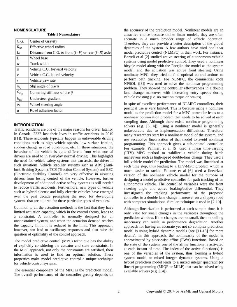
within the tire force capacity. The tire capacity ellipse is


illustrated in Figure 2. The radii of the ellipse are the maximum

force that the tire can generate in its longitudinal and lateral

directions and are approximated by:

𝐹𝑥 = 𝜇𝑥𝐹𝑧, 𝐹𝑦 = 𝜇𝑦𝐹𝑧 (5)

In this study, it is assumed that a separate estimation scheme is

available to provide estimates of the tire forces and the friction

coefficient at each tire.

Figure 2 Tire force capacity ellipse.

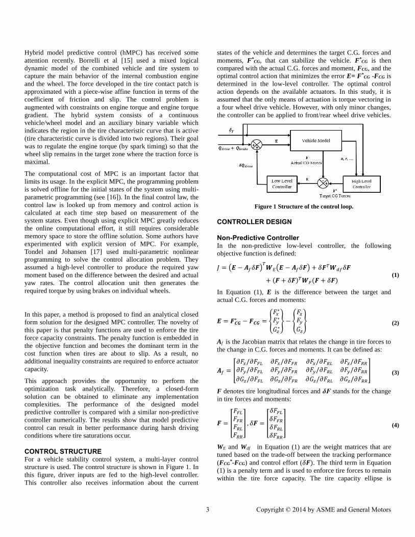
The weight matrix WF depends on actual tire forces and relative

margin to the borders of the capacity ellipse in Figure 2. The

goal is to ensure WF remains small when tire forces are well

within the tire capacity, and it grows when the tire is about to

saturate. To this aim, the variable ρij is defined as:

𝜌𝑖𝑗2 = (

𝐹𝑥,𝑖𝑗

𝐹𝑥𝑚𝑎𝑥

)2

+ (𝐹𝑦,𝑖𝑗

𝐹𝑦𝑚𝑎𝑥

)

2

(6)

with this definition, a polynomial function can be used to define

the diagonal elements of the WF matrix:

𝑤𝑖𝑗 = 𝛾(𝜌𝑖𝑗2 )

𝑛

𝑾𝐹 = 𝑑𝑖𝑎𝑔 [𝑤𝐹𝐿 𝑤𝐹𝑅 𝑤𝑅𝐿 𝑤𝑅𝑅] (7)

where 𝛾 and 𝑛 are chosen so that the weights rise relatively

rapidly as each tire saturates as shown in Figure 3.

Figure 3 The elements of WF weighting matrix.

The optimal control action 𝛿𝑭 can be obtained by minimizing

the cost function J in Equation (1):

𝜕𝐽

𝜕𝛿𝑭= 0 ⇒ 𝛿𝑭 = [𝑾𝐹 + 𝑾𝑑𝑓 + (𝑨𝑓

𝑇𝑾𝐸)𝑨𝑓]−𝟏

(𝑨𝑓𝑻(𝑾𝐸𝑬)

− 𝑾𝐹𝑭) (8)

Having calculated the optimal 𝛿𝑭, the corresponding amount of

change in the torque applied to each wheel can be calculated:

𝛿𝑄𝑖𝑗 = 𝑅𝑒𝑓𝑓𝛿𝐹𝑖𝑗 (9)

The dynamics of electric motors is much faster than vehicle

dynamics, because they have a very fast reponse time.

Therefore, it is safe to ignore their dynamics. In addition, since

the electric motor is capable of generating both positive and

negative torques, any sign for the optimal 𝛿𝑭 is acceptable.

MPC CONTROLLER DESIGN The non-predictive controller that was designed in the previous

section will be extended here to obtain the model predictive

controller. The cost function in Equation (1) will now include a

finite number of points in the future:

𝐽 = ∑(𝑬𝑘 − 𝑨𝒇𝛿𝑭𝑘)𝑇

𝑾𝑬(𝑬𝑘 − 𝑨𝑓𝛿𝑭𝑘) + 𝛿𝑭𝑘𝑇𝑾𝒅𝒇𝛿𝑭𝑘

𝑁

𝑘=1

+ (𝑭𝑘 + 𝛿𝑭𝑘)𝑇𝑾𝑭𝑘(𝑭𝑘 + 𝛿𝑭𝑘)

+ (𝛿𝑭𝑘 − 𝛿𝑭𝑘−1 )𝑇𝑾𝒔(𝛿𝑭𝑘 − 𝛿𝑭𝑘−1 )

(10)

where 𝑬𝑘, 𝑭𝑘 and 𝛿𝑭𝑘 denoted C.G. forces and moments error,

tire forces and control action at the kth instant of time,

repectively. The fourth term is optionally added to increase the

effect of future control actions 𝛿𝑭𝑘 (𝑘 = 2 … 𝑁) on the first

control action 𝛿𝑭1. Before the optimal control actions 𝛿𝑭𝑘 can

be calculated, 𝑬𝑘, 𝑭𝑘 terms need to be predicted. To this aim, a

prediction model is required. In this study, a linear double-track

vehicle model (Figure 4) is used to perform the predictions. The

prediction model developed here is a continuous model, but it

will be discretized with the sampling time. The prediction

model should provide an estimate of tire forces and C.G. forces

and moments in the prediction window. In the context of the

MPC, it is common to assume that the uncontrolled inputs (i.e.

steering wheel angle, brake and accelerator pedal positions)

remain constant throughout the prediction window. To make

this an acceptable assumption, the prediction window has to be

reasonably small.

Using cornering stiffness, the lateral tire forces can be

expressed as:

𝐹𝑦𝑖𝑗= 𝐶𝛼𝑖𝑗

𝛼𝑖𝑗, 𝑖 = 𝐹, 𝑅; 𝑗 = 𝐿, 𝑅 (11)

Assuming constant cornering stiffness, the rate of change of

lateral tire forces can be approximated by:


�̇�𝑦𝑖𝑗= 𝐶𝛼𝑖𝑗

�̇�𝑖𝑗 (12)

Considering only the effect of change in vehicle yaw rate, the

time rate of tire slip angles can be found as:

�̇�𝑖𝑗 =±

𝐿𝑖

𝑢

1 + (𝑣 ± 𝐿𝑖𝑟

𝑢)

2 �̇� (13)

Combining Equations (12) and (13), the change rate of tire

lateral forces can be found:

�̇�𝑦𝑖𝑗= 𝐶𝛼𝑖𝑗

±𝐿𝑖

𝑢

1 + (𝑣 ± 𝐿𝑖𝑟

𝑢)

2 �̇� (14)

Figure 4 Double-track vehicle model.

Therefore, having the current tire lateral forces (from a separate

estimation scheme), and calculating their time rate of these

forces using Equation (14), the future values of these forces can

be predicted.

Longitudinal tire forces are approximated as:

𝐹𝑥𝑖𝑗=

𝑄𝑖𝑗

𝑅𝑒𝑓𝑓

(15)

where Qij is the total torques exerted on the wheel ij. Writing

the balance of the moments acting on the vehicle gives:

(−𝑤

2𝑐𝑜𝑠𝛿𝑓 + 𝐿𝑓𝑠𝑖𝑛𝛿𝑓) 𝐹𝑥𝐹𝐿

+ (𝑤

2𝑠𝑖𝑛𝛿𝑓 + 𝐿𝑓𝑐𝑜𝑠𝛿𝑓) 𝐹𝑦𝐹𝐿

+

(𝑤

2𝑐𝑜𝑠𝛿𝑓 + 𝐿𝑓𝑠𝑖𝑛𝛿𝑓) 𝐹𝑥𝐹𝑅

+ (−𝑤

2𝑠𝑖𝑛𝛿𝑓 + 𝐿𝑓𝑐𝑜𝑠𝛿𝑓) 𝐹𝑦𝐹𝐿

+

−𝑤

2𝐹𝑥𝑅𝐿

− 𝐿𝑟𝐹𝑦𝑅𝐿+

𝑤

2𝐹𝑥𝑅𝑅

− 𝐿𝑟𝐹𝑦𝑅𝑅= 𝐼𝑧 �̇�

(16)

Equation (16) can be used to find the future values of vehicle

yaw rate and yaw moment.

Prediction of 𝑬𝑘 requires knowledge of 𝑭𝐶𝐺,𝑘∗ (i.e. future

outputs of the high-level controller). If this information is not

available, constant 𝑭𝐶𝐺,𝑘∗ assumption can be used. However,

estimation of 𝑭𝐶𝐺,𝑘∗ can significantly improve the performance

of the predictive controller.

In this study, since yaw stability is the main focus, 𝐺𝑧∗ is

predicted while 𝐹𝑥∗ and 𝐹𝑦

∗ are assumed constant in the

prediction window. A simple example of high-level control law

for yaw control is a proportional controller:

𝐺𝑧∗ = 𝑃(𝑟 − 𝑟𝑑) (17)

where P is the proportional gain and rd is the desired yaw rate

and is defined below:

𝑟∗ = 𝛿𝑓

𝑢

𝐿 + 𝑘𝑢𝑠𝑢2/𝑔

𝑟𝑑 = {

𝜇𝑔/𝑢 𝑟∗ > 𝜇𝑔/𝑢

𝑟∗ |𝑟∗| ≤ 𝜇𝑔/𝑢

−𝜇𝑔/𝑢 𝑟∗ < −𝜇𝑔/𝑢

(18)

The optimal control actions 𝛿𝑭𝑘∗ can be obtained by minimizing

the cost function in Equation (10) as:

𝜕𝐽

𝜕𝛿𝑭𝑘

= 0 ⇒

−𝑾𝑠𝛿𝑭𝑘−1 + (𝑨𝑓𝑇𝑾𝐸𝑨𝑓 + 𝑾𝑑𝑓 + 𝑾𝐹𝑘

+ 2𝑾𝑠)𝛿𝑭𝑘

− 𝑾𝑠𝛿𝑭𝑘+1 = 𝑨𝑓𝑇𝑾𝐸𝑬𝑘 − 𝑾𝐹𝑘

𝑭𝑘

(19)

Equation (19) comprises a set of linear algebraic equations that

can be solved to obtain 𝛿𝑭𝑘(𝑘 = 1 … 𝑁). Afterwards, 𝛿𝑭1 is

applied to the vehicle (using Equation (9)) and the rest are

discarded. This process is repeated at the next instant of time

with new measured signals. It can be seen that since penalty

functions are used to satisfy system constraints, no in-the-loop

optimization is required to find the optimal control action. This

significantly reduces the load on the processor.

SIMULATION RESULTS In this section, computer simulations in MATLAB Simulink

[18] are performed to evaluate the performance of the

predictive controller developed above. For the purpose of

simulation, CarSim software [19] is used to model a SUV

vehicle with properties listed in Table 2. The control loop

structure is the same as Figure 1, with the low-level controller

now being model predictive. The performance of the MPC and

Non-MPC controllers will be compared in two driving

maneuvers.


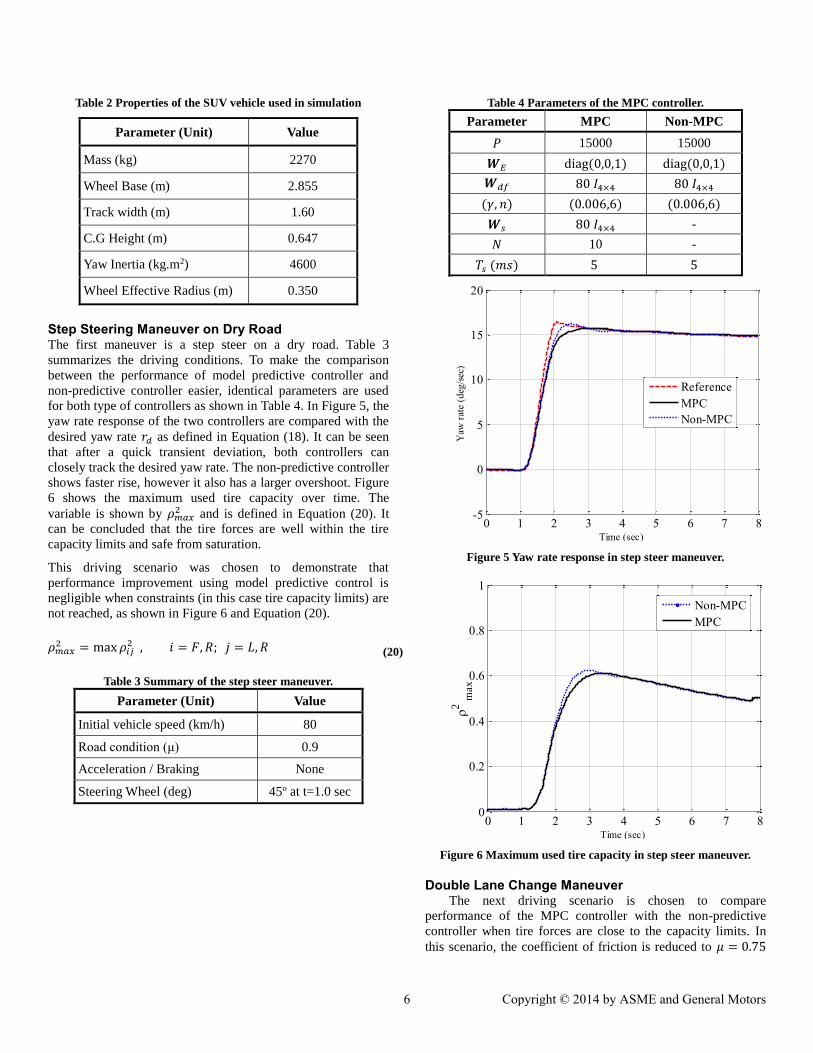
Table 2 Properties of the SUV vehicle used in simulation

Parameter (Unit) Value

Mass (kg) 2270

Wheel Base (m) 2.855

Track width (m) 1.60

C.G Height (m) 0.647

Yaw Inertia (kg.m2) 4600

Wheel Effective Radius (m) 0.350

Step Steering Maneuver on Dry Road The first maneuver is a step steer on a dry road. Table 3

summarizes the driving conditions. To make the comparison

between the performance of model predictive controller and

non-predictive controller easier, identical parameters are used

for both type of controllers as shown in Table 4. In Figure 5, the

yaw rate response of the two controllers are compared with the

desired yaw rate 𝑟𝑑 as defined in Equation (18). It can be seen

that after a quick transient deviation, both controllers can

closely track the desired yaw rate. The non-predictive controller

shows faster rise, however it also has a larger overshoot. Figure

6 shows the maximum used tire capacity over time. The

variable is shown by 𝜌𝑚𝑎𝑥2 and is defined in Equation (20). It

can be concluded that the tire forces are well within the tire

capacity limits and safe from saturation.

This driving scenario was chosen to demonstrate that

performance improvement using model predictive control is

negligible when constraints (in this case tire capacity limits) are

not reached, as shown in Figure 6 and Equation (20).

𝜌𝑚𝑎𝑥2 = max 𝜌𝑖𝑗

2 , 𝑖 = 𝐹, 𝑅; 𝑗 = 𝐿, 𝑅 (20)

Table 3 Summary of the step steer maneuver.


Initial vehicle speed (km/h) 80

Road condition (μ) 0.9

Acceleration / Braking None

Steering Wheel (deg) 45o at t=1.0 sec

Table 4 Parameters of the MPC controller.

Parameter MPC Non-MPC

𝑃 15000 15000

𝑾𝐸 diag(0,0,1) diag(0,0,1)

𝑾𝑑𝑓 80 𝐼4×4 80 𝐼4×4

(𝛾, 𝑛) (0.006,6) (0.006,6)

𝑾𝑠 80 𝐼4×4 -

𝑁 10 -

𝑇𝑠 (𝑚𝑠) 5 5

Figure 5 Yaw rate response in step steer maneuver.

Figure 6 Maximum used tire capacity in step steer maneuver.

Double Lane Change Maneuver The next driving scenario is chosen to compare

performance of the MPC controller with the non-predictive

controller when tire forces are close to the capacity limits. In

this scenario, the coefficient of friction is reduced to 𝜇 = 0.75

0 1 2 3 4 5 6 7 8-5

0

5

10

15

20

Time (sec)

Yaw

rat

e (d

eg/s

ec)

Reference

MPC

Non-MPC

0 1 2 3 4 5 6 7 80

0.2

0.4

0.6

0.8

1

Time (sec)

2 m

ax

Non-MPC

MPC


and the CarSim driver model is used to perform the double lane

change maneuver. The driving conditions for this scenario are

summarized in Table 5.

Table 5 Summary of the double lane change maneuver


Entry speed (km/h) 95

Road condition (μ) 0.75

Acceleration / Braking None

Steering Wheel Controlled by

driver

Driver preview time (sec) 1.50

Driver lag time (sec) 0.0

The yaw rate and side slip angle responses of the vehicle are

shown in Figure 7. In the upper graph, it can be seen that the

MPC controller (solid curve) is able to closely track the desired

yaw rate (dashed curve), while with the non-predictive

controller (dotted curve), vehicle becomes unstable after 𝑡 =5.5 𝑠𝑒𝑐. In the lower graph, the side slip angle of the vehicle is

shown. It can be observed that when the controller is not

predictive (dotted curve), the vehicle exhibits much larger side

slip angles especially after the second lane change. When MPC

controller is active, the side slip angle remains smaller than 4

degrees (𝛽 < 4𝑜).

Figure 7 Yaw rate and side slip angle in double lane change

maneuver.

In Figure 8, the maximum used tire capacity for each controller

is shown. Comparison between the two curves reveal that the

model predictive controller can keep the tire forces within the

capacity limits of the tires, whereas the non-predictive

controller is not able to avoid tire saturation. This is because the

MPC controller is able to anticipate the tire saturation in

advance and choose the proper control action so that the tire

saturation (and consequently vehicle skid) is avoided. Figure 9

shows the trajectory of the vehicle C.G. in each case. It can be

seen that the vehicle using non-predictive controller becomes

unstable after the second lane change.

Figure 8 Maximum used tire capacity in double lane change

maneuver.

Figure 9 Vehicle path in double lane change maneuver.

CONCLUSION In this paper, a model predictive controller was designed to

control the stability of electric vehicles. The designed controller

can be easily applied to front/rear and all wheel drive vehicles.

To obtain a closed-form solution for the MPC problem, tire

capacity limits were treated as a penalty function. A linear

double-track vehicle model was used to predict the vehicle yaw

rate and yaw moment as well as tire forces in the prediction

window. The performance of the designed controller was

compared with a similar but non-predictive controller. Through

computer simulations, it was observed that the performance of

0 1 2 3 4 5 6 7 8-40

-20

0

20

40

60

Yaw

rat

e (d

eg/s

)

0 1 2 3 4 5 6 7 8-30

-20

-10

0

10

Time (sec)

(

deg

)

Reference

MPC

Non-MPC

MPC

Non-MPC

0 1 2 3 4 5 6 7 80

0.2

0.4

0.6

0.8

1

Time (sec)

m

ax 2

MPC

Non-MPC

0 50 100 150 200 250-3

-2

-1

0

1

2

3

4

5

6

X (m)

Y (

m)

Non-MPC

MPC

Reference


the MPC controller is better than the non-predictive controller

in driving maneuvers that most of the tire force capacity is

needed.

ACKNOWLEDGMENTS The authors would like to acknowledge the financial support of

Automotive Partnership Canada, Ontario Research Fund, and

financial and technical support of General Motors.

REFERENCES

[1] Transport Canada, 2010, "Canadian Motor Vehicle Traffic

Collision Statistics," .

[2] Borrelli, F., Falcone, P., Keviczky, T., 2005, "MPC-Based

Approach to Active Steering for Autonomous Vehicle

Systems," International Journal of Vehicle Autonomous

Systems, 3(2) pp. 265-291.

[3] Gill, P., Murray, W., Saunders, M., 1998, "NPSOL–

Nonlinear Programming Software," Mountain View, CA, .

[4] Gill, P. E., Murray, W., and Saunders, M. A., 2002,

"SNOPT: An SQP Algorithm for Large-Scale Constrained

Optimization," SIAM Journal on Optimization, 12(4) pp. 979-

1006.

[5] Palmieri, G., Barbarisi, O., Scala, S., 2009, "A preliminary

study to integrate LTV-MPC Lateral Vehicle Dynamics Control

with a Slip Control," Decision and Control, 2009 held jointly

with the 2009 28th Chinese Control Conference. CDC/CCC

2009. Proceedings of the 48th IEEE Conference on,

Anonymous IEEE, pp. 4625-4630.

[6] Falcone, P., Tufo, M., Borrelli, F., 2007, "A linear time

varying model predictive control approach to the integrated

vehicle dynamics control problem in autonomous systems,"

Decision and Control, 2007 46th IEEE Conference on,

Anonymous pp. 2980-2985.

[7] Turri, V., Carvalho, A., Tseng, H., 2013, "Linear Model

Predictive Control for Lane Keeping and Obstacle Avoidance

on Low Curvature Roads," .

[8] Barbarisi, O., Palmieri, G., Scala, S., 2009, "LTV-MPC for

Yaw Rate Control and Side Slip Control with Dynamically

Constrained Differential Braking," European Journal of

Control, 15(3) pp. 468-479.

[9] Falcone, P., Borrelli, F., Tseng, H. E., 2008, "Linear

Time‐ varying Model Predictive Control and its Application to

Active Steering Systems: Stability Analysis and Experimental

Validation," International Journal of Robust and Nonlinear

Control, 18(8) pp. 862-875.

[10] Anwar, S., 2005, "Generalized Predictive Control of Yaw

Dynamics of a Hybrid Brake-by-Wire Equipped Vehicle,"

Mechatronics, 15(9) pp. 1089-1108.

[11] Camacho, E.F., and Alba, C.B., 2013, "Model predictive

control," Springer, .

[12] Morari, M., Baotic, M., and Borrelli, F., 2003, "Hybrid

Systems Modeling and Control," European Journal of Control,

9(2) pp. 177-189.

[13] Borrelli, F., Bemporad, A., and Morari, M., 2011,

"Predictive Control for Linear and Hybrid Systems," Prepation,

Draft Available at Http://Www.Me.Berkeley.Edu/Frborrel, .

[14] Cplex, I., 2007, "11.0 User’s Manual," ILOG SA,

Gentilly, France, .

[15] Borrelli, F., Bemporad, A., Fodor, M., 2006, "An

MPC/Hybrid System Approach to Traction Control," Control

Systems Technology, IEEE Transactions On, 14(3) pp. 541-

552.

[16] Pistikopoulos, E.N., Georgiadis, M.C., and Dua, V., 2007,

"Multi-parametric programming: theory, algorithms, and

applications," Wiley-VCH, .

[17] Tondel, P., and Johansen, T., 2005, "Control allocation for

yaw stabilization in automotive vehicles using multiparametric

nonlinear programming," Proceedings of the American Control

Conference, Anonymous Citeseer, 1, pp. 453.

[18] The Mathworks Inc., 2012, "MATLAB and Simulink

Toolbox," .

[19] Mechanical Simulation, 2011, "CarSim Users Manual," .


control of electric vehicles using a model predictive

Documents