control design risk assessment - virginia techmason/mason_f/cdra.pdfcontrol system design risk...

Control System Design

Risk Assessment

Using Fuzzy Logic

VPI - AOE - 239

Dr. Mark R. AndersonAssociate Professor

Department of Aerospace and Ocean EngineeringVirginia Polytechnic Institute and State University

October 1996

Foreword

The research and development reported here was accomplished for the Dynamicsand Control Branch of NASA Langley Research Center under grant NAG-1-1573.The NASA project engineer was Mr. Martin R. Waszak. The principal investigatorswere Dr. Mark R. Anderson and Dr. William H. Mason. Graduate studentsinvolved in the work included Mr. Valery Razgonyaev, Mr. Alexander Suchkov,and Ms. Chunhong Zhang. The research was performed during the period fromJanuary 1994 to January 1997.

The views and conclusions contained herein are those of the author and should notbe interpreted as necessarily representing the official policies or endorsements,either expressed or implied, of NASA Langley Research Center or any other agencyof the U.S. Government.

ii

Table of Contents

Introduction......................................................................................................................1

Short-Period Approximation........................................................................................2

Regions in the Complex Plane......................................................................................4

Design Requirements......................................................................................................9

Control System Design Strategies...............................................................................13

Fuzzy Logic Rules..........................................................................................................17

Examples..........................................................................................................................35

Suggested References....................................................................................................41

iii

The Table of Contents page is linked to the report sections. Select the Table of Contents entry to jump to the desired section.

Introduction

This manual describes a technique that can be used to assess the impact of theflight control system on aircraft configuration geometry. The primary purpose is toperform trade-off studies between different aircraft configurations in thepreliminary design phases of development. It can also be easily automated andadapted for use in aircraft configuration optimization problems.

The underlying approach is to determine the control system structure that isneeded to correct deficiencies in the dynamics of the aircraft. The complexity of thecontrol system is assumed to measure the amount of risk associated with thataircraft (if it were built). Configurations that require a very simple control systemarchitecture would incur only a small risk. Configurations with a very complicatedcontrol system would be assigned a higher risk.

The required control system architecture is determined using a set of fuzzylogic rules. These rules are developed using experience and knowledge about howcontrol systems are designed. Using this approach, a control system is not actuallydesigned for a given configuration under study. Only the required control systemstructure is determined. The final design of the control system would come afterthe final configuration has been selected and detailed aerodynamic and structuralmodels are developed.

This report describes a procedure and rulebase to determine the flight controldesign risk for the longitudinal axis of aircraft motion. Only one specificationregarding aircraft flying qualities is considered. However, the rules and methodsdescribed in this report could also be expanded to include other design requirementsand specifications.

1

Short-Period Approximation

The airplane will be modeled using the longitudinal, short-periodapproximation. This approximation assumes that the aircraft is flying at constantaltitude and speed. It is also based upon small angle assumptions and, therefore,cannot be used for rapid or highly dynamic flight trajectories. The equationsdescribing the short-period motion of a typical airplane are given by,

dα/dt = Zαα + q

dq/dt = Mαα + Mqq + Mδeδe

az = V(dα/dt - q)

where α is angle-of-attack, q is body-axis pitch rate, az is vertical acceleration, and δeis elevator deflection.

The parameters Zα, Mα, Mq, and Mδe are dimensional stability derivatives.The dimensional derivatives can be estimated using information about the aircraftgeometry and aerodynamics. Equations for the dimensional derivatives are,

Zα = - q- SCLαmV

Mα = q- ScCmα

Iyy

Mq = q- Sc2Cmq2IyyV

Mδe = q- ScCmδe

Iyy

where q- is dynamic pressure, c is chord length, S is wing reference area, m is mass,Iyy is a moment of inertia, and V is velocity. The terms CLα, Cmα, Cmq, and Cmδe arenon-dimensional aerodynamic derivatives. They must be estimated for eachaircraft configuration under study along with the geometric and weight variables (S,c, m, and Iyy).

By taking the Laplace transform of the equations above, the following transferfunctions can be obtained,

α(s)

δe(s) =

Mδe

s2 + 2bs + c

2

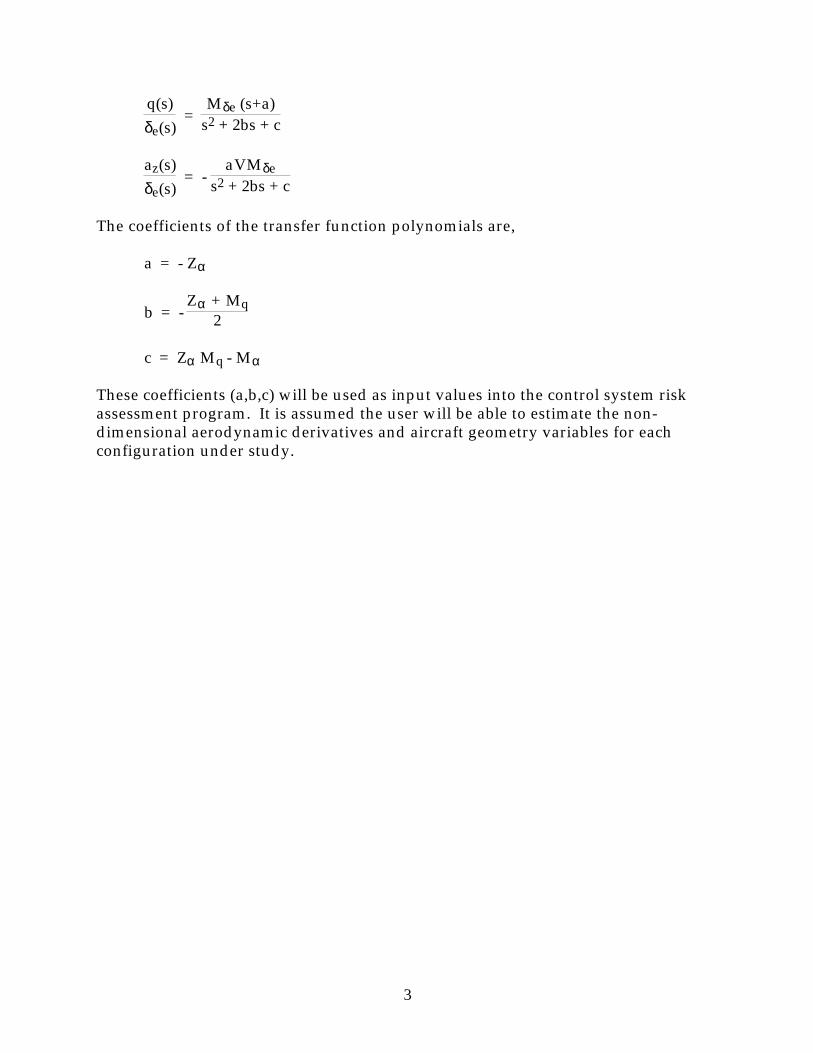
q(s)

δe(s) =

Mδe (s+a)s2 + 2bs + c

az(s)

δe(s) = -

aVMδe

s2 + 2bs + c

The coefficients of the transfer function polynomials are,

a = - Zα

b = - Zα + Mq

2

c = Zα Mq - Mα

These coefficients (a,b,c) will be used as input values into the control system riskassessment program. It is assumed the user will be able to estimate the non-dimensional aerodynamic derivatives and aircraft geometry variables for eachconfiguration under study.

3

Regions in the Complex Plane

In order to determine the control system that is required for a givenconfiguration, the characteristic roots of the bare-airframe must be analyzed. Thisanalysis consists of determining the region in the complex plane where the roots arelocated. With this information, one can then determine what control systemarchitecture that is needed to move the roots into the region specified by the designrequirements.

From the transfer functions listed previously, one finds the characteristicequation for the aircraft is given by the second-order polynomial,

s2 + 2bs + c = 0

The characteristic roots are the values of the Laplace variable s which satisfy thecharacteristic equation. Therefore, these roots are given by solutions to the quadraticequation above, or

s = -b ± b2 - c

The first situation to consider is to determine whether the characteristic rootsare complex or real. In the complex case, the discriminant is negative, i.e.

b2 - c < 0

Therefore, a test for complex roots can be completed using coefficients of thecharacteristic equation and the expression above. Namely, if b2 - c < 0 then the rootsare complex and if b2 - c > 0 then the roots are real

Two membership functions can be constructed to perform this test. Onemembership function indicates the presence of complex roots while the otherindicates the case of real roots. These membership functions are shown in Figure 1.

Membership functions are used to determine whether a particular input oroutput value belongs to, or is a member of, a given set. For the case depicted inFigure 1, all values of b and c leading to the result b2 - c < 1 belong in the "complex"set while all values of that lead to b2 - c > 1 belong to the "real" set. The utility offuzzy logic becomes apparent when one considers the case when b2 - c = 1.According to Figure 1, b2 - c = 1 belongs to both the "complex" and the "real" set.However, the membership functions also reveal b2 - c has membership of only 50%(0.5) in each of these sets. Thus, a "fuzzy" (rather than crisp) transition occurs asvalues pass from one set into another.

In this work, the equations used to represent the fuzzy logic membershipfunctions are called sigmoid functions. These functions have the form,

f(x) = 1

1 + e-α(x - β)

4

where α is the curvature and β is the center of the function. The "complex" set in

Figure 1 is represented by a sigmoid function with α = -10, β = 0. The "real" set is

represented by α = 10, β = 0.

-0.2

0

0.2

0.4

0.6

0.8

1

1.2

Deg

ree

of

Mem

ber

ship

-1 -0.5 0 0.5 1b*b-c

complex

real

Figure 1 Short-Period Pole Discriminant Membership Functions

We will also need to know if the roots are stable or not. Stable roots havetheir real part in the negative left-half-complex-plane. This test is easily performeduse Routh's stability criterion. The Routh stability test involves the signs of thecharacteristic equation coefficients. If all of the coefficients are positive, the rootswill be stable. If the coefficients change sign, the number of sign changes willindicate the number of right-half-plane (unstable) characteristic roots.

For the second-order case, we only need to consider the signs of thecoefficients b and c. However, keep in mind that the sign of the highest ordercoefficient (i.e. s2) dictates the start of the sequence. In this case, the sign of the s2

term is positive. There are four possibilities for the signs of b and c. When both band c are positive, there are no unstable roots. If the signs alternate with b < 0 and c> 0, then both roots will be unstable. Finally, only one unstable root will result ifeither b > 0 and c < 0 or b < 0 and c < 0.

Note than when c > 0, either both roots are stable or unstable. Thus, bothroots are together in either the left-half-plane or right-half-plane when c > 0. Whenc < 0, we have one stable root and one unstable root. As a result, the roots areseparated into the left-half-plane and right-half-plane when c < 0. We will thereforecreate a membership function based upon the sign of c to indicate whether the rootsare together or separate. This membership function is shown in Figure 2.

5

-0.2

0

0.2

0.4

0.6

0.8

1

1.2D

egre

e of

Mem

ber

ship

-1 -0.5 0 0.5 1c

split

together

Figure 2 Short-Period Pole Grouping Membership Functions

The sign of the coefficient b is closely related to system stability. Withcomplex roots, b > 0 indicates stable roots and b < 0 indicates unstable roots. This isnot a general statement on stability; however, as we have already noted that it ispossible to have one unstable root even though b > 0. Nevertheless, the sign of thecoefficient b will be used to represent stability. Positive values of b will indicatestable aircraft and negative values will indicate unstable aircraft roots. Amembership function describing this relationship is shown in Figure 3.

When the roots are real, we will need to know their location relative to theshort period zero of the pitch rate transfer function. This transfer function has onezero located on the real axis at s = - a. Since a is always positive, this zero is alwaysnegative and we know that it will lie to the left of the characteristic roots when theyare both unstable. The other possibilities are that the zero lies between the two realroots or to the right of the roots. Each case can be distinguished by the location ofthe zero to the nearest characteristic root. In terms of the characteristic equationcoefficients, the two real roots are given by,

6

-0.2

0

0.2

0.4

0.6

0.8

1

1.2D

egre

e of

Mem

ber

ship

-1 -0.5 0 0.5 1b

unstable

stable

Figure 3 Short-Period Pole Stability Membership Functions

s1 = - b + b2-c

s2 = - b - b2-c

The zero will lie to the left of the characteristic roots if - a < s2, or,

- a < - b - b2-c

or,

b - a < - b2-c

In the opposite case, the zero lies to the right of the roots if - a > s1, or,

- a > - b + b2-c

or,

b - a > b2-c

From these two expressions, we can see that the zero lies between the twocharacteristic roots if,

- b2-c < b - a < b2-c

7

Membership functions can be constructed to indicate the relative location ofthe pitch rate transfer function zero and the short-period characteristic roots. By

dividing the expression above by |b2-c|, the following inequality results,

- 1 < d < +1

where,

d = b - a

|b2-c|

Note that an absolute value is used to compute the parameter d. The absolute valueis used to insure that d is a real number even when the characteristic roots arecomplex. The parameter d then indicates the relative zero location. When d > 1,the zero is to the right of the roots and, when d < -1, the zero is to the left of theroots. When d lies between -1 and +1, the zero lies between the two characteristicroots. A membership function to represent this relationship is shown in Figure 4.

-0.2

0

0.2

0.4

0.6

0.8

1

1.2

Deg

ree

of

Mem

ber

ship

-2 -1 0 1 2d

left ofbetweenright of

Figure 4 Short-Period Zero Location Membership Functions

8

Design Requirements

Flight control systems are designed with several requirements in mind.Disturbance rejection, stability, command tracking, and ride comfort are some of therequirements that might be considered in the design. However, many of theserequirements only come into play when a detailed design is being considered.Usually a very high fidelity model of the aircraft is needed to determine if theserequirements are met or to implement a control system if the requirements are notmet.

Aircraft flying qualities are perhaps the most important requirements to beconsidered in the conceptual design stage. These requirements are determined bythe rigid-body dynamics of the aircraft and usually determine the basic structure ofthe control system that is required for the airplane. Certainly many final controlsystem designs far exceed the complexity of that needed to meet flying qualitiesrequirements, but the flying qualities requirements usually provide the foundationfor the start of the design.

For this report, only one flying qualities specification will be considered forthe longitudinal axis. This specification defines desired regions in the complexplane in which the characteristic roots must lie. This specification form isparticularly amenable to the fuzzy logic algorithm because the desired regions can beexpressed using membership functions.

The flying qualities specification considered herein is called the "ωspτθ2 and

ζsp" specification in MIL-STD-1797 (Flying Qualities of Piloted Aircraft, 28 June

1995). This specification involves the short-period natural frequency (ωsp), damping

ratio (ζsp), and pitch rate numerator time constant (τθ2). In terms of the transferfunction coefficients defined previously, we have,

τθ2 = 1a

ζsp = b

|c|

ωsp = |c|

Table 1 shows the "ωspτθ2 and ζsp" specification for three different flightcategories. Category A is for precision flying such as air-to-air refueling. Category Bis for cruising flight and Category C is for take-off and landing. The limits listed inTable 1 represent the Level 1 (satisfactory) regions for each flight category.

The specifications listed in Table 1 are the minimum level requirements thatmust be met. They are not necessarily the requirements that the flight controlengineer would design toward. In other words, the design objective might be toexceed the minimum requirements by some extent. Also shown in Table 1 is a"Design" entry. This row represents the design goals which one might attempt to

9

achieve in order to exceed the minimum specification requirements for all flightcategories.

Table 1 MIL-STD-1797 Short Term Pitch Flying Qualities Specification

Category ωspτθ2 ζsp ζsp ωsp 1/τθ2min min max min min

A 1.5 0.35 1.3 1.0 -B 1.0 0.30 2.0 - -C (Class I, II-C, IV) 1.2 0.35 1.2 0.87 0.38C (Class II-L, III) 1.2 0.35 1.2 0.70 0.28

Design 1.5 0.35 1.2 1.0 0.38

At first glance one might conclude that designing to exceed the minimumrequirements might lead to unnecessarily conservative designs. However, recallthat the purpose here is to evaluate control system design risk assessment at thepreliminary design stage. Consequently, only an approximate representation of thedesign requirements are needed.

Figure 5 shows the design goals plotted with respect to the aircraft shortperiod natural frequency and zero. Note that the design region is bounded by allthree requirements of these two parameters. In order to simplify the requirementsslightly (this eliminates one set of membership functions), the design goal for the

product of ωspτθ2 will be shifted upward. The shifted requirement is,

(ωsp - 0.43) τθ2 > 1.5

This shifting eliminates the requirement for ωsp > 1.0 rad/s because now all of the

configurations that meet the shifted ωspτθ2 requirement will also meet the ωsprequirement.

The short-period flying qualities design requirement can then be normalizedand written in the following forms,

e > 1 where e = 1

0.38τθ2

0 < f < 1 where f = ζsp - 0.35

0.85

g > 1 where g = (ωsp - 0.43) τθ2

1.5

10

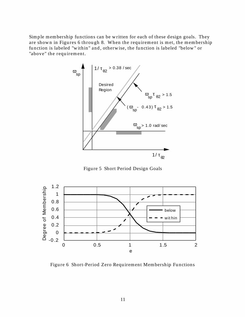
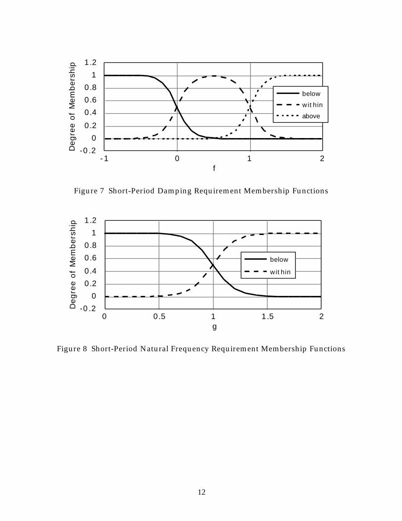
Simple membership functions can be written for each of these design goals. Theyare shown in Figures 6 through 8. When the requirement is met, the membershipfunction is labeled "within" and, otherwise, the function is labeled "below" or"above" the requirement.

ωsp

1/τθ2

1/τθ2> 0.38 /sec

ωsp> 1.0 rad/sec

ωsp

τ θ2 > 1.5

(ω - 0.43)sp

τ θ2 > 1.5

DesiredRegion

Figure 5 Short Period Design Goals

-0.2

0

0.2

0.4

0.6

0.8

1

1.2

Deg

ree

of

Mem

ber

ship

0 0.5 1 1.5 2e

below

within

Figure 6 Short-Period Zero Requirement Membership Functions

11

-0.2

0

0.2

0.4

0.6

0.8

1

1.2D

egre

e of

Mem

ber

ship

-1 0 1 2f

below

within

above

Figure 7 Short-Period Damping Requirement Membership Functions

-0.2

0

0.2

0.4

0.6

0.8

1

1.2

Deg

ree

of

Mem

ber

ship

0 0.5 1 1.5 2g

below

within

Figure 8 Short-Period Natural Frequency Requirement Membership Functions

12

Control System Design Strategies

There are six basic flight control system architectures that are used to controlthe longitudinal, short-period mode of a conventional aircraft. The control systemarchitecture that is needed for a given aircraft will depend on the dynamicproperties of the aircraft as well as the design requirements. These issues have beenaddressed in previous sections of this report, resulting in a description ofmembership functions that categorize both the properties of the aircraft and thedesign requirements.

The simplest possible control structure includes no feedback signals at all. Nocontrol system is required when the aircraft meets the design requirements withoutalteration. In this case, the aircraft can be flown satisfactorily without any stabilityaugmentation whatsoever. It is evident that very little flight control risk isencountered in this configuration so we will associate "low" risk with the case whenno feedback control is needed.

Probably the simplest stability augmentation scheme for the longitudinal axisis the pitch-rate-damper. This control system architecture assumes that the pitchrate gyro is used to measure aircraft body-axis pitch rate. These sensors are relativelyinexpensive and have been used for many years in the aircraft industry. However,although a pitch damper is not particularly sophisticated control system, it doesincur more risk than no control at all. Consequently, we will associate "medium"risk with a pitch damper design.

When designing a pitch damper, a simple gain is applied to the measure pitchrate and the product is added to the elevator command signal. The characteristicequation for the pitch damper controlled aircraft becomes,

1 + Kq Mδe (s+a)

s2 + 2bs + c = 0

Now consider the effect of the pitch damper gain Kq. When Kq is zero, thecharacteristic roots are given by the solution of s2 + 2bs + c = 0. This situation wasdiscussed previously for the open-loop airplane.

When Kq > 0, the root locus branches will migrate towards the pitch ratetransfer function zero located at s = -a. Since a is positive always, the tendency isthat the characteristic roots will increase damping as Kq is increased. As a result, thepitch damper is used primarily in the case when insufficient short-period dampingoccurs.

An accelerometer measures translational acceleration of the airplane. Thesedevices are also relatively inexpensive. An acceleration feedback signal structure isalso about as mature a technology as the pitch damper. Probably the only differencebetween the pitch rate and acceleration feedback is that the acceleration feedbackgain is more dependent on flight condition. This dependency means that theaccelerometer signal control system will involve more gain scheduling that thepitch damper. However, these are not insurmountable problems by any modern

13

means, so a "medium" control risk will also be associated with the accelerometerfeedback.

The characteristic equation resulting from accelerometer feedback is,

1 - Kaz aVMδe

s2 + 2bs + c = 0

Since the vertical acceleration transfer function has no zeros, the characteristic rootswill converge towards Butterworth patterns as Kaz is increased. The Butterworthpattern extends the root locus branches into the left-half-plane at constant anglesthat are symmetric about the real axis. Thus, the accelerometer signal feedback tendsto increase natural frequency (or the distance from the roots to the origin of thecomplex plane).

It is also possible to use both pitch rate and acceleration feedback signals. Inthis case, the characteristic equation becomes,

1 + Kq Mδe (s + (1-KqV/Kaz)a)

s2 + 2bs + c = 0

From this expression, we see that the closed-loop characteristic root loci will behavein a pattern similar to the pitch damper as Kq is increased. However, the zero ofattraction is now at s = - (1-KqV/Kaz)a rather than s = -a in the pitch damper case.With the blended feedback signal arrangement, the control system has the ability toplace this zero in a location such that the root locus branches behave as required.The blended arrangement is therefore very useful in correcting airplanes that aredeficient in both short-period damping and natural frequency.

It is worth noting at this time that the blended acceleration/pitch ratefeedback control architecture does not change the zero location of the pitch ratetransfer function. The blended feedback signals change the location of the "blended"zero which is neither the pitch rate or acceleration transfer function zero.Therefore, while this structure helps to improve short-period damping and naturalfrequency, it cannot be used to meet requirements on the pitch rate zero itself (i.e.

1/τθ2).Because the blended signal feedback requires at least two sensors and two

control system gains that are probably scheduled with flight condition, we willassociate at "high" control design risk with airplanes that need this control systemarchitecture.

The last control system configuration that will be considered is theproportional+integral control system. This system uses only a pitch rate sensor.The measure pitch rate is passed through a filter that includes a proportional gainand an integrator. The resulting filtered signal is then sent to the elevator to besummed with the pilot's input. The characteristic equation that results is,

14

1 + (Kqs + KI) Mδe (s+a)

s[s2 + 2bs + c] = 0

One can see from the characteristic equation above that the control system designercan now choose the location of the attracting zero arbitrarily. Also, an additionalpole exists that is located at the origin in the complex plane.

The proportional+integral controller architecture is very powerful design toolin that it can be used to stabilize aircraft with real unstable roots. Most staticallyunstable aircraft, or aircraft with aft center-of-gravity positions, need a controlsystem of this type.

Since the proportional+integral control system actually has dynamicelements in the control computer, it should be considered "very high" design risk.While it is indeed a powerful design tool, there are many practical design issues thatmust be addressed with this type of control system. For example, the integratorelement of the controller must be limited so that it does not "wind-up" when thecontrol surfaces reach their physical limits.

The last control system feature that is common in longitudinal axis designs isa trailing or leading edge flap schedule or augmentation controller. Because we may

have requirements on the location of the pitch rate zero a = 1/τθ2, some kind ofcontrol system may be required to change the location of this zero. As mentionedpreviously, this zero is computed from,

a = - Zα = qSCLαmV

From this expression, we see that the pitch rate zero depends upon the lift curveslope of the aircraft CLα. The most direct means of changing the lift curve slope is tochange the flap settings on the aircraft. Sometimes a flap schedule is used whileother times a feedback loop consisting of angle-of-attack feedback to the flaps is used.The flap schedule can be complicated because it may be scheduled as a function ofdynamic pressure, airspeed, or altitude. For a feedback augmentation scheme, areliable angle-of-attack measurement is needed. Regardless of the mechanization,the system usually requires accurate air data measurements. Therefore, we willconsider a flap augmentation scheme a "very high" control design risk.

Table 2 summarizes the application and risk associated with each of the sixcontrol system architectures. This information can be used to construct fuzzy logicmembership functions associated with each level of design risk. These membershipfunctions are shown in Figure 9. Note that each level of risk is assigned a numericalrange. For example, a "low" risk aircraft lies in the range of 0-25. These numericalranges are used so that one airplane can be easily compared to another. As such, thenumerical values assigned for risk cannot (at this time) be directly related to suchthings as component or life cycle cost. However, considering the complexity of thecontrol system as a significant factor in the cost of the control system developmentand implementation, it is reasonable to assume that at least some relationshipbetween cost and control risk exists.

15

Table 2 Control System Architectures and Risk

Control System Usual Application Risk

No Control Required Satisfactory Bare-Airframe LowPitch Damper Damping MediumAccelerometer Feedback Natural Frequency MediumBlended Signal Feedback Damping and Natural Frequency HighProportional+Integral Control Unstable Airplanes Very HighAugmented Flap Schedule Pitch Rate Zero Location Very High

-0.2

0

0.2

0.4

0.6

0.8

1

1.2

Deg

ree

of

Mem

ber

ship

0 25 50 75 100

Control Design Risk

lowmediumhighvery high

Figure 9 Control Design Risk Membership Functions

16

Fuzzy Logic Rules

This section describes each of the fuzzy logic rules that have been developedto assess flight control design risk for longitudinal-axis airplane models. Each rule islisted along with comments regarding the rule development. In particular, a rootlocus plot is shown in order to illustrate the control system structure that is neededto correct the flying qualities deficiency targeted by the particular rule.

The fuzzy logic rules are shown with the membership functions underlinedin each antecedent (the IF side of the rule). These membership functions refer tothose that were introduced in previous sections of this report. Also, the control riskassessment membership functions are underlined in the consequent (THEN side ofthe rule). The control risk membership functions were shown previously inFigure 9.

The fuzzy logic algorithm used for this work reports rules that are "fired"with the highest strength for each given configuration. The rules listed can betracked to the rule description given in this section. As a result, the user can tracethrough the rulebase to determine the deficiencies of a particular airplane as well asthe control system architecture needed to correct those deficiencies.

17

Rule 1: No Control Required

IF the short period poles are complex

AND the short period poles are stable

AND ωspτθ2 is within requirement

AND ζsp is within requirement

THEN control risk is low.

X

X

ORe

Im

ω sp, min

ζsp,min

Comments:

For this case, the open-loop aircraft dynamics already meet the design requirements.Therefore, at most, only control stick blending would be required and no aircraftresponse sensors are needed.

18

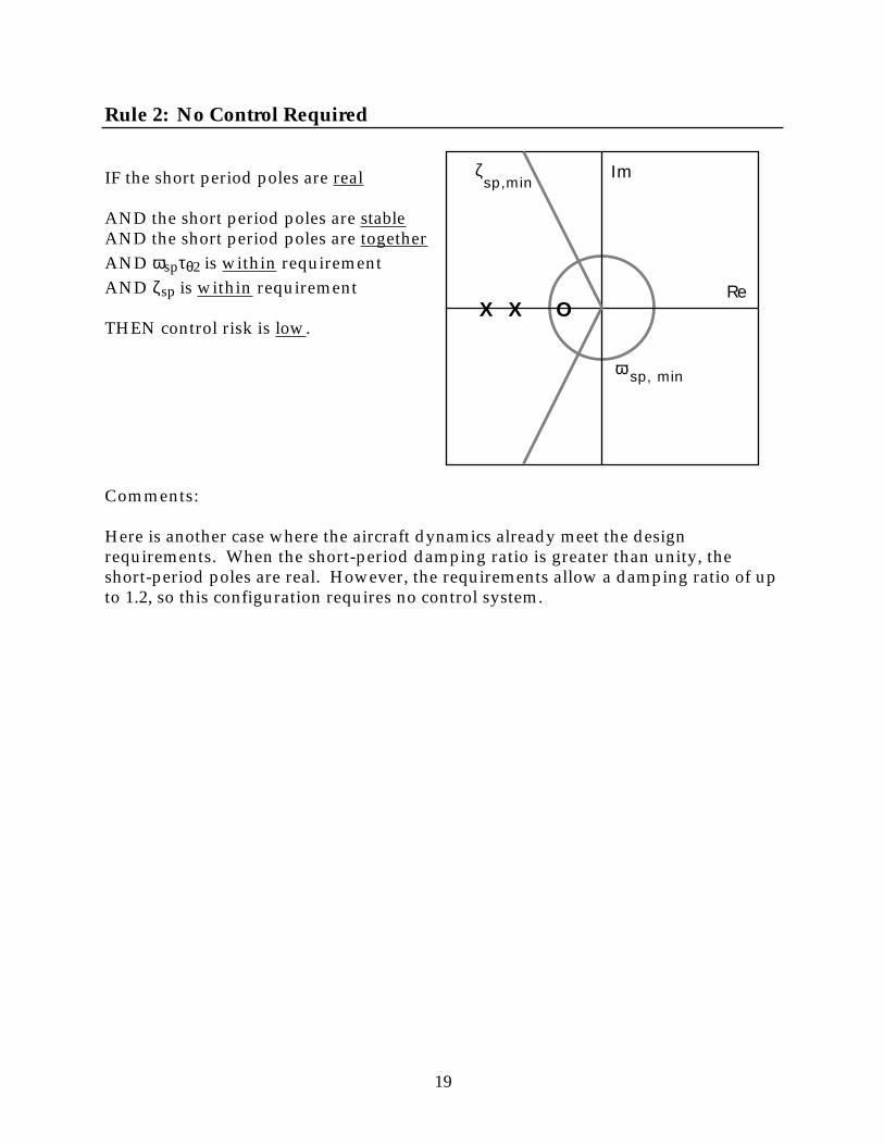
Rule 2: No Control Required

IF the short period poles are real

AND the short period poles are stableAND the short period poles are together



THEN control risk is low.XX O

Re

Imζsp,min

ω sp, min

Comments:

Here is another case where the aircraft dynamics already meet the designrequirements. When the short-period damping ratio is greater than unity, theshort-period poles are real. However, the requirements allow a damping ratio of upto 1.2, so this configuration requires no control system.

19

Rule 3: Pitch Damper




AND ζsp is below requirement

THEN control risk is medium.

X

X

ORe

Imζsp,min

ω sp, min

Comments:

This case depicts the classic use of a pitch rate damper to improve short-perioddamping ratio. The poles are complex and stable, but are located to the right of theminimum damping ratio boundary. Feedback of measured pitch rate to the elevatoror horizontal tail is required to fix this deficiency.

20

Rule 4: Pitch Damper


AND the short period poles are unstable


THEN control risk is medium.

X

X

ORe

Imζsp,min

ωsp, min

Comments:

It is also possible to stabilize and unstable configuration using a pitch damper. If theshort-period roots are complex and a located a sufficient distance from the origin, apitch damper can be used to move the closed-loop poles into the stable region of thecomplex plane.

21

Rule 5: Accelerometer Feedback



AND ωspτθ2 is below requirement


THEN control risk is medium.X

X

Re

Imζsp,min

ωsp, min

Comments:

When the short-period natural frequency is below the required minimum, anaccelerometer feedback to the elevator, canard, or horizontal tail surface can be usedto increase its magnitude. Because there is no zero in the acceleration transferfunction, an increase in the feedback gain will increase the effective closed-loopnatural frequency.

22




AND ζsp is above requirement


THEN control risk is medium.Re

Imζsp,min

ωsp, min

XX

Comments:

This root locus describes the rather unusual case where the short period dampingratio is too high. Pilots do not like the resulting deadbeat response because it leadsto rather abrupt accelerations. When the damping ratio exceeds the maximumvalue, the roots will be separated by a large distance on the real axis. Anaccelerometer can be used to reduce the damping ratio.

23




AND ωspτθ2 is below requirementAND the short period zero is right of thepoles

THEN control risk is medium.XX

Re

Imζsp,min

ω sp, min

Comments:

It is possible that the short-period roots are real, with damping ratio exceeding unity,but still have deficient natural frequency. In the case where the short period zero isstill to the right of the short period poles, the natural frequency can be increased atthe cost of a slight reduction in damping ratio. However, because the damping ratioalready exceeds unity, the reduction in damping ratio should be tolerable.

24

Rule 8: Blended Signal Feedback




AND ζsp is below requirement

THEN control risk is high.

X

X

ORe

Imζsp,min

blendedzero

ωsp, min

Comments:

In this case, the aircraft has deficient short-period damping and natural frequency.The remedy for this problem is to use a combination of pitch rate and normalacceleration feedback. This blending of two signals allows the designer to place azero in the complex plane so that the short-period roots are drawn into the requiredregion.

25



AND the short period poles are unstable


THEN control risk is high. X

X

ORe

Imζsp,min

blendedzero

ω sp, min

Comments:

When the short-period roots are complex, unstable, and close to the origin, it isdifficult to use only a pitch damper to move the roots into the required region.Therefore, a normal acceleration feedback blended with the pitch rate feedbacksignals so that the roots are not only drawn into the left-half-plane, but also drawnaway from the origin.

26



AND the short period poles are stableAND the short period zero is left of thepoles

THEN control risk is high. X XORe

Imζsp,min

blendedzero

ω sp, min

Comments:

When the short period poles are real, stable, and the short-period zero is to their left,the poles will have insufficient natural frequency. Because the short-period zero isto their left, a pitch damper could be used to improve natural frequency. However,most often the zero is too close to the poles and so acceleration feedback is needed tocreated a blended zero in the appropriate location far into the left-half-plane. As aresult, an combination of the pitch damper and accelerometer feedback is needed inthis situation.

27



AND the short period poles are unstableAND the short period poles are splitAND the short period zero is left of thepoles


Imζsp,min

blendedzero

ωsp, min

Comments:

In the case where one short-period pole is stable and the other is unstable, a pitchdamper can be used to draw both roots back into the left-half-plane provided thatthe pitch rate zero is left of the poles. In general, however, the zero has to be movedfarther into the left-half-plane to get closed-loop short-period roots with sufficientnatural frequency. A blend of normal acceleration and pitch rate feedback usuallyachieves the desired result.

28



AND the short period poles are stableAND the short period poles are splitAND the short period zero is left of thepoles


Imζsp,min

blendedzero

ωsp, min

Comments:

This is the same situation as described in Rule 11. This rule is needed to duplicateRule 11 because the split pole arrangement is possible with two different sequencesof characteristic equation coefficients.

29



AND the short period poles are unstableAND the short period poles are together

THEN control risk is high.

X XORe

Imζsp,min

blendedzero

ω sp, min

Comments:

A combination of normal acceleration and pitch rate feedback can also be used tostabilize the aircraft when both roots are unstable. The pitch rate zero will always beto the left of the roots in this case, but the location of the zero is probably insufficientto draw the closed-loop roots into the desired region. Consequently, the blendedzero is chosen to make the root locus branches act appropriately.

30

Rule 14: Proportional + Integral Control


AND the short period poles are stableAND the short period zero is betweenthe poles


THEN control risk is very high.X O

Re

Imζsp,min

XXOPI pole

PI zero

ωsp, min

Comments:

When the pitch rate zero lies between the two real short-period poles, it is notpossible to meet the necessary requirements with either the pitch damper oraccelerometer feedback, or both. The proportional+integral control structure allowsthe control system designer to place a real zero and an integrator pole in thecomplex plane. The pole and zero of the control system allow the root locusbranches to come together on the real axis before splitting into complex conjugatesin the desired region.

31



AND the short period poles are unstableAND the short period poles are splitAND the short period zero is betweenthe poles

THEN control risk is very high. X ORe

Imζsp,min

X XOPI pole

PI zero

ωsp, min

Comments:

A proportional+integral control structure is required when one short-period pole isunstable and the short-period zero is in-between the two poles. Theproportional+integral zero is placed to the left of the stable short-period pole. Thiscontroller zero tends to draw the closed-loop characteristic roots into the desiredregion of the complex plane.

32



AND the short period poles are stableAND the short period poles are splitAND the short period zero is betweenthe poles

THEN control risk is very high. X ORe

Imζsp,min

X XOPI pole

PI zero

ωsp, min

Comments:

This rule is the same as Rule 16. It must be included to account for the twocharacteristic equation coefficient sign sequences that lead to split unstable and stablepole configurations.

33

Rule 17: Flap Augmentation

IF short period zero is belowrequirement

THEN control risk is very high.

ORe

Im

(1/τ )θ2 min

Comments:

This rule covers the location of the short period zero. If the location of this zero isbelow its minimum required value, a flap schedule or flap augmentation feedback isneeded to move the zero above its minimum. Implementing an angle-of-attack toflap feedback controller is considered a "very high" risk control design.

34

Examples

The control system design risk assessment program has been implemented by

a group of macro files within in the MATLAB computer-aided engineeringenvironment. The five files needed to run the program are called: crisk.m,defuzzy.m, fuzrisk.m, fuzzy.m, and ruleval.m. They are included in the Appendix

of this report. None of the optional MATLAB toolboxes are needed to run theprogram. In fact, these files will also run without alteration on the student versions

of MATLAB.Consider, as an example, the XB-70 supersonic bomber. The stability

derivatives for this airplane when it is cruising at 40,000 ft, Mach 2.2 (supersonic) aregiven by:

Zα = - 0.52 (1/sec)

Mα = - 8.58 (1/sec2)

Mq = - 0.73 (1/sec)

Mδe = - 4.62 (1/sec2)

The transfer function coefficients are then computed as,

a = - Zα = 0.52 (1/sec)

b = - Zα + Mq

2 = 0.63 (1/sec)

c = Zα Mq - Mα = 8.96 (1/sec2)

The following text shows a sample run of the control system design riskassessment program. The user is asked to supply values of the pitch rate transferfunction coefficients a, b, and c. The program then computes the resulting controlsystem design risk. A list of rules is also printed to the screen along with theassociated strength of the rule as long as the strength of the rule is greater than 0.02.In the following example, the user input is specified by bold type.

The program is executed by starting the macro file called 'crisk.m' at the

MATLAB prompt.

»crisk

**************************************Control Design Risk Assessment Program**************************************

35

Please enter the numerator coefficient (a): 0.52

Please enter the denominator s1 coefficient (b): 0.63

Please enter the denominator s0 coefficient (c): 8.96

rules fired strength 3 0.8377 1 0.1622 17 0.0245

The final control design risk value is 34.55»

For this example, the final control design risk value predicted for the XB-70aircraft is about 35. This value means that the aircraft lies in the "medium" designrisk region. This value can be compared to other existing or prototype aircraft toyield a relative indication of increased or decreased design risk.

More information about the required aircraft control system can be obtainedby checking the rules that were fired that led to the predicted control risk value. Forthe XB-70 example, Rule #3 and Rule #1 fired with the highest strengths. Thestrength of a rule indicates to what degree the antecedents (left side) of the rule aretrue. Sorting through the rule descriptions discussed previously, we find that Rule#3 involves the case when the short period damping is low. A pitch damper controllaw (medium risk) is needed to correct this problem. Therefore, we know that thecontrol system of the airplane must have at least a pitch rate sensor and onefeedback gain.

Rule #1 fired with the second highest strength of 0.16. This rule is associatedwith the case where no control system is required. As a result, we can conclude thatthe short-period poles of the XB-70 in this flight condition are probably near theshort period damping ratio boundary. When the poles are near the boundary, bothRule #1 and #3 will fire and their relative strengths will indicate how close thepoles are to the boundary. For this case, the damping ratio of the XB-70 is 0.21 whilethe boundary is at 0.35. Since the damping ratio of the airplane is lower than therequirement, Rule #3 will fire with a higher strength than Rule #1.

The longitudinal control system for the XB-70 is shown in Figure 10. Notethat the control system includes a feedback of pitch rate to the elevator. This loopdemonstrates the pitch damper that is needed for high-speed flight. However, alsonote that the control system appears slightly more complicated than is predicted bythe control system design risk assessment method. The complexity of the finalcontrol system is under-predicted because we have only considered one flightcondition. The predicted control system design risk varies with flight conditionbecause the airplane stability derivatives vary with flight condition. The flightcondition that leads to the highest risk value will likely define the actual flightcontrol system architecture needed for the airplane.

36

lag

gainf(h)

gain

gain

gain

lead

gain

canard

elevator

pitch rate

normal accel

Mach number

normal accel (bobweight)

stick force

PA

clean

filter gain

Figure 10 XB-70 Longitudinal Control System

Consider a second flight condition of the XB-70, where the aircraft is cruisingat sea level, Mach 0.8 (subsonic). The stability derivatives of the airplane in this caseare:

Zα = - 1.19 (1/sec)

Mα = - 2.54 (1/sec2)

Mq = - 1.75 (1/sec)

Mδe = - 7.46 (1/sec2)

The transfer function coefficients are then,

a = - Zα = 1.19 (1/sec)

b = - Zα + Mq

2 = 1.47 (1/sec)

c = Zα Mq - Mα = 4.62 (1/sec2)

and the control system design risk is predicted by the following user input.

37

»crisk

**************************************Control Design Risk Assessment Program**************************************

Please enter the numerator coefficient (a): 1.19

Please enter the denominator s1 coefficient (b): 1.47

Please enter the denominator s0 coefficient (c): 4.62

rules fired strength 5 0.5908 1 0.4092

The final control design risk value is 27.89»

The subsonic flight condition leads to a "medium" design risk value of about28. This result is comparable to the supersonic case prediction of 34. However, notethat in the subsonic case, Rule #5 was fired with the highest strength. This rule isassociated with the need for an accelerometer feedback. Therefore, one can concludethat the pitch damper is needed for supersonic flight and an accelerometer is neededfor subsonic flight. This result explains the additional normal acceleration feedbackpath shown in Figure 10.

Several additional aircraft are analyzed in the following tables. These aircraftconfigurations can be used as a comparison to new prototypes or other existingdesigns.

38

Table 2 Control Risk for Large, High-Speed Aircraft

aircraft a b c Rules Fired Strength Risk

B-1 0.83 1.32 11.40 1 0.62 22.33 0.38

XB-70 (PA) 0.58 0.86 2.54 1 0.90 17.83 0.108 0.035 0.03

XB-70 (subsonic) 1.19 1.47 4.62 5 0.59 27.91 0.41

XB-70 (supersonic) 0.52 0.63 8.96 3 0.84 34.61 0.1617 0.02

SCAS (PA) 0.36 0.31 0.55 5 0.69 61.117 0.638 0.319 0.04

SCAS (high speed) 0.20 0.18 1.76 17 0.99 61.43 0.864 0.141 0.07

Table 3 Control Risk for Highly Maneuverable Aircraft


A-4D (PA) 0.82 1.20 11.49 1 0.51 24.73 0.49

A-4D 0.76 1.12 13.82 3 0.64 28.21 0.36

A-7 (PA) 0.73 0.65 3.10 1 0.56 27.83 0.448 0.105 0.10

39

A-7 1.09 1.00 9.92 3 0.59 27.21 0.41

F-4 0.53 0.64 8.15 3 0.81 33.61 0.18

F-18 0.39 0.38 2.01 3 0.72 47.917 0.431 0.284 0.02

X-29 (PA) 0.36 0.28 -3.00 16 0.94 87.517 0.6315 0.06

X-29 (high speed) 1.67 1.19 -34.6 16 1.00 87.5

Gripen 0.37 0.35 -6.49 16 0.97 87.517 0.5615 0.03

Table 4 Control Risk for Subsonic Commercial Aircraft


DC-8 (PA) 0.54 0.85 2.62 1 0.89 17.83 0.11

DC-8 0.68 1.04 5.76 1 0.73 19.93 0.27

Learjet M24 0.66 1.00 7.96 1 0.51 24.83 0.49

Boeing 747 0.52 0.58 1.54 1 0.60 31.35 0.408 0.203 0.2017 0.02

40

Suggested References

Anderson, M.R., Suchkov, A., Einthoven, P., and Waszak, M.R., "Flight ControlSystem Design Risk Assessment," AIAA Paper No. 95-3197, AIAA Guidance,Navigation, and Control Conference, Baltimore, MD, Aug. 1995.

Anderson, M.R. and Mason, W.H., "An MDO Approach to Control-Configured-Vehicle Design," AIAA Paper No. 96-4058, 6th AIAA/USAF/NASA/ISSMOSymposium on Multidisciplinary Analysis and Optimization, Sept. 1996.

Williams, T., "Fuzzy Logic is Anything but Fuzzy," Computer Design, April 1992,pp. 113-127.

Beaufrere, H. and Soeder, S., "Longitudinal Control Requirements for StaticallyUnstable Aircraft," 38th National Aerospace and Electronics Conference (NAECON),May 1986.

41

control design risk assessment - virginia techmason/mason_f/cdra.pdfcontrol system design risk...

Documents