control aspects of a diesel generator used to power a sodar device
TRANSCRIPT

Department of Mechanical Engineering
Control aspects of a Diesel Generator used to power a
SODAR device
Author: Ollie Kelleher
Supervisor: Dr. Matthew Stickland
A thesis submitted in partial fulfilment for the requirement of degree in
Master of Science in Renewable Energy Systems and the Environment
2010

Ollie Kelleher University of Strathclyde
MSc Renewable Energy Systems and the Environment 2010 i
Copyright Declaration
This thesis is the result of the author‟s original research. It has been composed by the author
and has not been previously submitted for examination which has led to the award of a
degree.
The copyright of this thesis belongs to the author under the terms of the United Kingdom
Copyright Acts as qualified by University of Strathclyde Regulation 3.50. Due
acknowledgement must always be made of the use of any material contained in, or derived
from, this thesis.
Signed: Ollie Kelleher Date: 10/09/2010

Ollie Kelleher University of Strathclyde
MSc Renewable Energy Systems and the Environment 2010 ii
Abstract
The main aim of this project was to apply control and functional operation to a diesel
generator that is used to charge batteries which in turn power a SODAR device. A
detailed literature review was conducted of the wind industry and current and
predicted wind measurement techniques used. The theoretical aspect of the SODAR
device was analysed.
The generator used as part of this project was inspected and maintenance was
conducted as necessary. The practical experimental aspect fell in line with the main
aim of the project. Preliminary laboratory work consisted of a detailed study and
understanding of a Campbell scientific data logger and then using it to perform basic
experimental measurements. Further application of the data logger led to the
acquisition of advanced software that was used to compile a program which
monitored the battery charge and the fuel levels of the generator. Alarm signals were
issued via a GSM modem in the event of certain conditions arising. The program was
applied by uploading it to the data logger and wiring it up accordingly such that all
input and output signals were detected as necessary.

Ollie Kelleher University of Strathclyde
MSc Renewable Energy Systems and the Environment 2010 iii
Acknowledgements
I would like to thank Dr. Matthew Stickland for all his help and guidance throughout
this project. Special thanks must also go to Franco Casule of Campbell Scientific who
was of great help in setting up the data logger used within this project. Also I would
like to thank other members of faculty for the assistance and supplying necessary
equipment throughout this project. They include Steven Black, John Redgate and Pat
McGuiness. Finally I would like to thank my family for their support and assistance
throughout this project and entire academic year.

Ollie Kelleher University of Strathclyde
MSc Renewable Energy Systems and the Environment 2010 iv
Table of Contents
Copyright Declaration .................................................................................................. i
Abstract ......................................................................................................................... ii
Acknowledgements .................................................................................................... iii
Table of Contents ........................................................................................................ iv
List of Figures ........................................................................................................... viii
List of Tables ................................................................................................................ x
Chapter 1: Introduction .............................................................................................. 1
1.1 Objectives of Report ............................................................................................ 1
Chapter 2: Background ............................................................................................... 2
2.1 Environmental Concerns ...................................................................................... 2
2.2 Oil Costs............................................................................................................... 4
Chapter 3: Wind Energy ............................................................................................. 5
3.1 History of Wind Energy ....................................................................................... 5
3.1.1 Large-Scale Generation of Electricity ........................................................... 7
3.2 U.K. and Wind Energy....................................................................................... 10
3.3 Problems associated with wind energy .............................................................. 12
3.4.1 Intermittency ................................................................................................ 12
3.4.2 Environmental Impacts ................................................................................ 12
3.4 Wind Energy Resource ...................................................................................... 14
Chapter 4: Measuring Wind ..................................................................................... 15
4.1 Measuring Wind in remote Locations................................................................ 15
4.2 LIDAR ............................................................................................................... 17
4.3 Satellite .............................................................................................................. 19
4.5 SODAR .............................................................................................................. 22

Ollie Kelleher University of Strathclyde
MSc Renewable Energy Systems and the Environment 2010 v
4.5.1 Introduction to SODAR ............................................................................... 22
4.5.2 History of SODAR ...................................................................................... 22
4.5.3 Theory of SODAR ....................................................................................... 24
4.5.4 SODAR Pulse Properties ............................................................................. 27
4.5.5 Calculating Wind Component from SODAR .............................................. 34
Chapter 5: Mobile SODAR unit ............................................................................... 36
5.1 Introduction ........................................................................................................ 36
5.2 SODAR device................................................................................................... 36
5.3 SODAR Deployment Considerations ................................................................ 38
5.3.1 Power availability ........................................................................................ 39
5.3.2 Weather Conditions ..................................................................................... 39
5.3.3 Data Acquisition .......................................................................................... 40
5.3.4 Remote Communication .............................................................................. 42
Chapter 6: Using the Data Logger ........................................................................... 43
6.1 Introduction ........................................................................................................ 43
6.2 Initial Retrieval .................................................................................................. 44
6.3 Powering the data logger ................................................................................... 44
6.4 Establishing Communication ............................................................................. 45
6.4.1 Setting up the apparatus ............................................................................... 45
6.4.2 Connecting to the Data Logger .................................................................... 45
6.5 Preliminary Programming .................................................................................. 46
6.5.1 Software description .................................................................................... 46
6.5.2 Program Tests .............................................................................................. 47
6.5.3 Preliminary Programming Results............................................................... 49
6.5.4 Discussion of Results ................................................................................... 49

Ollie Kelleher University of Strathclyde
MSc Renewable Energy Systems and the Environment 2010 vi
Chapter 7: Applying the Data Logger ..................................................................... 50
7.1 Introduction ........................................................................................................ 50
7.2 Engine Maintenance........................................................................................... 50
7.2.1 Replacing the battery ................................................................................... 50
7.2.2 Changing the Oil .......................................................................................... 51
7.2.3 Adjusting the throttle ................................................................................... 51
7.3 Control and Operation Requirements ................................................................ 51
7.4 Programming Software ...................................................................................... 52
7.4.1 LoggerNet 4.0 .............................................................................................. 52
7.4.2 Edlog ............................................................................................................ 53
7.5 Programming Description .................................................................................. 53
7.5.1 Introduction ................................................................................................. 53
7.5.2 Digital I/O Ports........................................................................................... 53
7.5.2 Flags............................................................................................................. 54
7.5.3 Run Generator.............................................................................................. 56
7.5.4 Output processing ........................................................................................ 56
7.5.5 Subroutines .................................................................................................. 57
7.6 Wiring the data logger ....................................................................................... 58
Chapter 8: Results and Discussion ........................................................................... 59
8.1 Introduction ........................................................................................................ 59
8.2 Laboratory experiments ..................................................................................... 59
8.3 Generator Repair ................................................................................................ 59
8.4 Data Logger Application.................................................................................... 60
8.4.1 Achieved Goals............................................................................................ 60
8.4.2 Identified issues ........................................................................................... 61

Ollie Kelleher University of Strathclyde
MSc Renewable Energy Systems and the Environment 2010 vii
Chapter 9: Conclusion and Recommendations ....................................................... 62
9.1 Conclusions ........................................................................................................ 62
9.2 Recommendations .............................................................................................. 64
References ................................................................................................................... 65
Appendix A: Prompt Sheet ....................................................................................... 67
Appendix B: Program Code ...................................................................................... 70
Appendix C: Wiring Diagram .................................................................................. 88

Ollie Kelleher University of Strathclyde
MSc Renewable Energy Systems and the Environment 2010 viii
List of Figures
Figure 1: World Primary Energy percentage Consumption by Fuel Type 2006 ........... 5
Figure 2: Early sail-wing horizontal-axis mill ............................................................... 6
Figure 3: First Large Windmill to generate electricity, Cleveland, U.S. ....................... 7
Figure 4: 200 kW Gedser Mill wind turbine, Denmark ................................................. 8
Figure 5: Increase in size of Wind Turbine designs over last 30 years. ........................ 9
Figure 6: Submitted and Consented wind farm applications in recent years. .............. 11
Figure 7: Wind Energy Resource Map for the U.K. .................................................... 14
Figure 8: SODAR and Anemometer measuring wind ................................................. 15
Figure 9: Doppler Lidar Wind Measurement Concept ................................................ 17
Figure 10: Inflow and wake wind LIDAR wind profile taken at the nacelle .............. 18
Figure 11: Typical measurement taken from LIDAR device ...................................... 19
Figure 12: SAR system viewing geometry .................................................................. 20
Figure 13: Map of Denmark showing SAR measured wind speed .............................. 21
Figure 14: Remtech arrayed SODAR .......................................................................... 24
Figure 15: Graphic description of Mechanical and Thermal Turbulance. ................... 25
Figure 16: Principle of SODAR shown with phased array .......................................... 26
Figure 17: Relationship between SODAR parameters ................................................ 29
Figure 18: Hanning Shape pulse frequency spectra for different ramp times ............. 32
Figure 19: Orientation of the SODAR beams .............................................................. 34
Figure 20: Internal view of SODAR device ................................................................ 37
Figure 21: Functioning Description of SODAR interface. .......................................... 37
Figure 22: CR10X data logger and wiring panel ......................................................... 40
Figure 23: Processes, Instructions and storage areas ................................................... 41
Figure 24: CR10X communication options ................................................................. 43

Ollie Kelleher University of Strathclyde
MSc Renewable Energy Systems and the Environment 2010 ix
Figure 25: Data logger and supply voltage .................................................................. 44
Figure 26: Screenshot of PC200W .............................................................................. 47
Figure 27: Preliminary data logger results ................................................................... 49
Figure 28: Logger Net user interface ........................................................................... 52

Ollie Kelleher University of Strathclyde
MSc Renewable Energy Systems and the Environment 2010 x
List of Tables
Table 1:Wind Energy Data .......................................................................................... 11
Table 2:SODAR internal components ......................................................................... 37
Table 3:Preliminary measurements logged .................................................................. 49
Table 4: Ports used on data logger ............................................................................... 54
Table 5:Flag description .............................................................................................. 55
Table 6:Final Storage data ........................................................................................... 56

Ollie Kelleher University of Strathclyde
MSc Renewable Energy Systems and the Environment 2010 1
Chapter 1: Introduction
1.1 Objectives of Report
The objectives of this report were as follows:
Literature Review
Conduct an investigation into factors that motivate research in wind energy.
Review the history of wind turbines and look at their evolution.
Identify the U.K.‟s position in relation to wind energy and the potential that lies in this
field for development and for the economy.
Develop an understanding of the funding that is available to subsidise capital costs
involved in this area of renewable energy and the initiatives undertaken by the U.K.
government to promote its development.
Identify some of the problems that are associated with wind energy on and off shore.
Look at existing methods of site surveying and measuring wind data for potential wind
turbine installations.
Look at the history of SODAR and its development to date.
Explain the detailed theory behind SODAR and exactly how it works.
Look at the mobile SODAR unit and identify some deployment considerations.
Data Logger control and operation
Understand the data logger operation and conduct preliminary test programming.
Explain control requirements of the mobile unit used to power SODAR.
Identify issues with the generator and conduct maintenance as necessary.
Describe the modifications, development and function of the program used to carry out
the control and operation of the generator and other components.
Highlight the outcome of the work conducted and recommend future work as
appropriate.

Ollie Kelleher University of Strathclyde
MSc Renewable Energy Systems and the Environment 2010 2
Chapter 2: Background
2.1 Environmental Concerns
There has been a great increase in the demand for renewable energy over the last decade
worldwide. World powers now acknowledge that fossil fuels are terminal and accept the need
for pre-emptive action. Significant steps were approved in the Kyoto treaty. This agreement
required participating countries to reduce greenhouse gas emissions to specified levels.
For the first five years of this century, 48% of total anthropogenic CO2 emissions remained in
the atmosphere. Effects include rising sea levels, glacier retreat, Arctic shrinkage, and altered
patterns of agriculture. Predictions for secondary and regional effects include extreme
weather events, an expansion of tropical diseases, changes in the timing of seasonal patterns
in ecosystems, and drastic economic impact. The evidence behind the climate altering effects
of greenhouse gas emissions is visible worldwide. Increased numbers of icebergs are
breaking away each day. It is estimated that arctic sea ice is melting at a rate of 9% per
decade. The International Panel on climate change predicts a mean global rise of 50cm in sea
level over the next one hundred years. In order to achieve the long-term stabilisation of the
atmospheric carbon dioxide concentration, the emissions will then have to be reduced by 56
percent by the year 2050 and approach zero towards the end of this century (Daily, 2010).
There are a number of possible solutions proposed to confront this problem:
Reduction of energy use (per person).
Carbon capture and storage.
Geo-engineering including carbon sequestration.
Population control, to lessen demand for resources such as energy and land clearing.
Shifting from carbon-based fossil fuels to alternative energy sources.
The latest report from the International Panel on Climate Change (IPCC) confirms that
hundreds of technologies are now available, at low cost, to reduce climate damaging
emissions, and that government policies need to remove the barriers to these technologies. It

Ollie Kelleher University of Strathclyde
MSc Renewable Energy Systems and the Environment 2010 3
is widely accepted that we cannot continue our current dependence on fossil fuels as a source
of energy.
The European Union has taken a lead by proposing aggressive targets for emission cuts.
A binding target to have 20% of the EU's overall energy consumption coming from
renewables by the year 2020 has been set. In the U.K., The 2007 White Paper: “Meeting the
Energy Challenge” sets out the Government‟s international and domestic energy strategy to
address the long term energy challenges faced by the UK, and to deliver 4 key policy goals:
1. To put the UK on a path to cut carbon dioxide emissions by some 60% by about 2050,
with real progress by 2020;
2. To maintain reliable energy supplies;
3. To promote competitive markets in the UK and beyond, helping to raise the rate
of sustainable economic growth and to improve productivity;
4. To ensure that every home is adequately and affordably heated.
(Government, 2007)
Implementing these solutions will enable people to usher in a new era of energy, one that
should bring economic growth, new jobs, technological innovation and, most importantly
environmental protection.

Ollie Kelleher University of Strathclyde
MSc Renewable Energy Systems and the Environment 2010 4
2.2 Oil Costs
Another factor that has caused interest in renewable energy is the rising price in oil around
the world. Oil accounts for 41% of the world‟s share of energy consumption. With oil
recently costing as much as $145 a barrel there is considerable demand for cheaper sources of
energy. As this is only likely to increase in the coming years our attention will turn initially
towards either nuclear or gas. These alternatives however, do not solve the long term problem
due to the negative effects that they too can have on our environment.
Historically, surges in oil prices have generated sporadic interest in developing alternative
energy sources including wind energy, which has proved to be the most commercially viable
renewable resource in the short term.
All research indicates that the demand for energy will only increase and with limited supply
of carbon based fossil fuels remaining it is essential that at least part of this demand is met
through renewable sources. An increasing amount of money is being put into renewable
energy research. The aim now is to develop reliable devices capable of providing a good
alternative to conventional energy sources.
Figure 1 displays the predicted energy consumption for each energy resource in quadrillion
British Thermal Units (BTU), (1BTU= 1055 J). For the next 30-40 years carbon based liquids
solids and gasses fossil fuels may continue to power the world, but the level of consumption
and the cost will continue to rise until finally it has all run out. Unless new oilfields are
discovered we will be left in a dark world.

Ollie Kelleher University of Strathclyde
MSc Renewable Energy Systems and the Environment 2010 5
Figure 1: World Primary Energy percentage Consumption by Fuel Type 2006
(EAI, 2010)
Chapter 3: Wind Energy
3.1 History of Wind Energy
Windmills were first developed for the use of grinding grain and pumping water. The earliest
known design is the vertical axis system developed in Persia about 500-900 A.D. Vertical axis
windmills were also used in China where they are thought to have originated. It is believed
that the first windmill was invented in China over two thousand years ago however the
earliest actual documentation of a Chinese windmill was in 1219 A.D.
The first windmills to appear in Western Europe were of a horizontal axis type. It is presumed
that the switch from vertical axis Persian design was due to the fact that European water
wheels had a horizontal configuration. They are also known to have had greater structural
stability.

Ollie Kelleher University of Strathclyde
MSc Renewable Energy Systems and the Environment 2010 6
As early as 1390, the Dutch set out to refine the tower mill design, shown in Figure 2, which
had appeared somewhat earlier along the Mediterranean Sea.
.
Figure 2: Early sail-wing horizontal-axis mill
(TelosNet, 2001)
It took over five hundred years to gradually improve the efficiency of the windmill sail design
as shown above. This process resulted in reaching a technological level which is now
recognised by modern designers and considered crucial to the performance of modern wind
turbine airfoil blades. Such advances include:
1. Camber along the leading edge,
2. Placement of the blade spar at the quarter chord position (25% of the way back from
the leading edge toward the trailing edge),
3. Centre of gravity at the same 1/4 chord position,
4. Nonlinear twist of the blade from root to tip.

Ollie Kelleher University of Strathclyde
MSc Renewable Energy Systems and the Environment 2010 7
3.1.1 Large-Scale Generation of Electricity
The first use of a large windmill to generate electricity was a system built in Cleveland, Ohio,
in 1888 by Charles F. Brush (Figure 3). The device was 17 meters in diameter.
Figure 3: First Large Windmill to generate electricity, Cleveland, U.S.
(TelosNet, 2001)
After World War I, the use of 25 kilowatt electrical output machines had spread throughout
Denmark, but cheaper and larger fossil-fuel steam plants soon put the operators of these mills
out of business.
Wind turbine development was enhanced by design improvements of aeroplane propellers and
monoplane wings. Some of the first early small electrical-output wind turbines in the 1900‟s
used modified propellers to drive direct current generators to produce electricity in remote
locations.
The first bulk power systems were developed in Russia in 1921, where they designed a
100kW Balaclava wind generator. The machine ran successfully for two years generating
200,00kWh of electricity. Further experimental wind turbines were undertaken around Europe
and the U.S after World War II as temporary shortages of fossil fuels drove research for
alternative solutions. Figure 4 shows the development towards a 3 blade structure that we are
familiar with today. This period of high energy costs is reflective of circumstances we see

Ollie Kelleher University of Strathclyde
MSc Renewable Energy Systems and the Environment 2010 8
today, however, global warming and carbon reduction had yet to become a priority.
Development continued worldwide until the 1960‟s when declining fossil-fuel prices once
again made wind energy uncompetitive with steam-powered generating plants.
Figure 4: 200 kW Gedser Mill wind turbine, Denmark
(TelosNet, 2001)
The 1980‟s again saw a resurgence in wind power R&D, largely driven by increased fuel
prices. Furthermore, in northern Europe countries such as Germany and Denmark were
beginning to leverage excellent wind resources to create a small, but stable market for
renewable energy organisations. Development was slow in the early 1990‟s as wind proved
uncompetitive with the likes of nuclear and fossil fuel based power generation. Increased
concern over global warming and government subsidisation increased interest, and with
technological advancement in the mid 90‟s and today, we see off shore structures with a
generation capacity in the region of 5MW. Figure 5 shows the evolution in size of wind
turbines over the past 30 years and the predicted generation capacity in the future with the

Ollie Kelleher University of Strathclyde
MSc Renewable Energy Systems and the Environment 2010 9
UPWIND project looking at development in the region of 10-20MW. In recent news from
Clipper Wind power, a 7.5 MW prototype is expected to be ready for production by
approximately 2012. This increase in size and capacity calls for accurate site surveying
techniques up to heights at which the device will be operational. Methods will be discussed
later in Chapter 4 (EWEA, 2010).
Figure 5: Increase in size of Wind Turbine designs over last 30 years.
(EWEA, 2010)

Ollie Kelleher University of Strathclyde
MSc Renewable Energy Systems and the Environment 2010 10
3.2 U.K. and Wind Energy
Renewable energy, and especially wind power, have had a significant impact on the British
power generation market in recent years and are targeted to deliver 20% of total supply by
2020. With this target in mind, we can expect to see an increase in contribution from
renewable resources in the near future. The UK has some of the richest renewable resources
in Europe, notably wind and marine (wave and tidal stream) resources. If they can be
harnessed effectively they can make a significant contribution to our long-term energy goals
relating to climate change and security of supply.
Recognising the potential benefits of renewable energy to the UK‟s energy objectives, in
2002 the Government introduced the Renewable Obligation Electricity Generation (RO) to
drive and support the growth of renewable energy generation. The Obligation allows
generally higher cost renewable electricity generation to compete directly with conventional,
fossil fuel based electricity generation. This obligation coupled with the proposed targets
spurred a rapid development of wind farms both on and off shore in the last decade. The
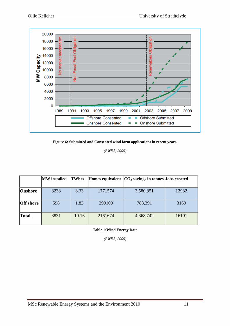
graph below (Figure 6) shows how the Renewable Obligation Certificates (ROC‟s) have
encouraged development in the wind industry which has simultaneously increased demand in
identifying potential sites and surveying and measuring data from them. Also shown in Table
1 is the installed wind energy capacity on and off shore, the contributing TW hrs for a
capacity factor of 29.4% onshore and 34.9% offshore, the number of homes that could be
supplied assuming an average annual household consumption of 4700kWh, the amount of
CO2 savings that took place with the replacement of brown energy with green (CO2 off set of
430 g/ kWh) and the estimated number of jobs created ( assuming 4 jobs are created in the
UK for each MW installed onshore and 5.3 jobs for each MW installed off shore according to
a report from Bain and Co) (BWEA, 2009).
Ollie Kelleher University of Strathclyde
MSc Renewable Energy Systems and the Environment 2010 11
Figure 6: Submitted and Consented wind farm applications in recent years.
(BWEA, 2009)
MW installed TWhrs Homes equivalent CO2 savings in tonnes Jobs created
Onshore 3233 8.33 1771574 3,580,351 12932
Off shore 598 1.83 390100 788,391 3169
Total 3831 10.16 2161674 4,368,742 16101
Table 1:Wind Energy Data
(BWEA, 2009)

Ollie Kelleher University of Strathclyde
MSc Renewable Energy Systems and the Environment 2010 12
3.3 Problems associated with wind energy
3.4.1 Intermittency
Wind energy production is intermittent and non-dispatchable. Effectively matching the supply
to the demand is often a problem. As discussed most turbines have a capacity factor of around
30%. Most renewable energy sources are tied to strong grids where the base load power plants
(generated by hydro-electric, coal or nuclear) minimise quality concerns and make it less
important for wind generation to be matched to consumption. Also Intermittency can be
balanced by using load management. This is when the load is adjusted or controlled rather
than the power station output. An example of load management in the UK is the night storage
heater, which is used to increase load overnight and therefore decrease the daytime load.
Another is wind energy with hydropower to ensure a backup resource.
An example such as Pumped-storage hydroelectricity means that energy generated at peak
output can be stored for times of high demand (ECORATER, 2010).There have also been
significant developments in battery storage over the last number of years, although batteries
are relatively expensive to use on a large scale.
3.4.2 Environmental Impacts
In Sweden, Denmark, the Netherlands and the UK a significant number of wind farms have
been installed both on and offshore. Their impacts will not be fully understood until
monitoring and research is conducted following their full installation. Placing wind farms
offshore eliminates some of the obstacles encountered when sitting wind farms on shore, such
as aesthetic impact on the landscape, annoyance to inhabitants from noise and flickering
light, conflicts with other planning interests etc.
Further challenges remain. For example, the impact off shore wind turbines may have on:
birdlife, marine life, hydrography and marine traffic. While there are now 20 years of
experience in assessing and meeting environmental challenges associated with land based
wind installations little is known of the effects of offshore wind installations.
Collection of information on existing sites, including the impacts on birds, flora and fauna,
sub-sea noise, visual intrusion, and coastal impacts will prove vital in the future of offshore
wind farm development and its environmental impacts (Peinke, 2007).

Ollie Kelleher University of Strathclyde
MSc Renewable Energy Systems and the Environment 2010 13
Birds
The biggest environmental effect that wind farms have is on birds. Such effects include:
• A physical change of the habitat providing extra resting areas.
• A collision risk for flying birds/bats
During periods with low visibility (darkness, fog, and heavy rain) there is a high probability
that flocks of birds could collide with a wind turbine if passing through a wind farm. The
tailwind that is produced by wind turbines also elevates the flight altitude and the migration
intensity of birds.
Suggestions have been made to use infrared cameras and microphones to study these effects
on bird life however it is not sure how successful they will prove to be.
There are atlases available that show the migrating routes for birds. These should be
consulted when considering the design and location of a wind farm. This will have an effect
on the future potential locations.
Studies have shown that wind turbines off shore can kill up to 10 birds per year. Again if it is
feared that some of those birds of migrating flocks are becoming endangered, planning
permission may become restricted in the future in some areas (MacKay, 2008).
Below the sea surface
Turbine foundations and the base supporting structure can have a serious impact on:
Hydrodynamic system,
Sediment characteristics,
Benthos composition (increase of epibenthos),
Fish fauna with possible implication to fisheries.
This can have a major impact on marine life in the surrounding waters and effect animals
such as seals, dolphins, fish etc. if changes in the marine ecosystem result in a variability of
the food chains.
There are other influencing factors such as:
Risk of ship collisions,
Sub-sea noise,

Ollie Kelleher University of Strathclyde
MSc Renewable Energy Systems and the Environment 2010 14
Interaction with outdoor recreational life and activities (surfing, sailing, kayaking etc.)
However the overall predicted impact in these cases is suspected to be less significant (Bruns,
2002).
3.4 Wind Energy Resource
The map in Figure 7 shows the annual mean wind speed in the U.K. Clearly Scotland and
Northern Ireland hold the best potential and therefore should exploit this resource as much as
possible. It is critical that turbines are located in the most suitable location in order to harness
maximum viability at the best cost. Such factors include the locality of transmission lines as
well as resource availability and consistency along with the environmental impact and
construction costs. Although off shore farms require higher initial capital investments to
construct, in the longer-term they may prove more environmentally friendly and more
economical due to their greater capacity.
Figure 7: Wind Energy Resource Map for the U.K.
(ECORATER, 2010)

Ollie Kelleher University of Strathclyde
MSc Renewable Energy Systems and the Environment 2010 15
Chapter 4: Measuring Wind
4.1 Measuring Wind in remote Locations
Wind power is moving towards the installation of wind farms in complex terrains, offshore,
in forests, and at higher altitudes. As discussed, wind turbines are now of multi MW capacity
and are ever growing. For this reason, there is increased demand for an improved
understanding of winds at these identified new challenging environments. Figure 8 shows the
difference in altitude measurement capabilities of a SODAR relative to an anemometer
mounted to a met mast.
Figure 8: SODAR and Anemometer measuring wind
(Oldbaum, 2010)
Traditionally, wind has been measured using cup anemometers mounted on metrological
masts however, with the increased height (Figure 8) and remoteness of turbines there may
not always be local masts for the site in question and the cost of erection and maintenance of
them has become more expensive. Furthermore, using an anemometer limits measurements to
one specific area of a turbine such as the centre of the rotor. There has been an increased need
for determining the wind over the whole turbine rotor as discrepancies have been identified

Ollie Kelleher University of Strathclyde
MSc Renewable Energy Systems and the Environment 2010 16
between the measured wind at the rotor centre and the turbine performance
(InternationalEnergyAgency, 2007).
In order to develop wind turbines on a potential site successfully, information should be
gathered and collected for each specific site. Such methods include LIDAR, Satellite, and
SODAR. By using remote sensing techniques wind profiles over the whole turbine can be
measured. Each various technique is based around the same principle of the Doppler shift and
they all hold particular advantages and limitations.
A recent development in the U.K. for remote sensing devices is the commissioning of the
first LIDAR and SODAR test site in August 2010 by one of the leading energy consultancy
companies; Natural Power. The site, located in Worcestershire has a 90m met mast which can
enable correlation reports to be made against ground based devices to provide traceability
back to anemometry. It is open to all developers, consultancies, research organisations and
turbine manufacturers (NaturalPower, 2010).
As this project was based around the use of a SODAR device other methods will only be
discussed briefly with more significant emphasis put on SODAR technology. Although most
of the following theory was not applied in the experimental aspect of this report it was felt
that it was of critical importance to comprehend it adequately due to the renewable nature of
this course.

Ollie Kelleher University of Strathclyde
MSc Renewable Energy Systems and the Environment 2010 17
4.2 LIDAR
LIDAR (Light Detection and Ranging) is an optical remote sensing technology that measures
properties of scattered light to determine wind speed and direction at significant heights using
the ground based device. It is similar to SODAR however it operates via the transmission and
detection of light rather than sound. The range to an object is determined by measuring the
time delay between transmission of a pulse and detection of the reflected signal. LIDAR is
believed to be most suitable to replace the met mast based wind measurements used in power
curve calculations for wind farms due to its level of accuracy in comparison to other methods.
LIDAR principle relies on measuring the Doppler shift of radiation scattered by natural
aerosols carried by the wind. Typically, these are dust, water droplets, pollution, pollen or salt
crystals. Figure 9 shows the principal on which LIDAR technology is based.
Figure 9: Doppler Lidar Wind Measurement Concept
(Gentry, 1999)
A new generation of fibre-based LIDARs has emerged over recent years that operates close
to the theoretical limit of sensitivity and typically only needs to detect one photon for every

Ollie Kelleher University of Strathclyde
MSc Renewable Energy Systems and the Environment 2010 18
1012
transmitted in order to measure wind speed. As the Doppler-shifted frequency is directly
proportional to line-of-sight velocity, the wind speeds obtained by LIDAR instrument seem
not to need calibration. This new technology which is available from companies such as
LIDAR wind technologies (Windcube) and Natural Power (ZephIR) is extremely portable
and can measure heights between 10m and 200m with acclaimed speed and direction
accuracy errors of less than 0.5% and 0.5° respectively. Similar to SODAR, LIDAR is also a
new instrument and its merits and limitations are not fully documented. In the case of the
LIDAR, the measurement of the wind speed takes place on the surface of a cone where the
depth changes as a function of the focus distance. It is believed that the LIDAR is the most
accurate remote sensing device and is most likely to completely replace met masts in terms of
absolute wind speed.
Research areas concerning LIDAR at the moment concentrates on two main topics, namely,
power curve assessment and wind field measurement from the nacelle. The first deals with
ground-based approaches to replace conventional anemometers mounted on a met mast. The
second aims at the development and verification of new nacelle-based approaches to measure
inflow and wake wind fields as shown below in Figure 10.
Figure 10: Inflow and wake wind LIDAR wind profile taken at the nacelle
(RenewableEnergyWorld, 2008)
Figure 11 shows low level jet observation measurements taken from a LIDAR device where
both wind speed and turbulence is recorded.

Ollie Kelleher University of Strathclyde
MSc Renewable Energy Systems and the Environment 2010 19
Figure 11: Typical measurement taken from LIDAR device
(InternationalEnergyAgency, 2007)
4.3 Satellite
Satellite remote sensing methods are based on microwave scatterometry and (SAR) Synthetic
Aperture Radar.
Satellite remote sensing provides wind maps 10m above sea level. The snap shot images are
produced twice daily and the wind maps are produced at a resolution of around 25km
therefore they are not immediately turbine site specific. Observations made by satellite
remote sensing are restricted to off shore and are as close as 40km distance to the shoreline.
Until recently satellites have not been used for offshore wind energy purposes even though
over 5000 observations have been taken at almost every location worldwide since 1999 to
date. The reason for this are:
satellite wind mapping accuracy
satellite wind mapping frequency
low resolution satellite wind maps do not include the coastal zone
technological methodologies to transfer satellite data to wind energy tools
SAR however, produces wind maps near coastal areas in which most wind farms are located.
The technology has been around since 1987 when the first Seasat carried the first SAR sensor
on board a satellite platform.

Ollie Kelleher University of Strathclyde
MSc Renewable Energy Systems and the Environment 2010 20
SAR operates by looking sideways between the angles from near range to far range (see
Figure 12). In this dimension, the slant range observations are made. The distance on the
ground between near and far range is the swath width. The across track resolution is obtained
through frequency modulation.
Azimuth range observations are made as the satellite travels along the flight track. The
azimuth resolution is specified as one-half the antenna length. The synthetic aperture is
obtained by tracking the individual phase and amplitude of individual return signals during a
given integration time interval. Hence the distance is much longer than the physical length of
the instrument antenna. It is the Doppler shift in each individual recorded signal in the
backscatter signal that determines the position of the scatter in the azimuth position (C.B.
Hasager, 2007).
The SAR illuminates a footprint and the signals returned from the footprint area are the
backscattered values, the NRCS (Normalised Radar Cross Section).
It is again the relationship between NRCS and ocean wind speed, similar to the
scatterometers, which is used to calculate the wind speed (C.B. Hasager, 2007).
Figure 12: SAR system viewing geometry
(C.B. Hasager, 2007)

Ollie Kelleher University of Strathclyde
MSc Renewable Energy Systems and the Environment 2010 21
As a resource though, it is not as reliable, as there are much fewer wind maps available (less
than 1000). By implementing statistical methods of few samples it is possible to obtain rough
estimates of the wind resource.
There is a known accuracy of around 1.1 m/s standard error on a series of wind maps in
comparison to offshore mast observations. This fact is particularly useful in determining and
identifying potential locations to install offshore masts (or LIDAR/SODAR devices). On top
of this if high quality met observations are available within a mapped area, the relative
differences in winds between different locations can be estimated with higher accuracy,
possibly around 0.6 m/s. Figure 13 below shows wind maps calculated from SAR.
Figure 13: Map of Denmark showing SAR measured wind speed
(InternationalEnergyAgency, 2007)
One limitation with satellite and SAR data is the fact that it is based on the wind stress at the
surface. For this reason there is a need to develop models to transfer this information to hub
height for a potential turbine site. This may not always be worthwhile and accurate enough.

Ollie Kelleher University of Strathclyde
MSc Renewable Energy Systems and the Environment 2010 22
4.5 SODAR
4.5.1 Introduction to SODAR
SODAR (Sonic Detection and Ranging) devices are used to remotely measure the vertical
turbulence structure and the wind profile of the lower layer of the atmosphere. This
technology has been widely used for meteorology applications however its usage in wind
energy, such as for measuring the wind field or the energy potential at a site, is relatively
new. SODAR systems are similar to radar except that it uses sound waves rather than radio
waves in the detection process. It is also similar to SONAR (Sound Navigation Ranging). The
main difference in this instance is the medium in which sound travels through. SONAR
systems detect the presence of objects underwater, while SODAR operates on the principal of
reflection due to scattering of sound by atmospheric turbulence (ART, 2008).
Some advantages of SODAR over other wind measurement techniques include:
Possibility to measure the wind profile over the whole rotor,
Ground based instrument makes it is faster, easier and cheaper to use relative to cup
anemometers mounted on met masts,
SODAR is generally cheaper than LIDAR.
Some drawbacks of SODAR include:
The limited experience in the use of the instrument,
Decrease in performance with height,
Dependence on the prevailing atmospheric conditions,
Need for a rigorous well established “absolute” calibration method.
(InternationalEnergyAgency, 2007).
4.5.2 History of SODAR
Acoustic scattering has been in development for the last 50 years. The primary reason for this
technology was to study the structure of the lower atmosphere. Like many new technologies
SODAR emerged from the United States during World War II. Here scientists used
acoustic backscatter in the atmosphere to examine low-level temperature inversions as they
affected propagation in microwave communication links.

Ollie Kelleher University of Strathclyde
MSc Renewable Energy Systems and the Environment 2010 23
It wasn‟t until the 1970's that the idea of designing acoustic sounders was seriously pursued
once researchers had shown experimentally that atmospheric echoes could reliably be
obtained to heights of several hundred meters.
The first two commercial systems were the Model 300 developed by AeroVironment and the
Mark VII developed by N.O.A.A. (National Oceanic and Atmospheric Administration). They
were used to measure the turbulent structure of the atmosphere up to several hundred meters.
The design of both devices was based around a parabolic dish and a facsimile recorder used
to provide an Analog record of backscatter data (ART, 2008).
The first digital based acoustic sounder was developed in 1975 at the University of Nevada at
Reno and at Scientific Engineering System, Inc. (S.E.S.). This was achieved by incorporating
a microcomputer into the system. Further developments from both S.E.S. and N.O.A.A. saw
the original single parabolic dish evolve into three axis digital based SODAR system which
was able to measure the Doppler shift and backscatter intensities in real time. This system
allowed the newly modified device to determine the vertical profile of the horizontal wind
speed and direction. This commercial Doppler system was made available in the late 1970‟s
by S.E.S. and was named Echosonde. By the early 1980‟s other companies such as Radian
Corporation were using the technological advancements that S.E.S. had made in Echosonde
as the basis for developing a microcomputer based three-axis Doppler SODAR system (ART,
2008).
The 1980‟s saw continued developments by various companies interested in improving this
technology. These include Xonics Inc. and AeroVironment Inc. as previously mentioned.
Xonic‟s device (Xondar), could measure wind profile and turbulence. AeroVironment‟s
Invisible Tower (AVIT) again was based on three adjacent parabolic dishes operating in
sequence however one was pointed vertically and the other two tilted 30 degrees from the
vertical in horizontally orthogonal directions (ART, 2008).
Outside of the U.S.A., other organisations in Europe and Australasia produced commercial
Doppler SODAR systems. One company in particular, Remtech in France, was one of the
first to commercialise phased array SODAR systems which were capable of measuring
Doppler shifts as well as turbulence parameters at heights of up to and over 1000 meters.
They were also the first company to apply multiple frequency coding which helped to extend
the altitude performance in SODAR. Figure 14 shows Remtech‟s arrayed Doppler SODAR
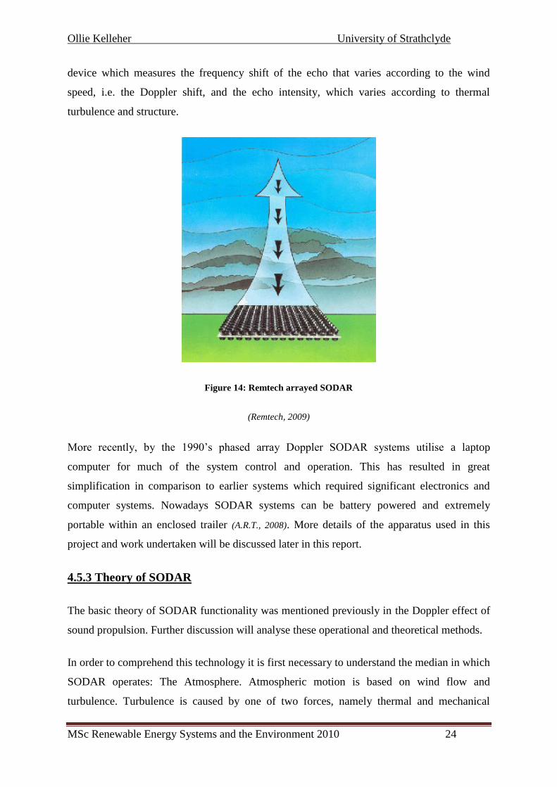
Ollie Kelleher University of Strathclyde
MSc Renewable Energy Systems and the Environment 2010 24
device which measures the frequency shift of the echo that varies according to the wind
speed, i.e. the Doppler shift, and the echo intensity, which varies according to thermal
turbulence and structure.
Figure 14: Remtech arrayed SODAR
(Remtech, 2009)
More recently, by the 1990‟s phased array Doppler SODAR systems utilise a laptop
computer for much of the system control and operation. This has resulted in great
simplification in comparison to earlier systems which required significant electronics and
computer systems. Nowadays SODAR systems can be battery powered and extremely
portable within an enclosed trailer (A.R.T., 2008). More details of the apparatus used in this
project and work undertaken will be discussed later in this report.
4.5.3 Theory of SODAR
The basic theory of SODAR functionality was mentioned previously in the Doppler effect of
sound propulsion. Further discussion will analyse these operational and theoretical methods.
In order to comprehend this technology it is first necessary to understand the median in which
SODAR operates: The Atmosphere. Atmospheric motion is based on wind flow and
turbulence. Turbulence is caused by one of two forces, namely thermal and mechanical

Ollie Kelleher University of Strathclyde
MSc Renewable Energy Systems and the Environment 2010 25
(Figure 15). A thermal turbulent force is caused by temperature differences in the
atmosphere (hot air raises causing wind currents). A mechanical turbulent force is caused by
air movement over natural or man-made obstacles. This interactive mechanical turbulent
force is due to the earth‟s rough variation in surface smoothness and is less prominent over
flat seas. The impact of turbulence from both mechanical and thermal sources is the
formation of eddies. In the case of mechanical turbulence the size of the eddy is directly
proportional to the size of the obstruction and speed of the wind.
Figure 15: Graphic description of Mechanical and Thermal Turbulance.
(Buck, 2008)
When a sound pulse, is transmitted from the SODAR device through the atmosphere it meets
an eddy and its energy is then scattered in different directions (See Figure16). The scatter
pattern that thermal and mechanical turbulence produce is different. However, there is almost
always a proportion of acoustic energy reflected back towards the source of sound. This
backscatter or atmospheric echo is then measured using a monostatic SODAR system.
Logically, as the acoustic pulse is reflected as backscatter the angle between the eddies and
the antenna is 180° as it returns directly towards the source. This detected backscatter is only
caused by thermally induced turbulence and mechanical turbulence is generally not detected
in a monostatic system (ART, 2008).

Ollie Kelleher University of Strathclyde
MSc Renewable Energy Systems and the Environment 2010 26
Figure 16: Principle of SODAR shown with phased array
(SCINTEC, 2004)
Bistatic SODAR systems have transmitting and receiving antennas at various locations.
Because of this scattering angles other than 180° can be detected. As well as that, the increase
in range of angles allows both thermal and also mechanical turbulence to be picked up. It also
increases the complexity of the device in design and application.
The shift in frequency of the returned signal relative to the frequency of the transmitted signal
is thanks to the Doppler Effect as discussed. It is this difference that allows us to calculate the
measure of air movement at the position of the scattered eddy. If the target or reflected
turbulent eddies are moving in the direction of the SODAR antenna, it will have a higher
frequency than that of the transmitted signal. The opposite also applies in that when the target
is moving away from the antenna, the returned frequency will be lower. It is this
characteristic that allows Doppler SODAR systems to measure atmospheric winds and
turbulence.
The thermal structure and radial velocity of the atmosphere at varying distances from the
transmission antenna can be determined by measuring the intensity and the frequency of the
returned signal as a function of time after the transmitted pulse. By sending consecutive
pulses, one in the vertical and two in orthogonal directions at angles slightly tilted from the
vertical we can obtain even further information. This can be done by conducting geometric

Ollie Kelleher University of Strathclyde
MSc Renewable Energy Systems and the Environment 2010 27
calculations to obtain vertical profiles of the horizontal wind direction and both horizontal
and vertical wind speeds (ART, 2008). Some of these calculations will be looked at later in
Section 4.5.5, however, first it is important to understand the transmitted pulse properties and
some of its influencing factors.
4.5.4 SODAR Pulse Properties
A Transmitted sound pulse that is delivered by SODAR is scattered by fluctuations of the
refractive index of air and by eddies as discussed. Other factors that cause these fluctuations
include variation in temperature and humidity of the air as well as wind shear.
Turbulent fluctuations move with the wind. Therefore, the Doppler Effect shifts the sound
frequency during the scattering process. This level of frequency shift is proportional to the
velocity of the scatter in the beam direction. For example, if the beam is directed vertically,
the vertical wind speed w can be calculated directly from the Doppler shift. In order to
calculate the horizontal components it is necessary to tilt the beam also by a small angle θO
from the vertical into two horizontally perpendicular directions whose wind components can
be named u (East) and v (North). Now three Doppler shifts are obtained from each
transmitted pulse, which are a function of the wind components u, v, and w (Ioannis Antoniou,
2003).
The transmitted pulse is assumed to be confined to a conical beam of half-angle θ. For a
system having pulse duration τ and with speed of sound c, the pulse is spread over a height
range of cτ. As the pulse is scattered, it is detected at any one time from a volume (V) where:
Equation 1: Volume of pulse detected
2( )2
cV z
Where 2
c is the height range and
2( )z is the horizontal extension with z being the height above
the antenna array.
The ratio between received and transmitted powers at a height of a 100 m above ground and
for a 4500 Hz SODAR is typically of the order of 10-14
Therefore absorption in the
atmosphere is an important factor restricting the range that is the maximum height from

Ollie Kelleher University of Strathclyde
MSc Renewable Energy Systems and the Environment 2010 28
which scattered signals can be detected. The ratio of received to transmitted power is
proportional to the absorption term as shown in Equation 2:
Equation 2: Ratio of Received to Transmitted Power Proportional to Absorption
2 zR
T
Pe
P
Where the absorption coefficient α is the sum of classical absorption, αc, and molecular
absorption, αm. Classical absorption is due to viscous losses when sound causes motion of
molecules, and is proportional to frequency squared. Molecular absorption is due to water
vapour molecules colliding with oxygen and nitrogen molecules and exciting vibrations,
which are dissipated as heat. At low humidity there is little molecular absorption (Ioannis
Antoniou, 2003). At high humidity O2 and N2 molecules are fully excited without acoustically
enhanced collisions, and there is again little extra absorption. Absorption also depends on
temperature and pressure since these affect collisions. The resulting equation shows a
complicated dependence on the mentioned parameters as well as on the sound frequency.
However, in the frequency range of interest for SODARS that is between 1 and 10 kHz the
following rule is valid: The higher the frequency of a SODAR the more limited its range due
to absorption (Salomons, 2001).
Sending Beam signal
Parameters that effect how the SODAR sends the beam include:
1. Transmit frequency (fT)
2. Transmit power (PT)
3. Pulse length (τ)
4. Rise time (up and down) (βτ)
5. Time between pulses (T)
6. The tilt angle

Ollie Kelleher University of Strathclyde
MSc Renewable Energy Systems and the Environment 2010 29
Some of these parameters and the relationship between them are shown in Figure 16. Shown
is the basic pulse shape emitted from one transmitter and the repeated pulse with a time
interval between. A brief description of each parameter and its effects follows.
Figure 17: Relationship between SODAR parameters
(Ioannis Antoniou, 2003)
Frequency
The frequency of a standard phased array SODAR is decided in the design process and
cannot be altered much once assembled. Choosing the frequency is based on two factors,
overcoming background noise and absorption in the atmosphere. Because absorption also
depends on temperature (T) and relative humidity (RH), the frequency must be chosen
carefully as it is the only independent design parameter.
Power
The most important factor relating to power is to make sure the speakers are not damaged by
the voltage signal. This can be clearly seen from the SODAR equation:

Ollie Kelleher University of Strathclyde
MSc Renewable Energy Systems and the Environment 2010 30
Equation 3: SODAR equation, Power received.
2
22
z
R T e s
c eP P GA
z
RP = Power received from the atmosphere
TP = Transmitted power
G = Antenna transmitting efficiency
eA = Antenna effective receive area
= Pulse length
z = Height
α = Absorption of air
s = Turbulent scattering cross section
c = Wind speed in air (± 340 m/s)
If more power is put into the beam, more power will be received back. For this reason it is
necessary to consider how much power the speakers are able to deliver without being
damaged (Ioannis Antoniou, 2003).
Pulse length
The pulse length is the length of the pulse as shown in Figure 17. It is measured in
milliseconds or in meters. The effective pulse width with respect to power output is used in
calculations. This is the pulse width without the rise time plus half the rise time (up and
down). So a pulse length of 100 ms with a rise time (up and down) of 15% will have an
effective pulse length of 85 ms.

Ollie Kelleher University of Strathclyde
MSc Renewable Energy Systems and the Environment 2010 31
The pulse length has an impact on the following parameters:
1. Power received from the atmosphere,
Looking again at Equation 3 it can be seen that a longer transmit pulse means more received
power.
Equation 4: Pulse width is proportional to received power.
R
T
P
P .
2. Frequency resolution,
Equation 5: Relationship between frequency and Pulse length
1Vf
3. Height resolution,
Equation 6: Relationship between height and pulse length
2
cz
Rise time
The reason that there is a rise time in the signal is because it passes through a Hanning filter
first. This gives the signal a ramp up and down at the beginning and the end and helps to
protect the speakers from too quick a rise in voltage, which could cause them harm (Ioannis
Antoniou, 2003).

Ollie Kelleher University of Strathclyde
MSc Renewable Energy Systems and the Environment 2010 32
By assuming a pulse shape p(t) and duration τ, determining the Hanning shape is defined as
follows:
Equation 7: Calculating Hanning shape
The frequency spectra for three pulse shapes are shown in Figure 18 below.
Figure 18: Hanning Shape pulse frequency spectra for different ramp times
(Ioannis Antoniou, 2003)
For an ideal pulse β=0, all the energy would be in the main lobe of the sine function around
the y-axis and decay to zero with no ripples. This is not practical as unwanted ripples are
introduced to the frequency. By increasing β, the pulse becomes broader and deeper with
fewer ripples due to more of the energy being in the main lobe. This is a more desired effect,
however broadening the main lobe causes the transmit frequency to be less well defined, for
this reason a balance must be reached between ripples, pulse power and a well defined
transmit frequency.

Ollie Kelleher University of Strathclyde
MSc Renewable Energy Systems and the Environment 2010 33
Time between pulses
Time between pulses and the maximum height the SODAR attempts to measure have a direct
relationship. It is critical that any measure of backscatter must be finished before the next
pulse is sent therefore the maximum height is cT/2.
For phased array SODAR it is important to make sure backscatter from other pulses have
been completely detected before sending out another pulse, otherwise it could effect the
measurements and have an undesired effect.
The Tilt Angle
The tilt angle θ is defined by the loud speaker spacing d of the antenna array, by the number
of speakers N and by the transmit frequency f (or wave number k). The resulting intensity
pattern can be compared to optical interference patterns:
Equation 8: Intensity of loudspeaker array of N speakers
2
sin sin2
sin sin2
dNk
Id
k
In theory it is possible for the beam to be steered by a variable phase-shift between 0 and π/2
between two respective loudspeaker groups. Manufacturers of SODAR fix the progressive
phase-shift at π/2, which helps to simplify the design. In practice this leads to tilt angles of
16° - 30° for higher to lower transmit frequencies respectively. The practical limit on the
beam tilt angle is:
Equation 9: Limit on beam tilt angle
2
4tilt
dk
(Ioannis Antoniou, 2003)

Ollie Kelleher University of Strathclyde
MSc Renewable Energy Systems and the Environment 2010 34
4.5.5 Calculating Wind Component from SODAR
Having reviewed some of the parameters of the signal beam, it is important to understand
how the returned signal is used to calculate relevant wind data. If three beams w,v and u, as
described in section 4.5.4 were sent into the atmosphere the returned scatter data can be
analysed. The signal transmitted from a SODAR is a travelling wave with components like
sin(ωt-kz) or cos(ωtkz). The sound wave is scattered by turbulent effects and the return signal
has a different frequency due to the Doppler Effect. The total Doppler shift is:
2 kw
If the SODAR beam (Figure 19) is tilted at a zenith angle θ from the vertical, and directed at
azimuth angle φ with respect to East, and the wind has components V = (u,v,w)
Figure 19: Orientation of the SODAR beams
(Ioannis Antoniou, 2003)
It follows then that: 2 sin cos sin sin cos k u v w
The easterly wind component is u and the northerly wind component is v, so an easterly or
northerly wind gives a lower frequency. SODARs are typically designed so that they direct
two tilted beams in orthogonal planes, say with θ1=θ2=θ0, ϕ1=0 and ϕ2=π/2. A third beam is
vertical with θ3=0. Then, at each range gate height, three Doppler shifts are recorded:

Ollie Kelleher University of Strathclyde
MSc Renewable Energy Systems and the Environment 2010 35
Equation 10: Doppler shifts for 3 beams
1 0 0
2 0 0
3
2 sin 2 cos
2 sin 2 cos
2
ku kw
kv kw
kw
Solving for u, v, and w gives the three wind components:
Equation 11:Wind components
1
0 0
2
0 0
3
2 sin tan
2 sin tan
2
wu
k
wv
k
wk
Since w is usually much smaller than u or v, the w component in the tilted beam Doppler
shifts is sometimes simply ignored in calculating u and v. For example, if w = 0.1 ms-1
, then
for θ0 = π/10 the error in u is 0.3 ms-1
. This compares with a typical measurement uncertainty
in u of 0.5 ms-1
.
Each tilted beam also has finite width δθ0. This causes an extra spectral broadening in the
Doppler signal of
Equation 12: Extra spectral broadening
01
1 0
2tan
(ignoring the w term). Typically δθ0 ~ ±π/40, θ0 ~ π/10, so if k=80 m-1
and u=5 ms-1
, then Δω1
=250 rad s-1
(Δf1 = 39 Hz), and δΔω1 =160 rad s-1
(δΔf1 = 26 Hz).
It is also possible to calculate the wind speed and direction for each measurement taken.
2 2
1tan
WindSpeed u v
uWindDirection
v
This is specific to each individual measurement taken and it is more beneficial to find the
averaging of power spectra and averaging winds to obtain wind energy for that particular site
(Ioannis Antoniou, 2003).

Ollie Kelleher University of Strathclyde
MSc Renewable Energy Systems and the Environment 2010 36
Chapter 5: Mobile SODAR unit
5.1 Introduction
So far, the majority of information reviewed is not directly related to the experimental work
conducted, however, it was felt that it was important to have a firm understanding of the
„bigger picture‟, such as; the energy crisis, wind energy resource, wind measurement
techniques and lastly SODAR, the remote sensing device used in conjunction with this
project. Such information is not of critical importance to the work carried out, however, it
reflects the complete learning and comprehension of ideas and concepts taught on this course.
The following information presented will focus on the control aspects of powering the
SODAR device and other electrical units in the trailer. First a description of the SODAR used
as part of this project is given.
5.2 SODAR device
The type of SODAR device used as part of this project is a Wind Finder AQ500 developed
by AQS Systems, a remote sensing company situated in Stockholm. It is based on the
monostatic technique, i.e. the same loudspeaker driver is used both for transmitting of sound
pulses and receiving of the echo signals. The antenna has three separate loudspeaker drivers
used for each wind component u, v and w as described in section 4.5.5. See Figure 20 for an
internal view of the SODAR device. A graphical description of the interface used in
conjunction with the device is also displayed in Figure 21.

Ollie Kelleher University of Strathclyde
MSc Renewable Energy Systems and the Environment 2010 37
Figure 20: Internal view of SODAR device
(AQSystem, 2008)
Table 2: SODAR internal components
A Speaker
B Parabolic Dish
C Speaker Membrane
Figure 21: Functioning Description of SODAR interface.
(AQSystem, 2008)

Ollie Kelleher University of Strathclyde
MSc Renewable Energy Systems and the Environment 2010 38
The system is controlled from a separate P.C. unit. There is also an analog board which has
filters and an A/D (Analog/Digital) board for sampling data. The P.C. unit contains a flash
memory used for storing programs and retrieved data. The A/D board is provided with a D/A
output which is used for generation of a digital tone pulse.
The digital tone pulse is filtered on the analog board and connected to the Power amplifier.
The Loud speaker drivers are transmitting in a cycle depending on the measuring mode. Long
tone pulses are used for measuring wind data at high altitudes and shorter tones are used
measuring at lower altitudes.
As one loudspeaker transmits a signal or pulse it immediately follows that it works as a
microphone to detect the reflected weak echo signal. While this occurs the other subsequent
inactive loudspeakers are too acting as microphones to detect background noise. Once signals
are received they are transmitted back and amplified through the preamplifier into the
electronic unit. The signals then connect into the analog board where they undergo correction
and filtering. Filtered signals then are sampled by the A/D converter and the frequency
spectra for the three channels, one with the echo signal and two with the background noise.
They are calculated by a FFT algorithm with 1024 points. As the background noise is
considered interference and of no use in the acquisition of useful data it is subtracted from the
channel with the spectrum of the echo signal (AQSystem, 2008).
The P.C. unit is then able to calculate required information such as the horizontal wind speed
and direction together with component sigma values, max value, min value and the vertical
wind speed. This is done by analysing the detected Doppler shift of the returned echo signals.
5.3 SODAR Deployment Considerations
The main goal of this project was to prepare the SODAR unit for deployment in the field and
to ensure it is capable of operating at a potential site for a wind farm or at an existing site
while retrieving data for review. Before successful testing at various sites can be conducted, it
is first necessary to ensure that a number of factors are considered to allow the device to
operate remotely without human assistance. These include:

Ollie Kelleher University of Strathclyde
MSc Renewable Energy Systems and the Environment 2010 39
Power availability
Weather conditions
Remote communication
Data acquisition
The main experimental aspect of this project was based around data retrieval and control
functionality. Other aspects will be discussed briefly as they all feature in the mobile unit that
was used.
5.3.1 Power availability
In order to deploy the SODAR unit at a site, one of the first critical requirements that must be
made available is a consistent power supply. This is achieved by the presence of a generator
in the mobile trailer which is used to charge batteries which in turn power the SODAR, data
logger and lighting inside the trailer. The type of generator used in this case is a Fischer
Panda AGT 4000 connected to a Yanmar L48V diesel engine. The Generator supplies a 12V
charge to four 12V batteries, which provide power to the SODAR. It also charges a 12V
starter battery which is used to start the generator, power the data logger, and is also used for
part of the SODAR unit. The generator has a number of operational sensors installed. These
include:
Oil pressure sensor
Motor temperature sensor
Low fuel level
Low battery level
Most of these operational aspects are linked in with the data logger and will be discussed in
greater detail in Chapter 7.
5.3.2 Weather Conditions
The exterior of the trailer has some weather probes attached that can also be linked in to the
data logger. These include:
Rain detection probe
Frost detection probe
Dew/condensation probe
Temperature probe

Ollie Kelleher University of Strathclyde
MSc Renewable Energy Systems and the Environment 2010 40
The collection of data by the SODAR unit can be severely impacted by the presence of bad
weather such as heavy rain, snow and icing conditions. Rain and snow can cause invalid data
to be returned to the SODAR particularly in the reflection of vertically sent sound pulses.
These probes also draw power from the battery contained in the mobile unit and are
connected into the data logger.
5.3.3 Data Acquisition
This was the primary focus of this project. All data monitored in the mobile trailer unit was to
be collected and stored by a Campbell Scientific CR10X data logger shown in Figure 22.
The CR10X is a fully programmable data logger and controller in a small, rugged, sealed
module. The data logger requires as 12V D.V. power supply and can be powered by the
battery used for the generator start up. The data logger comes with a detachable wiring panel
(black with green in/outputs Figure 22) which connects via two D-type connectors located at
the end of the module. The Wiring Panel has a 9-pin serial I/O port which is used when
communicating with the data logger and it also provides terminals for connecting sensor,
control and power leads to the CR10X. It also provides transient protection and reverse
polarity protection. Communication with the data logger can be established through the use of
a portable CR10KD keyboard display or with a computer terminal (CampbellScientific, 2002).
Figure 22: CR10X data logger and wiring panel
(CampbellScientific, 2002)
Further information in relation to initial communication will be discussed in section 6.4.
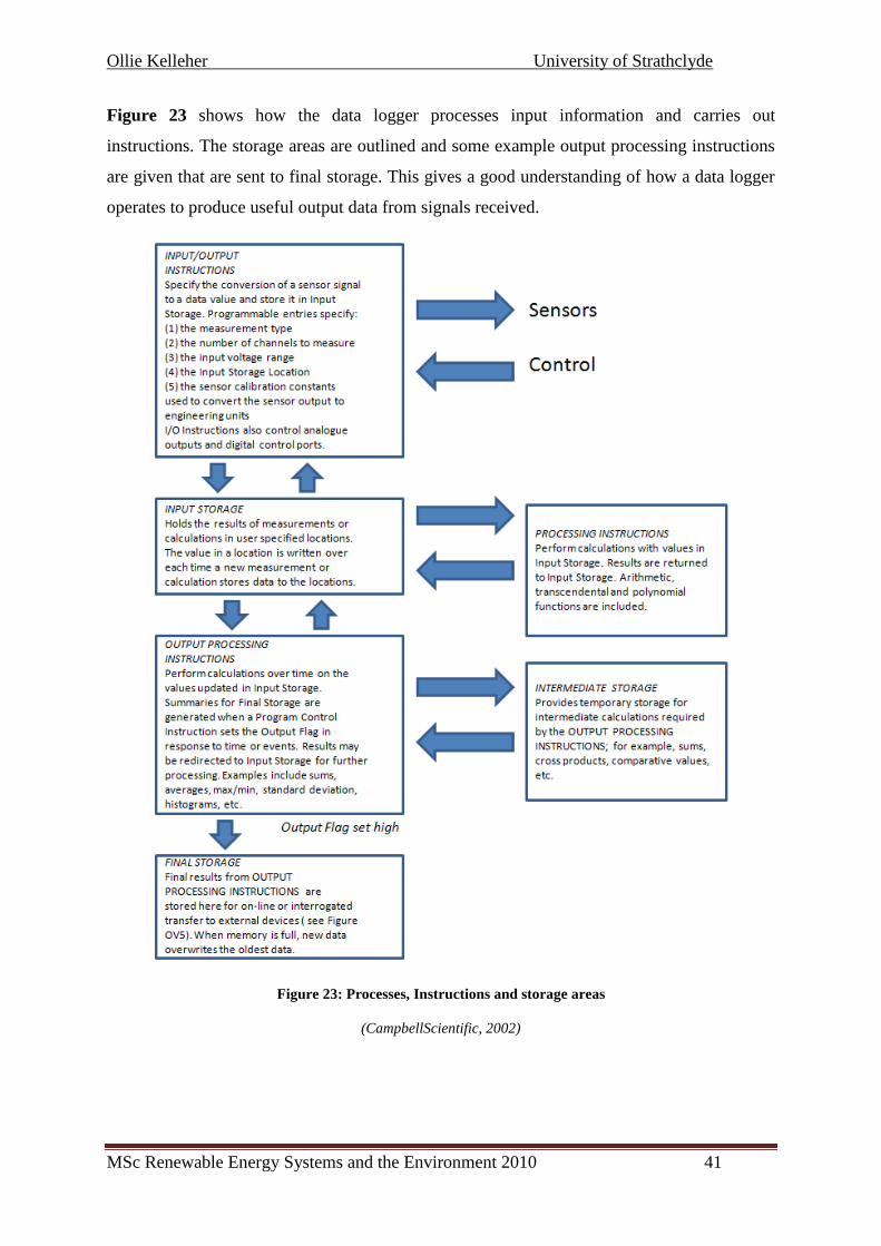
Ollie Kelleher University of Strathclyde
MSc Renewable Energy Systems and the Environment 2010 41
Figure 23 shows how the data logger processes input information and carries out
instructions. The storage areas are outlined and some example output processing instructions
are given that are sent to final storage. This gives a good understanding of how a data logger
operates to produce useful output data from signals received.
Figure 23: Processes, Instructions and storage areas
(CampbellScientific, 2002)

Ollie Kelleher University of Strathclyde
MSc Renewable Energy Systems and the Environment 2010 42
5.3.4 Remote Communication
Both the data logger and the SODAR device used in this project allow for remote
communication through the use of an external modem. The computer board that is supplied
with the SODAR comes with a serial port (COM1) that allows for connection of a GSM
modem. There is also a GSM antenna that is of significant enough length so that a sufficient
signal can be detected. The software that is used for this is SODWIN 6.0-COM. It needs to be
installed on the laptop being used to communicate with the remote modem. This software is
capable of collecting the set SODAR parameters that are currently set and it also allows for
update and altercation of new input parameters. The same software is used for
communication via a telephone modem. The modem also allows for retrieval of data obtained
by the SODAR device for analysis off site (AQSystem, 2008).
The data logger used in this project has an I/O port which can act as a 5V DC power line and
can be used to power a modem. Using a modem in conjunction with a data logger allows for
remote communication and collection of data. Retrieval of data via modem can be done under
program control or by regularly scheduled polling of the data logger. Campbell Scientific‟s
data logger support software automates this process. Telecommunications are part of the
programming command language and can be found on the prompt sheet attached in
Appendix A under instruction 97 and instruction 99. More details of this will follow in the
description of the code functionality later in section 7.5.5. The diagram in Figure 24 shows
all possible communication methods that can be used with the CR10X data logger. These
include direct connection with the device itself via a SC12 cable and then through a SC32A,
SC929 or RS232 type interface cable. These can then be connected to a laptop using an SC-
USB cable.

Ollie Kelleher University of Strathclyde
MSc Renewable Energy Systems and the Environment 2010 43
Figure 24: CR10X communication options
(CampbellScientific, 2002)
Chapter 6: Using the Data Logger
6.1 Introduction
The project was split into two separate research areas; Repair and operation of the SODAR
device on University campus, while powering it of the electricity mains, which was
conducted by my colleague Roger Carter. The other aspect, which I was dealing with, was
preparation of the mobile unit for deploying the device for operation in the field. In Chapter
5, some of the field considerations are discussed. This chapter deals more so with the
experimental work undertaken with the data logger to achieve the required goals. The two
most important apparatus that were used consist of the diesel generator and the data logger as
described in section 5.3.1 and 5.3.3 respectively, the latter which will be discussed next.

Ollie Kelleher University of Strathclyde
MSc Renewable Energy Systems and the Environment 2010 44
6.2 Initial Retrieval
The data logger was disconnected from the wiring panel initially and was located in the
trailer. The wiring panel was connected to several wires which were set to conduct various
operations that became clearer later in the project following detailed research. Initially it was
necessary to disconnect the wiring panel from all wires and remove the data logger with it
from the trailer into a lab where experimental work could be conducted on it.
The actual Campbell Scientific CR10X data logger is quite rugged and robust however some
slight damage was discovered to the D-type connection used to connect into the wiring panel.
It appeared to be bent and would not fit correctly to the wiring panel, possibly due to an
impact sustained. Luckily after the damaged pins were straightened manually using a set of
pliers, connection with the wiring panel could be re-established. Had the impact to the
connector been more severe the device may have needed to be sent to Campbell Scientific for
repair.
6.3 Powering the data logger
The data logger was powered in the laboratory by wiring it up to a 12V D.C. supply voltage.
The supply voltage was provided by the mains and converted to D.C. in a power supply unit
which allowed for adjustable voltage control. This however was fixed at 12V as required by
the data logger. Figure 25 shows the data logger in the lab with a variable D.C. voltage
supply. Note the data logger is the „can‟ shaped rugged silver metallic unit connected to the
wiring panel on the front of it on the right hand side of the photograph.
Figure 25: Data logger and supply voltage

Ollie Kelleher University of Strathclyde
MSc Renewable Energy Systems and the Environment 2010 45
6.4 Establishing Communication
6.4.1 Setting up the apparatus
The data logger came with a blue SC12 cable in the trailer (which can also be seen in Figure
25), and it was thought that by connecting this to the CS I/O port on the wiring panel and then
to a SC-USB cable before plugging it into a laptop, that it would be possible to communicate
to the logger. A number of factors needed to be considered first:
Installation of the software for the SC-USB cable and establishing which COM port
the cable operated under.
Downloading of PC200W, free software available from the Campbell Scientific
website used to program and communicate with data loggers.
Having completed all this it was still not possible to connect with the logger. A voltmeter was
used to ensure that power was running through the wiring panel by checking that there was a
voltage between the 5V supply and ground inputs available on the panel which can be used to
power a modem or other device as discussed in section 5.3.4. This was present, meaning that
the data logger was receiving power and that the internal battery was not dead. Following this
inspection, a contact was established within Campbell Scientific, Franco Casule, who was
familiar with this particular device. Having sent a number of pictures of the setup
configuration it was made clear that the SC12 cable being used could not be used to
communicate with the logger as the interface was not SC-USB Interface, but a USB to Serial
Interface. The blue SC12 cable that was originally used is just a through cable and not an
interface. For this reason it was necessary to purchase an interface which could be used to
connect into a computer or a laptop. The most inexpensive SC929 cable was chosen and
ordered for delivery.
6.4.2 Connecting to the Data Logger
Upon delivery, once everything was set up correctly, it was found that the data logger
appeared to be password protected from previous usage and would not allow connection. This
particular model allows for three levels of password security on the device and this is
explained in detail in the user manual however it is not of significant importance at this stage.
The existing code that was on the data logger would not allow connection unless the
password was entered correctly and it was not possible to override without re-setting the

Ollie Kelleher University of Strathclyde
MSc Renewable Energy Systems and the Environment 2010 46
device. As the password was not available the only solution was to re-set the logger. This was
achieved by uploading a new operating system using the device configuration utility
hardware configuration function (See Figure 26) on PC200W software. Having successfully
re-set the data logger it was then possible to conduct preliminary simulations.
6.5 Preliminary Programming
6.5.1 Software description
As mentioned previously, the software used in the initial stages of this project was PC200W.
It is designed for collecting data and is in comma-separated format ready for easy importation
into data analysis packages such as MS Excel. It can also be used for setting the data logger
clock, checking measurements and graphically displaying input locations in real-time. An
inbuilt function within PC200W is an option to create a program using an application called
Short Cut (See Figure 26). With Short Cut you can select sensors, choose output data, and
create wiring tables. The steps involved using Short Cut for building data logger programs
are as follows:
Select Scan interval (time between measurements taken),
Select sensor from a built in library,
Select measurement outputs (Max, Min, Average etc.),
Automatically generate an appropriate data logger program (in .DLD code),
Review wiring tables, data label tables and output lists.
Figure 26 shows a screen shot of PC200W and the location of some the functions described.

Ollie Kelleher University of Strathclyde
MSc Renewable Energy Systems and the Environment 2010 47
Figure 26: Screenshot of PC200W
6.5.2 Program Tests
As no external sensors were available for the data logger that matched any of those in the
inbuilt library some basic programming tests were conducted using sensors built into the
logger and some external wiring connected to the wiring panel.
Data logger Internal Temperature
The first measurement that was carried out was the internal temperature of the data logger
using a thermistor that is located inside the device on the analog board. The scan interval was
set for every 10 seconds and the output measurements included the Max, Min, Average and
Standard Deviation. The results obtained were as expected and do not require any discussion
as the experiment is only part of the familiarisation process of operating of the data logger.
The results can be found in Figure 27 and in Table 3 in section 6.5.3.

Ollie Kelleher University of Strathclyde
MSc Renewable Energy Systems and the Environment 2010 48
Data logger Battery Voltage
The next measurement that was taken and logged into the data logger‟s memory was the
voltage supplied to the device. The CR10X operates at a nominal 12V DC. Below 9.6V or
above 16V the CR10X will not operate correctly. Again the scan interval was set for every 10
seconds. Similar to before, the output measurements included Max, Min, Average and
Standard Deviation. As the power supply used to convert the mains electricity was variable it
was initially set to 12V and lowered in five intervals until the logger failed to operate. It was
not increased for fear of damaging internal components. The results displayed the decline in
voltage until the CR10X stopped working. These results can also be found in Figure 27 and
in Table 3 in section 6.5.3.
Single Ended Voltage
The final preliminary measurement that was taken with the data logger using PC200W was a
basic single ended voltage. Two wire sensors (signal and ground) were used to measure the
voltage on a single-ended channel relative to ground. The scan interval was again set for
every 10 seconds. A multiplier was used to convert the result from milliVolts to Volts. The
two wires used to make measurements were connected to the data logger into input locations
1H and AG. The other ends of the wires were connected to a simple 1.5V battery to the
positive and negative terminals. More details on wiring the data logger will be given later on
for more complex experiments. Again, the results can be found in Figure 27 and in Table 3
in section 6.5.3.

Ollie Kelleher University of Strathclyde
MSc Renewable Energy Systems and the Environment 2010 49
6.5.3 Preliminary Programming Results
As discussed, PC400W shortcut function automatically generates the DLD code necessary to
take measurements that is uploaded to the data logger. The results of the basic measurements
taken are displayed in Figure 27 and Table 3.
Figure 27: Preliminary data logger results
Table 3: Preliminary measurements logged
Average Max Min Standard Deviation
Internal Temperature 23.48 23.8 23.2 0.175119007
Supply Voltage 10.98333 12.1 9.9 0.854205284
Single ended Voltage 1.4 1.4 1.4 -
6.5.4 Discussion of Results
The results obtained were as expected. The internal temperature rose slightly with time
however it appeared to level off. The Supply voltage dipped according to the five incremental
reductions as outlined in 6.5.3. The Single ended voltage logged a voltage from a 1.5V
battery that appeared to be drained by 0.1V.

Ollie Kelleher University of Strathclyde
MSc Renewable Energy Systems and the Environment 2010 50
It is possible to retrieve the DLD code that was uploaded to the data logger for each
individual program and analyse it using the prompt sheet (see Appendix A) which is also
available from Campbell Scientific. As PC200W is limited to developing programs that are
restricted to sensors contained in the built in library that is part of Short Cut, the functionality
of the data logger is limited and does not allow it to reach both its full potential, and to
conduct the objectives required as part of this project. For this reason, more advanced
programming Campbell Scientific software was obtained on a free 30-day trial to achieve the
required results. This is known as LoggerNet 4.0.
Chapter 7: Applying the Data Logger
7.1 Introduction
As discussed in section 5.3.1 one deployment consideration for operating a SODAR device is
the availability of power. The presence of the Yanmar diesel engine synced with a Fischer
Panda generator overcomes this issue. The combined apparatus is controlled with the
presence of the CR10X data logger which is wired to monitor the performance and conduct
control operations. Before it was possible to implement the data logger to conduct the
necessary functions, the generator and diesel engine needed to be inspected and repaired
accordingly.
7.2 Engine Maintenance
7.2.1 Replacing the battery
The engine used in this project requires a 12V heavy duty battery connected in order to start
it up. The supply voltage is used to power the control panel which consists of the main on/off
switch, operation counter, generator start button, motor temperature light, oil pressure light,
operating state display, and battery charging control light. The battery also supplies power to
the fuel pump and actuator which are part of the start up process (FischerPanda). The original
battery that was removed read a voltage of around 6V. Having connected it to a charger
adjusting the input voltage and current supply, it was felt, after reviewing the readings, that a
number of cells inside the battery were more than likely exhausted. An alternative newer
battery was acquired and charged for twenty four hours until a 12V reading was detected. The
battery was then connected to the generator and the control panel light up once the switch

Ollie Kelleher University of Strathclyde
MSc Renewable Energy Systems and the Environment 2010 51
was flicked on. The generator started once the start button was pressed and the speed control
temporarily adjusted.
7.2.2 Changing the Oil
Given that the number of operational hours read 1950, and it was not clear when any
maintenance was last carried out on the diesel engine, it was considered necessary to do some
to make sure no other issues were encountered. Using the Yanmar operational manual a step
by step guide was followed to change the oil and clean the oil filter (Yanmar, 2005). First of all
the oil was drained using the connected hose at the base of the engine. Next the oil filter was
removed and cleaned thoroughly removing any dirt accumulated. Finally the two dip sticks
and oil filter were put back in place before re-sealing the hose. Clean Castrol Magnatec SAE
15W-30 oil was then put into the engine. The generator was started up and allowed to run for
5 minutes before being shut down and the oil level checked and modified accordingly.
7.2.3 Adjusting the throttle
Initially when the start button was pressed the engine would only turn over repeatedly but not
run completely until the speed control throttle was pushed temporarily. Having identified this
issue it was deemed necessary to permanently modify its position so that the engine would
start solely by hitting the start button. This was carried out using a spanner to loosen the bolt
and adjust its position before retightening it.
The diesel engine and generator were then operating smoothly and delivering a consistent
power supply. This meant that the next stage of the project required reconnecting the data
logger and programming it to conduct control operations and monitor performance.
7.3 Control and Operation Requirements
The data logger is used in conjunction with the engine and the generator. Circuitry is wired
up accordingly and will be discussed at a later stage. The presence of a GSM modem also
allows alarm messages to be sent out to inform the operator via txt message to a mobile
phone. First the control functions of the data logger will be discussed.
The data logger is implemented to retrieve, process and store data, and also perform
operations. The data collected includes:
Outside temperature (Max, Min, Average)
CR10X and Generator start up 12V battery Voltage

Ollie Kelleher University of Strathclyde
MSc Renewable Energy Systems and the Environment 2010 52
Generator Run time (Max, Min)
The Number of failed modem attempts.
Operations carried out include:
Generator operation intervals
Monitor fuel level
Monitor battery levels
Send alarm signals.
More detail of the program used to achieve this and a description of the wiring diagram
follows.
7.4 Programming Software
7.4.1 LoggerNet 4.0
LoggerNet is a more advanced version of PC200W that allowes increased logger capabilities.
The software has a very user friendly interface that is easily navigable. It enables users to set
up, configure, and retrieve data from a network of Campbell Scientific data loggers and share
this data over an Ethernet communications network. Some of the functions included allow
multiple remote monitoring and control of several separate data loggers. There are also
powerful built in data analysis tools. As well as Short Cut, (the built in function used to create
programs described in 6.5.1) there are advanced functions included that allow the
development of programs for specific needs. These are known as CR Basic Editor,
Transformer and Edlog as shown in Figure 28.
Figure 28: Logger Net user interface

Ollie Kelleher University of Strathclyde
MSc Renewable Energy Systems and the Environment 2010 53
7.4.2 Edlog
Edlog is a tool to create and edit data logger programs for all Campbell Scientific data
loggers. Instructions are available for sensor measurement, intermediate processing, program
and peripheral control, and data storage. The CR10X instruction and parameter prompt sheet
attached (Appendix A) can be used in conjunction with it to assist with inputting values
according to requirements. The built-in pre compiler provides error checking and warns of
potential problems in the program. Edlog produces a DLD file type that can be uploaded to
the logger to carry out the necessary functions. Edlog was used in conjunction with
LoggerNet to write the code necessary to perform functions and take measurements as
outlined in section 7.3.1.
7.5 Programming Description
7.5.1 Introduction
The program created is based on the original however it is modified and commented in more
detail. The program does not consider the presence of the SODAR device as in this instance it
was not ready for connection in the mobile trailer for a number of reasons. For one, the
batteries that powered it appeared to be exhausted and need to be replaced and also the circuit
was simplified to try and obtain some measurements and results. This section describes some
of the processing instructions that are taking place within the data logger that may be
dependent on input signals and measurements.
7.5.2 Digital I/O Ports
Terminals C1 to C8 on the data logger are digital input/output ports. They are generally used
for reading the status of an external signal. They are either set in a high or low state. High and
low conditions are: 3V < high < 5.5V; -0.5V < low < 0.8V. They can also be configured as
output ports and supply control (on/off) of external devices, in this case the generator and the
modem. Ports 1-5 that are used in this project are described in Table 4. The code that is
referred to is the program uploaded to the logger to carry out such functions and can be found
in Appendix B.
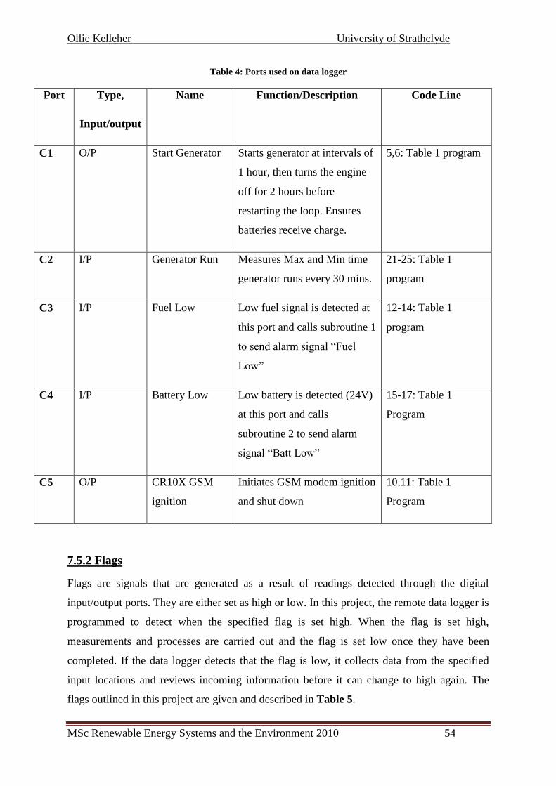
Ollie Kelleher University of Strathclyde
MSc Renewable Energy Systems and the Environment 2010 54
Table 4: Ports used on data logger
Port Type,
Input/output
Name Function/Description Code Line
C1 O/P Start Generator Starts generator at intervals of
1 hour, then turns the engine
off for 2 hours before
restarting the loop. Ensures
batteries receive charge.
5,6: Table 1 program
C2 I/P Generator Run Measures Max and Min time
generator runs every 30 mins.
21-25: Table 1
program
C3 I/P Fuel Low Low fuel signal is detected at
this port and calls subroutine 1
to send alarm signal “Fuel
Low”
12-14: Table 1
program
C4 I/P Battery Low Low battery is detected (24V)
at this port and calls
subroutine 2 to send alarm
signal “Batt Low”
15-17: Table 1
Program
C5 O/P CR10X GSM
ignition
Initiates GSM modem ignition
and shut down
10,11: Table 1
Program
7.5.2 Flags
Flags are signals that are generated as a result of readings detected through the digital
input/output ports. They are either set as high or low. In this project, the remote data logger is
programmed to detect when the specified flag is set high. When the flag is set high,
measurements and processes are carried out and the flag is set low once they have been
completed. If the data logger detects that the flag is low, it collects data from the specified
input locations and reviews incoming information before it can change to high again. The
flags outlined in this project are given and described in Table 5.

Ollie Kelleher University of Strathclyde
MSc Renewable Energy Systems and the Environment 2010 55
Table 5: Flag description
Flag Name Function Code Line
F1-Low Fuel Re-set modem if high disabling
communication for sub-routine 1
2,3,12 : Table 3 subroutine 1
F2-Low Battery
(24V)
Re-set modem if high disabling
communication for sub-routine 2
16,17,26 : Table 3 subroutine 2
F3-Low Battery
CR10X
Re-set modem if high disabling
communication for sub-routine 3
30,31,40 : Table 3 subroutine 3
F5-Re-dial Low Fuel Allows for subroutine 1 to be
called and communication
initiated if high. Impacted by C3
2,13: Table 1
13: Table 3 Subroutine 1
F6-Re-dial Low
Batt(24V)
Allows for subroutine 2 to be
called and communication
initiated if high. Impacted by C4
3,16: Table 1
27: Table 3 Subroutine 2
F7-Re-dial Low Batt
(CR10X)
Allows for subroutine 3 to be
called and communication
initiated if high. Impacted by
measured voltage <12V
4,19: Table 1
41: Table 3 Subroutine 3
Flags 1-3 have a default setting of low until after communication has been carried out to
prevent the modem from contacting the mobile phone in succession. The modem is limited to
two calls every twenty four hours. Flags 5-7 are initially set high to allow subroutines to be
called and communication alarms if necessary. However, they are set low once the
corresponding subroutine has run again to prevent constant re-dial.

Ollie Kelleher University of Strathclyde
MSc Renewable Energy Systems and the Environment 2010 56
7.5.3 Run Generator
The program signals to run the generator at intervals of one hour on and two hours off. This
makes sure the batteries receive adequate charge consistently. Also If C2 is set high the
generator detects an input signal in the form of Z which also signals the generator to operate.
See code lines 5,6,20,21 (Appendix B).
7.5.4 Output processing
The data is collected in the storage module of the memory every thirty minutes. The array ID
is 501 and the time is logged with the information gathered. Although readings are taken
every ten seconds, it is the processed result of that data that is stored. The data included in the
output array is listed in Table 6, a screenshot of the final storage information collected taken
from Edlog.
Table 6:Final Storage data

Ollie Kelleher University of Strathclyde
MSc Renewable Energy Systems and the Environment 2010 57
7.5.5 Subroutines
Subroutine 1, 2, and 3 are almost identical except for the fact that they all deliver different
messages. The Alarm message delivered by each subroutine is as follows:
Subroutine 1: ALARM! FUEL LOW
Subroutine 2: ALARM! BATT LOW
Subroutine 3: ALARM! CR10 LOW
The subroutine begins by initiating communication with the GSM using instruction 97. The
type of modem selected is generic with a 9600 baud rate. The model used is a Wavecom
Fastrack supreme. The call time limit is set to 20 seconds and fast retry is set to 60 seconds in
the case of a failed attempt. The number of failed attempts is stored in the data logger‟s
memory. Communication is conducted with the modem through the use of American
Standard Code for Information Interchange (ASCII), which is listed in Appendix E of the
user manual for the CR10X data logger. Initial commands are sent to the modem prior to
dialling out the required number. Once a response has been detected the modem then
proceeds to sending a message which is different for each subroutine in this case as outlined.
Further commands are conducted before communication is ceased and retried if unsuccessful,
otherwise is successful, the flag 1 is set high to reset the modem and flag 5 is set low to
prevent unnecessary redial.

Ollie Kelleher University of Strathclyde
MSc Renewable Energy Systems and the Environment 2010 58
7.6 Wiring the data logger
The circuit diagram of the wiring diagram used to connect the data logger to all necessary
devices used in this project and described in the code is given in Appendix C. The input port
for each wire and a description of the colour used is given in this drawing. A complete
comprehension of the circuitry used was required to understand where all input and output
signals are coming from. At each input location there is a note on the signal being received.
Displayed is:
CR10X wiring panel with connected wires,
Fuel gauge with corresponding relays
Fuse connections for 12V and 24V supplies.
Temperature Probe
12V logger battery
GSM Modem
SC12 and SC929 cables
Laptop Computer
The wiring diagram is modified from the original one given as some of the apparent wiring
outlined did not seem to be present although it was felt that there was enough to connect
everything sufficiently to run the program that was created and uploaded to the data logger.

Ollie Kelleher University of Strathclyde
MSc Renewable Energy Systems and the Environment 2010 59
Chapter 8: Results and Discussion
8.1 Introduction
This chapter reflects on the work conducted and achievements obtained throughout this
project. The experimental procedures undertaken have contributed to significant learning in
the understanding and operation of the devices used.
8.2 Laboratory experiments
A significant amount of time was spent understanding the theoretical operation and control
capabilities surrounding the use of the data logger by studying the operation manual. Once
connected and functional in the laboratory, basic measurements were taken, having
established a form of connection, and acquired the software to do so. These results have
already been identified and are discussed in section 6.5. The procedure of initial data logger
use is well documented throughout Chapter 6.
The outcome of the laboratory experiments showed that the logger was functioning as
expected producing predicted results. Also increased familiarity with the software and
programming techniques led to the acquisition of a more advanced program compiler.
8.3 Generator Repair
Prior to applying the logger for practical use and achieving the targeted control and operation
requirements it was first necessary to identify and conduct repair to the engine and generator.
Initially it was thought that the device was a standalone generator supplied by Fischer Panda.
Upon further investigation it was discovered that a Yanmar diesel engine was synced in with
the generator and operating via a control panel supplied with the generator. Some time was
spent establishing the type of engine used to drive the generator and an operation manual was
acquired to conduct service as necessary. The battery was also replaced to provide an
electrical start capability to the control panel. All of the work described was clearly outlined
in section 7.2 and carried out successfully.

Ollie Kelleher University of Strathclyde
MSc Renewable Energy Systems and the Environment 2010 60
The result of the work carried out led to increased familiarity with the combined engine-
generator operation. It also meant that power was now available in the mobile trailer unit
should any field testing of the SODAR be carried out in the future.
8.4 Data Logger Application
8.4.1 Achieved Goals
Having gained a complete understanding of operation, and applied the data logger
experimentally the next stage was to apply it for use in the required scenario. The
functionality goal of the data logger for use in this project has been clearly described in
section 7.3. The process in achieving that goal is also described in detail and the steps
undertaken to manipulate and develop instructions in Edlog are also well documented
throughout section 7.5.
The result of this part of the project included:
Successful development of the program to achieve necessary results
Uploading the program to the data logger
Understanding of necessary wiring to apply logger functionality
Established direct communication and monitoring of data, flag and port status
Sent out Alarm message via the GSM modem having detected low battery on the
batteries used to supply the SODAR device.
All of these aspects were successful and described with the information used, modified and
given in Appendix A, B&C. Some problems were encountered along the way however,
which impacted the collection of useful data.

Ollie Kelleher University of Strathclyde
MSc Renewable Energy Systems and the Environment 2010 61
8.4.2 Identified issues
Upon wiring the data logger accordingly to run on the uploaded program some issues were
encountered. First of all the black and grey wires connected to the green plug used to supply
power to the data logger through the wiring panel seemed to be delivering a very low voltage
that was not significant enough to power it up. This was overcome by directly connecting the
data logger to the 12V battery used for the generator start up.
Upon inserting all other necessary input wires, obtaining a power source and starting the
generator, further issues were encountered. The readings that were being detected by the
logger in the connect function of LoggerNet, upon direct connection through the use of an
SC929 cable via an SC-USB to a laptop, appeared to be of no use and significantly
inaccurate. Having successfully compiled the program and reviewed it thoroughly the
suspected reason was believed to be in the mobile trailers circuitry. The data logger was
shown to log information however it was not as predicted. This was assumed to be due to
incorrect input signals being obtained. This proved to be quite disappointing and the
remainder of the project focused upon checking the wiring of the trailer and making sure all
fuses were functional and that signals were being sent and received accordingly. Efforts made
were of no avail and therefore no data was successfully collected for report in this part of the
project due to potential circuitry malfunction which could not be identified in time.

Ollie Kelleher University of Strathclyde
MSc Renewable Energy Systems and the Environment 2010 62
Chapter 9: Conclusion and Recommendations
9.1 Conclusions
Overall, this project focused on a very broad spectrum and global scale before being
narrowed down to a specific aspect that contributes to its entirety. To recap on the
development of issues and the structured process taken within this project the key areas and
their relationship are as follows:
Global environmental and economical issues,
Identified solution in the form of wind,
Wind energy history, market potential and possible constraints,
Wind measurement techniques,
SODAR and the technology,
Applying SODAR in the field,
Control aspects of a diesel generator used to power a SODAR device,
Using a Campbell scientific data logger to achieve control and operational goals.
By reviewing such a wide variety of information, significant learning‟s were achieved and
more specifically the outlined goal of the project title was achieved successfully in the form
of theoretical application. Practical application was also achieved in the form of; successfully
understanding how the data loggers operates, obtaining preliminary laboratory test results,
successful repair of the generator used, modifying and developing the coding and instructions
used to program the data logger, uploading the program and communicating with the data
logger while connected to the circuitry described in Appendix C.
More complete practical application would see a return of useful data from the data logger
and fully functional circuitry of the mobile trailer unit. However, unfortunately due to the
time constraint that limited this project duration a solution could not be established that
would produce the output data required prior to report submission. It was felt however, if
further analysis of the circuitry could be conducted that the data logger was sufficiently
programmed to produce the outlined output results and conduct the identified control
operations, provided the input signals were valid.

Ollie Kelleher University of Strathclyde
MSc Renewable Energy Systems and the Environment 2010 63
Although it is believed that the program uploaded is comprehensive and fully functional if
wired correctly, perhaps it proved to be a step too far as it is quite advanced coding. An
alternative approach would have been to simulate the intended results in the laboratory
through individual programs designed to produce an output for that particular parameter or
control operation. This was overlooked due to the lack of practical application having
successfully got the generator operational. It may however, be necessary to do in order to
comprehend reasons for identified issues with circuitry in the future.

Ollie Kelleher University of Strathclyde
MSc Renewable Energy Systems and the Environment 2010 64
9.2 Recommendations
The most important aspect that needs to be conducted to achieve a fully functional mobile
trailer unit for the SODAR is to validate all existing circuitry. This would prove to be quite a
significant task and was outside the scope of this project due to time constraints. If all
circuitry is fully functional it would mean that the uploaded program could operate as
required and produce valid results.
Also, as the SODAR is being used to measure wind data and potentially identify sites for a
wind turbine, it would seem logical to look at potential renewable sources of power to keep in
conjunction with overall sustainability. Such options could include Photo Voltaic Solar
Panels that could be used to charge the batteries particularly in climates that may be suitable
or during summer months.
If all circuitry was validated and the logger adequately operating in conjunction with the
GSM modem, the given code could be modified to include the presence of the SODAR
device, and the potential for a field test would exist. If this could be achieved, it would be
possible to conduct accurate calibration and comparison of results with other remote wind
measuring devices and cup anemometers at the test site discussed in section 4.1. This test site
is fully commissioned and located in Worcestershire where they have a 90m met mast with
an anemometer attached installed. This location would prove ideal to correlate results
obtained from the SODAR, anemometer and potentially any LIDAR devices present if the
data was made available. The results obtained at this remote location may prove to be more
accurate than those from a rooftop in an urban canopy where the device currently lies on
campus. This site in Worcestershire is fully accessible and open for use by any interested
parties.
Identifying the necessary software, analysing the data logger operating methods, explaining
the programming application and finally, conducting maintenance on the generator, has
resulted in a solid basis for further advancement in achieving a fully functional mobile trailer
unit for the SODAR device. All of these achievements discussed throughout the project will
greatly assist in the deployment potential for the SODAR and allow for analysis of wind
energy at multiple locations.

Ollie Kelleher University of Strathclyde
MSc Renewable Energy Systems and the Environment 2010 65
References
AQSystem. (2008, August 19). Wind Finder AQ500. Stcokholm, Mediavägen, Sweeden.
ART. (2008, May 24th). Atmospheric Research & Technology LLC. Retrieved June 18th,
2010, from About Sodar: http://www.sodar.com/about_sodar.htm
Bruns, E. (2002, 24 9). Environmental issues of offshore wind farms. Retrieved 11 25, 2009,
from IEA WIND:
http://www.ieawind.org/Task_11/TopicalExpert/Summary_40_Offshore.pdf
Buck, S. a. (2008, 11 14). Forest Encycleopedia Network. Retrieved July 28th, 2010, from
Mechanical and Thermal Turbulence:
http://www.forestencyclopedia.net/p/p418/i/i32/view?showNav=n
BWEA. (2009). Wind Energy in the UK, State of the Industry Report. London: British Wind
Energy Association.
C.B. Hasager, P. A. (2007, April). Riso National Laboratory. Retrieved August 7, 2010, from
Technical University of Denmark: http://130.226.56.153/rispubl/reports/ris-r-1586.pdf
CampbellScientific. (2002). CR10X Measurement and control module instruction manual.
Retrieved June 5, 2010, from Campbell Scientific Europe: http://www.campbellsci.co.uk/
Daily, S. (2010, August 3). Science News. Retrieved August 13, 2010, from New Carbon
dioxide Emmissions Model:
http://www.sciencedaily.com/releases/2010/08/100802110827.htm
EAI. (2010, July 10). Internation Energy Outlook 2010. Retrieved July 15, 2010, from U.S.
Energy Information Administration: http://www.eia.doe.gov/oiaf/ieo/pdf/highlights.pdf
ECORATER. (2010). Wind Power Energy. Retrieved July 5, 2010, from copyright ETSU for
DTI 1999: http://www.ecorater.co.uk/wind-power-energy.shtml
EWEA. (2010). Wind Energy The Facts. Retrieved July 10, 2010, from http://www.wind-
energy-the-facts.org/en/part-i-technology/chapter-3-wind-turbine-technology/evolution-of-
commercial-wind-turbine-technology/growth-of-wind-turbine-size.html
FischerPanda. (n.d.). Fischer Panda Generator. Retrieved June 12, 2010, from ATG 4000
DC Generator Operation Manual: http://fischerpanda.com/Manuals/Panda%20AGT-
DC%204000%20(12V)%20Operation%20Manual.pdf
Gentry, B. (1999). Atmospheric Remote Sensing Laboratory. Retrieved July 10, 2010, from
Wind Lidar: www.ece.arizona.edu/~arsl/presentation2.ppt
Government, H. (2007). Meeting The Energy Challenge. Norwich: TSO.

Ollie Kelleher University of Strathclyde
MSc Renewable Energy Systems and the Environment 2010 66
InternationalEnergyAgency. (2007). 51st IEA Topical Expert Meeting, State of the art of
Remote Wind Speed Sensing Techniques using Sodar, Lidar and Satellites. Risø (p. 32).
Roskilde, Denmark: Sven-Erik Thor.
Ioannis Antoniou, H. E. (2003). On the Theory of SODAR Measurement Techniques.
Roskilde: RISO National Laboratory.
MacKay, D. J. (2008). Sustainable Energy - without the hot air. Cambridge.
NaturalPower. (2010, August 10). Natural Power News. Retrieved August 12th, 2010, from
http://www.naturalpower.com/news/lidar-sodar-test-site
Oldbaum. (2010, June 22). Oldbaum Services. Retrieved June 28, 2010, from
http://www.oldbaumservices.co.uk/AQ500.pdf
Peinke, J. (2007). Wind Energy. Oldenburg: Springer.
Remtech. (2009, 12). Phased Array Sodar Family for all Ranges and Applications. Retrieved
July 18, 2010, from http://www.remtechinc.com/sodar.htm
RenewableEnergyWorld. (2008, March 27). Using LIDAR for Identification of Wind
Parameters. Retrieved July 16, 2010, from Renewable Energy World:
http://www.renewableenergyworld.com/rea/news/article/2008/03/using-lidar-for-
identification-of-wind-parameters-51911
SCINTEC. (2004, January). Acoustic Wind Profilers. Retrieved August 8, 2010, from
Advanced High Performance Sodars for Wind and Turbulence:
http://www.scintec.com/PDFs/Product_Information_FAS_2007.pdf
TelosNet. (2001). Illustrated History of Wind Power Development. Retrieved July 19, 2010,
from TelosNet Web Development and Darrell Dodge:
http://www.telosnet.com/wind/early.html
Yanmar. (2005). Yanmar Italy. Retrieved August 19, 2010, from LV Series Engine:
http://www.yanmaritaly.it/pdf/manuali_operativi/LV%20OperationManual.pdf

Ollie Kelleher University of Strathclyde
MSc Renewable Energy Systems and the Environment 2010 67
Appendix A: Prompt Sheet

Ollie Kelleher University of Strathclyde
MSc Renewable Energy Systems and the Environment 2010 68

Ollie Kelleher University of Strathclyde
MSc Renewable Energy Systems and the Environment 2010 69

Ollie Kelleher University of Strathclyde
MSc Renewable Energy Systems and the Environment 2010 70
Appendix B: Program Code
Data logger Code Used to monitor and control Generator
;Data logger ports:
;C1 – O/P – Start Generator
;C2 – I/P – Generator Run
;C3 – I/P – Fuel Low
;C4 – I/P – Battery Low
;C5 – O/P – CR10X GSM ignition
;
;Scan rate 60 seconds
;averaging period – 30 minutes
;Temp – E1, SE1
;sms calls - +447581092131
;
;Flags used to initiate communication:
;F1 – P97 comms mode reset – Low fuel
;F2 – P97 comms mode reset – Low battery – 24V
;F3 – P97 comms mode reset – Low battery – CR10X
;F5 – re-dial flag – Low fuel
;F6 – re-dial flag – Low batt – 24V system
;F7 – re-dial flag – Low battery on CR10X
; - set to ensure no more than two calls to each phone every 24 hours.
;Measurement taken every 10 seconds
*Table 1 Program
01:10 Execution Interval (seconds)
;Measure External Temperature

Ollie Kelleher University of Strathclyde
MSc Renewable Energy Systems and the Environment 2010 71
1: Temp (107) (P11)
1: 1 Reps
2: 1 SE Channel
3: 1 Excite all reps w/E1
4: 1 Loc [ Temp]
5: 1.0 Mult
6: 0.0 Offset
;Set re-dial flags 5,6 and 7 high
2: If time is (P92)
1: 0 Minutes (Seconds --) into a
2: 720 Interval (same units as above)
3: 15 Set Flag 5 High
3: If time is (P92)
1: 0 Minutes (Seconds --) into a
2: 720 Interval (same units as above)
3: 16 Set Flag 6 High
4: If time is (P92)
1: 0 Minutes (Seconds --) into a
2: 720 Interval (same units as above)
3: 17 Set Flag 7 High
;Charge batteries for 1 hour then wait 2 until next charge unless flagged
;Start Generator
;5: It time is (P92)
; 1: 0 Minutes (Seconds --) into a
; 2: 120 Interval (same units as above)
; 3: 41 Set Port 1 High

Ollie Kelleher University of Strathclyde
MSc Renewable Energy Systems and the Environment 2010 72
; Stop Generator
;6: If time is (p92)
; 1: 60 Minutes (Seconds --) into a
; 2: 120 Interval (same units as above)
; 3: 51 Set Port 1 Low
;Define initial Port settings
7: Set Port(s) (P20)
1: 0007 C8..C5=low/low/low/output
2: 8887 C4..C1=input/input/input/output
;Reset CR10X data logger GSM communication (1min reset)
8: If time is (P92)
1: 5 Minutes (Seconds --) into a
2: 60 Interval (same units as above)
3: 45 Set Port 5 High
;Turn modem off provided communications with GSM have ended
9: If time is (P92)
1: 0 Minutes (Seconds --) into a
2: 60 Interval (same units as above)
3: 55 Set Port 5 Low
;Check port and flag status and calls subroutines if high
;If low fuel is detected port 3 is high and therefore sets flag 5 high and calls
subroutine 1 if necessary
10: If Flag/Port (P91)
1: 43 Do if Port 3 is High
2: 30 Then Do
11: If Flag/Port (P91)
1: 15 Do if Flag 5 is High
2: 01 Call Subroutine 1
12: End (P95)

Ollie Kelleher University of Strathclyde
MSc Renewable Energy Systems and the Environment 2010 73
;If low battery is detected (24V) port 4 is high and therefore sets flag 6 high and calls
subroutine 2 if necessary
13: If Flag/Port (P91)
1: 44 Do if Port 4 is High
2: 30 Then Do
14: If Flag/Port (P91)
1: 16 Do if Flag 6 is High
2: 02 Call Subroutine 2
15: End (P95)
;Battery measurement taken and data logger low batt flag setting calls subroutine 3 if
CR10X battery is low
16: If (XF) (P89)
1: 3 x Loc [ battery]
2: 4 <
3: 12 F
4: 30 Then Do
17: If Flag/Port (P91)
1: 17 Do if Flag 7 is High
2: 03 Call Subroutine 3
18: End (P95)
;Runs generator if input signal detected in the form of F
19: If Flag/Port (P91)
1: 42 Do if Port 2 is High
2: 30 Then Do
20: Z=F (P30)
1: 1 F
2: 0 Exponent of 10

Ollie Kelleher University of Strathclyde
MSc Renewable Energy Systems and the Environment 2010 74
3: 2 Z Loc [genrun ]
21: Else (P94)
22: Z=F (P30)
1: 0 F
2: 0 Exponent of 10
3: 2 Z Loc [genrun ]
23: End (P95)
;Measures battery voltage
24: Batt Voltage (P10)
1: 3 Loc [battery]
;Output processing of data and measurements
;Output storage format
25: Serial Out (P96)
1: 71 Storage Module
;Stores data every 30 minutes
26: If time is (P92)
1: 0 Minutes (Seconds --) into a
2: 30 Interval (same units as above)
3: 10 Set Output Flag High
;Final storage area selected
27: Set Active Storage Area (P80)^16581
1: 01 Final Storage Area 1
2: 501 Array ID
;Storage time
28: Real Time (P77)^3722
1: 1110 Year,Day,Hour/Minute
;Battery Sample Stored

Ollie Kelleher University of Strathclyde
MSc Renewable Energy Systems and the Environment 2010 75
29: Sample (P70)^1706
1: 1 Reps
2: 3 Loc [battery]
;Temperature Average, Min, Max calculated and Stored
30: Average (P71)^16989
1: 1 Reps
2: 1 Loc [ Temp ]
31: Minimum (P74)^24806
1: 1 Reps
2: 00 Time Option
3: 1 Loc [ Temp ]
32: Maximum (P73)^19768
1: 1 Reps
2: 00 Time Option
3: 1 Loc [ Temp ]
;Max & Min Generator running time Stored
33: Maximum (P73)^27526
1: 1 Reps
2: 00 Value with Hr-Min
3: 2 Loc [ genrun ]
34: Minimum (P74)^3123
1: 1 Reps
2: 10 Value with Hr-Min
3: 2 Loc [genrun ]
*Table 2 Program
02: 0.0000 Execution Interval (seconds)
;Subroutine 1,2, and 3. Communication with Modem.

Ollie Kelleher University of Strathclyde
MSc Renewable Energy Systems and the Environment 2010 76
;Subroutine 1, Low fuel message
*Table 3 Subroutines
1: Beginning of Subroutine (P85)
1: 01 Subroutine 1
2: Do (P86)
1:21 Set Flag 1 Low
;Call back command is run once flag 1 is reset
3: Initiate Telecommunications (P97)
1: 72 Generic Modem/9600 Baud; Use the Generic modem to send the
string
2: 1 Disabled when User Flag 1 is High
3: 20 Seconds Call Time Limit ; Should be long enough with a 10 sec
timeout
4: 60 Seconds Before Fast Retry ; just in case it fails
5: 2 Fast Retries
6: 60 Minutes before Slow Retry
7: 4 Failures Loc [number_fail_connection
8: 0000 Call-back ID
;Number dialled +447581092131. ACII binary digital characters used to transfer data.
Initially communication is established with modem commands made.
4: Extended Parameters 4 digit (P68)
1: 87 Option
2: 100 Option
3: 69 Option
4: 24 Option
5: 65 Option
6: 84 Option
7: 43 Option
8: 67 Option
;Number entered

Ollie Kelleher University of Strathclyde
MSc Renewable Energy Systems and the Environment 2010 77
5: Extended Parameters 4 digit (P68)
1: 77 Option ;M
2: 71 Option ;G
3: 83 Option ;S
4: 61 Option ;=
5: 34 Option ;”
6: 43 Option ;+ it is best to enter the number in international format
7: 52 Option ;4
8: 52 Option ;4
6: Extended Parameters 4 digit (P68)
1: 55 Option ;7
2: 53 Option ;5
3: 56 Option ;8
4: 49 Option ;1
5: 48 Option ;0
6: 57 Option ;9
7: 50 Option ;2
8: 49 Option ;1
7: Extended Parameters 4 digit (P68)
1: 51 Option ;3
2: 49 Option ;1
3: 34 Option ;”
4: 13 Option ;Terminate with carriage return, then wait for response
5: 82 Option ; R – Rx chars – this waits for the “LF > Space”
6: 3 Option ; 3 chars
7: 10 Option ;LF
8: 62 Option ;>;
;Message sent once connection established : “ALARM! Fuel Low”

Ollie Kelleher University of Strathclyde
MSc Renewable Energy Systems and the Environment 2010 78
8: Extended Parameters 4 digit (P68)
1: 32 Option ; space
2: 69 Option ;E – Tx with echo, now send the message
3: 15 Option ; 15 chars
4: 65 Option ;A
5: 76 Option ;L
6: 65 Option ;A
7: 82 Option ;R
8: 77 Option ;M
9: Extended Parameters 4 digit (P68)
1: 33 Option ;!
2: 32 Option ;
3: 70 Option ;F
4: 85 Option ;U
5: 69 Option ;E
6: 76 Option ;L
7: 32 Option ;
8: 76 Option ;L
10: Extended Parameters 4 digit (P68)
1: 79 Option ;O
2: 87 Option ;W
3: 84 Option
4: 1 Option
5: 26 Option
6: 87 Option
7: 100 Option
8: 82 Option
11: Extended Parameters 4 digit (P68)

Ollie Kelleher University of Strathclyde
MSc Renewable Energy Systems and the Environment 2010 79
1: 3 Option
2: 10 Option
3: 48 Option
4: 13 Option
5: 000 Option
6: 0000 Option
7: 0000 Option
8: 0000 Option
12: Do (P86)
1: 11 Set Flag 1 High
13: Do (P86)
1: 25 Set Flag 5 Low
14: End (P95)
;Subroutine 2, Battery Low on 24V System message
15: Beginning of Subroutine (P85)
1: 02 Subroutine 2
16: Do (P86)
1: 22 Set Flag 2 Low
;Call back command is run provided flag 2 is reset
17: Initiate Telecommunications (P97)
1: 72 Generic Modem/9600 Baud ; Use the Generic modem to send the
string
2: 2 Disabled when User Fag 2 is High
3: 20 Seconds Call Time Limit ; Should be long enough with a 10 sec
timeout
4: 60 Seconds Before Fast Tetry ; just in case it fails
5: 2 Fast Retries
6: 60 Minutes before Slow Retry
7: 4 Failures Loc [no_fails

Ollie Kelleher University of Strathclyde
MSc Renewable Energy Systems and the Environment 2010 80
8: 0000 Call-back ID
;Number dialled +447581092131. ACII binary digital characters used to transfer data.
Initially communication is established with modem commands made.
18: Extended Parameters 4 digit (P68)
1: 87 Option
2: 100 Option
3: 69 Option
4: 24 Option
5: 65 Option
6: 84 Option
7: 43 Option
8: 67 Option
;Number entered
19: Extended Parameters 4 digit (P68)
1: 77 Option ;M
2: 71 Option ;G
3: 83 Option ;S
4: 61 Option ;=
5: 34 Option ;”
6: 43 Option ;+ international format
7: 52 Option ;4
8: 52 Option ;4
20: Extended Parameters 4 digit (P68)
1: 55 Option ;7
2: 53 Option ;5
3: 56 Option ;8
4: 49 Option ;1
5: 48 Option ;0
6: 57 Option ;9

Ollie Kelleher University of Strathclyde
MSc Renewable Energy Systems and the Environment 2010 81
7: 50 Option ;2
8: 49 Option ;1
21: Extended Parameters 4 digit (P68)
1: 51 Option ;3
2: 49 Option ;1
3: 34 Option;”
4: 13 Option; Terminate with carriage return, then wait for response
5: 82 Option ; R – Rx chars – this waits for the “LF > SPACE” response
6: 3 Option ; 3 chars
7: 10 Option ; LF
8: 62 Option ; >;
;Message sent once connection established : “ALARM! BATT LOW”
22: Extended Parameters 4 digit (P68)
1: 32 Option ; space
2: 69 Option; E – Tx with echo, now send the message
3: 15 Option; 15 chars
4: 65 Option; A
5: 76 Option ; L
6: 65 Option ;A
7: 82 Option ;R
8: 77 Option ;M
23: Extended Parameters 4 digit (P68)
1: 33 Option ;!
2: 32 Option;
3: 66 Option; B
4: 65 Option; A
5: 84 Option ; T
6: 84 Option ; T

Ollie Kelleher University of Strathclyde
MSc Renewable Energy Systems and the Environment 2010 82
7: 32 Option ;
8: 76 Option ; L
24: Extended Parameters 4 digit (P68)
1: 79 Option ;O
2: 87 Option; W
3: 84 Option
4: 1 Option
5: 26 Option
6: 87 Option
7: 100 Option
8: 82 Option
25: Extended Parameters 4 digit (P68)
1: 3 Option
2: 10 Option
3: 48 Option
4: 13 Option
5: 000 Option
6: 0000 Option
7: 0000 Option
8: 0000 Option
26: Do (P86)
1: 12 Set Flag 2 High
27: Do (P86)
1: 26 Set Flag 6 Low
28: End (P95)
;Subroutine 3, CR10X Data logger Battery Low message
29: Beginning of Subroutine (P85)
1: 03 Subroutine 3

Ollie Kelleher University of Strathclyde
MSc Renewable Energy Systems and the Environment 2010 83
30: Do (P86)
1: 23 Set Flag 3 Low
;Call back command is run provided flag 3 is reset
31: Initiate Telecommunications (P97)
1: 72 Generic Modem/9600 Baud ; Should be long enough to send the
string
2: 3 Disabled when User Flag 3 is High
3: 20 Seconds Call Time Limit ; Should be long enough with a 10 sec
timeout
4: 60 Seconds Before Fast Retry ; just in case it fails
5: 2 Fast Retries
6: 60 Minutes before Slow Retry
7: 4 Failures Loc [no_fails
8: 0000 Call-back ID
;Number dialled +447581092131. ACII binary digital characters used to transfer data.
Initially communication is established with modem commands made.
32: Extended Parameters 4 digit (P68)
1: 87 Option
2: 100 -- Option
3: 69 Option
4: 24 Option
5: 65 Option
6: 84 Option
7: 43 Option
8: 67 Option
;Number entered
33: Extended Parameters 4 digit (P68)
1: 77 Option ;M
2: 71 Option ;G
3: 83 Option ;S

Ollie Kelleher University of Strathclyde
MSc Renewable Energy Systems and the Environment 2010 84
4: 61 Option ;=
5: 34 Option ;”
6: 43 Option ;+ it is best to enter the number in international format
7: 52 Option ;4
8: 52 Option ;4
34: Extended Parameters 4 digit (P68)
1: 55 Option ;7
2: 53 Option ;5
3: 56 Option ;8
4: 49 Option ;1
5: 48 Option ;0
6: 57 Option ;9
7: 50 Option ;2
8: 49 Option ;1
35: Extended Parameters 4 digit (P68)
1: 51 Option ;3
2: 49 Option ;1
3: 34 Option ;”
4: 13 Option ;Terminate with carriage return, then wait for response
5: 82 Option ; R – Rx chars – this waits for the “LF > SPACE” response
6: 3 Option; 3 chars
7: 10 Option ;LF
8: 62 Option ;>;
;Message sent once connection established : “ALARM! CR10 LOW”
36: Extended Parameters 4 digit (P68)
1: 32 Option ;space
2: 69 Option ;E – Tx with echo, now send the message
3: 15 Option ;15 chars

Ollie Kelleher University of Strathclyde
MSc Renewable Energy Systems and the Environment 2010 85
4: 65 Option ;A
5: 76 Option ;L
6: 65 Option ;A
7: 82 Option ;R
8: 77 Option ;M
37: Extended Parameters 4 digit (P68)
1: 33 Option ;!
2: 32 Option ;
3: 67 Option ;C
4: 82 Option ;R
5: 49 Option ;1
6: 48 Option ;0
7: 32 Option ;
8: 76 Option ;L
38: Extended Parameters 4 digit (P68)
1: 79 Option ;O
2: 87 Option ;W
3: 84 Option
4: 1 Option
5: 26 Option
6: 87 Option
7: 100 Option
8: 82 Option
39: Extended Parameters 4 digit (P68)
1: 3 Option
2: 10 Option
3: 48 Option
4: 13 Option

Ollie Kelleher University of Strathclyde
MSc Renewable Energy Systems and the Environment 2010 86
5: 000 Option
6: 0000 Option
7: 0000 Option
8: 0000 Option
40: Do (P86)
1: 13 Set Flag 3 High
41: Do (P86)
1: 27 Set Flag 7 Low
42: End (P95)
End Program
;Storage data input locations
1 Temp 1 3 0
2 genrun 1 2 2
3 battery 1 2 1
4 no_fails 1 0 4
6 __________ 0 0 0
7 __________ 0 0 0
8 __________ 0 0 0
9 __________ 0 0 0
10 __________ 0 0 0
11 __________ 0 0 0
12 __________ 0 0 0
13 __________ 0 0 0
14 __________ 0 0 0
15 __________ 0 0 0
16 __________ 0 0 0
17 __________ 0 0 0

Ollie Kelleher University of Strathclyde
MSc Renewable Energy Systems and the Environment 2010 87
18 __________ 0 0 0
19 __________ 0 0 0
20 __________ 0 0 0
21 __________ 0 0 0
22 __________ 0 0 0
23 __________ 0 0 0
24 __________ 0 0 0
25 __________ 0 0 0
26 __________ 0 0 0
27 __________ 0 0 0
28 __________ 0 0 0
Final Storage Labels, Output processed data
0,Year_RTM,
0,Day_RTM
0,Hour_Minute_RTM
1,battery
2, Temp_AVG
3,Temp_MIN
4,Temp_MAX
5,genrun_MAX
5,genrun_Hr_Min_MAX
6,genrun_MIN
6,genrun_Hr_Min_MIN

Ollie Kelleher University of Strathclyde
MSc Renewable Energy Systems and the Environment 2010 88
Appendix C: Wiring Diagram