Dynamical Systemsand Space Mission Design

Jerrold Marsden, Wang Koon and Martin Lo

Wang Sang KoonControl and Dynamical Systems, Caltech

koon@cds.caltech.edu

Halo Orbit and Its Computation: Outline

I In Lecture 5A, we have covered

• Importance of halo orbits.• Finding periodic solutions of the linearized equations.• Highlights on 3rd order approximation of a halo orbit.• Using a textbook example to illustrate Lindstedt-Poincare method.

I In Lecture 5B, we will cover

• Use L.P. method to find a 3rd order approximationof a halo orbit.

• Finding a halo orbit numerically via differential correction.• Orbit structure near L1 and L2.

Review of Lindstedt-Poincare Method

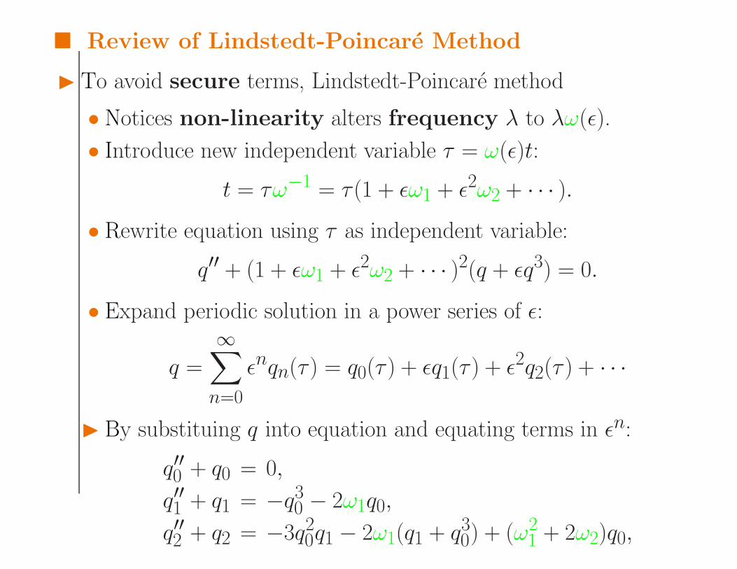
I To avoid secure terms, Lindstedt-Poincare method

• Notices non-linearity alters frequency λ to λω(ε).• Introduce new independent variable τ = ω(ε)t:

t = τω−1 = τ (1 + εω1 + ε2ω2 + · · · ).• Rewrite equation using τ as independent variable:

q′′ + (1 + εω1 + ε2ω2 + · · · )2(q + εq3) = 0.

• Expand periodic solution in a power series of ε:

q =∞∑n=0

εnqn(τ ) = q0(τ ) + εq1(τ ) + ε2q2(τ ) + · · ·

I By substituing q into equation and equating terms in εn:

q′′0 + q0 = 0,q′′1 + q1 = −q30 − 2ω1q0,

q′′2 + q2 = −3q20q1 − 2ω1(q1 + q30) + (ω21 + 2ω2)q0,

Review of Lindstedt-Poincare Method

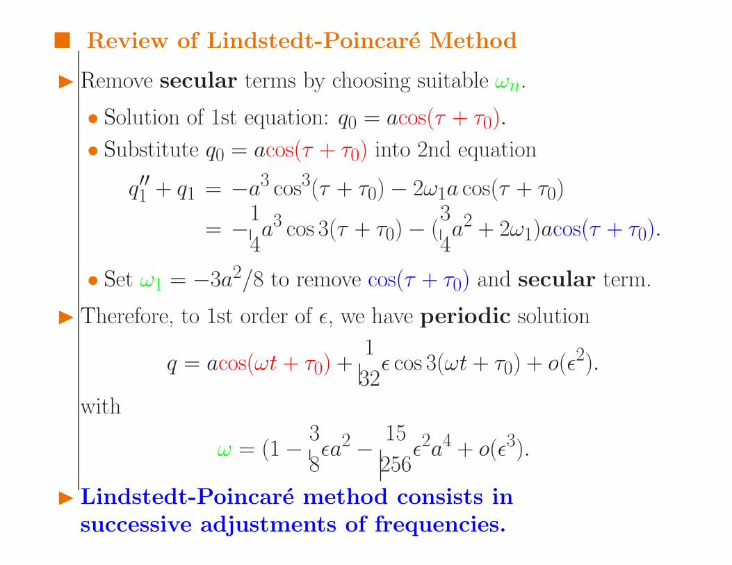
I Remove secular terms by choosing suitable ωn.

• Solution of 1st equation: q0 = acos(τ + τ0).• Substitute q0 = acos(τ + τ0) into 2nd equation

q′′1 + q1 = −a3 cos3(τ + τ0) − 2ω1a cos(τ + τ0)

= −14a3 cos 3(τ + τ0) − (

34a2 + 2ω1)acos(τ + τ0).

• Set ω1 = −3a2/8 to remove cos(τ + τ0) and secular term.

I Therefore, to 1st order of ε, we have periodic solution

q = acos(ωt + τ0) +132ε cos 3(ωt + τ0) + o(ε2).

with

ω = (1 − 38εa2 − 15

256ε2a4 + o(ε3).

I Lindstedt-Poincare method consists insuccessive adjustments of frequencies.

Lindstedt Poincare Method: Nonlinear Expansion

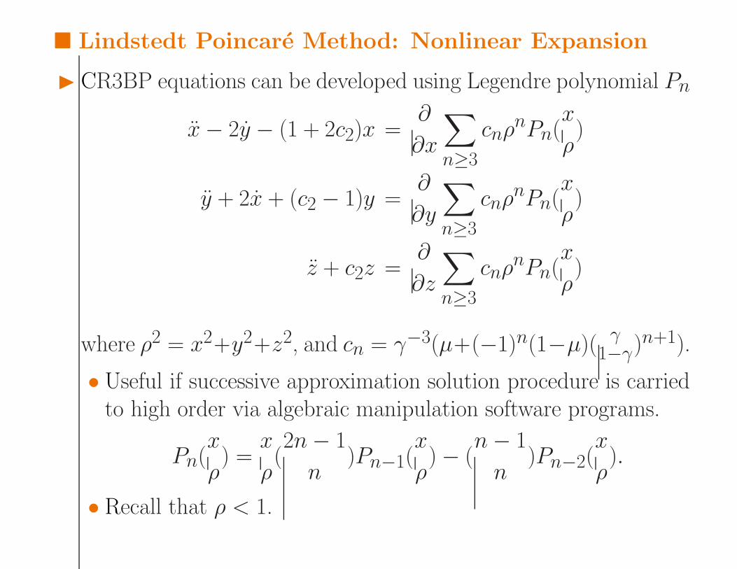
I CR3BP equations can be developed using Legendre polynomial Pn

x− 2y − (1 + 2c2)x =∂

∂x

∑n≥3

cnρnPn(

x

ρ)

y + 2x + (c2 − 1)y =∂

∂y

∑n≥3

cnρnPn(

x

ρ)

z + c2z =∂

∂z

∑n≥3

cnρnPn(

x

ρ)

where ρ2 = x2+y2+z2, and cn = γ−3(µ+(−1)n(1−µ)( γ1−γ)n+1).

• Useful if successive approximation solution procedure is carriedto high order via algebraic manipulation software programs.

Pn(x

ρ) =

x

ρ(2n− 1n

)Pn−1(x

ρ) − (

n− 1n

)Pn−2(x

ρ).

• Recall that ρ < 1.

Lindstedt Poincare Method: 3rd Order Expansion

I 3rd order approximation used in Richardson [1980]:

x− 2y − (1 + 2c2)x =32c3(2x2 − y2 − z2)

+2c4x(2x2 − 3y2 − 3z2) + o(4),

y + 2x + (c2 − 1)y = −3c3xy − 32c4y(4x2 − y2 − z2) + o(4),

z + c2z = −3c3xz − 32c4z(4x2 − y2 − z2) + o(4).

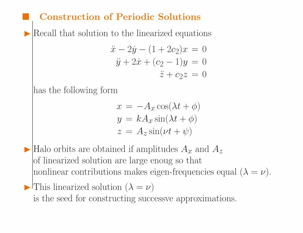
Construction of Periodic Solutions

I Recall that solution to the linearized equations

x− 2y − (1 + 2c2)x = 0y + 2x + (c2 − 1)y = 0

z + c2z = 0

has the following form

x = −Ax cos(λt + φ)y = kAx sin(λt + φ)z = Az sin(νt + ψ)

I Halo orbits are obtained if amplitudes Ax and Azof linearized solution are large enoug so thatnonlinear contributions makes eigen-frequencies equal (λ = ν).

I This linearized solution (λ = ν)is the seed for constructing successve approximations.

Construction of Periodic Solutions

I We would like to rewrite linearized equations in following form:

x− 2y − (1 + 2c2)x = 0y + 2x + (c2 − 1)y = 0

z + λ2z = 0

which has a periodic solution with frequency λ.

I Need to have a correction term ∆ = λ2 − c2for high order approximations.

z + λ2z = −3c3xz − 32c4z(4x2 − y2 − z2) + ∆z + o(4).

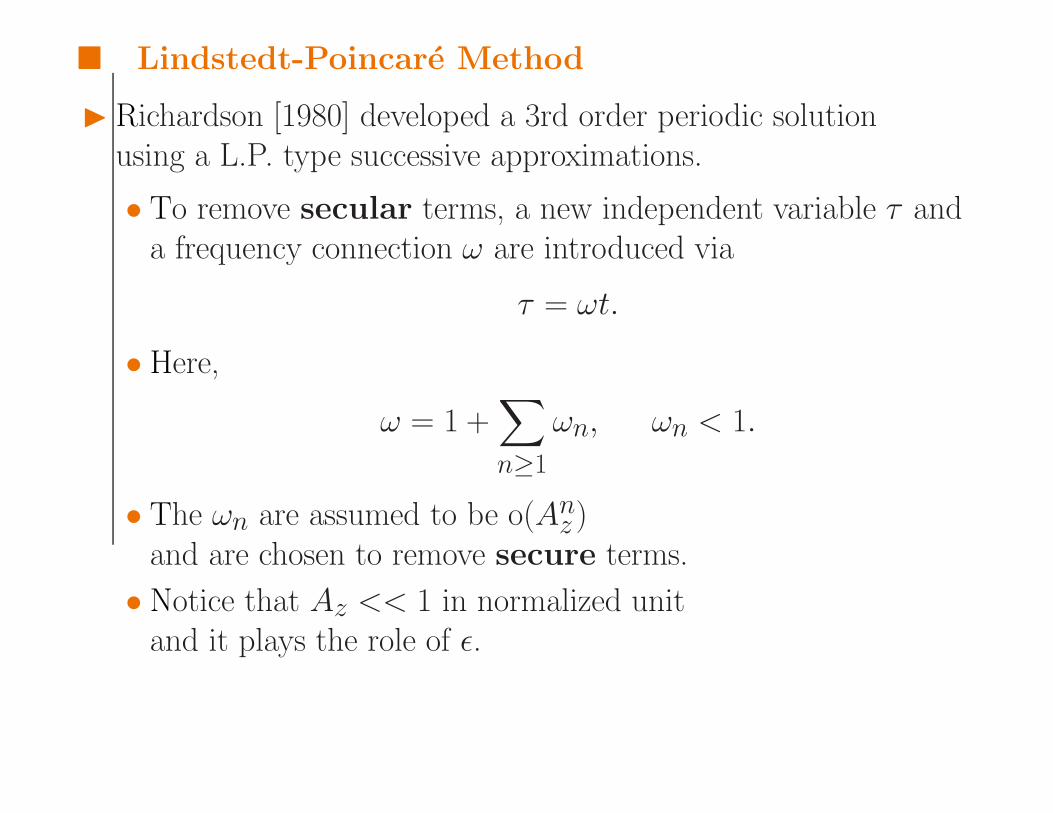
Lindstedt-Poincare Method

I Richardson [1980] developed a 3rd order periodic solutionusing a L.P. type successive approximations.

• To remove secular terms, a new independent variable τ anda frequency connection ω are introduced via

τ = ωt.

• Here,

ω = 1 +∑n≥1

ωn, ωn < 1.

• The ωn are assumed to be o(Anz )and are chosen to remove secure terms.

• Notice that Az << 1 in normalized unitand it plays the role of ε.

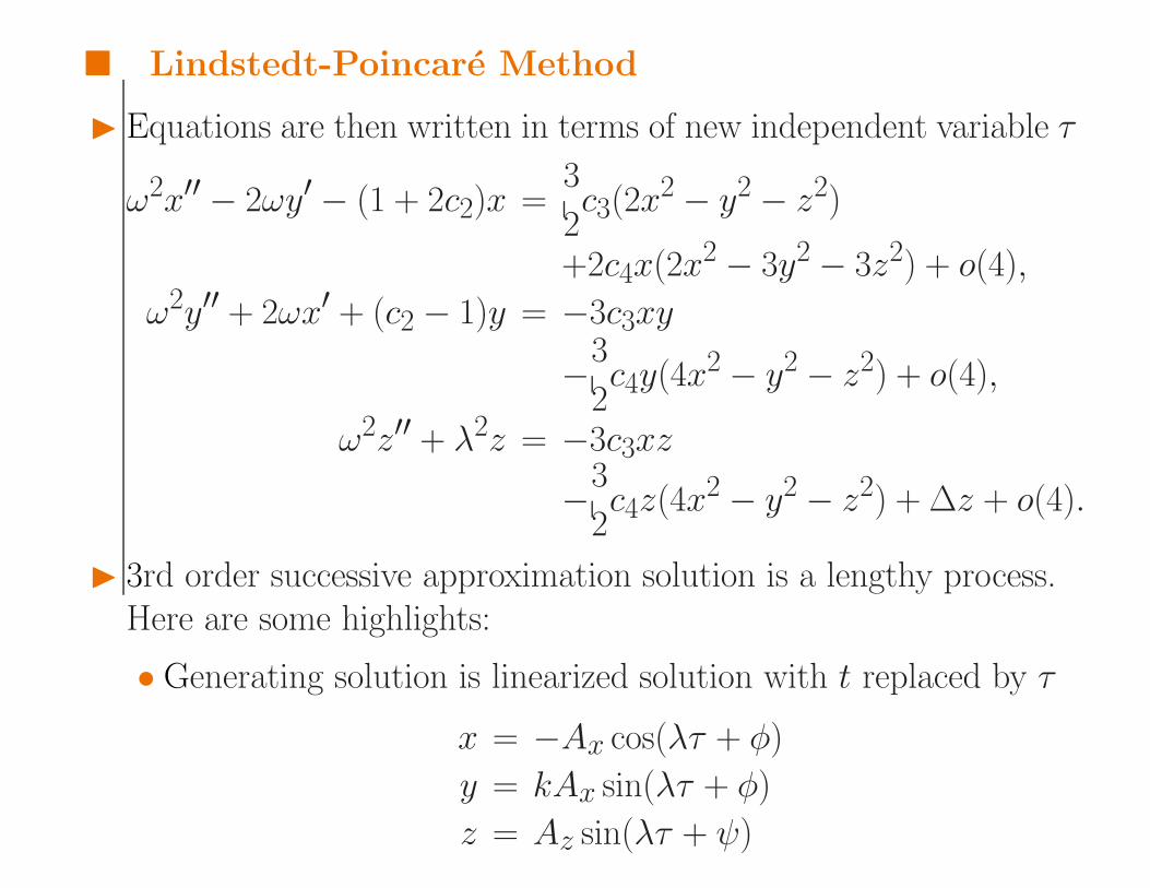
Lindstedt-Poincare Method

I Equations are then written in terms of new independent variable τ

ω2x′′ − 2ωy′ − (1 + 2c2)x =32c3(2x2 − y2 − z2)

+2c4x(2x2 − 3y2 − 3z2) + o(4),ω2y′′ + 2ωx′ + (c2 − 1)y = −3c3xy

−32c4y(4x2 − y2 − z2) + o(4),

ω2z′′ + λ2z = −3c3xz

−32c4z(4x2 − y2 − z2) + ∆z + o(4).

I 3rd order successive approximation solution is a lengthy process.Here are some highlights:

• Generating solution is linearized solution with t replaced by τ

x = −Ax cos(λτ + φ)y = kAx sin(λτ + φ)z = Az sin(λτ + ψ)

Lindstedt-Poincare Method

I Some highlights:

• Look for general solutions of the following type:

x =∑n≥0

an cosnτ1, y =∑n≥0

bn sinnτ1, z =∑n≥0

cn cosnτ1,

where τ1 = λτ + φ = λωt + φ.• It is found that

ω1 = 0, ω2 = s1A2x + s2A

2z,

which give the frequence λω (ω = 1 + ω1 + ω2 + · · · ) and theperiod T (T = 2π/λω) of a halo orbit.

• To remove all secular terms, it is also necessary to specifyamplitude and phase-angle constraint relationships:

l1A2x + l2A

2z + ∆ = 0,ψ − φ = mπ/2, m = 1, 3.

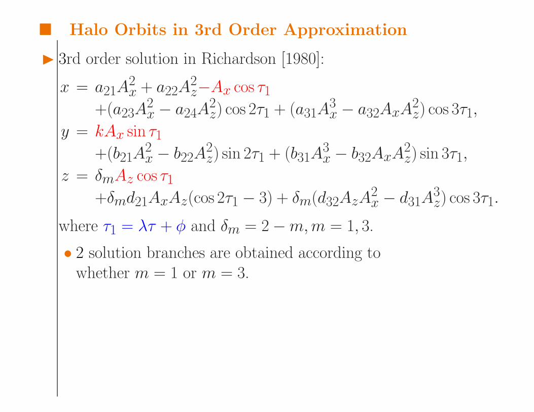
Halo Orbits in 3rd Order Approximation

I 3rd order solution in Richardson [1980]:

x = a21A2x + a22A

2z−Ax cos τ1

+(a23A2x − a24A

2z) cos 2τ1 + (a31A

3x − a32AxA

2z) cos 3τ1,

y = kAx sin τ1+(b21A

2x − b22A

2z) sin 2τ1 + (b31A

3x − b32AxA

2z) sin 3τ1,

z = δmAz cos τ1+δmd21AxAz(cos 2τ1 − 3) + δm(d32AzA

2x − d31A

3z) cos 3τ1.

where τ1 = λτ + φ and δm = 2 −m,m = 1, 3.

• 2 solution branches are obtained according towhether m = 1 or m = 3.

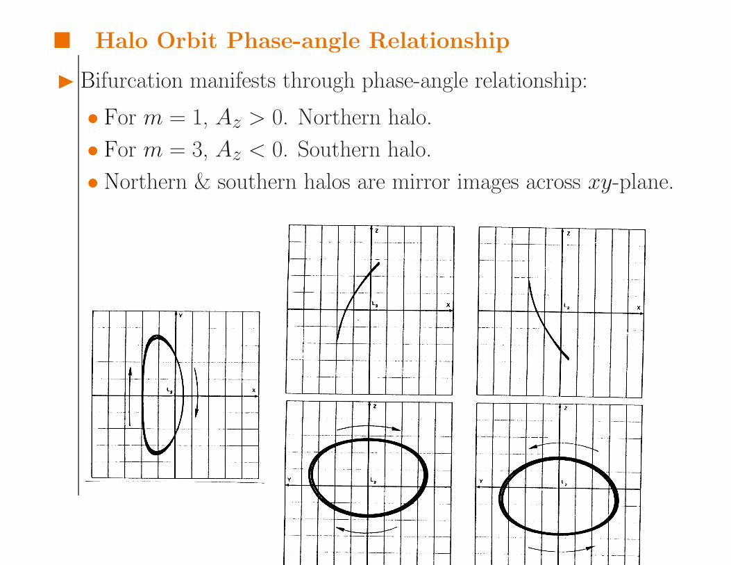
Halo Orbit Phase-angle Relationship

I Bifurcation manifests through phase-angle relationship:

• For m = 1, Az > 0. Northern halo.• For m = 3, Az < 0. Southern halo.• Northern & southern halos are mirror images across xy-plane.

Halo Orbit Amplitude Constraint Relationship

I For halo orbits, we have amplitude constraint relationship

l1A2x + l2A

2z + ∆ = 0.

• Minimim value for Ax to have a halo orbit (Az > 0) is√|∆/l1|,

which is about 200, 000 km.• Halo orbit can be characterized completely by Az.

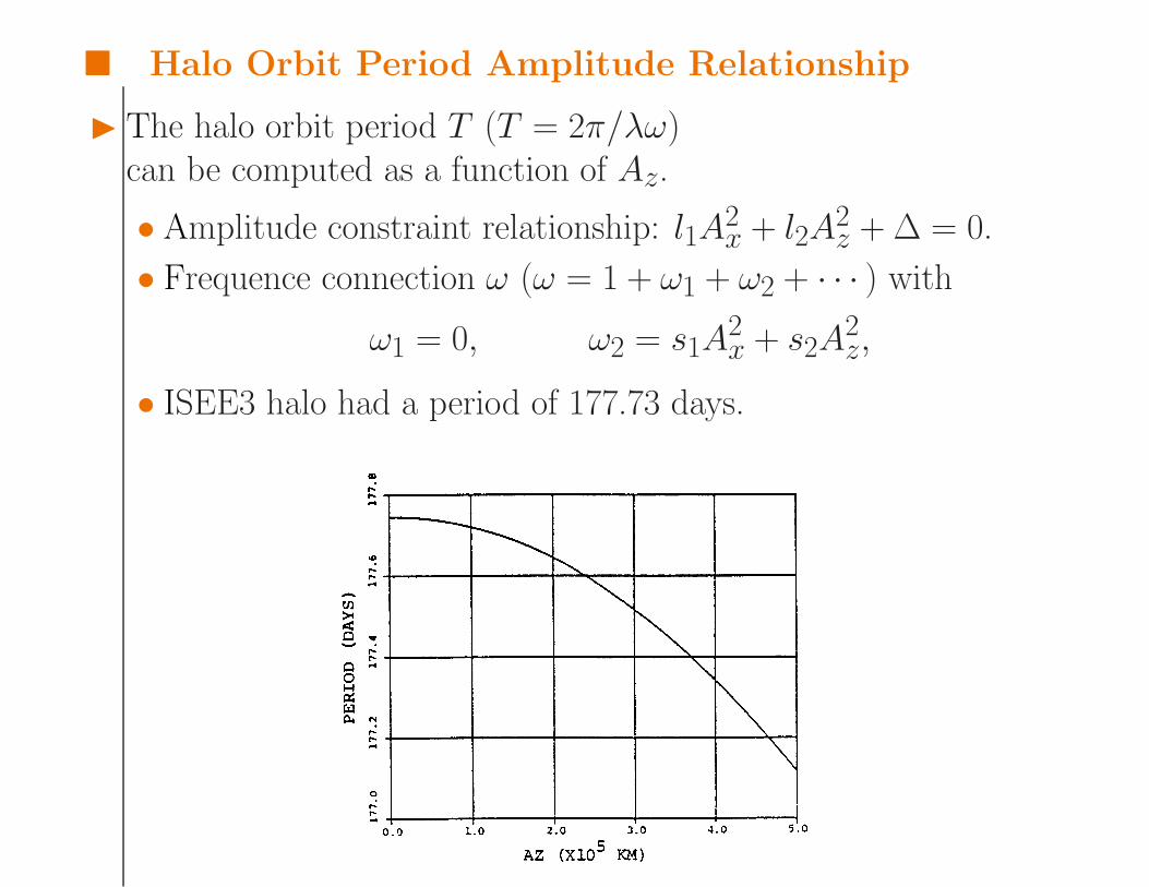
Halo Orbit Period Amplitude Relationship

I The halo orbit period T (T = 2π/λω)can be computed as a function of Az.

• Amplitude constraint relationship: l1A2x + l2A

2z + ∆ = 0.

• Frequence connection ω (ω = 1 + ω1 + ω2 + · · · ) with

ω1 = 0, ω2 = s1A2x + s2A

2z,

• ISEE3 halo had a period of 177.73 days.

Differential Corrections

I While 3rd order approximations provide much insight,they are insufficient for serious study of motion near L1.

I Analytic approximations must be combined withnumerical techniques to generate an accurate halo orbit.

I This problem is well suited to a differential corrections process,

• which incorporates the analytic approximationsas the first guess

• in an iterative process• aimed at producing initial conditions that lead to a halo orbit.

Differential Corrections: Variational Equations

I Recall 3D CR3BP equations:

x− 2y = Ux y + 2x = Uy z = Uz

where U = (x2 + y2)/2 + (1 − µ)d−11 + µd−1

2 .

I It can be rewritten as 6 1st order ODEs: ˙x = f (x),where x = (x y z x y z)T is the state vector.

I Given a reference solution x to ODE,

• variational equations which are linearized equations forvariations δx (relative to reference solution) can be written as

˙δx(t) = Df (x)δx = A(t)δx(t),

where A(t) is a matrix of the form[0 I3U 2Ω

].

Differential Corrections: Variational Equations

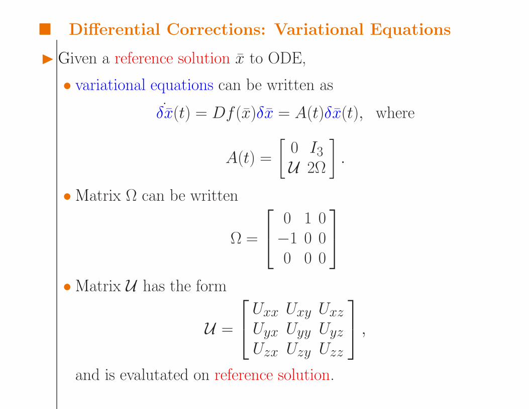
I Given a reference solution x to ODE,

• variational equations can be written as˙δx(t) = Df (x)δx = A(t)δx(t), where

A(t) =[

0 I3U 2Ω

].

• Matrix Ω can be written

Ω =

0 1 0

−1 0 00 0 0

• Matrix U has the form

U =

Uxx Uxy UxzUyx Uyy UyzUzx Uzy Uzz

,

and is evalutated on reference solution.

Differential Corrections: State Transition Matrix

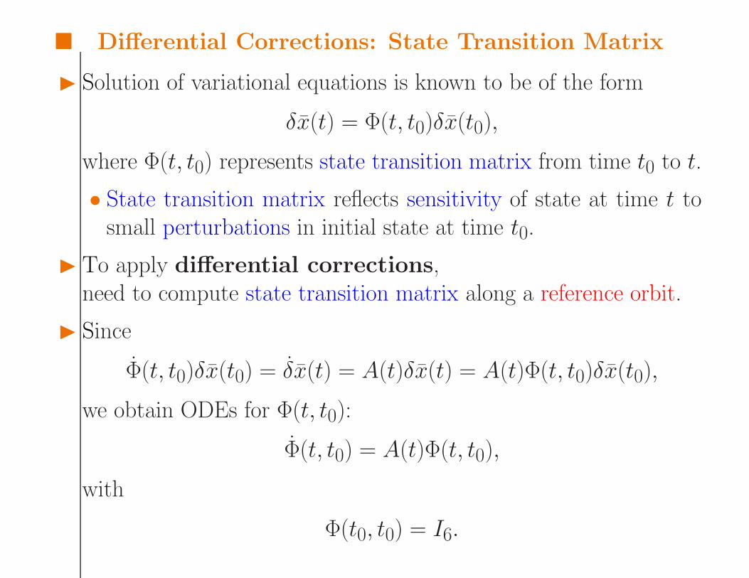
I Solution of variational equations is known to be of the form

δx(t) = Φ(t, t0)δx(t0),

where Φ(t, t0) represents state transition matrix from time t0 to t.

• State transition matrix reflects sensitivity of state at time t tosmall perturbations in initial state at time t0.

I To apply differential corrections,need to compute state transition matrix along a reference orbit.

I Since

Φ(t, t0)δx(t0) = δx(t) = A(t)δx(t) = A(t)Φ(t, t0)δx(t0),

we obtain ODEs for Φ(t, t0):

Φ(t, t0) = A(t)Φ(t, t0),

with

Φ(t0, t0) = I6.

Differential Corrections: State Transition Matrix

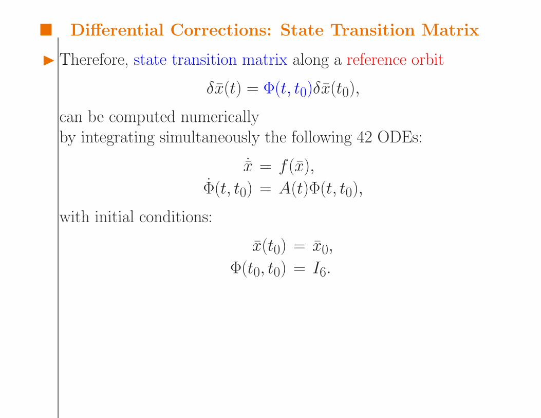
I Therefore, state transition matrix along a reference orbit

δx(t) = Φ(t, t0)δx(t0),

can be computed numericallyby integrating simultaneously the following 42 ODEs:

˙x = f (x),Φ(t, t0) = A(t)Φ(t, t0),

with initial conditions:

x(t0) = x0,

Φ(t0, t0) = I6.

Numerical Computation of Halo Orbit

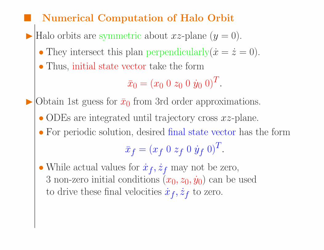
I Halo orbits are symmetric about xz-plane (y = 0).

• They intersect this plan perpendicularly(x = z = 0).• Thus, initial state vector take the form

x0 = (x0 0 z0 0 y0 0)T .

I Obtain 1st guess for x0 from 3rd order approximations.

• ODEs are integrated until trajectory cross xz-plane.• For periodic solution, desired final state vector has the form

xf = (xf 0 zf 0 yf 0)T .

• While actual values for xf , zf may not be zero,3 non-zero initial conditions (x0, z0, y0) can be usedto drive these final velocities xf , zf to zero.

Numerical Computation of Halo Orbit

I Differential corrections use state transition matrixto change initial conditions

δxf = Φ(tf , t0)δx0.

• The change δx0 can be determined by the difference betweenactual and desired final states (δxf = xdf − xf ).

• 3 initial states (δx0, δz0, δy0)are available to target 2 final states (δxf , δzf ).

• But it is more convenient to set δz0 = 0and to use resulting 2 × 2 matrix to find δx0, δy0.

I Similarly, the revised initial conditions x0 + δx0are used to begin a second iteration.

I This process is continued until xf = zf = 0(within some accptable tolerance).

• Usually, convergence to a solution is achieved within 4 iterations.

Numerical Computation of Lissajous Trajectories

I Howell and Pernicka [1987] used similar techniques(3rd order approximation and differential corrections)to compute lissajous trajectories.

I Gomez, Jorba, Masdemont and Simo [1991] usedhigher order expansions to compute halo, quasi-halo and lissajousorbits.

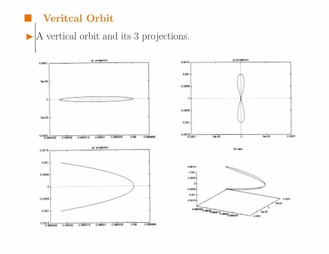
Veritcal Orbit

I A vertical orbit and its 3 projections.

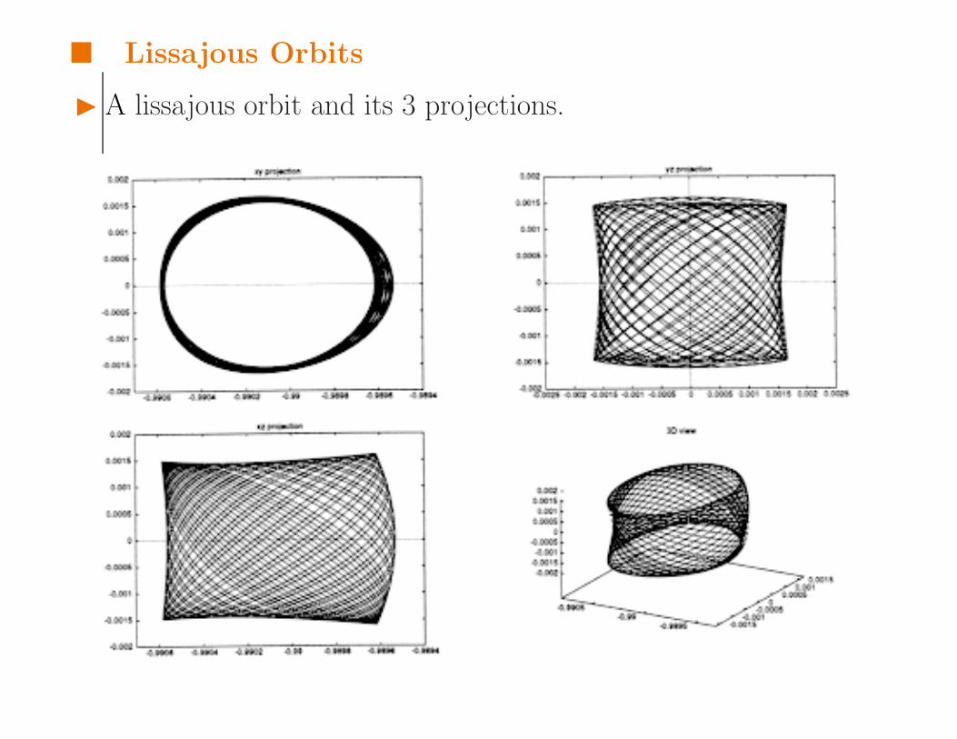
Lissajous Orbits

I A lissajous orbit and its 3 projections.

Halo Orbits

I A halo orbit and its 3 projections.

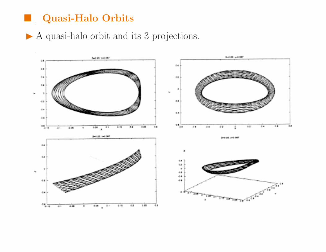
Quasi-Halo Orbits

I A quasi-halo orbit and its 3 projections.

Orbit Structure around L1

I Poincare sections of center manifold of L1 corresponding to h =0.2, 0.5, 0.6, 1.0.