contribution to the optimised design of combined piled ... · diploma thesis contribution to the...
TRANSCRIPT

Diploma Thesis
Contribution to the optimised design of
combined piled raft foundations (CPRF)
Submitted in satisfaction of the requirements for the degree of
Diplom-Ingenieur
of the TU Wien, Faculty of Civil Engineering
Diplomarbeit
Beitrag zur optimierten Bemessung von Kombinierten Pfahl-Plattengründungen (KPP)
ausgeführt zum Zwecke der Erlangung des akademischen Grades eines
Diplom-Ingenieurs
eingereicht an der Technischen Universität Wien, Fakultät für Bauingenieurwesen
von
Corentin Dufour Matr.Nr.: 01623360
unter der Anleitung von
Univ.-Prof. Dipl.-Ing. Dr.techn. Dietmar Adam
Univ.-Ass. Dipl.-Ing. Péter Nagy, B.Sc
Institut für Geotechnik Forschungsbereich für Grundbau, Boden- und Felsmechanik
Technische Universität Wien, Karlsplatz 13/220-02, A-1040 Wien
in Zusammenarbeit mit und Betreuung durch
STRABAG SE, Zentrale Technik Donau-City-Str. 9, 1220 Wien
Dipl.-Ing. Dipl.-Ing. Dr.-Ing. Maximilian Huber
Wien, im Juni 2018


Preface
The work presented in this master thesis is the result of a cooperation between the Institute of
Geotechnical Engineering of the Technical University of Vienna and the company STRABAG SE. It is
part of a double degree with the École Centrale de Lyon (France).
I would like to thank all the people that made this work possible sincerely, hence all those who supported
me during the writing process of my master thesis and who contributed to its achievement.
Furthermore, I wish to express my profound gratitude to my supervisor at the STRABAG Dr.-Ing
Maximilian Huber for his extensive, invaluable and steadfast guidance. Thank you for sharing your
knowledge and experience with me, for your interest in my work and for your willingness to answer my
questions. Your critical view on the problem addressed in this paper made me think even more critically.
In particular I would like to thank Prof. Dietmar Adam, who gave me the opportunity to do my research
project under his supervision, and whose effort and time to review my entire work enabled me to
improve the quality of my thesis.
I especially thank Dipl.-Ing. Péter Nagy for his availability and his help regarding various subjects, i.e.
both technical and administrative aspects. Thank you for your support and the supply of important
documentation as well as for your pertinent remarks on my work.
I would also like to thank Dipl.-Ing Thomas Wieser, who enabled this cooperation thanks to the financial
support of the STRABAG and who agreed on the exciting subject of the master thesis.
Likewise, I thank all the colleagues of the Zentrale Technik and in particular Dipl.-Ing Emir Ahmetovic
for the positive working environment, which motivated me to accomplish this work.
I am very grateful to Christine Mascha for her answers to my numerous questions throughout my study
at the Technical University of Vienna and especially during my master thesis.
I also wish to express my heartfelt thanks to Mag. Barbara Fussi, Alastair Gardner, Mag. René
Guggelberger, Mag. Anna Heidlmair, Mag. Michaela Reisner and Mag. Stefanie Trappl for their
percipient and accurate proofreading of my master thesis.
All of this would not have been possible without the unconditional support of my family and friends
throughout my whole studies. To them I would like to express my sincere gratitude.


Abstract
An increasing share of the population lives and works in cities. It is widely expected that these patterns
persist as urban areas account for a greater share of activity. This asks for high rise buildings and
advanced foundations systems, which are able to transfer high loads from the ground surface into deep
layers.
This master thesis focuses on the optimisation of combined piled raft foundations (CPRFs), which are
hybrid foundation systems combining the bearing capacity of a foundation raft with the piles. Elements
of the foundation exercise a mutual load-bearing effect and present reciprocal interactions as well as
interactions with the subsoil. Herein both a semi-analytical approach for the simulation of soil structure
interaction and a multi-objective optimisation to minimise the required resources for the deep foundation
are used. After outlining the semi-analytical model for the design of pile groups and CPRFs, it is applied
in a standard CPRF benchmark from the literature. The obtained design is then optimised using genetic
algorithms.
This new design approach enables a rapid and robust semi-analytical approximation of the load-bearing
behaviour of the structure, which can facilitate the calculation and cost estimation of projects in the
tender phase. It is further implemented in a script capable of an optimised design covering geotechnical
as well as structural aspects. By using multi-objective optimisation, better and more cost-effective
results have been achieved compared to reference solutions presented in the literature. As far as the
overall need for concrete masses for the raft and the piles is concerned, the obtained solutions show
significant reduction of required concrete. The findings of these analyses contribute to the cost efficient
design of foundation systems combining the need of practical engineering, advanced soil mechanical
approaches and optimisation techniques.
It has further been shown that a direct relation between costs and settlement can be established and
displayed in the form of a Pareto front. This finding facilitates the evaluation of the possible cost savings
with a concrete insight into the increased risks following those savings. The representation of a Pareto
front enables a rapid cost-benefit analysis. This optimisation procedure represents a new perspective for
constructors and planners, which opens the way for more competitive solutions in foundation design
and fosters the optimisation of complex problems in civil engineering.


Kurzfassung
Ein zunehmender Teil der Bevölkerung lebt und arbeitet in Städten. Es ist zu erwarten, dass diese
Tendenz fortdauert, da sich in Ballungsräume ein erheblicher Teil der Wirtschaftstätigkeit konzentriert.
Der steigende Wohnraumbedarf in Großstädten bei hohen Grundstückspreisen führt unter anderem zum
Bau von Hochhäusern in Ballungsräumen. Diese Hochhäuser fordern hochentwickelte Gründungen, die
die hohen Lasten von der Gründungsoberfläche in tiefliegende Bodenschichten übertragen können.
Im Rahmen der vorliegenden Diplomarbeit wurden die Kombinierten Pfahl-Plattengründungen (KPP)
behandelt. KPP sind geotechnische Verbundkonstruktionen mit gemeinsamer Tragwirkung von
Fundamentplatte und Pfählen, die komplexe Wechselwirkungen aufweisen, sowohl zwischen den
einzelnen Strukturelementen als auch mit dem Boden. Ein semi-analytisches Berechnungsverfahren
wurde für die Abschätzung der Boden-Bauwerk Interaktion durchgeführt. Weiterhin wurde eine
multikriterielle Optimierung für die Reduzierung der erforderlichen Ressourcen der Gründung
entwickelt. Nachdem das semi-analytische Berechnungsverfahren für Pfahlgruppen und KPP
hervorgehoben wird, wird es mit erprobten Beispielen aus der Literatur verglichen. Der daraus
resultierende Entwurf wird schlussendlich optimiert mittels genetischer Algorithmen.
Dieses neue Verfahren ermöglicht eine schnelle und robuste Näherung des Tragverhaltens der
Gründung, das die Kostenermittlung und die Berechnung in der Ausschreibungsphase unterstützen
kann. Zudem wird das Verfahren in einem Skript abgeleitet, welches sowohl die geotechnische als auch
die konstruktive Bemessung abdeckt. Anhand multikriterieller Optimierung wurden kosteneffektivere
Lösungen als jene der Literatur ermittelt. Die Menge an erforderlichen Baumaterial konnte reduziert
werden, ohne die Fähigkeiten des Trageverhaltens zu verringern. Die Ergebnisse dieser Analyse tragen
zum kosteneffektiven Design von KPP bei.
Darüber hinaus wurde gezeigt, dass mit Hilfe eines evolutionären Algorithmus eine direkte Verbindung
zwischen optimaler Setzung und minimalen Kosten abgeleitet und mittels einer Paretofront dargestellt
werden kann. Auf die Gefahr hin, dass die Setzungen zunehmen, kann so festgestellt werden, welche
Kosteneinsparungen möglich ist. Die Darstellung der Paretofront ermöglicht außerdem eine schnelle
Kosten-Nutzen-Analyse. Dies eröffnet eine neue Sichtweise für BaumeisterInnen und PlanerInnen und
fördert sowohl die Planung kompetitiver Lösungen als auch die Optimierung von komplexen Problemen
im Bauwesen.


Résumé
Une part croissante de la population vit et travaille dans les villes et il est très probable que cette tendance
persiste étant donné que les aires urbaines concentrent une grande part de l’activité économique. Ce
phénomène conduit à un développement des gratte-ciels et des superstructures, édifices nécessitant des
fondations capables de transférer de fortes charges de la surface de la fondation jusqu’à des couches de
sol plus profondes.
Le présent mémoire se penche sur l’optimisation de fondations mixtes radier-pieux, fondations hybrides
combinant la capacité portante d’un radier avec celle d’un groupe de pieux. Les éléments de cette
fondation exercent un effet mutuel de portance et présentent des interactions complexes radier-pieux-
sol. Une approche semi-analytique pour la simulation de l’interaction sol-structure ainsi qu’une
optimisation multi objectifs pour minimiser la quantité de ressources nécessaire sont effectués. Après
avoir mis en avant le modèle semi-analytique développé pour modéliser les groupes de pieux et les
fondations mixtes, celui-ci est appliqué à des cas concrets pour pouvoir comparer les résultats à ceux
obtenus numériquement par diverses études scientifiques. Le design est ensuite optimisé par
l’intermédiaire d’algorithmes génétiques.
Cette nouvelle approche de conception permet une approximation rapide et robuste de la capacité
portante de la structure, ce qui aide au dimensionnement de la fondation et à l’estimation des coûts lors
des procédures d’appel d’offre ou pour concevoir un design préliminaire. Le modèle est implémenté
dans un script couvrant aussi bien les aspects géotechniques que structurels. A l’aide d’une optimisation
multi-objectif, des résultats plus économiques que ceux obtenus numériquement ont pu être obtenus.
Les résultats montrent en effet une réduction significative de la quantité de béton nécessaire pour des
performances similaires.
Une relation directe entre le coût de la structure et le tassement, représentée au moyen d’un optimum de
Pareto, a par ailleurs été obtenue. Il est ainsi plus facile d’évaluer quelles économies peuvent être
effectuées sans pour autant affecter la sécurité de la fondation. Cette représentation sous forme de
frontière d’efficacité de Pareto permet une analyse coûts-avantages rapide. La procédure d’optimisation
développée représente une nouvelle perspective pour les constructeurs et les bureaux d’études, qui ouvre
la voie à des solutions plus compétitives concernant la conception des fondations et l’optimisation de
problèmes complexes du génie civil.


Table of contents
1 Introduction 15
1.1 Scope of the thesis and research objective ............................................................................ 15
1.2 Methodology ......................................................................................................................... 16
1.2.1 Literature study .................................................................................................................. 17
1.2.2 Pile group and CPRF design .............................................................................................. 17
1.2.3 Optimisation ...................................................................................................................... 18
1.2.4 Calculation programs......................................................................................................... 18
2 Pile Foundation Systems 19
2.1 Single pile .............................................................................................................................. 19
2.2 Pile grillage............................................................................................................................ 20
2.3 Pile group .............................................................................................................................. 20
2.4 Combined piled raft foundation............................................................................................. 23
3 Pile group design 27
3.1 Literature review on pile group design .................................................................................. 27
3.1.1 Empirical methods ............................................................................................................. 28
3.1.2 Analytical methods ............................................................................................................ 29
3.1.3 Numerical methods ............................................................................................................ 30
3.2 Design approach after Rudolph (2005) ................................................................................. 31
3.2.1 Assumptions ...................................................................................................................... 31
3.2.2 Flexibility coefficients ....................................................................................................... 31
3.2.3 Equilibrium of the pile group ............................................................................................ 32
3.2.4 Influence radius ................................................................................................................. 33
3.2.5 Failure criterion ................................................................................................................. 34
3.2.6 Workflow ........................................................................................................................... 35
3.3 Modifications and improvements .......................................................................................... 38
3.3.1 Accuracy of the influence radius ....................................................................................... 38
3.3.2 Comparison of flexibility coefficients ............................................................................... 39
3.3.3 Soil stiffness ...................................................................................................................... 41
3.3.4 Loading cases .................................................................................................................... 42
3.3.5 Geometrical parameters ..................................................................................................... 43
3.3.6 Differential settlement ....................................................................................................... 43

12 Table of contents
3.3.7 Object oriented programming ............................................................................................ 45
3.3.8 Workflow ........................................................................................................................... 45
3.4 Limitations and drawbacks .................................................................................................... 46
4 Design of combined piled raft foundation 49
4.1 Literature review on piled raft foundations ........................................................................... 49
4.1.1 Equivalent models ............................................................................................................. 49
4.1.2 Empirical methods ............................................................................................................. 49
4.1.3 Analytical methods ............................................................................................................ 50
4.1.4 Numerical methods ............................................................................................................ 52
4.2 Design procedure for PRF ..................................................................................................... 53
4.2.1 Area of application ............................................................................................................ 53
4.2.2 Calculation method requirements for PR design ............................................................... 53
4.2.3 Ultimate Limit State - ULS ............................................................................................... 54
4.2.4 Serviceability Limit State - SLS ........................................................................................ 56
4.2.5 Piled raft monitoring.......................................................................................................... 57
4.3 Adopted design approach ...................................................................................................... 58
4.3.1 Modelling of the raft-soil interaction................................................................................. 58
4.3.2 System rigidity .................................................................................................................. 59
4.3.3 Workflow ........................................................................................................................... 61
4.4 Limitations and drawbacks .................................................................................................... 62
5 Case studies on pile groups and piled raft foundations 63
5.1 Pile groups ............................................................................................................................. 64
5.1.1 Guideline 1.2 ..................................................................................................................... 64
5.1.2 End bearing pile and skin friction pile............................................................................... 68
5.2 Combined piled raft foundation............................................................................................. 70
6 Optimisation of pile groups and piled raft foundations 77
6.1 Optimisation method ............................................................................................................. 77
6.1.1 Problem ............................................................................................................................. 77
6.1.2 Population .......................................................................................................................... 78
6.1.3 Algorithm .......................................................................................................................... 78
6.2 Optimisation of pile groups ................................................................................................... 81
6.2.1 Design parameters ............................................................................................................. 82
6.2.2 Objective functions ............................................................................................................ 82
6.2.3 Constraints and box boundaries ......................................................................................... 82
6.2.4 Results ............................................................................................................................... 82

Table of contents 13
6.3 Optimisation of CPRFs ......................................................................................................... 84
6.3.1 Rigidity .............................................................................................................................. 84
6.3.2 Box boundaries .................................................................................................................. 85
6.3.3 Results ............................................................................................................................... 86
6.4 Limitations and drawbacks .................................................................................................... 89
7 Summary and conclusions 91
References 93
Table of figures 97
Table of charts 99
Appendix A Python Codes 101
A.1 Analytical calculation of a pile group .................................................................................... 101
A.2 Multi-optimisation of a pile group ......................................................................................... 112
Appendix B Global and partial safety concept 115
B.1 Global safety concept ............................................................................................................. 115
B.2 Partial safety factor concept ................................................................................................... 115
B.3 Comparison of the two concepts ............................................................................................ 117
Appendix C Optimisation 119
C.1 Academic benchmark ............................................................................................................. 119
C.2 Choice of the algorithm .......................................................................................................... 121


1 Introduction
1.1 Scope of the thesis and research objective Cities are often seen as centres of economic growth, providing opportunities for study, innovation and
employment. The growing housing space demand in cities combined with a steep rise in real estate leads
to the development of more and more high-rise buildings in city centres. Amongst others, this is the case
in Frankfurt am Main, Germany, where numerous skyscrapers were constructed in the last decades (see
Figure 1.1).
Design, construction and performance of these superstructures largely rely on the stability of their
foundations. Deep foundations are often necessary to transfer loads of such major structures in the
subsoil. A possible alternative to these foundations is a combination of elements of shallow foundations
on the one hand with elements of deep foundations, on the other hand, forming the so-called Combined
Piled-Raft Foundations (CPRF). A CPRF is thus a geotechnical composite construction coupling the
bearing effect of both foundation elements raft and piles.
Major advantages of combined piled raft foundations are lower settlements of the whole structure as
well as a reduction of the volume of material used in comparison with deep foundations, leading to
optimised cost and better economic viability. Thus, such foundations are often chosen for highly loaded
buildings or bridge foundations.
This master thesis aims at developing an algorithm capable of a quick, robust and optimised design of
CPRFs covering the basic geotechnical as well as structural aspects. This algorithm should be a smart
and efficient tool, which allows a rapid and simple adaptation of the local boundary conditions. The
calculation time should not exceed some seconds. It should include elaborated approaches such as a
non-homogeneous soil model with a linearly increasing modulus or the introduction of a failure
criterion. Consequently, the developed algorithm would offer an evolved design but would remain quick
and easy to handle.
Figure 1.1: Development of recent high-rise buildings in Frankfurt am Main, after [31].
16 1 Introduction
This algorithm would be suitable for the preliminary and tender design of a project. Depending on the
legal details of the tender documents, one should be able to change the construction concept, the
construction material and the static system of a high-rise building in order to meet the required design
specifications. The most important purpose of the tender phase is the development of a safe structure
with the smallest possible price. However, for detailed analyses and final design, it is recommended to
have recourse to numerical methods [24], which are the only ones capable of a realist and trustworthy
enough design.
The simplified design of CPRF should be automatized in the developed algorithm so that the calculation
can be applied easily and quickly to various projects. This new design approach enables a rapid semi-
analytical approximation of the load-bearing behaviour of the structure. In combination with standard
structural analysis software such as RFEM, it allows the design of CPRFs after the state of the art.
Developing the algorithm with the programming language Python (see Section 1.2.4) allowed to achieve
this simplified design process.
Moreover, this semi-analytical calculation method is optimised using mathematical algorithms to
minimise the volume of construction material as well as the settlement of the foundation, leading to a
set of optimal solutions. This new design strategy is validated through a benchmark comparing the
results with tested calculations coming from the CPRF guidelines.
This master thesis is divided into five main parts. Chapter 2 gives an overall view of several pile
foundation systems, their way of load transfer to the subsoil and the particularities of the different
systems. Chapter 3 covers the design method of pile groups. The thesis is based on a literature study in
order to compare different design and calculation methods. In particular, it outlines how the algorithm
is developed and describes the improvements realised compared to Rudolf (2005) [47]. Chapter 4 deals
with the design of combined piled raft foundations. Different design and calculation methods are
compared and the developed calculation method is described. Chapter 5 contains case studies on pile
groups and CPRFs to test the efficiency and the reliability of the developed solution. A comparison with
tested examples coming from the literature is carried out. Chapter 6 treats the optimisation of pile groups
and combined piled raft foundations to minimise a multi-objective problem using genetic algorithms.
Finally, Chapter 7 summarises the main findings of the thesis and draw conclusions from them.
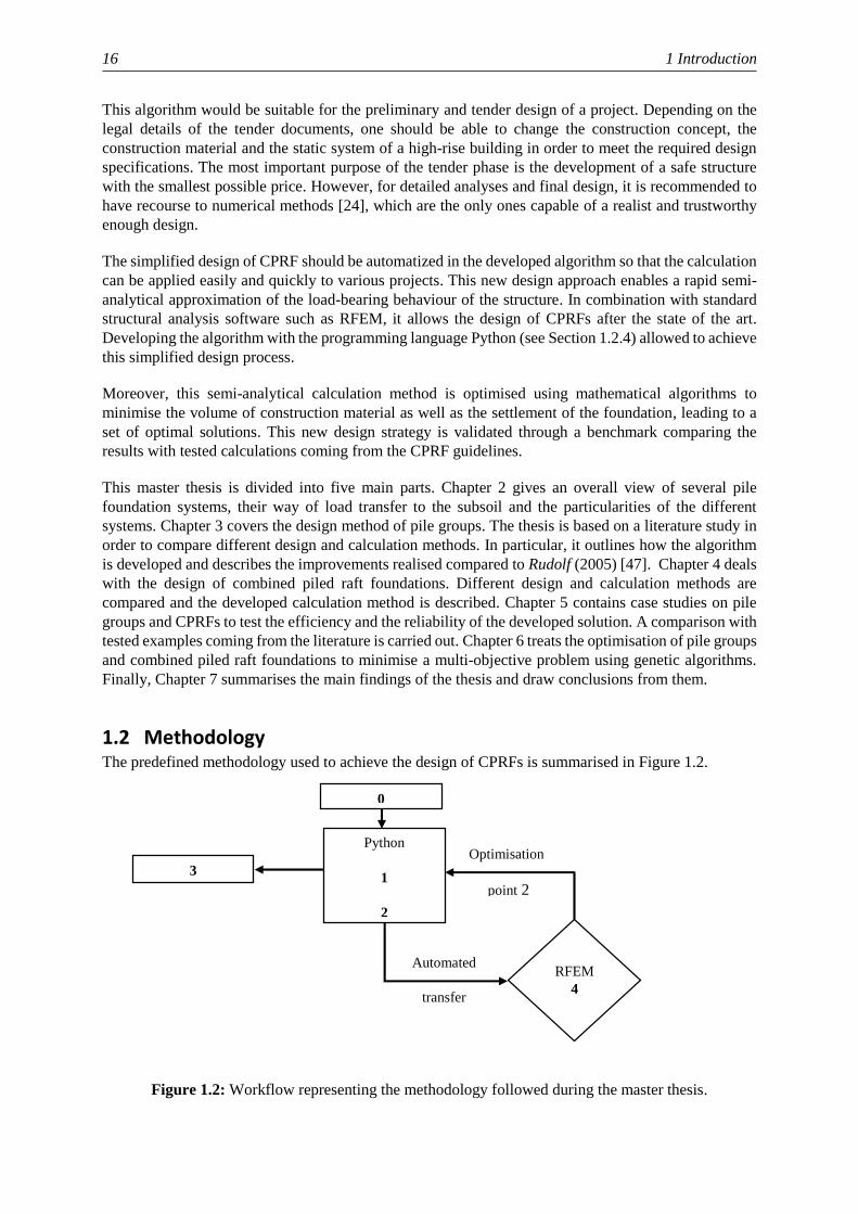
1.2 Methodology The predefined methodology used to achieve the design of CPRFs is summarised in Figure 1.2.
Figure 1.2: Workflow representing the methodology followed during the master thesis.
Automated
transfer
Optimisation
point 2
RFEM
4
RFEM
5
Python
1
2
0
3

1.2 Methodology 17
In Figure 1.2 the following abbreviations are used:
1.2.1 Literature study
A literature study is performed covering, in particular, the concepts of pile group and CPRF design.
Different design approaches are summarised and compared with a special focus on global and partial
safety factor concepts.
The emphasis is put on analytical approximation procedures, and in particular on a comparison regarding
assumptions, expected precision and limits of these procedures. As numerical methods are concerned,
the principal point of interest is the constitutive equations used to model the subsoil.
The study regarding multi-criteria optimisation contains fundaments on mathematical optimisation, pros
and cons of different algorithms, possibilities of the programming language Python to achieve the
requested optimisation as well as advantages of a Pareto front in the cost calculation.
1.2.2 Pile group and CPRF design
An easy way to design CPRF can be achieved following two different possible approaches. One
possibility is to begin the calculation studying exclusively a shallow foundation and to incorporate
elements of deep foundations as well as the resulting interactions afterwards. The other method is to
initiate the calculation with the deep foundation and add the elements of the shallow foundations (such
as the slab) subsequently. The latter solution is chosen for this thesis.
The design process is divided into two major steps: analytical design of a pile group (deep foundation)
followed by a numerical calculation of the slab using the output parameters of the analytical calculation
(i.e. the spring stiffness of each pile). The combination of these two steps provides the desired
calculation of a CPRF. Geotechnical as well as constructive aspects are covered in the algorithm, whose
input parameters are easily modifiable by the user. The analytical design is based on Rudolf (2005) [47],
modified and extended to describe the pile group more realistically and to meet the needs of the current
codes.
As a first step, the analytical calculation of a pile group is coded into a Python framework based on
Rudolf (2005) [47]. Adaptations are made to meet the needs of a fast and simultaneously accurate design
covering the following points:
group effect of a pile group,
stress dependent stiffness,
settlement differences between distinct piles of a group and
non-linear load-bearing behaviour.
The analytical calculation procedure of this algorithm is summarised in a workflow that enables an easier
comprehension of the method (see Figure 3.3). After this, the load-settlement behaviour of the pile group
(and in particular the spring stiffness) is transmitted to the program RFEM to complete the calculation
of the CPRF. The stress resultants of the slab are also evaluated with the help of this structure analysis
0 Literature study,
1 Analytical description of the load-settlement behaviour of a CPR foundation and development of
an adequate Python code,
2 Optimisation of the piles (number, spacing, diameter, length…) using multi- objective optimisation,
3 Benchmark and comparison with the state of the art and
4 Python interface with RFEM.

18 1 Introduction
software. The transfer of the results must be facilitated between Python and RFEM to enable the
dimensioning of the foundation slab, which cannot occur with the analytical calculation in Python.
1.2.3 Optimisation
The use of the language Python to describe the analytical process enables an easy coupling with an
optimisation library also implemented in Python. The modification and the simulation of a multitude of
variables are also made possible with the algorithm.
CPRF optimisation must be based on a robust analytical calculation strategy to offer reliable results. In
fact, no divergence of the calculation should occur during the numerous iteration steps of the
optimisation. That is why a benchmark is necessary, conjointly with a precise study of the relevant input
parameters for each defined CPR to optimise. The multi-criteria optimisation aims at finding optimum
input parameters such as pile length, pile radius, distribution of the position of piles and thickness of the
foundation slab. Those parameters influence the global cubature and in this way the total cost of the
structure. In the end, a Pareto front is to be produced to visualise the set of optimal solutions.
1.2.4 Calculation programs
Different tools are used in this thesis: the structural analysis software RFEM, the programing language
Python and its specific library pygmo.
Python is a universally used high-level, interpreted and dynamic programming language. The design of
its code provides code readability and clear structures. The required syntax is said to be more straight-
forward than the one used in other programming languages. Besides, maintenance is handled easily and
the language is accessible. The version used in the study is Python 3.6.2.
The finite element method program RFEM enables a quick and easy modelling of various structures.
Both static and dynamic calculations are possible with RFEM. Due to its modular software concept, the
basic program can be extended with dedicated modules to meet the needs of each user. The additional
module RF-SOILIN permits, for example, the design of shallow foundations using the subgrade reaction
modulus method. The version used for this work is RFEM 5.11.
Pagmo (implemented in C++) or pygmo (in Python, for PYthon Global Multi-objective Optimizer) is a
scientific library for optimisation problems. It was coded by Izzo and Biscani (2017) [27]. It is built
around the idea of providing a unified interface and enables the use of a multitude of already
implemented algorithms. Its coding style is easy to understand and uses classes to define among others
problems, algorithms and populations. It is strongly recommended to use Anaconda [2] to fulfil the
installation of the pygmo library, making it easy and straightforward. However, Izzo and Biscani (2017)
[27] indicate that pygmo is relatively new and that the syntax of the code may change in the next few
years. Adapting the algorithm in significant proportions may be necessary. The version of pygmo used
in the study is pagmo2-v2.6.

2 Pile Foundation Systems
2.1 Single pile Single piles are piles that do not interact with other piles (or to a negligible degree), neither through the
ground nor the superstructure [33].
When designing piles, one distinguishes between “internal” and “external” pile capacities. The internal
capacity refers to the safety against pile material’s failure (concrete, reinforced concrete, steel, timber,
etc.). As for the external capacity, it refers to the analysis of the safety against failure of the ground
surrounding the pile. According to EC7 [20], both the ultimate limit state (ULS) and the serviceability
limit state (SLS) have to be analysed concerning the internal and the external safety analysis.
Piles can be subject to all types of loading: both vertical and horizontal forces as well as bending
moments. Moreover, the actions may interact with each other to a certain degree. For example, the
application of horizontal forces leads to the apparition of bending moments but also increases the vertical
forces [33]. In most of the cases, however, the non-axial actions are neglected: foundation piles are
predominantly axially loaded.
The axial resistance of a single pile can be divided in two components: the base resistance Rb,k(s) and
the shaft resistance Rs,k(s). The pile resistance is then obtained by summing these two components (see
Equation (2.1). Note that k is the index for the characteristic value.
)s(R)s(R)s(R k,sk,bk,pile (2.1)
The pile shaft resistance Rs,k(s) is calculated as the integral of the skin friction qs,k over the pile skin
surface. The pile base resistance Rb,k(s) as the integral of the end bearing qb,k over the contact area of the
pile base, see Equations (2.2) and (2.3).
4
2Dq)s(R k,bk,b (2.2)
dzD)z,s(q)s(R k,sk,s (2.3)
Both resistances are generally related to the vertical displacements (described by the settlement 𝑠 at the
pile head). They are represented in Figure 2.1 until the settlement limit sg after Katzenbach et al. (2016)
[31].
The settlement limit sg to mobilise the full base resistance Rb,k(sg) is defined in Equation (2.4) with Ds
the diameter of the pile shaft.
sg D.s 100 (2.4)

20 2 Pile Foundation Systems
Figure 2.1: Characteristic resistance-settlement curve (RSC) of a single pile [31].
The settlement limit ssg (cm) to mobilise the pile shaft resistance Rs,k(ssg) (MN) is defined as
cm..R.s s,ksg 03500500 (2.5)
Resistance-settlement curves present shapes specific to the resistance predominantly used by a pile to
transfer loads to the ground. Two major types of piles can thus be recognised: piles making
predominantly use of the shaft resistance (called “skin friction piles”) and piles mostly using the base
resistance (“end-bearing piles”) to transfer loads. For a pile subject to shaft resistance, one observes a
pronounced curvature of the load-displacement curve. This is because the limit value of the skin friction
qs is normally reached at relatively small pile displacements. Once qs is exceeded, only the base
resistance increases notably (that is to say for larger displacements) [34]. As for end-bearing piles, they
present a less pronounced curvature for the same reason as explained above (the base resistance
increases up to large settlements).
2.2 Pile grillage A pile grillage consists of single piles bound together with the help of a superstructure and positioned
far enough to each other so that the interaction between them in terms of pile load-bearing behaviour
can be neglected.
2.3 Pile group Several piles form a group if they have an influence on each other regarding their load-bearing behaviour
and are united using a common pile cap. The mutual influence of the piles is called group effect or pile-
pile interaction. The group effect of axially loaded piles can refer to both the settlement and the
resistance.

2.3 Pile group 21
The settlement-related group effect Gs is expressed as
E
Gs
s
sG (2.6)
The resistance-related group effect 𝐺𝑅 is defined by the factor
EG
GR
Rn
RG (2.7)
The limit distance after which the group effect between two neighbouring piles can be neglected is often
taken as 6D or 8D, with D the pile diameter. However, the limit distance can also take into account other
parameters such as the pile length, the Poisson’s ratio or the thickness of the compressible layer. The
limit distance increases for example with increasing embedment depth d. For small settlements the
equivalent pile group normally displays smaller resistances than single piles. That is, however, the
contrary at larger settlements [33].
The load-bearing behaviour of a group of piles differs for every pile depending on its respective position
(see Figure 2.2). In low-settlement pile groups, corner piles normally exhibit the highest pile resistances,
the central piles the smallest. On the contrary, at larger settlements the distribution among piles can be
inverted because of interlocking effects [33].
Kempfert et al. (2012) [33] propose an approximation method to calculate the group effect in terms of
the settlement (see Equation (2.6)) of compression pile groups. This method is based on nomograms,
which are derived from extensive FEM parameter studies made on bored pile groups. The method should
be adopted preferentially to determine the settlement behaviour in the serviceability limit state. It is also
suited to obtain characteristic pile spring stiffness, which depends on the position within the pile group.
Figure 2.2: Pile denomination within a group (adapted from [33]).
sG mean settlement in a pile group,
sE settlement of an equivalent single pile under the mean pile load of the group,
RG overall resistance of the pile group,
RE resistance of the single pile at the mean settlement of the pile group and
nG number of piles in the group.

22 2 Pile Foundation Systems
The settlement-related group factor Gs, which enables to determine the mean settlement of a pile group
subject to a central, vertical action, is given in Equation (2.8) after Kempfert et al. (2012) [33].
321 SSSGs (2.8)
Even if the original parameter studies were carried out on bored piles, those results can be extended to
other types of piles using the factor S3. The factors presented in Equation (2.8) are obtained by reading
the established nomograms. These nomograms are differentiated for cohesive and non-cohesive soils
regarding their stiffness moduli. In a first approximation, the moduli are set as displayed in Table 2.1
and constitute the application limits.
An example is presented for a cohesive soil of type (II). The factor concerning the influence of the soil
type and the group geometry can be read in Figure 2.3, the value of the group size influence factor in
Figure 2.4 (depending on the ratio a/d where a is the pile spacing and d the pile embedment depth). A
multitude of other nomograms is available in Kempfert et al. (2012) [33] to cover a broader range of the
ratio a/d as well as different types of soil. In Figure 2.3 and Figure 2.4, FG represents the vertical action
on the whole pile group and RE,s=0.1D the pile resistance of a single pile for a settlement s = 0.1 D with D
pile diameter.
Finally, it should be mentioned that the pile cap slab is assumed as almost rigid, meaning that the
differential settlements within the pile group are neglected.
Table 2.1: Characterisation of the soil depending on the stiffness modulus. Adapted from [33].
S1 factor depending on the influence of the soil parameters and the group geometry (pile length 𝐿, pile
embedment depth in load-bearing ground 𝑑, pile centre distances 𝑎 as shown in Figure 2.3),
S2 factor depending on the size of the group as shown in Figure 2.4 and
S3 pile type influence factor.
Type of soil Stiffness modulus Es [MN/m2]
cohesive I 5-15
cohesive II 15-30
non-cohesive ≥ 25
not load-bearing < 5

2.4 Combined piled raft foundation 23
Figure 2.3: Nomogram showing the influence of the soil type and the group geometry of a bored pile
group for a cohesive soil (group of soil “cohesive II” according to Table 2.1) [33].
Figure 2.4: Nomograms showing the influence of the group size for the determination of the mean
settlement of a pile group in a cohesive soil (group of soil “cohesive II” according to Table 2.1) [33].
2.4 Combined piled raft foundation Piled-raft foundations are structures able to transfer loads to the ground with foundation slabs and piles
exercising a mutual load-bearing effect [33]. The interactions shown in Figure 2.5 must all be considered
simultaneously.
The characteristic value of the total resistance of a piled raft (as a function of the settlement) Rtot,k(s) is
therefore composed of the sum of the characteristic values of the resistances of all n piles of a pile group
and of the characteristic value of the resistance of a raft mobilized by contact pressure Rraft,k(s). The latter
is calculated as the integral of the contact pressure σ(x,y) over the area of the pile slab (see Figure 2.6
and Equation (2.9)).
(a) a/d=1.5 (b) a/d=1.2

24 2 Pile Foundation Systems
Figure 2.5: Soil-structure interaction after [24].
)s(R)s(R)s(R k,raft
n
i
i,k,pilek,tot 1
(2.9)
Where Rpile,k,i(s) is defined in Section 2.1.
The load-bearing effect of a piled raft is defined by the piled raft coefficient αPR (see Equation (2.10).
This coefficient indicates the part of the total action transferred by the piles. The remaining part of the
action is transmitted to the ground using the contact pressure of the foundation slab. A piled raft
coefficient of 1 corresponds to a pure pile foundation (calculated after DIN 1054:1976 [13] Section 5)
and a coefficient of 0 represents a pure shallow foundation (calculated after DIN 1054:1976 [13] Section
4), see Figure 2.7. This figure shows a qualitative example of the piled raft coefficient depending on the
settlement of the piled raft sPR ≡ sKPP over the settlement of a shallow foundation ssh ≡ sFl presenting the
same foundation area and the same actions as the piled raft.
)s(R
)s(R
)s(s,k,tot
n
i
i,k,pile
PR
1
(2.10)
Figure 2.6: Combined piled-raft foundation as a geotechnical structure, pile and raft resistances [24].
1. Pile-soil interaction
2. Pile-pile interaction
3. Raft-soil interaction
4. Pile-raft interaction

2.4 Combined piled raft foundation 25
Figure 2.7: Settlement of a CPRF depending on the piled raft coefficient αPR, adapted from [24].
One can mention that the piled raft coefficient depends on the load level and thereby on the settlement
of the piled raft. The design of piled raft foundation will be developed more precisely in Chapter 4 of
this thesis. Analysis of piled raft foundations follows the German “guidelines for the design,
dimensioning and construction of piled raft foundations“ („Richtlinie für den Entwurf, die Bemessung
und den Bau von Kombinierten Pfahl-Plattengrundungen“ (KPP-Richtlinie Hanisch et al. (2002) [24]).
Additional advice is to be found in the EC 7-1 Handbook [23]. Exhaustive information regarding pile
foundation systems can be found in the Recommendations on piling (EA-Pfähle) of the “Deutschen
Gesellschaft für Geotechnik” [33]. The design of pile groups will be discussed in more detail in the
following chapter of this thesis.


3 Pile group design
3.1 Literature review on pile group design Different methods have been developed to study the settlement behaviour of a pile group. They all differ
with regards to their calculation method, the needed input parameters, the precision of the results, the
area of application or the computational costs. They can be grouped under three main categories:
numerical, analytical and empirical methods.
The most powerful methods are the numerical methods and among them probably the Finite Element
Method (FEM). Numerical methods can be applied in almost all cases (non-linear constitutive soil
models, stratified soils, etc.), which makes their utilisation attractive. However, these methods require
an intensive computational cost and present a high complexity. Boundary Element Methods (BEM) are
more tractable as they only proceed in a discretization of the boundaries and not of the entire structure
[7], but are nowadays less attractive since the obstacle of the computational cost tends to disappear. In
any case, numerical methods require a sufficient experience from the user. Moreover, adequate input
parameters have to be chosen correctly.
There are the reasons why analytical methods are still used and developed as they offer an easier solution
to a problem or enable a simple preliminary design. The modelling requires less investment but still
offers satisfactory results in comparison with a numerical model – the latter one is thought to be more
precise. However, these models also contain some input parameters, which have to be estimated (for
example the influence radius, see Section 3.2.4).
Empirical models only allow for a rather rough approximation. Their application is suitable for pilot
studies or plausibility checks during the design of complex pile groups with other methods. An overview
of the above-mentioned design methods is presented Table 3.1. Application fields of the methods (that
is to say for which phase of the project the design methods are suitable) are displayed in relation to their
complexity (time and cost investment).
The literature review on pile group design is summarised in Table 3.2 after Rudolf (2005) [47].
Superposition refers to the displacement fields of individual piles within the group. Some of the
mentioned methods are detailed in the following subchapters.
Table 3.1: Overview of different calculation methods, design of pile groups, adapted from [37].
Application Method Complexity
Preliminary design
Utilisation of approximate methods
(analytical, empirical), which offer
satisfying results in a limited amount of
time.
Dimensioning Boundary Element Method (BEM)
Special investigation and
analysis
Finite Difference Method (FDM)
Finite Element Method (FEM)

28 3 Pile group design
Table 3.2: Calculation methods for a pile group (adapted from [47]).
3.1.1 Empirical methods
Empirical methods are based on results of laboratory and field tests of equivalent single piles embedded
in the same subsoil. The settlement of the group 𝑠𝐺 is obtained by multiplication of the settlement of the
equivalent single pile 𝑠𝐸 with the settlement-related group effect 𝐺𝑠 as presented Equation (2.6). The
group effect of Skempton (1953) [48] is applicable to displacement piles and presented Equation (3.1),
where BG represents the equivalent width of the pile group (BG given in feet).
2
12
94
G
GEG
B
Bss (3.1)
Other empirical values of the group effect have been determined, for instance by Hettler (1986) [25] for
cohesive soils (Equation (3.2)) or by Poulos and Davis (1980) [44] Equation (3.3) for pile groups with
a rigid pile cap.
350.
s
G
E
GEG
a
Bss
(3.2)
In (3.2), λG and λE are influence coefficients depending on the embedment depth of the piles (for the
group respectively for the single pile), and as represents the pile spacing.
Method Approach Remark
Numerical
Banerjee and Discroll (1976) BEM, whole pile group Linear load-bearing
behaviour
Poulos and Davis (1980) BEM, superposition, influence
coefficients
Non-linear load-bearing
behaviour
Banerjee and Butterfield (1981) BEM, whole pile group Non-linear load-bearing
Randolph and Wroth (1979) FEM Elastic load-bearing
behaviour, only in SLS
Analytical
Randolph and Wroth (1979) Superposition, influence
coefficients
Elastic load-bearing
behaviour, only in SLS
Chow (1986) Superposition, influence
coefficients
Non-linear load-bearing
behaviour
Guo and Randolph (1997) Superposition, influence
coefficients
Elastic pile load-bearing
behaviour
Rudolf (2005) Superposition, influence
coefficients
Non-linear behaviour, failure
criterion
Empirical
Skempton (1953) Displacement pile
Rigid pile cap
Cohesive soils
Poulos and David (1980)
Hettler (1986)

3.1 Literature review on pile group design 29
n
i
jj,EjiiEj RsRss1
(3.3)
In Equation (3.3), αji is an interaction factor defined in Poulos and Davis (1980) [44].
3.1.2 Analytical methods
Analytical methods developed to design pile groups are mostly based on the theory of elasticity.
Randolph and Wroth (1979) [46] and Guo and Randolph (1997) [22] have adopted an elastic load-
bearing behaviour. Non-linear elastic, ideal plastic behaviours can also be modelled, for example, in
Chow (1986) [7] or in Rudolf (2005) [47], the latter one taking a failure criterion into account. Those
approaches may combine pure analytical models with empirical values to obtain results as close as
possible to those of numerical simulations. The different methods can be distinguished as to whether the
subsoil is considered homogenous or not. The widely employed method of Randolph and Wroth (1979)
[46] following the theory of elasticity is detailed below, while the methods of Chow (1986) [7] and
Rudolf (2005) [47] are presented in the next section.
Randolph and Wroth (1979) [46] divide subsoil into two layers, the upper one stretching from the pile
head to the pile base and the lower layer representing the stratum under the pile base. It is admitted that
the skin friction induces settlements in the upper layer whereas settlements in the lower layer are caused
by the base pressure of the pile. It is also assumed that the skin friction is constant over the whole pile.
Considering the vertical equilibrium of an infinitesimal volume of a pile as shown in Figure 3.1 (a), the
Equation (3.4) is obtained.
0
zr
r
)r( z (3.4)
The first term of the equation represents the shear stress variation depending on the axial distance to the
pile and the second term the increase in vertical stress state with the depth. Following the hypothesis
that the increase of the vertical stress is negligible with respect to the modification of the shear stress,
the equation of equilibrium can be simplified (the second term is neglected). It ensues the expression of
the shear stress in radial direction Equation (3.5) (see Figure 3.1 (b)):
Figure 3.1: (a) Stress state of an infinitesimal volume [52] (b) Shear stress distribution on the pile
shaft in radial direction [9].
(b) (a)

30 3 Pile group design
r
rp
r 0 (3.5)
Combining the Equation (3.5) with the equations of the theory of elasticity for a homogeneous and
isotropic material, one obtains the expression of the vertical settlement of the pile shaft ss:
p
mp
sr
r
E
rs ln
12 0 (3.6)
The resistance of the pile shaft is obtained combining the Equation (3.6) with the expression of the skin
friction τ0 = Rs/As, where As represents the section of the pile shaft. The result is a relation between the
vertical settlement of the pile shaft and its resistance shown Equation (3.7).
p
mss
r
r
LE
Rs ln
1
(3.7)
As for the settlement at the pile base, the solution of Boussinesq (1885) [5] for a rigid circular fundament
in an elastic half-space is adopted, see Equation (3.8).
DERs bb
21 (3.8)
The relations of the settlements of the pile base and the pile shaft as a function of the resistances
(Equations (3.7) and (3.8)) are the basis for the modelling of the pile-pile interaction of various analytical
methods.
3.1.3 Numerical methods
The first numerical methods developed were based on the theory of elasticity. The early computer
programs for pile group analysis are largely inspired by the research of Banerjee and Discroll (1976)
[4], Poulos and Davis (1980) [44] and Randolph and Wroth (1979) [46]. Numerical methods have not
ceased to be improved until now, leading to very elaborated and realistic models.
Banerjee and Discroll (1976) [4] present a BEM where the soil is modelled as a homogeneous, linear
elastic material. The computer program developed from his work has since been improved to include a
linearly increasing stiffness modulus of the soil. The program developed by Poulos and Davis (1980)
[44] is based on a simplified BEM for the single pile analysis and the calculation of the interaction
factors for two equally loaded identical piles Chow (1987) [8]. Soil non-linearity is modelled by limiting
the stresses at the pile-soil interface. The program of Randolph and Wroth (1979) [46] is based on
analytical solutions, either derived theoretically or adapted from finite element results for single piles.
The pile-soil interaction is based on interaction factors determined by expressions fitted to the results of
finite element analyses [8].
τ0 skin friction,
ν Poisson’s ratio,
E stiffness modulus,
rm influence radius (discussed in Section 3.2.4) and
rp pile radius.

3.2 Design approach after Rudolph (2005) 31
3.2 Design approach after Rudolph (2005) The analytical calculation method presented in this section is mostly inspired by Randolph and Wroth
(1979) [46] and extended by Rudolf (2005) [47] to take a failure criterion into account, both for the pile
shaft and the pile base. The method based on the theory of elasticity after Randolph and Wroth (1979)
[46] was developed Section 3.1.2. This calculation method enables to study the load-settlement
behaviour for higher settlements and until the Ultimate Limit State. The modified and improved
calculation method is then coded in a Python script and included in Appendix A.1.
3.2.1 Assumptions
Some assumptions have been made to simplify the analytical method. The pile slab is rigid and no
deflection occurs (“biegestarre Pfahlkopfplatte” in German). This allows for simplifying the problem to
a unique settlement for the whole pile group. This assumption is questionable as Eurocode 7
recommends precisely stating the design of a pile group through the settlement differences (see Section
3.3). No elongation of the piles takes place (“dehnstarre Pfähle”), pile shaft and pile base can therefore
be studied separately. The pile group is subject to a predominantly central vertical load (horizontal load
and bending moment are neglected).
3.2.2 Flexibility coefficients
The solution proposed is based on a linear-elastic soil behaviour using empirical parameters. Flexibility
coefficients (or influence coefficients) fi,j denoting the settlement of the pile i due to a unit load at the
pile j are introduced. Following the hypothesis that piles are not subject to lengthening, different
coefficients for the pile shaft and the pile base can be defined separately:
s
ss
R
sf (3.9)
b
bb
R
sf (3.10)
From the expressions of the settlement of a single pile derived from Randolph and Wroth (1979) [46]
and presented Equations (3.7) and (3.8), both flexibility coefficients for the pile shaft and the pile based
are expressed. It has to be mentioned that each pile is divided into several pile layers to better reproduce
the pile behaviour up to the failure. This also allows for reproducing a stratified foundation ground if
needed.
The coefficient for the pile shaft is defined as follows:
j,i
m
k
k,j,i,sr
r
LEf ln
1
(3.11)
Where Lk represents the length of pile segment associated with the considered pile layer and ri,j the
distance between the pile i and the pile j. If piles are spaced so far apart that ri,j > rm with rm the influence
radius, the corresponding flexibility coefficient (see Section 3.2.2) is set to zero. Note that for the
ss settlement of the pile shaft,
sb settlement of the pile base,
Rs resistance of the pile shaft and
Rb resistance of the pile shaft.

32 3 Pile group design
influence coefficient fs,i,i,k of one pile over itself, the value of ri,i = rp is used with rp the radius of the
pile.The coefficient for the pile base is:
jiEr
fp
j,i,b
for 2
1 2 (3.12)
jirE
fj,i
j,i,b
for 1 2
(3.13)
Other equivalent expressions are commonly seen (for example in Grabe and Pucker (2011) [21] or
Chow (1986) [7]) involving the shear stress modulus G instead of the stiffness modulus E using the well-
known formula of Equation (3.14), valid for a homogeneous and isotropic material.
12
EG (3.14)
Those expressions of the flexibility coefficients are well appropriate to model the pile-pile interaction
in the form of matrices. The gathering of the different flexibility coefficient in matrices simplifies the
implementation of the approach into a Python script.
3.2.3 Equilibrium of the pile group
The settlement of a pile is expressed as the sum of the products between pile resistance and influence
coefficients as expressed Equation (3.15), with npiles the number of piles in the group and nlayer the
number of layers within a pile.
piles piles layern
i
n
j
n
k
k,j,i,si,si,s fRs1 1 1
piles pilesn
i
n
j
j,i,bi,bi,b fRs1 1
(3.15)
Following the hypothesis of a rigid pile cap, the settlement is set to be the same for every pile and allows
to deal with the global settlement s. Thus, one can calculate the settlement of the pile group as well as
the resistance load for a given load using the condition of equilibrium. The equation system is expressed
as follows:
cbA (3.16)
That is to say
1
0
0
0
R
R
R
1
1
F
1
0
1
0
1
0
10F00
1000
1000F
1
1i,s,
1i,1s,
s
1s
1
0 s
i,b
n
b
n,
,
layerlayer (3.17)

3.2 Design approach after Rudolph (2005) 33
Where the submatrix (fs,i,j,k) containing the flexibility coefficients of the section k for every pile is noted
Fs,k. Solving this equation in b, one has access to the values s1, Rs,i1 and Rb,i
1 representing the settlement
and the pile resistances subject to a unit load.
c1Ab (3.18)
The multiplication with the total load 𝐹 finally provides the numerical values of the settlement and of
the resistances of the pile group.
Fss 1
FRR i,bi,b1
FRR i,si,s1
(3.19)
3.2.4 Influence radius
As mentioned Section 3.2.2, an influence radius rm is introduced to pilot the influence of the group effect
between piles. This parameter depicts to what extent the mutual interaction between piles occurs
following an empirical law. If piles are spaced so far apart that ri,j > rm, the corresponding flexibility
coefficient is set to zero (see Figure 3.2).
Different propositions from several authors are regrouped by Rudolf (2005) [47] and adapted in Table
3.3. In Table 3.3, the thickness of the compressible layer H is defined as the thickness of the layer
comprised between two incompressible layers, the earth’s surface being seen as an incompressible soil
layer. According to the definition of Cooke (1974) [9], the influence radius depends only on the pile
diameter. The influence radius calculated with this simple formula is in almost every case
underestimated. Formulas that include not only geometrical but also soil parameters have been
developed afterwards to improve the proposition of Cooke (1974) [9].
The definition of Randolph and Wroth (1979) [46] is initially conceived for single piles and is extended
to pile groups using the additional parameter rg. This influence radius leads to overestimated values if
the pile spacing is too large. Indeed, the additional term rg has, in this case, an overstated impact on the
influence radius.
Figure 3.2: Dependency on the influence radius with influence coefficients (a) Cross-section through
the pile group (b) Plan view of a pile group. Adapted from [47].
(b) (a)

34 3 Pile group design
Table 3.3: Empirical models for the influence radius 𝑟𝑚 (adapted from [47]).
Both formulas of Randolph and Wroth (1979) and Cooke (1974) have been criticized – for instance by
Lutz (2002) [37] – because the influence of the thickness of the compressible layer is not taken into
consideration. Lutz (2002) [37] suggests that pile-raft and pile-pile interaction factors depend on the
thickness of the compressible layer; that is why this depth should also appear in the calculation of the
influence radius.
The parameter 𝛼 introduced by Lutz (2002) [37] to correct and extend the approach of Randolph and
Wroth (1979) [46] varies between two extreme values, the smallest (α = 2.5) is obtained for a relation
H = 2 L and the highest (α = 5.5) corresponds to an infinite extensive half-space. To determine the
influence of the thickness of the compressible layer, a second empirical model was developed by Lutz
(2002) [37] consisting of a hyperbolic relation between the coefficient α and the ratio H ⁄ L.
Studies carried out by Liu (1996) [36] show that the influence radius mostly depends on both pile length
and pile diameter. An interdependency is also determined between the influence radius and the thickness
of the compressible layer, whose impact on the influence radius has a similar order of magnitude as the
pile parameters. This formula must be handled carefully because for a substantial thickness of
compressible layer, the radius of influence reaches infinite values.
Rudolf (2005) [47] mentions that the above presented propositions have been developed based on the
linear initial area of the load-bearing behaviour of the pile group and are therefore not adapted to describe
the real pile resistance distribution within the group. Based on the results of FEM calculations, Rudolf
(2005) [47] finally recommends a simple relation between the radius of influence and the pile length.
3.2.5 Failure criterion
The failure criterion is evaluated for every pile layer of each pile following the yield criterion of Mohr-
Coulomb as shown Equation (3.20).
Influence radius rm (m) Source
10 D Cooke (1974)
grL. 152 Randolph and Wroth (1979)
850680
5253111
...
D
L
L
H.D.
Liu (1996)
1L Lutz (2002)
L
H
L..
1
436360181820
1
Lutz (2002)
L Rudolf (2005)
rg radius of the circle having the same area as the pile group
D pile diameter,
v Poisson’s ratio,
H thickness of the compressible layer,
α factor depending on H with 2,5 ≤ α ≤ 5,5,
L pile length.

3.2 Design approach after Rudolph (2005) 35
cossin12
1sin1
2
131 cF (3.20)
The subdivision of the piles in different layers allows for an evaluation of the failure criterion in every
section; the resistance-settlement curve thus presents a more realistic shape up to the failure.
A full failure by sliding (slippage) of a pile section is preceded by a non-linear soil behaviour in the
surrounding area of the pile layer, which leads to a discontinuity in the soils parameters [7]. If full
slippage occurs in a given pile layer, there is no further interaction between that pile section and the
other sections of the group.
If the failure criterion is not fulfilled, the matrix A gathering the influence coefficients (see Equation
(3.17)) has to be adapted. If, for example, the failure occurs on the first layer (k = 1) of the pile number
1 of a 2x2 pile group, the corresponding flexibility coefficients of the submatrix Fs,1 whose either index
i or j with i ≠ j takes the value 1, are set to zero (see Equation (3.21)). This means physically that for
next load iterations, no more pile shaft force is added for this pile layer.
444342
343332
242322
11
0
0
0
000
,,s,,s,,s
,,s,,s,,s
,,s,,s,,s
,,s
,
fff
fff
fff
f
1sF (3.21)
The last element of the corresponding line (in this example the last element of the first line of the matrix
A defined Equations (3.16) and (3.17) , i.e. the coefficient -1 that is multiplied with the settlement) is
also set to 0. Indeed, when a layer breaks down, no more settlement occurs. As fs,1,1 is different from 0,
the corresponding resistance R1,11 of the matrix b takes the value 0 to maintain the equilibrium.
It has been shown that usually the failure never happens in the base for usual cases [47] or at least
appears for higher settlements (i.e. higher actions) than for the shaft. This is because the base resistance
increases up to very large settlements whereas the limit value of skin friction qs is usually reached at
relatively small pile displacements [34], see Section 2.1. If in any case, a failure occurs in the pile base,
the same adaptation of the matrix A as for the pile shaft is needed.
3.2.6 Workflow
The implemented calculation method, whose properties and major theories are presented within this
section, can be summarised in a workflow (see Figure 3.3). The calculation method proposed by Rudolf
(2005) [47] is an iterative procedure. By applying the last step by step the non-linear load-settlement
behaviour of the soil can be better predicted.
The input parameters are the geometry of the piles and the parameters of the soil. The flexibility
coefficients calculated following Equations (3.11) and (3.12) are gathered in the matrix A as presented
in the Equation (3.18). The equation of equilibrium is calculated for a unit load, the stress and settlement
state are set up afterwards using Equation (3.19).
σ1 principal stress in direction 1,
σ3 principal stress in direction 3,
φ friction angle,
c cohesion.

36 3 Pile group design
The failure criterion (3.20) is then applied to this state. If the failure criterion of the base is not fulfilled,
the matrix A is adapted and the equation of equilibrium is solved again, leading to new stress and
settlement state (state (1)). Otherwise, the next failure criterion (this time for the shaft) is verified
immediately (and the state (1) is simply equal to the initial state (0)). The same pattern is then repeated
for the pile shaft, leading (or not) to a new stress and settlement state (state (2)).
The calculation procedure presents two distinct loops: the first one, or major loop, runs until the total
load is applied (the incremental load is calculated as the total load divided by the number of increments).
The second one, encapsulated within the major loop, is running while the two different stress and
settlement states (1) and (2), which are calculated after each failure criterion, do not differ of more than
1% (called iteration criterion).

3.2 Design approach after Rudolph (2005) 37
Figure 3.3: Workflow representing the main steps of the procedure of Rudolf (2005) [47].

38 3 Pile group design
3.3 Modifications and improvements To describe the pile group more realistically and to render the design applicable to generic structures,
modifications and improvements were made to the analytical procedure presented in Section 3.2. Those
modifications are in any case required by the current codes (EC7 [20] and DIN 1054:2005 [14]). Indeed,
Eurocode 7 introduces new requirements regarding the calculation of pile groups, in particular, a more
realistic and precise approach of:
the group effect of a pile group,
the settlement differences between piles of a group called differential settlement and
the non-linear load-bearing behaviour.
The modifications and improvements had a positive effect on the precision in the above-listed features.
3.3.1 Accuracy of the influence radius
To compare the different influence radiuses obtained with the empirical models in Table 3.3, a 44 pile
group with a constant pile spacing of six meters and a Poisson’s ratio of the soil of 0,4 has been studied.
The results are presented in Figure 3.4, which shows the influence radius for the group effect. The
radiuses of influence have to be understood as it is illustrated in Figure 3.2: piles positioned outside each
circle see their influence coefficient set to zero whereas piles positioned inside each circle see their
influence coefficient calculated following the Equation (3.11). Note that the circles, defined by their
corresponding radius of influence, are here represented with their centres in the middle of the pile group
to give an overview. Normally, they have to coincide with every pile alternatively, as shown Figure 3.5
using the first pile of the pile group as an example. It can be observed Figure 3.5 that a corner pile
interacts with fewer other piles than a centre pile.
As it can be noticed, there are tremendous differences between the obtained radiuses. The influence
radius of Cooke (1974) rm,Cooke = 6.0 m is indeed four times smaller than the one of Lutz (2002) using the
maximal admissible value of 𝛼, rm, Lutz, α= 5.5 = 26.4 m. Extreme values are not appropriate to depict the
group effect as they lead to either include all the piles within the radius of influence or exclude too many
of them.
Figure 3.4: Representation of the influence radius using different empirical models.

3.3 Modifications and improvements 39
Figure 3.5: Radiuses of influence represented with their origin at the pile 1.
The current calculations are based on Lutz’s formula with a value of α = 2,5 as it seems to offer the most
appropriate trade-off. However, Rudolf (2005) [47] mentions that there is no perfect formula for
calculating the influence radius. Radiuses are generally overrated, leading to an underestimation of the
resistance of the inner piles. Indeed, the flexibility coefficients fi,j grow as the influence radius increases,
that is to say the pile resistance decreases to observe the equilibrium of Equation (3.15).
All empirical models in Table 3.3 were implemented into a Python file. The user can thus easily choose
which model to apply. After that, the algorithm asks for the input parameters defined in Table 3.3.
3.3.2 Comparison of flexibility coefficients
Two different models of the pile group effect were studied, one by Rudolf (2005) [47] presented in
Section 3.2 and the other by Chow (1986) [7] shown below.
The solution proposed by Chow (1986) [7] includes a subdivision of every pile into several nodes as
illustrated in the example Figure 3.7. Interaction effects between nodes within the same pile are ignored.
That is to say, fi,j is set to 0 if i takes values in the nodes of the pile j (where the load is applied), except
if i = j; in that case, the same coefficient is applied as in Rudolf (2005) [47].
The calculation is based on the continuum mechanic theory of Mindlin (1936) [38], which is valid for a
vertical point load in a homogeneous, isotropic elastic half-space:
52
2
32
2
31
2
2
2
1
6243
431843
116
1
R
czzc
R
zccz
R
cz...
...RRG
f j,i
(3.22)

40 3 Pile group design
Figure 3.6: Calculation of the flexibility coefficients after Mindlin (1936) [38] in [21].
The different parameters are well represented by Grabe and Pucker (2011) [21] (see Figure 3.6). If the
soil is non-homogeneous, the mean value of the soil shear modulus at node 𝑖 and node 𝑗 replaces the
constant shear modulus of the homogeneous soil.
Both calculation methods are compared by using a simplified two-dimensional pile group composed of
three piles and subdivided into twelve nodes (see Figure 3.7). The calculated coefficients are gathered
into “Flexibility matrices”, with each element of the matrix containing the corresponding flexibility
coefficient, as illustrated in Figure 3.8. The flexibility matrix after Rudolf (2005) [47] (Figure 3.8 (a))
appears easy to follow: each pile is represented by a square of the same colour, and there is no
subdivision into nodes within a pile. The reciprocal influence of the two border piles – represented by
the two squares on the bottom left and the top right of the matrix in white – is smaller than the influence
of two neighbouring ones because of the larger distance separating them. The group effect is also more
significant for the pile base as for the shaft.
Figure 3.7: Position of the nodes for a two dimensional pile group study.
z depth of the node where the displacement is evaluated (node i),
c depth of the node where the load is applied (node j),
R1 equals czr 2
R2 equals czr 2
r distance between node i and node j,
v Poisson’s ratio and
G shear stress modulus.

3.3 Modifications and improvements 41
Figure 3.8: Flexibility matrix using the theories of (a) Rudolf (2005) [47] (b) Chow (1986) [7].
It can be observed that the coefficients after Chow (1986) [7] are about ten times higher than those used
by Rudolf (2005) [47]. Furthermore, the influence of node 4 over node 8 is greater than over node 7,
which itself is higher than over 6, etc., due to the greater distance separating the nodes. It has to be noted,
however, that the influence of node 4 over node 12 is of the same order of magnitude than over the node
8, even if the node 12 is two times further than the node 8.
The flexibility coefficients after Rudolf (2005) [47] were implemented as they offer lower values of the
coefficients. Indeed, it is shown in Section 3.2.4 that the influence radius and thus the influence
coefficient are generally overrated. Moreover, the flexibility coefficients after Rudolf (2005) [47] depict
the subject matter in a more comprehensive way.
It has to be mentioned that both solutions presented above are valid for linear soil behaviour, they only
offer an approximation of the real interaction effects. Both authors proposed iterative methods to apply
the total load step by step and thus take into account the non-linearity of the soil behaviour.
3.3.3 Soil stiffness
The calculation procedure of Rudolf (2005) [47] using a constant stiffness modulus of soil is extended
by adopting a depth-dependent soil stiffness. Indeed, this stiffness modulus is not constant in the reality
but grows with an increasing stress state. The subdivision of the model into different layers makes
possible that a stress state and thus a modulus can be calculated for every layer.
Von Soos and Engel (2008) [49], among others, take into account the dependency of the stiffness
modulus with the depth and hence expresses the stiffness of the soil as presented in Equation (3.23).
ew
ref
refesE
(3.23)
σref reference pressure, usually set to 100 kPa,
ve dimensionless parameter that pilots the variation of the soil stiffness with depth (the product ve σref is
the equivalent of Eref in Grabe and Pucker (2011) [21]),
we dimensionless parameter comprised between 0 and 1 (corresponds to n in Grabe and Pucker (2011)
[21]).
(a) (b)

42 3 Pile group design
Table 3.4: Typical values of ve and we for different soils adapted from [49].
The exponent we is according to experience comprised between 0.4 and 0.7 for sands and between 0.8
and 1.0 for plastic clay. Some typical values of these dimensionless parameters are given in Table 3.4.
It has to be mentioned that the values of the stiffness modulus also vary from place to place within a
homogeneous layer. This variation is not considered in the present study.
3.3.4 Loading cases
Contrary to the analytical procedure after Rudolf (2005) [47], the pile group is no longer assumed to be
only subject to a central vertical load (see Section 3.2.1). The algorithm is modified so that a different
vertical load can be applied to every pile. This facilitates the modelling of problems where the structure
to support is not obviously symmetrical and where a part of the foundation is more loaded than the
others.
To ensure a simple analytical calculation, vertical equivalent loads are used, to take into account the
action of horizontal loads. Two load models are seen as equivalent if they generate the same loading
state. An equivalent model is made possible by the means of a pair of loads directed in opposite
directions (Figure 3.9). As seen in Section 2.1, the application of horizontal forces also increases the
intensity of vertical forces. This loading case can now be considered more precisely by a modification
of the distribution of the loads.
Following the same pattern, it can be assumed that bending moments applied on the structure lead to the
apparition of an asymmetrical vertical loading. Bending moments can also be generated by the
application of horizontal loads; in this case, it is referred to the equivalence presented in Figure 3.9.
Figure 3.9: Horizontal load equivalence with a pair of loads operating in opposite directions [47].
we ve
Medium plastic clay 30 0.9
Lightly plastic silt 110 0.6
Uniform fine sand 300 0.6
Well graded sand 600 0.55

3.3 Modifications and improvements 43
3.3.5 Geometrical parameters
The developed algorithm allows for more variation regarding the geometrical parameters such as the
pile length and its position.
The code is indeed extended to give possibility to set a different pile length 𝐿𝑖 for every pile. This is in
particular useful for the optimisation of the foundation that will be achieved in Section 6.2. The
graduation of the pile length constitutes a major improvement in the foundation design: piles subject to
higher loads can be lengthened whereas other piles are shortened. This is, for example, the case with
central axially loaded foundations: corner and edge piles can be designed shorter than the inner piles as
they transfer a lower load to the ground.
The user is also enabled to set the position of a pile using its Cartesian coordinates, rather than only a
constant pile spacing, which only permits the conception of rectangular and constantly spaced piled raft.
Round CPRFs can, for example, be created. This solution concurs in the minimisation of the total
cubature of CPRFs.
3.3.6 Differential settlement
The fact that a unique settlement is considered for the whole structure is a major limitation to the
analytical method of Rudolf (2005) [47]. The assumption that the foundation slab is rigid prevents from
conceiving a model that depicts the real settlement of the structure.
A differential settlement for each pile can easily be modelled by using a vector 𝒔𝟏 of size “number of
piles” instead of a scalar 𝑠1 and by creating a loop over the number of piles for each calculation of the
settlement. The Equation (3.19) is therefore modified to consider the settlement as a vector (see Equation
(3.24)).
iii Fss 1
ii,bi,b FRR 1
ik,i,sk,i,s FRR 1
(3.24)
It needs to be noted that the load was also transformed into a vector to take a distributed load into account
as it has been explained in Section 3.3.4. The iteration procedure is therefore modified, and the
simplified description of the calculation presented in Equation (3.24) can be divided into two different
steps shown in Equations (3.25) and (3.26). Instead of calculating a unique incremental load for all the
piles ∆𝐹, an incremental load ∆𝑭𝒊 is necessary for each pile 𝑖, which increases the complexity of the
iteration procedure. After each resolution of the equation of equilibrium, the results contained in the
vector 𝒃 (see Equation (3.18)) are multiplied with the corresponding incremental load to obtain the
incremental stress and settlement state of each pile, see Equation (3.25).
iii F)s(bs
ii,bi,b F)R(bR
ik,i,sk,i,s F)R(bR
(3.25)
Then the stress and settlement state is set up by adding the existing state with the incremental values
(Equation (3.26)). This iteration procedure is summarised in Figure 3.10, where the resistance-
settlement curve of one pile is subdivided into the different incremental states.

44 3 Pile group design
Figure 3.10: Resistance-settlement curve of one pile showing the schematic steps of the iteration
procedure. Adapted from [47].
It should also be noted that the settlement differences are only affected by the variation of the load
exerted on each pile. Indeed, as it has been shown in Equation (3.17), only the scalar settlement for the
whole structure is affected by the group effect in the resolution of the equation of equilibrium. The
settlement subject to a unit load, which is calculated by solving the equation of equilibrium of Equation
(3.18) is then multiplied by the incremental load for each iteration. This settlement is thus affected by
the variation of the load exerted on each pile. To study the influence of the loading distribution over the
settlement, two different load cases are compared in Figure 3.11. The geometrical and soil parameters
used for this comparison are those of the case study on pile groups that will be developed in Chapter 5.
Figure 3.12 compares the distribution of the pile resistances and of the differential settlement for a
constantly and a linear distributed load. As it becomes visible, the settlement stays constant (18 cm) for
a constantly distributed load of 5 MN, whereas the settlements are increasing for an increasing load (21
cm for a load of 6 MN) and inversely. The modified algorithm allows to model the differential settlement
required by Eurocode 7.
Figure 3.11: Distribution of a total load of 30 MN over six piles (a) constantly distributed load (b)
linear distributed load.
iii sss
i,bi,bi,b RRR
k,i,sk,i,sk,i,s RRR
(3.26)
Resistance R
Set
tlem
ent
s
(a) (b)

3.3 Modifications and improvements 45
Figure 3.12: Distribution of the pile resistances (MN, inside the circles) and of the settlement (cm,
below the circles) for a constantly distributed load (a) and a linear distributed load (b).
3.3.7 Object oriented programming
The developed code is object-oriented, meaning that the scripts are designed with objects that are
interacting with each another. Indeed, the language Python is based on the concept of classes, whose
instances are called “objects”.
The development of an object-oriented script is necessary for the optimisation, which will be presented
in Chapter 6. Indeed, to code a problem in the optimisation library Pygmo, it is necessary to transfer the
results of the object “pile group” to another class, which is defining the problem to optimise. The
optimisation is therefore not possible without this type of programming. Moreover, the code is easily
readable for a new user due to the numerous comments and the referencing of the different equations
used. The structure of the code is also improved.
A major advantage of the object-oriented programming is its code reusability: the created objects can
easily be reused in other programs. The code maintenance is also facilitated as the object oriented
programs are easier to modify and maintain than non-object oriented ones. The legacy of the code must
indeed be considered from its inception, either to improve its features easily in the future or to modify
it to be compatible with more recent computers and software.
3.3.8 Workflow
The design approach is summarised in a workflow presented in Figure 3.14, where the major
improvements and modifications made from the initial workflow of Rudolf (2005) [47] shown in Figure
3.3 are highlighted in red. Moreover, in order to better depict the implemented calculation procedure,
the structure of the workflow has been slightly adapted.
Major improvements are made within the input of the calculation procedure. Indeed, this step gathers
the various modifications made on the loading cases (differentiation of the vertical load for each pile 𝑉𝑖, introduction of horizontal loads 𝐻𝑖 and bending moments 𝑀𝑖), the pile length differences for each pile
𝐿𝑖 and the user-defined geometry of the piles.
The stiffness of the soil is not constant anymore but depends on the stress state of the subsoil. Thus, the
stiffness modulus must be updated for every stress state that is calculated. The soil stiffness is also
implied in the calculation of the flexibility coefficients for the pile base fb and for the pile shaftfs, which
must be updated according to the new stress state.
(a) (b)

46 3 Pile group design
Moreover, the accuracy of the influence radius has an impact on the flexibility coefficients of the pile
shaft 𝑓𝑠, which is modifying as a consequence the flexibility matrix A.
Differential settlement is taken into account for the calculation of every new settlement state, leading to
the implementation of additional iterative loops over the number of piles. The iteration procedure is also
modified as the incremental load is different for every pile. Therefore, the number of “major loops” as
defined in Section 3.2.6 increases by a factor “number of piles”.
3.4 Limitations and drawbacks In spite of these improvements and modifications, the developed algorithm still shows some limitations
and drawbacks.
It should be noted that in the literature, no interaction between the radius of influence and the loading
of the pile group has been taken into account so far. It might be assumed that the higher the loading, the
longer the radius of influence, since the loading is influencing the soil in a larger extent and therefore
could affect piles placed further away.
The Mohr-Coulomb failure criterion (MC) is a simple but effective failure criterion given in the state of
the art (e.g. EC7 [20]). Other more advanced criteria like those of Lade-Duncan (LD) or Matsuoka-
Nakai (MN) presented in Figure 3.13 would offer a high stress level of failure, but ask for different input
parameters, which are difficult to derive from standard laboratory investigations. MN and LD yield
surfaces are smoother versions of the MC yield surface. Huber (2013) [26] indicates that the choice of
the constitutive failure criterion within a linear elastic, perfectly plastic constitutive model has a
significant impact on the bearing capacity as well as on the failure probability of foundations.
Moreover, the horizontal loads and bending moments are not applied directly but modelled using
equivalent loads, which is only an approximation. Indeed, a realistic equivalent should require a
horizontal bedding as it is illustrated in Figure 3.9. However, this horizontal bedding is not implemented
in the developed analytical calculation; therefore, the calculation developed in this thesis should be
limited to the design of initial and tender projects and not for detailed planning.
The analytical method developed in this section and coded in a Python script only describes the load-
bearing behaviour of pile groups, which can be extended for the design of combined piled raft
foundations.
Figure 3.13: Failure criteria of Mohr-Coulomb, Matsuoka-Nakai and Lade-Duncan represented on the
deviatoric plane [26].

3.4 Limitations and drawbacks 47
Figure 3.14: Pile group design workflow of the Python script inspired from Rudolf (2005) [47] and
improvements (highlighted in red).
Loads: 𝑽𝒊, 𝑯𝒊, 𝑴𝒊 ≡ 𝑭𝒊
Piles: 𝑳𝒊
Geometry at will
𝐸𝑠 = 𝑣𝑒 . 𝜎𝑟𝑒𝑓 𝜎
𝜎𝑟𝑒𝑓
𝑤𝑒
∆𝐹𝑖
𝒔𝒊, 𝐸𝑠 = 𝑣𝑒 . 𝜎𝑟𝑒𝑓 𝜎
𝜎𝑟𝑒𝑓 𝑤𝑒
𝑓𝑏 = 𝑓(𝐸𝑠, 𝑟𝑚)
𝑓𝑠 = 𝑓(𝑟𝑚)
∆𝑭𝒊 < 𝑭𝒊
𝒔𝒊, 𝐸𝑠 = 𝑣𝑒 . 𝜎𝑟𝑒𝑓 𝜎
𝜎𝑟𝑒𝑓 𝑤𝑒
𝒃 = 𝑨−1 𝒄
𝒃 = 𝑨−1 𝒄
𝒃 = 𝑨−1 𝒄
𝑨
𝒔𝒊, 𝐸𝑠 = 𝑣𝑒 . 𝜎𝑟𝑒𝑓 𝜎
𝜎𝑟𝑒𝑓 𝑤𝑒
∆𝑭𝒊 = 𝑭𝒊


4 Design of combined piled raft foundation
4.1 Literature review on piled raft foundations Numerous calculation methods can be chosen for the design and the calculation of CPRF. All of them
are based on different modelling schemes. Theses modelling schemes combined with different boundary
conditions and simplified assumptions lead to disparate results. Many of these methods are only suitable
for a preliminary design of CPRFs or in very simple cases. Only numerical methods can depict correctly
the reality [31]; resorting to these methods is thus necessary for the design of complex projects. Similar
to the design of pile groups, three main methods of calculation can be described: empirical, analytic and
numerical calculation methods. In addition, calculation methods with equivalent models were used in
the nineties, in which the CPRF were substituted by deep shallow foundations or thick single piles. An
overview of the existing calculation methods is presented in Table 4.1. The overview of the different
methods, including their complexity presented in Table 3.1, is still valid for the design of combined
piled raft foundations.
4.1.1 Equivalent models
In equivalent methods, the CPRF is replaced by a strongly simplified foundation, commonly by a
shallow foundation or a thick single pile. The calculation is then carried out for this substitute model.
These methods can be separated into two main approaches: the equivalent raft method and the equivalent
pier method.
In the equivalent deep shallow foundation (or equivalent raft method) proposed by Poulos (1993) [42],
the action is applied on a virtual equivalent surface, which is situated at a specified depth under the
CPRF. This surface is determined depending on the loading case and the initial geometry of the raft.
The calculated settlement results from the settlement of the substituted surface, which takes the influence
of the piles into account. The settlement of the equivalent surface is determined using the elasticity
theory of shallow foundations in an elastic, isotropic half-space. This method has been modified by
Thaher (1991) [51], who uses a semi-empirical approach. The load-bearing behaviour of the raft is
described analytically (employing the stiffness modulus method) and the modelling of the piles follows
an empirical approach.
In the case of the equivalent pile method according to Poulos (1993) [42], the pile group is replaced by
an equivalent single pile, whose diameter and stiffness is calculated based on approximated formulas.
4.1.2 Empirical methods
Empirical calculation methods are based on in situ measurements and model tests. The load-bearing
capacity of a pile is deduced by means of correlations and tabled values referring to similar soils and
similar geometrical configuration of piles. The results of laboratory and field tests also allow for the
determination of the load-bearing behaviour of pile groups. Moreover, various empirical methods are
taking into consideration the group effect using empirical approaches.

50 4 Design of combined piled raft foundation
Table 4.1: Calculation methods for a combined piled raft (adapted from [47]).
4.1.3 Analytical methods
Two different approaches can be used for the analytical methods. One possibility is to begin the
calculation studying exclusively a shallow foundation and to incorporate elements of deep foundations
afterwards. The other possibility is to initiate the calculation with the deep foundation and add the
elements of the shallow foundations (such as the slab) subsequently. For example, the load-bearing
capacity of the raft is calculated by first neglecting the piles. If the loads exceed the bearing capacity of
the raft, the remaining loads are divided among the piles [31]. Analytic methods often present the main
Method Approach Remark
Numerical
Davis and Poulos (1972) FDM (Finite difference method),
superposition
Butterfield and Banerjee
(1981)
BEM
Poulos (1994) BEM, superposition Non-linear load-bearing
behaviour
Hybrid numerical (both BEM and FEM)
O’Neil (1981) Hybrid model
Chow (1986) Modified hybrid model
El-Mossallamy (1996) Slab: FEM
Group effect: BEM
Non-linear load-bearing
behaviour
Analytical
Randolph (1983) Superposition Linear-elastic
El-Mossallamy (1996) Principle of path-independent support
Lutz (2002) Superposition Linear-elastic
El-Gendy et al. (2006) Hybrid, based on empirical values Non-linear load-bearing
behaviour
Vrettos (2006) Superposition Linear elastic, irregular
geometry
Empirical
Correlation of the load-bearing behaviour of a
single pile using laboratory and field tests.
Consideration of the group effect using
empirical approaches.
Equivalent methods
Thaher (1991) Modified deep shallow foundation
Poulos (1993) Deep shallow foundation (“equivalent raft
method”)
Poulos (1993) Thick single pile (“equivalent pile method”)

4.1 Literature review on piled raft foundations 51
disadvantage that not all interaction effects are regarded. This approach is thus convenient as a first
assessment.
It is not excluded that analytical methods make use of some empirical equations to model the load-
bearing behaviour structural elements (see for instance El-Gendy et al. (2006) [18]). The frontier
between these two calculation methods is not always clearly defined as most of the time geotechnical
engineering is based on empirical constitutive laws.
One of the simplest analytical methods for the estimation of the load-bearing behaviour of CPRFs is the
principle of path-independent support (“Prinzip der wegunabhängigen Stützung” in German), used for
instance by El-Mossallamy (1996) [19]. As a first step, the maximal bearing capacity of the raft is
determined by disregarding the load distribution in the pile group. Every pile constituting the group is
then seen as an independent single pile with no consideration of the pile-pile interaction. The assumption
is made that the settlement of the raft is so high that the ultimate bearing capacity of single piles is
completely mobilised. The determination of the CPRF settlement equals the settlement of the raft under
the previously determined loading case. This method presents the main disadvantage that pile-pile and
pile-raft interactions are neglected.
Other analytical methods are predominantly based on the theory of elasticity. The approximation
procedure of Randolph (1983) [45] is initially conceived for a single “pile with cap” and extended to
piled raft foundations. The approach of Randolph (1983) [45] is based on the idea that the behaviour of
CPRFs can be expressed in the form of a load-settlement relation summarised in Equation (4.1).
c
p
c
p
cccp
pcpp
w
w
P
P
ww
ww (4.1)
The main diagonal contains variables that describe the load-settlement behaviour of the pile (wpp) and
the cap (wcc) separately. Factors situated outside the main diagonal describe the interaction between
elements of the CPRF. This matrix is often called “stiffness matrix” of the CPRF because the inverse of
a settlement under unit load has the same unit as a stiffness. Under the condition of compatibility (or
“reciprocal theorem” [37]) wpc = wcp, it is possible to calculate the total stiffness of the CPRF kPR as in
Equation (4.2), where αcp is the pile-raft interaction factor.
p
ccp
cpcp
PR
k
k
kkk
21
21
(4.2)
with pp
cp
cpw
w ,
cc
cw
k1
and pp
pw
k1
.
wp pile group settlement,
wc cap settlement,
wpp settlement of the pile group under a unit load,
wcc settlement of the cap under a unit load,
wcp pile group settlement due to a unit load on the cap,
wpc cap settlement due to a unit load on the pile group,
Pp loading of the pile group and
Pc loading of the pile cap.

52 4 Design of combined piled raft foundation
For the determination of the load-settlement behaviour of the pile cap (wcc or indirectly kc), formulas
proposed by Poulos and Davis (1974) [43] are adopted.
As for the settlement of the pile group wpp, the solution of Randolph and Wroth (1979) [46] presented
in Section 3.1.2 is applied, where the settlement of the pile group is obtained by superposition of the
settlement trough of every single pile. Another variant also proposed by Randolph (1983) [45] does not
have recourse to a superposition method but uses a group effect whose interaction factors are introduced
by Poulos and Davis (1974) [43].
Due to the symmetry of the stiffness matrix (Equation (4.1)) and using further approximations and
simplifications together with a comparison with numerical simulations and empirical values, the
interaction factor αcp can be estimated. This approximation enables to calculate simply the factor wcp as
presented in Equation (4.3).
o
m
c
m
pppccp
r
r
r
r
www
ln
ln
(4.3)
The load-settlement behaviour of the CPRF is then completely known. This analytical approach is the
basis for various extended approaches. Vrettos (2006) [53] extends the approach of Randolph (1983)
[45] to take into account a variable pile spacing and a different pile length for every pile. This method
also allows for a differentiation of the load-bearing behaviour of edge piles from the one of inner piles.
In the modified approach of Lutz (2002) [37], the deduction of the stiffness matrix occurs using different
formulas than those of Randolph (1983) [45]. The load-settlement behaviour of the cap described by wcc
is obtained using the formula of Steinbrenner (1934) [50]. The pile-raft interaction wpc = wcp is
determined based on the properties of negative skin friction piles. Indeed, when the load is not directly
applied to the pile but to the surrounding surface of the soil, it leads to the apparition of negative skin
friction. Lutz (2002) [37] exploits the fact that the settlement of the subsoil due to surface loads must
equal the settlement of the piles at the depth of the so-called “neutral layer” zN. After introducing a
calculation of this neutral layer, the interaction pile-raft is obtained for wcp = wcc(z = zN).
4.1.4 Numerical methods
As far as numerical methods are concerned, the Finite Element Method (FEM) is the most commonly
used. The advantages and disadvantages of numerical methods presented for pile groups are also valid
for the design of CPRFs. These methods can simulate complex geometries as well as nonlinear
constitutive equations. For three-dimensional models, a linear-elastic material behaviour is often applied
to foundation elements, whereas the soil is modelled using elasto-plastic material behaviour. In
comparison with calculation methods for pile groups, the numerical design of CPRF can be extended to
the use of hybrid methods, which are combining both BEM and FEM in the same calculation method.
In the Boundary Element Method (BEM), elements of the foundation are numerically described and
coupled to a medium using compatibility conditions. The medium, describing the subsoil, is often
r0 pile radius,
rm radius of influence and
rc equivalent radius of the pile cap.

4.2 Design procedure for PRF 53
defined as an elastic half-space. The major advantage of BEMs is that the deformation field can be
described exclusively according to the discretisation of the boundary elements, as implemented for
CPRFs in Banerjee and Butterfield (1981) [3]. It is possible to combine a BEM to model the pile group,
as described in Section 3.1.3, together with a BEM to model shallow foundations, as presented in Ohde
(1942) [39].
When using the Finite Difference Method (FDM), the differential equations adopted to describe the
load-bearing behaviour of the CPRF are discretised, and the partial derivatives are varied over small
finite elements whose mesh covers the whole system, as in Davis and Poulos (1972) [10].
As for the FEM, it has to be distinguished between 2D and 3D models. Two-dimensional models
(usually axially symmetric) are not always able to produce satisfactory results, in particular for models
using non-linear constitutive equations. This is due to the apparition of hoop tensions, which influence
the results [37]. Nowadays, two-dimensional models are not often used and are replaced by three-
dimensional models, which do not present those drawbacks and allows for more complex geometry.
4.2 Design procedure for PRF As mentioned in Section 2.4, the design of piled raft foundations usually follows the German guidelines
“Kombinierte Pfahl-Plattengründungen” (KPP-Richtlinie) from Hanisch et al. (2002) [24]. These
guidelines present the state of the art of the CPRF design. The initial CPRF guideline published in 2002
and still considered as the reference for the design of CPRFs is making use of the global safety factor
concept. This guideline has meanwhile been translated and published in English by the International
Society for Soil Mechanics and Geotechnical Engineering [30]. This version is adapted to the current
partial safety factor concept. Extended information about safety concepts can be found in Appendix B.
4.2.1 Area of application
The guidelines apply to the design, dimensioning, construction and testing of predominantly vertically
loaded piled raft foundations. If the soil stratum below the foundation slab has a relatively low-stiffness
(for instance in cases presenting soft, cohesive or organic soils), the guidelines do not apply. That is also
the case for stratified ground with a stiffness ratio between the soil surface and the lowest layer of the
structure greater than 10, or in cases with a piled raft coefficient αPR exceeding 0.9 [24].
Piled raft foundations have to be assigned to the Geotechnical Category 3 (GC 3) according to ÖNORM
EN 1997-1 [23]. Indeed, due to the various interactions between foundation elements among each other
as well as interactions with the subsoil, CPRFs present a very complicated load-bearing and deformation
behaviour.
4.2.2 Calculation method requirements for PR design
Alongside the pile group effect, the contact pressure resistance influences the load-bearing behaviour of
foundation piles in a combined piled raft significantly. Therefore, a requirement for a safe design of a
piled raft is the use of a reliable calculation method. A method is said to be reliable if it can depict
realistically and trustworthy the interdependency between the structure, the soil and the foundations
[24]. The choice of the model to describe the material behaviour of soil has to be justified. Moreover,
soil investigation on site and in laboratory is required since a sufficient knowledge of deformation and
strength properties of the subsoil is needed.
To design a piled raft foundation, knowledge of the load-bearing behaviour of a single pile under similar
ground conditions is also necessary. If no information of the external capacity of a single pile (defined
in Chapter 2) under similar ground conditions is available, a pile test loading has to be performed
following DIN 1054:1976 [13]. If no test loading is made, it is also possible to determine the external

54 4 Design of combined piled raft foundation
capacity of the corresponding pile using empirical values after DIN 4014:1990 [15] and DIN 4026:1975
[16]. Requirements described in these codes have to be fulfilled before assigning the empirical values.
The use of empirical values and its transferability to the planned CPRF have to be justified and proven
[24]. The mathematical model used to design a piled raft has to be able to depict properly the shear
action on the pile shaft as well as the compressive action on the pile base of the equivalent single pile.
4.2.3 Ultimate Limit State - ULS
The analysis of the Ultimate Limit State should eliminate the danger of damage to structures and human
life. It aims at ensuring a sufficient load-bearing capacity and excludes any threat for humans. The
verifications for the external and internal load-bearing capacity have to be performed to design a piled
raft in ULS. Piled raft external and internal capacities are defined similarly to single piles (Section 2.1):
internal capacity refers to the safety against piled raft single components’ failure (pile, slab…). External
capacity refers to the analysis of the safety against failure of the ground surrounding the pile while
interacting with foundation elements.
4.2.3.1 External bearing capacity in ULS
The two versions of the guidelines after Hanisch et al. (2002) [24] and after Katzenbach and Choudhury
(2013) [30] differ slightly concerning the analysis of the external bearing capacity in ULS due to the
introduction of the partial safety concept. The older approach is presented in Equation (4.4), whereas
the new one is shown in Equation (4.6). The initial guideline of 2002 stipulates that a sufficient failure
safety for the whole system is obtained under the condition
m
j
k,tot,j,k RS1
1 (4.4)
The value of the global safety factor 𝜂 depends on the loading case (LC) after DIN 1054:1976 [13]
Section 2.2 and has to be taken as follows:
501
751
002
3
2
1
.
.
.
LC
LC
LC
(4.5)
R1,tot,k is calculated as the total resistance of a piled raft extracted from the calculated resistance-
settlement curve (RSC) under a two times greater action as the one initially applied. If the failure appears
for a smaller action than the double applied action, R1,tot,k has to be set as the value of the resistance
where the inflexion point of the RSC appears [24].
The approach presented above may be considered as obsolete since 2008, date after which the old codes
were no longer applicable. The new safety concept is extended in Katzenbach and Choudhury (2013)
[30]. The analysis of the external bearing capacity in ULS can be conducted following Equation (4.6).
η global safety factor,
m total number of actions,
Sk,j characteristic value of an action j and
R1,tot,k characteristic value of the total resistance of a piled raft, ULS.

4.2 Design procedure for PRF 55
d,tot,
R
k,tot,Qk,QGk,Gd R
REEE 1
1
(4.6)
The characteristic value of the total resistance is calculated similarly as in the global safety concept: it
is equal to the load at which the settlement of the CPRF begins to increase drastically on the load-
settlement curve [24].
If no realistic computational model is available to calculate R1,tot,k, an alternative solution can be used in
“simple cases”. For those cases, it is allowed to evaluate R1,tot,k by means of the characteristic value of
the base resistance of the foundation raft constituting the CPRF. Criteria for the “simple case” are:
simple and uniform geometrical configuration of the CPRF (identical pile length and diameter,
constant pile spacing and quadratic or round foundation raft),
homogenous subsoil (approximately constant stiffness of the subsoil between the layers),
central loads (concentrated in the centre of gravity) and
dynamic loads negligible.
No proof of all single piles is needed, i.e. the analysis of the external bearing capacity of a CPRF is
sufficient to prove the safety of the piles.
4.2.3.2 Internal bearing capacity in ULS
As far as the material of the construction elements of the CPRF is concerned (e.g. foundation piles or
foundation slab), it has to be designed against failure following the codes relative to this material. The
analysis of the internal capacity has to be performed for every significant stressing condition. Following
stressing conditions have to be analysed:
piles: compression with deflection and shearing, tension during construction stages,
slab: deflection, shearing, punching in the area of the load introduction and of the foundation
piles.
To calculate stress resultants, characteristic quantities of the action have to be distributed among the pile
group and the slab according to the piled raft coefficient αPR. The verification is then provided using
these actions after DIN 1045:1988 [12] or Eurocode 2 [17]. The more unfavourable calculation result is
chosen. If no detailed analysis is carried out, the piles have to be reinforced to the minimum amount.
The schematic concept of the proof for the ULS is shown in Figure 4.1.
Ed design value of the effect of actions,
EG,k characteristic value of the effect of a permanent action,
EQ,k characteristic value of the effect of a variable action,
γG partial safety factor for a permanent action,
γQ partial safety factor for a variable action,
γR partial safety factor for a resistance and
R1,tot,k characteristic value of the total resistance of a piled raft, ULS.

56 4 Design of combined piled raft foundation
Figure 4.1: Proof and safety concept in the ULS after [30].
4.2.4 Serviceability Limit State - SLS
The analysis of the Serviceability Limit State guarantees the long-term usability of the construction. It
should ensure its functional reliability and prevent loss of service. This analysis focuses on the
deformation of the structure. Absolute settlements, as well as differential settlements, have to be
analysed. Similarly to the ULS, external and internal load-bearing capacities have to be verified to
design a piled raft in the SLS.
4.2.4.1 External bearing capacity in SLS
A sufficient failure safety is obtained under the condition
d
m
j
j,kk,d, CSEE
1
22 (4.7)
The parameter Cd is defined by the requirements of the planed piled raft or the influence of neighbouring
structures. Limit values for the acceptable settlement s2 (or sSLS) and difference settlement ∆s2 have to
be fixed depending on the sensibility of the structure with deformation and settlement. The effect of the
action E2,d has to be determined under the onefold sum of the characteristic value of an action Sk,j.
The calculation of the resistance property Cd on the example of the settlement difference is shown in
Figure 4.2. The characteristic settlement for the SLS sSLS is read on the resistance-settlement curve of
the piled raft and represents the allowed settlement of a structure. To consider the potential differential
settlement between piles, the characteristic settlement has to be increased or reduced by a factor ∆sSLS.
An estimation of ∆sSLS = 0.15 sSLS is given in Katzenbach et al. (2016) [31] and should be adopted if no
further analyses are made.
E2,d design value of the action effect for SLS,
E2,k characteristic value of the action effect for SLS,
Sk,j characteristic value of an action j and
Cd resistance property for SLS (settlement, crack width, etc.).

4.2 Design procedure for PRF 57
Figure 4.2: Determination of the expected differential settlement of a pile group [31].
4.2.4.2 Internal bearing capacity in SLS
Following stressing conditions have to be verified:
piles: crack width limitation,
slab: crack width limitation, admissible deflection and settlement difference.
The schematic concept of the proof for the SLS is shown in Figure 4.3.
4.2.5 Piled raft monitoring
The measurement-technology monitoring of a piled raft is an indispensable component of the partial
safety concept (see Figure 4.4). It provides, during the construction phase and in the operating phase:
the verification of the mathematical model and calculation approaches,
an early recognisability of possible critical situations,
a verification of the calculated settlement forecasts and
the conservation of evidence.
Figure 4.3: Proof and safety concept in the SLS [30].

58 4 Design of combined piled raft foundation
Figure 4.4: Monitoring of a CPRF, adapted from [31].
4.3 Adopted design approach The adopted design of CPRFs is divided into two main steps: analytical calculation of a pile group and
numerical simulation of the raft. The analytical design of a pile group has been presented in Section 3.3.
It covers the analysis of the load-bearing behaviour, which takes into consideration pile-soil and pile-
pile interactions. Raft-soil and pile-raft interactions have to be modelled to deliver a realist and
trustworthy design approach.
4.3.1 Modelling of the raft-soil interaction
Various methods exist to model the distribution of the contact pressure of raft foundations, which
constitutes the basis for the modelling of the raft-soil interaction. Following calculation procedures are
applicable [31]:
distribution under rigid foundations according to Boussinesq (1885) [5],
stress trapeze method,
subgrade reaction modulus method,
stiffness modulus method and
numerical methods.
These procedures are sorted from the simplest to the most complex and realistic approaches. The theory
according to Boussinesq (1885) [5] is, for example, only applicable for simple cases since it only offers
a rough approximation of the contact pressure distribution. Foundation borders should theoretically
support infinitely high tensions. The stress trapeze method (see Figure 4.5 (a)) is also suitable for simple
cases and small foundations. In this method, the considered stresses are assumed to be linearly
distributed along the foundation.
Monitoring program
Foundation raft
Contact pressure (soil pressure
sensors)
Pore water pressure
(piezometer)
Stress (strain gauge)
Piles
Load at pile head (load cell)
Load at pile toe (load cell)
Skin friction (strain gauge or extensometer)
Temperature (sensors)
Integrity (ultrasound)
Subsoil
Vertical displacement
(extensometer)
Stress (soil pressure sensor)
Pore water pressure
(piezometer)
Groundwater level (GW-
measuring point)

4.3 Adopted design approach 59
Figure 4.5: Different models of raft-soil interaction after [32]. (a) Stress trapeze method (b) Subgrade
reaction modulus method (c) stiffness modulus method.
More advanced methods are the subgrade reaction modulus and the stiffness modulus method (see
Figure 4.5 (b) and (c)), which are usually sufficient for the analysis. As far as the subgrade reaction
modulus method is concerned, the subsoil is seen as a system of independent springs, where a uniform
load causes a uniform settlement of the structure [31]. The stiffness modulus method models the subsoil
as an “elastic half-space with a system of connected springs” [31]. A uniform load causes a settlement
trough. The methods presented so far are only approximate solutions. On the contrary, the most precise
procedure is the numerical approach since it depicts more realistically the rigidity of the foundation as
well as the non-linear behaviour of the subsoil.
The method chosen to analyse the raft-soil interaction in the present study is the subgrade reaction
modulus method. This method is widely applied and offers the possibility to compare the obtained
results with tested designs from the literature. Moreover, the limited complexity of this method makes
it easier to implement than the stiffness modulus method.
The subgrade reaction modulus of the slab ki can be calculated using numerical simulation. This is, for
example, the case with the additional module RF-SOILIN of the software RFEM, employed to design a
shallow foundation using the subgrade reaction modulus method. Another possibility to access the
subgrade reaction modulus of a CPRF is by means of empirical tables. These values are based on the
results of equivalent shallow foundations, which are combined with determined factors resulting of the
monitoring of existing CPRFs [24].
4.3.2 System rigidity
The contact pressure under a foundation slab mostly depends on the relation between the rigidity of the
structure and the rigidity of the subsoil. To proceed in a realistic analysis of the contact pressure, it is
necessary to investigate the rigidity of the whole system. The knowledge of the distribution of the
contact pressure is also conditioning the determination of internal forces such as deformations and
bending moments. The system rigidity K of a rectangular spread foundation according to Kany (1974)
[29] is expressed in Equation (4.9), derived from the general definition of this parameter presented in
Equation (4.8). This parameter offers a value for the appreciation of the raft-soil interaction.
stiffness subsoil
stiffness structureK (4.8)
(b)
(c)
(a)

60 4 Design of combined piled raft foundation
3
12
1
l
h
E
EK
S
PR (4.9)
For a circular shallow foundation, the length of the foundation l adopted for rectangular geometries is
replaced by the diameter of the circular foundation in Equation (4.9).
Different systems will be compared in Chapter 6. It is necessary to use a standard parameter to lead
these comparisons. Kany (1974) [29] introduced limit values of the system rigidity K to differentiate
between limp and rigid foundations. These values are presented in Table 4.2.
Table 4.2: Type of foundation according to the system rigidity. Adapted from [31].
For limp foundations, the contact pressure presents the same distribution as the load applied on the
structure, as illustrated in Figure 4.6 (a). On the contrary, for rigid foundations, higher stresses appear
on the edge of the structure. A constant loading of the foundation leads to a non-linear distribution of
the contact pressure (Figure 4.6 (b)).
Depending on the thickness of the foundation, and thus on its rigidity, shallow foundations can be
conceived with or without reinforcement, even if reinforced foundations should be favoured due to their
greater robustness. The thickness of the reinforced concrete slab depends on the bending moments as
well as on the punching (local failure due to punctual loading). A thicker slab may permit to avoid the
introduction of shear reinforcement. This is why a difficult choice has often to be made: decrease the
volume of the foundation to save costs on concrete utilisation but introduce other solutions such as
reinforcement, or increase the volume of the foundation and save reinforcement costs.
Figure 4.6: Contact pressure distribution for limp (a) and rigid (b) shallow foundations after [31].
EPR modulus of elasticity of the slab,
Es stiffness modulus of the subsoil,
h height of the shallow foundation and
l length of the shallow foundation.
System rigidity K Type of foundation
10.K Rigid foundation
0.1<0010 K. Intermediate area
0.001<K Limp foundation
(a) (b)

4.3 Adopted design approach 61
4.3.3 Workflow
To compensate the main disadvantage of analytic methods mentioned in Section 4.1 – some interactions
are disregarded in pure analytic methods –, a hybrid calculation method making use of a numerical
calculation of the slab is carried out. The output parameters of the analytical calculation, i.e. the spring
stiffness Ci of each pile, become the input parameters for the numerical calculation.
A workflow of the adopted hybrid design approach is presented in Figure 4.7. The main input parameters
of the analytical method are the total load Fi, the pile length Li, the pile radius ri and the pile spacing dx,
dy in two dimensions. Given those elements and the geotechnical parameters, the algorithm calculates
the settlement and the resistance of the piles. The spring stiffness of each pile Ci can thus be determined.
In combination with the subgrade reaction modulus of the slab ki, the CPRF is modelled in RFEM. The
resistances Ri are modified due to the influence of the foundation slab, which also transfers loads into
the ground. Moreover, it is made possible to access the piled raft coefficient αPR (see Equation (2.10)),
which indicates the part of the total action transferred by the piles.
The loads carried by the piles, calculated with RFEM, become the input loads of the analytical
calculation of a pile group in Python. This load is lower than the initial one because of the influence of
the slab, which transfers a part of the load directly into the ground. Using this updated load distribution,
the spring stiffness of each pile is calculated anew and transmitted to RFEM.
The introduction of an iterative procedure between Python and RFEM is necessary since the first
evaluation alone does not correctly depict the pile-raft interaction. In fact, only the influence of the pile
group is considered after the first iteration using the analytical calculation in Python. The piled raft
coefficient αPR equals one since only the pile group is supporting loads. Moreover, the spring stiffness
of each pile is low due to the high settlement occurring by neglecting the influence of the raft. If the
spring stiffness of each pile is small, a large part of the load is supported by the slab during the next
RFEM calculation. Thus, for the second iteration, the value of αPR is at its lowest (see Figure 4.8).
Figure 4.7: Workflow of the adopted hybrid design approach of CPRFs.

62 4 Design of combined piled raft foundation
Figure 4.8: Evolution of the piled raft coefficient during the iterative procedure (design of CPRF
guideline example 1 version 3).
Since a large part of the load is carried by the slab, only the limited amount of the loads carried by the
piles are transferred to Python for the next iteration step. Following a similar scheme, this leads to higher
spring stiffness due to the lower settlements. If spring stiffnesses of the piles are more significant, the
part borne by the slab is smaller, which means that the piled raft coefficient αPR increases in comparison
with the preceding iteration. The iteration steps are repeated until a convergence is found. To get a more
comprehensive overview of the explained iteration process, the successive values of the piled raft
coefficient αPR obtained during the iteration procedure for the design of the first example of the CPRF
guideline version 3 are shown in Figure 4.8. This calculation is detailed in Section 5.2.
The optimisation process, appearing on the workflow Figure 4.7 if a convergence value is found, is
developed in Chapter 6. New, optimised values of pile length, pile diameter and pile spacing are
calculated. These values are used to determine the final spring stiffness of each pile. The final design of
the CPRF is then obtained after the final simulation with RFEM.
4.4 Limitations and drawbacks A major limitation of this design approach is the fact that the transfer of the calculated loads and spring
stiffnesses is not automated. The interface between RFEM and other software using the additional
module RF-COM is only accessible with given programming languages such as Visual Basic, Visual
Basic for Applications (VBA) and Visual C++. The direct communication between RFEM and Python
is not currently possible.
It should also be noted that the calculation of the subgrade reaction modulus of the slab is not always
straightforward. The values obtained using empirical approaches are often valid for a given soil or a
defined geometry. Therefore, these values are not directly transferable to different projects. Moreover,
the subgrade reaction modulus method disregards the influence of surrounding contact pressures.
To evaluate the efficiency and the reliability of the developed solution, a comparison with tested
examples coming from the literature is carried out.
1
2
3
4
5
6
7
0
0,1
0,2
0,3
0,4
0,5
0,6
0,7
0,8
0,9
1
0 0,2 0,4 0,6 0,8 1
Iteration procedure
Final value

5 Case studies on pile groups and piled raft
foundations
To compare and validate the results of the developed design approach, a case study has been carried out.
It compares several typical configurations of pile groups and piled raft foundations with the state of the
art. The CPRF guideline offers a wide range of examples to compare the different types of foundations.
Four different variants are presented to design foundations of a multi-span bridge crossing a valley
(problem 1 in the CPRF guideline, Hanisch et al. (2002) [24]). The first variant is a simple shallow
foundation, the second one is a pile group made of twelve piles embedded in talus material, the third
one presents the design of a CPRF with six piles and the last one is a pile group of six piles embedded
in the rock. The focus is on the comparison of the obtained results with the second and third examples
mentioned above. The geometrical and soil parameters adopted for those studies are presented Table 5.1
and Table 5.2 respectively.
Table 5.1: Geometrical parameters of different pile groups for the benchmark study on pile groups.
Table 5.2: Soil parameters of different standard soils for the benchmark study on pile groups.
Pile group parameters Guidelines 1.2 and 1.3 End bearing Skin friction
Pile diameter D [m] 1.5 0.9 0.9
Pile length L [m] 15 9 9
Load F [MN] 30 3 10 / 15
Pile layers 8 6 6
Total number of layers 9 9 9
Soil parameters Well graded sand
(guidelines 1.2 and 1.3) Uniform fine sand Clay
Poisson’s ratio ν [-] 0.25 0.3 0.45
Friction angle φ [°] 25 35 18
Specific weight of the soil γ'
[kN/m3] 10 11 7
Cohesion c [kN/m] 5 0 5
we [-] 0.55 0.6 110
ve [-] 400 300 1
Secant modulus, pile top [MPa] 10 7 1
Secant modulus, pile base [MPa] 48.1 44.6 6.2

64 5 Case studies on pile groups and piled raft foundations
5.1 Pile groups The case study on pile groups is carried out using the second example of the CPRF guideline (referred
to in this chapter as “Guideline 1.2”) as well as other standard case studies, such as pile groups
predominantly making use of the end bearing or the skin friction to transfer loads to the ground. The
analytical design approach used for the design of pile groups is presented in Section 3.3.
5.1.1 Guideline 1.2
The second version of the first problem presents a pile group made of twelve piles constantly spaced
whose parameters are summarised in Figure 5.1. This 34 pile group is subject to a central load of 30
MN. The position and numbering of the piles are shown in Figure 5.2 with 𝑎 representing the pile
spacing and 𝐷 the diameter of the piles. As mentioned in Hanisch et al. (2002) [24], the admissible
settlement of the bridge foundation is fixed to sadm = 4 cm considering the requirements of the
superstructure. Using the algorithm developed in Python, an analytical calculation is carried out. The
resistance-settlement curve (RSC) can be displayed for every pile. As discussed in Section 2.1, the total
resistance of a pile Rpile,k(s) can be divided into two components, the resistance of the shaft Rs,k(s) and
the resistance of the base Rb,k(s). These components are represented separately to get a better overview
of the load transmission mechanism. The pile group has a symmetrical geometry and the structure is
centrally loaded, one can therefore limit the study to three representative piles whose RSCs are shown
in Figure 5.3, 5.4 and 5.5: one inner pile (pile number 5), one edge pile (pile number 4) and one corner
pile (pile number 3). The resistance-settlement curve of every pile is therefore known.
Figure 5.1: Illustration of the major parameters used in the benchmark “Guideline 1.2”.
Figure 5.2: Position of the piles for the benchmark “Guideline 1.2” with 𝑎 pile spacing and 𝐷 pile
diameter.

5.1 Pile groups 65
The results obtained using the analytical calculation implemented in Python are compared with the
reference solution from Hanisch et al. (2002) [24], obtained by means of numerical simulation (FEM
model).
One observes that the shapes of the RSCs are similar in both calculation methods within an initial area.
It should be noted that the shape of the RSC for the edge pile is coinciding with the shape of the corner
pile to a large extent. However, the area in which the flat branch of the RSC begins to show a steeply
sloping branch appears for a higher settlement in the case of the edge pile than for the corner pile
(compare Figure 5.3 and Figure 5.4). In other words, the corner pile presents signs of failure for a lower
settlement than the edge pile. This phenomenon also occurs in the numerical calculation.
The transition area of the pile shaft resistance appears for a larger settlement in the numerical calculation
than in the analytical calculation. This could be explained by an oversimplified model of the stress state
in the subsoil implemented in the analytical approach [47]. Another factor influencing the behaviour of
the pile shaft resistance is the yield criterion of the soil. The difference of shaft resistance may also be
because the Modified Cap Model of Drucker-Prager adopted in Hanisch et al. (2002) [24] exhibits a
stiffer soil behaviour than the Mohr-Coulomb failure criterion used in the developed calculation [47].
This appearance is most striking when it comes to inner piles (Figure 5.5), whereas corner and edge
piles only display limited discrepancies between the two models
The pile base resistance presents approximately the same curve for the different piles of the group, for
the analytical as well as for the numerical approaches. The values obtained with both methods largely
correspond to one another. The values obtained analytically are slightly smaller due to the depth-
dependant stiffness modulus of soil implemented in the calculation. Moreover, when a pile section fails,
this results in the occurrence of an inflexion point in the RSC of the base resistance (see for example
Figure 5.3, orange curve) and a steeper slope appears. If one section breaks down, other sections are
indeed loaded more strongly to compensate the lack of bearing capacity induced by the failed part since
remaining parts still have bearing reserves. This behaviour does not appear in the FEM approach because
the failure criterion is different. Here, the analytical calculation offers a more realistic modelling of the
failure mechanism.
Figure 5.3: Comparison of the RSCs for the corner pile obtained with an analytical calculation and
with a numerical simulation (reference design from Hanisch et al. (2002) [24]).
FEM Semi-analytical

66 5 Case studies on pile groups and piled raft foundations
Figure 5.4: Comparison of the RSCs for the edge pile obtained with an analytical calculation and
with a numerical simulation (reference solution from Hanisch et al. (2002) [24]).
Figure 5.5: Comparison of the RSCs for the inner pile obtained with an analytical calculation and
with a numerical simulation (reference solution from Hanisch et al. (2002) [24]).
The inner pile Figure 5.5 does not display coinciding shapes between the two models because of the
influence of the pile shaft resistance. For small settlements, the RSC of the inner pile resistance exhibits
a steep slope whereas RSCs of other piles are quite moderate. After the inflexion point, this behaviour
is inverted; the slope is flatter regarding the inner pile. The reference solution of Hanisch et al. (2002)
[24] does not contain an inflexion point – the slope is relatively constant with an increasing settlement.
The results of the settlement and the resistance of each pile for both design approaches are presented in
Figure 5.6. A reason that could explain the different load-bearing behaviour of the piles for a similar
settlement is the different mobilisation of the skin friction occurring in each pile. Indeed, the inner piles
are “protected” by the outer piles, preventing the skin friction from being activated. This is mostly the
FEM Semi-analytical
FEM Semi-analytical

5.1 Pile groups 67
case for the numerical simulation, where the outer resistances are two to three times higher than the
inner resistances.
Contrary to the FEM calculation, pile resistances are distributed in a fairly uniform way when following
the analytical method, even if the tendency is maintained. This difference can be explained by the impact
of the group effect, which is more significant for the analytical approach and counterbalances the
shielding of the outer piles over the inner piles. Indeed, the inner piles are directly surrounded by more
piles than the edge or corner piles, leading to an increased group effect. The differences between the two
models are highlighted in Table 5.3.
Moreover, the analytical calculation provides bigger settlements of the foundation regarding the
reference solution. As briefly mentioned above, those differences might lie in the fact that the applied
failure criteria are different (Mohr-Coulomb for the analytical calculation and Drucker-Prager for the
numerical calculation). However, it should be mentioned that EC7 stipulates that the use of the Mohr-
Coulomb’s failure criterion is also admitted. In addition, the stiffness of the soil differs, the developed
analytical approach adopts an increasing stiffness modulus with the depth whereas the numerical
calculation simplifies the model with a constant stiffness modulus of soil. Finally, one could note that
the FEM model takes the influence of the pile cap into account, which transfer slightly less than 10% of
the total load directly into the ground according to Hanisch et al. (2002) [24]. This is not the case for
the semi-analytical calculation where the pile cap is not involved in the load transfer mechanism.
The coefficient of earth pressure at rest K0 also differs between the two models. The developed semi-
analytical model adopts the simplified approach conceived by Jaky (1944) [28] shown Equation (5.1)
where φ is the friction angle. With the given friction angle of 25°, the coefficient of earth pressure at
rest amounts to 0.42, while the 3D FEM model uses a constant coefficient of 0.50 as presented in
Hanisch et al. (2002) [24].
)(K sin10 (5.1)
Moreover, a limitation of the maximal stress is applied in the 3D FEM model. The principal stresses are
limited by a cap with an associated flow rule in the hydrostatic stress range. This is, however, not
decisive in the developed design approach, as the failure criterion is only applied along the shaft and for
the pile base.
The proof of external serviceability is adduced for both design approaches as the settlement of 3.6 cm
calculated with the analytical calculation as well as the settlement of 3.0 cm obtained with the reference
solution are lower than the admissible settlement of 4.0 cm.
Table 5.3: Highlights of the differences between the two models.
Parameters Developed semi-
analytical model 3D FEM reference model [24]
Failure criterion Mohr-Coulomb Drucker-Prager
Maximal stress unlimited limited (Cap Model)
Dilatancy Ψ considered not considered
Earth pressure at rest K0 after Jaky (1944) [28] direct field tests
Stiffness modulus Es depth-dependant constant

68 5 Case studies on pile groups and piled raft foundations
Figure 5.6: Comparison of the results obtained for the benchmark “Guideline 1.2” (a) analytical
calculation (b) FEM model from Hanisch et al. (2002) [24]. Pile resistance inside the piles (MN),
settlement under the piles (cm).
5.1.2 End bearing pile and skin friction pile
As mentioned in Section 2.1, resistance-settlement curves generally present shapes specific to the
resistance predominantly used by a pile to transfer loads to the ground. This is why the two major types
of piles are compared in this subchapter: the “skin friction” piles and the “end-bearing” piles. The
geometrical as well as geotechnical parameters used for this study are referred to in Table 5.1 and Table
5.2. The end bearing pile is presented in Figure 5.8 and the skin friction pile in Figure 5.7. To model the
end bearing problem, the upper part of the pile is embedded in a soil with a poor bearing capacity such
as clay, whereas the lower part of the pile is embedded in soil with a superior bearing strata such as a
uniform fine sand (see Figure 5.8). This modelling of the subsoil is simply inverted to obtain a skin
friction problem, where a uniform fine sand is present above clay strata (Figure 5.7).
According to Kempfert et al. (2012) [34], one should observe a pronounced curvature of the load
displacement curve for a pile subject to shaft resistance (skin friction pile) since the limit value of the
skin friction is reached at relatively small pile displacements. For end-bearing piles, however, RSCs
present a less pronounced curvature because the base resistance increases up to very large settlements.
Those affirmations are confirmed by the analytical approach developed in this thesis. Indeed, the
modification of curvature is smoother after the inflexion point of the end bearing pile Figure 5.9 than
after this of the skin friction pile Figure 5.10. Moreover, the remarks made on the RSCs for the
benchmark “Guideline 1.2” are still confirmed for these two problems.
Figure 5.7: Illustration of the major parameters of the benchmark “skin friction pile”.
(a) (b)

5.1 Pile groups 69
Figure 5.8: Illustration of the major parameters of the benchmark “end bearing pile”.
In regard to the end bearing problem Figure 5.9, it is remarkable that the resistance of the inner pile (pile
5) is almost only constituted of the base resistance, the skin friction having a limited influence. That is
why the inner pile resistance displayed in Table 5.4 is approximately three times lower than the
resistance of the surrounding piles. Here, the phenomenon of shielding of the inner pile by the outer
piles mentioned by Hanisch et al. (2002) [24] is clearly visible: the skin friction is not activated at low
settlements.
Such differences are also visible in the skin friction problem in Figure 5.10. Indeed, one observes
substantial differences between the pile resistances for a small loading (10 MN), whereas for a more
significant load (15 MN), the pile resistances are more or less constantly distributed (Table 5.4). When
the applied load becomes too high, the protecting effect of the outer piles is arguably not sufficient
anymore; instead, the skin friction is activated for every pile.
Figure 5.9: Position of the end-bearing piles and load-settlement curve for the corner pile (pile
number 3), edge pile (number 4) and inner pile (number 5).

70 5 Case studies on pile groups and piled raft foundations
Figure 5.10: Position of the skin friction piles and load-settlement curve for the corner pile (3, top
right), edge pile (4, bottom left) and inner pile (5, bottom right). Total load of 15 MN.
Table 5.4: Results obtained for the benchmark end bearing and skin friction pile.
Finally, Katzenbach et al. (2016) [31] mention that for a pile group predominantly making use of the
base pressure to transfer loads to the ground, the foundation can be modelled and calculated analogically
to a deep raft foundation. For a skin friction pile group, however, the determination of the settlement is
much more complex and the recourse to a numerical calculation should be considered.
5.2 Combined piled raft foundation The case study on combined piled raft foundation is carried out using the third example of the CPRF
guideline example 1 (referred to in this chapter as “Guideline 1.3”). The geometrical and soil parameters
adopted for the example “Guideline 1.3” are the same as those used for the example “Guideline 1.2”
and are referenced in Table 5.1 and Table 5.2. Only the number of piles is modified, i.e. twelve piles for
the pile group instead of six piles for the combined piled raft foundation (see Figure 5.11). The
contribution of the slab is now taken into account in the adopted model. As mentioned in Section 5.1.1
the admissible settlement of the bridge foundation is fixed to sadm = 4 cm considering the requirements
of the superstructure.
End bearing Skin friction
3 MN 10 MN 15 MN
Settlement [cm] 4.56 1.6 3.59
Inner pile [MN] 0.17 0.51 1.57
Edge pile [MN] 0.33 1.03 1.65
Corner pile [MN] 0.37 1.34 1.71

5.2 Combined piled raft foundation 71
Figure 5.11: Position of the piles for the benchmark “Guideline 1.3”.
The combined piled raft is modelled as presented in Section 4.3, combining a semi-analytical calculation
of the pile group with a numerical calculation of the slab (hybrid method). This design approach is
compared with the FEM model of Hanisch et al. (2002) [24] presented in the CPRF Guideline.
The adopted subgrade reaction modulus is derived from a numerical simulation conceived by Hanisch
et al. (2002) [24]. To obtain a reliable comparison, both models use the same subgrade reaction modulus
calculated for a rigid slab. However, the spring stiffness for each pile as well as the yield criterion
adopted are different.
Table 5.5 contains empirical values of the ratio ks, CPRF/ks, shallow between the subgrade reaction modulus
of the CPRF and the equivalent shallow foundation, which permits to calculate the subgrade reaction
modulus of the CPRF. In Table 5.5, 𝑎 represents the pile spacing and D the diameter of the piles. Those
ratios are valid for the pre-dimensioning of CPRF in stiff cohesive soils and they mostly depends on the
rigidity of the raft and on the stiffness of the subsoil. Upper limit values are valid for flexible rafts, while
lower limit values are applicable to rigid rafts.
Combining those empirical values and the subgrade reaction modulus of the equivalent shallow
foundation calculated in Hanisch et al. (2002) [24], one obtains the subgrade reaction modulus of the
rigid CPRF, which is presented Figure 5.12. Results are graded from a lower modulus in the inner area
to a higher modulus in the outer part.
Given that for CPRFs a part of the action is applied directly near the surface of the soil strata, the
expected settlement should tend to exceed the one of 3.0 cm obtained with a pile group in the “Guideline
1.2”, as explained in Hanisch et al. (2002) [24].
Table 5.5: Empirical values for the determination of the subgrade reaction modulus under a CPRF in
cohesive soils. Adapted from [24].
Subgrade reaction modulus ratio
ks, CPRF/ks, shallow
Pile axis spacing Inner area Border area
a/D = 3.0 0.1 - 0.2 0.8 - 0.9
a/D=6.0 0.2 - 0.7 0.8 - 0.9

72 5 Case studies on pile groups and piled raft foundations
Figure 5.12: Subgrade reaction modulus for the CPRF of the “Guideline 1.3” according to [24].
The resistance-settlement curves are obtained with the help of the Python script, where the input loads
are derived using the convergence procedure described in Section 4.3. Those input loads are presented
in Table 5.6. The modification of the piled raft coefficient occurring during the process is shown in
Figure 4.8. The remaining part of the initial load of 30 MN is directly carried out by the foundation slab.
Resistance-settlement curves for the corner pile and for the edge pile are shown in Figure 5.13 and
Figure 5.14. Both are compared with the reference solution. It can be observed that the general shapes
of the RSCs coincide with the reference solution. However, the area in which the flat branch of the RSC
begins to sink into a steeply sloping branch appears, in the case of the numerical simulation, for a higher
settlement than with the hybrid approach (around 4 cm for the numerical simulation in comparison with
1.5 to 2 cm for the hybrid approach).
It can also be noted that, similarly to pile groups, the transition area begins for a lower settlement for the
corner pile than for the edge pile. The corner pile presents signs of failure before the edge pile. This
behaviour also occurs in the case of the numerical calculation, but for a greater settlement. At equivalent
settlements, the CPRF obtained by numerical simulation can thus carry higher loads than the hybrid
design. The results of the simulation are presented in Figure 5.15.
Table 5.6: Input parameters for the determination of the resistance-settlement curves obtained with the
convergence procedure.
Load [kN]
Corner pile (1,2,5,6) 3447
Edge pile (3,4) 3393
Total load applied 20574

5.2 Combined piled raft foundation 73
Figure 5.13: Comparison of the RSCs for the corner pile obtained with the developed design approach
and with a numerical simulation (reference solution from Hanisch et al. (2002) [24]).
Figure 5.14: Comparison of the RSCs for the edge pile obtained with the developed design approach
and with a numerical simulation (reference solution from Hanisch et al. (2002) [24]).
FEM Semi-analytical
FEM Semi-analytical

74 5 Case studies on pile groups and piled raft foundations
Figure 5.15: Comparison of the results for the benchmark “Guideline 1.3” (a) developed design
approach (b) FEM model from Hanisch et al. (2002) [24]. Pile resistance inside the piles (MN),
settlement under the piles (cm).
The final spring stiffness for the corner pile amounts to 49.4 MN/m and, for the edge pile, to 48.6 MN/m.
The final design of the CPRF is finally obtained with the help of RFEM in Figure 5.16, providing
detailed results of the semi-analytical calculation Figure 5.15 (a).
Given that a larger part of the total load is carried by the slab in the hybrid calculation (see Figure 5.17
comparing the piled raft coefficient of the two different approaches), the obtained pile resistances are
expectedly smaller. However, the settlements are almost twice as high in the hybrid method as in the
reference solution. This difference can be explained with the same arguments than those used for the
pile group design, which were highlighted in Table 5.3. The introduction of a more complex constitutive
equation of soil in the semi-analytical calculation such as the Hardening Soil Model could improve the
quality of the results.
Figure 5.16: Final calculation in RFEM using the final spring stiffness calculating with a semi-
analytical approach.
(b) (a)

5.2 Combined piled raft foundation 75
Figure 5.17: Comparison of the piled-raft coefficient 𝛼𝑃𝑅.
To better compare the two models, one finally calculates their piled raft coefficients. According to
Hanisch et al. (2002) [24], CPRFs with a coefficient αPR between 0.3 and 0.9 have been put into practice.
Related to technical and economic aspects, a CPRF coefficient αPR CPRF between 0.5 and 0.7 can be
considered as ideal [31]. Those limit values are represented in Figure 5.17 together with the piled raft
coefficients of the two approaches. It can be said that the developed approach offers an amelioration of
the piled raft coefficient, but, at the same time, increases the settlement.
The settlement calculated with the design approach developed in this thesis lies above the admissible
value of the settlement sadm = 4 cm, whereas this value is not exceeded in the reference solution. The
foundation of the bridge pillar as CPRF with the given geometrical parameters designed following the
developed method is therefore not possible. Further optimisation of these parameters is necessary.
In a nutshell, the analytical approach for the design of pile groups 3.3 provides satisfactory results and
a good approximation of the numerical results for edge and corner piles. However, the pile shaft
resistance of the inner pile presents discrepancies with the numerical calculation due to the influence of
the group effect in the semi-analytical calculation. The hybrid method presented in 4.3 enables to
optimise the piled raft coefficient but simultaneously increases the settlement, which can lead to a
problem for the design of CPRF.
To reduce costs while designing a safe structure, it is necessary to optimise the design of the foundations.
An optimisation method applicable to pile groups and CPRFs is therefore proposed in the next chapter
of this thesis.
0
0,1
0,2
0,3
0,4
0,5
0,6
0,7
0,8
0,9
1
0 0,2 0,4 0,6 0,8 1
Thesis - Semi analytical model
CPRF Guidelines - FEM model
Range of optimum values
Range of admissible values


6 Optimisation of pile groups and piled raft
foundations
6.1 Optimisation method
6.1.1 Problem
Optimisation procedures are sorted into two main groups of problems: those with single objective and those with
multiple objectives. A general mathematical problem of optimisation is described as follows:
Find: boundaryupper boundary,lower Ax
To minimise: (x)f ℝ𝑛𝑜𝑏𝑗
Subject to: 0)x(ce
And 0)x(ci
where x is called decision vector or chromosome, ce ∈ ℝ𝑛𝑒𝑐 represents the equality constraints (with nec
the number of equality constraints), ci ∈ ℝ𝑛𝑖𝑐 the inequality constraints (with nic the number of inequality
constraints), A is the box-bounds and nobj is the number of objectives to minimise. Such a problem is
expressed in various other forms, for instance:
)x(fmin ℝ𝑛𝑜𝑏𝑗 00 )x(c,)x(c,Ax ie (6.1)
In most cases, the problem of optimisation revolves around minimisation, but sometimes optimisation
requires maximisation. In the latter case, one expresses the maximisation problem as an equivalent of
the minimisation problem as follows:
AxAx )x(f)x(f minmax (6.2)
In this context, “equivalent” means here that the solutions are the same and that the optimal values are
of opposite sign. An optimisation method can be used for both minimisation and maximisation problems.
As mentioned in Chase et al. (2009) [6], there is rarely a single optimal solution of a multi-objective
problem if the objectives conflict. That is often the case for applied engineering projects, where the best
performance at the lowest price is sought: improving the performance often leads to increasing costs. In
this case, a multi-objective optimisation should be performed, commonly called Pareto optimisation,
providing multiple solutions representing a trade-off between the objectives. Further details are to be
found in Section 6.1.3 regarding, for example, the non-dominated sorting in multi-objective
optimisation.
To benchmark the performance of multi-objective Pareto optimisation methods, special problems, or
test functions, were created containing some obstacles or difficulties in order to converge to the Pareto

78 6 Optimisation of pile groups and piled raft foundations
front. This is the case of the ZDT family of functions presented in Zitzler et al. (2000) [54], named after
its authors Zitzler, Deb and Thiele, which is conceived for two-objective problems.
The first ZDT function (box constrained continuous problem in 𝑛 dimensions, with n > 1) is used to test
the developed Python scripts. The first ZDT function is expressed as follows:
[0,1] x
11 x)x(f
191 where1 21
2
n
x
)x(g)x(g
x)x(g)x(f
n
i
i
(6.3)
It has been decided to use this test function in two dimensions, g is then simply expressed as g(x) =
1+4.5 x2.
The Pareto optimal front is well known analytically and formed for g(x) = 1 [54]. This enables to study
precisely the convergence of the solution to the Pareto front precisely. A metric is for example defined
and introduced by Izzo and Biscani (2017) [27]. This convergence metric allows measuring a “distance”
of a population from the analytical Pareto front (more precisely the average distance of each individual
of the input population). A distance of zero indicates that the optimal front is reached.
6.1.2 Population
A population is a storage for candidate solutions to some problem, sometimes called individuals. A
population contains a problem and a number of decision vectors together with their fitness vectors. The
fitness function determines the quality of the solution, that is to say their concordance with the objective
function.
The best individual that has ever been part of a population is called “champion” and is not necessarily
currently part of the population. The champion can only be extracted in single objective problems; in
multi-objective problems, the notion of solution is better expressed using non-dominated fronts (see the
following section).
6.1.3 Algorithm
A large number of algorithms were created to solve the general problem presented above. Sorting them
is complex due to the considerable number of parameters defining each algorithm. Algorithms can be
deterministic or stochastic. A deterministic algorithm is an algorithm which, given an input, will always
produce the same output and execute the same sequence. On the contrary, stochastic optimisation
methods are optimisation methods that generate and use random variables.
6.1.3.1 Iterative methods
Iterative methods differ according to whether they evaluate Hessians, gradients, or only function values.
Evaluating Hessians and gradients improves the convergence but at the same time increases the
computational cost of each iteration. The well-known Newton’s method approximate, for example,
Hessians using finite differences whereas the Gradient descent’s method uses gradient evaluations.
These methods present some disadvantages, for example the fact that the objective function must be
smooth enough to be differentiable, or even two times differentiable for the Hessian matrix. In civil
engineering, the mathematical properties of the objective functions are often not well-known and it may
even be difficult to express the objectives explicitly. Furthermore, initial conditions must be given to

6.1 Optimisation method 79
initiate the iterative process, and this choice can drastically influence the result. Moreover, the
convergence is slow and can lead to a suboptimal solution. That is why other algorithms were developed.
6.1.3.2 Combinatorial optimisation
A combinatorial optimisation consists of finding an optimal object from a finite set of objects. It
concerns problems where at least a part of the box bound contains discrete values. They are often used
in the Constraint Composite Graph theory or in the Game theory.
6.1.3.3 Heuristics and metaheuristics
To solve more complex problems and to avoid the disadvantages of the iteration methods mentioned
above, techniques were created to determine decision vectors that are not strictly optimal, but that give
a good approximation of the minima or maxima, and which converge in a reasonable time. This enables
to solve problems that would otherwise require too much time. A huge advantage of these methods is
that they make few or no assumptions about the problem being optimised and are able to search very
large spaces of candidate solutions. Heuristic algorithms are stochastic as they need random parameters
to evolve.
Heuristics algorithms will be used to optimise CPRFs, and in particular some genetic algorithms,
themselves member of the family of the evolutionary algorithms. An evolutionary algorithm uses the
concept of biological evolution, based on the notions of variation (recombination, reproduction,
mutation, etc.) and selection. In each generation, or iteration of the algorithm, new candidate solutions
are created by a variation of the individuals of the former generation. Then, some individuals are selected
to become parents in the next generation based on their fitness. If the decision vectors with the best
fitness are systematically chosen, the process is said to be elitist and leads to a quicker convergence.
Acting so, one takes the risk to push aside bad decision vectors that could have produced extremely
good ones by reproduction in the next generations.
As mentioned above, genetic algorithms are part of the larger class of the evolutionary algorithms. Their
general process is summarised in Figure 6.1.
Figure 6.1: Simplified process of a genetic algorithm.

80 6 Optimisation of pile groups and piled raft foundations
However, such algorithms do not guarantee an optimal solution is ever found. It is only established that
none of the obtained solutions dominates the others. The notion of non-dominated sorting is a common
technique to sort designs in a multi-objective optimisation study. As explained in Chase et al. (2009)
[6], one individual dominates another if it is better regarding one objective and not worse regarding all
other objectives.
Figure 6.2 summarises the major types of algorithm available to solve single and multi-objectives
problems.
Figure 6.2: Simplified sorting of the main families of algorithms.
6.1.3.4 Some examples
Algorithms were chosen within the pygmo library to study the CPRFs because of their robustness and
the large documentation available. They constitute a solid benchmark to test against.
The Non-dominated Sorting Genetic Algorithm-II (NSGA-II) is a solid and popular multi-objective
algorithm. As indicated in its name, it is part of the genetic algorithms whose general process is shown
in Figure 6.1. The speciality of the NSGA-II is the use of crowding distance comparison and non-
dominated selection to select the next generation that will be evaluated (see Figure 6.3 and Deb et al.
(2002) [11]). The total population Rt (of size 2n) formed by Pt and Qt, is sorted using the non-dominating
method. The population contained in the best front set F1 is selected first to create the new population
Pt+1. In the example in Figure 6.3, the last set F3 would lead to an oversized population Pt+1. We thus
sort the solutions of 𝐹3 using the crowded-comparison. Solutions which are far away (called “not
crowded”) from other solutions are given a higher preference during the selection. This is done in order
to make a diverse solution set and avoid a crowded solution set. Pt+1 of size n is then used for selection,
crossover and mutation to create Qt+1, and so on.
The NSGA-II algorithm needs some input parameters to run. These are the number of generations to
evolve, the size of the population, the crossover probability, called cr, and the mutation probability,
called m. The default values given by the Python library used to solve the optimisation problem are cr
= 0.95 and m = 0.01. Note that the conditions cr ∈ [0,1[ and m ∈ [0,1] have to be fulfilled. These default
values are in accordance with the values generally seen in genetic algorithms. The crossover probability
is chosen high (usually 0.8 - 0.9) and the mutation far smaller (around 0.005 - 0.01) [6]. A high crossover
rate gives a global search capability to the algorithm, which enables to search within the whole box
bound of the problem. The low mutation rate helps to explore the local vicinity of the possible solutions,
also called local search capability.

6.2 Optimisation of pile groups 81
Figure 6.3: NSGA-II Procedure, illustration taken from [11].
According to Izzo and Biscani (2017) [27], the Multi Objective Evolutionary Algorithm by
Decomposition (MOEAD) is a very successful optimisation algorithm. The main idea of this algorithm
is the decomposition of the optimisation problem into different scalar subproblems, which are optimised
simultaneously. Each subproblem is optimised exploiting only information from its several
neighbouring subproblems since neighbouring subproblems should have close optimal solutions [35].
This enables a lower computational complexity at each generation than other algorithms, such as the
non-dominated sorting genetic algorithm. The population is then composed of the best solution found
for each subproblem. Different methods were developed to decompose the optimisation problem. The
most commonly used are the Weighted Sum approach, the Tchebycheff approach and the boundary
intersection approach. More details on these methods can be found in Li (2007) [35]. These three
possibilities of decomposition are selectable in pygmo, together with a mutation rate to create an
offspring.
As further developed in a benchmark study in Appendix C.2, the MOEAD turns out to be inapplicable
for the present optimisation problem. Indeed, the algorithm tends to favour one objective over the other;
it exaggerates the impact of the volume reduction over the settlement objective. That is why the NSGA-
II is predominantly chosen for the present study.
6.2 Optimisation of pile groups The optimisation of pile groups is a complex engineering task as the problem to solve cannot be
expressed in a simple and straightforward way but in a complex semi-analytical calculation. The
properties of the objective functions are not known, and one cannot make statements about the steadiness
of the functions, their convexity, the number of maxima, etc. The lack of information about some precise
mathematical functions (which are normally available for standard optimisation problems) makes the
use of evolutionary algorithms necessary. One does not need to make mathematical assumptions about
the problem to optimise.
The foundation of a bridge pillar is optimised, consisting of a 43 pile group subject to an axial centrally
load of 30 MN. One takes as reference the initial design coming from the CPRF Guideline and presented
in Section 5.1.1 “Guideline 1.2”. The optimisation method is coded in a Python script and included in
Appendix A.2.

82 6 Optimisation of pile groups and piled raft foundations
6.2.1 Design parameters
Different design parameters are optimised in this study, chosen to meet the needs of the optimisation.
The pile spacing is modelled by means of two parameters, one over the length of the foundation raft, the
other over its width. Therefore, rectangular configurations of the pile group can be optimised. The
possibilities of the optimisation stay limited to rectangular configurations since only numerical values
(i.e. the distance between two piles in two directions) can be varied, and a randomly generated position
of the pile in a grid is not carried out.
One standard radius is adopted for all the piles and varied during the optimisation. This assumption is
made for practical reasons. On the construction site, usually one drilling machine is available, which is
able to drill piles of standard diameter. The construction of piles, each one of which having different
diameters would not be easily accomplishable on site. Therefore, the study is limited to one radius
parameter.
Concerning the pile length, a different parameter is adopted for every pile; twelve length parameters are
therefore necessary. In total, fifteen parameters are contained in the decision vector: twelve for the pile
lengths, two for the pile spacing and one for the pile radius.
6.2.2 Objective functions
The foundation must be configured so that the smallest settlement is reached. This objective is often
achieved by increasing the number of piles or lengthening them, which leads to a larger volume of the
foundation and thus to higher costs. The present problem to optimise is therefore multi-objective:
improving an objective function worsens other aspects of the problem.
Material and manufacturing costs as well as construction costs of the foundation elements are strongly
simplified and supposed proportional to the volume of the foundation. The costs are a direct function of
the volume. No difference in the costs between the construction of the piles and the construction of the
raft is taken into account in a first approximation.
The optimisation problem is composed of the objective functions presented in Equations (6.4) and (6.5),
where 𝛼 is the proportionality factor between the costs and the volume of the foundation and x the
decision vector generated within a box-bound. The lower and upper boundaries of the decision vectors
are defined in Section 6.2.3.
)x(s)x(f max1 (6.4)
costsfoundation2 )x(V)x(f (6.5)
6.2.3 Constraints and box boundaries
For this optimisation problem, no equality or inequality constraints are considered. Nevertheless, the
design parameters are only varied within physically meaningful limits, which are presented in Table 6.1.
6.2.4 Results
The optimisation is performed using the NSGA-II algorithm, which appears to be the most suitable in
comparison to other tested algorithms. The crossover rate cr amounts to 0.95 and the mutation rate m to
0.01. A sufficient amount of individuals and generations are chosen to obtain a satisfactory result
according to the simulations realised in an academic benchmark (see Appendix C.1).

6.2 Optimisation of pile groups 83
Table 6.1: Boundaries of the design parameters for the optimisation of the “Guideline 1.2”.
Figure 6.4 represents the investigated solutions of the objective functions, where the initial population
is displayed with black dots and the evolved population (in red) forms the final Pareto front, i.e. the
optimal set of solutions. The optimal set of solutions is not necessarily the set of decision vectors of the
last iteration of the genetic algorithm.
For each point of the Pareto front, none of the two objective functions can be improved without
worsening the other one. It is not possible, for any of the red triangles forming the Pareto front in Figure
6.4, to improve the settlement without simultaneously increasing the volume of the foundation,
respectively to reduce the volume without increasing the settlement.
The reference solution of Hanisch et al. (2002) [24] is plotted as a blue dot. The blue dotted lines delimit
a predominance area, which contains all the solutions that are improving the initial reference design in
terms of both settlement and volume. The intersection of the dotted blue line with the Pareto front
constitutes two specific optimal solutions: the “lowest settlement” and “lowest volume” solution. The
lowest volume (or volume optimum) solution is the solution that presents, for the same settlement as the
reference solution, the lowest volume; and inversely for the lowest settlement solution. The settlement
and volume optima solutions are presented in Table 6.3. The geometrical parameters of the foundation
for the reference solution and for both optima solutions are contained Table 6.2.
Figure 6.4: Fitness of the objective functions plotted in the objective space, settlement over the
volume of the piles (Pareto front highlighted in red).
Designation Minimum value [m] Maximal value [m]
Pile length 10 25
Pile radius 0.6 1
Pile spacing (length) 1.5 6
Pile spacing (width) 1.5 6

84 6 Optimisation of pile groups and piled raft foundations
Table 6.2: Parameters of the original chosen design and of the lowest volume and lowest settlement
solutions, mean values for the length of each standard pile; values are given in meters.
Table 6.3: Lowest volume and lowest settlement solution referring the original chosen design.
The initial design of the pile group could be optimised successfully. The pile volume has been reduced
by 33% for a comparative settlement, and the settlement has been diminished by 50% for the same
volume.
6.3 Optimisation of CPRFs The foundation of a bridge pillar consisting of a 32 CPRF subject to an axial centrally load of 30 MN
is optimised. One takes the initial design coming from the CPRF Guideline and presented in Section 5.2
“Guideline 1.3” as reference.
Design parameters and objective functions are the same as those presented for the optimisation of pile
groups in Section 6.2. It has to be noted that the number of design parameters is smaller for the
optimisation of CPRFs since the number of piles used is lower. The decision vectors contain nine
parameters: six for the piles, two for the pile spacing and one for the pile radius.
6.3.1 Rigidity
In this optimisation study, two types of foundations are compared, one foundation presenting a rigid raft
and the other a more flexible raft. One determines the type of foundation in relation to the thickness of
the slab presented in Equation (6.6), derived from Equation (4.9).
lE
EKh
PR
s3 12 (6.6)
where Es is calculated as the mean value of the stiffness of the subsoil and equals 40 MPa. The chosen
material for the slab of the CPRF is a concrete of strength class C25/30 whose modulus of elasticity EPR
amounts to 32 GPa. The length of the pile l is 12 m.
Reference Lowest volume Lowest settlement
Length corner pile 15 17.55 22.13
Length edge pile 15 15.66 19.38
Length inner pile 15 11.55 19.45
Pile diameter 1.5 1.20 1.28
Pile spacing (length) 3 5.99 5.98
Pile spacing (width) 3 5.97 5.88
s [cm] ∆s [%] V [m3] ∆V [%]
Reference solution 3.00 - 318 -
Volume optimum 3.12 +4.0 212 -33.3
Settlement optimum 1.51 -49.7 316 -0.6

6.3 Optimisation of CPRFs 85
Table 6.4: Limit thickness of the slab for the benchmark “Guideline 1.3”.
The thickness of the rigid slab is set to two meters and the thickness of the intermediate foundation to
one meter following the desired categories of Table 6.4. The study of a limp foundation leads to
inapplicable results since a slab thinner than 30 cm is not able to carry the required loads for the given
geometrical parameters of the piles. The adopted subgrade reaction modulus for the rigid foundation is
the one already calculated Section 5.2 and presented in Figure 5.12. For the subgrade reaction of the
intermediate slab, however, it is necessary to calculate a new reaction modulus since the ratios presented
in Table 5.5 depend on the rigidity of the desired foundation. Combining those empirical values and the
subgrade reaction modulus of the equivalent shallow foundation calculated in Hanisch et al. (2002) [24],
one obtains the subgrade reaction modulus of the intermediate CPRF presented in Figure 6.5.
Figure 6.5: Subgrade reaction modulus for the CPRF of the example “Guideline 1.3”, intermediate
slab. Adapted from [24].
6.3.2 Box boundaries
The box boundaries of the decision vectors generated in this optimisation problem are introduced in
Table 6.5. The minimum values are of special importance. Indeed, for a given generation of the
algorithm, if one randomly generated decision vector is set up with all the design parameters at their
minimum values, the unfavourable geometry could lead to a breakdown of the foundation. The minimum
values are then chosen so that none of the generations leads to a possible failure of the CPRF.
Table 6.5: Boundaries of the design parameters for the optimisation of the CPRF “Guideline 1.3”.
System rigidity K Type of foundation Thickness of the slab [m]
10.K Rigid foundation 41.h
0.1<0010 K. Intermediate area 41<30 .h.
0.001<K Limp foundation 0.3<h
Designation Minimum value [m] Maximum value [m]
Pile length 12 22
Pile radius 0.72 1.2
Pile spacing (length) 3.5 5
Pile spacing (width) 3.5 6

86 6 Optimisation of pile groups and piled raft foundations
6.3.3 Results
The NSGA-II algorithm is used with the same crossover and mutation ratio as for the optimisation of
pile groups. Figure 6.6 represents the investigated solutions of the objective functions for both CPRFs.
The dotted red and orange lines are nonlinear regressions of the optimal decision vectors extending the
Pareto fronts for values that could not be covered by the optimisation.
The reference solution of Hanisch et al. (2002) [24] for the CPRF is plotted as a blue point and the
predominance area formed as presented in Section 6.2. As the dotted blue lines delimiting this area cross
the two Pareto fronts, each foundation design possesses both lowest volume and settlement solutions.
The lowest settlement solution (obtained when the volume of the piled raft is fixed to the volume of the
reference solution) for both foundation designs are coinciding to a large extent. That is not the case for
the lowest volume solution: the CPRF presenting the thinner foundation slab enables a more significant
reduction of the volume of the whole piled raft.
Due to the symmetry of the structure and given the axial central load, one can restrict the study of the
piles to two standards piles enumerated in Figure 6.7: the edge piles are referenced to as “1” and the
corner piles as “2”.
Figure 6.6: Pareto fronts for a rigid slab (in orange) and for an intermediate slab (in red)
obtained for 960 iterations.
Figure 6.7: Pile numbering and geometrical parameters for the reference design [24].

6.3 Optimisation of CPRFs 87
The geometrical parameters obtained for the lowest volume solution of both foundations are presented
in Table 6.6 and those for the lowest settlement solution in Table 6.7.
It can be noted that the piles of the volume optimum are shorter than the piles of the settlement optimum.
This is particularly visible for the rigid CPRF, where both corner and edge piles are three meters longer
for the optimum settlement than for the optimum volume. As a general rule, the optimised piles are
longer than those of the reference solution. The obtained pile lengths are coherent since a pile
lengthening reduces the settlement but increases the volume; it is logical that the optimum settlement
presents longer piles whereas the optimum volume tends to reduce their length.
Moreover, optimised piles are longer than the reference piles since the hybrid design approach exhibits
higher settlements than the reference solution (Section 5.2) for equal geometrical parameters. To obtain
at least the same settlements as the reference, longer piles are necessary. Lowest settlement solutions
(Table 6.7) for the two CPRF designs display different geometrical parameters but achieve
approximately the same result, as shown in Figure 6.6. The CPRF with an intermediate slab presents
shorter piles but a larger pile diameter than the foundation with a rigid slab. The pile spacing obtained
is similar for the two designed foundations as well as for the reference solution.
Settlement and volume optima solutions for both foundation types referring the original chosen design
are compiled in Table 6.8. A reduction of the settlement of 55% has been reached for both chosen
designs referring the initial solution of Hanisch et al. (2002) [24]. The CPRF adopting an intermediate
slab has led to the largest reduction of the volume (37%). To get a better overview of the obtained
geometrical parameters, an illustration of the different designs is presented in Figure 6.8 for the
settlement optimum. The three piled raft foundations have the same volume, whereas the settlements of
the two optimised designs are 55% smaller than the one of the reference design.
Table 6.6: Parameters of the original chosen design and of the lowest volume solution, mean values of
the length for each standard pile. Values are given in meters.
Table 6.7: Parameters of the original chosen design and of the lowest settlement solution, mean values
of the length for each standard pile. Values are given in meters.
Reference Rigid slab Intermediate slab
Length corner pile (2) 15
17 17
Length edge pile (1) 18 16.5
Pile diameter 1.5 1.4 1.4
Pile spacing (length) 4.5 4.65 4.5
Pile spacing (width) 6 5.9 5.8
Slab thickness 2.2 2 1
Reference Rigid slab Intermediate slab
Length corner pile (2) 15
20.5 18
Length edge pile (1) 21.6 16.5
Pile diameter 1.5 1.4 2
Pile spacing (length) 4.5 4.8 4.9
Pile spacing (width) 6 5.7 5.8
Slab thickness 2.2 2 1

88 6 Optimisation of pile groups and piled raft foundations
Table 6.8: Lowest volume and lowest settlement solution referring the original chosen design.
Figure 6.8: Illustration of the optimised CPRFs in comparison with the reference design for the
lowest settlement solution.
s [cm] ∆s [%] V [m3] ∆V [%]
Reference solution 3.60 - 429 -
Volume
optimum
Rigid slab 3.51 -2.5 383 -10.7
Intermediate slab 3.62 +0.5 272 -36.6
Settlement
optimum
Rigid slab 1.62 -55.0 427 -0.5
Intermediate slab 1.58 -56.1 428 -0.2
Intermediate slab
Rigid slab
Reference design
1.4 m 2.0 m 1.5 m
2.5 m
2.0 m
1.0 m
Settlement (cm)
1.62
1.58
3.60
Volume (𝑚3)
427
428
429

6.4 Limitations and drawbacks 89
Figure 6.9: Piled-raft coefficients for different designs of the “Guideline 1.3”.
The piled raft coefficients of the different designs are summarised in Figure 6.9, where the same limit
values are presented in Section 5.2: admissible values are delimited by the red lines and optimum values
by the green ones. The settlement of the shallow foundation used to calculate the ratio sPR/sslab comes
from the numerical simulation of the CPRF guideline example 1 version 1 “Guideline 1.1” of Hanisch
et al. (2002) [24].
The initial design of the thesis presented in Section 5.2 adopts a rigid slab, together with the “Reference
guideline” solution of Hanisch et al. (2002) [24]. Both designs are not optimal, the first one presenting
a too high settlement and the second one transferring a too large load component by means of the piles,
as shown by the piled raft coefficient approaching 0.9 in Figure 6.9. On the contrary, the two optimised
solutions present satisfactory results. The optimised CPRF with a rigid slab presents lower settlements
than the reference solution and its piled raft coefficient approaches the optimal area. The optimised
CPRF with an intermediate flexible slab has even been able to reach a piled raft coefficient in the optimal
area for a slightly higher settlement than the optimised CPRF with a rigid slab.
Moreover, the proof of external serviceability is adduced for both optimised designs as the settlements
of 1.6 cm respectively 1.58 cm calculated with the geometrical parameters of the settlement optima are
lower than the admissible settlement sadm = 4 cm.
6.4 Limitations and drawbacks A major limitation of the current optimisation method is that the influence of the slab (interaction raft-
soil and interaction raft-pile) is not taken into account during the evolution of the genetic algorithm.
Indeed, the genetic algorithm works with the results of the analytical algorithm developed in Python and
does not communicate directly with RFEM. The different Pareto fronts obtained therefore present, to a
large extent, the same shape up to a translation of the curve corresponding to the difference of the volume
of the slab.
Moreover, only rectangular pile configurations can be investigated. In contrast to the initial design where
the piles can be positioned according to their Cartesian coordinates and form an arbitrary geometry, the
0
0,1
0,2
0,3
0,4
0,5
0,6
0,7
0,8
0,9
1
0 0,1 0,2 0,3 0,4 0,5 0,6 0,7 0,8 0,9 1
Initial design thesis (rigid)
Reference Guideline
Rigid slab optimised
Intermediate slab optimised

90 6 Optimisation of pile groups and piled raft foundations
optimisation of such an arbitrary geometry is not possible. Indeed, the genetic algorithm needs to
optimise values and cannot directly “optimise” a point defined by its coordinates.
One can call attention to the fact that the reinforcement is not taken into consideration in the foundation.
There are no special costs for the reinforcement of the raft or the piles.
It has to be noted that the cost of the foundation is considered as proportional to the volume of the piled
raft. This is equivalent to the introduction of a constant price per running meter, independent of the depth
of the pile. Moreover, no influence factor is introduced between the volume of the slab and the volume
of the piles, even if the costs are not the same for those elements. The producibility of the foundation is
not considered in the optimisation, the assumption that the costs are directly proportional to the volume
of the piled raft is strong and does not truly depict the reality. That is why the results of this optimisation
have to be considered as a theoretical design study.

7 Summary and conclusions
Combined piled raft foundations are composite foundation systems combining the bearing capacity of a
foundation raft with the one of the piles. Elements of the foundation exercise a mutual load-bearing
effect and present reciprocal interactions (pile-pile and pile-raft) as well as interactions with the subsoil
(pile-soil and raft-soil). In a CPRF system, the piles are employed as a measure to limit the settlements
of a high loaded footing.
To the present day, a generally established and applicable analytical approximation procedure for CPRFs
does not exist. This thesis presents a simplified method for the design of pile groups and of combined
piled raft foundations based on a semi-analytical approach. This new design approach enables a rapid
and robust approximation of the load-bearing behaviour of the structure, where the local boundary
conditions can be easily adapted. An algorithm capable of creating an optimised design covering
geotechnical as well as structural aspects is developed. This contribution also focuses on a multi-
objective optimisation in practical applications using evolutionary algorithms. Based on a case study, it
is shown that the required concrete masses for the piles and the raft of the CPRF can be significantly
reduced.
This approximation procedure is based on sophisticated approaches, such as a non-homogeneous subsoil
and a stress dependency of the soil stiffness. The model divides CPRF into a pile group and a footing,
which is elastically bedded on the subsoil and on the pile group. The load-settlement curve for each pile
is iteratively calculated for each load increment considering the mutual interaction between each pile.
The interaction is considered by using a so-called influence radius in a simplified and load-independent
way. Moreover, the load-settlement behaviour of each pile is derived on the basis of the Mohr-Coulomb
failure criterion on the base and along the shaft of each pile. The developed algorithm offers an evolved
design but remains straightforward and easy to handle.
In the proposed model the resulting load-settlement curves are used to calculate the equivalent spring
stiffness for each pile. These spring stiffnesses and an estimated bedding of the raft on the subsoil are
used as an input for iterative simulations using the standard design software RFEM, in which the CPRF
raft is simulated as a bedded plate. Using this iterative simulation approach, one can calculate relatively
fast the complex soil structure interaction of a CPRF foundation. The significant advantage of this new
semi-analytical model is its high calculation speed, which is required for an efficient use of optimisation
algorithms.
This approximation procedure can be applied to the design of foundations within the tender phase or to
preliminary designs, when a good approximation model for the determination of the load-bearing
behaviour is necessary but the recourse to numerical simulations is not compulsory. For the final
dimensioning or within the execution phase, additional 3D FE calculations should be carried out since
the model satisfies a simplified approach method and does not truly depict all the related effects.
In Chapters 3 and 4, different design approaches for pile groups respectively for combined piled raft
foundations were presented, which thus contribute to a better understanding of deep foundation designs.
In particular, the development of the script was described and the resulting improvements were
compared to the initial analytical procedure of Rudolf (2005) [47]. The developed semi-analytical
calculation method for CPRF was described in Chapter 4.

92 Summary and conclusions
The basics of deep foundations were outlined in Chapter 2 and shall help to develop an understanding
of their way of transferring loads to the subsoil and the particularities of the different existing systems.
Moreover, they help interpret results of case studies presented in Chapter 5 to test the efficiency and the
reliability of the developed solution by referring to tested examples from the literature. These case
studies showed the application of the developed calculation method and shall guide the reader to a
comprehensive understanding of the presented approaches.
Moreover, an overview of multi-objective optimisation problems was presented in Chapter 6. A newly
developed way of optimisation using genetic algorithms was put forth. The semi-analytical calculation
was optimised using mathematical algorithms to minimise the volume of necessary material as well as
the settlement of the foundation, leading to a set of optimal solutions.
The results obtained by means of the simplified procedure are in good concordance with numerical
calculations even if they do not entirely coincide due to the use of different models, boundary conditions
and assumptions. It has been shown that the major advantages of CPRFs are a lower settlement of the
whole structure as well as a reduction of the volume of material used in comparison with deep
foundations, leading to optimised costs and a better economic viability.
Engineering design often relies on constant arrangement and symmetry of structures. However, such
constant configurations are generally not very cost-effective. Moreover, the load-transfer capacity of
elements of the foundation is rarely completely exploited. That is why an optimisation of deep
foundations is of great advantage. By using the multi-objective optimisation library pygmo, better and
more cost-effective results have been achieved compared to the reference solution from Hanisch et al.
(2002) [24]. Based on the obtained results, it is arguable that the pile lengths are an effective measure
to reduce the settlements of the CPRF in combination with a flexible raft. Concerning the overall need
for concrete masses for the raft and for the piles, the obtained solutions show a significant reduction of
required concrete. The settlement by identical volume has been reduced by 50% for pile groups and by
55% for CPRFs (for both rigid and more flexible slabs) in comparison with findings presented in the
literature. However, these results have to be considered as theoretical design studies, since the
producibility of the foundation as well as its internal bearing capacity have not been examined.
It has further been shown that by means of an optimisation procedure, a direct relation between costs
and settlement can be established and displayed in the form of a Pareto front. This facilitates the
evaluation of possible cost saving measures with a concrete insight into the increased risks following
those savings. The representation of a Pareto front enables a rapid cost-benefit analysis when a limit
settlement concerning the serviceability must be stated. This optimisation procedure presents a new
perspective for constructors and planners, which opens the way for more cost-effective and thus
competitive solutions in foundation design and the optimisation of complex problems in civil
engineering.
The proposed and applied design model of the current paper could be further improved with the help of
the following suggestions. An interface for the automated transmission of the results between RFEM
and the Python algorithm should be developed. This would allow for a more efficient iteration procedure
regarding CPRF design. Moreover, the use of both FEM programs Plaxis 3D and RFEM could lead to
a more precise and trustworthy design than the use of RFEM solely. Moreover, an interface between the
Python script and Plaxis 3D could be developed. Finally, additional studies should be conducted
regarding constitutive equation of soils, such as the Hardening Soil Model with Small Strain Stiffness
(HS-Small). The implementation of such models would improve the quality of the CPRF design.

References
[1] Adam, D. 2016. Skriptum zur Vorlesung Grundbau und Bodenmechanik. Kapitel 19: Ausblick
Eurocode 7. Technische Universität Wien.
[2] Anaconda Inc 2017. Conda user guide. [Online] https://conda.io/docs/. (2017).
[3] Banerjee, P.K. and Butterfield, R. 1981. Boundary Element Method in Engineering Science.
McGraw-Hill.
[4] Banerjee, P.K. and Driscoll, R.M. 1976. Three dimensional analysis of raked pile groups. Proc.
Instn. Civ Engrs. 2, 61 (1976), 653–671.
[5] Boussinesq, J.V. 1885. Application des potentiels à l’étude de l’équilibre et du mouvement des
solides élastiques. Gauthier-Villard.
[6] Chase, N., Rademacher, M. and Goodman, E. 2009. A Benchmark Study of Multi-Objective
Optimization Methods. Red cedar technology.
[7] Chow, Y.K. 1986. Analysis of vertically loaded pile groups. International journal for numerical
and analytical methods in geomechanics, vol. 10, 59-72.
[8] Chow, Y.-K. 1987. Three Dimensional Analysis of Pile Groups. Journal of Geotechnical
Engineering. 113, 6 (1987), 637–651.
[9] Cooke, R.W. 1974. The settlement of friction pile foundations. Proc. Conf. Tall Buildings. 3.
Kuala Lumpur. 1–16.
[10] Davis, E.H. and Poulos, H.G. 1972. The analysis of pile raft systems. The Australian
Geomechanics Journal, vol. 2 (1), 21-27.
[11] Deb, K., Pratap, A., Agarwal, S. and Meyarivan 2002. A fast and elitist multiobjective genetic
algorithm: NSGA-II. IEEE transactions on evolutionary computation, 6 (2). 182–197.
[12] DIN 1045:1988-07 Tragwerke aus Beton, Stahlbeton und Spannbeton.
[13] DIN 1054:1976-11 Baugrund - Zulässige Belastung des Baugrundes.
[14] DIN 1054:2005-01 Baugrund - Zulässige Belastung des Baugrundes.
[15] DIN 4014:1990-03 Bohrpfähle - Herstellung, Bemessung und Tragverhalten.
[16] DIN 4026:1975-08 Rammpfähle - Herstellung, Bemessung und zulässige Belastung.
[17] DIN EN 1992-1-1 Bemessung und Konstruktion von Stahlbeton und Spannbetontragwerken.
[18] El-Gendy, M., Hanisch, J. and Kany, M. 2006. Empirische nichtlineare Berechnung von
Kombinierten Pfahl-Plattengründungen (KPP). Bautechnik 83, Heft 9. Verlag für Architektur und
technische Wissenschaften GmbH & Co. KG.
[19] El-Mossallamy, Y. 1996. Ein Berechnungsmodell zum Tragverhalten der Kombinierten Pfahl-
Plattengründung. Mitteilungen des Institutes und der Versuchsanstalt für Geotechnik der TU
Darmstadt, Heft 36.
[20] Eurocode 7 2005. Entwurf, Berechnung und Bemessung in der Geotechnik - Teil 1: Allgemeine
Regeln.

94 References
[21] Grabe, J. and Pucker, T. 2011. Beitrag zum Entwurf und zur Ausführung von kombinierten Pfahl-
Plattengründungen. Bautechnik. 88, 12 (2011), 828–835.
[22] Guo, W.D. and Randolph, M.F. 1997. Vertically loaded piles in non-homogenous soils.
International Journal for Numerical and Analytical Methods in Geomechanics, vol. 21, 507–532.
[23] Handbuch EC7-1 2011. Handbuch Eurocode 7 – Geotechnische Bemessung, Band 1. Allgemeine
Regeln, 1. Auflage. Berlin. Beuth Verlag.
[24] Hanisch, J., Katzenbach, R. and König, G. 2002. Kombinierte Pfahl-Plattengründungen. Ernst &
Sohn.
[25] Hettler, A. 1986. Setzungen von vertikalen, axial belasteten Pfahlgruppen in Sand. Bauingenieur
61, 417 - 421.
[26] Huber, M. 2013. Soil variability and its consequences. Mitteilung 69 des Instituts für Geotechnik,
Universität Stuttgart.
[27] Izzo, D. and Biscani, F. 2017. Pagmo & pygmo. [Online] Consulted on: 16 february 2018.
https://esa.github.io/pagmo2/index.html. (2017).
[28] Jaky, J. 1944. The coefficient of earth pressure at rest . s.l. : J. Soc. Hung. Eng. Arch. (Magyar
Mernok es Epitesz-Egylet Kozlonye). (1944), 355–358.
[29] Kany, M. 1974. Berechnung von Flächengründungen. Berlin. Band 2, 2. Auflage, Ernst & Sohn
Verlag.
[30] Katzenbach, R. and Choudhury, D. 2013. Combined Piled-Raft Foundation Guideline. Darmstadt.
International Society for Soil Mechanics and Geotechnical Engineering.
[31] Katzenbach, R., Leppla, S. and Choudhury, D. 2016. Foundation systems for high rise structures.
CRC Press.
[32] Katzenbach, R., Leppla, S. and Ramm, H. 2012. Die Kombinierte Pfahl-Plattengründung (KPP) –
eine innovative, kostenoptimierte Gründungstechnologie. Zurich. Referat im Rahmen der
Fachveranstaltung Baugrund-Bauwerk-Interaktion: Optimierung der Fundation und Bemessung
nach dem Stand der Technik.
[33] Kempfert, H.G. 2012. Empfehlungen des Arbeitskreises „Pfähle“ (EA-Pfähle). 2. Auflage,
Deutschen Gesellschaft für Geotechnik e.V.
[34] Kempfert, H.-G. 2009. Pfahlgründungen. In: Grundbautaschenbuch, 7. Auflage, Teil 3, Kapitel
3.2. Verlag Ernst & Sohn, 73–277.
[35] Li, H. and Zhang, Q. 2007. MOEA/D: A Multiobjective Evolutionary Algorithm Based on
Decomposition. IEEE Transactions on evolutionary computation, vol 11 (6).
[36] Liu, P. 1996. Untersuchungen zur Berechnung der Pfahlsetzung mit der FDM. TH Darmstadt
(unveröffentlicht). Fachbereich Bauingenieurwesen.
[37] Lutz, B. 2002. Beitrag zur Modellierung des Tragverhaltens Kombinierter Pfahl-
Plattengründungen (KPP) unter Verwendung geotechnischer Messungen. Mitteilung des Institutes
und der Versuchsanstalt für Geotechnik der Technischen Universität Darmstadt, Heft 63.
[38] Mindlin, R.D. 1936. Force at a point in the interior of a semi-infinite solid. 195–202.
[39] Ohde, J. 1942. Die Berechnung der Sohldruckverteilung unter Gründungskörpern. Springer-
Verlag Berlin.

References 95
[40] O’Neil, M.W. 1981. Field study of pile group action. Offices of Research & Development,
Materials Divisions. (1981).
[41] Poulos, H.-G. 1994. An approximate numerical analysis of pile-raft interaction. s.l. : Research.
University of Sydney, Australia.
[42] Poulos, H.G. 1993. Settlement prediction for bored pile groups. Rotterdam: Proc. 2nd Int. Geot.
Sem on Deep foundation on Bored and Auger Piles, Ghent. 1–4.
[43] Poulos, H.G. and Davis, E.H. 1974. Elastic solutions for soil and rock mechanics. John Wiley &
Sons, New York.
[44] Poulos, H.G. and Davis, E.H. 1980. Pile foundations analysis and design. John Wiley & Sons,
New York.
[45] Randolph, M.F. 1983. Design of piled raft foundations. CUED/D-Soils TR, vol. 163.
[46] Randolph, M.F. and Wroth, C.P. 1979. A simple approach to pile design and the evaluation of pile
tests. Behavior of Deep Foundations: ASTM Special Technical Publication. 670, (1979), 484–499.
[47] Rudolf, M. 2005. Beanspruchung und Verformung von Gründungskonstruktionen auf Pfahlrosten
und Pfahlgruppen unter Berücksichtigung des Teilsicherheitskonzeptes. Schriftenreihe
Geotechnik, Universität Kassel, Heft 17.
[48] Skempton, A.W. 1953. Diskussionbeitrag. Zürich, Proc. 3 ICSMFE, Band 3, 127.
[49] von Soos, P. and Engel, J. 2008. Eigenschaften von Boden und Fels – ihre Ermittlung im Labor.
In: Grundbau Taschenbuch, Teil 1: Geotechnische Grundlagen. K.J. Witt, ed. Ernst & Sohn
Verlag, 7. Edition.
[50] Steinbrenner, W. 1934. Tafeln zur Setzungsberechnung. Die Straße, 121–124.
[51] Thaher, M. 1991. Tragverhalten von Pfahl-Platten Gründungen im bindigen Baugrund,
Berechnungsmodelle und Zentrifugen Modellversuche. Serie Grundbau, Schriftenreihe des
Institutes für Grundbau, Wasserwesen und Verkehrswesen, Ruhr-Universität, Heft 15. Bochum.
[52] Van Impe, W.F. and De Clerq, Y. 1994. Ein Interaktionsmodell für Pfahlplattengründungen. s.l.
Geotechnik 17, 61-73.
[53] Vrettos, C. 2006. Ein Näherungsverfahren zur Berechnung von Pfahl-Plattengründungen mit
unregelmäßiger Geometrie.
[54] Zitzler, E., Deb, K. and Thiele, L. 2000. Comparison of Multiobjective Evolutionary Algortihms:
Empirical Results. Evolutionary Computation 8 (2). 173–195.


Table of figures
Figure 1.1: Development of recent high-rise buildings in Frankfurt am Main, after [1]. .................... 15 Figure 1.2: Workflow representing the methodology followed during the master thesis. ................... 16 Figure 2.1: Characteristic resistance-settlement curve (RSC) of a single pile [1]. .............................. 20 Figure 2.2: Pile denomination within a group (adapted from [6])........................................................ 21 Figure 2.3: Nomogram showing the influence of the soil type and the group geometry of a bored pile
group for a cohesive soil (group of soil “cohesive II” according to Table 2.1) [6]. .............................. 23 Figure 2.4: Nomograms showing the influence of the group size for the determination of the mean
settlement of a pile group in a cohesive soil (group of soil “cohesive II” according to Table 2.1) [6]. 23 Figure 2.5: Soil-structure interaction after [2]. ..................................................................................... 24 Figure 2.6: Combined piled-raft foundation as a geotechnical structure, pile and raft resistances [2]. 24 Figure 2.7: Settlement of a CPRF depending on the piled raft coefficient αPR, adapted from [2]. ...... 25 Figure 3.1: (a) Stress state of an infinitesimal volume [18] (b) Shear stress distribution on the pile shaft
in radial direction [19]. .......................................................................................................................... 29 Figure 3.2: Dependency on the influence radius with influence coefficients (a) Cross-section through
the pile group (b) Plan view of a pile group. Adapted from [3]. ........................................................... 33 Figure 3.3: Workflow representing the main steps of the procedure of [3]. ....................................... 37 Figure 3.4: Representation of the influence radius using different empirical models. ......................... 38 Figure 3.5: Radiuses of influence represented with their origin at the pile 1. ...................................... 39 Figure 3.6: Calculation of the flexibility coefficients after Mindlin (1936) [26] in [23]. ................... 40 Figure 3.7: Position of the nodes for a two dimensional pile group study. .......................................... 40 Figure 3.8: Flexibility matrix using the theories of (a) Rudolf (2005) [3] (b) Chow (1986) [11]. ....... 41 Figure 3.9: Horizontal load equivalence with a pair of loads operating in opposite directions [3]. ..... 42 Figure 3.10: Resistance-settlement curve of one pile showing the schematic steps of the iteration
procedure. Adapted from [3] ................................................................................................................. 44 Figure 3.11: Distribution of a total load of 30 MN over six piles (a) constantly distributed load (b) linear
distributed load ...................................................................................................................................... 44 Figure 3.12: Distribution of the pile resistances (MN, inside the circles) and of the settlement (cm,
below the circles) for a constantly distributed load (a) and a linear distributed load (b). ..................... 45 Figure 3.13: Failure criteria of Mohr-Coulomb, Matsuoka-Nakai and Lade-Duncan represented on the
deviatoric plane [28]. ............................................................................................................................. 46 Figure 3.14: Pile group design workflow of the Python script inspired from Rudolf (2005) [3] and
improvements (highlighted in red). ....................................................................................................... 47 Figure 4.1: Proof and safety concept in the ULS after [40]. ................................................................ 56 Figure 4.2: Determination of the expected differential settlement of a pile group [1]. ........................ 57 Figure 4.3: Proof and safety concept in the SLS [40]. ......................................................................... 57 Figure 4.4: Monitoring of a CPRF, adapted from [1]........................................................................... 58 Figure 4.5: Different models of raft-soil interaction after [45]. (a) Stress trapeze method (b) Subgrade
reaction modulus method (c) stiffness modulus method. ...................................................................... 59 Figure 4.6: Contact pressure distribution for limp (a) and rigid (b) shallow foundations after [1]. ..... 60 Figure 4.7: Workflow of the adopted hybrid design approach of CPRFs. ........................................... 61 Figure 4.8: Evolution of the piled raft coefficient during the iterative procedure (design of CPRF
guideline example 1 version 3).............................................................................................................. 62 Figure 5.1: Illustration of the major parameters used in the benchmark “Guideline 1.2”. ................... 64

98 Table of figures
Figure 5.2: Position of the piles for the benchmark “Guideline 1.2” with 𝑎 pile spacing and 𝐷 pile
diameter. ................................................................................................................................................ 64 Figure 5.3: Comparison of the RSCs for the corner pile obtained with an analytical calculation and with
a numerical simulation (reference design from Hanisch et al. (2002) [2]). .......................................... 65 Figure 5.4: Comparison of the RSCs for the edge pile obtained with an analytical calculation and with
a numerical simulation (reference solution from Hanisch et al. (2002) [2]). ........................................ 66 Figure 5.5: Comparison of the RSCs for the inner pile obtained with an analytical calculation and with
a numerical simulation (reference solution from Hanisch et al. (2002) [2]). ........................................ 66 Figure 5.6: Comparison of the results obtained for the benchmark “Guideline 1.2” (a) analytical
calculation (b) FEM model from Hanisch et al. (2002) [2]. Pile resistance inside the piles (MN),
settlement under the piles (cm).............................................................................................................. 68 Figure 5.7: Illustration of the major parameters of the benchmark “skin friction pile”. ...................... 68 Figure 5.8: Illustration of the major parameters of the benchmark “end bearing pile”. ....................... 69 Figure 5.9: Position of the end-bearing piles and load-settlement curve for the corner pile (pile number
3), edge pile (number 4) and inner pile (number 5)............................................................................... 69 Figure 5.10: Position of the skin friction piles and load-settlement curve for the corner pile (3, top right),
edge pile (4, bottom left) and inner pile (5, bottom right). Total load of 15 MN. ................................. 70 Figure 5.11: Position of the piles for the benchmark “Guideline 1.3”. ................................................ 71 Figure 5.12: Subgrade reaction modulus for the CPRF of the “Guideline 1.3” according to [2]. ........ 72 Figure 5.13: Comparison of the RSCs for the corner pile obtained with the developed design approach
and with a numerical simulation (reference solution from Hanisch et al. (2002) [2]). ......................... 73 Figure 5.14: Comparison of the RSCs for the edge pile obtained with the developed design approach
and with a numerical simulation (reference solution from Hanisch et al. (2002) [2]). ......................... 73 Figure 5.15: Comparison of the results for the benchmark “Guideline 1.3” (a) developed design
approach (b) FEM model from Hanisch et al. (2002) [2]. Pile resistance inside the piles (MN), settlement
under the piles (cm). .............................................................................................................................. 74 Figure 5.16: Final calculation in RFEM using the final spring stiffness calculating with a semi-
analytical approach. ............................................................................................................................... 74 Figure 5.17: Comparison of the piled-raft coefficient 𝛼𝑃𝑅. ................................................................ 75 Figure 6.1: Simplified process of a genetic algorithm. ........................................................................ 79 Figure 6.2: Simplified sorting of the main families of algorithms. ...................................................... 80 Figure 6.3: NSGA-II Procedure, illustration taken from [50]. ............................................................. 81 Figure 6.4: Fitness of the objective functions plotted in the objective space, settlement over volume of
the piles (Pareto front highlighted in red). ............................................................................................. 83 Figure 6.5: Subgrade reaction modulus for the CPRF of the “Guideline 1.3”, intermediate slab. Adapted
from [2]. ................................................................................................................................................ 85 Figure 6.6: Pareto fronts for a rigid slab (in orange) and for an intermediate slab (in red) obtained for
960 iterations. ........................................................................................................................................ 86 Figure 6.7: Pile enumeration and geometrical parameters for the reference design [2]. ...................... 86 Figure 6.8: Illustration of the optimised CPRFs in comparison with the reference design for the lowest
settlement solution. ................................................................................................................................ 88 Figure 6.9: Piled-raft coefficients for different designs of the “Guideline 1.3”. .................................. 89 Figure B.1: Representation of the global and partial safety concepts. ............................................... 117 Figure C.1: Influence of the number of generations on the convergence of the genetic algorithm (a) 2
iterations (b) 4 iterations (c) 10 iterations. .......................................................................................... 119 Figure C.2: Influence of the population size on the convergence of the genetic algorithm (a) 12
individuals (b) 32 individuals (c) 60 individuals. ................................................................................ 120 Figure C.3: Convergence to the optimal Pareto front for 30 generations and 40 individuals. ........... 121 Figure C.4: Application of the MOEAD algorithm on the benchmark “Guideline 1.2” (a) 15
generations, 48 individuals (b) 80 generations, 100 individuals. ........................................................ 121

Table of charts
Table 2.1: Characterisation of the soil depending on the stiffness modulus. Adapted from [6]. ......... 22 Table 3.1: Overview of different calculation methods, design of pile groups, adapted from [12]. ...... 27 Table 3.2: Calculation methods for a pile group (adapted from [3]). ................................................... 28 Table 3.3: Empirical models for the influence radius 𝑟𝑚 (adapted from [3]). ..................................... 34 Table 3.4: Typical values of ve and we for different soils adapted from [27]. ...................................... 42 Table 4.1: Calculation methods for a combined piled raft (adapted from [3]). .................................... 50 Table 4.2: Type of foundation according to the system rigidity. Adapted from [1]. ............................ 60 Table 5.1: Geometrical parameters of different pile groups for the benchmark study on pile groups. 63 Table 5.2: Soil parameters of different standard soils for the benchmark study on pile groups. ......... 63 Table 5.3: Highlights of the differences between the two models. ....................................................... 67 Table 5.4: Results obtained for the benchmark end bearing and skin friction pile. ............................. 70 Table 5.5: Empirical values for the determination of the subgrade reaction modulus under a CPRF in
cohesive soils. Adapted from [2]. .......................................................................................................... 71 Table 5.6: Input parameters for the determination of the resistance-settlement curves obtained with the
convergence procedure. ......................................................................................................................... 72 Table 6.1: Boundaries of the design parameters for the optimisation of the “Guideline 1.2”. ............. 83 Table 6.2: Parameters of the original chosen design and of the lowest volume and lowest settlement
solutions, mean values for the length of each standard pile; values are given in meters. ..................... 84 Table 6.3: Lowest volume and lowest settlement solution referring the original chosen design. ........ 84 Table 6.4: Limit thickness of the slab for the benchmark “Guideline 1.3”. ......................................... 85 Table 6.5: Boundaries of the design parameters for the optimisation of the CPRF “Guideline 1.3”. .. 85 Table 6.6: Parameters of the original chosen design and of the lowest volume solution, mean values of
the length for each standard pile. Values are given in meters. .............................................................. 87 Table 6.7: Parameters of the original chosen design and of the lowest settlement solution, mean values
of the length for each standard pile. Values are given in meters. .......................................................... 87 Table 6.8: Lowest volume and lowest settlement solution referring the original chosen design. ........ 88 Table B.1: Partial factors on actions following two different sets of partial factors (from [7]). ........ 117


Appendix A Python Codes
A.1 Analytical calculation of a pile group 1 # -*- coding: utf-8 -*-
2 """
3 Created on Wed Jan 24 16:38:19 2018
4 @author: Corentin
5 """
6 import numpy
7
8 import matplotlib
9
10 import matplotlib.pyplot as plt
11
12 class PileGroup(object):
13 """This class calculates the load-settlement curve of a pile group based on
14 Rudolf (2005), 'Beanspruchung und Verformung von Gründungskonstruktionen
15 auf Pfahlrosten und Pfahlgruppen unter Berücksichtigung des Teilsicherheits
16 konzeptes' E.1 Quellcode Berechnungsverfahren Bruchkriterium 'MC'"""
17 __name__ = 'Calculation of a pile group foundation'
18
19
20 def __init__(self):
21 """NB: Pile lengths, pile radius and pile spacing are directly given in
22 the method's arguments to meet the needs of pygmo"""
23 self.plot_fig = True # Boolean running the final plot of the figures
24 """Geometry of the piles"""
25 # Radius of the pile [m]
26 self.npx = 4
27 # Number of piles in x direction
28 self.npy = 3
29 # Number of piles in y direction
30 self.np = self.npx * self.npy
31 # Total number of piles
32 """Load"""
33 self.Fv = numpy.array([30000, 30000, 30000, 30000, 30000, 30000, 30000,
34 30000, 30000, 30000, 30000, 30000])
35 # len(self.Fv) must be egal to self.np:
36 print(numpy.mean(self.Fv))
37 # Total vertical Load [kN]
38 """Underground"""
39 self.n_layer = 8
40 # Number of layers up to the pile base
41 self.n_bottom = 9
42 # Number of layers up to the model bottom
43 self.n_elem_b = 5
44 # Virtual failure pile base(eq (7.20 & 7.21))
45 # The concordance between analytical and FEM results is good for
46 # self.n_elem_b = 5, see p.84
47 # self.z = numpy.array([0, 1.5, 2.5, 4, 7, 9, 11, 13, 15, 22])
48 self.z_bottom = 22
49 self.nu = numpy.array([0.25, 0.25, 0.25, 0.25, 0.25, 0.25, 0.25, 0.25,
50 0.25])
51 # Poisson's ratio [-]
52 self.phi = numpy.array([25, 25, 25, 25, 25, 25, 25, 25, 25])
53 # Friction angle(°)

102 Appendix A Python Codes
54 self.gamma = numpy.array([10, 10, 10, 10, 10, 10, 10, 10, 10])
55 # Specific weight of the soil (below groundwater table) [kN/m3]
56 self.cohes = numpy.array([5, 5, 5, 5, 5, 5, 5, 5, 5])
57 # Cohesion [kN/m]
58 self.psi = self.phi-30
59 # Dilatancy(°)
60 self.psi[numpy.where(self.psi < 0)] = 0
61 # Dilatancy values cannot be negative
62 self.K0 = 1-numpy.sin(numpy.deg2rad(self.phi))
63 # Coefficient of earth pressure at rest [-]
64
65 """Iteration method"""
66 self.n_iter_tot = 80
67 # Number of iterations
68 self.f_iter = 10
69 # Number of iterations, failure criterion pile base.
70 """Secant modulus' modification with the depth
71 see K.J. Witt, Grundbau Taschenbuch Teil 1, 7. Auflage, pp.124-125"""
72 self.sigma_ref = 100
73 # Reference pressure [kN/m2], set to 100kN/m2,
74 self.ve = 400
75 # Coefficient that pilots the modification of the modulus with
76 # depth, ve * sigma_ref coresponds to the "E_ref" in Grabe and Pucker,
77 # Beitrag zum Entwurf und zur Ausführung von KPP.
78 self.we = 0.55 # Coefficient that pilots the modification of the
79 # modulus with depth, is comprised between 0 and 1 and coresponds to n
80 # in Grabe and Pucker
81 #Examples:
82 # - Lightly plastic silt
83 # we = 110
84 # ve = 0.6
85 # - Well graded sand
86 # we = 600
87 # ve = 0.55
88 # - Uniform fine sand
89 # we = 300
90 # ve = 0.6
91
92 self.settlement()
93 self.volume()
94
95 def volume(self, decision_vect = [15, 15, 15, 15, 15, 15,
96 15, 15, 15, 15, 15, 15, 0.75, 3, 3]):
97 """ Calculates the volume of all piles in m3 with given default values
98 for pile length, pile radius and pile spacing
99 NB: decision_vect = [lp[0], ... lp[np], rp, dx, dy]
100 with
101 lp: pile length [m]
102 rp: pile radius [m]
103 dx: pile spacing, x direction [m]
104 dy: pile spacing, y direction [m]"""
105 V = 0
106 for i in range(self.np):
107 V += numpy.float(
108 numpy.pi*decision_vect[self.np]**2*decision_vect[i])
109 # Volume of the piles (m3). dtype = float is necessary to compute the
110 # problem using the pygmo library
111 print('lp_1 = %s' %decision_vect[0])
112 print('lp_2 = %s' %decision_vect[1])
113 print('lp_3 = %s' %decision_vect[2])
114 print('lp_4 = %s' %decision_vect[3])
115 print('lp_5 = %s' %decision_vect[4])
116 print('lp_np = %s' %decision_vect[self.np-1])
117 print('rp = %s' %decision_vect[self.np])
118 print('dx = %s' %decision_vect[self.np+1])

A.1 Analytical calculation of a pile group 103
119 print('dy = %s' %decision_vect[self.np+2])
120 print('V = %s' %V)
121 return(V)
122
123
124
125 def settlement(self, decision_vect = [15, 15, 15, 15, 15, 15,
126 15, 15, 15, 15, 15, 15, 0.75, 3, 3]):
127 """ Calculates the settlement (cm) of the pile group with given
128 default values for pile length, pile radius and pile spacing
129 NB: decision_vect = [lp[0], ... lp[np], rp, dx, dy]
130 with
131 lp: pile length [m]
132 rp: pile radius [m]
133 dx: pile spacing, x direction [m]
134 dy: pile spacing, y direction [m]"""
135
136 #%% Initialisation
137 x = numpy.zeros(self.np)
138 # x coordinate of each pile [m]
139 y = numpy.zeros(self.np)
140 # y coordinate of each pile [m]
141 r = numpy.zeros((self.np,self.np))
142 # Distance between two piles
143 rm = numpy.zeros(self.np)
144 # Influence radius for each pile
145 z_pile = numpy.zeros((self.np,self.n_layer+1))
146 # Depth of each pile layer
147 fs = numpy.zeros ((self.np,self.np,self.n_layer))
148 # Coefficients of influence for the pile shaft
149 fb = numpy.zeros ((self.np,self.np))
150 # Coefficients of influence for the pile mantel
151 a = numpy.zeros(((self.n_layer+1)*self.np+1,
152 (self.n_layer+1)*self.np+1))
153 # Concatenation of the coefficients of influence, see equation (7.11)
154 c = numpy.zeros(((self.n_layer+1)*self.np+1)) # see equation (7.11)
155 Es = numpy.zeros(self.n_layer)
156
157 """Failure criterion of the pile base"""
158 # NB: index f could refer to "failure"
159 sigma_z0_pile = numpy.zeros(self.np)
160 # Vertical stress, pile bottom
161 fsigma_z0_pile = numpy.zeros(self.np)
162 fsigma_x0_pile= numpy.zeros(self.np)
163 fy = 0
164 fx = numpy.zeros (self.f_iter)
165 fr = numpy.zeros (self.f_iter)
166 fc = numpy.zeros(self.np)
167 fz = numpy.zeros(self.np)
168 # cf CHOW, Analysis of vertical loaded pile groups, eq (15), (1986)
169 fR1 = numpy.zeros((self.np,self.f_iter))
170 fR2 = numpy.zeros((self.np,self.f_iter))
171 fsigma_x = numpy.zeros((self.np,self.f_iter))
172 # Vertical stress for the pile base failure
173 fsigma_z = numpy.zeros((self.np,self.f_iter))
174 # Horizontal stress for the pile base failure
175 ftau_xz = numpy.zeros((self.np,self.f_iter))
176 # Shear stress for the pile base failure
177 fsigma_1 = numpy.zeros((self.np,self.f_iter))
178 # Principal stress 1 for the pile base failure
179 fsigma_3 = numpy.zeros((self.np,self.f_iter))
180 # Principal stress 3 for the pile base failure
181 MC_base = numpy.zeros((self.np,self.f_iter))
182 # Expression of the MC's failure criterion pile base
183 n_failure_b = numpy.zeros(self.np)
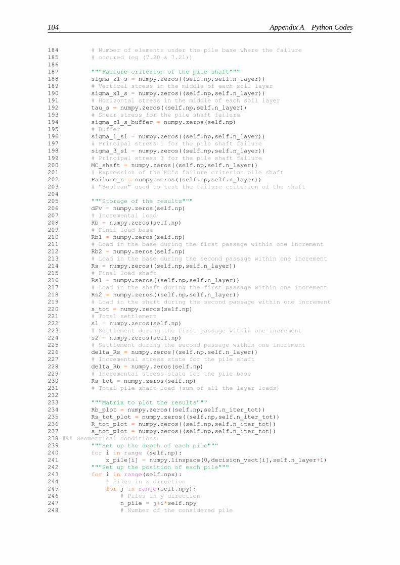
104 Appendix A Python Codes
184 # Number of elements under the pile base where the failure
185 # occured (eq (7.20 & 7.21))
186
187 """Failure criterion of the pile shaft"""
188 sigma_z1_s = numpy.zeros((self.np,self.n_layer))
189 # Vertical stress in the middle of each soil layer
190 sigma_x1_s = numpy.zeros((self.np,self.n_layer))
191 # Horizontal stress in the middle of each soil layer
192 tau_s = numpy.zeros((self.np,self.n_layer))
193 # Shear stress for the pile shaft failure
194 sigma_z1_s_buffer = numpy.zeros(self.np)
195 # Buffer
196 sigma_1_s1 = numpy.zeros((self.np,self.n_layer))
197 # Principal stress 1 for the pile shaft failure
198 sigma_3_s1 = numpy.zeros((self.np,self.n_layer))
199 # Principal stress 3 for the pile shaft failure
200 MC_shaft = numpy.zeros((self.np,self.n_layer))
201 # Expression of the MC's failure criterion pile shaft
202 Failure_s = numpy.zeros((self.np,self.n_layer))
203 # "Boolean" used to test the failure criterion of the shaft
204
205 """Storage of the results"""
206 dFv = numpy.zeros(self.np)
207 # Incremental load
208 Rb = numpy.zeros(self.np)
209 # Final load base
210 Rb1 = numpy.zeros(self.np)
211 # Load in the base during the first passage within one increment
212 Rb2 = numpy.zeros(self.np)
213 # Load in the base during the second passage within one increment
214 Rs = numpy.zeros((self.np,self.n_layer))
215 # Final load shaft
216 Rs1 = numpy.zeros((self.np,self.n_layer))
217 # Load in the shaft during the first passage within one increment
218 Rs2 = numpy.zeros((self.np,self.n_layer))
219 # Load in the shaft during the second passage within one increment
220 s_tot = numpy.zeros(self.np)
221 # Total settlement
222 s1 = numpy.zeros(self.np)
223 # Settlement during the first passage within one increment
224 s2 = numpy.zeros(self.np)
225 # Settlement during the second passage within one increment
226 delta_Rs = numpy.zeros((self.np,self.n_layer))
227 # Incremental stress state for the pile shaft
228 delta_Rb = numpy.zeros(self.np)
229 # Incremental stress state for the pile base
230 Rs_tot = numpy.zeros(self.np)
231 # Total pile shaft load (sum of all the layer loads)
232
233 """Matrix to plot the results"""
234 Rb_plot = numpy.zeros((self.np,self.n_iter_tot))
235 Rs_tot_plot = numpy.zeros((self.np,self.n_iter_tot))
236 R_tot_plot = numpy.zeros((self.np,self.n_iter_tot))
237 s_tot_plot = numpy.zeros((self.np,self.n_iter_tot))
238 #%% Geometrical conditions
239 """Set up the depth of each pile"""
240 for i in range (self.np):
241 z_pile[i] = numpy.linspace(0,decision_vect[i],self.n_layer+1)
242 """Set up the position of each pile"""
243 for i in range(self.npx):
244 # Piles in x direction
245 for j in range(self.npy):
246 # Piles in y direction
247 n_pile = j+i*self.npy
248 # Number of the considered pile

A.1 Analytical calculation of a pile group 105
249 x[n_pile] = x[0]+i*decision_vect[self.np+1]
250 # x coordinate of the considered pile
251 y[n_pile] = y[0]+j*decision_vect[self.np+2]
252 # y coordinate of the considered pile
253 """Set up a distance matrix of the piles"""
254 for i in range(self.np):
255 for j in range(self.np):
256 if i==j:
257 r[i,j]=decision_vect[self.np]
258 else:
259 r[i,j]=numpy.sqrt((x[i]-x[j])**2+(y[i]-y[j])**2)
260 """Set up the influence radius for each pile"""
261 # Initiates instances of the class RadiusOfInfluence [m]
262 # From Lutz (2003), Tabelle 7.1
263 for i in range(self.np):
264 rm[i] = InfluenceRadius.lutz_alpha(
265 self, decision_vect[i], numpy.mean(self.nu), 2.5)
266
267 #%% Calculate vertical and horizontal stresses in the middle of each soil layer
268 for i in range(self.np):
269 for k in range(self.n_layer):
270 sigma_z1_s[i,k] = sigma_z1_s_buffer[i]+(0.5*
271 (z_pile[i,k+1]-z_pile[i,k]))*self.gamma[k]
272 sigma_z1_s_buffer[i] = sigma_z1_s_buffer[i]+(z_pile[i,k+1]-
273 z_pile[i,k])*self.gamma[k]
274 # Stock the value at the extremity of each layer to calculate
275 # the next stress state in the next middle layer
276 sigma_x1_s[i,k] = sigma_z1_s[i,k]*self.K0[k]
277 sigma_z0_pile[i] = sigma_z1_s_buffer[i]
278 sigma_z1_s_buffer[i] = 0
279 fsigma_z0_pile[i] = sigma_z0_pile[i]+decision_vect[
280 self.np]*self.gamma[self.n_bottom-1]
281 fsigma_x0_pile[i] = fsigma_z0_pile[i]*self.K0[self.n_bottom-1]
282
283 #%% Calculate the stiffness modulus of soil Es
284 for i in range(self.np):
285 for k in range(self.n_layer):
286 Es[k] = self.ve*self.sigma_ref*(sigma_z1_s[i,k]/
287 self.sigma_ref)**self.we
288
289 #%% Calculate coefficient of influence from pile shaft j on pile shaft i (7.6)
290 # "Einflussbeiwert des Pfahlmantelwiderstandsanteiles"
291 # Here i and j indexes don't stick to x and y axes, each pile within
292 # the radius of influence is taken into account one after another
293 for k in range(self.n_layer): # For each layer
294 for i in range(self.np):
295 for j in range(self.np):
296 fs[i,j,k] = (1+self.nu[k])/(Es[k]*numpy.pi*
297 (z_pile[i,k+1]-z_pile[i,k]))*numpy.log(rm[i]/r[i,j])
298 # NB: log coresponds to the neperian logarithmus
299 if r[i,j] > rm[i]:
300 fs[i,j,k] = 0
301 # The coefficient is set to 0 if the radius of
302 # influence is exceeded
303
304 #%% Calculate the coefficient of influence from base j on base i (eq 7.7)
305 # 'Einflussbeiwert des Pfahlfußlwiderstandsanteiles'
306 for i in range(self.np):
307 for j in range (self.np):
308 fb[i,j] = (1-self.nu[self.n_layer]**2) /(Es[self.n_layer-1]*
309 numpy.pi*r[i,j])
310 if i == j:
311 fb[i,j] = fb[i,j] * numpy.pi/2
312 #%% Assemble matrix a (equation 7.15)
313 for k in range (self.n_layer):

106 Appendix A Python Codes
314 for i in range (self.np):
315 for j in range (self.np):
316 a[i+self.np*k,j+self.np*k] = fs[i,j,k]
317 for i in range (self.np):
318 for j in range (self.np):
319 a[i+self.np*self.n_layer,j+self.np*self.n_layer] = fb[i,j]
320 for i in range ((self.n_layer+1)*self.np):
321 a[(self.n_layer+1)*self.np,i] = 1
322 a[i,(self.n_layer+1)*self.np] = -1
323
324 #%% Assemble vector c (equation 7.15)
325 c[(self.n_layer+1)*self.np] = 1 # equivalent to c[-1] = 1
326
327 #%% Calculation procedure (see "7.3 Eigenes analytisches Berechnungsverfahren")
328 for iteration in range(self.n_iter_tot):
329 # Beginning of the loop
330 for i in range(self.np):
331 dFv[i] = self.Fv[i]/self.n_iter_tot
332 # Calculate the value of the additional force for each increment
333 laufwhile = 1
334 lauf1 = 0
335 while laufwhile != 0:
336 # The loop runs until two succesive values of Rb, Rs or s don't
337 # differ of more than 1%
338 lauf1 += 1
339 if lauf1 > 100:
340 print('Divergence')
341 break
342
343 #%% Resolution of the equation of equilibrium (1st time)
344 db = numpy.linalg.solve(a,c) #a*x=c solved by linalg.solve(a,c)
345 # db contains delta_Rs from line 1 to np*n_layer, delta_Rb from
346 # line np*n_layer to np*(n_layer+1), ds line 1+np*(n_layer+1),
347 # cf. equation (7.15)
348 for i in range(self.np):
349 delta_Rb[i] = db[self.n_layer*self.np+i]*dFv[i]
350 # eq (7.13b), calculation of the incremental stress state
351 # for the pile base
352 Rb1[i] = Rb[i]+delta_Rb[i]
353 for k in range (self.n_layer):
354 for i in range(self.np):
355 delta_Rs[i,k] = db[k*self.np+i]*dFv[i] # eq (7.13c),
356 # calculation of the stress state for the pile shaft
357 Rs1[i,k] = Rs[i,k]+delta_Rs[i,k]
358
359 #%% Determination of the failure criterion for the base
360 for i in range(self.np):
361 fc[i] = decision_vect[i]
362 # Depth node j (unit load applied)
363 fz[i] = decision_vect[i]+decision_vect[self.np]
364 # Depth node i (where displacement evaluated)
365 for i in range(self.np):
366 n_failure_b[i] = 0
367 for f in range (self.f_iter):
368 fx[f] = f*2/9*2*decision_vect[self.np]
369 # Source unknown
370 fr[f] = (fx[f]**2+fy**2)**0.5
371 # fy was set to 0
372 fR1[i,f] = (fr[f]**2+(fz[i]-fc[i])**2)**0.5
373 # cf CHOW, eq (15), (1986)
374 fR2[i,f] = (fr[f]**2+(fz[i]+fc[i])**2)**0.5
375 fsigma_x[i,f] = fsigma_x0_pile[i]-
Rb1[i]/(8*numpy.pi*(1-self.nu[self.n_bottom-1]))*((1-2*self.nu[self.n_bottom-
1])*(fz[i]-fc[i])/(fR1[i,f]**3)-3*fx[f]**2*(fz[i]-fc[i])/(fR1[i,f]**5)+(1-
2*self.nu[self.n_bottom-1])*(3*(fz[i]-fc[i])-4*self.nu[self.n_bottom-

A.1 Analytical calculation of a pile group 107
1]*(fz[i]+fc[i]))/(fR2[i,f]**3)-(3*(3-4*self.nu[self.n_bottom-1])*fx[f]**2*(fz[i]-
fc[i])-6*fc[i]*(fz[i]+fc[i])*((1-2*self.nu[self.n_bottom-1])*fz[i]-
2*self.nu[self.n_bottom-1]*fc[i]))/(fR2[i,f]**5)-
30*fc[i]*fx[f]**2*fz[i]*(fz[i]+fc[i])/(fR2[i,f]**7)-4*(1-self.nu[self.n_bottom-
1])*(1-2*self.nu[self.n_bottom-1])/fR2[i,f]/(fR2[i,f]+fz[i]+fc[i])*(1-
fx[f]**2/(fR2[i,f]*(fR2[i,f]+fz[i]+fc[i]))-fx[f]**2/fR2[i,f]**2))
376 fsigma_z[i,f] = fsigma_z0_pile[i]-
Rb1[i]/(8*numpy.pi*(1-self.nu[self.n_bottom-1]))*(-(1-2*self.nu[self.n_bottom-
1])*(fz[i]-fc[i])/(fR1[i,f]**3)+(1-2*self.nu[self.n_bottom-1])*(fz[i]-
fc[i])/(fR2[i,f]**3)-3*(fz[i]-fc[i])**3/(fR1[i,f]**5)-(3*(3-
4*self.nu[self.n_bottom-1])*fz[i]*(fz[i]*fc[i])**2-3*fc[i]*(fz[i]+fc[i])*(5*fz[i]-
fc[i]))/(fR2[i,f]**5)-30*fc[i]*fz[i]*(fz[i]+fc[i])**3/(fR2[i,f]**7))
377 ftau_xz[i,f] = -Rb1[i]*fx[f]/(8*numpy.pi*(1-
self.nu[self.n_bottom-1]))*(-(1-2*self.nu[self.n_bottom-1])/(fR1[i,f]**3)+(1-
2*self.nu[self.n_bottom-1])/(fR2[i,f]**3)-3*(fz[i]-fc[i])**2/(fR1[i,f]**5)-(3*(3-
4*self.nu[self.n_bottom-1])*fz[i]*(fz[i]+fc[i])-
(3*fc[i]*(fz[i]+fc[i])))/(fR2[i,f]**5)-
30*fc[i]*fz[i]*(fz[i]+fc[i])**2/(fR2[i,f]**7))
378 fsigma_1[i,f] =
0.5*(fsigma_x[i,f]+fsigma_z[i,f])+((fsigma_x[i,f]-
fsigma_z[i,f])**2/4+ftau_xz[i,f]**2)**0.5
379 fsigma_3[i,f] = 0.5*(fsigma_x[i,f]+fsigma_z[i,f])-
((fsigma_x[i,f]-fsigma_z[i,f])**2/4+ftau_xz[i,f]**2)**0.5
380 # MC's fracture criterion for the pile base, eq (7.14)
381 MC_base[i,f] = 0.5*fsigma_1[i,f]*(1-numpy.sin(
382 self.phi[self.n_layer-1]*numpy.pi/180))-
0.5*fsigma_3[i,f]*(1+numpy.sin(self.phi[self.n_layer-1]*numpy.pi/180))-
self.cohes[self.n_layer-1]*numpy.cos(self.phi[self.n_layer-1]*numpy.pi/180)
383 if MC_base[i,f] > 0:
384 n_failure_b[i] += 1 # increment of 1
385 # If the failure criterion of the base is not fulfilled
386 # adapt matrix a AND solve again the equation b = a\c.
387 # If the failure criterion is fulfilled, don't adapt
388 # matrix a, verify directly the failure criterion for
389 # the shaft
390
391 #%% Update of the coefficient of influence from pile base j on pile base i
392 for i in range(self.np):
393 for j in range(self.np):
394 fb[i,j] = (1-self.nu[self.n_layer]**2)/(
395 Es[self.n_layer-1]*numpy.pi*r[i,j]
396 )*self.n_elem_b/(self.n_elem_b-n_failure_b[i]
397 +1e-10)
398 # equation (7.21)
399 if n_failure_b[i] == self.n_elem_b:
400 fb[i,j] = 0
401 # The failure occured, coefficient set to 0
402 elif i is j:
403 fb[i,j] = fb[i,j] * numpy.pi/2
404 #%% Adaptation of matrix a (first time) after the failure of the base, (7.16)
405 for i in range(self.np):
406 for j in range(self.np):
407 a[i+self.np*self.n_layer,
408 j+self.np*self.n_layer] = fb[i,j]
409 for i in range(self.np):
410 a[(self.n_layer+1)*self.np,i+self.np*self.n_layer] = 1
411 if n_failure_b[i] == self.n_elem_b:
412 a[self.n_layer*self.np+i,
413 (self.n_layer+1)*self.np] = 0
414 else:
415 a[self.n_layer*self.np+i,
416 (self.n_layer+1)*self.np] = -1
417
418 #%% Resolution of the equation of equilibrium (2nd time)
419 db = numpy.linalg.solve(a,c)

108 Appendix A Python Codes
420 # Solves a second time when failure criterion of the base
421 # not fulfilled (different solution due to the modification
422 # of matrix a)
423 for i in range(self.np):
424 s1[i] = db[(self.n_layer+1)*self.np]*dFv[i]
425 for i in range(self.np):
426 delta_Rb[i] = db[self.n_layer*self.np+i]*dFv[i]
427 Rb1[i] = Rb[i]+delta_Rb[i]
428 for k in range(self.n_layer):
429 for i in range(self.np):
430 delta_Rs[i,k] = db[k*self.np+i]*dFv[i]
431 Rs1[i,k] = Rs[i,k]+delta_Rs[i,k]
432
433 #%% Determination of the failure criterion for the shaft
434 for k in range(self.n_layer):
435 for i in range(self.np):
436 if Failure_s[i,k] == 0:
437 tau_s[i,k] = Rs1[i,k]/((z_pile[i,k+1]-
z_pile[i,k])*2*decision_vect[self.np]*numpy.pi)
438 sigma_1_s1[i,k] =
(sigma_z1_s[i,k]+sigma_x1_s[i,k])/2+((sigma_z1_s[i,k]-
sigma_x1_s[i,k])**2/4+tau_s[i,k]**2)**0.5
439 sigma_3_s1[i,k] =
(sigma_z1_s[i,k]+sigma_x1_s[i,k])/2-((sigma_z1_s[i,k]-
sigma_x1_s[i,k])**2/4+tau_s[i,k]**2)**0.5
440 # MC's failure criterion for the shaft (7.14)
441 MC_shaft[i,k] = 0.5*sigma_1_s1[i,k]*(1-
numpy.sin((self.phi[k]+self.psi[k])*numpy.pi/180))-
0.5*sigma_3_s1[i,k]*(1+numpy.sin((self.phi[k]+self.psi[k])*numpy.pi/180))-
self.cohes[k]*numpy.cos((self.phi[k]+self.psi[k])*numpy.pi/180)
442 if MC_shaft[i,k] >= 0:
443 Failure_s[i,k] = 1
444 #If the failure criterion of the shaft is not fulfilled,
445 # adapt another time the matrix a AND go back to the
446 # equation b = a\c "first time" If the failure criterion is
447 # fulfilled, go directly to the next iteration
448
449 #%% Update of the coefficient of influence from pile base j on pile base i
450 for k in range(self.n_layer):
451 for i in range(self.np):
452 if Failure_s[i,k] == 1:
453 for j in range(self.np):
454 if j is not i:
455 fs[i,j,k] = 0
456 # Coef set to 0 if failure appears
457 #%% Adaptation of matrix a (second time) after the failure of the shaft, (7.16)
458 for k in range(self.n_layer):
459 for i in range(self.np):
460 for j in range(self.np):
461 a[i+self.np*k,j+self.np*k] = fs[i,j,k]
462 for k in range(self.n_layer):
463 for i in range(self.np):
464 a[(self.n_layer+1)*self.np,
465 i+self.np*self.n_layer] = 1
466 if Failure_s[i,k] == 1:
467 a[k*self.np+i,(self.n_layer+1)*self.np] = 0
468 else:
469 a[k*self.np+i,(self.n_layer+1)*self.np] = -1
470
471 #%% Resolution of the equation of equilibirum (3rd resolution)
472 db = numpy.linalg.solve(a,c)
473 for i in range(self.np):
474 s2[i] = db[(self.n_layer+1)*self.np]*dFv[i]
475 # Second resolution
476 for i in range(self.np):

A.1 Analytical calculation of a pile group 109
477 delta_Rb[i] = db[self.n_layer*self.np+i]*dFv[i]
478 Rb2[i] = Rb[i]+delta_Rb[i]
479 for k in range(self.n_layer):
480 for i in range(self.np):
481 delta_Rs[i,k] = db[k*self.np+i]*dFv[i]
482 Rs2[i,k] = Rs[i,k]+delta_Rs[i,k]
483
484 #%% Verification of the iteration condition
485 # NB: the loop runs while boolean different from 0 (boolean is
486 # reset to 1 each time before entering the loop "while").
487 laufwhile = 0
488 # Set to 0, if difference < 1%, go out of the loop while
489 for i in range(self.np):
490 if abs((s2[i]-s1[i])/s2[i]) >= 0.01:
491 laufwhile = 1
492 for i in range(self.np):
493 if ((Rb2[i]-Rb[i])-(Rb1[i]-Rb[i]))/(Rb2[i]-Rb[i]) >= 0.01:
494 laufwhile += 1
495 for i in range(self.np):
496 for k in range(self.n_layer):
497 if ((Rs2[i,k]-Rs[i,k])-(Rs1[i,k]-
498 Rs[i,k]))/(Rs2[i,k]-Rs[i,k]+1e-10) >= 0.01:
499 laufwhile += 1
500 # End of the loop while
501
502 #%% Calculate total settlement, load shaft and load base
503 """Total settlement"""
504 for i in range(self.np):
505 s_tot[i] = s_tot[i]+s2[i]
506 """Total load in the pile base"""
507 for i in range(self.np):
508 Rb[i] = Rb[i]+delta_Rb[i]
509 """Total load in each layer of the pile shaft"""
510 for k in range(self.n_layer):
511 for i in range(self.np):
512 Rs[i,k] = Rs[i,k]+delta_Rs[i,k]
513 """Sum of all the layer loads to obtain a single pile shaft load"""
514 for i in range(self.np):
515 Rs_tot[i] = 0
516 for k in range(self.n_layer):
517 Rs_tot[i] = Rs_tot[i]+Rs[i,k]
518 """Total load in a pile"""
519 R_tot = Rb+Rs_tot
520 #%% Storage of the results after each iteration
521 Rb_plot[:,iteration] = Rb
522 Rs_tot_plot[:,iteration] = Rs_tot
523 # for i in range(self.np):
524 # if Rs_tot_plot[i,iteration] < 0:
525 # Rs_tot_plot[i,iteration] = 0
526 R_tot_plot[:,iteration] = R_tot
527 s_tot_plot[:,iteration] = -s_tot*100
528 # End of the incremental loop, increase dFv for the next loop
529 #%% Plot results
530 if self.plot_fig:
531 for i in range(2,5):
532 plt.figure()
533 plt.plot(Rs_tot_plot[i,:],s_tot_plot[i,:], color='#4682B4',
534 linestyle=':', marker='.', label='Rs_%s'%(i+1))
535 plt.plot(Rb_plot[i,:],s_tot_plot[i,:],color='orange',
536 linestyle=':', marker='.', label ='Rb_%s'%(i+1))
537 plt.plot(R_tot_plot[i,:],s_tot_plot[i,:],color='#2F4F4F',
538 linestyle='--', marker='o', label ='Rtot_%s'%(i+1))
539 plt.title('Pile %d, D = %s m'
540 %(i+1, 2*decision_vect[self.np]))
541 plt.xlabel('Load (kN)')

110 Appendix A Python Codes
542 plt.ylabel('Settlement (cm)')
543 plt.grid()
544 plt.box('on')
545 plt.legend()
546 graph_name = 'Load-settlement curve pile %s'%(i+1)
547 plt.savefig(graph_name+'.png')
548 plt.show()
549
550 fig = plt.figure()
551 plt.plot(x,y,'o', color='#2F4F4F', markersize=12)
552 plt.title('Position of the piles, a/D = %.1f'
553 % (decision_vect[self.np+1]/(2*decision_vect[self.np])))
554 plt.xlabel('x (m)')
555 plt.ylabel('y (m)')
556 plt.grid()
557 plt.box('on')
558 position = fig.add_subplot(111)
559 for i in range(self.np):
560 position.annotate('%s'%(i+1), xy=(x[i], y[i]),
561 xytext=(x[i]+0.25, y[i]+0.06))
562 # Assignement of the numerotation to each point
563 graph_name = 'Position of the piles'
564 plt.savefig(graph_name+'.png')
565
566 fig = plt.figure()
567 plt.plot(x,y,'o', color='#2F4F4F', markersize=0)
568 plt.title('Distribution resistances (MN)\nand settlement (cm)')
569 plt.xlabel('x (m)')
570 plt.ylabel('y (m)')
571 plt.grid()
572
573 plt.box('on')
574 plt.ylim([-1, max(y)+1])
575 plt.xlim([-1.5, max(x)+1.5])
576 # plt.axis('equal')
577 subplot = fig.add_subplot(111)
578 for i in range(self.np):
579 subplot.annotate('%.1f'%(R_tot[i]/1000), xy=((x[i], y[i])),
580 xytext=(x[i]-0.3, y[i]-0.1))
581 subplot.annotate('%.1f'%(s_tot[i]*100), xy=((x[i], y[i])),
582 xytext=(x[i]-0.25, y[i]-0.9))
583 subplot.add_artist(matplotlib.patches.Circle((x[i], y[i]),
584 R_tot[i]/(2*numpy.mean(R_tot)), edgecolor =
585 '#2F4F4F', facecolor = 'none', linestyle='-'))
586 graph_name = 'Benchm KKP1, Resistance and settlement distribution'
587 plt.savefig(graph_name+'.png')
588
589 print("Settlement: %10.2f cm" %(numpy.mean(s_tot)*100))
590 # Round the float to 2 decimal places in a 10-place field
591 return(numpy.mean(s_tot))
592
593 class InfluenceRadius(object):
594 """ This class gathers functions calculating the radius of influence using
595 different empirical models:
596 - Cooke (1974)
597 - Wroth (1979)
598 - Lutz using the correction factor alpha (2003)
599 - Lutz using the thickness of the compressible layer (2003)
600 - Liu (1996)
601 For more information see M. Rudolf (2005) p. 75"""
602
603
604 def __init__(self, diameter = None , length = None, poisson = None,
605 alpha = None, thickness = None):
606 self.diameter = diameter

A.1 Analytical calculation of a pile group 111
607 self.length = length
608 self.poisson = poisson
609 self.alpha = alpha
610 self.thickness = thickness
611
612 def cooke(self, diameter):
613 """Radius of influence using Cook's formula with parameters:
614 - Diameter"""
615 radius = 10*diameter # [m]
616 return(radius)
617
618 def wroth(self, length, rg, poisson):
619 """Radius of influence using Wroth's formula (1979) with parameters:
620 - Length of the pile
621 - Radius rg of the circle having the same area as the pile group
622 rg = sqrt(a*b/pi) with a and b dimensions of the pile group
623 - Poisson's ratio"""
624 radius = 2.5*length*(1-poisson)+rg # [m]
625 return (radius)
626
627 def lutz_alpha(self, length, poisson, alpha):
628 """Calculation of the radius of influence using Lutz's formula relative
629 of the coefficient alpha (2003). Alpha is a factor correcting the
630 formula of Wroth (1979), comprised between 2.5 and 5.5. Parameters:
631 - Length of the pile
632 - Poisson's ratio
633 - Alpha coefficient
634 NB: For an infinitely extended half space, alpha = 5.5 and for
635 H/L = 2, alpha = 2.5"""
636 radius = alpha*length*(1-poisson) # [m]
637 return (radius)
638
639 def lutz_thickness(self, length, poisson, thickness):
640 """Calculation of the radius of influence using Lutz's formula relative
641 of the "thickness of the compressible layer"(2003). Parameters:
642 - Lengths of the pile
643 - Poisson's ratio
644 - Thickness of the compressible layer"""
645 radius = 1/(0.18182+0.43636*length/thickness)*(1-poisson)*length # [m]
646 return(radius)
647
648 def liu(self, diameter, poisson, length, thickness):
649 """Radius of influence using the formula of Liu (1996) with parameters:
650 - Diameter of the pile
651 - Poisson's ratio
652 - Length of the pile
653 - Thickness of the compressible layer"""
654 radius = diameter*1.1*(1-3.5*poisson**2.5)*(thickness/length)**0.68*(
655 length/diameter)**0.85 # [m]
656 return (radius)
657
658 if __name__ == '__main__':
659 instance_pile = PileGroup()

112 Appendix A Python Codes
A.2 Multi-optimisation of a pile group # -*- coding: utf-8 -*-
1 """
2 Created on Tue Feb 20 16:04:37 2018
3
4 @author: Corentin
5 """
6
7 import time # Used to calculate the computation time
8
9 import pygmo as pg # Optimisation library, Pagmo 2.7
10
11 import matplotlib.pyplot as plt
12
13 from PileGroup_calculation_15param import PileGroup
14 # Imports the class "PileGroup"
15
16 tmps_total_1 = time.time() # Starts the measurement of the computation time
17
18 class PileOptimPareto(object):
19 """ Defines a User Defined Problem (UDP) with 2 objectives
20 (volume of the piles and settlement of the pile group), unconstrained """
21
22 def __init__(self, dim = 15):
23 self.dim = dim
24 # Set up the dimension of the problem (ie decision vector's dimension)
25 self.instance_pile = PileGroup()
26 # Creates one instance of the imported class PileGroup, defines
27 # it as a local variable
28
29 def get_nobj(self):
30 """ Sets up the number of objectives of the problem"""
31 return(2)
32
33 def get_bounds(self):
34 """ Sets up the lower and upper boundaries of the decision vector
35 (here pile length and pile radius, in meters)"""
36 return([10, 10, 10, 10, 10, 10, 10, 10, 10, 10, 10, 10, 0.6, 1.5, 1.5],
37 [25, 25, 25, 25, 25, 25, 25, 25, 25, 25, 25, 25, 1, 6, 6])
38 # of the form ([lower boudaries], [upper boudaries])
39 # ie lp = [10, 25], rp = [0.6, 1], dx = [1.5, 6], dy = [1.5, 6]
40
41 def get_name(self):
42 """ Sets up the name of the problem"""
43 return ("PileOptimPareto")
44
45 def fitness(self, decision_vect):
46 """ Defines the objectives of the problem.
47 "decision_vect" is of dimension "dim" """
48 objective1 = self.instance_pile.volume(decision_vect)
49 # Volume of the piles (m3)
50 objective2 = self.instance_pile.settlement(decision_vect)
51 # Settlement of the pile group (m)
52 return (objective1, objective2)
53
54 if __name__ == '__main__':
55 instance_pileoptim = PileOptimPareto()
56
57 #%% Input
58 generations = 30
59 # Number of generations of the algorithm
60 popul = 72
61 # Number of individuals that will be evolved (NB: for the NSGA-2
62 # algotithm, a minimum of 5 and a multiple of 4 individuals is needed)

A.2 Multi-optimisation of a pile group 113
63 algo_name = "NSGA2"
64 #algo_name = "MOEAD"
65 # Only used to give information in the plot, not necessary to run the algorithm
66
67 #%% Instantiates a problem and evolves it
68 probl = pg.problem(PileOptimPareto(15))
69 # Instantiates a pygmo problem constructing it from the UDP
70
71 nsga2 = pg.algorithm(pg.nsga2(gen = generations))
72 # Instantiates a pygmo algortihm (here the algorithm is defined in a class of
73 # the pygmo library, but it is possible to code our own algorithm (User Defined
74 # Algorithm, UDA))
75
76 tmps_init_1 = time.time()
77 # Starts the measurement of the initialisation of the population
78 pop = pg.population(probl, popul)
79 # Initialises the population made of individuals bound to the problem (number
80 # of fitness evaluations rises to the number of the population)
81 tmps_init_2 = time.time() - tmps_init_1
82
83 f = pop.get_f()
84 # Gets the initial fitness vector
85 plt.scatter(f[:,0], f[:,1]*100, color = 'black', label = 'Initial population',
86 marker = '.')
87 # Plots the initial fitness vector (one column contains one objective)
88
89 tmps_evolve_1 = time.time()
90 # Starts the measurement of the evolution of the algorithm
91 pop = nsga2.evolve(pop)
92 # Runs the evolution (optimisation) of the algorithm
93 tmps_evolve_2 = time.time() - tmps_evolve_1
94
95 nb_fitness_eval = pop.problem.get_fevals()
96 # Gets the number of times the objectives are calculated
97 x = pop.get_x()
98 # Gets the evolved decision vectors
99 f = pop.get_f()
100 # # Gets the evolved fitness vector
101
102 #%% Visualisation
103 plt.scatter(f[:,0], f[:,1]*100, color = 'red', marker = 'v', label =
104 'Evolved population (Pareto front)\nFitness evaluations: %d'
105 %nb_fitness_eval)
106 plt.scatter(318.08, 3.0, color = 'blue', label = 'Reference solution')
107 plt.plot([318.08, 318.08], [0, 3.0], 'b--', lw = 1.5)
108 # vertical line between points [318.08,0] and [318.08,3.0]
109 plt.plot([0, 318.08], [3.0, 3.0], 'b--', lw = 1.5)
110 # Plots the evolved fitness vector (one column contains one objective)
111 plt.xlim([0, 800])
112 plt.ylim([0, 13])
113 plt.title('Benchmark CPR1 variant 2, 15 parameters \n algorithm %s, %s
generations, %s individuals' %(algo_name, generations, popul))
114 plt.xlabel('Volume of the piles ($m^{3}$)')
115 plt.ylabel('Settlement (cm)')
116 plt.grid()
117 plt.legend(loc = 1)
118 # Legend box fixed at the top right corner
119 plt.savefig('Benchmark KPP1 variant 2 15 parameters, algorithm %s, %s
generations, %s individuals.png' %(algo_name, generations, popul))
120 plt.show()
121
122 tmps_total_2 = time.time() - tmps_total_1
123 # Ends the measurement of the total computation time
124 print("Execution time, init population : %10.2f min" %(tmps_init_2/60))
125 print("Execution time, algorithm: %10.2f min" %(tmps_evolve_2/60))

114 Appendix A Python Codes
126 print("Execution time, total: %10.2f min" %(tmps_total_2/60))
127
128 #%% Saves data, just in case
129 with open('Data %s_%s_%s 15 param.txt'
130 %(algo_name, generations, popul),'w') as out_file:
131 # 'w' refers to 'write'
132 out_string = "Fitness \n"
133 out_string += str(f)
134 out_string += "\n"*2 + "Decision vector: \n"
135 out_string += str(x)
136 out_file.write(out_string)

Appendix B Global and partial safety concept
With the introduction of Eurocode 7 in 2005 and its partial safety concept, a new approach concerning
design in the geotechnics has been taking place. A single standard safety concept has been unified in
Europe. The global safety factor made use of a single safety factor to ensure a sufficient safety level.
The safety concept derived from Eurocode 7 (or its counterpart ÖNORM EN 1997-1 in Austria or DIN
EN 1997-1 in Germany) is established by means of a reduction of the resistance values and an increased
action calculated with different safety factors. It has to be said that other comparable codes (such as the
DIN 1054:2005-01 in Germany [14]) have been maintained and applied as long as they do not contradict
Eurocode 7 within a coexistence period. The old code DIN 1054:1976-11 [13] has no longer been
applicable since 2008.
Two different limit states have to be analysed: the ultimate limit state aims at assuring a sufficient load-
bearing capacity and at excluding any threat for humans, whereas the serviceability limit state guarantees
the long-term usability of the construction.
B.1 Global safety concept A construction is said to be safe according to the global safety concept if the characteristic resistance
(abbreviated 𝑅) and the characteristic stress or action (commonly abbreviated 𝑆) verify the following
equation involving the global security factor η
RS (B.1)
Note that the action effect is commonly called E. Only one parameter is used to take into account all the
different types of inherent imponderability of the geotechnical construction. This parameter depends on
the considered load case according to DIN 1054:1976 [13]. Some objections can thus be made to this
concept, as exposed by Adam (2016) [1]:
For a major part of the geotechnical designs (slippage, tipping, load-bearing capacity of piles…)
differentiated safety factors exist, determined empirically or arbitrarily.
Every design load cannot be evaluated separately, making the safety concept untraceable.
This concept is not able to depict the safety reserves or the utilisation factor of the construction.
That is why a new concept was developed that aims to eliminate these drawbacks.
B.2 Partial safety factor concept For every calculation step, the dispersion of the influence parameters is directly included using the so-
called partial safety factors γ. Resistances and stresses are described using characteristic values (index
k), representing the “safe” mean value of statistical analyses (that is to say somewhat more than the
mean value of the action respectively somewhat less than the mean value of the resistance). The
characteristic values are then increased or attenuated using partial safety factors, whether they operate
favourably or unfavourably (see equation (B.2) and Adam (2016) [1]). The obtained values are called
design values (index d).

116 Appendix B Global and partial safety concept
Ekd SS
R
kd
RR
(B.2)
The calculation of design values can be generalised. For actions, it is either directly determined or
derived from a representative value Frep that is multiplied by a partial factor γF (ÖNORM B 1997-1-1)
as in Equation (B.3).
Frepd FF (B.3)
For geotechnical parameters, they are calculated using the characteristic value divided by the partial
safety factor of the material γM.
M
kd
XX
(B.4)
Following ÖNORM B 1997-1-1 (the national guidance of Eurocode 7), all material safety factors γM
used to design pile foundations or shallow foundations are equal to 1. That is to say, all design
approaches in Austria are conducted using the characteristic soil parameters.
In Eurocode 7, three design approaches are presented. They depict the different calculation and design
philosophies existing in Europe [1]. In Austria, only the Design Approaches (DA) 2 and 3 are employed.
It is also stated that for pile and shallow foundations, the DA 2 has to be applied (ÖNORM B 1997-1-
1). For the DA 2, it should be verified that “a limit state of rupture or excessive deformation will not
occur using following combination of sets of partial factors” see [20]:
Combination: A1 “+" M1 "+" R2
The following terminology is adopted: A refers to the Actions, M to the Material properties and R to the
Resistances. In this approach, partial factors are applied to actions or to the effects of actions A
(equivalents of the German “Einwirkung” and “Beanspruchung”) and to ground resistances R. They do
not apply to material properties (all material safety factors are set to γM = 1 in the set M1). As an example,
the table of sets A1 and A2 is presented in Table B.1 (see Annex A.3 of Eurocode 7-1). Using the design
values outlined above, the two limit states can be verified.
Ultimate limit state
The ultimate limit state is verified if the design value of the action Sd is not exceeding the design value
of the resistance of a construction Rd or a construction part.
R
kddSk
RRSS
(B.5)

B.3 Comparison of the two concepts 117
Table B.1: Partial factors on actions following two different sets of partial factors [20].
Serviceability limit state
The design of the serviceability limit state is carried out by the equation
dd CE (B.6)
in which Cd represents the design value of the decisive serviceability criterion. For example, a
deformation serviceability criterion is the limit value of the deformation, after which the serviceability
of a structure is not given (for example not admissible cracks). This limit value has to be set during the
design of the structure.
B.3 Comparison of the two concepts Both concepts are summarised in Figure B.1. In particular, Eurocode 7 introduces new requirements
regarding the calculation of piles. Some characteristics of a pile group have to be designed more
precisely than it had been the case in DIN 1054:1976-11 [13], for example:
the group effect of a pile group,
the settlement differences between piles of a group and
the non-linear load-bearing behaviour.
Figure B.1: Representation of the global and partial safety concepts.


Appendix C Optimisation
C.1 Academic benchmark To study the influence of the input parameters on the efficiency of the algorithm, an academic
benchmark is carried out. The problem considered in this study, i.e. the first problem of the ZDT family
in two dimensions, was presented in Section 6.1.1 together with the associated metric used to quantify
the quality of the solution.
C.1.1 Influence of the number of generations
To optimise the ZDT1 problem, the number of individuals that are to be evolved for each simulation
must be determined. One then varies the number of generations applied to this initial population and
evaluates the precision of the obtained Pareto front. It is clear due to Figure C.1 that the higher the
number of generations, the greater the precision of the convergence. If the initial population is not
evaluated, selected, mutated and inserted in the new population a sufficient number of times, decision
vectors are not able to converge to an optimal Pareto set. For only two generations, the distance to the
Pareto front amounts to 2.45 but is reduced to 0.31 for 10 generations.
Figure C.1: Influence of the number of generations on the convergence of the genetic algorithm (a) 2
iterations (b) 4 iterations (c) 10 iterations.
(b)
(c)
(a)

120 Appendix C Optimisation
C.1.2 Influence of the population size
Here, the number of generations is fixed while the number of individuals is increased for each
simulation. It is noteworthy in Figure C.2 that the larger the population, the better the convergence. This
is due to mutations and crossovers, which occur for each iteration. Indeed, if the population is larger,
more individuals are mutated, creating a more diverse offspring. This offspring possibly contains
decision vectors closer to the analytical solution in comparison with a simulation featuring few
individuals. Mutation and crossover increase the chance to evolve to the optimal Pareto front. For 10
generations and 12 individuals, the distance to the Pareto front is 1.56, whereas when using 60
individuals, the optimal Pareto front is almost reached (distance of 0.03).
With a sufficient number of iterations and an adequate population size, the convergence to the optimal
Pareto front is reached (see Figure C.3).
It has to be added that some input parameters like the crossover rate can be optimal for one given
problem and unsatisfactory for another one. Some parameters are specific to each problem, but an
increasing number of generations or a larger initial population will unconditionally improve the quality
of the result. However, it leads to a more significant computational complexity.
Figure C.2: Influence of the population size on the convergence of the genetic algorithm (a) 12
individuals (b) 32 individuals (c) 60 individuals.
(a) (b)
(c)

C.2 Choice of the algorithm 121
Figure C.3: Convergence to the optimal Pareto front for 30 generations and 40 individuals.
C.2 Choice of the algorithm As mentioned in Section 6.1.3, different algorithms are implemented in pygmo and selectable by the
user. The algorithms MOEAD and NSGA-II were compared on the basis of the Benchmark “Guideline
1.2”.
The MOEAD algorithm turns out to be inapplicable for the present optimisation problem. In fact, the
algorithm tends to favour one objective over the other; it exaggerates the impact of the volume reduction
over the settlement objective, as pointed out in Figure C.4 (a) where only a part of the Pareto front is
covered. Decision vectors mainly stay in the area of minimum volumes with high settlements and do
not depict the whole range of optimal solutions.
Variations of the crossover and mutation rate as well as an increase of the number of generations and of
the population size did not result in forming an evenly distributed set of solution over the possibility of
the Pareto front in its entirety (see Figure C.4 (b)). Even if an improvement is to be attested, a lowest
settlement solution cannot be reached. The NSGA-II algorithm permits to cover a more significant range
of the optimal Pareto set as shown in Figure 6.4. This is why the NSGA-II is preferably chosen as a
basis for the present study. Nevertheless, not all algorithms are suitable for all problems, i.e. the
algorithm has to be chosen anew for each optimisation task.
Figure C.4: Application of the MOEAD algorithm on the benchmark “Guideline 1.2” (a) 15
generations, 48 individuals (b) 80 generations, 100 individuals.
(a) (b)