contribution of financial depth and financial access …
TRANSCRIPT
CONTRIBUTION OF FINANCIAL DEPTH AND FINANCIAL ACCESS TO POVERTY REDUCTION IN INDONESIA
Pinkan Mariskania Pasuhuk1
1 Regional Development Planning Agency (Bappeda), Yogyakarta Province, Indonesia. Email: [email protected]
This research attempts to analyze possible relationships between financial depth and financial access indicators with poverty in Indonesia. Financial depth indicators include the ratio of savings to gross domestic regional product and the ratio of credit to gross domestic regional product. Financial access indicators include the number of banks and number of cooperatives, while poverty is measured by poverty headcount ratio. This research utlizes a panel provincial level data in Indonesia consisting of 33 provinces for the period of 2007 to 2015. The main findings of this research is that financial development variables show a statistically significant negative relationship with poverty, confirming the contribution of financial depth and financial access in reducing poverty in Indonesia. However, the savings variable shows contradictory results, suggesting that in regions where the savings rate is high, the poverty rate tends to be high also. A possible explanation is that consumption of private and household sector contributes significantly to Indonesia’s GDP. Therefore, the effect of consumption is more effective in reducing poverty than the effect of savings.
Keywords : saving, credit, banking, cooperatives, poverty JEL Classification: E21, E51, G21, G28
ABSTRACT

Bulletin of Monetary Economics and Banking, Volume 21, Number 1, July 201896
2 The members of G20 countries are Argentina, Australia, Brazil, Canada, China, France, Germany, India, Indonesia, Italy, Japan, the Republic of Korea, Mexico, Russia, Saudi Arabia, South Africa, Turkey, the United Kingdom, the United States, and the European Union
3 The survey (Indonesia Family Life Survey or IFLS) was conducted in 13 provinces in Indonesia, which includes: North Sumatera, West Sumatera, South Sumatera, Lampung, DKI Jakarta, West Java, Central Java, DI Yogyakarta, East Java, Bali, West Nusa Tenggara, South Kalimantan, and South Sulawesi (Strauss et al., 2016)
I. INTRODUCTIONIndonesia has experienced a reduction in the poverty rate over the past 15 years. This has been achieved because of economic growth and multiple poverty alleviation programs, including social safety net program, conditional cash transfer program, expansion of credit to small and medium enterprises through KUR (Kredit Usaha Rakyat), and the community development program through PNPM (Program Nasional Pemberdayaan Masyarakat). The poverty headcount ratio has fallen to around half, from 19.14% in 2000 to 11.13% in 2015 (BPS, 2017). On the other hand, the financial sector in Indonesia is also growing to the objective of financial inclusion. The ownership of formal saving and credit account by adult population, for instance, shows an increasing trend. Financial sector development and financial inclusion have potentially become a new strategy for poverty alleviation.
In recent years, the focus of financial development issues has shifted to the provision of microfinance products for the middle-and-low-income population through the financial inclusion policy. The initiative for improving financial inclusion began in 2013 when the group of countries organized in the G202 committed to expanding access of formal financial services as one strategy for poverty alleviation by creating financial inclusion strategies in each country (Cull et al., 2014). The principle of financial inclusion is to ensure that everyone can receive financial services with the objective of increasing people’s income, so that those who are still living in poverty can get out of this situation by taking advantage of the financial services they receive.
The concept of financial inclusion is also encouraged by the existing financial sector that often excludes low-and-middle-income populations from its services. For example, to open a savings account in formal financial institutions, such as banks, requires a minimum deposit that is in many instances difficult for poor people to have. In addition, to obtain credit from banks, the banks require collateral in the form of assets, and often poor people do not have sufficient assets that can be used as collateral. This problem is considered a supply-side issue because it is related to the financial institutions as providers of services. However, the problem is not always from the supply side, as it can also come from the demand side. The presence of informal sources of finance, such as borrowing from friends and relatives, and also saving money in the form of assets (such as house, lands, jewelry), is also a reason why middle-and-low-income populations often do not access formal financial services.
In a household survey conducted in 20143, around 27% of the households surveyed had attempted to borrow money from sources other than families and

Contribution of Financial Depth and Financial Access to Poverty Reduction in Indonesia 97
friends. This number is insignificant compared to around 73% who did not borrow from other sources. For savings accounts, only 28% of households have them in formal financial institutions. In addition, 69% saved in the form of house and land, 71% owned vehicles, and 46% saved in the form of jewelry. The asset ownership of households is described in the figure 1.
0% 10% 20% 30% 40% 50% 60% 70% 80%
Vehicles
House and Land
Jewelry
Saving in Formal Financial Institutions
Source : author’s calculation, based on Strauss et al., “The Fifth Wave of The IndonesiaFamily Life Survey : Overview and Field Report”. March 2016
When households are identified based on poor and non-poor peoples, then the proportion of credit and savings account ownership can be observed in the figure 2.
Figure 1. Assets Owned by Households
Do notown
credit60%
Owncredit40%
Non-Poor HouseholdsCredit Ownership
Poor HouseholdsCredit Ownership
Do notown
credit88%
Owncredit12%

Bulletin of Monetary Economics and Banking, Volume 21, Number 1, July 201898
In the non-poor households, 40% of the households surveyed had credit at the time they were surveyed, and 60% of the households did not have any credit. In poor households, only 12% had credit while 88% did not have any credit from formal sources. For savings accounts, in non-poor households, 28% had savings, and 72% did not. By comparison, in poor households, 11% had savings accounts and 89% did not.
The figures illustrate how ownership of formal credit and savings accounts is very small in the group of poor households when compared to the non-poor households. As mentioned earlier, this condition might be caused by the supply side problem or demand side problem. However, the question to be addressed is whether or not the absence of formal credit and savings accounts in poor households is contributing to their poverty. Poor people are poor because either they do not access formal financial services or they do not access formal financial services because of their poor status.
Bhanerjee and Duflo (2011) argue that microcredit and saving access among poor people may help them escape poverty, although there are several problems with this. The impact of microcredit is very limited because its scope is usually small, and the activities are based on delivering small loans to poor people to build their businesses. However, the income effect of microcredit is incapable of lifting poor people out of their subsistence level. Although they are able to get out of the poverty trap, there is no further significant growth of their income (p.173). On the
Non-Poor HouseholdsSaving Ownership
Do notown
saving72%
Ownsaving
28%
Poor HouseholdsSaving Ownership
Do notown
saving89%
Ownsaving
11%
4 The classification of poor and non-poor households is based on 2014 poverty line in Indonesia for urban area, which is Rp.326,853 per capita per month, issued by Central Statistical Agency (BPS)
Source : author’s calculation, based on Strauss et al., “The Fifth Wave of The IndonesiaFamily Life Survey : Overview and Field Report”. March 2016
Figure 2. Ownership of Credit and Saving Account on Poor and Non-Poor Households4

Contribution of Financial Depth and Financial Access to Poverty Reduction in Indonesia 99
other hand, the saving activities of the poor may also be problematic. Similar to people from other income groups, poor people also face an uncertain future that creates a risk of shocks which will require them to draw down their reserves of assets in the future. Therefore, the importance of saving for the poor people is as high as people from other income groups, and they are also as capable as other people to save.5 However, the saving behavior of people is highly affected by their expectation of their future life, and the more they have a positive expectation, the greater is their savings. Psychologically, it is easier to make the decision to save money for the higher income groups than for the poor, because they have a more positive perception of their future and face less constraints on their expenditure. Therefore, the saving behavior of the poor is less consistent than that of high income people, which makes their prospects for the future worsen (p.191).
Financial sector can affect poverty at either the micro or macro level. At the micro level, household access towards microfinance products, such as savings and credits will potentially increase household’s income with several conditions, like consistent saving behavior and the usage of credit for business activities. In the macro level, the presence of financial institutions may encourage higher levels of saving in a country, which increases the money available for credit provision to business sectors in the economy, and it will increase investment in new businesses. Therefore, investments create employment opportunities, which contribute to poverty reduction.
II. THEORYMany studies relate financial sector development with economic growth, while other studies relate it with poverty reduction. A study by Ahmed and Ansari (1998) on three South Asian countries (India, Pakistan, and Sri Lanka) finds that financial sector development, which is measured by the ratio of broad money over Gross Domestic Product (GDP) and the ratio of domestic credit over Gross Domestic Product (GDP), caused economic growth in these three countries. Another study by De Gregorio and Guidotti (1995) also find that financial development has a positive relationship with economic growth. De Gregorio and Guidotti (1995) used two different sets of data, which were a sample of 98 countries from 1960 to 1985, and another data set of 12 Latin American countries from 1950 to 1985. Results were mixed. The evidence from the first dataset showed a positive and significant relationship between credit to private sector and GDP, while in the second data set, the result was the opposite. De Gregorio and Guidotti (1995) argued that after the 1970s, many Latin American countries attempted to liberalize their financial markets. However, because proper government regulations were not in place, there was excessive lending by the private sector. It is argued that, as a result of a high proportion of credit to private sector, there was crisis.
A subsequent study by Arestis, Demetriades, and Luintel (2001) confirms the positive relationship between financial development and economic growth. They test the relationship in five developed countries (the United States, Japan, the
5 This condition applies for people who live in moderate poverty, not extreme poverty

Bulletin of Monetary Economics and Banking, Volume 21, Number 1, July 2018100
United Kingdom, Germany, and France) using time-series data from 1968 to 1998 (ranging differently for each country). Their study included proxies from stock markets in addition to banks to measure financial development. The parameters used for stock market development were market capitalization and stock price volatility. The findings are mixed across countries, although in general, financial development is proven to have a positive relationship with economic growth. However, the evidence shows that banking sectors have a larger contribution than the stock market.
Jalilian and Kirkpatrick (2002) study how financial sector development contributes to lowering poverty for a panel of 42 developed and developing countries. Jalilian and Kirkpatrick (2002) argue that the effect of financial development on poverty is achieved through economic growth. Therefore, the first model examining the linkage between finance and growth can be written as:
where g is the growth rate of GNP, α1 is the intercept, X’is a vector of explanatory variables that include financial indicators6, Z’ is a vector of other explanatory variables7, β1 and γ1 are parameters of the equation, and ε1 is the error term.
To measure the effect on poverty, Jalilian and Kirkpatrick used two models. The first model is as follows:
6 Variables used as proxy for financial indicators are Bank Deposit Money Assets (BDMA) over GDP and Net Foreign Assets (NFA) over GDP.
7 Other explanatory variables include education, trade openness, change in inflation rate, change in trade share, initial income per capita, change in manufacturing share, public spending, developing countries dummy, and interactive term (developing countries dummy multiplied by BDMA). The study suggested that developing countries benefited more from financial sector development than developed countries.
8 Explanatory variables used in the poverty regression are gini coefficient, inflation, public expenditure, initial income per capita, and developing countries dummy.
where γctp is per capita income of the poorest quintile of the population in
country c year t, yct is average per capita income of the overall population in country c year t, and Xict is other factors of average income of the poor8(variable i in country c year t), and γ1 and γi are parameters of the estimate.
The second model is as follows:
i =1,….m

Contribution of Financial Depth and Financial Access to Poverty Reduction in Indonesia 101
where gctp is the growth of per capita income of the poor, gct is growth of per
capita income of all population, ∆Xict is the change of value for each variable, namely change in Gini, change in inflation, and change in public expenditure, and γ1 and γi are parameters of the estimate.
The main findings of this study suggest that NFA has a higher effect on economic growth in the sample countries compared to BDMA as a financial development indicator. In addition, developing countries benefited more from financial development than developed countries in terms of economic growth. For the poverty regression analysis, growth of income of the poor is significantly affected by growth of overall population, the Gini index, and the inflation rate. However, Jalilian and Kirkpatrick did not test the direct linkage between financial sector development and poverty, because in their study, they argued that poverty reduction will be achieved through economic growth.
Another study by Honohan (2008) identifies the relationship between financial service access and poverty using cross-country data consisting of 162 countries, including both developed and developing countries. He captures the dimension of financial widening9 in addition to financial depth and tested its connection to poverty in those countries. The proxy for poverty is proportion of population living under $1 per day, while independent variables included in the test are private credit to GDP ratio (as a proxy for financial depth), the inflation rate, institutions, GNI per capita of the bottom 90% of the population, and share of top-10% of the highest income in the population. Variables that were proven to have significant effects on poverty were private credit to GDP ratio, financial access, and the income distribution variables. Financial access and depth showed a negative sign, which is consistent with the main hypothesis that financial sector development lowers poverty. The GNI per capita of the bottom 90% of the population had a negative sign, while the share of the top-10% of the highest income in the population had a positive sign10.
Next, a study by Quartey (2005) investigates the relationship between financial sector development and poverty reduction in Ghana. This study takes the savings rate as the main indicator for financial development, along with domestic credit to GDP ratio, ratio of M2 to GDP, and per capita consumption as poverty measures11. To test the relation, Quartey apply the Granger causality test and the Johansen Cointegration test to find if there is long-run cointegration between financial indicators and poverty reduction.
To test the existence of causality, the poverty variable was tested with each of the financial variables, financial variables were tested with each other, and
9 Honohan (2007) used percentage of adults who own saving or credit account in formal financial institutions.
10 However, when the access variable is included in the same regression test with the depth variable, the access is not proven to be significant. It is only significant when regressed separately with depth variable, showing that both dimensions may have correlation with each other, and needs to be put in different test.
11 Quartey (2005) used time-series data taken from World Development Indicators for Ghana from 1970-2001

Bulletin of Monetary Economics and Banking, Volume 21, Number 1, July 2018102
different direction of causation was applied in each of the tests, as shown in the figure below.
12 Variance decomposition is done to explain the determinants of shocks in each variable, how much it is explained by the variable itself and by other variables.
Domestic Creditto GDP
Gross DomesticSaving to GDP
M2 to GDP Gross DomesticSaving to GDP
Per capitaConsumption
Gross DomesticSaving to GDP
M2 to GDPDomestic Credit
to GDP
Per capitaConsumption
Gross DomesticSaving to GDP
Per capitaConsumption M2 to GDP
Source : Quartey (2005)
Figure 3. Direction of Causation between Variables
The result shows that there is a statistically significant causality between domestic credit over GDP to per capita consumption. Moreover, the Johansen cointegration test confirms a long-run cointegration between financial development variables and per capita consumption as a proxy for poverty.
To further check the relationship between financial indicators and poverty, Quartey also conducted a variance decomposition test12 and a vector error correction

Contribution of Financial Depth and Financial Access to Poverty Reduction in Indonesia 103
model13. From the variance decomposition test, it was found that fluctuations of gross domestic saving and private credit to GDP are mostly explained by fluctuations of its own variable, and fluctuations of per capita consumption are mostly explained by gross domestic saving to GDP. The result of the vector error correction model showed that the value of R2 is above 0.6 for each variable, which means that the value of the variable is also explained by the variable itself in the previous periods.
The main results were that an increase in credit to private sector has a positive effect on per capita consumption, the decrease in per capita consumption has a negative and significant effect in gross domestic saving to GDP, and an increase in credit to private sector leads to lower gross domestic saving to GDP ratio. In conclusion, this study also confirmed the contribution of financial sector development to poverty reduction. However, the effect of savings to poverty was insignificant. Quartey argues that financial intermediaries in Ghana are unable to channel the domestic resources from saving to pro-poor investments.
III. METHODOLOGY3.1. Estimation Method and Variables The method of estimation is a panel OLS (Ordinary Least Squares) with fixed and random effects estimator. The dependent variable is poverty headcount ratio (a proxy for poverty). Poverty headcount ratio is the proportion of population living below the poverty line. The independent variables to be included in the model consist of financial variables and control variables. The financial variables are: (1) ratio of savings to GDRP (Gross Domestic Regional Products), (2) ratio of private credit to GDRP (Gross Domestic Regional Products), (3) number of banks, and (4) number of cooperatives14. (1) and (2) proxy for financial depth while (3) and (4) proxy for financial access. The control variables are: average years of schooling, life expectancy rate, real income per capita, and the Gini index. The selection of control variables is motivated by the work of Balisacan et al. (2002).
3.2. Econometric Model The econometric model is as follows.
13 For the vector-error correction model, regression analysis is exercised by adding the lag-length to three years (t-3) to identify whether the value of each variable is also explained by the value of the variables in t-1, t-2, and t-3.
14 Cooperatives are included because it is a common source for financing for Indonesian population, and in the Indonesia Family Life Survey (IFLS) conducted in 2007, cooperatives had become the second most often accessed institution after banks in the search for loans

Bulletin of Monetary Economics and Banking, Volume 21, Number 1, July 2018104
The model takes all variables in natural logarithmic form, where (P)it is poverty headcount ratio in province i year t, (S)it is saving to GDRP ratio in province i year t, (C)it is credit to GDRP ratio in province i year t, (BO)it is the number of bank office in province i year t, (Co)it is the number of cooperatives in province i year t, (Sc)it is average years of schooling in province i year t, (L)it is life expectancy rate in province i year t, (I)it is real per capita income in province i year t, (gini)it is gini index in province i year t, and ԑit is error term.
3.3. Data The data used in this study is panel provincial-level data for Indonesia, and the main sources of the data are the Indonesian statistics issued by the Central Statistical Agency (BPS), Indonesian Banking Statistics issued by the Indonesian Central Bank, Bank Indonesia (BI), and the Financial Service Authority (OJK). For banking statistics, the data are obtained from three banking reports, namely, Statistik Perbankan Indonesia, Statistik Bank Perkreditan Rakyat, and Statistik Perbankan Syariah. Currently, Indonesia is divided into 34 provinces, but the youngest province, which is North Kalimantan, is officially separated from East Kalimantan and became an independent province in 2012, so it is impossible to obtain statistics before 2012. Therefore, this province is omitted from the analysis. The years included in the sample are 2007-2015 (nine years), which result in 297 observations (33 provinces, nine years).
IV. RESULT AND ANALYSIS4.1. Cross Correlation MatrixTo identify the presence of multicollinearity, cross correlation matrix is presented in Table 1.

Contribution of Financial Depth and Financial Access to Poverty Reduction in Indonesia 105
Tabl
e 1.
Cro
ss C
orre
latio
n M
atri
x15
Log
(Pov
erty
)Lo
g (S
avin
g)Lo
g (C
redi
t)Lo
g (B
ank
Offi
ce)
Log
(Coo
pera
tive)
Log
(Sch
ool)
Log
(Lif
e Ex
pect
ancy
)Lo
g (I
ncom
e)Lo
g (G
ini)
Log
(Pov
erty
)1
-0.2
2258
7-0
.289
494
-0.2
9009
8-0
.194
003
-0.4
8548
7-0
.408
460
-0.2
9976
70.
0608
61
Log
(Sav
ing)
-0.2
2258
71
0.73
0726
0.21
5870
0.09
7828
0.36
0861
0.16
3437
-0.1
4401
00.
0161
27
Log
(Cre
dit)
-0.2
8949
40.
7307
261
0.22
8804
0.13
4679
0.34
7373
0.11
2569
0.12
6949
0.19
0073
Log
(Ban
k O
ffice
)-0
.290
098
0.21
5870
0.22
8804
10.
8922
730.
1261
870.
5289
940.
1912
260.
2137
74
Log
(Coo
pera
tive)
-0.1
9400
30.
0978
280.
1346
790.
8922
731
0.12
1014
0.48
8863
0.12
8856
0.14
3347
Log
(Sch
ool)
-0.4
8548
70.
3608
610.
3473
730.
1261
870.
1210
141
0.46
7009
0.03
0730
-0.1
2175
3
Log
(Life
Exp
ecta
ncy)
-0.4
0846
00.
1634
370.
1125
690.
5289
940.
4888
630.
4670
091
0.13
3227
0.05
9646
Log
(Inco
me)
-0.2
9976
7-0
.144
010
0.12
6949
0.19
1226
0.12
8856
0.03
0730
0.13
3227
10.
5184
57
Log
(Gin
i)0.
0608
610.
0161
270.
1900
730.
2137
740.
1433
47-0
.121
753
0.05
9646
0.51
8457
1
15 M
ultic
ollin
eari
ty e
xist
bet
wee
n va
riab
les
log(
savi
ng)
and
log(
cred
it),
vari
able
s lo
g(ba
nk_o
ffice
) an
d lo
g(co
oper
ativ
e),
vari
able
s lo
g(in
com
e) a
nd lo
g(gi
ni).

Bulletin of Monetary Economics and Banking, Volume 21, Number 1, July 2018106
4.2. Panel Fixed and Random Effect MethodsThe fixed and random effect methods can be divided into the following: (1) two-way fixed effects (cross-section and period fixed effects), (2) two-way random effects (cross-section and period random), (3) one-way fixed effects (cross-section fixed and period random), and (4) one-way fixed effects (cross-section random and period fixed). Since there is a problem of multicollinearity, the variables with the high correlation are not included in the same regression16.
The two-way fixed effect regressions that includes variables without high correlation is presented in in Table 2.
Table 2.Two-Way Fixed Effect Regression
Dependent Variable : Log(Poverty)Regression 1
Coefficient t-statistic Prob.C 4.977085 4.598720 0.000007LOG(SAVING) 0.036005 1.567476 0.118263LOG(BANK_OFFICE) -0.014754 -0.703713 0.482264LOG(SCHOOL) -0.095721 -0.488208 0.625828LOG(LIFE_EXP) -0.625869 -2.469626 0.014191LOG(INCOME) 0.056350 1.177685 0.240038
R2 0.988989Regression 2
Coefficient t-statistic Prob.C 4.685784 4.460348 0.000012LOG(CREDIT) 0.036318 1.652293 0.099725LOG(BANK_OFFICE) -0.010597 -0.515525 0.606640LOG(SCHOOL) -0.061393 -0.310660 0.756317LOG(LIFE_EXP) -0.611565 -2.424822 0.016022LOG(INCOME) 0.074292 1.602176 0.110374
R2 0.989000Regression 3
Coefficient t-statistic Prob.C 5.380353 4.855324 0.000002LOG(SAVING) 0.034141 1.525457 0.128404LOG(COOPERATIVE) -0.052683 -1.641962 0.101850LOG(SCHOOL) -0.074082 -0.378437 0.705426LOG(LIFE_EXP) -0.653031 -2.587680 0.010225LOG(INCOME) 0.057269 1.202986 0.230115
R2 0.989084
16 Log(saving) is not regressed together with log(credit), log(bank_office) is not regressed together with log(cooperative), and log(income) is not regressed together with log(gini).

Contribution of Financial Depth and Financial Access to Poverty Reduction in Indonesia 107
Table 2.Two-Way Fixed Effect Regression (Continued)
Regression 4Coefficient t-statistic Prob.
C 5.365112 4.828170 0.000002LOG(SAVING) 0.037780 1.726048 0.085569LOG(COOPERATIVE) -0.046627 -1.429684 0.154051LOG(SCHOOL) 0.011000 0.059175 0.952860LOG(LIFE_EXP) -0.570515 -2.273282 0.023855LOG(GINI) 0.076208 1.084444 0.279209
R2 0.989072Regression 5
Coefficient t-statistic Prob.C 4.688512 4.458971 0.000012LOG(CREDIT) 0.035046 1.591486 0.112759LOG(BANK_OFFICE) -0.009621 -0.467610 0.640469LOG(SCHOOL) 0.054051 0.288192 0.773438LOG(LIFE_EXP) -0.500178 -2.013003 0.045182LOG(GINI) 0.101385 1.467360 0.143530
R2 0.988982Regression 6
Coefficient t-statistic Prob.C 5.055290 4.643275 0.000006LOG(CREDIT) 0.033965 1.552072 0.121905LOG(COOPERATIVE) -0.042702 -1.310351 0.191275LOG(SCHOOL) 0.069096 0.368801 0.712587LOG(LIFE_EXP) -0.529966 -2.132108 0.033969LOG(GINI) 0.086399 1.236154 0.217557
R2 0.989048Regression 7
Coefficient t-statistic Prob.C 5.009077 4.644228 0.000006LOG(SAVING) 0.039120 1.745471 0.082127LOG(BANK_OFFICE) -0.014629 -0.698225 0.485683LOG(SCHOOL) -0.006096 -0.032779 0.973877LOG(LIFE_EXP) -0.543752 -2.163195 0.031470LOG(GINI) 0.092061 1.325809 0.186108
R2 0.989005Regression 8
Coefficient t-statistic Prob.C 5.109032 4.718205 0.000004LOG(CREDIT) 0.034867 1.598034 0.111293LOG(COOPERATIVE) -0.049837 -1.555107 0.121181LOG(SCHOOL) -0.041240 -0.209097 0.834542LOG(LIFE_EXP) -0.641709 -2.551704 0.011313LOG(INCOME) 0.074378 1.610989 0.108439
R2 0.989094Note : The probability values in italic are significant

Bulletin of Monetary Economics and Banking, Volume 21, Number 1, July 2018108
The two-way random effect regression that includes variables without high correlation is presented in Table 3.
Table 3.Two-Way Random Effect Regression
Dependent Variable : Log(Poverty)Regression 1
Coefficient t-statistic Prob.C 9.610679 7.564166 0.000000LOG(SAVING) 0.127202 5.032007 0.000001LOG(BANK_OFFICE) -0.110075 -4.772397 0.000003LOG(SCHOOL) -0.949556 -5.002319 0.000001LOG(LIFE_EXP) -0.919633 -2.912164 0.003867LOG(INCOME) -0.074389 -13.918370 0.000000
R2 0.735138Regression 2
Coefficient t-statistic Prob.C 8.770860 6.624221 0.000000LOG(CREDIT) -0.009848 -0.373332 0.709173LOG(BANK_OFFICE) -0.100382 -4.145217 0.000045LOG(SCHOOL) -1.031981 -5.227768 0.000000LOG(LIFE_EXP) -0.714689 -2.179485 0.030097LOG(INCOME) -0.084949 -16.575498 0.000000
R2 0.735076Regression 3
Coefficient t-statistic Prob.C 10.403175 8.084162 0.000000LOG(SAVING) 0.110712 4.381711 0.000016LOG(COOPERATIVE) -0.169039 -4.764634 0.000003LOG(SCHOOL) -0.939678 -4.934352 0.000001LOG(LIFE_EXP) -0.919160 -2.910355 0.003889LOG(INCOME) -0.077964 -15.821789 0.000000
R2 0.735076Regression 4
Coefficient t-statistic Prob.C 13.058086 8.649498 0.000000LOG(SAVING) 0.182551 6.260395 0.000000LOG(COOPERATIVE) -0.343446 -8.962765 0.000000LOG(SCHOOL) -0.404582 -1.837256 0.067192LOG(LIFE_EXP) -1.787595 -4.863569 0.000002LOG(GINI) -0.713338 -9.430031 0.000000
R2 0.622528

Contribution of Financial Depth and Financial Access to Poverty Reduction in Indonesia 109
Table 3.Two-Way Random Effect Regression (Continued)
Regression 5Coefficient t-statistic Prob.
C 10.231259 6.266449 0.000000LOG(CREDIT) -0.029556 -0.906720 0.365305LOG(BANK_OFFICE) -0.236332 -8.831215 0.000000LOG(SCHOOL) -0.455893 -1.919027 0.055959LOG(LIFE_EXP) -1.543060 -3.865877 0.000137LOG(GINI) -0.742559 -8.841269 0.000000
R2 0.558994Regression 6
Coefficient t-statistic Prob.C 12.096062 7.494855 0.000000LOG(CREDIT) -0.050037 -1.582810 0.114551LOG(COOPERATIVE) -0.384650 -9.602006 0.000000LOG(SCHOOL) -0.395216 -1.690283 0.092045LOG(LIFE_EXP) -1.589457 -4.060663 0.000063LOG(GINI) -0.819104 -10.489369 0.000000
R2 0.575346Regression 7
Coefficient t-statistic Prob.C 11.384481 7.634336 0.000000LOG(SAVING) 0.212429 7.473380 0.000000LOG(BANK_OFFICE) -0.225422 -9.314997 0.000000LOG(SCHOOL) -0.434729 -1.998972 0.046541LOG(LIFE_EXP) -1.723831 -4.725298 0.000004LOG(GINI) -0.591146 -7.417032 0.000000
R2 0.628961Regression 8
Coefficient t-statistic Prob.C 9.676935 7.277058 0.000000LOG(CREDIT) -0.018617 -0.719196 0.472597LOG(COOPERATIVE) -0.177655 -4.857814 0.000002LOG(SCHOOL) -0.980652 -4.995624 0.000001LOG(LIFE_EXP) -0.739217 -2.276556 0.023539LOG(INCOME) -0.085061 -17.694716 0.000000
R2 0.718098Note : The probability values in italic are significant
Bulletin of Monetary Economics and Banking, Volume 21, Number 1, July 2018110
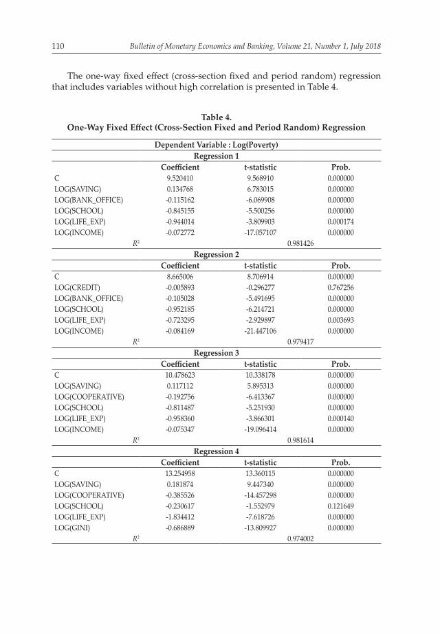
The one-way fixed effect (cross-section fixed and period random) regression that includes variables without high correlation is presented in Table 4.
Table 4.One-Way Fixed Effect (Cross-Section Fixed and Period Random) Regression
Dependent Variable : Log(Poverty)Regression 1
Coefficient t-statistic Prob.C 9.520410 9.568910 0.000000LOG(SAVING) 0.134768 6.783015 0.000000LOG(BANK_OFFICE) -0.115162 -6.069908 0.000000LOG(SCHOOL) -0.845155 -5.500256 0.000000LOG(LIFE_EXP) -0.944014 -3.809903 0.000174LOG(INCOME) -0.072772 -17.057107 0.000000
R2 0.981426Regression 2
Coefficient t-statistic Prob.C 8.665006 8.706914 0.000000LOG(CREDIT) -0.005893 -0.296277 0.767256LOG(BANK_OFFICE) -0.105028 -5.491695 0.000000LOG(SCHOOL) -0.952185 -6.214721 0.000000LOG(LIFE_EXP) -0.723295 -2.929897 0.003693LOG(INCOME) -0.084169 -21.447106 0.000000
R2 0.979417Regression 3
Coefficient t-statistic Prob.C 10.478623 10.338178 0.000000LOG(SAVING) 0.117112 5.895313 0.000000LOG(COOPERATIVE) -0.192756 -6.413367 0.000000LOG(SCHOOL) -0.811487 -5.251930 0.000000LOG(LIFE_EXP) -0.958360 -3.866301 0.000140LOG(INCOME) -0.075347 -19.096414 0.000000
R2 0.981614Regression 4
Coefficient t-statistic Prob.C 13.254958 13.360115 0.000000LOG(SAVING) 0.181874 9.447340 0.000000LOG(COOPERATIVE) -0.385526 -14.457298 0.000000LOG(SCHOOL) -0.230617 -1.552979 0.121649LOG(LIFE_EXP) -1.834412 -7.618726 0.000000LOG(GINI) -0.686889 -13.809927 0.000000
R2 0.974002
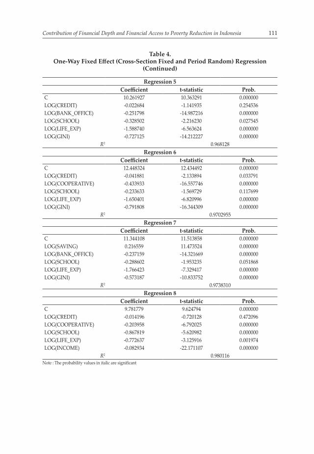
Contribution of Financial Depth and Financial Access to Poverty Reduction in Indonesia 111
Table 4. One-Way Fixed Effect (Cross-Section Fixed and Period Random) Regression
(Continued)
Regression 5Coefficient t-statistic Prob.
C 10.261927 10.363291 0.000000LOG(CREDIT) -0.022684 -1.141935 0.254536LOG(BANK_OFFICE) -0.251798 -14.987216 0.000000LOG(SCHOOL) -0.328502 -2.216230 0.027545LOG(LIFE_EXP) -1.588740 -6.563624 0.000000LOG(GINI) -0.727125 -14.212227 0.000000
R2 0.968128Regression 6
Coefficient t-statistic Prob.C 12.448324 12.434492 0.000000LOG(CREDIT) -0.041881 -2.133894 0.033791LOG(COOPERATIVE) -0.433933 -16.557746 0.000000LOG(SCHOOL) -0.233633 -1.569729 0.117699LOG(LIFE_EXP) -1.650401 -6.820996 0.000000LOG(GINI) -0.791808 -16.344309 0.000000
R2 0.9702955Regression 7
Coefficient t-statistic Prob.C 11.344108 11.513858 0.000000LOG(SAVING) 0.216559 11.473524 0.000000LOG(BANK_OFFICE) -0.237159 -14.321669 0.000000LOG(SCHOOL) -0.288602 -1.953235 0.051868LOG(LIFE_EXP) -1.766423 -7.329417 0.000000LOG(GINI) -0.573187 -10.833752 0.000000
R2 0.9738310Regression 8
Coefficient t-statistic Prob.C 9.781779 9.624794 0.000000LOG(CREDIT) -0.014196 -0.720128 0.472096LOG(COOPERATIVE) -0.203958 -6.792025 0.000000LOG(SCHOOL) -0.867819 -5.620982 0.000000LOG(LIFE_EXP) -0.772637 -3.125916 0.001974LOG(INCOME) -0.082934 -22.171107 0.000000
R2 0.980116Note : The probability values in italic are significant

Bulletin of Monetary Economics and Banking, Volume 21, Number 1, July 2018112
The one-way fixed effect (cross-section random and period fixed) regression that includes variables without high correlation is presented in Table 5.
Dependent Variable : Log(Poverty)Regression 1
Coefficient t-statistic Prob.C 5.654333 5.335876 0.000000LOG(SAVING) 0.032922 1.454623 0.146882LOG(BANK_OFFICE) -0.026251 -1.342705 0.180443LOG(SCHOOL) -0.313499 -1.693819 0.091400LOG(LIFE_EXP) -0.666495 -2.660473 0.008248LOG(INCOME) 0.055152 1.161403 0.246457
R2 0.824035Regression 2
Coefficient t-statistic Prob.C 5.377045 5.215721 0.000000LOG(CREDIT) 0.025498 1.178961 0.239404LOG(BANK_OFFICE) -0.022467 -1.168830 0.243456LOG(SCHOOL) -0.293972 -1.579563 0.115324LOG(LIFE_EXP) -0.647975 -2.595621 0.009935LOG(INCOME) 0.071647 1.553929 0.121319
R2 0.823636Regression 3
Coefficient t-statistic Prob.C 5.956207 5.509603 0.000000LOG(SAVING) 0.028473 1.283321 0.200430LOG(COOPERATIVE) -0.056719 -1.944375 0.052841LOG(SCHOOL) -0.293500 -1.581618 0.114854LOG(LIFE_EXP) -0.676397 -2.701056 0.007329LOG(INCOME) 0.056828 1.197185 0.232236
R2 0.825123Regression 4
Coefficient t-statistic Prob.C 5.960622 5.515136 0.000000LOG(SAVING) 0.031681 1.459532 0.145528LOG(COOPERATIVE) -0.051499 -1.745381 0.082004LOG(SCHOOL) -0.213492 -1.208204 0.227977LOG(LIFE_EXP) -0.593848 -2.390804 0.017465LOG(GINI) 0.083050 1.189141 0.235381
R2 0.825112
Table 5.One-Way Fixed Effect (Cross-Section Random and Period Fixed) Regression

Contribution of Financial Depth and Financial Access to Poverty Reduction in Indonesia 113
Table 5. One-Way Fixed Effect (Cross-Section Random and Period Fixed) Regression
(Continued)
Regression 5Coefficient t-statistic Prob.
C 5.391544 5.231849 0.000000LOG(CREDIT) 0.023875 1.102592 0.271141LOG(BANK_OFFICE) -0.021628 -1.125396 0.261375LOG(SCHOOL) -0.188413 -1.065479 0.287567LOG(LIFE_EXP) -0.538041 -2.191398 0.029238LOG(GINI) 0.108205 1.575574 0.116241
R2 0.823673Regression 6
Coefficient t-statistic Prob.C 5.699219 5.384193 0.000000LOG(CREDIT) 0.021745 1.007967 0.314331LOG(COOPERATIVE) -0.049020 -1.664050 0.097209LOG(SCHOOL) -0.175379 -0.989987 0.323026LOG(LIFE_EXP) -0.555098 -2.257334 0.024750LOG(GINI) 0.092093 1.326932 0.185601
R2 0.824499Regression 7
Coefficient t-statistic Prob.C 5.691065 5.389392 0.000000LOG(SAVING) 0.035505 1.604588 0.109700LOG(BANK_OFFICE) -0.026146 -1.337373 0.182175LOG(SCHOOL) -0.230194 -1.305979 0.192620LOG(LIFE_EXP) -0.583247 -2.348871 0.019518LOG(GINI) 0.098886 1.431645 0.153349
R2 0.824420Regression 8
Coefficient t-statistic Prob.C 5.726299 5.418324 0.000000LOG(CREDIT) 0.023011 1.067825 0.286509LOG(COOPERATIVE) -0.055025 -1.887649 0.060096LOG(SCHOOL) -0.275502 -1.477038 0.140777LOG(LIFE_EXP) -0.662704 -2.653526 0.008416LOG(INCOME) 0.071230 1.545159 0.123425
R2 0.824844Note : The probability values in italic are significant

Bulletin of Monetary Economics and Banking, Volume 21, Number 1, July 2018114
The regression results of the fixed and random effects can be summarized as follows:(1) Two-way fixed effects regression In the two-way fixed effects regression, none of the financial development
variables are statistically significant. The only variable that shows significance is log(life_exp).
(2) Two-way random effects regression In the two-way random effects regression, log(saving) is statistically significant
and positive, log(credit) is negative but statistically insignificant, log(bank_office) and log(cooperative) are statistically significant and negative, and all control variables are statistically significant and negative.
(3) One-way fixed effects (cross-section fixed and period random) regression In the cross-section fixed and period random effects regression, log(saving)
is statistically significant and positive, log(credit) is statistically significant and negative, but did so only in 1 of the 4 tests, log(bank_office) and log(cooperative) are negative and statistically significant, and other control variables are negative and statistically significant as well.
(4) One-way fixed effects (period fixed and cross-section random) regression In the period fixed and cross-section random effects regression, none of the
financial development variables are proven to be statistically significant, and the only statistically significant variable is log(life_exp).The Hausman test is run to further check the more appropriate method. And
the result of the Hausman test is presented in Table 6.
Test Summary Chi-Sq. Statistic Chi-Sq. d.f. Prob.Cross-section Random 44.2782 8 0.00000Period Random 123.3007 8 0.00000
Table 6. Hausman Test Result
The result of the Hausman test is statistically significant for both cross-section random period fixed effects and cross-section fixed period random effects, so both methods are relatively better than others.
The financial sector development is mostly associated with the policies made by the central government, such as the policy of interest rate that will affect the saving and credit provision, and the regulation for banking sector or cooperatives that will affect the presence of banks and cooperatives in a certain province. So, the unique characteristics of each province, such as the policy made by its regional government, are unlikely to affect our estimation. Therefore, the cross-section fixed and period random effects estimation method is more appropriate than the cross-section random and period fixed effects approach.
4.3. Robustness CheckFrom the cross-section fixed and period random effects regression result shown in Table 4, the variable log(saving) shows a positive and statistically significant

Contribution of Financial Depth and Financial Access to Poverty Reduction in Indonesia 115
relation, log(credit) is negative and statistically significant, log(bank_office) and log(cooperative) are negative and statistically significant, and all the control variables included in the model, namely log(school), log(life_exp), log(income) and log(Gini), are negative and statistically significant. All the results are as expected, except for log(saving) which shows contradictory result. The positive sign reflects that a higher savings rate leads to a higher poverty rate. This result is consistent in almost all the regression tests regardless of methods used.
To further check the robustness of the result, the following two regressions are estimated: (1) Regression by Omitting Outlier Jakarta is considered an outlier because of extreme values. Therefore, Jakarta
is omitted from the regression model. The result is presented in Table 7.
Table 7.Regression by Omitting Outlier
Dependent Variable : Log(Poverty)Regression 1
Coefficient t-statistic Prob.C 14.954385 7.066222 0.000000LOG(SAVING) 0.106183 2.380114 0.018748LOG(BANK_OFFICE) 0.000206 0.006339 0.994952LOG(SCHOOL) -1.818947 -5.562298 0.000000LOG(LIFE_EXP) -1.895785 -3.868936 0.000172LOG(INCOME) -0.075986 -11.916260 0.000000
R2 0.977725Regression 2
Coefficient t-statistic Prob.C 14.721846 6.952053 0.000000LOG(CREDIT) -0.060521 -1.710022 0.089629LOG(BANK_OFFICE) 0.025478 0.791244 0.430232LOG(SCHOOL) -2.024970 -6.382255 0.000000LOG(LIFE_EXP) -1.811592 -3.705012 0.000311LOG(INCOME) -0.082175 -14.551405 0.000000
R2 0.977395Regression 3
Coefficient t-statistic Prob.C 15.336275 7.753837 0.000000LOG(SAVING) 0.099551 2.280420 0.024198LOG(COOPERATIVE) -0.236482 -4.488827 0.000016LOG(SCHOOL) -1.401275 -4.571069 0.000011LOG(LIFE_EXP) -1.768333 -3.762766 0.000252LOG(INCOME) -0.059518 -9.696596 0.000000
R2 0.980152

Bulletin of Monetary Economics and Banking, Volume 21, Number 1, July 2018116
Table 7.Regression by Omitting Outlier (Continued)
Regression 4Coefficient t-statistic Prob.
C 17.158440 8.605638 0.000000LOG(SAVING) 0.185602 4.399982 0.000022LOG(COOPERATIVE) -0.419191 -8.927071 0.000000LOG(SCHOOL) -0.682454 -2.297026 0.023204LOG(LIFE_EXP) -2.410108 -5.209248 0.000001LOG(GINI) -0.489806 -5.974366 0.000000
R2 0.973126Regression 5
Coefficient t-statistic Prob.C 12.139505 5.689331 0.000000LOG(CREDIT) -0.072617 -2.047958 0.042562LOG(BANK_OFFICE) -0.138149 -4.847215 0.000003LOG(SCHOOL) -0.885103 -2.891031 0.004497LOG(LIFE_EXP) -1.911685 -3.907617 0.000149LOG(GINI) -0.754846 -9.649279 0.000000
R2 0.963105Regression 6
Coefficient t-statistic Prob.C 16.323851 8.160409 0.000000LOG(CREDIT) -0.030858 -0.865387 0.388409LOG(COOPERATIVE) -0.445905 -9.385027 0.000000LOG(SCHOOL) -0.790793 -2.667496 0.008606LOG(LIFE_EXP) -2.193730 -4.756284 0.000005LOG(GINI) -0.566956 -7.077966 0.000000
R2 0.967220Regression 7
Coefficient t-statistic Prob.C 13.023177 6.094741 0.000000LOG(SAVING) 0.257894 6.207509 0.000000LOG(BANK_OFFICE) -0.154926 -5.553148 0.000000LOG(SCHOOL) -0.631744 -2.053154 0.042048LOG(LIFE_EXP) -2.085426 -4.256430 0.000039LOG(GINI) -0.608694 -7.413549 0.000000
R2 0.967241Regression 8
Coefficient t-statistic Prob.C 14.718147 7.425882 0.000000LOG(CREDIT) -0.025452 -0.714981 0.475893LOG(COOPERATIVE) -0.233022 -4.339037 0.000028LOG(SCHOOL) -1.512686 -4.992515 0.000002LOG(LIFE_EXP) -1.604337 -3.441185 0.000778LOG(INCOME) -0.063991 -11.061210 0.000000
R2 0.979587Note : The probability values in italic are significant

Contribution of Financial Depth and Financial Access to Poverty Reduction in Indonesia 117
(2) Regression by Dividing Western and Eastern Parts The western part of Indonesia includes the following provinces: Aceh, North
Sumatera, West Sumatera, Riau, Jambi, South Sumatera, Bengkulu, Lampung, Bangka-Belitung, Riau islands, West Java, Central Java, Yogyakarta, East Java, Banten, and Bali. The eastern part of Indonesia include the following provinces: West Nusa Tenggara, East Nusa Tenggara, West Kalimantan, Central Kalimantan, South Kalimantan, East Kalimantan, North Sulawesi, Central Sulawesi, South Sulawesi, Southeast Sulawesi, Gorontalo, West Sulawesi, Maluku, North Maluku, West Papua, and Papua. The result of western part regression is presented in Table 8.
Table 8.Western Part Regression Result
Dependent Variable : Log(Poverty)Regression 1
Coefficient t-statistic Prob.C 14.469917 7.280917 0.000000LOG(SAVING) 0.107672 2.636794 0.009449LOG(BANK_OFFICE) 0.001479 0.050140 0.960092LOG(SCHOOL) -1.765838 -5.839293 0.000000LOG(LIFE_EXP) -1.795871 -3.944739 0.000133LOG(INCOME) -0.078277 -13.035774 0.000000
R2 0.972449Regression 2
Coefficient t-statistic Prob.C 14.127201 7.112559 0.000000LOG(CREDIT) -0.059783 -1.854594 0.066049LOG(BANK_OFFICE) 0.026580 0.907628 0.365849LOG(SCHOOL) -1.962855 -6.651161 0.000000LOG(LIFE_EXP) -1.693550 -3.733492 0.000287LOG(INCOME) -0.084791 -15.993063 0.000000
R2 0.971984Regression 3
Coefficient t-statistic Prob.C 14.943711 8.020135 0.000000LOG(SAVING) 0.102639 2.567591 0.011438LOG(COOPERATIVE) -0.243885 -5.064545 0.000001LOG(SCHOOL) -1.344689 -4.754887 0.000005LOG(LIFE_EXP) -1.676596 -3.839734 0.000196LOG(INCOME) -0.060944 -10.408710 0.000000
R2 0.975845

Bulletin of Monetary Economics and Banking, Volume 21, Number 1, July 2018118
Table 8.Western Part Regression Result (Continued)
Regression 4Coefficient t-statistic Prob.
C 17.041731 9.066108 0.000000LOG(SAVING) 0.190377 4.954935 0.000002LOG(COOPERATIVE) -0.418245 -9.753296 0.000000LOG(SCHOOL) -0.697785 -2.503005 0.013626LOG(LIFE_EXP) -2.374063 -5.544440 0.000000LOG(GINI) -0.531837 -6.719357 0.000000
R2 0.967478Regression 5
Coefficient t-statistic Prob.C 11.965478 5.927207 0.000000LOG(CREDIT) -0.068806 -2.127501 0.035375LOG(BANK_OFFICE) -0.131663 -5.042745 0.000002LOG(SCHOOL) -0.887936 -3.067267 0.002657LOG(LIFE_EXP) -1.885710 -4.151199 0.000061LOG(GINI) -0.814346 -10.780522 0.000000
R2 0.953507Regression 6
Coefficient t-statistic Prob.C 16.073405 8.545934 0.000000LOG(CREDIT) -0.026303 -0.809502 0.419790LOG(COOPERATIVE) -0.448195 -10.346999 0.000000LOG(SCHOOL) -0.788979 -2.832397 0.005400LOG(LIFE_EXP) -2.135438 -5.009793 0.000002LOG(GINI) -0.616612 -7.963689 0.000000
R2 0.964314Regression 7
Coefficient t-statistic Prob.C 13.029276 6.437264 0.000000LOG(SAVING) 0.261701 6.920644 0.000000LOG(BANK_OFFICE) -0.146755 -5.741832 0.000000LOG(SCHOOL) -0.652820 -2.249427 0.026264LOG(LIFE_EXP) -2.085444 -4.581316 0.000011LOG(GINI) -0.661771 -8.380267 0.000000
R2 0.959248Regression 8
Coefficient t-statistic Prob.C 14.187699 7.629145 0.000000LOG(CREDIT) -0.024123 -0.744633 0.457914LOG(COOPERATIVE) -0.240126 -4.893466 0.000003LOG(SCHOOL) -1.446596 -5.160256 0.000001LOG(LIFE_EXP) -1.487872 -3.445312 0.000781LOG(INCOME) -0.065973 -12.019562 0.000000
R2 0.975045Note : The probability values in italic are significant

Contribution of Financial Depth and Financial Access to Poverty Reduction in Indonesia 119
The result of western part regression is presented in Table 5.
Table 9.Eastern Part Regression Result
Dependent Variable : Log(Poverty)Regression 1
Coefficient t-statistic Prob.C 9.823059 8.795537 0.000000LOG(SAVING) 0.115003 5.488121 0.000000LOG(BANK_OFFICE) -0.178919 -7.166147 0.000000LOG(SCHOOL) -0.697720 -4.108824 0.000072LOG(LIFE_EXP) -1.019249 -3.600154 0.000460LOG(INCOME) -0.076812 -13.092495 0.000000
R2 0.985229Regression 2
Coefficient t-statistic Prob.C 9.376369 8.331527 0.000000LOG(CREDIT) 0.021863 0.970046 0.333927LOG(BANK_OFFICE) -0.177573 -7.046816 0.000000LOG(SCHOOL) -0.774611 -4.561788 0.000012LOG(LIFE_EXP) -0.882750 -3.108375 0.002337LOG(INCOME) -0.089785 -16.691777 0.000000
R2 0.983202Regression 3
Coefficient t-statistic Prob.C 8.905722 8.001620 0.000000LOG(SAVING) 0.101424 4.823560 0.000004LOG(COOPERATIVE) -0.153501 -4.438369 0.000020LOG(SCHOOL) -0.802658 -4.679065 0.000007LOG(LIFE_EXP) -0.625496 -2.278306 0.024434LOG(INCOME) -0.092300 -17.805677 0.000000
R2 0.983030Regression 4
Coefficient t-statistic Prob.C 12.335323 11.301537 0.000000LOG(SAVING) 0.173007 8.560483 0.000000LOG(COOPERATIVE) -0.373600 -12.016525 0.000000LOG(SCHOOL) -0.196562 -1.196106 0.233956LOG(LIFE_EXP) -1.694958 -6.356338 0.000000LOG(GINI) -0.820360 -12.856541 0.000000
R2 0.972491

Bulletin of Monetary Economics and Banking, Volume 21, Number 1, July 2018120
Table 9.Eastern Part Regression Result (Continued)
Regression 5Coefficient t-statistic Prob.
C 12.473199 11.309838 0.000000LOG(CREDIT) 0.005959 0.264290 0.791998LOG(BANK_OFFICE) -0.351504 -16.498664 0.000000LOG(SCHOOL) -0.202866 -1.233319 0.219808LOG(LIFE_EXP) -2.075845 -7.637342 0.000000LOG(GINI) -0.705187 -10.637551 0.000000
R2 0.971711Regression 6
Coefficient t-statistic Prob.C 11.969259 10.861965 0.000000LOG(CREDIT) -0.052995 -2.394720 0.018142LOG(COOPERATIVE) -0.440941 -14.693165 0.000000LOG(SCHOOL) -0.207518 -1.256925 0.211162LOG(LIFE_EXP) -1.596321 -5.938434 0.000000LOG(GINI) -0.966215 -15.753953 0.000000
R2 0.967800Regression 7
Coefficient t-statistic Prob.C 12.668484 11.651669 0.000000LOG(SAVING) 0.186217 9.410186 0.000000LOG(BANK_OFFICE) -0.315810 -14.887856 0.000000LOG(SCHOOL) -0.200366 -1.227444 0.222000LOG(LIFE_EXP) -2.060620 -7.669979 0.000000LOG(GINI) -0.551372 -8.078290 0.000000
R2 0.977856Regression 8
Coefficient t-statistic Prob.C 8.525337 7.628825 0.000000LOG(CREDIT) -0.003380 -0.151402 0.879907LOG(COOPERATIVE) -0.168596 -4.892621 0.000003LOG(SCHOOL) -0.854477 -4.984121 0.000002LOG(LIFE_EXP) -0.500304 -1.821707 0.070929LOG(INCOME) -0.101829 -21.077047 0.000000
R2 0.981416Note : The probability values in italic are significant
4.4. Discussion The variable log(saving) is consistently positive and statistically significant in the two additional regression tests. This result implies that in regions where the savings rate is high, the poverty rate is also high.

Contribution of Financial Depth and Financial Access to Poverty Reduction in Indonesia 121
4.5. Cointegration TestThe Pedroni residual cointegration test is performed to check the long-run cointegration between financial depth variables, financial access variables, and poverty17. Table 10 reports the results.
Table 10.Pedroni Residual Cointegration Test18
17 The variables included in the cointegration test are log(saving), log(credit), log(bank_office), log(cooperatives), and log(poverty)
18 The null hypothesis of Pedroni Residual Cointegration Test is no cointegration. 4 of 7 statistics are significant (probability values under 0.05), so the null hypothesis can be rejected
Statistic Prob.
Panel v-Statistic -3.37025 0.99962
Panel rho-Statistic 4.42100 1.00000
Panel PP-Statistic -8.29658 0.00000
Panel ADF-Statistic -5.55226 0.00000
Group rho-Statistic 7.406284 1.00000
Group PP-Statistic -10.8245 0.00000
Group ADF-Statistic -5.03787 0.00000
V. CONCLUSIONThis research analyzes possible relationship between financial development variables and poverty and examines the contribution of financial development to lowering poverty in Indonesia. The variables of interest are the ratio of savings to gross domestic regional product, ratio of credit to gross domestic regional products, number of banks, number of cooperatives, and poverty headcount ratio as a proxy for poverty. In several regression tests, the presence of banks and cooperatives is proven to have statistically significant and negative association with poverty, confirming the importance of financial institutions and their role in alleviating poverty. In addition, the ratio of credit to gross domestic regional products is also found to have a statistically significant and negative relation to poverty, although this result is not robust because of the inconsistency in different regression tests. However, the ratio of savings to gross domestic regional product is found to have positive and statistically significant association with poverty, and this result is consistent in several regression tests, suggesting that in regions where the savings rate is high, the poverty rate is also high. The possible explanation for this is that consumption of private and household sector (over the period of our

Bulletin of Monetary Economics and Banking, Volume 21, Number 1, July 2018122
study) contributes significantly to Indonesia’s GDP, while the financial resources obtained from savings is not channeled to pro poor investment. Therefore, the effect of consumption is more effective in reducing poverty than the effect of saving.
REFERENCESAhmed, S.M. and Ansari, M.I. (1998). Financial Sector Development and Economic
Growth : The South-Asian Experience. Journal of Asian Economics, Vol.9, No.3, pp.503-517
Arestis, Philip; Demetriades, Panicos O. and Luintel, Kul B. (2001). Financial Development and Economic Growth : The Role of Stock Markets. Journal of Money, Credit and Banking, Vol.33, No.1
Banerjee, Abhijit V. and Duflo, Esther. (2011). Poor Economics : A Radical Rethinking of The Way To Fight Global Poverty. Public Affairs New York
Balisacan, Arsenio M.; Pernia, Ernesto M.; Asra, Abuzar. (2002). Revisiting Growth and Poverty Reduction in Indonesia: What Do Subnational Data Show?, ERD Working Paper Series, No. 25. Asian Development Bank
Cull, R., Ehrbeck, T. and Holle N. (2014). Financial Inclusion and Development : Recent Impact Evidence. Consultative Group to Assist the Poor (CGAP) Focus Note No.92, April 2014
Demirguc-Kunt, A., Klapper, L., Singer, D. and Van Oudheusden, P. (2015). The Global Findex Database 2014 : Measuring Financial Inclusion Around The World. Policy Research Working Paper 7255. World Bank
De Gregorio, J. and Guidotti, P.E. (1995).Financial Development and Economic Growth. World Development, Vol.23, No.3, pp.433-448
Global Financial Development Report. (2014). World BankHonohan, P. (2008). Cross-county Variation in Household Access to Financial
Services. Journal of Banking and Finance 32, pp.2493-2500Jalilian, H. and Kirkpatrick, C. (2002).Financial Development and Poverty
Reduction in Developing Countries. International Journal of Finance and Economics 7, pp.97-108
Quartey, P. (2005). Financial Sector Development, Savings Mobilization and Poverty Reduction in Ghana. United Nations University World Institute for Development Economic Research, Research Paper No.2005/71
Strauss, J., Witoelar, F., and Sikoki, B. (2016). The Fifth Wave of The Indonesia Family Life Survey : Overview and Field Report Volume 1. Working Research 1143-1/NIA/NICHD RAND Labor and Population
Yunus, Muhammad. (2007). Banker To The Poor : Micro-lending and The Battle Against World Poverty. Public Affairs New York