contractor - nasa steering effects and the effects of having the vehicle traverse obstacles while in...

* 1 - 4

N A S A C O N T R A C T O R REPORT

?

I !

1 i

NASA CR - 61040

(TH U) 1 - I1

(CODE)

(NASA CR O R TMX O R AD NUMBER) ICA~TEOORY) I

NASA CR - 61040

(TH U) 1 - I1

(CODE)

(NASA CR O R TMX O R AD NUMBER) ICA~TEOORY) I

APOLLO LOOISTIC SUPPORT SYSTEMS MOLAB STUDIES

INTERIM REPORT ON MISSION COMMAND AND CONTROL

Prepared under cont rac t No. NASS-11096 by

Arch W. Meagher and Robert J. Bonham

NORTHROP SPACE LABORATORES Space Systems Section 6035 Tedhnology Drive

Huntsville, Alabama

For

GPO PRICE $

OTS PRICE(S) $

Hard copy (HC) 9Md Microfiche (MF

NASA - GEORGE C. MARSHALL SPACE FLIGHT CENTER

Huntsville, Alabama January 8, 1965

https://ntrs.nasa.gov/search.jsp?R=19650010249 2018-06-17T15:11:36+00:00Z

I '

0

CR -6 1040 Task Order N-46 January 8, 1965

APOLLO LOGISTIC SUPPORT SYSTEMS

MOLAB STUDIES

INTERIM REPORT ON

NUSSION COMMAND AND CONTROL

BY

Arch W. Meagher Robert J. Bonham

Distribution of this report is provided in the interest of information exchange. Responsibility for the contents resides in the author or organization that prepared it.

Prepared by Northrop Space Laboratories under Contract NAS 8-11096

For

R-ASTR-A ASTRIONICS LABORATORY

I ( * I ,

NASA-GEORGE C. MARSHALL SPACE FLIGHT CENTER

i

,

PREFACE

This Technical Report was prepared by the Northrop Space Laborator ies (NSL), Huntsville,' Department, for the George C. Marshal l Space Flight Center under authorization of Task Orde r N-46, Contract NAS8-11096.

The NASA Technical Representative w a s Mr . John F. Pavlick of the MSFC Astrionics Laboratory (R-ASTR-A).

The work completed was a twenty-four m a n week effort ending on December 2 3 , 1964.

The data presented herein include equations of motion, computer programs, and analysis of a four-wheeled LSV in the pitch and rol l planes where such an analysis pertains to the stability of the suspension and steering systems. Also included a r e equations of motion and computer diagrams for a six-wheeled LSV and a general block diagram which will s e rve a s a basis for studying the control of LSV's.

This is an inter im report .

i .

TABLE O F CONTENTS

e

e

Summary

1.0 Introduction

2 .0 Part I - F o u r Wheel Vehicle

2.1 Roll P lane Analysis

2 .1 .1 Procedure

2 .1 .2 Resul ts

2 .1 .2 .1 Acke rrnan St e e r ing

2.1.2.2 Obstacle T r a v e r s e While in an Ackerman Turn

2 . 2 P i tch P lane Analysis

2 .2 .1 P rocedure

2.2.2 Resul ts

2 .2 .2 .1 Resonance Analysis

2 .2 .2 .2 Forcing Functions Applied Simultaneously to All Wheels

2 .2 .2 .3 S equenti a1 Bump s

2 . 3 Conclusions and Recommendations

3.0 Par t 11 - Six Wheel Articulated Vehicle

3 .1 Roll P l ane Analysis

3.2 P i tch P lane Analysis

Part 111- Pre l imina ry Study of LSV Steering Control 4 .0

5.0 Symbols

6.0 Appendices

iii

Page 1

2

3

4

4

4

4

- 3

6

6

7

7

7

7

9

5 1

52

52

59

62

65

Figure

LIST O F ILLUSTRATIONS

Tit le

1A

1B

1c

1D

1E

1 F

2

3A

3B

4A

4B

4 c

4D

4E

4 F

4G

4H

41

4J

4K

4L

4 Wheel LSV - Mathematical Model

4 Wheel L S V - Roll Plane Equations

4 Wheel LSV - Roll Plane Equations

4 Wheel LSV - Mathematical Model, Pi tch Plane, Level Te r ra in

4 Wheel LSV - Mathematical Model, Pi tch Plane, Vehicle on Slope

4 Wheel LSV - Pi tch Plane Equations

CG Displacement v s Speed

Ratio CG Displacement to Bump Height v s Bump Height

Max. CG Acceleration v s Bump Height

Max. Ratio CG Displacement to Bump Height v s Bump Height






Max. and Min. P i tch Angle v s Bump Height




Max. and Min. Pitcfi Angle v s Bump Height


iv

Page

10

i1

12

13

13

14

15

16

17

18

19

20

21

2 2

23

2 4

25

26

27

28

29

'i

Figure

4M

4N

4 0

4 P

5A

5B

5 c

5D

5E

5 F

5G

5H

51

6A

6B

6C

6D

6E

6 F

7A

7B

7 c

7D

LIST O F ILLUSTRATIONS (Cont. )

Tit le

Random Surface T r a v e r s e




Roll Angle v s Wheel Angle




Max. Roll Angle Accelerations vs Speed

Speed vs Wheel Angle

Speed v s Wheel Angle



Max. Roll Angle vs Speed




Max. Roll Angle v s Speed


LSV -6 Wheel -Articulated, Mathematical Model

LSV -6 Wheel -Articulated, Roll Equations

LSV-6 Wheel - Articulated, Roll Equations

LSV-6 Wheel - Articulated, Roll Equations

Page

30

31

32

33

34

35

36

37

38

39

40

41

42

4 3

4 4

45

46

47

48

53

54

55

56

V

Figure

LIST O F ILLUSTRATIONS (Cont. )

Tit le

7 E

7F

8

I

LSV-6 W h el - Articulated, Mathematical Model, Pi tch Plane

LSV-6 Wheel - Articulated, Pi tch Equations

Block Diagram for Study of LSV Steering

LIST O F TABLES

Comparison of the 4-Wheel Vehicle with Vehicles Tested Previously

Page

57

58

61

49

r

.

vi

SUMMARY

The Mission Command and Control Task Order for which this repor t is written covers an analysis continued f rom the previous LSV task o r d e r . Areas to be covered are:

(1) Vehicle Stability (Suspension sys tems and vehicle design limits)

(2) Vehicle Steering

( 3 ) Control Systems (Beginning definition of control sys tems charac te r i s t ic s )

This is an in te r im repor t to cover the work done up until the t ime the task t ime l imit was extended.

As a bas is for this task, the NASA Technical Representative furnished paramet r ic data for two LSV's . and the other was a six-wheel, two-module, spring -coupled, art iculated vehicle. With the exception of using specified constants and data, this '

f i r s t the pitch plane performance for selected perturbations and then the steering (Roll Plane performance). This portion of the task for the four-wheel vehicle has been completed and the resu l t s , along with the equations of motion and computer diagrams used, a r e shown in the text of the repor t . the stability studies for the six wheel vehicle also a r e shown in the text of the repor t . either vehicles.

One was a four-wheel vehicle

m task was performed s imilar ly to previous tasks in this a r e a by examining,

t

Equations of motion and computer diagrams for completing

Only study of Ackerman steering has been outlined for

As a prel iminary approach to the control sys tems study, a block diagram i s included in this report . at tempt in defining the basic control problem and i t s expansion in the final repor t will include t ransfer functions and studies of the major sys tems and their components.

It is intended a s a first

I

4

1 . 0 . INTRODUCTION

This r epor t is presented in three pa r t s . Part I contains the equations of motion, the mathematical model and the resu l t s of pitch and rol l plane studies for a four wheel Lunar Surface Vehicle (LSV). I1 contains the pitch and roll plane equations of motion for studying a s ix wheel art iculated LSV. pa rame te r s is studied. study of the LSV command and control sys t ems . final repor t w i l l be expanded to include t ransfer fun-:tions and individual sys tem component analysis.

Part

In both c a s e s a par t icular vehicle with specified Tart 111 contains a pre l iminary block-diagram

In the la t te r c a s e the

The purpose of the Part I and Part I1 studies is to es tabl ish the lunar surface stability of a given design and specified pa rame te r s . While it is impract ical to study completely the stability and performance of the LSV, it is the intent to establish critical stability a r e a s and to indicate limits in a r e a s that may need fur ther study.

The purpose of Part 111 of this r epor t is to present a pre l iminary approach to controls problem studies for the LSV. problem i s intr icate , depending on numerous t ime delays, power r e - gulation, surface conditions and types of equipment used. No attempt wi l l be made to determine the equipment types used---just to establish in a general way the c r i t i ca l a r e a s of operation and the functional f eas - ibility of some equipment.

The complete controls

2

.

8

0

,

PART 1

FOUR WHEEL VEHICLE

3

2.1 ROLL PLANE ANALYSIS

2.1.1 PROCEDURE

The four-wheel vehic l i was studied in the rol l plane for two conditions--Ackerman steering effects and the effects of having the vehicle t r ave r se obstacles while in an Ackerman turn. model used for studying the vehicle is shown in F igure 1A and the equations of motion used a r e shown in F igures 1B and 1C. used in the rol l plane were impulse-type distrubances, the effects of the pitch plane coupling a r e included in the simulation. In these studies each of the wheels (on one s ide of the vehicle) s t ruck an obstacle sequentially and the length of t ime elapsed between the striking of the front and r e a r wheels was cor re la ted with the vehicle speed. The forcing function for traversing obstacles was simulated with a half-sine wave. A r a m p w a s used for the forcing function where Ackerman steering was simulated, The derivation of this forcing function is developed in Figure B4 of Appendix B. (in the roll plane) was accomplished through the use of a fixed moment added to the quation (6) of F igure 1B. this moment is shown in Figure B3 of Appendix B. applicable as long a s l e s s than three of the four Vehicle wheels a r e off of the Lunar surface.

The mathematical

Since the perturbations

Finally, the simulation of the LSV’s operating on a slope

The development of the use of This simulation is

The inclusions of the IC in the equations of motion (F igure 1B) will be explained in Section 2.2.1.

The analog computer schematic used fo r the rol l plane studies is shown in (F igure B1) Appendix B, and the data a r e shown in F igure B2. terrain-level position ( Z The forcing functions were se? to zero when the vehicle wheel was off of the Lunar surface.

The forcing functions for obstacle t r a v e r s e were applied a t the Zkr, etc. ) for all rol l plane simulations. of’

2.1.2 RESULTS

2.1.2.1 Ackerman Steering

a

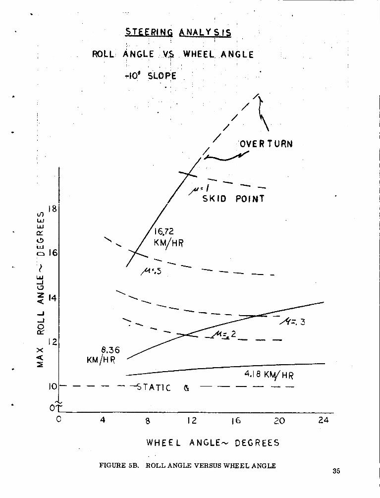
The resu l t s of the Ackerman s teer ing s tudies a r e shown in 8

Figure 5. slopes, a s indicated, with the yaw angle increasing negatively and the ro l l angle increasing negatively. ( o r to the r ight) while traveling forward (See F igure 1). obstacles were simulated in obtaining the resu l t s of Figure 5.

These studies were made with the vehicle on level t e r r a in o r

That i s , the vehicle was turned up the slope. No sur face *

Since the analog computer simulation assumed no skid condition for any of the tes t s , approximate skid l ines using the soil coefficient of friction and the moments c rea ted by the vehicle ro l l and yaw have been

4

calculated and added to the computer resu l t s . The skid point curves mean that the soil coefficient of friction had to be a s grea t a s that shown on the skid curve f o r a particular roll angle and wheel angle condition a t that point--or skidding occurred. vehicle yaw and rol l angles were reduced.

When skidding occur: ed both the

F igures 5A, 5B, 5C, and 5D w i l l show that the vehicle i s stable for the range of speeds (16.72 Km/hr is beyond the stated LSV design range), maximum wheel angles, and roll angle slopes indicated for the LSV. At the higher speeds, slopes and wheel angles the safzty margin seems small.

Angular accelerations (maximum) that occurred during the tes t s a r e shown on Figure 5E. formances a r e on f i le with R-ASTR-A Marshal l Space Flight Center .

T ime history t r aces of other pa rame te r s per -

2 .1 .2 .2 Obstacle T r a v e r s e While in an Ackerman Turn

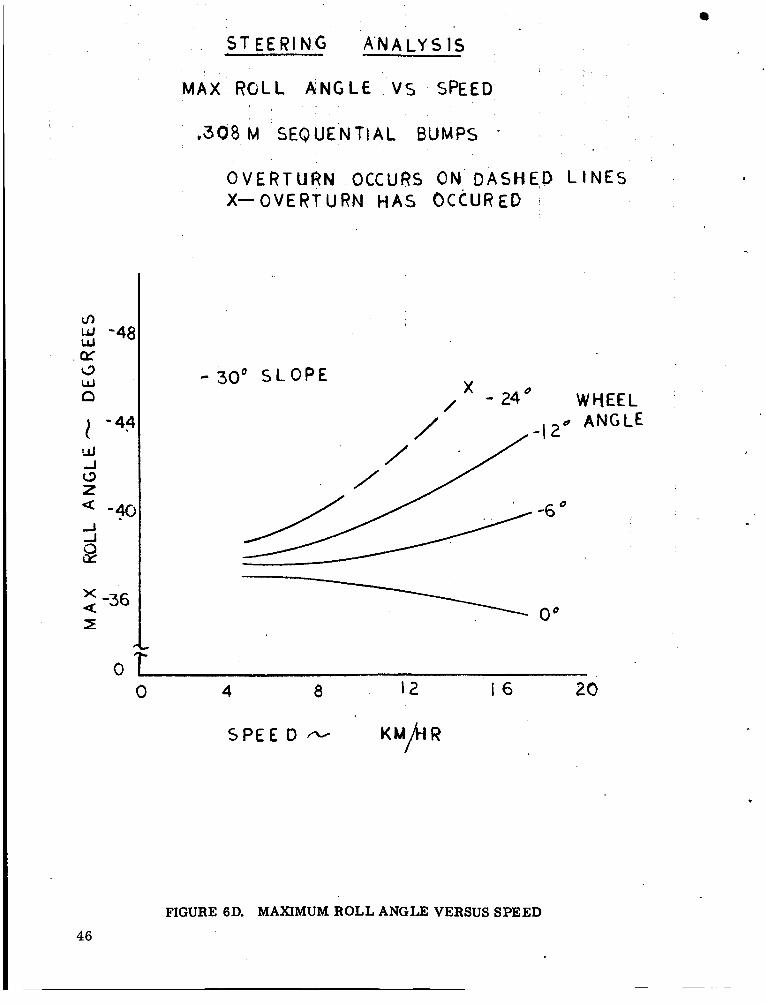
The conditions for testing the ability of the LSV to negotiate an obsta .de while making an Ackerman turn were t h e s a m e as those described in Section 2 . 2 . 2 . 1 , except in this case the wheel angle had already reached i t s maximum before the simulation (addition of perturbations) was s tar ted. This means that the r amp of equation (F igure 1B) 6 was se t a t the maximum value initially for a represented turning radius. added to the simulation by disturbing the wheels on the inside (up-hill) of the turn in a t imed sequence related to the vehicle speed. of these studies a r e shown in F igure 6. The maximum rol l angle of all the curves (ordinates) include the te r ra in slope.

The perturbations were

The resu l t s

The resu l t s indicate that for a l l slopes (including level t e r r a in ) the vehicle is unstable while making an Ackerman turn with a wheel of 24' and vehicle speeds of above 8Km/hr. As can be seen in F igures 6B, 6C, 6 ~ , 6E, and 6F, the veh ic l s w a s also either unstable o r marginally stable ( ro l l angles grea te r than 40 ) for smaller wheel angles, would b e eased somenhat if the vehicle had skidded. However, in studying the "worst case" it should b e remembered that there may be c a s e s where the vehicle cannot skid on level t e r r a in o r on slopes.

This situation

0

5

2 . 2 PITCH PLANE ANALYSIS

2.2.1 PROCEDURE

Where c a r e i s exercised in the choice of perturbations the stability character is t ics of a ra ther complicated vehicle can be studied in a r e - ' I

latively simple manner . four wheel vehicle shown in Figure 1.

This was the approach used in studying the

In studies to determine responses in the pitch plane step functions This simulates a Lunar ledge which is s t ruck f i r s t by the were used.

two front wheels and then, af ter a t ime delay (determined by the vehicle 's speed), by the r e a r wheels. neglected- -or not completely known--a quarter -sine wave function was used on the computer to simulate the s tep function. Such a function takes into consideration the t i r e iridentation and r e v e r s e thrust present when the vehicle s t r ikes a sha rp edged object. wave is a function of the speed of the vehicle.

Since t i r e indentation and r eve r se thrust was

The frequency oi the quarter-s ine

Pitch plane studies were made to determine resonance responses . In this case the forcing function was a continuous sine wave. The resonant response was determined by taking frequency increments and noting the amplitud 3s and amplitude build-up for a particular amplitude and frequency input. by use of the vehicle wheel-base. plane response to studies of other vehicles the modified s tep function described above was applied to a l l four vehicle wheels simultaneously. By varying the bump height of the obstacle t raversed , the nonlinear vehicular response to different speeds and bump heights is shown.

"

The speed of the vehicle was cor re la ted with the frequencies used In o r d e r to compare the vehicle pitch

I

Figures l D , l E , and 1 F show the mathematical models and the equations of motion for the pitch plane studies. w a s studied both for level t e r r a in and f o r the condition where the vehicle was going down slopes of 10 , 20 and 30 degrees . used for the la t ter study. equations. attached to l eve r s that extend to the r e a r of the main body. of the IC in the equations the vehicle was made to sett le (with no pe r tu r - bations) so that the r e a r wheel levers and the main body were paral le l to level te r ra in .

As is indicated, the vehicle

A body axis system was Note an initial condition (IC) indicated in the

This is used since the r e a r wheels of this vehicle a r e physically By the inclusion

The analog computer model used for the pitch plane studies is shown in Figure A1 of Appendix A, and the data a r e shown in F igure A2. The forcing functions were applied at the t e r r a i n level position ( 2 Z , e tc , ) for a l l pitch plane simulations. The forcing function became z::o when the vehicle wheel was off of the Lunar surface.

of'

6

2.2.2 RESULTS

2 . 2 . 2 . 1 Resonance Analysis

Resonance analysis resul ts of the four-wheel (using data of Appendix A) vehicle a r e shown in Figure 2. tude was low for this simulation, the vehicle did not leave the Lunar surface. between s ix and eight kilometers per hour.

t ies with the LSV stability.

Since forcing function ampli-

Under this operating condition the vehicle resonance occur s It should be noted that this

* is within the specified operating range of the vehicle and may cause difficul-

2 . 2 . 2 . 2 Forcing Functions Applied Simultaneously to All Wheels

F igure 3 shows f i e nonlinear vehicle response to different heights of obstacles t raversed . height and with the speed of the vehicle. discontinuity of the forcing function when the LSV leaves the Lunar s u r - f - - -

The nonlinearity va r i e s both with obstacle This i s pr imar i ly caused by the

d C e .

Figure ?A shows the peak displacement ( ra t ioed to the height 1 of the obstacle t r ave r sed ) of the vehicle center of gravity. The data

a r e self-explanatory and indicate the difficulty in keeping the LSV on the Lunar surface while it t r a v e r s e s surface obstacles . Both the displacement and the acceleration compare favorably with those of other vehicles

cases the perturbations caused overshoot, but in a l l ca ses the oscillations of the distrubance always settled in six to eight seconds. mos t of the studies on this vehicle a small amount of damping was in se r t - ed in the tires. It had very little effect , however, when compared to resul ts obtained under the same conditions-but with no t i r e damping. The t ime his tory t r aces of parameters such a s wheel displacement, acceleration, etc. , a r e on file at the Marshall Space Flight Center , R-ASTR-A.

v previously studied. This i s particularly t rue of the damping. In all

F o r this and

2 .2 .2 .3 Sequential Bumps

When the vehicle t raversed an object, such as a ledge, f i r s t the f ront wheels s t ruck and la te r , depending on the length of the wheel base and the vehicle speed, the r e a r wheels s t ruck the same ledge. sults of the four wheel LSV's traversing this type of obstacle is shown in F igure 4. were changed and the speed of the vehicle was changed. Figures 4A, 4B, 4C, and 4D show the resulting maximum displacement of the LSV center of gravity of under the tes t conditions. a r e shown for each condition- -the maximum CG displacement caused f rom the f ront wheel's striking and the maximum CG displacement f rom

The r e -

During these studies the height of the obstacles t r ave r sed *

In mos t cases two curves

7

the r e a r wheel's striking. dition indicates that the vehicle had s tar ted to set t le f rom the front wheel perturbation when the r e a r wheels struck. condition indicates that the peak of the CG displacement had not been reached when the r e a r wheel s t ruck. the curves a r e attributed both to the long wheel base and the method of attaching the r e a r wheels (on a l eve r ) to the main vehicle body. i s called to the difference in the general curve shapes for the 8.36 Km/hr conditions, This could be caused from the resonance descr ibed ea r l i e r . Fur ther examination would be required to make cer ta in . between Figure 3A and Figure 4A will demonstrate the effects of the high moment of iner t ia and the long wheel base given for this vehicle . of slopes on the vehicle's operation can be seen by comparing Figure 4A with Figures 4B, 4C and 4D.

The inclusion of two curves for a t e s t con-

One dashed curve for a t e s t

The somewhat percul iar shapes of

Attention

A comparison

Effects

CG accelerations under the t e s t conditions a r e shown in F igures Comparison of the upper curve of F igure 4E with those of 4E and 4F.

F igure 3B wi l l again point out the advantages of a high moment of iner t ia and a long wheelbase. Km/hr tes t condition a r e unique. is shown by the dash-line curve. wheels' striking a t other speeds were either l e s s than those caused by the front wheels o r they were identical to those of the front wheels, and a r e not shown.

Also the effects on the CG acceleration for the 8.36 The resu l t of the r e a r wheel's striking Accelerations to the CG f rom the r e a r

I

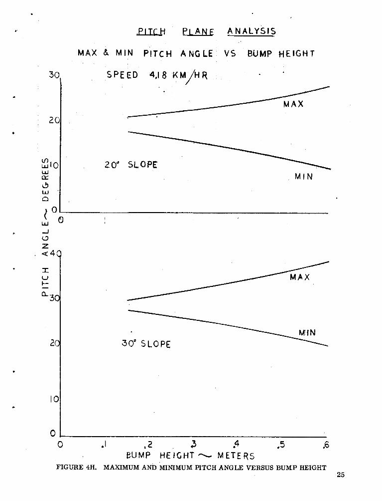
Care should be tak;-n in interpreting the curves of F igures 4G, 4H, 41, 45, 4K, and 4L. On Figure 1 the coordinate system i s shown with right-hand rotation and the Z axis a s positive up. the pitch angle positive in clockwise rotation. f igures resul t f rom operations on the level t e r r a in o r down a slope the curves maked I'minimum'' a r e counterclockwise (front of the vehicle displaced upward) variations of the vehicle 's pitch angle. When an obstacle was s t ruck with the vehicle going down a slope, the initial variation reduced the pitch angle. The tes t conditions were se t with the vehicle traveling down a grade because i t was felt that this represented a "worst case" condition and that the vehicle was m o r e likely to pitch over during such t e s t s . point for high obstaclss doubt a s to i t s stagility under these conditions for the 30° slope. pitch angles of 45 were reached. The c r i t i ca l angle is jus t above 50 .

This makes 1

Since the curves of the above

Even though the vehicle did not pitch ove r , i t did near the c r i t i ca l

Posit ive a t the two higher t e s t speeds, leaving some

0

The rancqom surface t r ave r se represents the LSV's CG while i t is driven over an i r r egu la r Lunar sur face . F o r the low amplitudes of the forcing function there is an indication that i r r egu la r surface perturbations wil l cause the LSV to r e x h a near ly constant frequency of oscillation at a near ly constant zmplitude. This , of course , would be changed by la rge spike-type i r regular ly-spaced obstacles , but this theory shou:.d hold as long a s the LSV does not leave the Lunar surface. F igures 4M and 4N show the time history t r a c e s of the CG displacements f o r the tes t s that were run, along with the forcing functions that were used. F igures 4 0

8

L

I

.

and 4 P show that the average CG displacement fo r random surface bumps is approximately two-thirds the average height of the bumps. be noted that for this tes t condition, the LSV did not leave the Lunar surface.

It should

2 . 3 CONCLUSIONS AND RECOMMENDATIONS

While this vehicle was tested using only one se t of parameters , the values of suspension and t i r e constants appear to be well chosen. instance, in previous studies (Task Order N - 2 2 ; Reference 1 ) i t was demonstrated by parametr ic studies of suspension sys tems that:

For

(1) Stiff suspension springs and t i r e ( spr ing) constants wi l l cause a grea te r CG displacement than soft spr ings while an LSV is t r a v e r - sing an obstacle with a given height. allow m o r e ringing af te r an obstacle is s t ruck. a lso is grea te r foi softer spr ings.

Softer spr ings, on the other hand, Initial vehicle settling

( 2 ) Greater damping will reduce settling t imes , but, in the c a s e of the LSV, wi l l cause grea te r icitial CG dlsplaceiiient {at higher vehicle speeds) when an obstacle is t raversed.

The choice of constants i s , therefore , a compromise.

Table I shows a comparison of the resu l t s found for a 6500 pound vehicle (Reference l ) , tes ted under severa l conditions, and the 4- wheel vehicle of this report . t ravers ing a 0.31 me te r obstacle at 8.36 Km/hr . used for a l l ca ses .

The resul ts a r e shown for each vehicle Step functions were

In the case of this vehicle, the suspension and t i r e constants This appears to be allow an initial vehicle settling of nearly 0.9 feet.

reasonable since the vehicle bottoms (in these t e s t s ) only for 0.62 me te r obstacles a t slow speeds. The suspension damping gave a performance s imi la r to that of a damping factor ( ’ ) of 0 .5 to 0.6. be within range since in control syst2ms the most common damping factor generally chosen is 0.7.

This appears to

Some difficulty with this vehicle was noted on higher slopes. The difficulty is not peculiar to this design o r suspension system. difficulty presents itself throrg h the effects of the low Lunar gravity. The margin of safety from turnover is low when the vehicle makes turns up s lopes o r makes Aclcerman t u m s with the full 24 --par t icular ly a t the higher recommended speeds. The mar gin of safety is a l so low when the vehicle s t r ikes large objects while gt>ing down slopes. Pi tch angle for the la t te r conditions reached 45O while overturn occurred at approximately 50 .

The

0 wheel on level t e r r a in

0

This type of task does not call f o r recommendations, and no recommendations a r e made.

9

t

FIGURE IA. 4 WHEEL LSV - MATHEMATICAL MODEL

RILL PLANK

c

c

FIGURE 1B. 4 WHEEL' ZSV - ROLL PLANE EQUATIONS

t a 1

Q, -Y, 4 M I I

FIGURE IC . 4 WHEEL ISV - ROLL PLANE EQUATIONS

R

12

FIGURE ID. 4 WHEEL LSV - MATHEMATICAL MODEL, PITCH PLANE, LEVEL T E R M I N

FIGURE i E . 4 WHEEL LSV - MATHEMATICAL MODEL, F'ITCH PLANE, VEHICLE ON SLOPE 13

FIGURE 1F. 4 WHEEL LSV - PITCH PLANE EQUATIONS

14

c

4

S P E E D KM/H R

u

FIGURE 2. CG DISPLACEMENT VERSUS SPEED 15

P I T C H PI ,AN& A N A L Y S I S

RATIO \OF M A X CG D I S P L A C E M E N T TO BUMP HEIGHT . .

VS BUMP H E i C h f

.

0 , I . 2 .3 .4 .5 ,G

BUMP HEIGHT METER c

FIGURE 3A. RATIO CG DISPLACEMENT.TO BUMP HEIGHT VERSUS 16 BUMP HEIGHT

b - PITCH P L A N E A , N A L Y S I S

M A X C G A C C E L E R A T I G N VS, BUMP H E I G H T

0 ,I 2 3 ,4 .J L; ,c

BUMP HEIGHT ?* METERS

FIGURE 3B. MAXIMUM'CG ACCELERATION VERSUS BUMP HEIGHT 17

-1 w

3 c

\ \ \ \

1 I

/ /

CrL N I

Y

\ \ \ \ \ \ \ \

r4

-e

n J

0

\ \ \

(Y X

33 -\ 4: \

CD 0

p.

nl

0

0 b H t-

3 !i r w - 3 w

r

I U I-

a. -

c

\ \ \ \

\ \ \ \ \ \ \

\ \

CY

Y 1 .

x

b.

. . -

0

C n c n J J w w w w.

w ' s I a.3 3 0

\ \

\ \ - I /

/ /

\ \ \ \

e f

\ \

\ \ \ \ \ \

i

(0

P

0

(9

N,

0 (D

0

.

20

\ . \ \ \ \

I

\ \ \ \ \

ck: \ I \

.e

C C

0 " S L O F E .

.5

FIGURE 4E. MAXIMUM CG ACCELERATION VERSUS BUMP HEIGHT

~ _ _ _ _ _

c

t

1 SEQUENTjIAL BUMPS - .

I , I I

E D 1 LINES ~I.N,DICATE ACCELESATION DUE E A R "EELS; S T R I K I N G BUMP

I

I !

c / z o o SLOPE /

I

. .

?

! .

3 0 " SLOPE

0 I 2 a 4 5 6 BUMP HEfGHT- M E T E R S

23 FIGURE 4F. MAXIMUM CG ACCELERATION VERSUS BUMP HEIGHT

2(

I C

0

f2'

. . - : I

MAX & M I N P I T C H ANGLE VS BUMPHEIGHT

too S L O P E

t .5 6 C 0 ,I .2 .3 .4

BUMP H E I G H T - METERS 24 FIGURE 4G. MAXIMUM AND MINIMUM PITCH ANGLE VERSUS BUMP HEIGHT

4'

I.

20

3 0 W LT

w . c3 n IO

M A X &. M I N PITCH A N G L E VS BUMP HEIGHT

c

20" SLOPE M I N

-

30° SLOPE

0 .I , z 3 *4 ' 5 ,6 EUMP H E I G H T - METERS

FIGURE 4H. MAXIMUM AND MINIMUM PITCH ANGLE VERSUS BUMP HEIGHT 25

IC

C

- 10

In w W ck (3 w r3

I W -#J i3 z Q

I 40 -

Q

3c

20

-I 0

M A X & . M I N P I T C H ANGLE VS BUMP HEIGHT

S P E E D 8.36 K M / H ? M A X

.

FIGURE 41, MAXIMUM AND MINIMUM PITCH ANGLE VERSUS BUMP HEIGHT 26

P I T C H P L A N E A N A L Y S I S .

M A X d M I N P I T C H ANGLE VS BUMP HEIGHT

20° ' SLOPE

30° : S L O P E

M I N

0 . I .2 .d .4 ,5 &6 BUMP HEIGHT- M E T E R S

FIGURE 45. MAXIMUM AND MINIMUM PITCH ANGLE VERSUS BUMP HEIGHT 27

w w &

Ll 0

W J

0

PlTC H P L A N E A N A L Y S I S

M A X ' h M I N PiTCti A N G L E VS BUMP HEIGHT

S P E E D 16.72 KM/HR

0' SLCPE

io" SLOPE

M N

-I c 0 .s

MIN

,6

FIGURE 4K. MAXIMUM AND MINIMUM HTCH ANGLE VERSUS BUMP HEIGHT 28

c

t

4c

3

t

I U I-

a. - 2c

c

C

P I T C H P L A N E A N A L Y S I S

MAX- & M I N PITCH A N G L E VS BUMP HEIGHT

S P E E D 1672 KM/HR

M I N

30' .SLOPE Mf N

.3 .4 -5 b 0 1 .2 0

B U M P H E I G H T - M E T E R S FIGURE 4L. MAXIMUM AND MINIMUM PITCH ANGLE VERSUS BUMP HEIGHT

29

t

I

I I I I

I

f -

_____-_________ - _ - - _ ___-----________

I I t _---_____ ~

I

I I

--- - _---------- L I _ . . . . . . , . , _ _

I

I I I I I I I I I I I L I

I I I I I I I l l 1 I I I I 1 I I I I 1

I

I

I I

FIGURE 4N. RANDOM SURFACE TRAVERSE 31

, .2

.' I

0

32

P E A K B U M P H E I G H T S VS T I M E

41

01 0 IO

FIGURE

20 30 4 0

T I M E 'L SEC,

40. RANDOM SURFACE TRAVERSE

8

L

h

C

L

i. T - i ! '

.-.

I

. .

. . v: ' 3 u, 4 a,

. L A - & ,

4 ci ! I u

' I ' I

i

! I

t I !

I

i I

i .

i

. I

. ,

i

!

P E A ' K EWP HEIGHT VS T I M E

t

c3 = ,4 - w I

0,

3 = .2 m J

Y Q: w

e a 0 , 0 I O 2 0 30 40 50

FIGURE 4P. RANDOM SURFACE TRAVERSE 33

I

- 4 - 0 -12 -16 - 2 0 - 24

WHEEL A N G L E - D E G R E E S

FIGURE 5A. ROLL ANGLE VERSUS WHEEL ANGLE

.

. * . - . .. ..

ROLL ANGLE V.9 WHEEL A N G L E I

0 ,

-IO0 SLOPE . .

/ ’ ’OVERTURN

- - - - / / : I S K I D POINT

8.36

0 4 8 12 16 20 24

WHEE. L ANGLE- D E G R E E S

FIGURE 5B. ROLL ANGLE VERSUS WHEEL ANGLE 35

STEERING A N A L Y S 15

36

ROLL ANGLE V S WHEEL A N G L E 20° SLOPE

.

0 4 8 i Z 16 20 24

WHEEL ANGLE- D E C R E E S

FIGURE 5C. ROLL ANGLE VERSUS WHEEL ANGLE

STEER( NG A N A L Y S I S

WHE€L ANGLE ROLL A".GCE V S I

3Go SLOPE

-4;

-4 / /

/

8.3 6

KM/H R

M I N P z . 3 t

- 3c

. 0 0 4 8 . 12 . I6 2 0 L 34

FIGURE 5D. ROLL ANGLE VERSUS WHEEL ANGLE 37

STEER1 NG A'NALYS 15 . M A X ROLL A N G L E ' A C ~ E l E R A f i O N VS SPEED

E E L C LE

b 4 8 I2 16 20 1

S P E E D - KM/HR

FIGURE 5E. MAXIMUM ROLL ANGLE ACCELERATIONS VERSUS SPEED 30

c

S T E E R I N G ANALYSIS

- SPEED VS W H E E L A N G L E

O* S L O P E

8 12 16 2 0 24 0 4

YHEEL ANGLE - DEGREES

FIGURE 5F. SPEED VERSUS WHEEL ANGLE 39

0

ST EER I NG PNALYS IS

S P E E D VS WHEEL A N G L E

IO" S L C P E

4 8 12 I6 2 0

WHEEL A N G L E - D E G R E E S

24

FIGURE 5G. SPEED VERSUS WHEEL ANGLE 40

.

' I

I

.. 1

I I i , ,

/&=. 2 STATTC S K I D ,A= ,I3

0 4 8 12 I6 2 0 24 U

WHEEL A N G L E - DEGREES

FIGURE 5H. SPEED VERSUS WHEEL ANGLE 41

cy

42

I STEERING ANA LYS I S i * t i

1 ! S .REED[VS W H E E L A N G L E

\

4 _ . ..

!

I

. . ,

0 - 8 -12 -16 - 2:o - 2:4

W H E E L A N G L E - D E C e E E S

FIGURE 51. SPEED VERSUS WHEEL ANGLE

!

*

I

- I i .

w

c3 z - i o

* -2; -I -I 0 cy:

X Q 2

-18

- I 4

- IO I

I

J 5 2 ,M, SEQUiENT1A.L: BUMPS . I

O V E R T U R ~ ~ O C ~ ~ U R S O N ' O A S H E D L I N E x -OVERTURN HAS O C C U ~ E D ~ - 24e

WHEEL < / ANGLE

0" SLOPE / /

0

- IO0 S L O P E

-24' /

/ - I 2 '

20 0 4 8 12 16 S P E E D KM/HR

FIGURE 6A. MAXIMUM ROLL ANGLE VERSUS SPEED 43

E

S T E Ef?l NG ANALYSIS

MAX ROLL ANGLE Vs SPEED

.I54 M, SEOUENTIAL @lJMPS

G V € e T U R N OCCURS 'ON D A S H L D L I N E X - G K R T U R N HAS CCCURED

- 3 0 ° SLOPE

/ / 6'

0"

O T 0 4 8 12 16 20

S P E E D - KM/HR

FIGURE 6B. MAXIMUM ROLL ANGLE VERSUS SPEED

.

44

*

M A X ROLL A N G L ~ vs SPEED

,308 M, S E 9 U E N T t A L BUMPS x -24' WHEEL /

. ANGLE 0VERTUR.N O C C U R S O N /

DASHEb LINE / '

/ X-CVERTURN HAS

/ C C C U R E D - t ;

0 2 /

/ i 0" SLGPE /Y,- ul

W ck= 0

6 *

oo

LlJ : n ' 4

1. W J 13

' 2 0 a / - 2 4 ' J -.t 0 Qf

X Q 2

.I - 2

I

/ - I 2.'

-6" -10' SLOP E

! * o 4 8 12 I6 20 S P E E D - KM/HR

FIGURE 6C. MAXIMUM ROLL ANGLE VERSUS SPEED 45

S T EE R I N G ANALY S 1s I

MAX RGLL A N G L E V S SPEED

$

e 3 O 8 M SEQUENTIAL BUMPS -

O V E R T U R N OCCUf?S ON DASHED L I N E S X - O V E R T U R N H A S O C ~ U R E D

46

-30" S L O P E - 24' X

/ WHEEL ANGLE

0 4 8 I2 16 20

SPEE D - R

FIGURE 6D. MAXIMUM ROLL ANGLE VERSUS SPEED

I .

/ DASHED LINE / X-OVERTUI?N H A S OCCURED

/ I *

l -

l -

,S T E E R l NG A N A LY S 1 S

N A X ROLL ANGLE V S SPEED

.6l M, S E Q U E N T I A L BUMPS

-12 I -12'

0 4 8 12 16 2 G S P E E D - K M / H R

FIGURE 6E. MAXIMUM ROLL ANGLE VERSUS SPEED 47

m W W

0 W a

a

LJ -I 0 z <--48 J J 0 rr

X

2

- 44

a

- 40

0

S T E E R I N G A N A L Y S I S ~

I O V E R T U R N OCCURS ON EASHtfE3 L I N E X - O V E R T U R N H A S O C C U R E D

-30' SLOPE WHEEL A N G L E

-6'

0 4 8 12 I G 3.0

S P E E D - KM/HQ

FIGURE 6F. MAXIMUM ROLL ANGLE VERSUS SPEED 48

TABLE I. COMPARISON OF THE 4-WHEEL VEHICLE WITH VEHICLES TESTED PREVIOUSLY

Suspension Constant, L b / F t .

c

Ti re Constant Lb /F t .

Suspension Damping , Lb/Ft /Sec .

T i r e Damping, Lb/Ft /Sec .

Max. CG Displacement, Meters

Settling Time , Seconds

Ref. 1 V ehic 1 e

1000

500

125

0

0.54

9

Ref. 1 Vehicle

2000

500

125

0

0 .6

25

Ref. 1 4-Wheel Vehicle Vehicle

1000 725

500 600

500 150

0 1 5

0.57 0.58

12 7

49

PART I1 SIX WHEEL ARTICULATED VEHICLE

-

51

3.1 R O L L PLANE ANALYSIS

The mathematical model and equations of motion for the rol l plane analysis a r e shown in F igures 7A, 7B, 7C, and 7D. were written pr imar i ly for studying the s teer ing and studying the effects of LSV's t r ave r se in an object with the wheels of only one s ide of the vehicle.

These equations

The use of the equationk elements which contain M and Mb will be explained i n Section 3 . 2 and in (F igu re C3) Appendix e. wise, the equations a r e written in the usual manner .

Other-

The analog computer diagram and data for simulating the roll plane of the six wheel art iculated vehicle a r e shown in (F igures D1 and D2) Appendix D.

3 . 2 PITCH PLANE ANALYSIS

The mathematical model and equations of motion for the pitch plane analysis a r e shown in F igures 7E and 7 F . ly developed to examine the vehicle resonance, the vehicle displacement and pitch angle resulting f rom a forcing function applied to all wheels simultaneously, and the vehicle response to forcing functions applied to three se t s of wheels (The wheels of an axle form a se t ) , sequentially. The la t te r s imulates the LSV's striking a ledge.

This model was p r imar i -

The only unusual features of the equations of motion a r e the last two elements of equation (5 ) and the last element of equation (6) (F igure 7 F ) . equations ( 7 ) and (8) oaf Figure 7F . shown in Figure C3 of Appendix C, to simulate the resu l t s of bending modes in the vehicle spr ing coupling b a r . is a fourth-or higher order-equation which makes it imprac t ica l for a medium-sized analog computer. The last element of equation (5) r e - presents forces set-yp by the shear at the point of spr ing ba r and the main module contact, and the klement preceding the last element represents the moment on the spring ba r at the same point of contact. The last element of equation (6 ) represents the main module force on the t r a i l e r module .

The M and Mb of these equations a r e developed as These equations were developed, as

The t r u e representation of the l a t t e r

The computer diagram and data to be used in the pitch plane analysis a r e shown in (F igures C1 and C2) Appendix C.

-~

52

.

FIGURE 7A. LSV-6 WHEEL -ARTICULATED, MATHEMATICAL MODEL

53

FIGURE 7B. LSV-6 WHEEL -ARTICULATED, ROLL EQUATIONS

54

1 J

FIGURE 7C. LSV-6 WHEEL - ARTICULATED, ROLL EQUATIONS

55

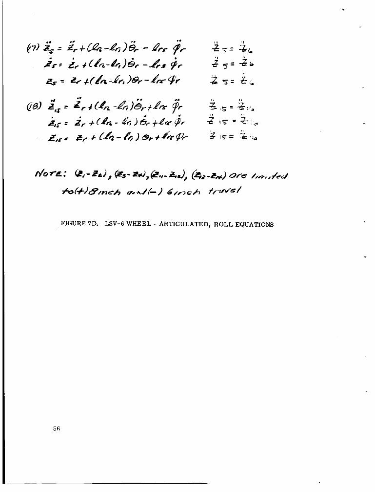
FIGURE 7D. LSV-6 WHEEL - ARTICULATED, ROLL EQUATIONS

56

FIGURE 7E. I.STJ-6 WHEEL - ARTICULATED, MATHEMATICAL MODEL, PIlCH PLANE

I FIGURE 7F. LSV-6 WHEEL - ARTICULATED, PITCH EQUATIONS

58

I

r

PART 111

PRELIMINARY STUDY O F LSV STEERING CONTROL

59

PRELIMINARY STUDY O F LSV STEERING CONTROL

Figure 8 i s a prel iminary block diagram to be used a s a bas is for studying the LSV steer ing control. the control a r e shown. The system, as shown, is general in a l l a r e a s concerning sensors , instruments and limits. A digital, analog--or combination digital-analog -control system can be studied by proper models in the appropriate blocks.

Only the major loops of

Two modes of operation a r e shown--remote and manual. The remote loop, marked "Mode 2 " , is shown for Ear th- remote study purposes. However, by changing t ime delays the same loop can be us - ed for Lunar-remote surface operations. "Mode 1'' is the manual control loop operated by the astronaut, and with the exception of the coding, de- coding (computer) and radio t ransmission functions, is s imi la r to Mode 2. a t any t ime.

Only one of the modes of steering ( remote o r manual) can be used

Speed i s a parameter which directly affects the ability to s t ee r . It is not par t of the direct steering control, but i s added for both modes where i t is applicable.

The capability for changing s teer ing modes is shown. Al- though scuff steering is not shown, i t could easily be added to the s t e e r - ing mode block which controls the "Master Wheel Position".

In a l l steering modes, except scuff steering, i t will be neces- s a r y to control both front wheels a s a unit and both r e a r wheels as a unit. This i s shown on the schematic a s a synchronizer in the s teer ing motor loops feedback.

t

Speed, rol l , and pitch l imits which have been found f rom

Other features result ing f rom the completed dynamic studies dynamic studies to be very 'desirable, have been included in the study diagram. can be shown in the expansion of the block marked "Vehicle Position".

60

5.0 SYMBOLS

C. G.

D

E1

g

h

Ix

0

IY

0 K

lm( )

1

0 M

t

V

X 0

y( )

0 Z

e

!?

9

Center of Gravity

Damping constant, l b / f t / s ec

Module of Elast ic i ty , lb-ft

Gravity, f t / s e c

Height of C. G, Ft.

2 Moment of Iner t ia about X ax is (Roll P lane) , Slug-ft

Moment of Iner t ia about Y axis (P i tch plane), Slug-ft

2

2

2

Spring constant, lb/fg

Dimension (Main Module), f t

Dimension (Rear Module) , f t

Mass, Slugs

TIME, seconds

Vehicle velocity, Km (mi l e s ) p r h

Length Dimension (4 wheel vehicle) , f t

Width dimension (4 wheel vehicle), f t

Ver tic a1 Dis plac em ent , f t

Pitch angle, deg rees

Roll angle, degrees

Yaw angle, degrees

Subsc riDts:

1

2

3

4

Right F ron t Wheel Main Module

Right F ron t Chass i s Main Module

Right R e a r Wheel Main Module

Right Rea r Chass i s Main Module

62

5

6

7

11

12

13

14

15

16

m

of

If

o m

im

o r

i r

l-

Right T ra i l e r Wheel

Right T r a i l e r Chass i s

Coupling Between Main Module and T r a i l e r

Left F ron t Wheel Main Module

Left F ron t Chass i s Main Module

Left Rea r Wheel Main Module

Left Rea r Chass i s Main Module

Left Rea r T r a i l e r Wheel

Left R e a r T ra i l e r Chassis

Main Module

Bottom of Right F r o n t Wheel

BottDm of Left F ron t Wheel

BottDm of Right Rea r Wheel (6 wheel vehicle)

Bottom of Lef t Rear Wheel (6 Wheel vehicle)

Bot tom of Right T ra i l e r Wheel ( 6 wheel vehicle)

Bottom of Right Rea r Vheel (4 wheel vehicle)

Bottom of Left T r a i l e r Wheel (6 wheel vehicle)

Bottom of Left Rear Wheel (4 wheel vehicle)

Rea r Module ( T r a i l e r )

63

REFERENCES

1. "Apollo Logistics Support Systems MOLAB Studies- Mission Command and Control" by Arch W. Meagher and Harvey Ryland, ALLS BULLENTIN 006, September, 1964.

BIBLIOGRAPHY

1. "Elements of Strength of Materials", by Timoshienko and MacCullough, D. VanNostrand Co. , Inc.

64

6 .0 APPENDICES

1 -

65

INDEX

APPENDIX A

FOUR WHEEL VEHICLE --PITCH PLANE DATA AND COMPUTER MODELS

APPENDIX B

FOUR WHEEL VEHICLE--ROLL PLANE DATA AND COMPUTER MODELS

APPENDIX C

SIX WHEEL ARTICULATED VEHICLE-PITCH P L A N E ANALYSIS

Page

67

75

89

APPENDIX D

SIX WHEEL ARTICULAT ED VEHICLE-ROLL P L A N E ANALYSIS 99

APPENDIX A

FOUR WHEEL VEHICLE--PITCH PLANE DATA AND COMPUTER MODELS

67

FIGURE AIA. FOUR WHEEL VEHICLE (PITCH PLANE)

68

c

- \oo

FIGURE AIB. FOUR WHEEL VEHICLE (PfTCH PLANE)

69

I --c---- 3 ul

.

70

.

i A L

r"

3

X

w' d

72

FIGURE AIF. COMPUTER POT-SETTING QUANTX'ITES - 4 WHEEL VEHICLE (PITCH PLANE ANALYSIS)

73

FIGURE A2. DATA AND CALCULATIONS - 4 WHEEL VEHICLE (PITCH PLANE ANALYSIS)

I:

APPENDIX B

FOUR WHEEL VEHICLE

ROLL P L A N E DATA AND COMPUTER MODELS

75

.

.

FIGURE BIA. ROLL PLANE - 4 WHEEL VEHICLE

76

t I

1

-2 5 (i ,,- i ,a )

FIGURE BIB. ROLL PLANE - 4 WHEEL VEHICLE

D---

77

to

I

I

c

FIGURE BIC. ROLL PLANE - 4 WHEEL VEHICLE

78

FIGURE BID. ROLL PLANE - 4 WHEEL VEHICLE

79

Y 1

FIGURE BIE. ROLL PLANE - 4 WHEEL VEHICLE

80

FIGURE BIH. POT SETTINGS - 4 WHEEL VEHICLE (ROLL PLANE ANALYSIS)

83

FIGURE B2. DATA AND CALCULATIONS - 4 WHEEL VEHICLE (ROLL PLANE ANALYSIS)

84

?OK

FIGURE B3. CALCULATIONS FOR PERFORMANCE ON A SLOPE - ROLL PLANE

85

SIMULATION O F THE 4 WHEEL VEHICLE ON A SLOPE ROLL PLANE ANALYSIS

The simulation of the vehicle on a slope (in the rol l plane) was accomplished by using the computer diagram f o r the rol l plane analysis and adding a constatly-applied torque in the rol l angle equation. This torque was developed as shown in F igure B3 by shifting the forces on the right and le f t wheels. right and left vehicle a r e off the lunar surface. However, a s expected, this did not occur for any of the perturbations used in the rol l plane studies. The pertrubations (forcing functions) were added to the s imu- lation as in other studies, and should not be confused with the torque described above.

This simulation is not applicable when both

86

.

.

DEVELOPMENT O F THE FORCING FUNCTION FOR EXAMINING ACKERMAN STEERING ---4 WHEEL VEHICLE

In developing the computer forcing function for examining Ackerman s teer ing, two assumptions were made. First, the turning radius was defined as the radius of the c i r c l e described by the vehicle CG in a turn, and second, there is no skidding of the vehicle f ront wheels in the turn. speed while in the turn. All these assumptions lead to the examination of a "worst case" condition with safety fac tors included in the computer simulation.

The vehicle was assumed to maintain constant

As indicated in F igure B4 and a s a resu l t of the above assumptions, the velocity of the vehicle CG and the velocity of the steering wheels a r e normal to the turning radius. the vehicle a r e calculated for wheel angles of 6, 1 2 , 18, and 24 degrees by using the vehicle,width and length, as shown.

Therefore turning radius of

The next s tep calculates the t ime required for the vehicle to make a complete 90-degree turn using the vehicle speed (4.18, 8.36, and 16.72 h / h r and each of the wheel angles.

Since the ent i re momentum of the vehicle (in the original direction of t rave l ) changes during the execution of 90-degree turn, the force '

(acceleration l i m e s m a s s ) toward the center of the turning c i r c l e is calculated. ing moment) which i s applied to the center of gravity.

This forces t imes the CG height fo rms a couple (overturn-

The above couple (or torque) represents the maximum value of the overturn force on the vehicle when the vehicle has reached the position of full turning rate . the t ime for turning r a t e to become maximum and the t ime for the wheel angle (physical accomplishment time-delay) to reach the maximum. These a r e found by adding the ra te to the given time-delay of 6 O per second. Normally Ackerman steering can be accomplished on the computer by a half-sine wave forcing function. However, as shown, the frequencies of the forcing functions for this simulation a r e so smal l that a r amp function (0 to maximum torque) was applied and held af ter maximum torque was reached.

Two time-delays a r e involved:

87

.

FIGURE B4. ROLL MOMENT - STEERING ( 4 WHEEL VEHICLE)

88

I ' .

APPENDIX C

SIX WHEEL ARTICULATED VEHICLE - PITCH PLANE ANALYSIS

L

89

- too

FIGURE CIA. 6 WHEEL ARTICULATED PITCH PLANE ANALYSIS

90

.

FIGURE CIB. 6 WHEEL ARTICULATED PITCH PLANE ANALYSIS

91

FIGURE CiC. 6 WHEEL ARTICUJATED PITCH PLANE ANALYSIS

92

FIGURE CID. 6 WHEEL ARTICULATED PITCH PLANE ANALYSIS

93

c 1

/O '

FIGURE C2. BASIC DATA AND CALCULATIONS - 6 WHEEL ARTICULATED VEHICLE (PITCH PLANE ANALYSIS)

L

DEVELOPMENT O F THE MOMENT ON THE CONNECTING SPRING- BAR BETWEEN THE ELEMENTS O F THE 6-WHEEL ARTICULATED VEHICLE

Since the flexible coupling between the main module and the t r a i l e r of the 6 wheel art iculated vehicle w a s found to function with higher bending modes than the f i r s t , it was necessary to develop a simple means of placing this function on the computer. o rde r equ.xtions, normally used, proves to be impractical . F igures D3A and D3F show a simplified means of finding the coupling ba r ( spr ing) bending moment a t the connection point of each module. is shown, the formula for the end deflection of a cantilever beam and the mcment on the end of the cantilever beam is used. The E1 and the length of the coupling ba r a r e given in the data.

Programming the higher

As

The moments on the coupling bar a r e of in te res t in the computer simulation only a t the bar-module contact point, -- The moments a r e derived, as shown on Figures C3A and D3B by equating the displacement between the contact points represented by two equations--the deflection equation and the equation formulated smal l angle theory. The moments thus derived a r e used, along with the b a r shear forces at the contact points, in equations on pages and of the text. Fur ther explanation of the combination of the moments and the shear forces is given in the text.

95

x I -

.

FIGURE C3A. DEVELOPMENT OF MOMENT ON CONNECTING SPRINGBAR ( 6 WHEEL VEHICLE)

h

FIGURE C3B. DEVELOPMENT OF MOMENT ON CONNECTING SPRING-BAR ( 6 WHEEL VEHICLE)

97

APPENDIX D

SIX WHEEL ARTICULATED VEHICLE

ROLL PLANE ANALYSIS

99

.

Z 4 Z I 0-n . I 00

z t ) -2 I 1

- / o o

r

c

I --p- i,,

FIGURE DIA. 6 WHEEL ARTICULATED VEHICLE - ROLL PLANE ANALYSIS

i'ob

t

V

c

FIGURE DIB. 6 WHEEL ARTICULATED VEHICLE - ROLL PLANE ANALYSIS

101

102

FIGURE DIC. 6 WHEEL ARTICULATED VEHICLE - ROLL PLANE ANALYSIS

c

FIGURE DID. 6 WHEEL ARTICULATED VEHICLE - ROLL PLANE ANALYSIS 103

z,-z, I

z,-z, I

- - I - 0 m

ID- -+-

OW

c

FIGURE DIE. 6 WHEEL ARTICULATED VEHICLE - ROLL PLANE ANALYSIS

I04

-2,

, I

I 8

-2 w

7 L M

-e,

- @ M

I

Zr,

N\ ..

7

Z,

. FIGURE DIF. 6 WHEEL ARTICULATED VEHICLE - ROLL PLANE ANALYSIS

105

z,- 20,

25- Z O l

I I

z;,-z,, .z rc- z ,c I .

I ,

-D- U

-.8c

c

FIGURE DIG. 6 WHEEL ARTICULATED VEHICLE - ROLL PLANE ANALYSIS

'i 06

sw 00

-100

r

-L lMlrEf i

107

FIGURE DII. POT SETTINGS - 6 WHEEL ARTICULATED LSV (ROLL PLANE ANALYSIS)

108

.

FIGURE DIJ. POT SETTINGS - 6 WHEEL ARTICULATED LSV (ROLL PLANE ANALYSIS)

109

FIGURE D2. BASIC DATA AND CALCULATIONS - 6 WHEEL ARTICULATED VEHICLE (ROLL PLANE ANALYSIS)

1 i o

__

DISTRIBUTION

c

INTERNAL

DIR DEP-T

R-DIR R-AERO-DIR

-S -SP (23)

-A (13)

-A -AB ( 15) -AL (5)

R-ASTR-DIR

R-P& VE-DIR

R-RP -DIR -J (5)

R-FP-DIR R-FP (2) R-QUA L-DIR

-J (3) R-COMP-DIR R-ME-DIR

-X R-TEST-DIR I-DIR MS -IP MS-IPL (8)

EXTERNAL

NASA Headquarters MTF Col. T. Evans MTF Maj. E. Andrews (2) MTF Mr. D. Beattie R-I Dr. James B. Edson MTF William Taylor

Scientific and Technical Information Facility P.O. Box 5700 Bethesda, Maryland

Attn: NASA Representative (S-AK RKT) (2)

Manned Spacecraft Center Houston, Texas

Mr. Gillespi, MTG Miss M. A. Sullivan, RNR John M. Eggleston C. Corington, ET-23 (1) William E. Stanley, ET (2)

Donald Ellston Manned Lunar Exploration Investigation Astrogeological Branch USGS Flagstaff, Arizona

Langley Research Center Hampton, Virginia

Mr. R. S. Osborn

Kennedy Space Center K-DF Mr. von Tiesenhausen

contractor - nasa steering effects and the effects of having the vehicle traverse obstacles while in...

Documents