Continuum effects for the mean-field and pairing properties ofweakly bound nuclei

K. Bennaceur,1 J. Dobaczewski,2−4 M. P loszajczak1

1Grand Accelerateur National d’Ions Lourds (GANIL), CEA/DSM – CNRS/IN2P3, BP 5027,F-14021 Caen Cedex, France

2Institute of Theoretical Physics, Warsaw University, Hoza 69, PL-00681, Warsaw, Poland3Department of Physics, University of Tennessee, Knoxville, Tennessee 37996

4Joint Institute for Heavy Ion Research, Oak Ridge, Tennessee 37831

Abstract

Continuum effects in the weakly bound nuclei close to the drip-line are in-vestigated using the analytically soluble Poschl-Teller-Ginocchio potential.Pairing correlations are studied within the Hartree-Fock-Bogoliubov method.We show that both resonant and non-resonant continuum phase space is ac-tive in creating the pairing field. The influence of positive-energy phase spaceis quantified in terms of localizations of states within the nuclear volume.

PACS numbers: 21.10.Gv,21.10.Pc,21.60.-n,21.60.Cs

Typeset using REVTEX

1

I. INTRODUCTION

In the theoretical description of drip-line nuclei, the residual coupling between boundstates and the continuum is an essential element of the physical situation. Standard de-scription of many-fermion systems [1] most often invokes the concept of the Fermi sphere ofoccupied states, and correlations of particles occurring mostly in a narrow zone of the phasespace around the Fermi surface. It is obvious that whenever the Fermi energy is close tozero, which by definition is the case in weakly-bound systems, the zone of correlated statesmust incorporate the phase space of particle continuum.

Among different types of correlations which are important in nuclei, in drip-line nucleipairing plays a singular role, because the intensity of pairing correlations is a determiningfactor in establishing position of the last bound nucleus. Indeed, in any isotopic chain, thelightest unbound nucleus corresponds to an odd-N system in which the pairing energy ∆,missing in the binding of the odd neutron, equals to the loss of the mean-field binding whenthis neutron is shaken off, see e.g. discussion in Refs. [2–4]. Therefore, study of pairingcorrelations in weakly bound systems is since many years one of the leading subjects ofanalyses predicting properties of very neutron rich nuclei.

After early analyses, see Refs. [5–11] and references cited and reviewed in Refs. [12,13],the field has now become very active, due to projected developments in radioactive ion beamfacilities throughout the world. In particular, methods based on using the Skyrme effectiveinteraction and on the Hartree-Fock-Bogoliubov (HFB) approximation have been applied toboth spherical [12–16] and deformed [17–19] drip-line nuclei. Spherical drip-line nuclei havealso been studied by using the Gogny interaction and the HFB method [12,16]. In addition,methods based on the relativistic mean field approach [20], with pairing correlations includedwithin the Hartree-Bogoliubov approximation, have been extensively used to study variousphenomena in spherical drip-line nuclei [21–28]. Structure of pairs have also been studied bysolving the two-body problem exactly, including the continuum effects [29], and the influenceof particle resonances on pairing properties have been analyzed in terms of the BCS method[30,31].

In the framework of the mean-field approximation, pairing correlations are consistentlyincluded within the variational Hartree-Fock-Bogoliubov (HFB) approach [32]. Such anapproach is appropriate for studying bound nuclei, i.e., systems with negative Fermi energy,in which the effects of continuum amount to ensuring that the obtained many-body statesare stable with respect to virtual excitations of particles and pairs of particles to positive-energy phase space. In this study we do not consider scattering problems, for which the wavefunctions are not localized and describe physical situations of particles being scattered off,or emitted by nuclei. On the other hand, bound states, however weakly bound, are alwayslocalized and discrete, and such are the basic features of the approach discussed in the presentstudy. A properly executed variational theory, and such is the HFB approach, always yieldslocalized bound states. Moreover, when solved in the coordinate representation, the HFBmethod takes fully into account all the mean-field effects of coupling to the continuum[6,9,12].

The HFB equations are relatively easy to solve in the matrix representation, i.e., afterexpanding the quasiparticle wave functions on a suitable basis. When the harmonic oscil-lator (HO) basis is used, the method is inappropriate for a description of weakly-bound

2

states, because of an incorrect asymptotic properties of the HO wave functions [12]. How-ever, recently developed methods, which use the so-called transformed harmonic oscillatorbasis [27,33], combine the simplicity of the basis expansion with the corrected asymptoticbehavior. In this way, large-scale deformed HFB calculations in drip-line nuclei becomerecently possible [34]. Another method proposed [35] for a solution of the HFB equationsrelies on using the natural orbitals; although very promising in principle, it has not beenfully implemented in practice yet.

Apart from these attempts, most of the HFB calculations in drip-line systems per-formed to date use the coordinate representation. Most of these studies have been re-stricted to spherical symmetry, for which the coordinate-space problem amounts to solvingone-dimensional equations. Three-dimensional solutions for deformed nuclei have also beenobtained by using hybrid methods of solving the HFB equations in the basis of coordinate-space Hartree-Fock (HF) wave functions [17–19]. All such algorithms use wave functionsapproximated on spatial grids of points, and the continuum discretized by suitable large-box boundary conditions. Numerical stability and convergence properties of these methodshave been thoroughly tested, and are considered to be sufficient for the current mean-fieldapplications, however, more efficient techniques, using the so-called basis-spline Galerkinlattices [36] are also being constructed.

In view of the fact that pairing properties of nuclei near the stability valley are mostoften treated within the BCS approximation, there have been numerous attempts of usingthis simpler method in drip-line nuclei too, see e.g. Refs. [37–39,30,31]. Various tests show[6,12,40–42], however, that such an approach is often unstable and/or divergent. A mean-ingful use of the BCS approximation to the HFB method requires especially careful andconscious treatment, which may, in fact, cost more effort than a straightforward applicationof the more involved, but certain HFB method itself.

Resonance contribution into the HF+BCS equations was recently studied in Refs. [30,31].This approximate method can take into account the effect for well separated resonances,when the resonance energies do not depend strongly on the box size or the cutoff procedure.More refined treatments of particle continuum have also recently become available [43,44],although they have not yet been combined with pairing correlations. On the other hand,intuition gained in solving the BCS problem in nuclei tells us that low-energy continuumstates must more generally contribute to pairing correlations of drip-line nuclei. In thepresent paper we aim at quantifying this influence in the framework of the HFB method.

The full-scale HFB calculations and/or the analytically soluble models with realisticpotential shapes are invaluable tools for understanding phenomena associated with the con-tinuum in weakly bound systems. In this work, we shall employ the Poschl-Teller-Ginocchio(PTG) average potential, which is an extension of the textbook Poschl-Teller potential[45–47], proposed by Ginocchio [48]. It belongs to a broader class of analytically solvablepotentials proposed some time ago by Natanzon [49]. The PTG potential has the mainfeatures of the nuclear mean field, namely, flat bottom, diffused surface, and asymptoticfreedom (i.e., it exponentially vanishes at large distances). For this potential, analyticalsolutions are available for wave functions and energies of the single-particle bound statesand resonances. These advantages make it very useful for applications to nuclear structureproblems [50,51].

In Sec. II, we recall the most important features of PTG potential, in particular those

3

concerning the parametrization of the diffuse surface. Sec. III presents some essentials ofresonance phenomena and discusses their relation with poles of the S-matrix. In Sec. IV, de-tails of the single-particle wave functions and single-particle resonances in the PTG potentialare recalled and, in particular, properties of wave function corresponding to weakly bound,virtual and resonance states are discussed. Sec. V contains main results of this work. Hereresults of the HFB calculations with the PTG input are discussed, and the pairing couplingto single-particle states in the continuum is analyzed. Finally, Secs. VI and VII summarizeperspectives of further investigations and the main conclusions we draw from this study,respectively.

II. POSCHL-TELLER-GINOCCHIO POTENTIAL

The PTG potential depends on four parameters: Λ which determines its shape anddiffuseness, ν which defines its depth, s (in fm−1) which is a scaling factor that can beadjusted to obtain a given mean radius of the potential, and a, which allows to account foran effective mass of the particle. In the present study, the effective mass is not discussed,and therefore we take a=0, for which the radial PTG potential is defined as:

VPTG(R) =h2s2

2m(v(R) + c(R)) , (2.1)

where m is the mass of free particle, v(R) is the central part,

v(R) = − Λ2νLj(νLj + 1)(1− y2) +

(1− Λ2

4

)(2.2)

× (1− y2)(2− (7− Λ2)y2 + 5(1− Λ2)y4

)and c(R) is a (nonstandard) centrifugal barrier,

c(R) = L(L + 1)(

1− y2

y2

)(1 + (Λ2 − 1)y2). (2.3)

Dimensionless variable η is proportional to the radial coordinate R,

η = sR, (2.4)

and y is implicitly defined by the expression:

η =1

Λ2

[arctanh(y) +

√Λ2 − 1 arctan(y

√Λ2 − 1)

], (2.5)

where 0 ≤ η ≤ +∞ and, consequently, 0 ≤ y ≤ 1.Parameter Λ can take any positive value. (Potentials with Λ<1, for which in Eq. (2.5)

function arctan changes into arctanh, will not be considered in the present study.) Inprinciple, parameters Λ, ν, and s can take different values for every value of L and j.However, below we use (Lj)-independent values of shape parameter Λ and scaling factor s.On the other hand, as indicated in Eq. (2.2), values of depth parameter ν are independently

4

chosen for each L and j, so as to obtain ’reasonable’ single-particle spectra, and in particular,to simulate the spin-orbit splitting of single-particle levels which is absent in the PTGpotential.

Problem of the nonstandard centrifugal barrier (2.3) deserves a few words of discussion.At the origin (η → 0), y decreases as η, y → η, and therefore,

s2c(R) −→ L(L + 1)

R2(2.6)

becomes the standard centrifugal barrier. On the other hand, at large distances (η → ∞),1−y decreases exponentially, i.e.,

c(R)−→4Λ2e−2Λ2(η−η0), (2.7)

where

η0 =

√Λ2 − 1

Λ2arctan

√Λ2 − 1, (2.8)

and the nonstandard PTG centrifugal barrier exponentially disappears. Consequently, inthe PTG potential all partial waves behave asymptotically as the s waves. Therefore, inthe following analysis we concentrate on the L=0 bound states and resonances for whichthe centrifugal barrier is absent (see discussion in Secs. IV and V). In some numericalcalculations we replace the PTG centrifugal barrier s2c(R) (2.3) by the physical barrierL(L + 1)/R2, i.e.,

VPTG′(R) =h2

2m

(s2v(R) +

L(L + 1)

R2

). (2.9)

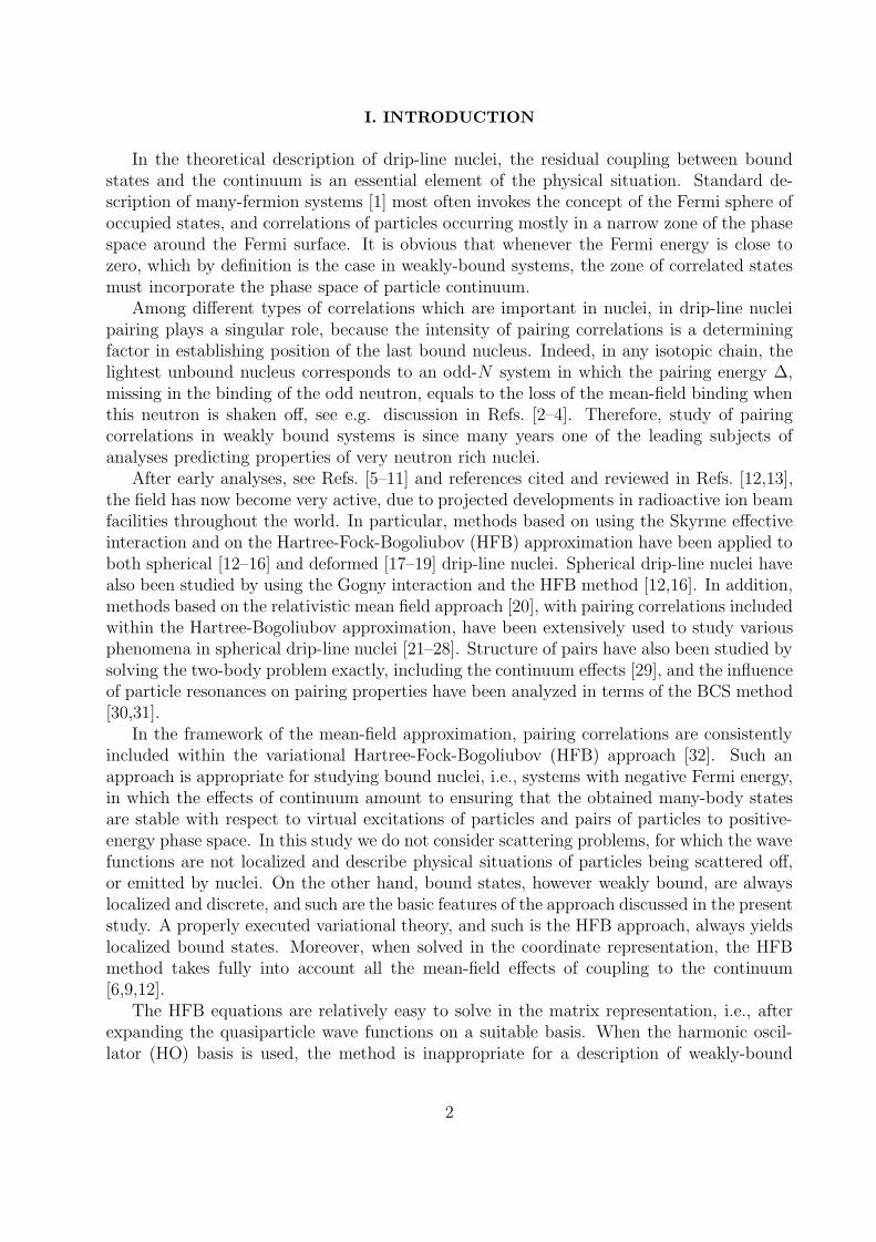
Unfortunately, in such a case the analytical solutions do not exist.For small values of Λ, the PTG potential is wide and diffuse. In Fig. 1 (lower panel)

we present the PTG potentials for L=0 and Λ=1, 3, and 7, with parameters s and νLj

(Table VII) chosen in such a way as to keep the depth and radius of the potential fixed. ForΛ = 1 and `=0 (see Fig. 1), one obtains the Poschl-Teller potential [45,46] which has beenwidely studied, e.g., in the molecular physics. For larger values of Λ, the PTG potentialgets steeper and resembles the Woods-Saxon potential. For relatively large values of Λ andrelatively small values of the depth parameter, one may find a small barrier at the edge ofthe potential well. Finally, for still larger Λ, the PTG potential resembles the finite-depthsquare well potential. The PTG potentials presented in Fig. 1 for Λ=3 and 7 correspond tothe profiles which are interesting from the point of view of simulating the nuclear mean fieldwithin a physical range of the diffuseness.

In the middle panel of Fig. 1 we present the L=4 radial PTG potentials, again forΛ=1, 3, and 7, and parameters s and νLj given in Table VII. Similarly, the top panel(with the corresponding parameters s and ν ′Lj) shows the L=4 potentials for the PTGcentrifugal barrier s2c(R) replaced by the physical centrifugal barrier. One can see that upto a little beyond the minimum, the PTG potential reproduces fairly well the potential withthe physical barrier. However, at larger distances, the PTG centrifugal term disappears tooquickly.

5

Nature of the energy eigenstates inside the potential well, as well as the nature of scat-tering solutions, depend strongly on the shape parameter Λ. The smaller is the value of Λ,the broader are the single-particle resonances. Below the critical value of Λcrit =

√2, the

resonances entirely disappear, i.e., there are no single-particle resonant states in any partialwave anymore.

III. RESONANCES

In this study we are interested in properties of the single-particle or quasiparticle reso-nances in the nuclear average potential. Quantum mechanics deals with numerous types ofquasi-stationary states. These states may be classified by the singularities of S-matrix or bythe mechanism of their production. One-particle shape resonances are perhaps the simplestlong-lived states. The particle is captured via quantum tunneling effect to the strongly at-tractive inner region of the potential. In this way, a quasi-stationary state is formed which,again through the tunneling effect, may leave this inner region. Similar in nature to the one-particle shape resonances are the one-particle virtual states. For these states, the confiningbarrier is absent but the potential exhibits large jump at the potential boundary regionwhich, in turn, causes jump in the particle wavelength. As a result, the quasi-stationarystate is formed, which slowly penetrates from inner to outer region of the potential. Theone-particle shape resonances and the one-particle virtual states are specifically quantumphenomena which have no counterpart in the classical physics.

Another kind of resonance states, the so-called Feshbach resonances, are formed whenincoming particle excites many particles in the parent nucleus and is captured in the inter-mediate state for which direct decay channels are closed. The decay of this state is thenproceeding through the series of de-excitations of a parent system to either initial channelor to the state of a total system having a lower positive energy [52]. Detailed microscopictheory of these resonances have been worked out in the case, when the coupling of inner exci-tation to decay channels is weak [53,54]. This has lead to the formulation of continuum shellmodel (CSM) [54] and to the description, e.g., of giant resonances as quasi-bound N -particlestates embedded in the continuum [55,56]. The CSM was extended recently to the realis-tic multi-configurational shell model which describes the coupling between the many bodywave functions for bound states and the one-particle scattering continuum. This so-calledShell Model Embedded in the Continuum (SMEC), allows for a simultaneous descriptionnot only of the shell model bound states and resonances but also of the radiative capturecross-sections [57,58].

Another type of many-channel quasi-stationary states may result due to the near-threshold singularity [59,60]. This can happen if the overlap of wave function in a givenchannel with other channel wave functions is small, leading to the effective decrease of thechannel-channel coupling and, hence, to the long lifetime. This resonance mechanism iscommon in the CSM [54,57].

Three-particle, near-threshold long-lived states constitute another class of resonancestates which is particularly interesting in the context of drip-line physics. In this class, bothnear-threshold virtual states (S-matrix poles at negative energies on nonphysical sheets) andresonance states (S-matrix poles in the complex plane) can be formed. Long-lived statesof this class are possible if there exists near-threshold bound, virtual or resonance state in

6

the two-particle subsystem. Multiple transitions of particles between these states of two-particle subsystem are leading to the appearance of effective, long-range exchange forcesin the three-particle system [61–63]. An analogous exchange process is also possible in thefour-particle systems [64]. The above recollection of most common resonance phenomena innuclear physics is by no means exhaustive.

A. Resonances as poles of the S-matrix

In the present Section we recall the standard theory of the S-matrix and introducethe so-called virtual states, which may appear in the single-particle phase space for smallenergies, and therefore are important for the discussion of pairing correlations in weaklybound systems, see Sec. V.

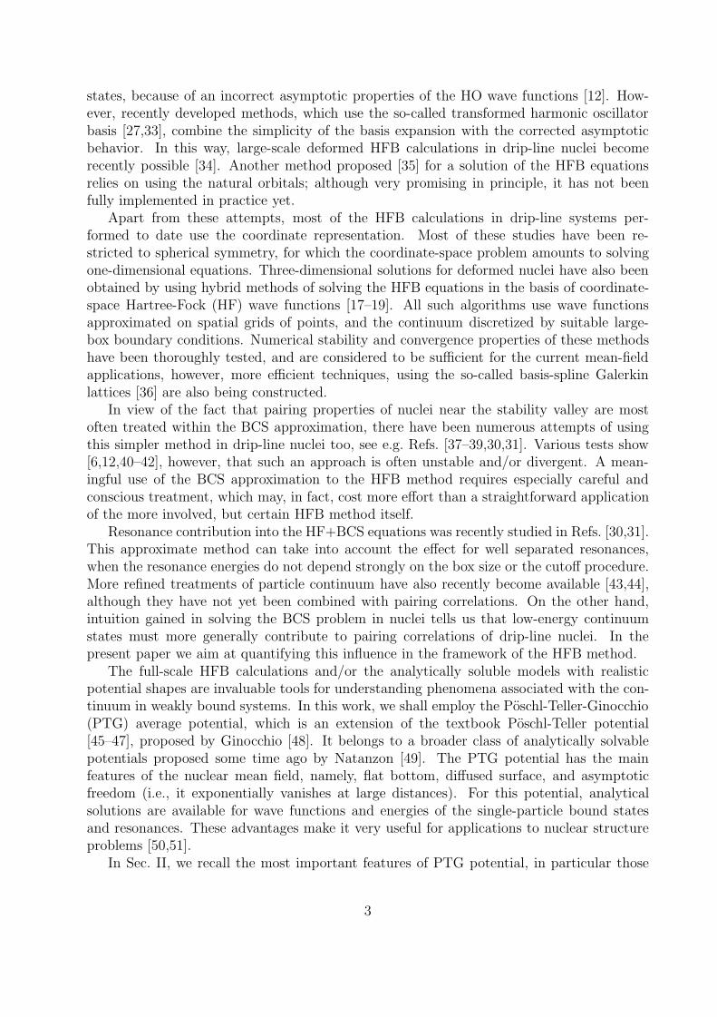
Poles of the S-matrix can be located in four different regions of the complex k-plane,corresponding to four regions of the two-sheet complex energy surface [65] (see Fig. 2).The position of a pole determines both the behavior of the respective wave function and thephysical interpretation of the solution. The first region corresponds to the positive imaginaryk-axis. The wave functions in this region are normalizable, negative energy solutions ofthe Schrodinger equation and correspond to the bound states of the system. The secondregion is the negative imaginary k-axis. Here solutions of the Schrodinger equation are notnormalizable (they are exponentially diverging) and, hence, they are not physical. Thesesolutions correspond to negative energies on the unphysical sheet of the energy surface andthey are said to be virtual or antibound (see Fig. 2c). The third region is the sector betweenthe positive, real k-axis and the bisection of the fourth quadrant. Asymptotically, thesolutions in this region, which correspond to the resonant states with the complex energy,are oscillating and exponentially decreasing functions. The imaginary part of the energywhich is negative in this case, is interpreted as a width of the state. Finally, poles locatedin the remaining region of the complex k-plane, are also said to be virtual.

Figure 2a presents different regions of the complex k-plane where the poles of the S-matrix are located, and the corresponding regions on the two sheets of the energy surface(Figs. 2b and c). The two sheets are connected along the real positive semiaxis. The arrowsin Fig. 2 represent the movement of poles, which results from decreasing the depth of thepotential well. In the general case, the poles corresponding to a bound state and to anantibound state move pairwise and cross at a given point (denoted κ in Fig. 2a). For L 6= 0,this point is situated at the origin. For L = 0, κ can be found lower on the imaginary axisand the determination of its position is in general not trivial (see [65]). After the crossing,the two poles move pairwise on the lower part of the complex k-plane. One considers thatthey are associated with the resonance phenomenon, once the pole on the right half-plane hascrossed the dashed line: <(k) = −=(k) (see Fig. 2c)), so that one can interpret its complexenergy (<(ε) > 0, =(ε) < 0) as the energy and the width of a resonance, respectively.Such poles are situated on the unphysical energy sheet but the lower one can influence thepositive-energy solution on the real positive energy axis.

Let us now discuss how the poles of the S-matrix are related to the widths of resonances.For that, let us consider the short ranged potential V (R) which tends to zero sufficientlyfast when R → ∞. The asymptotic (R → ∞) solution of the Schrodinger equation can bewritten as:

7

Ψ(R→∞) = A(k) exp(−ikR) + B(k) exp(+ikR)

' exp(−ikR) + S(k) exp(+ikR). (3.1)

We will be interested in the poles of S(k) when A(k) vanishes and we shall consider onlythose poles which are embedded in the fourth quarter (<(k) > 0, =(k) < 0) of the complexk-plane, i.e., those which are associated with the resonance phenomenon. Near the isolatedith pole, S(k) can be written as:

d (lnS(k))

dk= − 1

k − ki

, (3.2)

where ki is the complex pole.The number of poles in the quarter <(k) > 0, =(k) < 0, can be found following the

residue theorem:

N =1

2πi

∮C∂ lnS(k)

∂kdk. (3.3)

Consequently,

∂N

∂k= (2πi)−1∂ lnS(k)

∂k. (3.4)

The density of states:

ρ =

(∂N

∂k

)(∂k

∂ε

)−1

, (3.5)

can be expressed then as follows:

ρ = (2πi)−1∂ lnS(k)

∂ε. (3.6)

Inserting (3.2) into (3.6), it is then easy to see that the level density has a local maximumwhenever:

k = <(ki) , i = 1, · · · , N (3.7)

The value of density at the maximum is:

ρ(k = <(ki)) = − 1

2π=(εi), (3.8)

and corresponds to the complex energy:

εi − εth =(hki)

2

2m, (3.9)

where εth is the threshold energy. The density peaks have the Lorentzian shape and thefull-width half-maximum of ith peak is given by:

8

Γi =1

πρ(k = <(ki))= −2=(εi). (3.10)

Following this simple example, we assume that the poles of S-matrix on nonphysicalenergy sheets near the real axis correspond to almost all resonance states. Unfortunately, thishighly plausible assertion remains only a hypothesis because the relation between resonancesand the S-matrix poles is not determined so rigorously as the correspondence between thebound states and the S-matrix poles on the real axis of the first energy sheet. To affirmthe correspondence between the observed resonances and the S-matrix poles on nonphysicalsheets, certain conditions should be satisfied. First of all, the potential has to be sufficientlyanalytic and has to fall-off sufficiently rapidly at R → ∞, so that the corresponding S-matrix can be safely continued to the unphysical sheets. These conditions are satisfied forthe PTG potential, though the examples of potentials where the analytic continuation inthe eigenvalue problem brings around the redundant solutions are known as well [66,67]. Ingeneral, it is safe to speak about the resonance phenomenon in practical problems if thewidth is not large, i.e., ΓnLj/εnLj < 1 or, in other words, if the distance of the resonancepole from the physical region is small. This latter condition, as we shall show in sect. IV, isnever satisfied in the PTG potential for low-lying, near threshold resonances.

IV. SINGLE-PARTICLE WAVE FUNCTIONS AND RESONANCES IN THEPOSCHL-TELLER-GINOCCHIO POTENTIAL

A. Analytical results

Following Ref. [48], we express solutions of the radial Schrodinger equation with the PTGpotential (2.1) as functions of the variable x:

x =1− (1 + Λ2)y2

1− (1− Λ2)y2, (4.1)

where y is a function of the radial coordinate R, given by Eqs. (2.4) and (2.5). In the variablex, the Schrodinger equation transforms into the Jacobi equation, and its general solutioncan be expressed by means of the hypergeometric function:

ΨkLj(R) = χL(R)(

1 + x

2

)β2

(4.2)

× F

(L+ 3

2+β+νLj

2,L+ 3

2+β−νLj

2, L+

3

2;1− x

2

)

where

χL(R) =s

12

R[1 + Λ2 − (1− Λ2x)]

14

(1− x

2

)L+12

. (4.3)

For a given complex momentum k, the wave function is specified by two dimensionlessparameters:

9

β = − ik

sΛ2 (4.4)

and

νLj =[(νLj +

1

2)2 + β2(1− Λ2)

] 12

. (4.5)

The bound states occur for parameters β defined by:

β = βnLj, (4.6)

where

Λ2βnLj =[(

2n+ L +3

2

)2

(1− Λ2)

+Λ2(νLj +1

2)2)] 1

2 −(

2n+ L +3

2

)(4.7)

and n ≥ 0. In this case, the hypergeometric function reduces to the Jacobi polynomial, andthe solution reads [48]:

ΨnLj = NnLj[1 + Λ2 − (1− Λ2)x]14

×(

1 + x

2

)βnLj2(

1− x

2

)L+12

P(L+ 1

2,βnLj)

n (x), (4.8)

where NnLj is a normalization factor, and the number of bound states is limited by conditionβnLj > 0, which ensures that the eigenfunctions vanish at the infinity.

The bound-state energies are given by

εnLj =h2s2

2mEnLj, (4.9)

where the dimensionless eigenenergies are

EnLj = −Λ4β2nLj . (4.10)

It can be seen from the above equation that the tail of a bound-state wave functions forη →∞,

ΨnLj(R) ∝ e−βnLjΛ2(η−η0), (4.11)

does not explicitly depend on L, i.e., there is no influence of centrifugal barrier on any partialwave.

If Λ2 > 2, the resonances will occur for integer n such that:

n >1

2[Λ(Λ2 − 2)−1/2(νLj +

1

2)− 1] (4.12)

The dimensionless resonance energy is then:

10

EnLj = (2n+ L+3

2)2(Λ2 − 2)− Λ2(νLj +

1

2)2, (4.13)

and the dimensionless resonance width is:

γnLj = 4(

2n+ L+3

2

)×[(2n+ L+

3

2)2(Λ2 − 1

)−Λ2

(νLj +

1

2

)2] 12

. (4.14)

In the limit: EnLj → 0, the resonance width is:

γnLj → γ(0)nLj = 4(2n+ L +

3

2)2, (4.15)

and, hence, the ratio: γnLj/EnLj → ∞, for all values of parameter Λ. For small EnLj, wehave:

γnLj

EnLj

=γ

(0)nLj

EnLj

+ 2− 4EnLj

γ(0)nLj

. (4.16)

This ratio depends strongly on Λ. For large (n, L), the quantities EnLj and γnLj are propor-tional to (2n+ L)2 and their ratio is:

γnLj

EnLj

= 4(Λ2 − 1)1/2

Λ2 − 2, (4.17)

i.e. γnLj/EnLj < 1 for Λ > (10 + 4√

5)1/2. Therefore, in our numerical examples we presentresults for Λ=3 and 7, which are the values on two sides of the limiting case defined by thewidths of resonances being equal to resonance energies.

Solutions in the continuum can be found by analytically continuing the eigenfunctionsfrom a discrete negative energy to positive continuous energy (see Eq. (4.2)). The solutionsobtained in this way are proportional to hypergeometric functions. Imposing the boundarycondition that an incoming wave has the momentum k, one can determine the scatteringfunction for each angular momentum [48]. Using the asymptotic behavior of the most generalsolution (4.2) one obtains the matrix elements of the S-matrix:

S(k) = (−1)L+1 exp(

2β[Λ2η0 + ln Λ])

× Γ[−β]Γ[(L + 32

+ β + νLj)/2]

Γ[β]Γ[(L+ 32− β + νLj)/2]

(4.18)

× Γ[(L+ 32

+ β − νLj)/2]

Γ[(L + 32− β − νLj)/2]

.

Expression (4.18) yields the matrix elements of S-matrix for the Schrodinger problemwith the PTG potential without any restrictions, i.e., (4.18) contains informations aboutall mathematical solutions, both physical and unphysical ones. The poles of the S-matrixin the variable k = isΛ2β, correspond to the remarkable solutions [65] depending on theasymptotic behavior of solutions.

11

B. Wave functions

In the following we aim at analyzing the influence of weakly bound states and low-energyresonances on pairing properties of nuclei near neutron drip lines. Therefore, knowing theanalytical solutions available for the PTG potential, we chose three sets of parameters suchthat the 3s1/2 state is either weakly bound, or virtual, or there is a low-lying resonance inthe s1/2 channel. These three physical situations can be achieved by fixing parameters Λand s and shifting the depth parameter νs 1

2. In the specific examples discussed below, we

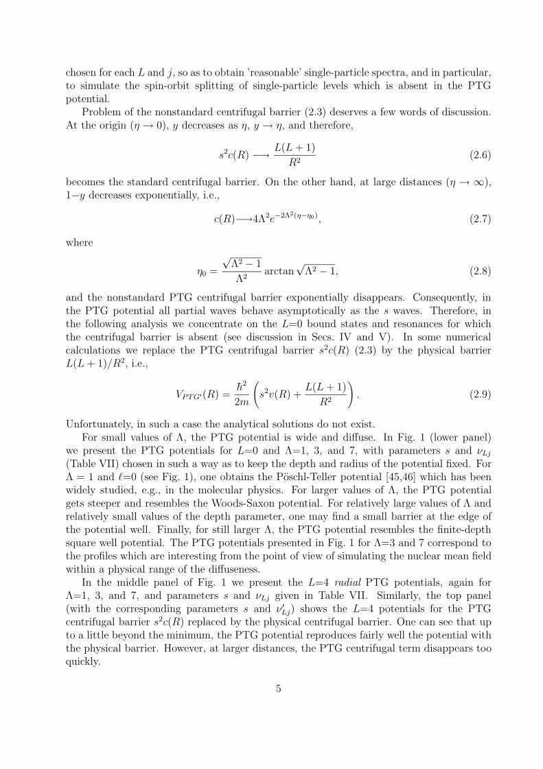
use the parameters listed in Table II, where also the corresponding energies are given.Wave functions of the resonant, virtual, and bound 3s1/2 states are shown in Fig. 3.

The resonant wave function is calculated at the energy equal to the real part of the poleshown in Table II. Normalizations of the virtual and resonant wave functions are chosenso as to match the height of the first maximum of the bound wave function. The threewave functions illustrate properties of single-particle phase space in the situation where the3s1/2 state leaves the realm of bound states, dwells for a short time in a ghost-like zone ofvirtual states, and then reappears as a decent (although very broad) resonance. From thepoint of view of the asymptotic properties, pertinent to the scattering problems, these threewave functions are completely different. On the other hand, from the point of view of theirstructure inside the nucleus (see the inset in Fig. 3), they are almost exactly identical. Infact, in the scale of the inset, the resonant wave function cannot be distinguished from thebound one.

In Sec. V we also study several cases of different positions of the 2d3/2 states. In particu-lar, we use two values of the depth parameter νd 3

2, which are listed in Table II together with

the corresponding energies of the 2d3/2 PTG resonance and virtual states. Whenever thespectrum in all partial waves is required, like in the HFB calculations below, we combineνd 3

2=4.900 with all the three values of νs 1

2, and νs 1

2=5.034 with all values of νd 3

2.

C. Localizations and phase shifts

Since the pairing potentials depend self-consistently on the pairing densities, they areconcentrated inside the nucleus, i.e., they are nonzero inside, and go to zero outside thenuclear volume. Therefore, the more the continuum wave functions are concentrated insidethe nucleus, the more they are sensitive to the pairing coupling. In order to quantitativelycharacterize the wave functions from this point of view, we introduce their ’localization’ asthe norm inside the sphere of radius RLoc,

L [ψ] =∫ RLoc

0|ψ(r)|2 dr, (4.19)

where the radius RLoc is, for the purpose of the present study, arbitrarily fixed at RLoc =1.5 × R1/2 = 7.578 fm, while R1/2 is the radius where the potential drops to its half value.[Note that the volume element 4πr2 is included in the definition of wave function ψ(r).] Forthe bound states, localization is just the probability to find the particle inside the sphereR<RLoc. For the continuum wave functions which are not normalizable, localization dependson the chosen normalization condition.

12

Below we present results for the continuum wave functions normalized in two ways.Firstly, we may normalize them to unity inside the box of a large radius. (The value ofRbox=30 fm is chosen for all results obtained in the present study.) Outside the box, thewave functions oscillate and have an infinite norm. In this case, the localization is a fractionof the probability to find the particle inside the nucleus relative to the probability to find itinside the box. Absolute values of such a localization depend, of course, on the radius of thebox, however, we are only interested in comparing relative localizations of the wave functionswith different energies. Secondly, we may normalize the continuum wave functions in sucha way that they all have a common arbitrary amplitude in the asymptotic region. For wavefunctions in which the volume element 4πr2 is included, as is the case here, their amplitudesdo not asymptotically depend on r. Again, the absolute values of this localization dependon the value of the common amplitude, but the relative values tell us at which energy thegiven wave function is better concentrated inside the nuclear volume. One may chose othernormalization conditions (to a delta function in energy or in momentum, for example), butwe did not find any advantage in looking at the corresponding localizations, and we discusshere only the two ways described above.

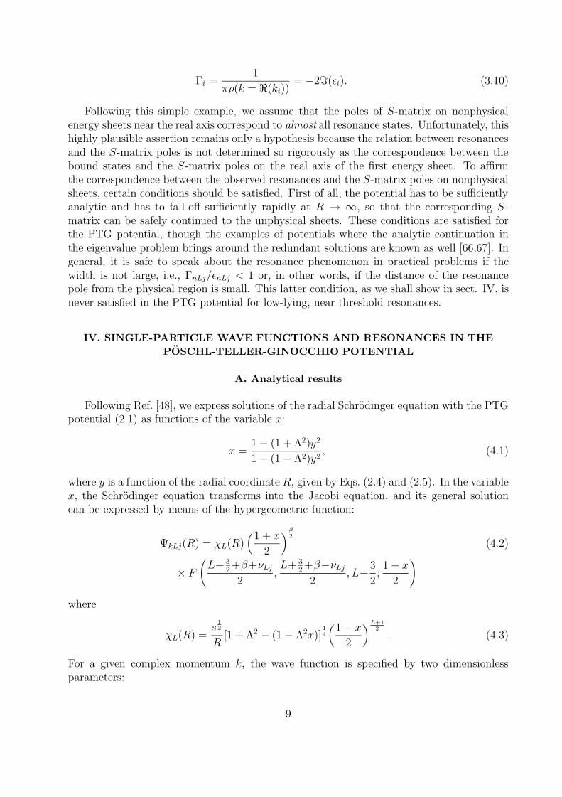
Fig. 4a shows values of localizations of the s1/2 PTG continuum states, calculated ana-lytically, for the normalization in the box (solid line) and for the normalization to a constantamplitude (dashed line). Calculations are performed for the PTG potential for which thereis a weakly bound 3s1/2 state (cf. Table II), and therefore, the lowest resonance in thes1/2 channel appears high in energy. The wide bump in the localization, which is seen near40 MeV reflects the known fact that the S-matrix pole at (39−18i) MeV generates continuumstates which are more localized than the continuum states far from the resonant energies.However, values of localizations near the maximum are only a factor of 2-3 larger than thosefar from the maximum, i.e., one cannot a priori expect that the only continuum states whichcan couple to the pairing field are those close to resonances.

One can see that the localization obtained from normalizing the continuum states in thebox (solid line) presents numerous wiggles, which appear when the consecutive half-wavesenter the box. On the other hand, the localization obtained from the amplitude normaliza-tion is given by a smooth curve. Both localizations are fairly similar, and therefore, differentnormalization prescriptions do not affect our conclusion about the relative localizations ofthe continuum states.

There is some difference between these two different normalization prescriptions whenε→0. At the origin, φ(r)=A sin(kR). In case of the normalization in the box, we can assumefor k→0 that this expression is valid in the whole box. Then :

∫RLoc0 φ2(r)dr/

∫R0 φ2(r)dr '∫RLoc

0 r2dr/∫R0 r2dr = (RLoc/R)3 = const. We have verified this assertion also numerically. In

the case of normalizing to an amplitude A, for k→0 one gets:∫RLoc0 φ2(r)dr ' |A|2k2r3/3 −→

0. Therefore, the dashed curve turns sharply down when approaching ε=0.In Fig. 4a we also present localizations of the continuum states calculated numerically

(circles) in the same box of Rbox=30 fm, and using the discretization of wave functions ona mesh of nodes equally spaced by H=0.25 fm. One can see that the numerical resultsperfectly reproduce the analytical calculations for the same normalization. In the numer-ical calculations, the box plays merely a role of selecting from the infinite continuous setof positive-energy solutions a discrete subset of wave functions which vanish at the boxboundary. Apart from that, the numerically calculated wave functions are very precise

13

representations of the exact wave functions for some specific discretized values of the energy.Fig. 4b shows the phase shifts of the same continuum states calculated analytically

(solid line) and numerically (circles). (In this case, normalization of the continuum wavefunctions does not play any role.) Again, one can see that the numerical results very preciselyreproduce the analytical ones in the whole range of studied energies.

Usually, one identifies the resonance when the phase shift passes π/2 (or better nπ/2,as the phase shift is defined modulo 2π). This definition works well for narrow, well sepa-rated resonances. In the case of PTG potential, the resonances are broad and this definitionis inadequate. It is then better to identify the resonance with the inflection point in thederivative dδ(ε)/dε. This also demonstrates real difficulty in identifying resonances in po-tentials with diffuse surfaces and proves again the advantage of the soluble models wherethe S-matrix is analytically known and the poles can be analytically studied.

V. PAIRING IN WEAKLY BOUND SYSTEMS

A variational mean-field approach to pairing correlations results in the HFB equations[32]. In weakly bound systems, these equations should be solved in coordinate space inorder to properly take into account the closeness of the particle continuum [6,12]. In themost general non-local coordinate representation, the HFB equations have the form of thefollowing matrix integral eigenequation:

∫d3r′∑

σ′

(h(rσ, r′σ′) h(rσ, r′σ′)h(rσ, r′σ′) −h(rσ, r′σ′)

)(φ1(E, r

′σ′)φ2(E, r

′σ′)

)

=

(E + λ 0

0 E − λ

)(φ1(E, rσ)φ2(E, rσ)

), (5.1)

where E is the quasiparticle energy, λ is the Fermi energy, and h(rσ, r′σ′) and h(rσ, r′σ′)are the mean-field particle-hole (p-h) and particle-particle (p-p) Hamiltonians, respectively.Contrary to the HF equations, which define one-component (single-particle) wave functions[the eigenstates of h(rσ, r′σ′)], the HFB method gives two-component (quasiparticle) wavefunctions (the upper and lower components are denoted by φ1(E, rσ) and φ2(E, rσ), respec-tively).

In the following, we solve the HFB equations (5.1) by fixing the p-h Hamiltonian to beequal to the sum of the kinetic energy (with constant nucleon mass) and PTG’ potential(2.9). In this way, we study self-consistency only in the pairing channel, while the single-particle properties are kept unchanged, and under control. For example, the single-particleenergies and resonances do not change during the HFB iteration, and are not affected bythe pairing properties, which would have not been the case had we allowed the usual HFBcoupling of the p-h and p-p channels. Moreover, within such an approach we only need tosolve the HFB equations for neutrons, i.e., for the particles which exhibit the weak bindingunder study here. Note that for the physical centrifugal barrier included in all the L>0partial waves, the energies of single-particle bound states and resonances are not given byanalytical expressions (4.10) and (4.13). However, the barrier does not appear in the s1/2

channel, and these energies are still given analytically.

14

Two parameters of the PTG potential have been fixed at values used in the previousSections, namely, Λ=7 and s=0.04059, while the depths parameters νLj (Tables II and III)have been chosen in such a way [48] as to simulate a hypothetical single-particle neutronspectrum in drip-line nuclei with N<∼82. For the scope of the present study, details of thisspectrum are insignificant; we only aim at realizing the physical situation where the PTG’3s1/2 or 2d3/2 states are near the threshold (close to zero binding energy) and at the sametime the Fermi energy is negative and small.

Contrary to the p-h channel, the full self-consistency is required in the p-p channel, withthe p-p Hamiltonian given by the local pairing potential [6,12]:

h(rσ, r′σ′) = U(r)δ(r − r′)δσ,σ′ , (5.2)

where

U(r) =1

2V0ρ(r), (5.3)

and

ρ = − ∑0<En<Emax

∑σ

φ2(En, rσ)φ∗1(En, rσ). (5.4)

Potential (5.3) corresponds to the pairing force given by the zero-range interaction,

V (r1 − r2) = V0δ(r1 − r2). (5.5)

Strength parameter V0 has been arbitrarily fixed at V0=−175 MeV fm3. The pairing phasespace, given by the cut-off parameter Emax, has been fixed according to the prescriptionformulated in Ref. [6]. In Eq. (5.4) we used the fact that in order to discretize the contin-uum HFB states, the HFB equation is solved in a suitable spatial box. The HFB resultspresented below have been obtained with the same box size of Rbox=30 fm as those discussedin Sec. IV C.

As seen from Eqs. (5.1)–(5.3), the intensity of the pairing coupling [i.e., the off-diagonalterm in Eq. (5.1)] is given by the integral of the wave functions with the pairing densityρ(r). This integral can be approximated in the following way:∫

d3r∑σ

φ∗1(En, rσ)ρ(r)φ2(En, rσ) ' ρ0 (NnL[φ∗1])1/2 , (5.6)

where L[φ∗1] is the localization of the upper HFB wave function, defined as in Eq. (4.19),and Nn is the norm of the lower HFB wave function:

Nn =∫

d3r∑σ

|φ2(En, rσ)|2. (5.7)

Equation (5.6) gives only a very crude approximation, which aims only at showing themain trends. It is based on two assumptions: (i) that the pairing potential is constant withinthe radius RLoc of the sphere for which the localization is defined, and zero otherwise. Zero-range pairing force (5.5) leads to the volume-type pairing correlations [12], for which thepairing densities are spread throughout the nucleus, and can be crudely approximated by a

15

constant value ρ0. Another assumption is: (ii) that the lower and upper HFB wave functionsare proportional to one another within the radius of RLoc. We know that this assumptionholds only in the BCS approximation, while in the HFB approach the lower and uppercomponents are different, including different nodal structure [12]. For all energies En, thelower components are localized inside the nucleus, and their norms Nn give contributionsto the particle number (see examples of numerical values presented in Ref. [12] and inthe following subsections). On the other hand, the continuum upper HFB wave functionsbehave asymptotically as plane waves, however, their pairing coupling is dictated by theirlocalizations. We are not going to use Eq. (5.6) in any quantitative way; we only use itas a motivation to look at localizations of the upper HFB components as measures of howstrongly given continuum states contribute to pairing correlations.

A. The s1/2 continuum

Figures 5 and 6 show the s1/2 localizations and phase shifts, respectively, of the upperHFB quasiparticle wave functions calculated numerically (dots), compared with the analyti-cally calculated localizations and phase shifts of the PTG states (lines). We are interested inthe low-energy s1/2 continuum, and therefore the Figures show results well below the broad(39−18i) MeV resonance discussed in Sec. IV C. The PTG results (no pairing) are shownas functions of the single-particle energy ε, while the HFB results are plotted as functionsof the quasiparticle energy E shifted by the Fermi energy λ, i.e., E+λ. In this way, at largeenergies the paired and unpaired energy scales coincide.

Three panels presented in Figs. 5 and 6 correspond to the PTG 3s1/2 states being resonant(a), virtual (b), and weakly bound (c), cf. Table II. In order to realize these three differentphysical situations, the bottom of the PTG potential has to be shifted by about 2.75 MeV.This illustrates the “width” of the zone where the 3s1/2 states are virtual. Apparent shiftin the single-particle energies is much smaller; the 3s1/2 state moves then from the −74 keVbound-state energy to the 74 keV resonance energy (Table II). Even if the shift in thesingle-particle states is so small, the corresponding canonical states move by about 1.75 MeV(Table IV). These latter states appear to be entirely unaffected by the dramatically differentcharacter of the single-particle 3s1/2 states (Fig. 3). Their wave functions, shown in Fig. 7,are almost identical in the three cases (a)-(c).

Since the canonical states govern the pairing properties of the system, see discussion inRef. [32], their positions explain the changes in the overall pairing intensity 〈∆N〉, and in the3s1/2 occupation v2

can, shown in Table IV. It is worth noting that shifting the canonical 3s1/2

level from its ∼0.8 MeV distance to the Fermi level to a distance of ∼2.5 MeV decreases theaverage pairing gap by as much as about 300 keV.

Apart from the decrease of the pairing intensity described above, there is no other qual-itative change in pairing properties when the 3s1/2 state becomes unbound. The role ofthe weakly bound state is simply taken over by the low-energy continuum. The presenceand position of the low-energy s1/2 resonance is not essential for the pairing properties. Inparticular, it would have been entirely inappropriate to use this resonance, and its energyof 74 keV, in any approximate scheme in which the full continuum was replaced by theresonances only.

16

In all the three cases (a)-(c), in the region of energies between 10 and 20 MeV (Fig. 5)one can see the “background” localization of the order of 0.2. These energies are far awayfrom resonances, and therefore illustrate localizations of a “typical” non-resonant continuum.Near the resonances (see Figs. 4a and 5a), localizations are larger, up to 0.3, but do not atall dominate over the background value. Therefore, based on estimate (5.6) one may expectthat the pairing coupling of the resonant and non-resonant s1/2 continuum is fairly similar.

The magnitude of this coupling seems to depend primarily on the s1/2 single-particlelocalization in the 2–3 MeV zone above the Fermi surface. (Note that cases (a)-(c) differonly by positions of the s1/2 states; the spectra in other partial waves are kept unchanged.)The weakly bound 3s1/2 PTG state generates large continuum localization right above thethreshold, and the opposite is true for the low-lying 3s1/2 PTG resonance. Therefore, theaverage pairing gap 〈∆N〉 is substantially larger in case (c) than in case (a), and as aconsequence, the HFB localizations in case (c) differ strongly from the PTG localizations,while in case (a) they are almost identical. The same pattern clearly also appears for theHFB phase shifts, as compared to the PTG phase shifts, Fig. 6.

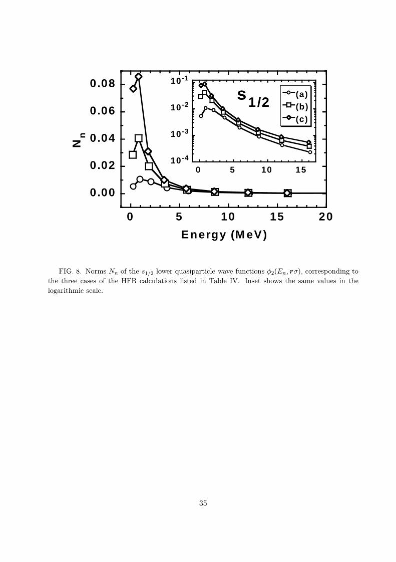
Figure 8 shows norms Nn of the lower HFB components, Eq. (5.7). Since the lower HFBcomponents are not mutually orthogonal, Nn cannot be associated with the occupationprobabilities. On the other hand, the canonical occupation factors v2

can do play such a role,because the canonical states form an orthogonal basis. Comparing values of Nn (Fig. 8) andv2can (Table IV), one sees that the canonical 3s1/2 state collects all the occupation strength

of the quasiparticle states in the low-energy continuum. Of course, numbers Nn scale withthe overall pairing strength, i.e., they are smaller in case (c) than in case (a), but in everycase all quasiparticle states below about 5 MeV significantly contribute to v2

can. Moreover,choosing only one quasiparticle state in this zone (call it resonance or not), would haveprovided only for about one third of the occupation factor. This illustrates again that thes1/2 continuum has to be taken as a real continuum (discretized, if needed), and not throughany single representative.

B. The d3/2 continuum

Since the low-energy s1/2 resonances are always very broad, the distinction between theresonant and non-resonant continuum is not very clear in this channel. On the other hand,pairing coupling of very narrow high-j resonances is not very different from that of any otherbound states, and hence they are not very interesting to look at. Therefore, in addition toinvestigating the s1/2 resonances, we also study here an intermediate case of low-energy 2d3/2

resonances, which can be narrow or broad depending on their positions inside the centrifugalbarrier. For that we use the PTG’ potential which contains the physical centrifugal barrier,Eq. (2.9), and chose several different values of the depth parameter νd 3

2.

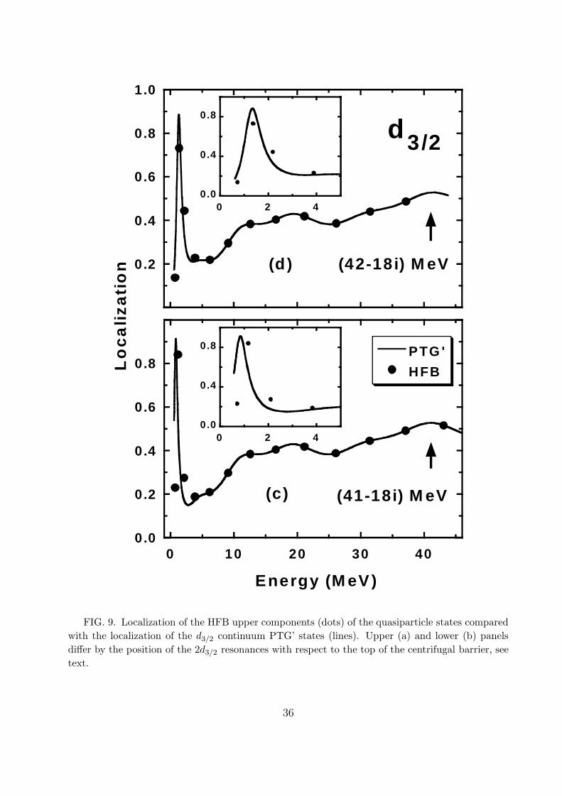
First, we study two cases listed in Table II, chosen in such a way that the resonancesare located at two different positions deep inside the centrifugal barrier. (For the chosendepths, in the PTG potential the 2d3/2 states are resonant (d) or virtual (e); their analyticalenergies are given in Table II.) Although for the physical barrier the analytical resultsare not available, one can estimate the resonance energies to be about εres'(1.5−0.4i) MeV(d) and εres'(0.9−0.2i) MeV (c), respectively. In the two cases, the resonances are locatedat about 3.5 MeV and 4.1 MeV below the top of the barrier which is about 5 MeV high.

17

One can see that the inclusion of the physical barrier moves the PTG resonance (Table II)up in energy and decreases its width by a factor of eight, while the PTG virtual state istransformed into a true, rather narrow resonance.

Figure 9 shows the HFB and PTG’ localizations of the d3/2 continuum states. Of course,the low-energy PTG’ resonances create narrow peaks of localizations at the resonant energies,and having resonance widths. Insets in Fig. 9 show that the pairing correlations shift thePTG’ localizations to slightly higher energies, but otherwise the HFB and PTG’ localizationsare very similar. Beyond the narrow resonances, the HFB and PTG’ localizations reach thenon-resonant background values of about 0.3–0.4, which are almost unaffected by the next,very broad d3/2 resonance at about 40 MeV.

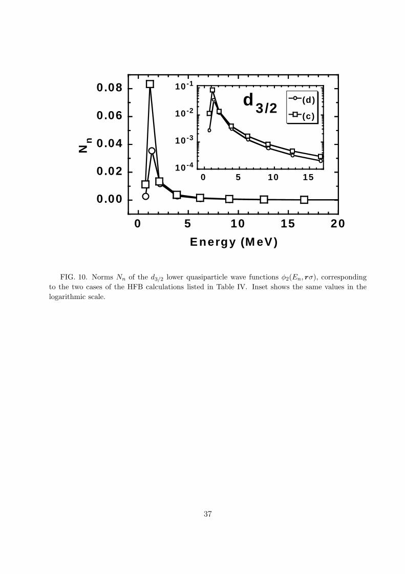
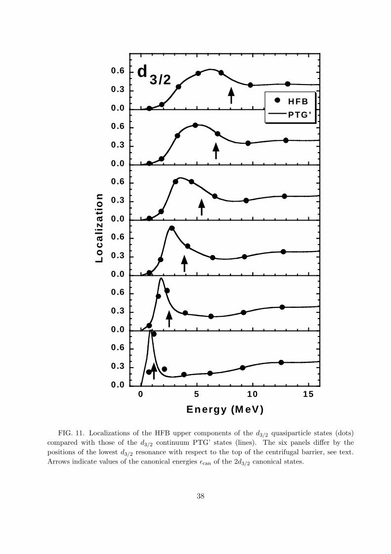
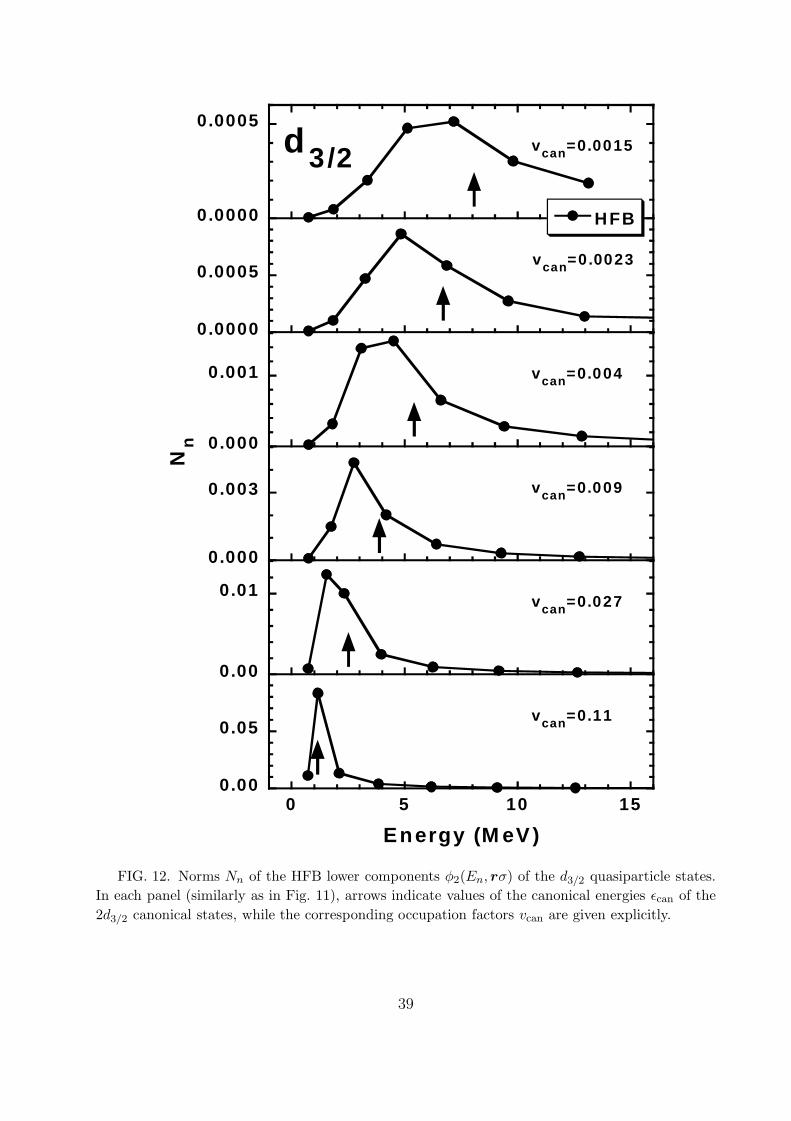
Apart from the change in overall pairing intensity, see Table IV, norms of the lowerHFB components Nn shown in Fig. 10 closely follow the shape of localizations. In orderto further visualize this property, in Figs. 11 and 12 we show results corresponding to the2d3/2 resonances when they are moved up to the top of the centrifugal barrier. Six panelspresented in the Figures have been obtained by using the depth parameters νd 3

2=4.9(0.1)4.4,

which corresponds to shifting the bottom of the d3/2 central potential well from −48.4 to−39.8 MeV. As a result, the 2d3/2 resonances move from about 0.9 MeV to 6 MeV (at thesame time the barrier also slightly increases, from 5 to 6 MeV). Hence, the top panels inFigs. 11 and 12 correspond to a broad resonance located right at the top of the centrifugalbarrier.

Localizations of the PTG’ d3/2 continuum states (Fig. 11) closely follow the patternof broadening and rising resonances. Apart from the lowest two panels, corresponding tolow-energy resonances, the HFB localizations (dots) do not differ from the PTG’ results(lines). This is because the larger the distance of the resonance from the Fermi surface(λN'−0.4 keV in all cases), the weaker are, of course, modifications induced by pairingcorrelations. Moreover, the rising resonance leaves behind (at low energies) very low values oflocalizations, which additionally contributes to a decreasing of the overall pairing intensities.

Interestingly, norms of the lower HFB components Nn, presented in Fig. 12, closely followthe pattern of localizations. It means that values of localizations of the PTG’ single-particlestates indeed decide about the pairing coupling of the HFB quasiparticle continuum states,cf. Eq. (5.6). However, again none of the quasiparticle states (close to resonant energiesor not) can be used as a single representative of the continuum phase space. Even for theresonances located very deeply inside the barrier (the lowest panels in Fig. 12), norms Nn

for quasiparticle states at resonance energies do not exhaust the occupation numbers vcan.In Figs. 11 and 12, arrows indicate values of the canonical 2d3/2 energies εcan. With

resonances moving up, these energies increase too, and appear always slightly above theresonant energy. These canonical states represent correctly the whole region of the quasi-particle continuum within, and above the centrifugal barrier. The 1d3/2 canonical states aredeeply bound (∼−25 MeV), and the 3d3/2 canonical states are very high (∼+25 MeV), soindeed those corresponding to 2d3/2 (as shown in the Figures) are well separated represen-tatives of a wide region of the phase space. Therefore, any approximate scheme, aiming ata correct description of pairing correlations near continuum, should vie to find these statesat right places. Unfortunately, the HF+BCS method which uses resonant continuum statesonly, does not seem to have a chance to attain such a goal. However, similarity of localiza-tions and norms Nn found in the present study may give hope for approximate solutions of

18

HFB equations. Of course, when the spherical symmetry is conserved, direct solution of theHFB problem is easy enough that no approximated methods are necessary. However, this isnot the case for the deformed systems, where moreover, single-particle resonances split andbecome much more difficult to treat.

VI. PERSPECTIVES AND OUTLOOK

The states at positive energies having maximum localization inside the region of potentialwell, preserve a remnant of the eigenvalue structure [68,69]. Whether virtual or resonant,these low lying states are likely to play an important role in the low-energy phenomena.For example, the neutron direct radiative capture process, which depends on propertiesof nuclear potential both at the surface and in the interior regions, is a unique tool toinvestigate properties of nuclear wave functions. Similar information may also be derivedfrom the inverse process, i.e., the Coulomb dissociation process, and both those processes aregoing to be very important in extracting the information about nuclei close to the drip line.Raman et al. [70] have shown how strongly the details of a neutron-nucleus potential affectthe capture mechanism for s-neutrons. (Extension of this analysis to higher partial waveshas been done recently by Mengoni et al. [71].) This is also important in many astrophysicalissues, e.g., the inhomogeneous Big Bang model or the neutron poison problem.

Low-lying resonant states may influence the pairing correlations enhancing the bindingenergy of halo nucleons (neutrons). In this work we have seen that a presence near thresholdof the L=0 poles of the S-matrix corresponding to bound, virtual, and resonance states, mayinfluence the pairing correlations and increase the localization of scattering wave functionsin the narrow range of ∆ε '2–4 MeV above the threshold. Hence, the pairing interactioninduces a subtle rearrangement effect in the structure of scattering states which modifiesthe strength of pairing field and the binding energy of affected nucleons close to the Fermisurface what, in turn induces new rearrangement in the structure of low lying scatteringstates, etc. This effect can be described only in the self-consistent treatment of pairingcorrelations.

For the HF potentials where the resonance width Γ tends to a finite value when theresonance energy ε tends to zero, in the physical situation corresponding to the drip lines,i.e., when the nucleon (neutron) separation energy tends to zero (Sn → 0), and hence−λn−∆ '0, the standard quasiparticle picture [72] may be questionable. For the quasipar-ticle picture to be valid, the appreciable fraction of the single-particle strength should remainin the quasiparticle excitations and, moreover, the lifetime of excitations about the Fermisurface should be relatively long. Whether the single-particle strength is concentrated inthe quasiparticle excitations depends on the strength of the residual interaction mixing thesingle-particle strength into more complicated configurations. But even when the residualinteraction is strong, one can always assure in normal systems that the quasiparticle lifetimeis long, i.e., the spreading of the quasiparticle strength function is small. In those systems,width of a quasiparticle state Γ(k) ∼ (k − kF )2 can be made small by letting k approachkF [73]. This result is independent of details of the interaction and follows from the Pauliprinciple and the phase-space considerations. However, as demonstrated in the example ofthe PTG potential, the states above the Fermi surface of kF'0 may have a finite width inthe limit of k → kF . In spite of the fact that the PTG centrifugal barrier is different from

19

the physical centrifugal barrier, this feature should be seen in the structure of weakly boundnuclei near the drip line, at least for systems where L=0 states are present near threshold.

This particular aspect does not seem to be modified by including the pairing correlationswithin the HFB method. Consequently, the perturbation theory may not be applicablein these systems, and various kinds of instabilities caused by the residual correlations areexpected. These instabilities may change the initial HF(B) vacuum in these nuclei non-perturbatively. In other words, one may expect that the spectrum of excitations in theunperturbed HF(B) system may not be compatible with the spectrum of excitations in theHF(B) system perturbed by the residual correlations. This brings about a new and challeng-ing aspect into the experimental studies of shell structure and excitations close to the dripline: The atomic nuclei at the drip-line may provide a new kind of quantum open systemwith yet unknown properties of its excitation spectrum, resulting from the strong couplingbetween bound interior states and the environment of scattering states. If discovered, itsmicroscopic description may call for new techniques in solving the quantum many-bodyproblem. Similar coupling between the localized quasi-stationary states and the scatteringstates has already been recognized to be responsible for the unusual features of the surfaceof nuclear potential [58].

One of the most interesting aspects of correlations in drip-line systems is the questionof multipole instabilities and deformations. A basis to study such phenomena should beprovided by including the HFB pairing correlations in deformed states. This is a verydifficult task, and only recently first attempts of such solutions become available [17,18,34].The problem here is related to solving the HFB equations in a deformed coordinate-spacerepresentation, in a situation where variational methods are not applicable because theHFB equation has a spectrum unbounded from below. However, in our opinion, only suchan approach may provide a sound basis of quasiparticle states in which other correlations(perturbative or not) may further be investigated.

It is essential to distinguish between five different aspects of the pairing coupling to thecontinuum phase space. First, enough continuum has to be included to cover the zone aroundthe Fermi level, which is reasonably larger than the pairing gap. For gaps of about 1 MeVthe zone which is 5 MeV wide is often used, cf. Ref. [17]. Second, the low-lying continuumwith large localizations has to be taken into account. In cases studied here (Fig. 5), thezone of 5 MeV seems to be enough, however, this aspect strongly depends on the shape anddepth of the single-particle potential, and the safe limit should probably be at least twicelarger. Third, enough continuum should be included so as the contributions Nn to particlenumber become small, and quasiparticle states entering and leaving this zone do not causesignificant changes. A limit of Nn'0.001–0.0001 is probably the least one can get away with,which already requires going up to 10-15 MeV into the continuum, see Fig. 8. Fourth, allquasiparticle states which significantly contribute to the canonical states (i.e., those whichhave large spectral amplitudes [12]) should be included, which requires 10-20 MeV of thecontinuum [12]. Finally, a coupling between particle-type and hole-type quasiparticle stateshas to be taken into account. Although this coupling is not responsible for the physicalwidths of deep hole states, cf. discussion in Ref. [12], it is present in the HFB equations, andaffects continuum solutions. This aspect requires taking continuum up to energies exceedingthe depth of the single-particle potential, i.e., to about 40-50 MeV, and such a prescription [6]has been used here. Needless to say that the above discussion concerns the HFB continuum;

20

analyses based on the BCS method, which use the single-particle continuum, have otherproperties, and often diverge with increasing continuum cut-off energy.

VII. CONCLUSIONS

Much is known about the analytic properties of one-particle wave functions in the lowenergy continuous spectrum when there is a real, virtual or quasistationary level with energyclose to zero [68,69]. It was shown for a number of potentials, that the continuum wavefunctions in a wide range of r-values have the r-dependence which is remarkably close tothat of the wave function for the zero-energy level [74,68,69]. Validity of this finding has beenalso discussed in Sec. IV B (see Fig. 3). As noticed by Migdal et al. [68], this approximatefactorization of the continuum wave functions in the resonance region of one-particle phasespace should simplify the computation of matrix elements. In the HF+BCS approach ofRefs. [30,31], it is assumed that the analytical features of the S-matrix, which lead to thefactorization property of the single-particle wave functions in the resonance region, remainvalid in the presence of pairing correlations. Actually, this weak perturbation hypothesis forthe S-matrix in the presence of pairing interaction remains not proved. To which extendthe structure of single-particle resonances and the non-resonant continuum is affected by thepresence of short-ranged correlations of the pairing type is the main problem which we haveaddressed in this work using the two-component quasiparticle wave-functions of the HFBapproach and the PTG single-particle potential for which the S-matrix properties are knownanalytically. The detailed analysis performed in this work, shows that this weak perturbationassumption for the analytic structure of the S-matrix for the one-particle problem may behazardous in many situations.

The comparison of the localization of HFB upper component of the quasiparticle stateswith the localization of the s1/2 continuum PTG states exposed a complicate interplaybetween resonant and non-resonant HFB continuum which by no means can be approximatedby the HF+BCS approximation spanned on the skeleton of the S-matrix resonances for theone-particle problem. The energy position of canonical states, which govern the pairingproperties of the system, is not correlated with the presence and position of pole in theS-matrix for the one-particle problem. As a consequence, the pairing coupling of resonantand non-resonant s1/2 continuum is quite similar, and its magnitude depends on the single-particle localization in the interval of 2–3 MeV above the Fermi surface.

When the single-particle poles are very close to the real axis in the momentum space(<(k) > 0), like in the case of very narrow high-j resonances deep inside the centrifugalbarrier, the pairing interaction is too weak to perturb the single-particle pole structure and,hence, these resonances are not very different from the bound states.

In the intermediate case, like d3/2-resonances studied in Sec. V B, the situation dependson the position of the single-particle resonance with respect to the top of the centrifugalbarrier. In a typical case, however, norms of the lower HFB components closely follow thepattern of localizations in the corresponding single-particle continuum, i.e., localizations ofthe single-particle continuum states determine the strength of the pairing coupling of theHFB quasiparticle continuum. However, like for the s1/2 continuum, none of the quasiparticlestates can be used a as a single representative of the continuum phase space.

21

ACKNOWLEDGMENTS

This research was supported in part by the Polish Committee for Scientific Research(KBN) under Contract No. 2 P03B 040 14, by the U.S. Department of Energy under ContractNos. DE-FG02-96ER40963 (University of Tennessee), DE-FG05-87ER40361 (Joint Institutefor Heavy Ion Research), DE-AC05-96OR22464 with Lockheed Martin Energy ResearchCorp. (Oak Ridge National Laboratory), by the NATO grant CRG970196, by the French-Polish integrated actions programme POLONIUM, and by the computational grant fromthe Interdisciplinary Centre for Mathematical and Computational Modeling (ICM) of theWarsaw University. The authors wish to thank W. Nazarewicz for the hospitality extendedto them during the visit at ORNL where part of this work has been done and for the criticalreading of the manuscript.

22

REFERENCES

[1] A.B. Migdal, Theory of Finite Fermi Systems and Applications to Atomic Nuclei (In-terscience, New York, 1967).

[2] M. Beiner, H. Flocard, N. Van Giai, and P. Quentin, Nucl. Phys. A238, 29 (1975).[3] R. Smolanczuk and J. Dobaczewski, Phys. Rev. C48, R2166 (1993).[4] J. Dobaczewski, W. Nazarewicz, and T.R. Werner, Physica Scripta T56, 15 (1995).[5] A. Bulgac, Preprint FT-194-1980, Central Institute of Physics, Bucharest, 1980.[6] J. Dobaczewski, H. Flocard and J. Treiner, Nucl. Phys. A422, 103 (1984).[7] M.V. Zverev and E.E. Sapershteın, Sov. J. Nucl. Phys. 39, 878 (1984).[8] M.V. Zverev and E.E. Sapershteın, Sov. J. Nucl. Phys. 42, 683 (1985).[9] S.T. Belyaev, A.V. Smirnov, S.V. Tolokonnikov, and S.A. Fayans, Sov. J. Nucl. Phys.

45, 783 (1987).[10] G.F. Bertsch and H. Esbensen, Ann. Phys. (N.Y.) 209, 327 (1991).[11] V.E. Starodubsky. Sov. J. Nucl. Phys. 54, 19 (1991).[12] J. Dobaczewski, W. Nazarewicz, T.R. Werner, J.-F. Berger, C.R. Chinn, and J.

Decharge, Phys. Rev. C53, 2809 (1996).[13] J. Dobaczewski and W. Nazarewicz, Phil. Trans. R. Soc. Lond. A 356, 2007 (1998).[14] W. Nazarewicz, J. Dobaczewski, T.R. Werner, J.A. Maruhn, P.-G. Reinhard, K. Rutz,

C.R. Chinn, A.S. Umar, and M.R. Strayer, Phys. Rev. C53, 740 (1996).[15] P.H. Heenen, J. Dobaczewski, W. Nazarewicz, P. Bonche, and T.L. Khoo, Phys. Rev.

C57, 1719 (1998).[16] Z. Patyk, A. Baran, J.F. Berger, J. Decharge, J. Dobaczewski, P. Ring and A. So-

biczewski, Phys. Rev. C58, 704 (1999).[17] J. Terasaki, P.-H. Heenen, H. Flocard, and P. Bonche, Nucl. Phys. A600, 371 (1996).[18] J. Terasaki, H. Flocard, P.-H. Heenen, and P. Bonche, Nucl. Phys. A621, 706 (1997).[19] N. Tajima, XVII RCNP International Symposium on Innovative Computational Meth-

ods in Nuclear Many-Body Problems, eds. H. Horiuchi et al. (World Scientific, Singa-pore, 1998) p. 343.

[20] P. Ring, Prog. Part. Nucl. Phys. 37, 193 (1996).[21] J. Meng and P. Ring, Phys. Rev. Lett. 77, 3963 (1996).[22] T. Gonzales-Llarena, I.L. Egido, G.A. Lalazissis, and P. Ring, Phys. Lett. B 379, 13

(1996).[23] W. Poschl, D. Vretenar, G.A. Lalazissis, and P. Ring, Phys. Rev. Lett. 79, 3841 (1977).[24] J. Meng, I. Tanihata, and S. Yamaji, Phys. Lett. 419B, 1 (1998).[25] J. Meng and P. Ring, Phys. Rev. Lett. 80, 460 (1998).[26] J. Meng, Nucl. Phys. A635, 3 (1998).[27] M.V. Stoitsov, P. Ring, D. Vretenar, and G.A. Lalazissis, Phys. Rev. C58, 2086 (1998).[28] D. Vretenar, G.A. Lalazissis, and P. Ring, Phys. Rev. C57, 3071 (1998).[29] J.R. Bennett, J. Engel, and S. Pittel, Phys. Lett. B368, 7 (1996).[30] N. Sandulescu, R.J. Liotta, and R. Wyss, Phys. Lett. B394, 6 (1997).[31] N. Sandulescu, Nguyen Van Giai, and R.J. Liotta, Report nucl-th/9811037.[32] P. Ring and P. Schuck, The Nuclear Many-Body Problem (Springer-Verlag, Berlin,

1980).[33] M.V. Stoitsov, W. Nazarewicz, and S. Pittel, Phys. Rev. C58, 2092 (1998).[34] M.V. Stoitsov, P. Ring, J. Dobaczewski, and S. Pittel, to be published.

23

[35] P.-G. Reinhard, M. Bender, K. Rutz, and J.A. Maruhn, Z. Phys. A358, 277 (1997).[36] V.E. Oberacker and A.S. Umar, Proc. Int. Symp. on Perspectives in Nuclear Physics,

(World Scientific, Singapore, 1999), Report nucl-th/9905010.[37] F. Tondeur, Nucl. Phys. A315, 353 (1979).[38] M.M. Sharma, G.G. Lalazissis, W. Hillebrandt, and P. Ring, Phys. Rev. Lett. 72, 1431

(1994).[39] R.C. Nayak and J.M. Pearson, Phys. Rev. C52, 2254 (1995).[40] W. Nazarewicz, T.R. Werner, and J. Dobaczewski, Phys. Rev. C50, 2860 (1994).[41] J. Dobaczewski and W. Nazarewicz, Phys. Rev. Lett. 73, 1869 (1994).[42] J. Dobaczewski, W. Nazarewicz, and T.R. Werner, Z. Phys. A354, 27 (1996).[43] A.T. Kruppa, P.-H. Heenen, H. Flocard, and R.J. Liotta, Phys. Rev. Lett. 79, 2217

(1997).[44] T. Vertse, R.J. Liotta, W. Nazarewicz, N. Sandulescu, and A.T. Kruppa, Phys. Rev.

C57, 3089 (1998).[45] N. Rosen and P. Morse, Phys. Rev. 42, 210 (1932).[46] G. Poschl and E. Teller, Z. Phys. 83, 143 (1933).[47] S. Flugge, Practical Quantum Mechanics (Springer-Verlag, Berlin, 1971), vol. I, Problem

39.[48] J.N. Ginocchio, Annals of Physics (NY) 152, 203 (1984); 159, 467 (1985).[49] G.A. Natanzon, Vestnik Leningrad Univ. 10, 22 (1971); Teoret. Mat. Fiz. 38, 146

(1979).[50] M.V. Stoitsov, S.S. Dimitrova, S. Pittel, P. Van Isacker, and A. Frank, Phys. Lett. B

415, 1 (1997).[51] S. Pittel and M.V. Stoitsov, J. Phys. G 24, 1461 (1998).[52] H. Feshbach, Annals of Physics (NY) 19, 287 (1962).[53] C. Mahaux and H. Weidenmuller, Shell Model Approaches to Nuclear Reactions (North-

Holland, Amsterdam, 1969).[54] I. Rotter, Rep. Prog. Phys. 54, 635 (1991), and references quoted therein.[55] H.W. Bartz, I. Rotter, and J. Hohn, Nucl. Phys. A 275, 111 (1977); A 307, 285 (1977).[56] B. Fladt, K.W. Schmid , and F. Grummer, Ann. Phys. (N.Y.) 184, 254 (1988); 184,

300 (1988).[57] K. Bennaceur, F. Nowacki, J. Oko lowicz, and M. P loszajczak, J. Phys. G24, 1631

(1998).[58] K. Bennaceur, F. Nowacki, J. Oko lowicz, and M. P loszajczak, Report nucl-th/9901099.[59] A.I. Baz, Sov. J. Nucl. Phys. 5, 161 (1967).[60] A.M. Badalyan, L.P. Kok, Yu.A. Simonov and M.I. Polikarpov, Phys. Rep. 82, 177

(1982).[61] V. Efimov, Phys. Lett. 33B, 563 (1970).[62] V.N. Efimov, Sov. J. Nucl. Phys. 12, 589 (1971).[63] V.N. Efimov, Nucl. Phys. 210, 157 (1973).[64] H. Kroger and R. Perne, Phys. Rev. C22, 21 (1980).[65] V.I. Kukulin, V.M. Krasnopol’sky and J. Horacek, Theory of Resonances: Principles

and Applications, (Kluwer Academic Publisher, Dordrecht/Boston/London, 1989).[66] S.T. Ma, Phys. Rev. 71, 195 (1947).[67] E.B. Davies, Lett. Math. Phys. 1, 31 (1975).

24

[68] A.B. Migdal, A.M. Perelomov, and V.S. Popov, Sov. J. Nucl. Phys. 14, 488 (1972).[69] A.M. Perelomov and V.S. Popov, Sov. Phys. JETP 34, 928 (1972).[70] S. Raman, R.F. Carlton, J.C. Wells, E.T. Journey, and J.E. Lynn, Phys. Rev. C32, 18

(1985).[71] A. Mengoni, T. Otsuka and M. Ishihara, Phys. Rev. C 52, R2334 (1995).[72] A.B. Migdal, Nuclear Theory: the Quasiparticle Method W.A. Benjamin, INC., New

York, 1968).[73] G.E. Brown, Lectures on Many-Body Problems, Vol I, Niels Bohr Institute and

NORDITA, (1966/1967).[74] V.M. Galitsky, and V.F. Cheltsov, Nucl. Phys. 56, 86 (1964).

25

TABLES

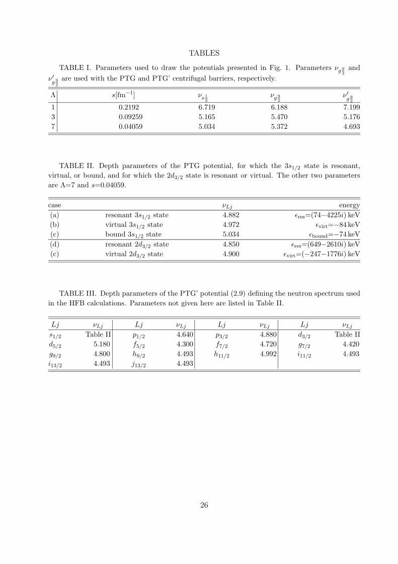
TABLE I. Parameters used to draw the potentials presented in Fig. 1. Parameters νg 92

andν ′

g 92

are used with the PTG and PTG’ centrifugal barriers, respectively.

Λ s[fm−1] νs 12

νg 92

ν ′g 9

2

1 0.2192 6.719 6.188 7.1993 0.09259 5.165 5.470 5.1767 0.04059 5.034 5.372 4.693

TABLE II. Depth parameters of the PTG potential, for which the 3s1/2 state is resonant,virtual, or bound, and for which the 2d3/2 state is resonant or virtual. The other two parametersare Λ=7 and s=0.04059.

case νLj energy(a) resonant 3s1/2 state 4.882 εres=(74−4225i) keV(b) virtual 3s1/2 state 4.972 εvirt=−84 keV(c) bound 3s1/2 state 5.034 εbound=−74 keV(d) resonant 2d3/2 state 4.850 εres=(649−2610i) keV(c) virtual 2d3/2 state 4.900 εvirt=(−247−1776i) keV

TABLE III. Depth parameters of the PTG’ potential (2.9) defining the neutron spectrum usedin the HFB calculations. Parameters not given here are listed in Table II.

Lj νLj Lj νLj Lj νLj Lj νLj

s1/2 Table II p1/2 4.640 p3/2 4.880 d3/2 Table IId5/2 5.180 f5/2 4.300 f7/2 4.720 g7/2 4.420g9/2 4.800 h9/2 4.493 h11/2 4.992 i11/2 4.493i13/2 4.493 j13/2 4.493

26

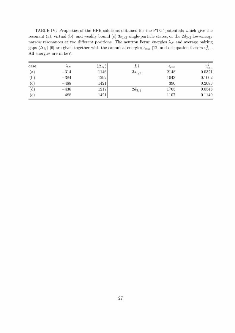
TABLE IV. Properties of the HFB solutions obtained for the PTG’ potentials which give theresonant (a), virtual (b), and weakly bound (c) 3s1/2 single-particle states, or the 2d3/2 low-energynarrow resonances at two different positions. The neutron Fermi energies λN and average pairinggaps 〈∆N 〉 [6] are given together with the canonical energies εcan [12] and occupation factors v2

can.All energies are in keV.

case λN 〈∆N 〉 Lj εcan v2can

(a) −314 1146 3s1/2 2148 0.0321(b) −384 1292 1043 0.1002(c) −488 1421 390 0.2083(d) −436 1217 2d3/2 1765 0.0548(c) −488 1421 1107 0.1149

27

FIGURES

- 6 0

- 4 0

- 2 0

0

0 5 1 0 1 5r ( f m )

L = 0

- 2 0

0

2 0

VP

TG (

Me

V) L = 4

- 2 0

0

2 0 L = 4

w i t h L ( L + 1 ) / r 2

ΛΛ == 11

ΛΛ == 33

ΛΛ == 77

FIG. 1. Radial PTG potentials for three values of the parameter Λ (see Table VII for thecomplete set of parameters). The bottom panel shows the potential for L=0, while the middleand top panels correspond to L=4 and the PTG (2.1) and PTG’ (2.9) potentials, respectively (seetext).

28

Momentum plane

Energy plane (physical sheet)

Energy plane (unphysical sheet)

Virtual states

Bound states

’Crazy’ resonances

κAnti-resonances Resonances

ℑ

ℑ

ℑ

ℜ

ℜ

ℜ

(k)

(k)

(ε)

(ε)

(ε)

(ε)

Bound states

Anti-resonances

Resonances

’Crazy’ resonances

Virtual states

κ

(a)

(b)

(c)

FIG. 2. Schematic representation of different domains of S-matrix poles in the complex mo-mentum and energy planes.

29

0

1

2

3

4

0 10 20 30r (fm )

3s 1/2

Wa

ve

fu

nc

tio

n (

fm-1

/2)

-0.2

0

0.2

0 2 4 6

FIG. 3. Radial PTG wave functions of the 3s1/2 state calculated analytically for parameterslisted in Table II. The dotted, dashed, and solid lines correspond to resonant, virtual, and bound3s1/2 states, respectively. In the inset the same wave functions are shown in the region of attractivepotential. Volume element 4πr2 is included in the definition of wave functions.

30

-2

0

2

0 20 40 60Energy (M eV)

Ph

as

e s

hif

t (r

ad

) s 1/2

39-18 i M eV

(b)

0.10

0.20

0.30

Lo

ca

liza

tio

n

39-18 i M eV

(a)

FIG. 4. Localization [Eq. (4.19)] (a) and phase shift (b) of the s1/2 continuum PTG states.Circles denote results of numerical calculations performed in the box of 30 fm. Solid and dashedlines show the localizations calculated analytically for scattering wave functions normalized in thebox of 30 fm, and to a constant amplitude of the outgoing wave, respectively. Arrows indicateposition of the lowest, very broad, resonance. Parameters of the PTG potential are given inTable II (bound 3s1/2 state).

31

0.00

0.10

0.20

0.30εε res =(74-4225i) keV(a)

0.00

0.10

0.20

0.30

H FB

PTG

Lo

ca

liza

tio

n

s 1 /2

εε v irt =-84 keV(b )

0.00

0.10

0.20

0.30

0 5 10 15 20

Energy (M eV)

εε bound =-74 keV(c)

FIG. 5. Localization [Eq. (4.19)] of the HFB upper components (dots) of the quasiparticlestates, compared with the localization of the s1/2 continuum PTG states (lines).

32

-2

-1

0

1

2

3εε res =(74-4225i) keV(a)

-2

-1

0

1

2

3

H FB

PTG

Ph

as

e s

hif

t (r

ad

)

s 1 /2

εε v irt =-84 keV(b )

-2

-1

0

1

2

3

0 5 10 15 20

Energy (M eV)

εε bound =-74 keV(c)

FIG. 6. Phase shifts of the HFB upper components (dots) of the quasiparticle states, comparedwith the phase shifts of the s1/2 continuum PTG states (lines).

33

-0.2

-0.1

0

0.1

0.2

0 5 10 15 20

(a)

(b)

(c)

3s 1/2

Ca

no

nic

al

w.f

. (f

m-1

/2)

r (fm )

0.01

0.1

0 10 20

FIG. 7. Canonical wave functions of the 3s1/2 state, corresponding to the three cases of theHFB calculations listed in Table IV. The dotted, dashed, and solid lines correspond to resonant,virtual, and bound PTG 3s1/2 states, respectively. In the inset the same wave functions are shownin the logarithmic scale. Volume element 4πr2 is included in the definition of wave functions.

34

0.00

0.02

0.04

0.06

0.08

0 5 10 15 20

Nn

Energy (M eV)

10-4

10-3

10-2

10-1

0 5 10 15

(a)(b)(c)

s 1/2

FIG. 8. Norms Nn of the s1/2 lower quasiparticle wave functions φ2(En, rσ), corresponding tothe three cases of the HFB calculations listed in Table IV. Inset shows the same values in thelogarithmic scale.

35

0.0

0.2

0.4

0.6

0.8PTG '

HFB

0 10 20 30 40

(41-18i) M eV(c)

Energy (M eV)

0.2

0.4

0.6

0.8

1.0

(42-18 i) M eV(d)

d 3/2

0.0

0.4

0.8

0 2 4

0.0

0.4

0.8

0 2 4

Lo

ca

liza

tio

n

FIG. 9. Localization of the HFB upper components (dots) of the quasiparticle states comparedwith the localization of the d3/2 continuum PTG’ states (lines). Upper (a) and lower (b) panelsdiffer by the position of the 2d3/2 resonances with respect to the top of the centrifugal barrier, seetext.

36

0.00

0.02

0.04

0.06

0.08

0 5 10 15 20

Nn

Energy (M eV)

10-4

10-3

10-2

10-1

0 5 10 15

(d)

(c)

d 3/2

FIG. 10. Norms Nn of the d3/2 lower quasiparticle wave functions φ2(En, rσ), correspondingto the two cases of the HFB calculations listed in Table IV. Inset shows the same values in thelogarithmic scale.

37

0.0

0.3

0.6

HFB

PTG '

d 3/2

0.0

0.3

0.6

0.0

0.3

0.6

Lo

ca

liza

tio

n

0 .0

0.3

0.6

0.0

0.3

0.6

0.0

0.3

0.6

0 5 10 15

Energy (M eV)

FIG. 11. Localizations of the HFB upper components of the d3/2 quasiparticle states (dots)compared with those of the d3/2 continuum PTG’ states (lines). The six panels differ by thepositions of the lowest d3/2 resonance with respect to the top of the centrifugal barrier, see text.Arrows indicate values of the canonical energies εcan of the 2d3/2 canonical states.

38

0.0000

0.0005

HFB

d 3/2v can =0.0015

0.0000

0.0005v can =0.0023

0.000

0.001

Nn

v can =0.004

0.000

0.003 v can =0.009

0.00

0.01v can =0.027

0.00

0.05

0 5 10 15

Energy (M eV)

v can =0.11

FIG. 12. Norms Nn of the HFB lower components φ2(En, rσ) of the d3/2 quasiparticle states.In each panel (similarly as in Fig. 11), arrows indicate values of the canonical energies εcan of the2d3/2 canonical states, while the corresponding occupation factors vcan are given explicitly.

39