continuoustimestructuralequationmodeling with r package ctsem
TRANSCRIPT

JSS Journal of Statistical SoftwareApril 2017, Volume 77, Issue 5. doi: 10.18637/jss.v077.i05
Continuous Time Structural Equation Modelingwith R Package ctsem
Charles C. DriverMax Planck Institute
for Human Development
Johan H. L. OudRadboud University
Nijmegen
Manuel C. VoelkleHumboldt University Berlin
Max Planck Institutefor Human Development
Abstract
We introduce ctsem, an R package for continuous time structural equation modelingof panel (N > 1) and time series (N = 1) data, using full information maximum likelihood.Most dynamic models (e.g., cross-lagged panel models) in the social and behaviouralsciences are discrete time models. An assumption of discrete time models is that timeintervals between measurements are equal, and that all subjects were assessed at the sameintervals. Violations of this assumption are often ignored due to the difficulty of account-ing for varying time intervals, therefore parameter estimates can be biased and the timecourse of effects becomes ambiguous. By using stochastic differential equations to estimatean underlying continuous process, continuous time models allow for any pattern of mea-surement occasions. By interfacing to OpenMx, ctsem combines the flexible specificationof structural equation models with the enhanced data gathering opportunities and im-proved estimation of continuous time models. ctsem can estimate relationships over timefor multiple latent processes, measured by multiple noisy indicators with varying timeintervals between observations. Within and between effects are estimated simultaneouslyby modeling both observed covariates and unobserved heterogeneity. Exogenous shockswith different shapes, group differences, higher order diffusion effects and oscillating pro-cesses can all be simply modeled. We first introduce and define continuous time models,then show how to specify and estimate a range of continuous time models using ctsem.
Keywords: time series, longitudinal modeling, panel data, state space, structural equationmodeling, continuous time, stochastic differential equation, dynamic models, Kalman filter, R.
1. IntroductionDynamic models, such as the well known vector autoregressive model, are widely used inthe social and behavioral sciences. They allow us to see how fluctuations in processes re-

2 ctsem: Continuous Time Structural Equation Modeling in R
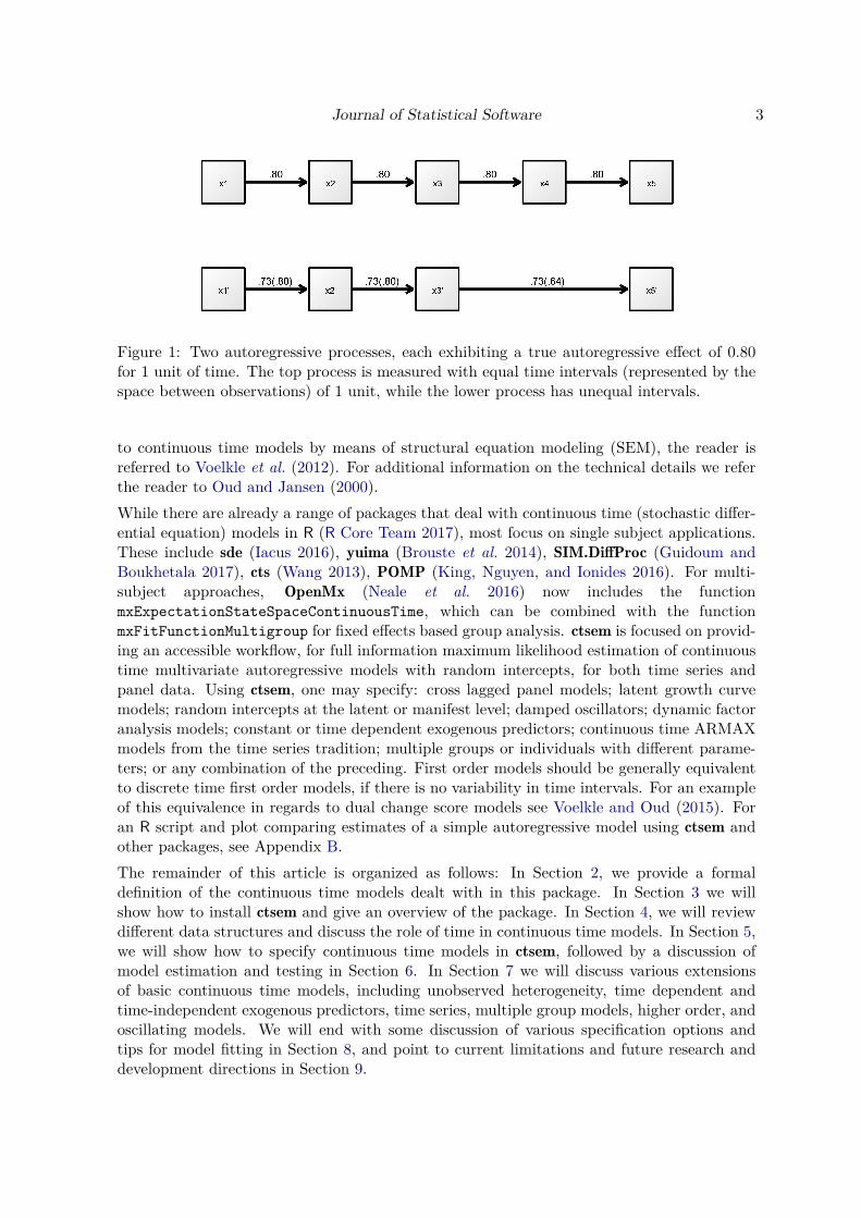
late to later values of those processes, the effect of an input at a particular time, how thevarious factors relate to average levels of the processes, and many other possibilities. Someexamples with panel data include the impact of European institutional changes on businesscycles (Canova, Ciccarelli, and Ortega 2012), the coupling between sensory and intellectualfunctioning (Ghisletta and Lindenberger 2005), or the analysis of bidirectional links betweenchildren’s delinquency and the quality of parent-child relationships (Keijsers, Loeber, Branje,and Meeus 2011). Examples of single subject approaches are studies on the decline in pneu-monia rates in the USA after a vaccine introduction (Grijalva, Nuorti, Arbogast, Martin,Edwards, and Griffin 2007), or the lack of a relationship between antidepressant sales andpublic health in Iceland (Helgason, Tomasson, and Zoega 2004). At present, applications ofdynamic models in the social and behavioral sciences are almost exclusively limited to discretetime models. In discrete time models it is generally assumed that time progresses in discretesteps, that time intervals between measurement occasions are equal, and that, in case of paneldata, subjects are assessed with the same time intervals. In many cases, these assumptionsare not met, resulting in biased parameter estimates and a misunderstanding of the strengthand time course of effects. This concept is illustrated in Figure 1 (with a comprehensiveexample in Appendix A). In the upper panel, Figure 1 shows a true autoregressive effect of0.80 between observed variables (represented by squares), assuming equal intervals of length∆t = 1 (represented by equal distances between observed variables), while the lower panelshows a process with two intervals of ∆t = 1 and one interval ∆t = 2. In the top panel, themeaning of the estimate of 0.80 is clear – it refers to the autoregression estimate for 1 unit oftime. In the lower case, however, the autoregression estimate of 0.73 is ambiguous – it is toolow to characterize the relation between the first three occasions (correct value of 0.80 is inbrackets) and too high between the last two occasions (correct value of 0.64).
Obviously, parameter estimates and, thus, scientific conclusions, are biased when observationintervals vary and this is not adequately accounted for. In simple cases, such as the examplein Figure 1, additional variables – so called phantom variables (Rindskopf 1984), with missingvalues for all individuals – could be added in order to artificially create equally spaced timeintervals. For example, an additional variable could be specified at t4, resulting in equal timeintervals and permitting the use of standard discrete time models. For complex patternsof individually varying time intervals, however, this approach quickly becomes untenable(Voelkle and Oud 2013). Furthermore, with discrete time models it is difficult to compareresults obtained from different studies with unequal time intervals, which poses a limitationto the production of cumulative knowledge in science (Voelkle, Oud, Davidov, and Schmidt2012).
Continuous time models overcome these problems, offering researchers the possibility to es-timate parameters free from bias due to unequal intervals, easily compare between studiesand data sets with different observation schedules, gather data with variable time intervalsbetween observations, understand changes in observed effects over time, and parsimoniouslyspecify complex dynamics. Although continuous time models have a long history (Coleman1964; Hannan and Tuma 1979), their use in the social sciences is still uncommon. At leastin part, this is due to a lack of suitable software to specify and estimate continuous timemodels. With the introduction of ctsem (Driver, Voelkle, and Oud 2017) in this article, wewant to overcome this limitation. Although we will define continuous time models in the nextsection and provide several examples in the sections thereafter, a comprehensive treatment ofcontinuous time models is beyond the scope of this article. For a more general introduction
Journal of Statistical Software 3
Figure 1: Two autoregressive processes, each exhibiting a true autoregressive effect of 0.80for 1 unit of time. The top process is measured with equal time intervals (represented by thespace between observations) of 1 unit, while the lower process has unequal intervals.
to continuous time models by means of structural equation modeling (SEM), the reader isreferred to Voelkle et al. (2012). For additional information on the technical details we referthe reader to Oud and Jansen (2000).While there are already a range of packages that deal with continuous time (stochastic differ-ential equation) models in R (R Core Team 2017), most focus on single subject applications.These include sde (Iacus 2016), yuima (Brouste et al. 2014), SIM.DiffProc (Guidoum andBoukhetala 2017), cts (Wang 2013), POMP (King, Nguyen, and Ionides 2016). For multi-subject approaches, OpenMx (Neale et al. 2016) now includes the functionmxExpectationStateSpaceContinuousTime, which can be combined with the functionmxFitFunctionMultigroup for fixed effects based group analysis. ctsem is focused on provid-ing an accessible workflow, for full information maximum likelihood estimation of continuoustime multivariate autoregressive models with random intercepts, for both time series andpanel data. Using ctsem, one may specify: cross lagged panel models; latent growth curvemodels; random intercepts at the latent or manifest level; damped oscillators; dynamic factoranalysis models; constant or time dependent exogenous predictors; continuous time ARMAXmodels from the time series tradition; multiple groups or individuals with different parame-ters; or any combination of the preceding. First order models should be generally equivalentto discrete time first order models, if there is no variability in time intervals. For an exampleof this equivalence in regards to dual change score models see Voelkle and Oud (2015). Foran R script and plot comparing estimates of a simple autoregressive model using ctsem andother packages, see Appendix B.The remainder of this article is organized as follows: In Section 2, we provide a formaldefinition of the continuous time models dealt with in this package. In Section 3 we willshow how to install ctsem and give an overview of the package. In Section 4, we will reviewdifferent data structures and discuss the role of time in continuous time models. In Section 5,we will show how to specify continuous time models in ctsem, followed by a discussion ofmodel estimation and testing in Section 6. In Section 7 we will discuss various extensionsof basic continuous time models, including unobserved heterogeneity, time dependent andtime-independent exogenous predictors, time series, multiple group models, higher order, andoscillating models. We will end with some discussion of various specification options andtips for model fitting in Section 8, and point to current limitations and future research anddevelopment directions in Section 9.

4 ctsem: Continuous Time Structural Equation Modeling in R
2. Continuous time models: Fundamentals
The class of continuous time models implemented in ctsem is represented by the multivariatestochastic differential equation:
dηi(t) =(Aηi(t) + ξi + Bzi +Mχi(t)
)dt +GdWi(t). (1)
Vector ηi(t) ∈ Rv is a v-variable vector of the processes of interest at time t, for subject i. Thematrix A ∈ Rv×v represents the so-called drift matrix, with auto effects on the diagonal andcross effects on the off-diagonals characterizing the temporal relationships of the processes.The long term level of processes ηi(t) is determined by the v-length vector of random variablesξi, with ξi ∼ N(κ,φξ) for every i, where vector κ ∈ Rv denotes the continuous time intercepts,and matrix φξ ∈ Rv×v the covariance across subjects. ξi sets the long-term level of theprocesses and the long-term differences between the processes of individual subjects – withoutit the processes of a stable model would all trend towards zero in the long-run.The matrix B ∈ Rv×p represents the effect of the p-length vector of (fixed) time-independentpredictors z ∈ Rp on processes ηi(t). Time-independent predictors would typically be variablesthat differ between subjects, but are constant within subjects for the time range in question.Time-dependent predictors χi(t) represent inputs to the system that vary over time and areindependent of fluctuations in the system. Equation 1 shows a generalized form for time-dependent predictors, that could be treated in a variety of ways dependent on the assumedtime course (or shape) of time-dependent predictors. We use a simple impulse form, in whichthe predictors are treated as impacting the processes only at the instant of an observation.When necessary, the evolution over time can be modeled by extending the state matrices.This is demonstrated in the level change example in Section 7.1, wherein a model containingonly the basic impulse has a persistent level change effect added. To achieve the impulse formwe replace part of Equation 1 as follows:
χi(t) =∑u∈Ui
xi,uδ(t − u). (2)
Here, time-dependent predictors xi,u ∈ Rl are observed at times u ∈ Ui ⊂ R. The Dirac deltafunction δ(t − u) is a generalized function that is ∞ at 0 and 0 elsewhere, yet has an integralof 1 (when 0 is in the range of integration). It is useful to model an impulse to a system, andhere is scaled by the vector of time-dependent predictors xi,u. The effect of these impulses onprocesses ηi(t) is then M ∈ Rv×l.Wi(t) ∈ Rv represent independent Wiener processes, with a Wiener process being a random-walk in continuous time. dWi(t) is meaningful in the context of stochastic differential equa-tions, and represents the stochastic error term, an infinitesimally small increment of theWiener process. The lower triangular matrix G ∈ Rv×v represents the effect of this noise onthe change in ηi(t). Q, where Q = GG>, represents the variance-covariance matrix of thediffusion process in continuous time.The solution of the stochastic differential Equation 1 for any time interval t − t0, with t > t0

Journal of Statistical Software 5
is:
ηi(t) = eA(t−t0)ηi(t0) +A−1[eA(t−t0) − I]ξi +A−1[eA(t−t0) − I]Bzi +
M∑u∈Ui
xi,uδ(t − u) +∫ t
t0
eA(t−s)GdWi(s) (3)
The five summands of this equation correspond to the five of Equation 1, and give the linkbetween the continuous time model and discrete instantiations of the process.The last summand of Equation 3, the integral of the diffusion over the given time interval,exhibits the covariance matrix:
cov[ ∫ t
t0
eA(t−s)GdWi(s)]=
∫ t
t0
eA(t−s)QeA>(t−s)ds = irow(A−1
# [eA#(t−t0) − I] row(Q)
), (4)
where A# = A ⊗ I + I ⊗A, with ⊗ denoting the Kronecker-product, row is an operation thattakes elements of a matrix rowwise and puts them in a column vector, and irow is the inverseof the row operation.The process vector ηi(t) may be directly observed or latent with measurement model
yi(t) = Γi + Ληi(t) + ζi(t), where ζ(t) ∼ N(0,Θ), and Γ ∼ N(τ,Ψ), (5)
where c-length vector τ is the expected value of Γi, which is distributed across subjectsaccording to covariance matrix Ψ ∈ Rc×c (referred to later as manifest traits – see Section 7.1).Λ ∈ Rc×v is a matrix of factor loadings, yi(t) ∈ Rc is a vector of manifest variables, and residualvector ζi ∈ Rc has covariance matrix Θ ∈ Rc×c.
2.1. Continuous time and SEM
Continuous time models have already been implemented as structural equation models, usingeither non-linear algebraic constraints (Oud and Jansen 2000) or linear approximations of thematrix exponential (Oud 2002). Our formulation uses either the SEM RAM (reticular actionmodel) specification as per McArdle and McDonald (1984), or the state space form recentlyadded to OpenMx (Neale et al. 2016; Hunter 2014). For details on the equivalence and differ-ences between SEM and state space modeling techniques, see Chow, Ho, Hamaker, and Dolan(2010). ctsem translates user specified input matrices and switches into an OpenMx modelconsisting of continuous time parameter matrices, algebraic transformations of these matri-ces to aid optimization (see Section 6), and algebraic transforms from the continuous timeparameters to discrete time parameters for every unique time interval. Expectation matricesare then generated for each individual according to the specified inputs, constraints, and ob-served timing data. Optimization using either the Kalman filter or rowwise full informationmaximum likelihood (FIML) within OpenMx is used to estimate the parameters, typicallywith a first pass using a penalty term (or prior) to find a region of high probability withoutextreme parameters, and then a second FIML pass using the first as starting value.
6 ctsem: Continuous Time Structural Equation Modeling in R
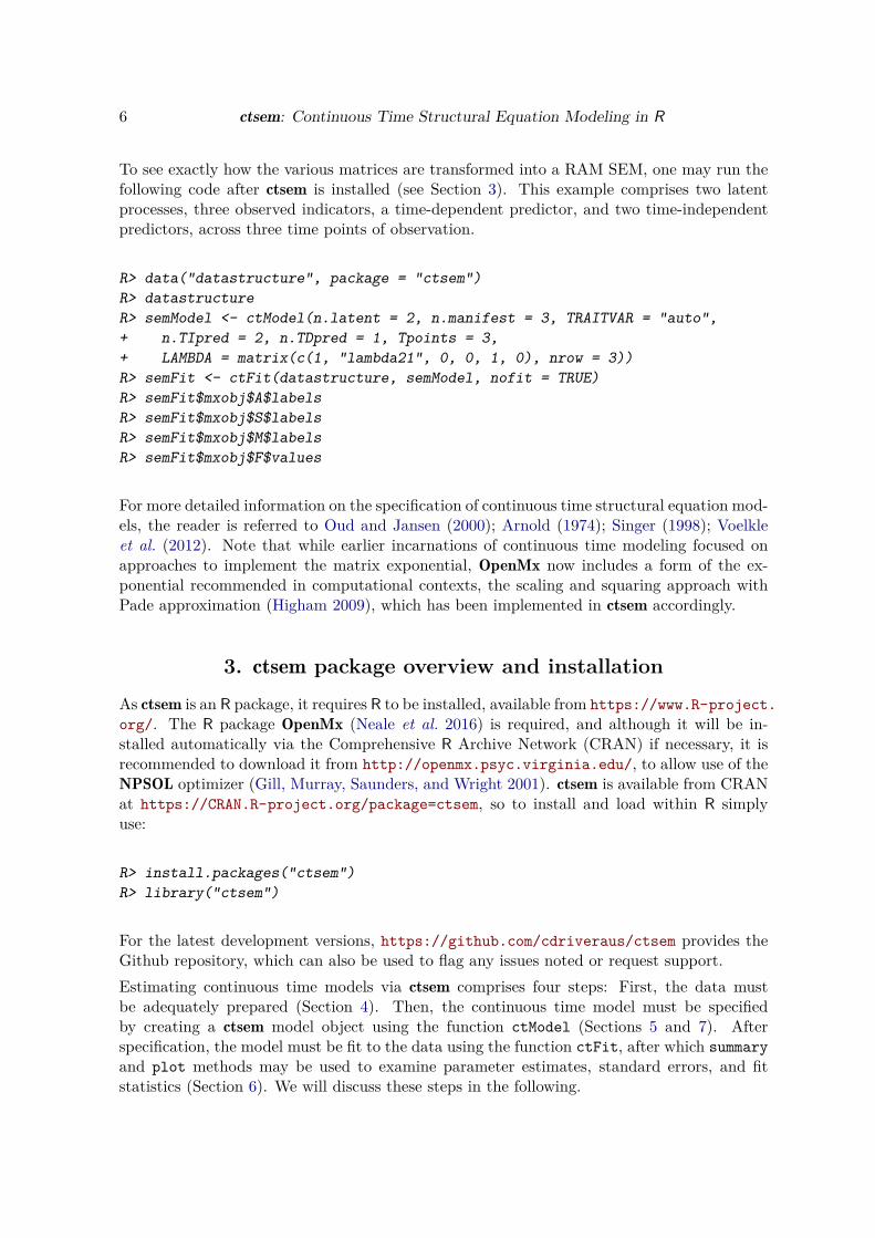
To see exactly how the various matrices are transformed into a RAM SEM, one may run thefollowing code after ctsem is installed (see Section 3). This example comprises two latentprocesses, three observed indicators, a time-dependent predictor, and two time-independentpredictors, across three time points of observation.
R> data("datastructure", package = "ctsem")R> datastructureR> semModel <- ctModel(n.latent = 2, n.manifest = 3, TRAITVAR = "auto",+ n.TIpred = 2, n.TDpred = 1, Tpoints = 3,+ LAMBDA = matrix(c(1, "lambda21", 0, 0, 1, 0), nrow = 3))R> semFit <- ctFit(datastructure, semModel, nofit = TRUE)R> semFit$mxobj$A$labelsR> semFit$mxobj$S$labelsR> semFit$mxobj$M$labelsR> semFit$mxobj$F$values
For more detailed information on the specification of continuous time structural equation mod-els, the reader is referred to Oud and Jansen (2000); Arnold (1974); Singer (1998); Voelkleet al. (2012). Note that while earlier incarnations of continuous time modeling focused onapproaches to implement the matrix exponential, OpenMx now includes a form of the ex-ponential recommended in computational contexts, the scaling and squaring approach withPade approximation (Higham 2009), which has been implemented in ctsem accordingly.
3. ctsem package overview and installation
As ctsem is an R package, it requires R to be installed, available from https://www.R-project.org/. The R package OpenMx (Neale et al. 2016) is required, and although it will be in-stalled automatically via the Comprehensive R Archive Network (CRAN) if necessary, it isrecommended to download it from http://openmx.psyc.virginia.edu/, to allow use of theNPSOL optimizer (Gill, Murray, Saunders, and Wright 2001). ctsem is available from CRANat https://CRAN.R-project.org/package=ctsem, so to install and load within R simplyuse:
R> install.packages("ctsem")R> library("ctsem")
For the latest development versions, https://github.com/cdriveraus/ctsem provides theGithub repository, which can also be used to flag any issues noted or request support.Estimating continuous time models via ctsem comprises four steps: First, the data mustbe adequately prepared (Section 4). Then, the continuous time model must be specifiedby creating a ctsem model object using the function ctModel (Sections 5 and 7). Afterspecification, the model must be fit to the data using the function ctFit, after which summaryand plot methods may be used to examine parameter estimates, standard errors, and fitstatistics (Section 6). We will discuss these steps in the following.

Journal of Statistical Software 7
4. Data structureThe internal functions of ctFit use data in a wide layout, with all data for each individual ina single row, including the time intervals between measurement occasions for this individual.Because this is the format used internally when fitting, for the sake of transparency it isalso required as the input format, and is detailed below in Section 4.1. In some cases itmay however be simpler to maintain data in a long format, and use the ctLongToWide andctIntervalise functions we provide to convert from long format with absolute times to wideformat with time intervals. This functionality is discussed in Section 4.2. The choice of timescale and treatment of the initial time point can influence results and will be discussed inSection 4.3, though first time users may find it easier to return to it later.
4.1. Wide format
This is the data format required when fitting a model with ctsem. The example data belowdepicts two individuals, observed at three occasions, on three manifest variables, one time-dependent predictor, and two time-independent predictors. A corresponding path diagram ofone possible model for this data is shown in Figure 2. The data are ordered into blocks as fol-lows: manifest process variables, time-dependent predictors, time intervals, time-independentpredictors. Manifest variables are grouped by measurement occasion and ordered within thisby variable. In the example there are three manifest variables (Y1, Y2, Y3) assessed acrossthree measurement occasions. In this case, the first three columns of the data (Y1_T0, Y2_T0,Y3_T0) represent the three manifest variables at the first measurement occasion, time point 0,followed by the columns of the second measurement occasion and so on. Note that measure-ment occasions subsequent to the first may occur at different times for different individuals.Also note the naming convention, wherein the variable name is followed by an underscoreand T, followed by an integer denoting the measurement occasion, beginning at T0. After themanifest variables, any time-dependent predictors (there need not be any) are also groupedby measurement occasion and ordered within this by variable (changed since v2.2.0). Theseare named in the same way as the manifest variables, with the predictor name preceded byan underscore and T, then the measurement occasion integer beginning from 0. In the databelow and the model in Figure 2, there is only one time dependent predictor, TD1, thoughmore could be added. After the time-dependent predictors, T − 1 time intervals are specifiedin chronological order, with column names dT followed by the number of the measurementoccasion occurring after the interval . That is, dT1 refers to the time interval between the firstmeasurement occasion, T0, and the second, T1. In continuous time modelling it is imperativeto know the time point at which an observation takes place. Thus, while missing values onobserved scores are no problem, missing values on time intervals are not allowed. Finally, twotime-independent predictors (TI1, TI2 – the naming here is only with variable names) arecontained in the last two columns of the data structure.
Y1_T0 Y2_T0 Y3_T0 Y1_T1 Y2_T1 Y3_T1 Y1_T2 Y2_T2 Y3_T2 TD1_T0 TD1_T1 TD1_T21 0.44 -0.83 -0.17 1.13 -2.44 0.31 NA NA NA -1.67 0.15 NA2 NA 6.84 9.22 8.24 9.04 7.88 6.45 8.39 7.16 0.81 -1.97 -1.6
dT1 dT2 TI1 TI21 0.65 0.001 0.06 -2.052 2.56 2.260 2.22 -1.41

8 ctsem: Continuous Time Structural Equation Modeling in R
Figure 2: The first three time points of a two process continuous time model, with threemanifest indicators (blue) measuring 2 latent processes (purple), one time-dependent predictor(dark green), and two time-independent predictors (light green). Variance/covariance pathsare in orange, regressions in red. Light gray paths indicate those that are constrained to afunction of other parameters. Note that the value of parameters for all paths to latents attime 2 and higher do not directly represent the effect, rather, the effect depends on a functionincluding the shown parameter and the time interval ∆t. Manifest intercepts are not shownhere.
4.2. Conversion from long format with absolute times
Although ctsem uses the wide format as default data input, often data are stored in longformat, that is, each subject has multiple rows of data, with each row reflecting a particu-lar measurement occasion. In addition, time intervals may not be readily available at theindividual level, instead the absolute time when a measurement took place is recorded. Toconvert from long format, the data must contain a subject identification column, columns forevery observed variable, and a time variable. Unlike for the wide format data, at this pointadditional unused variables in the long structure are no problem. In the example below, threemanifest variables of interest (Y1, Y2, Y3) have been observed across a number of occasions,
Journal of Statistical Software 9
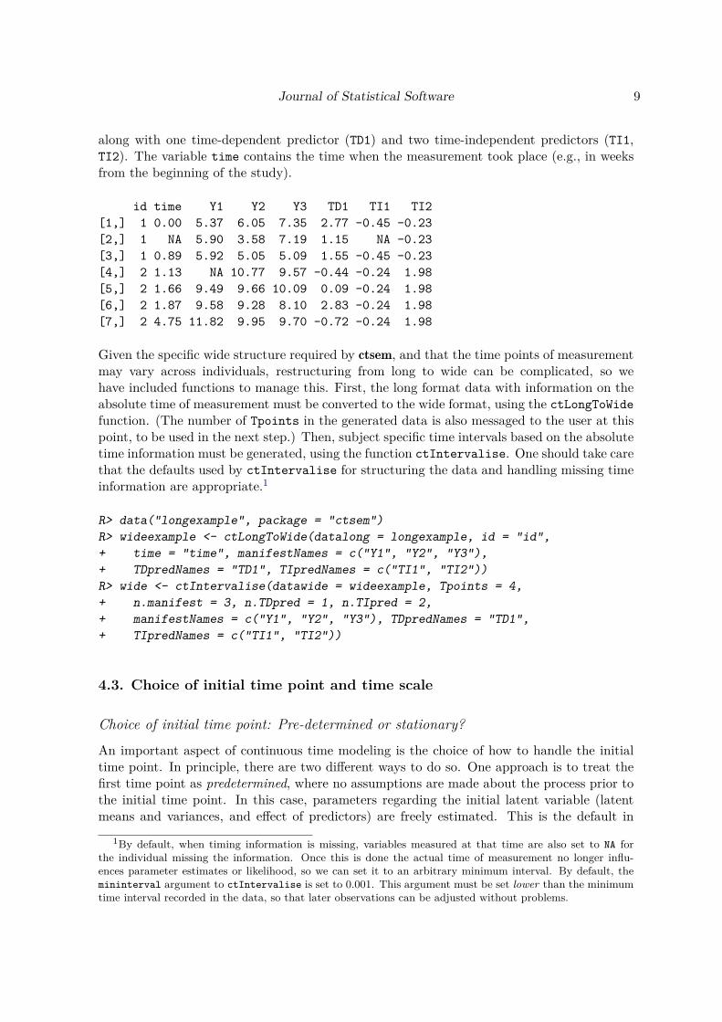
along with one time-dependent predictor (TD1) and two time-independent predictors (TI1,TI2). The variable time contains the time when the measurement took place (e.g., in weeksfrom the beginning of the study).
id time Y1 Y2 Y3 TD1 TI1 TI2[1,] 1 0.00 5.37 6.05 7.35 2.77 -0.45 -0.23[2,] 1 NA 5.90 3.58 7.19 1.15 NA -0.23[3,] 1 0.89 5.92 5.05 5.09 1.55 -0.45 -0.23[4,] 2 1.13 NA 10.77 9.57 -0.44 -0.24 1.98[5,] 2 1.66 9.49 9.66 10.09 0.09 -0.24 1.98[6,] 2 1.87 9.58 9.28 8.10 2.83 -0.24 1.98[7,] 2 4.75 11.82 9.95 9.70 -0.72 -0.24 1.98
Given the specific wide structure required by ctsem, and that the time points of measurementmay vary across individuals, restructuring from long to wide can be complicated, so wehave included functions to manage this. First, the long format data with information on theabsolute time of measurement must be converted to the wide format, using the ctLongToWidefunction. (The number of Tpoints in the generated data is also messaged to the user at thispoint, to be used in the next step.) Then, subject specific time intervals based on the absolutetime information must be generated, using the function ctIntervalise. One should take carethat the defaults used by ctIntervalise for structuring the data and handling missing timeinformation are appropriate.1
R> data("longexample", package = "ctsem")R> wideexample <- ctLongToWide(datalong = longexample, id = "id",+ time = "time", manifestNames = c("Y1", "Y2", "Y3"),+ TDpredNames = "TD1", TIpredNames = c("TI1", "TI2"))R> wide <- ctIntervalise(datawide = wideexample, Tpoints = 4,+ n.manifest = 3, n.TDpred = 1, n.TIpred = 2,+ manifestNames = c("Y1", "Y2", "Y3"), TDpredNames = "TD1",+ TIpredNames = c("TI1", "TI2"))
4.3. Choice of initial time point and time scale
Choice of initial time point: Pre-determined or stationary?
An important aspect of continuous time modeling is the choice of how to handle the initialtime point. In principle, there are two different ways to do so. One approach is to treat thefirst time point as predetermined, where no assumptions are made about the process prior tothe initial time point. In this case, parameters regarding the initial latent variable (latentmeans and variances, and effect of predictors) are freely estimated. This is the default in
1By default, when timing information is missing, variables measured at that time are also set to NA forthe individual missing the information. Once this is done the actual time of measurement no longer influ-ences parameter estimates or likelihood, so we can set it to an arbitrary minimum interval. By default, themininterval argument to ctIntervalise is set to 0.001. This argument must be set lower than the minimumtime interval recorded in the data, so that later observations can be adjusted without problems.

10 ctsem: Continuous Time Structural Equation Modeling in R
ctsem, though it requires some constraining if fitting a single individual.2 When treating thefirst time point as predetermined, it is important to choose a meaningful starting point, asthe process will gradually transition from the variances and means of the initial parameters,towards those of the parameters when the model is stationary. In principle, the initial timepoint does not have to reflect the first measurement occasion, and can also be set to any timeprior. For example it may be of interest to set T0 to the beginning of the school year, althoughthe first measurement was only taken two weeks after start of school. This can be specifiedusing the startoffset argument to ctIntervalise, specifying the amount of time priorto the first observed measurement occasion. The other approach is to assume a stationarymodel, that is, a model where the first observations are merely random instantiations of a longterm process with time-invariant mean and variance expectations. Or, put another way, weassume that sufficient time has elapsed from the unobserved, hypothetical start of the processto our first measurement occasion, such that whatever the start values were, they no longerinfluence the process. Strictly speaking, this requires an infinite length of time, or a processthat began in a stationary state. However, in some practical cases without clear trends inthe data it is possible that the improvement in estimation due to the stationarity assumptionoutweighs related losses (this may also be tested). To implement the stationarity assumptionthe means and variances of the first measurement occasion are constrained according to themodel predicted means and variances across all time points. This is specified by includinga character vector of the T0 matrices to constrain in the ctFit arguments: stationary =c("T0VAR", "T0MEANS") constrains both means and variances to stationarity. The ctModelspecification of any matrices that are constrained to stationarity is ignored. Note that anybetween-subject variance parameters, factor loadings, manifest residuals, as well as drift anddiffusion parameters, are inherently stationary (given the configuration of ctsem). Morecomplex model specification within ctsem, or direct modification of the generated OpenMxmodel, is necessary for modeling time variability in the parameters.
Choice of time scale: Individual or sample relative time?
An additional consideration when treating the first time point as predetermined is necessaryin cases of individually varying time intervals. Here, two alternatives need to be distinguished.The default option is to treat the observation times as relative to the individual, the other isto treat them as relative to the sample. When we treat time as relative to the individual, thefirst observation of every individual is set to measurement occasion T0, even though differentindividuals may have been recorded many years apart. However if we treat time as relative tothe sample, every individual’s observation times are set relative to the very first observation inthe entire sample. This may result in a larger and sparser data matrix, potentially with onlya single observation at the first measurement occasion. To specify sample relative time whenconverting from absolute time to intervals, set the argument individualRelativeTime =FALSE in the ctIntervalise function. The choice between the individual or sample relativetime may influence parameter estimates when the processes are not stationary. One way ofdeciding between the two may be to observe whether the changes of the individuals’ processesis more closely aligned with the sample relative or individual relative time. The changein processes may be more aligned with individual relative time when we expect that theactivity of measurement relates to changes in the process. Consider for instance the relationbetween abstinence behavior and mood among individuals attending an alcohol addiction
2Either "T0VAR" or "T0MEANS" must be fixed, see Section 7.3.
Journal of Statistical Software 11
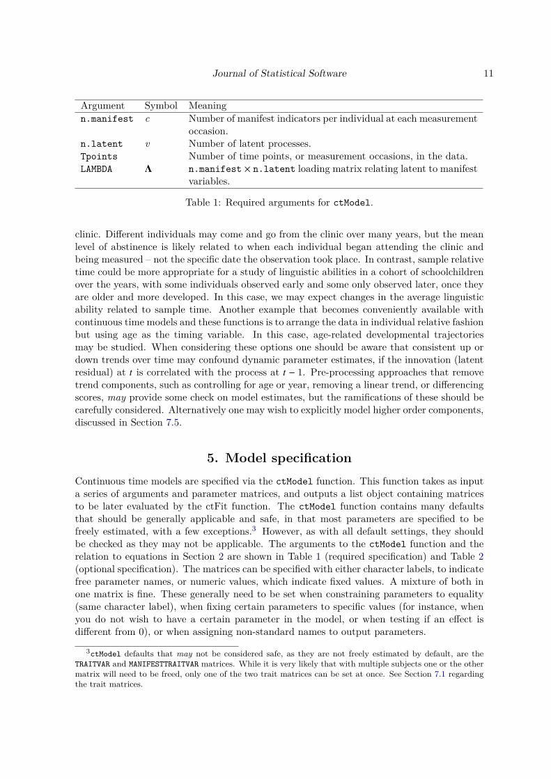
Argument Symbol Meaningn.manifest c Number of manifest indicators per individual at each measurement
occasion.n.latent v Number of latent processes.Tpoints Number of time points, or measurement occasions, in the data.LAMBDA Λ n.manifest × n.latent loading matrix relating latent to manifest
variables.
Table 1: Required arguments for ctModel.
clinic. Different individuals may come and go from the clinic over many years, but the meanlevel of abstinence is likely related to when each individual began attending the clinic andbeing measured – not the specific date the observation took place. In contrast, sample relativetime could be more appropriate for a study of linguistic abilities in a cohort of schoolchildrenover the years, with some individuals observed early and some only observed later, once theyare older and more developed. In this case, we may expect changes in the average linguisticability related to sample time. Another example that becomes conveniently available withcontinuous time models and these functions is to arrange the data in individual relative fashionbut using age as the timing variable. In this case, age-related developmental trajectoriesmay be studied. When considering these options one should be aware that consistent up ordown trends over time may confound dynamic parameter estimates, if the innovation (latentresidual) at t is correlated with the process at t − 1. Pre-processing approaches that removetrend components, such as controlling for age or year, removing a linear trend, or differencingscores, may provide some check on model estimates, but the ramifications of these should becarefully considered. Alternatively one may wish to explicitly model higher order components,discussed in Section 7.5.
5. Model specificationContinuous time models are specified via the ctModel function. This function takes as inputa series of arguments and parameter matrices, and outputs a list object containing matricesto be later evaluated by the ctFit function. The ctModel function contains many defaultsthat should be generally applicable and safe, in that most parameters are specified to befreely estimated, with a few exceptions.3 However, as with all default settings, they shouldbe checked as they may not be applicable. The arguments to the ctModel function and therelation to equations in Section 2 are shown in Table 1 (required specification) and Table 2(optional specification). The matrices can be specified with either character labels, to indicatefree parameter names, or numeric values, which indicate fixed values. A mixture of both inone matrix is fine. These generally need to be set when constraining parameters to equality(same character label), when fixing certain parameters to specific values (for instance, whenyou do not wish to have a certain parameter in the model, or when testing if an effect isdifferent from 0), or when assigning non-standard names to output parameters.
3ctModel defaults that may not be considered safe, as they are not freely estimated by default, are theTRAITVAR and MANIFESTTRAITVAR matrices. While it is very likely that with multiple subjects one or the othermatrix will need to be freed, only one of the two trait matrices can be set at once. See Section 7.1 regardingthe trait matrices.

12 ctsem: Continuous Time Structural Equation Modeling in R
Argument Symbol Default MeaningmanifestNames Y1, Y2, etc. n.manifest length character vector of
manifest names.latentNames eta1, eta2, etc. n.latent length character vector of latent
names.T0VAR free Lower triangular n.latent × n.latent
Cholesky matrix of latent process initialvariance/covariance.
T0MEANS free n.latent × 1 matrix of latent processmeans at first time point, T0.
MANIFESTMEANS τ free n.manifest × 1 matrix of manifest means.MANIFESTVAR Θ free diag Lower triangular n.manifest ×
n.manifest Cholesky matrix of vari-ance/covariance between manifests (i.e.,measurement error).
DRIFT A free n.latent × n.latent matrix of continu-ous auto and cross effects.
CINT κ 0 n.latent × 1 matrix of continuous inter-cepts.
DIFFUSION Q free Lower triangular n.latent × n.latentCholesky matrix of diffusion vari-ance/covariance.
TRAITVAR φξ NULL NULL if no trait variance, or lower triangu-lar n.latent × n.latent Cholesky matrixof trait variance/covariance.
MANIFESTTRAITVAR Ψ NULL NULL if no trait variance on manifest indi-cators, or lower triangular n.manifest ×n.manifest Cholesky matrix.
n.TDpred l 0 Number of time-dependent predictors inthe data set.
TDpredNames TD1, TD2, etc. n.TDpred length character vector of time-dependent predictor names.
TDPREDMEANS free n.TDpred × Tpoints rows × 1 column ma-trix of time-dependent predictor means.
TDPREDEFFECT M free n.latent × n.TDpred matrix of effectsfrom time-dependent predictors to latentprocesses.
T0TDPREDCOV 0 n.latent × (Tpoints × n.TDpred) co-variance matrix between latents at T0 andtime-dependent predictors.
TDPREDVAR free Lower triangular (n.TDpred × Tpoints)× (n.TDpred × Tpoints) Cholesky ma-trix for time-dependent predictors vari-ance/covariance.
Table 2: Optional arguments for ctModel – Part 1.
Journal of Statistical Software 13
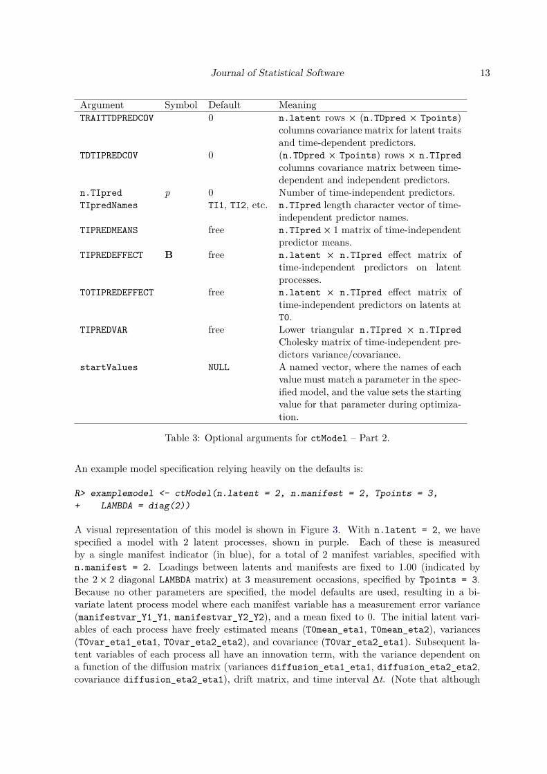
Argument Symbol Default MeaningTRAITTDPREDCOV 0 n.latent rows × (n.TDpred × Tpoints)
columns covariance matrix for latent traitsand time-dependent predictors.
TDTIPREDCOV 0 (n.TDpred × Tpoints) rows × n.TIpredcolumns covariance matrix between time-dependent and independent predictors.
n.TIpred p 0 Number of time-independent predictors.TIpredNames TI1, TI2, etc. n.TIpred length character vector of time-
independent predictor names.TIPREDMEANS free n.TIpred × 1 matrix of time-independent
predictor means.TIPREDEFFECT B free n.latent × n.TIpred effect matrix of
time-independent predictors on latentprocesses.
T0TIPREDEFFECT free n.latent × n.TIpred effect matrix oftime-independent predictors on latents atT0.
TIPREDVAR free Lower triangular n.TIpred × n.TIpredCholesky matrix of time-independent pre-dictors variance/covariance.
startValues NULL A named vector, where the names of eachvalue must match a parameter in the spec-ified model, and the value sets the startingvalue for that parameter during optimiza-tion.
Table 3: Optional arguments for ctModel – Part 2.
An example model specification relying heavily on the defaults is:
R> examplemodel <- ctModel(n.latent = 2, n.manifest = 2, Tpoints = 3,+ LAMBDA = diag(2))
A visual representation of this model is shown in Figure 3. With n.latent = 2, we havespecified a model with 2 latent processes, shown in purple. Each of these is measuredby a single manifest indicator (in blue), for a total of 2 manifest variables, specified withn.manifest = 2. Loadings between latents and manifests are fixed to 1.00 (indicated bythe 2 × 2 diagonal LAMBDA matrix) at 3 measurement occasions, specified by Tpoints = 3.Because no other parameters are specified, the model defaults are used, resulting in a bi-variate latent process model where each manifest variable has a measurement error variance(manifestvar_Y1_Y1, manifestvar_Y2_Y2), and a mean fixed to 0. The initial latent vari-ables of each process have freely estimated means (T0mean_eta1, T0mean_eta2), variances(T0var_eta1_eta1, T0var_eta2_eta2), and covariance (T0var_eta2_eta1). Subsequent la-tent variables of each process all have an innovation term, with the variance dependent ona function of the diffusion matrix (variances diffusion_eta1_eta1, diffusion_eta2_eta2,covariance diffusion_eta2_eta1), drift matrix, and time interval ∆t. (Note that although

14 ctsem: Continuous Time Structural Equation Modeling in R
Figure 3: A two process continuous time model with manifest indicators (blue) measuringlatent processes (purple). Variance/covariance paths are in orange, regressions in red. Lightgray paths indicate those that are either fixed to certain values or constrained to other param-eters. Note that the value of the parameters for all paths to latents at time 2 and higher donot directly represent the effect, rather, the effect depends on a function of the shown param-eter and the time interval ∆t. This model includes neither observed or unobserved betweenperson variance, nor any time-dependent predictors. Manifest intercepts are not shown.
we speak here of variance and covariance parameters for the sake of intuitive understand-ing, ctsem works with Cholesky decomposed covariance matrices, discussed in Section 5.0.1.)Each latent variable in our two processes has continuous auto effects on itself according to thedrift_eta1_eta1 and drift_eta2_eta2 parameters (the diagonals of the drift matrix), andcross effects to the other process according to the drift_eta1_eta2 and drift_eta2_eta1parameters (the off diagonals). This drift matrix combines with time interval ∆t to generatethe auto and cross regressions shown in the diagram. As usual, the first process listed inthe parameter name represents the row of the drift matrix, and the second the column, withthe direction of effects flowing from column to row – so the parameter drift_eta1_eta2represents the effect of a change in process 2 on later values of process 1. Each process has a

Journal of Statistical Software 15
continuous intercept, which sets the level to which each process asymptotes. These are fixedto zero by default, as the manifest intercepts (the MANIFESTMEANS matrix) account for nonzero levels, by default. To see the parameter matrices or simply view a model, printing themodel object (e.g., print(examplemodel)) is recommended. To track how these matrices areused within the complete SEM specification, one must first estimate the model (discussed inSection 6), and may then view the A, S, F or M matrices typical to a RAM specificationMcArdle and McDonald (1984) via example1fit$mxobj$A (for the A matrix).
Cholesky decomposed variance/covariance input matricesTo ensure reliable estimation, some parameter transformations have been implemented in ct-sem for the estimation of covariance matrices. Rather than directly operating on covariancematrices, ctsem takes as input Cholesky decomposed covariance matrices, as these allow forunbounded estimation. The Cholesky decomposition is such that the variance/covariancematrix is given by Σ = LL>, where L is lower-triangular. This means that input vari-ance/covariance matrices for ctsem must be lower triangular. The meaning of a 0 in thematrix is the same for both covariance and Cholesky decomposition approaches. An im-portant point to be aware of is that while Cholesky matrices are required as input, forconvenience, the matrices reported in the summary function are full variance/covariance ma-trices. These can be converted to the Cholesky decomposed form using code in the formt(chol(summary(ctfitobj)$varcovmatrix)).While not affecting interpretations of the matrix input or output, internally, by default ct-sem also optimizes over the natural logarithm of the diagonal of the Cholesky factor covari-ance matrices. These transformations are reflected in the raw OpenMx parameter outputsection of the output summary (when verbose = TRUE), but otherwise require no specificknowledge or action – the logarithmic transformations take place internally, and the regularvariance/covariance matrices are displayed in the summary matrices.
6. Model estimationThe ctFit function estimates the specified model, calling the data in wide format along withthe ctsem model object. For an example, we can fit a similar model to that defined in Section5. We first load an example data set contained in the ctsem package, then use the ctFitfunction for parameter estimation. Output information can be obtained via the summaryfunction. The data set used in this example, is a simulation of the relation between leisuretime and happiness for 100 individuals across 6 measurement occasions. Because our data heredoes not use the default manifest variable names of Y1 and Y2, but rather LeisureTime andHappiness, we must include a manifestNames character vector in our model specification.Because each manifest directly measures a latent process, we can use the same character vectorfor the latentNames argument, though one could specify any character vector of length 2 here,or rely on the defaults of eta1 and eta2.
R> data("ctExample1", package = "ctsem")R> example1model <- ctModel(n.latent = 2, n.manifest = 2, Tpoints = 6,+ manifestNames = c("LeisureTime", "Happiness"),+ latentNames = c("LeisureTime", "Happiness"), LAMBDA = diag(2))R> example1fit <- ctFit(datawide = ctExample1, ctmodelobj = example1model)
16 ctsem: Continuous Time Structural Equation Modeling in R
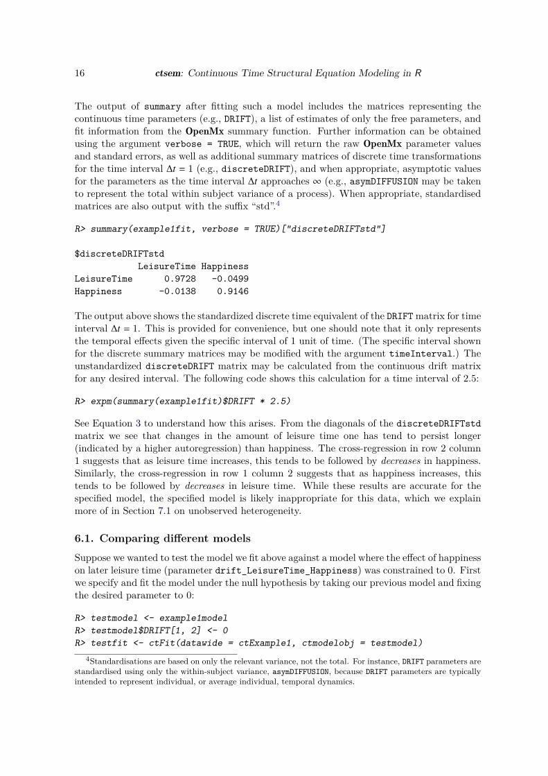
The output of summary after fitting such a model includes the matrices representing thecontinuous time parameters (e.g., DRIFT), a list of estimates of only the free parameters, andfit information from the OpenMx summary function. Further information can be obtainedusing the argument verbose = TRUE, which will return the raw OpenMx parameter valuesand standard errors, as well as additional summary matrices of discrete time transformationsfor the time interval ∆t = 1 (e.g., discreteDRIFT), and when appropriate, asymptotic valuesfor the parameters as the time interval ∆t approaches ∞ (e.g., asymDIFFUSION may be takento represent the total within subject variance of a process). When appropriate, standardisedmatrices are also output with the suffix “std”.4
R> summary(example1fit, verbose = TRUE)["discreteDRIFTstd"]
$discreteDRIFTstdLeisureTime Happiness
LeisureTime 0.9728 -0.0499Happiness -0.0138 0.9146
The output above shows the standardized discrete time equivalent of the DRIFT matrix for timeinterval ∆t = 1. This is provided for convenience, but one should note that it only representsthe temporal effects given the specific interval of 1 unit of time. (The specific interval shownfor the discrete summary matrices may be modified with the argument timeInterval.) Theunstandardized discreteDRIFT matrix may be calculated from the continuous drift matrixfor any desired interval. The following code shows this calculation for a time interval of 2.5:
R> expm(summary(example1fit)$DRIFT * 2.5)
See Equation 3 to understand how this arises. From the diagonals of the discreteDRIFTstdmatrix we see that changes in the amount of leisure time one has tend to persist longer(indicated by a higher autoregression) than happiness. The cross-regression in row 2 column1 suggests that as leisure time increases, this tends to be followed by decreases in happiness.Similarly, the cross-regression in row 1 column 2 suggests that as happiness increases, thistends to be followed by decreases in leisure time. While these results are accurate for thespecified model, the specified model is likely inappropriate for this data, which we explainmore of in Section 7.1 on unobserved heterogeneity.
6.1. Comparing different models
Suppose we wanted to test the model we fit above against a model where the effect of happinesson later leisure time (parameter drift_LeisureTime_Happiness) was constrained to 0. Firstwe specify and fit the model under the null hypothesis by taking our previous model and fixingthe desired parameter to 0:
R> testmodel <- example1modelR> testmodel$DRIFT[1, 2] <- 0R> testfit <- ctFit(datawide = ctExample1, ctmodelobj = testmodel)
4Standardisations are based on only the relevant variance, not the total. For instance, DRIFT parameters arestandardised using only the within-subject variance, asymDIFFUSION, because DRIFT parameters are typicallyintended to represent individual, or average individual, temporal dynamics.

Journal of Statistical Software 17
The result may then be compared to the original model with a likelihood ratio test, using theOpenMx function mxCompare. To use this function a base model fit object and a comparisonmodel fit object must be specified, with the latter being a constrained version of the former.Note that ctsem stores the original OpenMx fit object under a $mxobj sub-object, which mustbe referenced when using OpenMx functions directly.
R> mxCompare(example1fit$mxobj, testfit$mxobj)
base comparison ep minus2LL df AIC diffLL diffdf p1 ctsem <NA> 16 4177 1184 1809 NA NA NA2 ctsem ctsem 15 4197 1185 1827 19.9 1 0.00000833
According to the conventional p < 0.05 criterion, results show that the more constrained modelfits the data significantly worse, that is, happiness has a significant effect on later leisure timefor this model and data. An alternative to this approach is to estimate 95% profile-likelihoodconfidence intervals for our parameters of interest, from our already fit model:
R> example1cifit <- ctCI(example1fit, confidenceintervals = "DRIFT")
lbound estimate ubound notedrift_LeisureTime_LeisureTime -0.0468 -0.0280 -0.0125drift_LeisureTime_Happiness -0.1083 -0.0697 -0.0377drift_Happiness_LeisureTime -0.0312 -0.0111 0.0087drift_Happiness_Happiness -0.1486 -0.0896 -0.0459
Now the summary function reports 95% confidence bounds for the continuous drift param-eters, which in case of drift_Happiness_LeisureTime (DRIFT[1, 2]) does not include 0.For complicated models, the estimation of confidence intervals may increase computationtime considerably. One could also compute a confidence interval by multiplying the standarderror of the estimate (returned in the summary) by 1.96, however profile-likelihood confidenceintervals are in general recommended as they do not assume symmetric intervals, which maybe quite unlikely for such models. We have observed, however, that optimization difficultiescan sometimes result in inacccurate (extremely close to the point estimate, accuracy can bechecked in the lower and upper delta returned by example1cifit$mxobj$intervals sub-object) or missing profile-likelihood confidence intervals, so the use of standard error basedintervals can provide a helpful sanity check.
6.2. Plots
A visual depiction of the relationships between the processes over time is given by the plotmethod for ‘ctsemFit’ objects, i.e., for any fit object created by ctFit. Depending on ar-guments, this function can show the processes’ mean trajectories, within-subject variance,autoregression, and cross regression plots, as well as plots showing expected changes in eachprocess given either an observed change of 1.00, or an exogenous input of 1.00. (The formeris a mixture of the DIFFUSION and DRIFT matrices, while the latter is just an alternativerepresentation of the auto and cross regression plots.) Autoregression plots show the impactof a 1 unit change in a process on later values of that process, while cross regression plots
18 ctsem: Continuous Time Structural Equation Modeling in R
show the impact of a 1 unit change in one process on later values of other processes. Someexamples can be seen in Figure 4.
7. Continuous time models: Extensions
7.1. Unobserved heterogeneity
Traits at the latent level
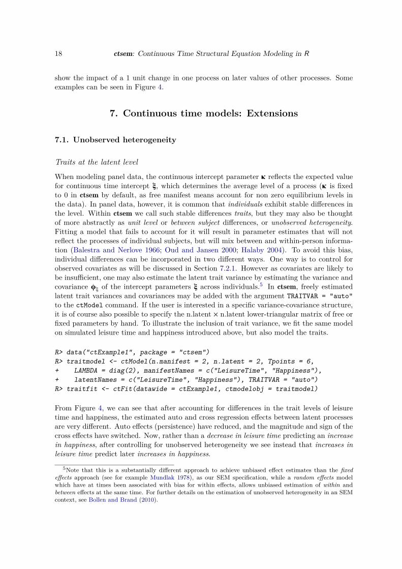
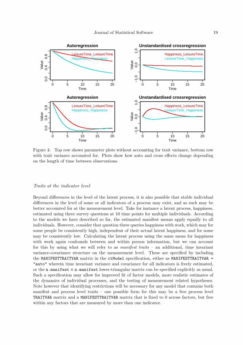
When modeling panel data, the continuous intercept parameter κ reflects the expected valuefor continuous time intercept ξ, which determines the average level of a process (κ is fixedto 0 in ctsem by default, as free manifest means account for non zero equilibrium levels inthe data). In panel data, however, it is common that individuals exhibit stable differences inthe level. Within ctsem we call such stable differences traits, but they may also be thoughtof more abstractly as unit level or between subject differences, or unobserved heterogeneity.Fitting a model that fails to account for it will result in parameter estimates that will notreflect the processes of individual subjects, but will mix between and within-person informa-tion (Balestra and Nerlove 1966; Oud and Jansen 2000; Halaby 2004). To avoid this bias,individual differences can be incorporated in two different ways. One way is to control forobserved covariates as will be discussed in Section 7.2.1. However as covariates are likely tobe insufficient, one may also estimate the latent trait variance by estimating the variance andcovariance φξ of the intercept parameters ξ across individuals.5 In ctsem, freely estimatedlatent trait variances and covariances may be added with the argument TRAITVAR = "auto"to the ctModel command. If the user is interested in a specific variance-covariance structure,it is of course also possible to specify the n.latent × n.latent lower-triangular matrix of free orfixed parameters by hand. To illustrate the inclusion of trait variance, we fit the same modelon simulated leisure time and happiness introduced above, but also model the traits.
R> data("ctExample1", package = "ctsem")R> traitmodel <- ctModel(n.manifest = 2, n.latent = 2, Tpoints = 6,+ LAMBDA = diag(2), manifestNames = c("LeisureTime", "Happiness"),+ latentNames = c("LeisureTime", "Happiness"), TRAITVAR = "auto")R> traitfit <- ctFit(datawide = ctExample1, ctmodelobj = traitmodel)
From Figure 4, we can see that after accounting for differences in the trait levels of leisuretime and happiness, the estimated auto and cross regression effects between latent processesare very different. Auto effects (persistence) have reduced, and the magnitude and sign of thecross effects have switched. Now, rather than a decrease in leisure time predicting an increasein happiness, after controlling for unobserved heterogeneity we see instead that increases inleisure time predict later increases in happiness.
5Note that this is a substantially different approach to achieve unbiased effect estimates than the fixedeffects approach (see for example Mundlak 1978), as our SEM specification, while a random effects modelwhich have at times been associated with bias for within effects, allows unbiased estimation of within andbetween effects at the same time. For further details on the estimation of unobserved heterogeneity in an SEMcontext, see Bollen and Brand (2010).
Journal of Statistical Software 19
0 5 10 15 20
0.0
0.4
0.8
Autoregression
Time
Val
ue
LeisureTime_LeisureTimeHappiness_Happiness
0 5 10 15 20
−1.
00.
01.
0
Unstandardised crossregression
Time
Val
ue
Happiness_LeisureTimeLeisureTime_Happiness
0 5 10 15 20
0.0
0.4
0.8
Autoregression
Time
Val
ue
LeisureTime_LeisureTimeHappiness_Happiness
0 5 10 15 20−
1.0
0.0
1.0
Unstandardised crossregression
Time
Val
ue
Happiness_LeisureTimeLeisureTime_Happiness
Figure 4: Top row shows parameter plots without accounting for trait variance, bottom rowwith trait variance accounted for. Plots show how auto and cross effects change dependingon the length of time between observations.
Traits at the indicator level
Beyond differences in the level of the latent process, it is also possible that stable individualdifferences in the level of some or all indicators of a process may exist, and as such may bebetter accounted for at the measurement level. Take for instance a latent process, happiness,estimated using three survey questions at 10 time points for multiple individuals. Accordingto the models we have described so far, the estimated manifest means apply equally to allindividuals. However, consider that question three queries happiness with work, which may forsome people be consistently high, independent of their actual latent happiness, and for somemay be consistently low. Calculating the latent process using the same mean for happinesswith work again confounds between and within person information, but we can accountfor this by using what we will refer to as manifest traits – an additional, time invariantvariance-covariance structure on the measurement level. These are specified by includingthe MANIFESTTRAITVAR matrix in the ctModel specification, either as MANIFESTTRAITVAR ="auto" wherein time invariant variance and covariance for all indicators is freely estimated,or the n.manifest × n.manifest lower-triangular matrix can be specified explicitly as usual.Such a specification may allow for improved fit of factor models, more realistic estimates ofthe dynamics of individual processes, and the testing of measurement related hypotheses.Note however that identifying restrictions will be necessary for any model that contains bothmanifest and process level traits – one possible form for this may be a free process levelTRAITVAR matrix and a MANIFESTTRAITVAR matrix that is fixed to 0 across factors, but freewithin any factors that are measured by more than one indicator.

20 ctsem: Continuous Time Structural Equation Modeling in R
7.2. Predictors
ctsem allows the inclusion of time-independent as well as time-dependent exogenous predic-tors. Time-independent predictors could be variables such as gender, personality or socio-demographic background variables that remain constant over time. An example of a time-dependent predictor could be a financial crisis, which all individuals in the sample experienceat the same time, or the death of a loved one, which only some individuals may experienceand for whom the time point of the event may differ. Both events may be thought of asadding some relatively distinct and sudden change to an individual’s life, which influencesthe processes of interest. Time-dependent predictors are distinguished from the endogenouslatent processes in that they are assumed to be independent of fluctuations in the processes –changes in the latent processes do not lead to changes in the predictor. Furthermore, no tem-poral structure between different time points is modeled. Because of these two assumptions,in any case where the time-dependent predictor depends on earlier values of either itself orthe latent process, it may be better to model it as an additional latent process.
Time-independent predictors
Time-independent predictors are added by including the data as per the structures shownin Section 4, and specifying the number of time independent predictors, n.TIpred, in thectModel arguments. If not using the default variable naming, a TIpredNames character vectorshould also be specified. For an example, we add the “number of close friends” as a time-independent predictor to the earlier leisure time and happiness model. Note that, just like inany conventional regression analysis, if time-independent predictors are not centered around0, the estimate of continuous intercept parameters depends on the mean of the predictor.
R> data("ctExample1TIpred", package = "ctsem")R> tipredmodel <- ctModel(n.manifest = 2, n.latent = 2, n.TIpred = 1,+ manifestNames = c("LeisureTime", "Happiness"),+ latentNames = c("LeisureTime", "Happiness"),+ TIpredNames = "NumFriends", Tpoints = 6, LAMBDA = diag(2),+ TRAITVAR = "auto")R> tipredfit <- ctFit(datawide = ctExample1TIpred, ctmodelobj = tipredmodel)R> summary(tipredfit, verbose = TRUE)["TIPREDEFFECT"]R> summary(tipredfit, verbose = TRUE)["discreteTIPREDEFFECT"]R> summary(tipredfit, verbose = TRUE)["asymTIPREDEFFECT"]R> summary(tipredfit, verbose = TRUE)["addedTIPREDVAR"]
$TIPREDEFFECTNumFriends
LeisureTime -0.225Happiness 0.549
$discreteTIPREDEFFECTNumFriends
LeisureTime -0.239Happiness 0.442

Journal of Statistical Software 21
$asymTIPREDEFFECTNumFriends
LeisureTime -1.673Happiness 0.219
$addedTIPREDVARLeisureTime Happiness
LeisureTime 2.838 -0.3719Happiness -0.372 0.0487
The matrices output from summary, verbose = TRUE will now include matrices related totime-independent predictors, while the estimated parameters now also includes a range of vari-ance, covariance, and effect parameters for time-independent predictors. Matrix TIPREDEFFECTdisplays the continuous time effect parameters, however discreteTIPREDEFFECT shows theeffect added to the processes for each unit of time, which may provide a useful comparisonwith discrete time models. asymTIPREDEFFECT (asymptotic time-independent predictor ef-fect) shows the expected total change in process means given an increase of 1 on the timeindependent predictor. From these matrices we see that the number of close friends hasa negative relationship to leisure time, but a positive relationship to happiness. The finalmatrix, addedTIPREDVAR, displays the stable between-subject variance and covariance in theprocesses accounted for by the time-independent predictors.
Time-dependent predictors
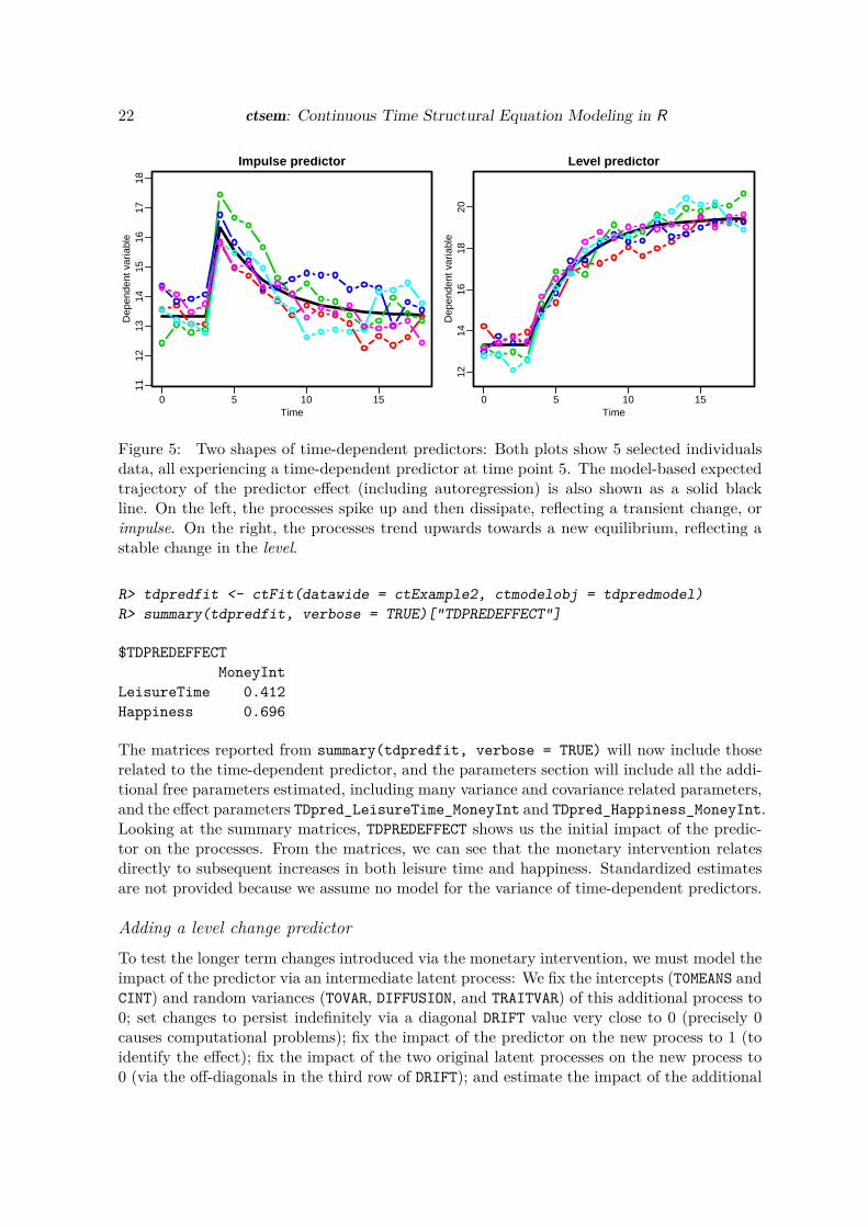
ctsem allows the specification of time-dependent predictors: The fundamental form of sucha predictor is that of a sudden impulse to the system which then dissipates back to theprocess mean, however with some thought it is possible to specify a wide range of effectshapes. Figure 5 provides an example of two different extremes, the basic impulse form anda permanent level change form.A single time-dependent predictor can be incorporated in a ctsem model by adding the argu-ment n.TDpred = 1 to the ctModel function, as well as a TDpredNames vector if not using thedefault variable naming in your data, then fitting as usual. In the following example, we usethe same two simulated processes as above and include an intervention that all individualsexperience at time 5. For example, let us assume everyone receives a large amount of moneyand we are interested in the impact of this monetary gift on leisure time and happiness. Weexpect that some short term increase in both leisure time and happiness may occur, as peoplemay take holidays or enjoy the unexpected boon otherwise, but we also want to check whetherthe gift we provide may also cause a longer term adjustment in leisure time or happiness. Tothis end we first fit a model with the basic impulse effect, coded in the data as a 1 when theintervention occurs and a 0 otherwise.6
R> data("ctExample2", package = "ctsem")R> tdpredmodel <- ctModel(n.manifest = 2, n.latent = 2, n.TDpred = 1,+ Tpoints = 8, manifestNames = c("LeisureTime", "Happiness"),+ TDpredNames = "MoneyInt", latentNames = c("LeisureTime", "Happiness"),+ LAMBDA = diag(2), TRAITVAR = "auto")
6While this form of dummy coding works well, if there are predictors with no variance and the TDPREDVARmatrix is not specified, ctsem warns the user and fixes TDPREDVAR to a diagonal matrix with small variance.
22 ctsem: Continuous Time Structural Equation Modeling in R
0 5 10 15
1112
1314
1516
1718
Impulse predictor
Time
Dep
ende
nt v
aria
ble
0 5 10 15
1214
1618
20
Level predictor
Time
Dep
ende
nt v
aria
ble
Figure 5: Two shapes of time-dependent predictors: Both plots show 5 selected individualsdata, all experiencing a time-dependent predictor at time point 5. The model-based expectedtrajectory of the predictor effect (including autoregression) is also shown as a solid blackline. On the left, the processes spike up and then dissipate, reflecting a transient change, orimpulse. On the right, the processes trend upwards towards a new equilibrium, reflecting astable change in the level.
R> tdpredfit <- ctFit(datawide = ctExample2, ctmodelobj = tdpredmodel)R> summary(tdpredfit, verbose = TRUE)["TDPREDEFFECT"]
$TDPREDEFFECTMoneyInt
LeisureTime 0.412Happiness 0.696
The matrices reported from summary(tdpredfit, verbose = TRUE) will now include thoserelated to the time-dependent predictor, and the parameters section will include all the addi-tional free parameters estimated, including many variance and covariance related parameters,and the effect parameters TDpred_LeisureTime_MoneyInt and TDpred_Happiness_MoneyInt.Looking at the summary matrices, TDPREDEFFECT shows us the initial impact of the predic-tor on the processes. From the matrices, we can see that the monetary intervention relatesdirectly to subsequent increases in both leisure time and happiness. Standardized estimatesare not provided because we assume no model for the variance of time-dependent predictors.
Adding a level change predictorTo test the longer term changes introduced via the monetary intervention, we must model theimpact of the predictor via an intermediate latent process: We fix the intercepts (T0MEANS andCINT) and random variances (T0VAR, DIFFUSION, and TRAITVAR) of this additional process to0; set changes to persist indefinitely via a diagonal DRIFT value very close to 0 (precisely 0causes computational problems); fix the impact of the predictor on the new process to 1 (toidentify the effect); fix the impact of the two original latent processes on the new process to0 (via the off-diagonals in the third row of DRIFT); and estimate the impact of the additional

Journal of Statistical Software 23
process on our original two processes of interest (via the off-diagonals in the third column ofDRIFT). Alternatively, one could also estimate the time course of predictor effects by freeingthe DRIFT diagonal of the additional process.
R> data("ctExample2", package = "ctsem")R> tdpredlevelmodel <- ctModel(n.manifest = 2, n.latent = 3, n.TDpred = 1,+ Tpoints = 8, manifestNames = c("LeisureTime", "Happiness"),+ TDpredNames = "MoneyInt",+ latentNames = c("LeisureTime", "Happiness", "MoneyIntLatent"),+ LAMBDA = matrix(c(1, 0, 0, 1, 0, 0), ncol = 3), TRAITVAR = "auto")R> tdpredlevelmodel$TRAITVAR[3, ] <- 0R> tdpredlevelmodel$TRAITVAR[, 3] <- 0R> tdpredlevelmodel$DIFFUSION[, 3] <- 0R> tdpredlevelmodel$DIFFUSION[3, ] <- 0R> tdpredlevelmodel$T0VAR[3, ] <- 0R> tdpredlevelmodel$T0VAR[, 3] <- 0R> tdpredlevelmodel$CINT[3] <- 0R> tdpredlevelmodel$T0MEANS[3] <- 0R> tdpredlevelmodel$TDPREDEFFECT[1:3, ] <- c(0, 0, 1)R> tdpredlevelmodel$DRIFT[3, ] <- c(0, 0, -0.000001)R> tdpredlevelfit <- ctFit(datawide = ctExample2,+ ctmodelobj = tdpredlevelmodel)R> summary(tdpredlevelfit, verbose = TRUE)[c("DRIFT", "TDPREDEFFECT")]
$DRIFTLeisureTime Happiness MoneyIntLatent
LeisureTime -0.1393 -0.0394 0.569907Happiness 0.0798 -0.1038 -0.357674MoneyIntLatent 0.0000 0.0000 -0.000001
$TDPREDEFFECTMoneyInt
LeisureTime 0Happiness 0MoneyIntLatent 1
Now, if we look at column 3 of the DRIFT matrix, we see that the monetary interventionprocess appears to cause long term increases in leisure time, but potentially reductions inhappiness.
7.3. N = 1 time series with multiple indicators
In the examples so far, we have dealt with multiple individuals with relatively few measure-ment occasions, and latent processes have been estimated by a single indicator. However,ctsem may also be used for the analysis of time series data for single subjects observed atmany measurement occasions, as well as the estimation of latent factors estimated from mul-tiple indicators. With single-subject data, a Kalman filter implementation is typically far

24 ctsem: Continuous Time Structural Equation Modeling in R
quicker than the matrix arrangement we use for multiple subjects, however ctsem allows ei-ther to be used. To illustrate these features, we perform a dynamic factor analysis on a singleindividual, with three manifest indicators measured at 50 occasions. Because the model isfitted to a single individual, we cannot freely estimate both the latent variance and meanat the first measurement occasion, but we must fix the 1 × 1 T0VAR matrix to a reasonablevalue, or implement stationarity constraints as discussed in Section 4.3. The precise fixedvalue becomes unimportant as the time series length increases (Durbin and Koopman 2012).Note that in this example the LAMBDA matrix specifies a loading of 1.00 for manifest Y1 (foridentification), while loadings for Y2 and Y3 are freely estimated. Note also that althoughctsem uses the Kalman filter by default when a single subject is specified, this can be over-ridden by specifying the objective = "mxRAM" argument to ctFit, if one wishes to use theslower RAM implementation. The Kalman filter may also be specified for multiple subjects.In this case, between subject trait or time independent predictor matrices are ignored – onemay need to account for consistent differences between subjects through pre-processing orthoughtful expansion of the state matrices.
R> data("ctExample3", package = "ctsem")R> model <- ctModel(n.latent = 1, n.manifest = 3, Tpoints = 100,+ LAMBDA = matrix(c(1, "lambda2", "lambda3"), nrow = 3, ncol = 1),+ MANIFESTMEANS = matrix(c(0, "manifestmean2", "manifestmean3"),+ nrow = 3, ncol = 1))R> fit <- ctFit(data = ctExample3, ctmodelobj = model, objective = "Kalman",+ stationary = "T0VAR")
7.4. Multiple group continuous time models
In some cases, certain groups or individuals may exhibit different model parameters. We caninvestigate group or individual level differences by specifying a multiple group model using thectMultigroupFit function. For this example, we will use the same model structure as in thesingle subject example from Section 7.3, but apply it to two groups of 10 individuals, whomwe expect to exhibit differences in the loading of the third manifest variable. When usingctMultigroupFit, all parameters are free across groups by default. However, in addition tothe standard model specification you may also specify either a fixed model, or a free model.A fixed model should be of the same structure as the base model, with any parametersyou wish to constrain across groups set to the character string “groupfixed”. The value forany other parameters is not important. Alternatively, one may specify a free model, whereany parameters to freely estimate for each group are given the label “groupfree”, and allothers will be constrained across groups. In this example, because we only want to examinegroup differences on one parameter, we specify a free model in which the loading parameterbetween manifest3 and our latent process eta1 is labeled “groupfree” – this estimates distinctlambda3 parameters for each group, and constrains all other parameters across the two groupsto equality. The group specific parameter estimates will appear in the resulting summaryprefixed by the specified grouping vector. This is the final requirement for ctMultigroupFitand is simply a vector specifying a group label for each row of our data. In this case we havegroups one and two, containing the first and the last 10 rows of data respectively, prefixed bythe letter “g” to denote group.
Journal of Statistical Software 25
R> data("ctExample4", package = "ctsem")R> basemodel <- ctModel(n.latent = 1, n.manifest = 3, Tpoints = 20,+ LAMBDA = matrix(c(1, "lambda2", "lambda3"), nrow = 3, ncol = 1),+ MANIFESTMEANS = matrix(c(0, "manifestmean2", "manifestmean3"),+ nrow = 3, ncol = 1))R> freemodel <- basemodelR> freemodel$LAMBDA[3, 1] <- "groupfree"R> groups <- paste0("g", rep(1:2, each = 10))R> multif <- ctMultigroupFit(datawide = ctExample4, groupings = groups,+ objective = "Kalman", ctmodelobj = basemodel, freemodel = freemodel)
g1_lambda3 g2_lambda31.417 0.208
Looking at the estimated parameters from the $omxsummary (OpenMx) portion of summary,verbose = TRUE, we indeed see a difference between parameters g1_lambda3 (group 1) andg2_lambda3 (group 2), and could test this with the usual approaches discussed in Section 6.1.A point to note is that the multiple group and Kalman filter implementations can be easilycombined by specifying a distinct group for each row of data. This can allow for a mixtureof individual and group level parameters.
7.5. Higher order models and simulating data
In the models discussed so far, the individual processes were only conceived of as first orderprocesses, always tending to revert to baseline when away from it. However, what abouta situation where we have variables which show very slow patterns of change, upwards ordownwards trajectories that are maintained over many observations? This can provide foroscillations and slower patterns of change, as for example with damped linear oscillators, ormoving average like effects as from the ARMA modeling framework.Continuous time models of this variety are theoretically plausible, as changes to the levelof a process are not necessarily always random in direction with a tendency to baseline, butmay depend on contextual circumstances that have some persistence. Consider an individual’soverall health over the course of 20 years, sampled every few months. If the individual changesexercise or eating habits, changes in health do not manifest instantly, rather we could expecteither a slow increase or slow reduction, depending on whether the change of habits waspositive or negative. Thus, for many measurements, the change in health from the previousmeasurement will likely be in the same direction as the change was one step earlier. Thefollowing details how to specify such a model, generate data using the ctGenerate function,simply plot the generated data, and estimate the parameters.
R> genm <- ctModel(Tpoints = 200, n.latent = 2, n.manifest = 1,+ LAMBDA = matrix(c(1, 0), nrow = 1, ncol = 2),+ DIFFUSION = matrix(c(0, 0, 0, 1), 2),+ MANIFESTVAR = t(chol(diag(.6, 1))),+ DRIFT = matrix(c(0, -0.1, 1, -0.2), nrow = 2),+ CINT = matrix(c(1, 0), nrow = 2))R> data <- ctGenerate(genm, n.subjects = 1, burnin = 200)

26 ctsem: Continuous Time Structural Equation Modeling in R
R> ctIndplot(data, n.subjects = 1 , n.manifest = 1, Tpoints = 200)R> model <- ctModel(Tpoints = 200, n.latent = 2, n.manifest = 1,+ LAMBDA = matrix(c(1, 0), nrow = 1, ncol = 2),+ DIFFUSION = matrix(c(0, 0, 0, "diffusion"), 2),+ DRIFT = matrix(c(0, "regulation", 1, "diffusionAR"), nrow = 2))R> fit <- ctFit(data, model, stationary = "T0VAR")
In the above, we focus on a model for a single subject, and specify with LAMBDA that a singlemanifest variable measures only the first latent process. With DIFFUSION we specify thatonly the 2nd unobserved process experiences random innovations. With DRIFT, we specifythat the 2nd process has a freely estimated autoregression term, that it directly impacts thefirst process with a 1:1 relationship, and that as the level of the first process increases, thelevel of the 2nd process decreases – providing necessary regulation.
Damped linear oscillatorVoelkle and Oud (2013) discuss modeling a damped linear oscillator in detail, however herewe demonstrate how to load the data and fit the oscillating model from their paper. In thiscase, we also specify good starting values with the startValues argument to ctModel, andbecause of this, set the argument carefulFit = FALSE.
R> data("Oscillating", package = "ctsem")R> inits <- c(-39, -0.3, 1.01, 10.01, 0.1, 10.01, 0.05, 0.9, 0)R> names(inits) <- c("crosseffect", "autoeffect", "diffusion",+ "T0var11", "T0var21", "T0var22", "m1", "m2", "manifestmean")R> oscillatingm <- ctModel(n.latent = 2, n.manifest = 1, Tpoints = 11,+ MANIFESTVAR = matrix(0, nrow = 1, ncol = 1),+ LAMBDA = matrix(c(1, 0), nrow = 1, ncol = 2),+ T0MEANS = matrix(c("m1", "m2"), nrow = 2, ncol = 1),+ T0VAR = matrix(c("T0var11", "T0var21", 0, "T0var22"),+ nrow = 2, ncol = 2),+ DRIFT = matrix(c(0, "crosseffect", 1, "autoeffect"),+ nrow = 2, ncol = 2),+ MANIFESTMEANS = matrix("manifestmean", nrow = 1, ncol = 1),+ DIFFUSION = matrix(c(0, 0, 0, "diffusion"), nrow = 2, ncol = 2),+ startValues = inits)R> oscillatingf <- ctFit(Oscillating, oscillatingm, carefulFit = FALSE)
8. Further specification options and tips for model estimationGiven the complexity of parameter constraints, and that for some classes of models multipleminima may exist, parameter estimation is sometimes difficult. To ensure reliable estima-tion, there are some additional approaches that may be helpful. By default the argumentcarefulFit = TRUE for the ctFit function is specified. This initiates a two-step procedure,in which the first step penalizes the likelihood7 to help maintain potentially problematic pa-
7The sum of squares of each parameter that is neither factor loading nor mean related is added to thelikelihood, as is the inverse of any parameters on the diagonals of square matrices – essentially penalizingvalues at the extremes.
Journal of Statistical Software 27
rameters close (but not too close!) to 0, and then uses these estimates as starting values formaximum likelihood estimation. Though often useful, in some cases (particularly those withcomplex dynamics, or user specified starting values) it can help to switch this off. Beyondthis, as a general guideline we suggest starting with simpler, more constrained models andfreeing parameters in a stepwise fashion (not necessary as a means of model development,simply for fitting purposes). The ctRefineTo function can be used as a replacement for ctFitand automates this stepwise progression. One could do this manually by developing the mea-surement model separately, estimating only autoregressive parameters of the DRIFT matrixat first (in simple models, this means constraining the off-diagonals of the DRIFT matrix to0), or fixing the factor loading matrix prior to free estimation. For such stepwise progression,the default of small and negative starting values for cross effects should be switched off byargument crossEffectNegStarts = FALSE, and starting values from the restricted modelshould be obtained via the omxStartValues argument, as shown here, using the model fitfrom from Section 6:
R> omxInits <- omxGetParameters(example1fit$mxobj)R> fitWithInits <- ctFit(data = ctExample1, ctmodelobj = example1model,+ omxStartValues = omxInits)
If stepwise model building with starting values based on simpler fits still fails to producean improved solution, some of the following suggestions may be helpful. The time scale,although theoretically unimportant in the sense that all time ranges can be accounted for,can be computationally relevant. It is helpful to choose a scale that roughly matches theexpected dynamics – for instance a time scale of nanoseconds for panel data measured yearlywould be problematic, instead, a yearly or monthly time scale could be used. Centering thegrand mean of the variables to 0 may help, as can standardizing the variances, particularlyin cases where both a measurement model and dynamic model are estimated. One way tosearch for an improved solution is simply to try many times with varying starting values.This is automated by default using the mxTryHard function from OpenMx, however youmay want to increase the retryattempts argument to ctFit, or simply re-run ctFit manytimes, as it generates unspecified starting values with some limited randomness. However,since both automated procedures begin within a similar range, for truly problematic casesone may consider adding more extensive randomness to the starting values manually. Insituations with a limited number of time points or of high complexity, you may implementthe stationarity assumption, so that parameters related to the first time point are no longerestimated, but constrained to the asymptotic effects, when the time interval ∆t → ∞. Thiscan make optimization more straightforward, and may serve as a useful basis for determiningstarting values, or as a viable model in itself. For more discussion regarding stationarityconditions see Section 4.3. In some cases, optimizing over the continuous time parameters(the default) results in fits that do not pass every check and you may be left with warnings.If this occurs, you can instead optimize over asymptotic variants of the parameters, by usingthe argument asymptotes = TRUE to ctFit. This will in general produce equivalent resultsif the DIFFUSION, CINT, and TIPRED matrices are all freely estimated, even though the rawparameters of these matrices will look different. If these matrices have been constrained insome way, this approach is not recommended.

28 ctsem: Continuous Time Structural Equation Modeling in R
8.1. Optimization performance
When time intervals vary for every individual, optimization can be quite slow. To quicklyestimate approximate versions of a model, you may use the meanIntervals = TRUE argumentto ctFit, which will set every individual’s time intervals to the mean of the interval acrossall individuals. A step further even is to specify the argument objective = "cov" in orderto estimate a covariance matrix from the supplied data and fit directly to that. In cases withvariability in time intervals these approaches will substantially speed up optimization, butalso waste information and bias parameters. Using such an approach in combination with aconstrained DRIFT matrix to generate starting values may be a reasonable way to improvefitting speed and generate starting values for large and complex models.
9. Limitations and future directionsCurrently, a number of assumptions are present in the specification of continuous time modelsimplemented in ctsem. Although the processes are allowed to begin at different levels andvariances, from then on a time-invariant model is assumed. Thus, ctsem cannot presentlyaccount for time-varying aspects of the processes, except in the form of observed exogenousinputs via time-dependent predictors. Although as with many discrete models we could freevarious parameters across measurement occasions, their meaning would become unclear, aseach measurement occasion (set of n.manifest columns in the wide format data) may containobservations from many different times. Instead, models which allow parameters to vary asa function of time could be incorporated in the future as per the time-varying specificationin Oud and Jansen (2000). As we fit using full information maximum likelihood, standardassumptions regarding multivariate normality apply to manifest variables. Generalizations ofthe measurement model to allow for non-normal indicators could be implemented using theregular OpenMx functionality however. Although we allow for heterogeneity in the level ofthe processes across individuals, heterogeneity in other parameters is not accounted for, andcan only be examined via multiple group approaches. Presently, effects are assumed to betransmitted near instantaneously, as we do not estimate a dead time between inputs and theeffect of inputs. We believe this is unlikely to severely impact estimates unless the dead timeis of a similar or greater order of magnitude as the time course of effects, however such aparameter could potentially be incorporated within the continuous time equations (Richard2003). Although in such areas ctsem may benefit from expansion, ctsem as it stands allowsfor the straightforward specification of continuous time dynamic models for both panel andtime series data, which may include a measurement model, exogenous predictors, multipleprocesses, unobserved heterogeneity, multiple groups, as well as easy to specify parameterconstraints and more complex dynamic specifications.
AcknowledgmentsWe would like to thank the Intra Person Dynamics and the Formal Methods research groupsat the Max Planck Institute for Human Development for assistance with this work, as wellas Joshua Pritikin and the OpenMx development team for feedback and fast response toissues. The knitr (Xie 2015) and Ωnyx (von Oertzen, Brandmaier, and Tsang 2015) softwarepackages were invaluable in constructing this document.

Journal of Statistical Software 29
References
Arnold L (1974). Stochastic Differential Equations: Theory and Applications. John Wiley &Sons, New York.
Balestra P, Nerlove M (1966). “Pooling Cross Section and Time Series Data in the Estimationof a Dynamic Model: The Demand for Natural Gas.” Econometrica, 34(3), 585–612. doi:10.2307/1909771.
Bollen KA, Brand JE (2010). “A General Panel Model with Random and Fixed Effects: AStructural Equations Approach.” Social Forces, 89(1), 1–34. doi:10.1353/sof.2010.0072.
Brouste A, Fukasawa M, Hino H, Iacus SM, Kamatani K, Koike Y, Masuda H, Nomura R,Ogihara T, Shimuzu Y, Uchida M, Yoshida N (2014). “The YUIMA Project: A Com-putational Framework for Simulation and Inference of Stochastic Differential Equations.”Journal of Statistical Software, 57(4), 1–51. doi:10.18637/jss.v057.i04.
Canova F, Ciccarelli M, Ortega E (2012). “Do Institutional Changes Affect Business Cycles?Evidence from Europe.” Journal of Economic Dynamics and Control, 36(10), 1520–1533.doi:10.1016/j.jedc.2012.03.017.
Chow SM, Ho MhR, Hamaker EL, Dolan CV (2010). “Equivalence and Differences be-tween Structural Equation Modeling and State-Space Modeling Techniques.” Struc-tural Equation Modeling: A Multidisciplinary Journal, 17(2), 303–332. doi:10.1080/10705511003661553.
Coleman JS (1964). Introduction to Mathematical Sociology. London Free Press Glencoe.
Driver C, Voelkle M, Oud H (2017). ctsem: Continuous Time Structural Equation Modelling.R package version 2.3.0, URL https://CRAN.R-project.org/package=ctsem.
Durbin J, Koopman SJ (2012). Time Series Analysis by State Space Methods. 2nd edition.Oxford University Press.
Ghisletta P, Lindenberger U (2005). “Exploring Structural Dynamics within and BetweenSensory and Intellectual Functioning in Old and Very Old Age: Longitudinal Evidencefrom the Berlin Aging Study.” Intelligence, 33(6), 555–587. doi:10.1016/j.intell.2005.07.002.
Gill P, Murray W, Saunders M, Wright M (2001). NPSOL: A Fortran Package for Non-linear Programming. Version 5.0, URL http://www.sbsi-sol-optimize.com/asp/sol_product_npsol.htm.
Grijalva CG, Nuorti JP, Arbogast PG, Martin SW, Edwards KM, Griffin MR (2007). “Declinein Pneumonia Admissions After Routine Childhood Immunisation with Pneumococcal Con-jugate Vaccine in the USA: A Time-Series Analysis.” The Lancet, 369(9568), 1179–1186.doi:10.1016/S0140-6736(07)60564-9.
Guidoum AC, Boukhetala K (2017). Sim.DiffProc: Simulation of Diffusion Processes. Rpackage version 3.7, URL https://CRAN.R-project.org/package=Sim.DiffProc.

30 ctsem: Continuous Time Structural Equation Modeling in R
Halaby CN (2004). “Panel Models in Sociological Research: Theory into Practice.” AnnualReview of Sociology, 30(1), 507–544. doi:10.1146/annurev.soc.30.012703.110629.
Hannan MT, Tuma NB (1979). “Methods for Temporal Analysis.” Annual Review of Sociology,5(1), 303–328. doi:10.1146/annurev.so.05.080179.001511.
Helgason T, Tomasson H, Zoega T (2004). “Antidepressants and Public Health in Iceland.”The British Journal of Psychiatry, 184(2), 157–162. doi:10.1192/bjp.184.2.157.
Higham N (2009). “The Scaling and Squaring Method for the Matrix Exponential Revisited.”SIAM Review, 51(4), 747–764. doi:10.1137/090768539.
Hunter MD (2014). State Space Dynamic Mixture Modeling: Finding People with SimilarPatterns Of Change. Ph.D. thesis, University of Oklahoma, Norman, OK.
Iacus SM (2016). sde: Simulation and Inference for Stochastic Differential Equations. Rpackage version 2.0.15, URL https://CRAN.R-project.org/package=sde.
Keijsers L, Loeber R, Branje S, Meeus W (2011). “Bidirectional Links and Concurrent Devel-opment of Parent-Child Relationships and Boys’ Offending Behavior.” Journal of AbnormalPsychology, 120(4), 878–889. doi:10.1037/a0024588.
King AA, Nguyen D, Ionides EL (2016). “Statistical Inference for Partially Observed MarkovProcesses via the R Package pomp.” Journal of Statistical Software, 69(12), 1–43. doi:10.18637/jss.v069.i12.
McArdle JJ, McDonald RP (1984). “Some Algebraic Properties of the Reticular Action Modelfor Moment Structures.” British Journal of Mathematical and Statistical Psychology, 37(2),234–251. doi:10.1111/j.2044-8317.1984.tb00802.x.
Mundlak Y (1978). “On the Pooling of Time Series and Cross Section Data.” Econometrica,46(1), 69–85. doi:10.2307/1913646.
Neale MC, Hunter MD, Pritikin JN, Zahery M, Brick TR, Kirkpatrick RM, Estabrook R,Bates TC, Maes HH, Boker SM (2016). “OpenMx 2.0: Extended Structural Equation andStatistical Modeling.” Psychometrika, 81(2), 535–549. doi:10.1007/s11336-014-9435-8.
Oud JHL (2002). “Continuous Time Modeling of the Cross-Lagged Panel Design.” Kwanti-tatieve Methoden, 69(1), 1–26.
Oud JHL, Jansen RARG (2000). “Continuous Time State Space Modeling of Panel Data byMeans of SEM.” Psychometrika, 65(2), 199–215. doi:10.1007/BF02294374.
R Core Team (2017). R: A Language and Environment for Statistical Computing. R Founda-tion for Statistical Computing, Vienna, Austria. URL https://www.R-project.org/.
Richard JP (2003). “Time-Delay Systems: An Overview of Some Recent Advances and OpenProblems.” Automatica, 39(10), 1667–1694. doi:10.1016/S0005-1098(03)00167-5.
Rindskopf D (1984). “Using Phantom and Imaginary Latent Variables to Parameter-ize Constraints in Linear Structural Models.” Psychometrika, 49(1), 37–47. doi:10.1007/BF02294204.
Journal of Statistical Software 31
Singer H (1998). “Continuous Panel Models with Time Dependent Parameters.” Journal ofMathematical Sociology, 23(2), 77–98. doi:10.1080/0022250X.1998.9990214.
Voelkle MC, Oud JHL (2013). “Continuous Time Modelling with Individually Varying TimeIntervals for Oscillating and Non-Oscillating Processes.” British Journal of Mathematicaland Statistical Psychology, 66(1), 103–126. doi:10.1111/j.2044-8317.2012.02043.x.
Voelkle MC, Oud JHL (2015). “Relating Latent Change Score and Continuous Time Models.”Structural Equation Modeling: A Multidisciplinary Journal, 22(3), 366–381. doi:10.1080/10705511.2014.935918.
Voelkle MC, Oud JHL, Davidov E, Schmidt P (2012). “An SEM Approach to ContinuousTime Modeling of Panel Data: Relating Authoritarianism and Anomia.” PsychologicalMethods, 17(2), 176–192. doi:10.1037/a0027543.
von Oertzen T, Brandmaier AM, Tsang S (2015). “Structural Equation Modeling with Ωnyx.”Structural Equation Modeling: A Multidisciplinary Journal, 22(1), 148–161. doi:10.1080/10705511.2014.935842.
Wang Z (2013). “cts: An R Package for Continuous Time Autoregressive Models via KalmanFilter.” Journal of Statistical Software, 53(5), 1–19. doi:10.18637/jss.v053.i05.
Xie Y (2015). Dynamic Documents with R and knitr. 2nd edition. Chapman & Hall/CRC,Boca Raton.
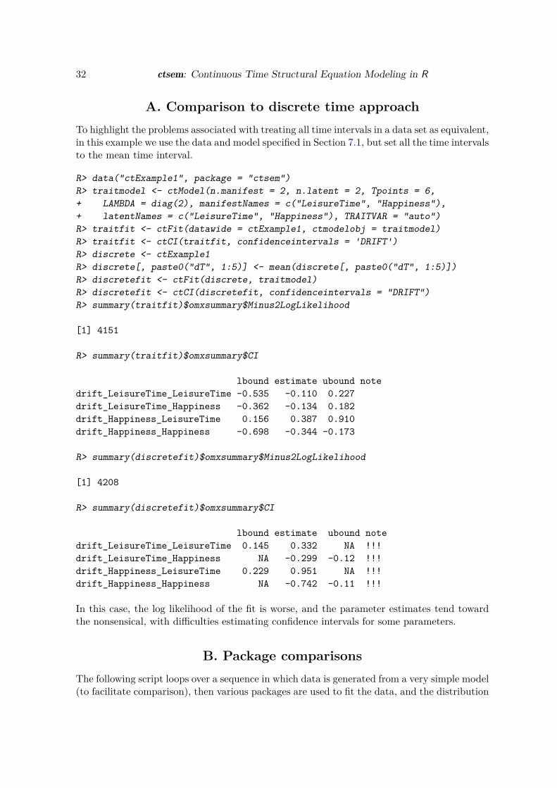
32 ctsem: Continuous Time Structural Equation Modeling in R
A. Comparison to discrete time approachTo highlight the problems associated with treating all time intervals in a data set as equivalent,in this example we use the data and model specified in Section 7.1, but set all the time intervalsto the mean time interval.
R> data("ctExample1", package = "ctsem")R> traitmodel <- ctModel(n.manifest = 2, n.latent = 2, Tpoints = 6,+ LAMBDA = diag(2), manifestNames = c("LeisureTime", "Happiness"),+ latentNames = c("LeisureTime", "Happiness"), TRAITVAR = "auto")R> traitfit <- ctFit(datawide = ctExample1, ctmodelobj = traitmodel)R> traitfit <- ctCI(traitfit, confidenceintervals = 'DRIFT')R> discrete <- ctExample1R> discrete[, paste0("dT", 1:5)] <- mean(discrete[, paste0("dT", 1:5)])R> discretefit <- ctFit(discrete, traitmodel)R> discretefit <- ctCI(discretefit, confidenceintervals = "DRIFT")R> summary(traitfit)$omxsummary$Minus2LogLikelihood
[1] 4151
R> summary(traitfit)$omxsummary$CI
lbound estimate ubound notedrift_LeisureTime_LeisureTime -0.535 -0.110 0.227drift_LeisureTime_Happiness -0.362 -0.134 0.182drift_Happiness_LeisureTime 0.156 0.387 0.910drift_Happiness_Happiness -0.698 -0.344 -0.173
R> summary(discretefit)$omxsummary$Minus2LogLikelihood
[1] 4208
R> summary(discretefit)$omxsummary$CI
lbound estimate ubound notedrift_LeisureTime_LeisureTime 0.145 0.332 NA !!!drift_LeisureTime_Happiness NA -0.299 -0.12 !!!drift_Happiness_LeisureTime 0.229 0.951 NA !!!drift_Happiness_Happiness NA -0.742 -0.11 !!!
In this case, the log likelihood of the fit is worse, and the parameter estimates tend towardthe nonsensical, with difficulties estimating confidence intervals for some parameters.
B. Package comparisonsThe following script loops over a sequence in which data is generated from a very simple model(to facilitate comparison), then various packages are used to fit the data, and the distribution

Journal of Statistical Software 33
−0.40 −0.35 −0.30 −0.25 −0.20 −0.15 −0.10
02
46
8
Density of estimates of drift parameter (true value −0.3)
N = 100 Bandwidth = 0.01359
Den
sity
ctsemctsarimaOpenMx
Figure 6: Density of drift parameter estimates of 30 simulated datasets of a single process,stationary model with no measurement error, a true drift value of −0.3, and 500 observationsof a single individual.
of parameter estimates is then plotted. ctsem is used to generate 500 time points of data fora single individual, for a single perfectly measured, stationary process with a drift value of−0.3. The different packages at times use different transformations of the parameters, but forease of comparison these are transformed to the drift parameter in ctsem. This comparison isnot intended as a critique of any package, differences in intended use and estimation routinesmay result in the observed differences, and it is hoped the provided code may help others toexplore alternatives when necessary.
R> if (!requireNamespace("cts", quietly = TRUE)) + stop(paste("cts package needed for this function to work.",+ "Please install it."), call. = FALSE)+ R> if (!requireNamespace("yuima", quietly = TRUE)) + stop(paste("yuima package needed for this function to work.",+ "Please install it."), call. = FALSE)+ R> Tpoints <- 500R> output <- matrix(NA, 100, 6)R> colnames(output) <- c('True', 'ctsem', 'cts', 'yuima', 'arima', 'OpenMx')R> for (i in 1:nrow(output)) + generatingModel <- ctModel(n.latent = 1, n.manifest = 1,+ Tpoints = Tpoints, LAMBDA = diag(1), DRIFT = matrix(-0.3, nrow = 1),

34 ctsem: Continuous Time Structural Equation Modeling in R
+ CINT = matrix(3, 1, 1), MANIFESTVAR = diag(0.00001, 1),+ DIFFUSION = t(chol(diag(5, 1))))+ output[i, 1] <- generatingModel$DRIFT # true value++ ctsemData <- ctGenerate(generatingModel, n.subjects = 1, burnin = 30)+ longData <- ctWideToLong(ctsemData, Tpoints = 500, n.manifest = 1)+ longData <- ctDeintervalise(longData)++ ## ctsem package+ ctsemModel <- ctModel(n.latent = 1, n.manifest = 1, Tpoints = Tpoints,+ MANIFESTVAR = diag(0.00001, 1), LAMBDA = diag(1))++ ctsemFit <- ctFit(ctsemData, ctsemModel, stationary = "T0VAR")+ output[i, 2] <- mxEval(DRIFT, ctsemFit$mxobj)++ ## cts package+ ctsData <- longData[, c("time", "Y1")]+ library("cts")+ ctsFit <- car(ctsData, order = 1, scale = 1)+ output[i, 3] <- -1 * (1 + ctsFit$phi) / (1 - ctsFit$phi)++ ## yuima package (not plotted - potential issues due to dT = 1)+ library("yuima")+ mod <- setModel(drift = "drift * x + cint", diffusion = "diffusion")+ ou <- setYuima(model = mod, data = setData(longData[, "Y1"],+ delta = 1))+ mlout <- qmle(ou, start = list(drift = -0.3, diffusion = 1, cint = 1))+ output[i, 4] <- mlout@coef[2]++ ## arima (from stats package, discrete time analysis only)+ arfit <- arima(longData[, "Y1"], order = c(1, 0, 0))+ log(arfit$coef[1]) # transform ar1 parameter to drift parameter+ output[i, 5] <- log(arfit$coef[1])++ ## OpenMx state space function+ ctsemModel <- ctModel(n.latent = 1, n.manifest = 1, Tpoints = Tpoints,+ MANIFESTVAR = diag(0.0001, 1), T0VAR = diag(1), LAMBDA = diag(1))+ cdim <- list("Y1", "eta1")++ amat <- mxMatrix("Full", 1, 1, TRUE, 0.3, name = "A", lbound = -10)+ bmat <- mxMatrix("Full", 1, 1, FALSE, 0, name = "B")+ cmat <- mxMatrix("Full", 1, 1, FALSE, 1, name = "C", dimnames = cdim)+ dmat <- mxMatrix("Full", 1, 1, TRUE, 1, name = "D")+ qmat <- mxMatrix("Full", 1, 1, TRUE, 1, name = "Q")+ rmat <- mxMatrix("Diag", 1, 1, FALSE, 0.0001, name = "R")+ xmat <- mxMatrix("Full", 1, 1, TRUE, 7, name = "x0", lbound = -10,+ ubound = 10)

Journal of Statistical Software 35
+ pmat <- mxMatrix("Diag", 1, 1, FALSE, 1, name = "P0")+ umat <- mxMatrix("Full", 1, 1, FALSE, 1, name = "u")+ tmat <- mxMatrix("Full", 1, 1, name = "time", labels = "data.time")++ osc <- mxModel("AR1",+ amat, bmat, cmat, dmat, qmat, rmat, xmat, pmat, umat, tmat,+ mxExpectationStateSpace("A", "B", "C", "D", "Q", "R", "x0", "P0",+ "u"), mxFitFunctionML(), mxData(longData, "raw"))++ oscr <- mxRun(osc)++ output[i, 6] <- log(mxEval(A, oscr))+ # end for loopR> plot(density(output[1:i, 2]), xlim = c(-0.4, -0.1), lty = 2, lwd = 2,+ ylab = "Density",+ main = "Density of estimates of drift parameter (true value -0.3)")R> points(density(output[1:i, 3]), col = "red", type = "l", lty = 3,+ lwd = 3)R> points(density(output[1:i, 5]), col = "blue", type = "l", lwd = 2,+ lty = 2)R> points(density(output[1:i, 6]), col = "green", type = "l", lwd = 4,+ lty = 5)R> legend("topleft", bty = "n", text.col = c("black","red","blue",+ "green"), legend = c("ctsem", "cts", "arima", "OpenMx"))
Affiliation:Charles DriverCenter for Lifespan PsychologyMax Planck Institute for Human DevelopmentLentzeallee 9414195 Berlin, GermanyTelephone: +49 30 82406-367E-mail: [email protected]: http://www.mpib-berlin.mpg.de/en/staff/charles-driver
Journal of Statistical Software http://www.jstatsoft.org/published by the Foundation for Open Access Statistics http://www.foastat.org/
April 2017, Volume 77, Issue 5 Submitted: 2015-02-19doi:10.18637/jss.v077.i05 Accepted: 2015-12-07