continuous sensorimotor control mechanisms in … · continuous sensorimotor control mechanisms in...
TRANSCRIPT
CONTINUOUS SENSORIMOTOR CONTROL MECHANISMS IN POSTERIOR
PARIETAL CORTEX: FORWARD MODEL ENCODING AND TRAJECTORY
DECODING
Thesis by
Grant Haverstock Mulliken
In Partial Fulfillment of the Requirements for the
Degree of
Doctor of Philosophy
CALIFORNIA INSTITUTE OF TECHNOLOGY
Pasadena, California
2008
(Defended April 22, 2008)

ii
© 2008
Grant Haverstock Mulliken
All Rights Reserved

iii
Dedicated to:
My loving family:
THM, SKM and ASM
CBH and SBH

iv
ACKNOWLEDGEMENT
I am deeply thankful for the exceptional research opportunities that my advisor, Richard Andersen, has afforded me during my time at Caltech. In addition to the lure of the CNS program at Caltech, a major motivation to move to Pasadena stemmed from a chance to participate in Richard’s neural prosthetic project; to collaborate with a team of top engineers and scientists developing a “brain-machine interface” that will assist paralyzed patients. From day one, Richard gambled on me and allowed me to jump directly into the heart of the project, attempting an exciting experiment to read out the thoughts of a monkey and use them to control an external device — truly an engineer-turning-neuroscientist’s dream come true. Beyond giving me this tremendous opportunity, Richard demonstrated unwavering patience and understanding while mentoring me in my early scientific years. His wisdom and well-timed advice always pointed me down the most interesting and rewarding path, which admittedly was often not apparent to me at first glance. Richard’s gifted intuition and sharply-tuned thoughts were outshined only by his genuine compassion for me and other members of the laboratory, making for a warm and collegial intellectual environment in which I could thrive. I am truly blessed to have had the opportunity to work with and learn from a master of systems neuroscience. I would also like to thank my distinguished committee members: Joel Burdick, Christof Koch, Pietro Perona and Shinsuke Shimojo, world-class researchers whose enthusiasm reverberates throughout the CNS community. Joel was my co-advisor and I’m thankful to him for many helpful discussions on decoding and autonomous electrode control. I am grateful to Christof for many inspiring conversations we had at the gym, on the rock, etc. Pietro Perona graciously allowed me to rotate in his lab during my first year in CNS, introducing me to the joys and rigors of computer vision and machine learning. I am thankful to Shin for serving as my committee chair, providing invaluable advice these last few months. I have had the opportunity to work with many talented colleagues during my time at Caltech. First and foremost, I thank my collaborator Sam Musallam, who took me under his wing, allowed me to share his rig and introduced me to monkey physiology. Sam’s willingness to drop whatever he was doing and “climb” into the rig to debug or hand me the reins in the OR or entertain my crazy ideas were all pivotal to the successful completion of this thesis. I thank Rajan Bhattacharrya and EunJung Hwang, officemates and dear friends. Rajan was always ready to lend an attentive ear when I needed to discuss new half-cocked ideas or statistical analyses. Beyond being the first referee for many of my ideas, Rajan and I shared countless adventures in monkey physiology made all the more memorable by Gizmo and Chewie. A brilliant scientist with a gentle spirit, EunJung was always a pleasure to work with. Her expertise in computational motor control was invaluable when going over the latest version of a decoding algorithm or exploring the viability of my ideas regarding forward models in parietal cortex. I thank Bijan Pesaran, an expert neurophysiologist who imparted many valuable lessons to me. Bijan’s unique ability to quickly dichotomize my ideas, sifting out the fat, helped me refine my argumentation and ultimately made me into a more mature scientist. Bijan’s compassion and encouragement when things temporarily went south was invaluable — I
v
am grateful for his friendship. Zoltan Nadasdy and Brian Lee were two other brilliant colleagues who shared the rig next door to mine, as well as hotel rooms at SFN. Zoltan’s quick wit and Brian’s uncanny ability to give and receive jokes made the hours pass by quickly. Thanks to Marina Brozovic for countless bits of advice during my first three years (on a variety of topics). I thank Mike Campos, one year my senior in the CNS program, and a friend and advisor for all 6 years. Thanks to friend Alex Gail, a scientist of exemplary character, for his dependable electrophysiology advice. I recently had the tremendous opportunity to collaborate with Markus Hauschild, a gifted engineer-turning-neuroscientist with whom I share a lot in common (including a fondness for Ernie’s tacos). I am thankful for the stimulating discussions we’ve had about decoding and coordinate frame representations in PPC. I also thank Eddie Branchaud and Mike Wolf of the Burdick Lab for many exciting adventures while pioneering autonomous control of 6 electrodes using the NAN microdrive! I am indebted to the superb staff of the Andersen Lab — without any of whom this thesis work would not have been possible. They were all a joy to work with and include Kelsie Pejsa, Nicole Sammons, Viktor Shcherbatyuk and Tessa Yao. Kelsie and Nicole — thank you for training me in numerous procedures and putting up with my comic relief (or lack thereof) in the OR. Viktor — thank you for all of your fast-acting and reliable expertise. Without fail, you were always in the house! Thanks to Tessa for your friendship, bowls of chocolate, and ALL of your help. Many other friends have made my time at Caltech truly special: Alex Holub for his camaraderie on and off the job and sharing three joint-birthday parties; Asha Iyer for her many wonderful gestures including bringing me cold medicine; Vivek Jayaraman for encouraging me to come to Caltech; my Catalina roommates Joey Genereux and Jeff Fingler for living with me, and my CNS class members: Allan Drummond for his Golom impression, Alan Hampton for late-night mountain bike rides, Kai Shen for riding the bull, and David Soloveichik for his blend of brilliance and humility. There are many others I would like to acknowledge, so with regret I’ll only briefly mention colleagues that I was fortunate to interact with during my PhD: Igor Kagan, He Cui, Hilary Glidden, Elizabeth Torres, Brian Corneil, Boris Breznen, and Daniel Rizzuto. Finally, I would like to thank my family. My parents, Steve and Taffy, have made innumerable sacrifices that have given me unearned opportunities to achieve my goals. The examples they set in their own careers: their competitive spirits, hunger for lifelong learning, and unselfish compassion for others are living lessons that I cherish. I want to thank my sister, Abby, for her ever-present support and willingness to be a brother’s best buddy from the early years and onward. To my grandfather, Charles, thank you for encouraging me at an early age to understand the mysteries of the natural world, instilling in me a curiosity to understand the way things work. And to my grandmother, Susan, thank you for the countless hours of hearts and cribbage that no doubt sharpened my thinking, having played with the best. And to my dearest Mary, thank you for caring for me, for enduring my neurosis, for patiently waiting months in Boston while I finish up this thesis, and most of all for guiding me on a path that is most joyful to travel.

vi
ABSTRACT
During goal-directed movements, primates are able to rapidly and accurately control a
movement despite substantial delay times (more than 200 milliseconds) incurred in the
sensorimotor control loop. To compensate for these large delays, it has been proposed
that the brain uses an internal forward model of the arm to estimate current and upcoming
states of a movement, which would be more useful for rapid online control. To study
online control mechanisms in the posterior parietal cortex (PPC), we recorded from
single neurons while monkeys performed a joystick task. Neurons encoded the static
target direction and the dynamic heading direction of the cursor. The temporal encoding
properties of many heading neurons reflected a forward estimate of the current state of
the cursor that is neither directly available from passive sensory feedback nor compatible
with outgoing motor commands, and is thus consistent with PPC serving as a forward
model for online sensorimotor control. In addition, we found that the space-time tuning
functions of these neurons mostly encode straight and approximately instantaneous
trajectories.
Recent advances in cortical prosthetics have focused on recording neural activity in
motor cortices and decoding these signals to control the trajectory of a cursor on a
computer screen. Building on our encoding results, we demonstrate that joystick-
controlled trajectories can also be decoded from PPC ensembles, presumably extracting
the dynamic state of the cursor from a forward model. Remarkably, we found that we

vii
could accurately reconstruct a monkey’s trajectories using only 5 simultaneously
recorded PPC neurons. Furthermore, we tested whether we could decode trajectories
during closed-loop brain control sessions, in which the real-time position of the cursor
was determined solely by a monkey’s thoughts. The monkey learned to perform brain
control trajectories at 80% success rate (for 8 targets) after just 4–5 sessions. This
improvement in behavioral performance was accompanied by a corresponding
enhancement in neural tuning properties (i.e.,, increased tuning depth and coverage of 2D
space) as well as an increase in offline decoding performance of the PPC ensemble. This
work marks an important step forward in the development of a neural prosthesis using
signals from PPC.

viii
TABLE OF CONTENTS
Acknowledgement………………….........……………………...…...…………..…
Abstract ………………………………………..………………………………..….
Table of Contents ……………………………………………..………………..…..
List of Illustrations ……………………………………………………..……..……
Chapter 1: Introduction ………………………………………………..………..….
1.1 Internal models for sensorimotor integration …...………………………………..
1.2 Encoding of intention and anticipation in PPC: the seat of the forward model? ...
1.3 Forward state estimation to compensate for sensory delay times ……………......
1.3.1 A forward model can be used to cancel sensory reafference …………………..….
1.4 Continuous sensorimotor control and state estimation in PPC …………...……...
1.5 A PPC neural prosthesis: continuous closed-loop control of an end effector …....
Chapter 2: Forward Estimation of Movement State in Posterior Parietal Cortex ...
2.1 Summary ……………..……………….……………………………………....….
2.2 Introduction …………………………...….………...…………………………….
2.3 Results …………………………………......………….………………………….
2.3.1 Space-time tuning …………………………..………………………………….….
2.3.2 Static encoding of goal angle …………………..…………….…………...…….....
2.3.3 Temporal encoding of movement angle …………..…...……..…………………....
2.3.4 Dynamic tuning and separability of movement angle STTF ….………..…...….....
2.4 Discussion …………………...…………………………………………..…….....
2.5 Methods ………………….……………...……………………………...………...
iv
vi
viii
xi
1
2
2
8
12
13
19
28
28
29
33
33
37
38
42
46
51
ix
2.5.1 Behavioral task ………………….…….…………………….……………………..
2.5.2 Space-time tuning analysis …………………….……………………………..…....
2.5.3 Information theoretic analysis …………….………….……………………….…...
2.5.4 Temporal dynamics and curvature of movement angle STTF ……...……….....….
2.5.5 Separability of movement angle STTF ………………………………..………......
2.6 Supporting information …………...……………………………………………...
2.6.1 Residual tuning significance testing ………………………………………...…….
2.6.2 Peak mutual information as a function of optimal lag time …………….………....
2.6.3 Neural stationarity …………………………………………….…..……….………
2.6.4 Optimal lag time statistical analysis …………………….……………….……..….
2.6.5 Velocity space-time tuning analysis ………………………………………...…….
2.6.6 Mutual information as a function of elapsed time ………………….………...…...
Chapter 3: Decoding Trajectories from Posterior Parietal Cortex Ensembles …....
3.1 Summary …………………………………………...…………………………….
3.2 Introduction …………………………………………...………………………….
3.3 Materials and methods …………………………………………...………...…….
3.3.1 Animal preparation ……………………………………………………….……….
3.3.2 Neurophysiological recording ………….…………………….………..……...…...
3.3.3 Experimental design …………………….………………….…..……………….....
3.3.4 Offline algorithm construction ………….……….………………………..…….....
3.3.5 Ridge regression ………………………….…….…………..………………...……
3.3.6 Goal-based Kalman filter ……………………………………………………….....
3.3.7 Model assessment …………………………………………...………………...…..
3.3.8 Neural unit waveform analysis ………………………………………...……...…..
3.4 Results ………...………………………………………………………………….
3.4.1 Offline decoding ………………………………………...………………..……….
3.4.2 Position decoding performance: model comparisons ……………………….….....
3.4.3 AMEA vs. FMEA decoding performance ………………….……...…..……….....
3.4.4 Reconstruction of behavioral and task parameters ……………….…………...…..
3.4.5 Lag time analysis …………………………...……………………………………..
3.5 Discussion …………………….………………………………...………………...
3.5.1 Considerations for decoding trajectories from PPC ……………..………..….…….
51
52
56
58
59
62
63
65
66
68
72
73
80
80
81
82
82
83
84
86
87
90
94
95
95
95
96
100
102
104
107
107

x
3.5.2 Decoding efficiency: AMEA vs. FMEA ………………….…………….…………
3.6 Supplemental material …………………...………………………………….....…
3.6.1 Ridge shrinkage and the effective degrees of freedom ….….……………………..
3.6.2 Discrete G-Kalman filter two-step estimation ………………...……………..........
3.6.3 Discrete G-Kalman filter stability …………………………….…...……….......….
Chapter 4: Using PPC to Continuously Control a Neural Prosthetic ………......…
4.1 Summary ……………………...………………………………………………….
4.2 Introduction ……………………...…………………………………………….....
4.3 Materials and methods ……………………………...………………………...….
4.3.1 Animal preparation ………………………...……….………………………..……
4.3.2 Neurophysiological recording ………………………..……………........................
4.3.3. Experimental design …………………………………..………...…...………...….
4.3.4 Closed-loop brain control analysis ……………………..………...…………..……
4.4 Results ………………………...………………………………………………….
4.4.1 Behavioral performance ………….…………………………………..………...….
4.4.2 Brain control learning effects …….…………………………………..............……
4.5 Discussion ……………………………………………………...………………...
4.5.1 Learning to control a cursor using continuous visual feedback ….…….……….....
Chapter 5: Concluding Remarks ………………………………………….....……
5.1 Encoding properties of PPC neurons during online control of movement …...….
5.1.1 Summary of significant findings ………………………….………………….…....
5.1.2 Directions for further investigation ……………………….……………………….
5.2 Trajectory decoding and a PPC neural prosthetic ……………...………………...
5.2.1 Summary of significant findings …………………………….…………………….
5.2.2 Directions for further investigation ………………………….………………….…
109
111
111
112
114
119
119
120
122
122
123
123
124
125
125
130
136
136
140
140
140
141
143
143
143
xi
LIST OF ILLUSTRATIONS
Figure 1-1 ……………………..……………….…………..………….……………
Figure 1-2 ………………………..………………………..….………………….…
Figure 1-3 ……………..……………..………………………..…………………....
Figure 1-4 ……………….……………………….....................................................
Figure 2-1 ………………………………..…………………………..…………..…
Figure 2-2 …………………………………..………….………………..……….....
Figure 2-3 …………………………………..………………………………..…..…
Figure 2-4 …………………………………..….………………………………...…
Figure S2-1 ……………..………………………..…………………………………
Figure S2-2 ………………..……………………..…………………………………
Figure S2-3 …………………..…………………..…………………………………
Figure S2-4 ……………………..………………..…………………………………
Figure S2-5 ………………………..……………..…………………………………
Figure S2-6 .…………………………..…………..……………………………...…
Figure 3-1 ….……………………………..………..…………………………….…
Figure 3-2 ………….………………………..……..…………………………….…
Figure 3-3 ………….…………………………..…..…………………………….…
Figure 3-4 …………………………………………....…………………………..…
Figure 3-5 ………………………………………..……..…………………………..
Figure 3-6 ………………………………………………….………………………. 106
4
12
15
22
30
35
40
44
62
65
66
70
74
76
85
97
99
101
104

xii
Figure S3-1 ……………………………..……………………..……………............
Figure 4-1 ………………………………..….……………………...........................
Figure 4-2 ………………………………...……………….......................................
Figure 4-3 …………………………………..…….……………...............................
Figure 4-4 …………………………………..….………….......................................
115
122
127
129
132

1
Chapter 1
INTRODUCTION
This world is but a canvas to our imaginations.
Henry David Thoreau
We continuously integrate and evaluate information sensed in our environment in order
to guide our decisions and actions with an aim to maximize our likelihood of survival.
Thriving in one’s environment therefore relies upon the ability of neural circuitry to
accurately specify an internal representation of the interaction of oneself and the outside
world. For example, the ability to carry out goal-directed activities such as building a
campfire, catching a fish or watercolor painting depend on the operation of a neural
model that links our sensory experience of the world with our body’s ability to act
competently within it. From a systems neuroscience perspective: where in the brain are
such internal models of sensorimotor experience located, how are they encoded, and can
they be measured directly? Second, from both a medical and engineering standpoint: can
we measure such cognitive signals directly and harness them to causally control an
external apparatus other than our own limbs?

2
1.1 Internal models for sensorimotor integration
A growing body of clinical and psychophysical evidence supports the theory that the
brain makes use of an internal model during control of movement; a sensorimotor
representation of the interaction of one’s self with the physical world (M. Kawato et al.,
1987; M. I. Jordan, 1995). Two primary types of internal models for sensorimotor control
have been proposed: the forward model and the inverse model. A forward model predicts
the sensory consequences of a movement (M. I. Jordan and D. E. Rumelhart, 1992; D. M.
Wolpert et al., 1995). That is, it mimics the behavior of a motor system by predicting the
expected, upcoming state of an end effector (e.g. one’s own limb) as a function of the
characteristic dynamics of the system as well as stored copies of recently issued motor
commands. Conversely, an inverse model encodes the motor commands necessary to
produce a desired outcome (C. G. Atkeson, 1989). That is, an inverse model estimates the
set of procedures (e.g. motor commands) that will cause a particular state of the motor
system to occur. While inverse models likely play an important role in sensorimotor
control, they will not be discussed further in this thesis and instead emphasis will be
placed on the forward model, and in particular the role of the posterior parietal cortex
(PPC) in forward state estimation for motor planning and control.
1.2 Encoding of intention and anticipation in PPC: the seat of the forward model?
PPC is a critical node for bridging sensory and motor representations in the brain. PPC
associates multiple sensory modalities (e.g., visual - the dominant input to PPC,
somatosensory and auditory) and transforms these inputs into a representation useful for
guiding actions to objects in the external world (R. A. Andersen and C. A. Buneo, 2002).

3
Anatomically, PPC is positioned along the dorsal visual pathway of the brain, also known
as the vision-for-action pathway (L. G. Ungerleider and M. Mishkin, 1982; M. A.
Goodale, 1998). Evidence from lesions studies indicates that damage to PPC results in an
inability to link the sensory requirements of a task with the appropriate motor behavior
needed to complete it. For example, parietal lesion patients can have difficultly planning
skilled movements, a condition known as apraxia (N. Geshwind and A. R. Damasio,
1985). Impairments from apraxia can range from an inability to properly follow
instructions that describe how to make a particular movement to how to coordinate a
sequence of movements to accomplish an end goal.

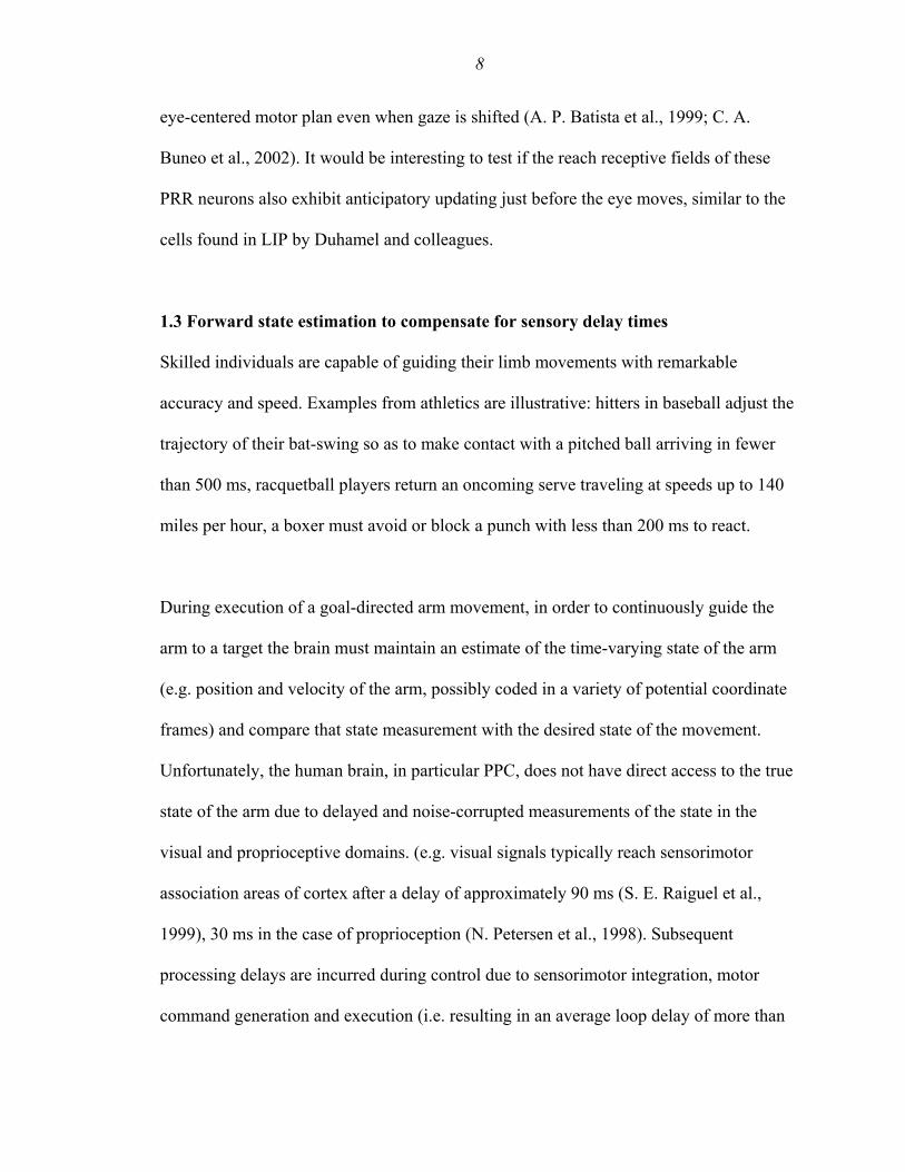
4
Figure 1-1. The two streams of visual information in the primate brain and reach intention areas of
PPC. (A) The dorsal stream processes visual information for movement and is concerned with how
visual information is used to form an action. The “vision for action” pathway branches from the
occipital lobe to the posterior parietal cortex (PPC), which performs sensorimotor transformations, and
to the motor cortices, which are involved in issuing motor commands to the muscles. The ventral stream

5
is largely concerned with visual perception, for example the inferotemporal cortex (IT) is critical for
discriminating and recognizing objects. This whole-brain view shows the surface location of the parietal
reach region (PRR) located along the medial bank of the intraparietal sulcus (IPS), which can extend to
depths of up to 10 mm. Moving anterior and slightly anterior, PRR merges into area 5, which is situated
more on the surface of cortex. (B) Coronal section designated by the dashed vertical line in panel (A),
illustrating the convoluted geometry of the IPS as well as the relative depths of PRR and area 5 (C)
Nissl-stained coronal section of the rhesus macaque brain, clearly showing the intraparietal sulcus.
Coronal section was obtained from www.brainmaps.org (S. Mikula et al., 2007).
Numerous neurophysiological studies in monkeys have shed light on the neural correlates
of reach planning in PPC. Monkeys have served as a successful model for studying
sensorimotor representations in humans since the two species engage in a variety of
similar sensorimotor behaviors. Moreover, functional magnetic resonance imaging
(fMRI) studies have provided evidence that PPC’s functional role is similar in both
monkeys and humans (J. F. X. DeSouza et al., 2000; M. F. S. Rushworth et al., 2001; J.
D. Connolly et al., 2003). When trained monkeys plan a reach to an illuminated target,
the firing rates of neurons in the medial bank of the intraparietal sulcus (MIP) generally
reflect a combination of both sensory and motor parameters (V. B. Mountcastle et al.,
1975; D. L. Robinson et al., 1978; R. A. Andersen and C. A. Buneo, 2002). Importantly
however, during a memory period in which the monkey must maintain a reach plan to the
remembered location of an extinguished target, elevated neural activity persists in PPC
before the reach is executed, suggesting that these neurons likely encode the intention to
reach, rather than the visual stimulus location (L. H. Snyder et al., 1997). Furthermore,
neurons in MIP are generally correlated more strongly with the motor goal, and not the
visual cue, during anti-reach paradigms in which the target cue direction is dissociated

6
from the reach direction (J. F. Kalaska and D. J. Crammond, 1995; E. N. Eskandar and J.
A. Assad, 1999; A. Gail and R. A. Andersen, 2006). Based on these planning studies, it is
tempting to hypothesize that memory-period activity might also reflect a prediction of the
sensory consequences of an upcoming arm movement (i.e. the expected endpoint of a
reach) derived from efference copy, a signal that is compatible with the output of a
forward model of arm position. More generally, one could interpret the effector-specific
segregation of planning activity in the intraparietal sulcus, such as MIP responses
associated with a reach and LIP responses involved in the formulation of a saccade (R. A.
Andersen and C. A. Buneo, 2002), as a prediction of the future state of an effector, the
motor command itself or both. Along these lines multiple researchers have also suggested
that the ‘early’ discharge of neurons in area 5 prior to initiation of an arm movement
might reflect an efference copy signal fed back to PPC from frontal motor areas (J. Seal
et al., 1982; J. F. Kalaska et al., 1983). Interestingly, Seal and colleagues also showed
that area 5 responses that occurred prior to movement onset were generally not sensory in
origin and furthermore demonstrated that these early responses persisted even after
deafferentation. However, caution should be advised when attempting to infer the causal
flow of information in the parieto-frontal circuit during reach preparation using single-
area correlation analyses. Furthermore, it is quite possible that planning and forward
model prediction may be carried out by distinct neural processes within the PPC. Future
simultaneous multi-area recordings, combined with micro-stimulation approaches, should
shed light on the directional flow of information in these recurrent inter-area circuits
during movement preparation.

7
PPC is also a good candidate for a forward model of eye position since a variety of eye
behavior related signals, such as saccade and fixation responses have been described in
this region (V. B. Mountcastle et al., 1975). Whereas area 7a saccade responses begin
largely after the saccade, area LIP saccade responses tend to occur before, during or after
saccades (R. A. Andersen et al., 1987). Interestingly, Duhamel and colleagues also
showed that the receptive fields of neurons in LIP can update their receptive fields before
an eye movement occurs (J. R. Duhamel et al., 1992). 44% (16 out of 36) of their LIP
sample anticipated the sensory effects of an impending saccade (i.e. a stimulus appearing
in the future location of the receptive field), and adjusted their responses approximately
80 milliseconds (ms) before the saccade was launched. It is conceivable that this
predictive remapping relies upon a forward model of eye position within PPC, which
estimates the upcoming eye position from oculomotor commands, though direct evidence
of the anticipatory eye position signal itself in PPC has not been reported. Fixation
related activity commonly found in PPC is sensitive for eye position, and this response
characteristic is often multiplicatively combined with the sensory and saccade-related
activity of single neurons (R. A. Andersen et al., 1987). An eye position signal in PPC
could be derived from proprioceptive feedback from the eye muscles (X. L. Wang et al.,
2007) and/or the integration of saccade command signals. It would be interesting to see if
a component of the eye position signal might also provide anticipatory information
(ahead of passive sensory feedback) about the current state of the eye position during
fixations between saccades. Last, Batista and colleagues showed that neurons in PRR,
which predominantly encode an intended reach direction in eye-centered coordinates,
update their receptive fields when an intervening saccade occurs, thereby maintaining an
8
eye-centered motor plan even when gaze is shifted (A. P. Batista et al., 1999; C. A.
Buneo et al., 2002). It would be interesting to test if the reach receptive fields of these
PRR neurons also exhibit anticipatory updating just before the eye moves, similar to the
cells found in LIP by Duhamel and colleagues.
1.3 Forward state estimation to compensate for sensory delay times
Skilled individuals are capable of guiding their limb movements with remarkable
accuracy and speed. Examples from athletics are illustrative: hitters in baseball adjust the
trajectory of their bat-swing so as to make contact with a pitched ball arriving in fewer
than 500 ms, racquetball players return an oncoming serve traveling at speeds up to 140
miles per hour, a boxer must avoid or block a punch with less than 200 ms to react.
During execution of a goal-directed arm movement, in order to continuously guide the
arm to a target the brain must maintain an estimate of the time-varying state of the arm
(e.g. position and velocity of the arm, possibly coded in a variety of potential coordinate
frames) and compare that state measurement with the desired state of the movement.
Unfortunately, the human brain, in particular PPC, does not have direct access to the true
state of the arm due to delayed and noise-corrupted measurements of the state in the
visual and proprioceptive domains. (e.g. visual signals typically reach sensorimotor
association areas of cortex after a delay of approximately 90 ms (S. E. Raiguel et al.,
1999), 30 ms in the case of proprioception (N. Petersen et al., 1998). Subsequent
processing delays are incurred during control due to sensorimotor integration, motor
command generation and execution (i.e. resulting in an average loop delay of more than

9
100 ms for proprioceptive control (M. Flanders and P. J. Cordo, 1989) and over 200 ms
for visuomotor control (A. P. Georgopoulos et al., 1981; R. C. Miall et al., 1993). These
long delay times severely limit a feedback control system’s ability to make rapid
adjustments to an ongoing movement and thus increase the likelihood that a reach
trajectory might become erroneous and/or unstable.
Remarkably, despite substantial transmission and processing delays in the sensorimotor
control loop, we are able to rapidly and accurately control our movement trajectories.
Therefore, passive sensory feedback must not be the only signal used by the brain to
estimate the current state of the arm. Fortunately the brain can also monitor recently
issued motor commands (i.e. efference copy), which could be transmitted centrally (e.g.
from frontal motor areas) with little delay time (e.g. one synapse + transmission time <
10 ms) and used by a forward dynamics model to form an estimate of the current or
upcoming state of the arm. (M. I. Jordan and D. E. Rumelhart, 1992; D. M. Wolpert et
al., 1995). Thus a forward model’s prediction can be made available immediately to
sensorimotor control structures in the brain, well in advance of late-arriving sensory
information. Since the output of the forward dynamics model reflects a best guess as to
what the next state of the arm will be, errors due to various sources of noise will
inevitably accumulate over time into this estimate. Therefore it is likely that sensory
observations, which arrive at later times, are also continually integrated by the brain in
order to update and refine the estimate of the forward dynamics model (R. C. Miall and
D. M. Wolpert, 1996). A system that estimates the state of a movement by combining the
output of a forward dynamics model with sensory feedback about the state is generally

10
referred to as an “observer” (G. C. Goodwin and K. S. Sin, 1984). For linear systems in
which the noise is additive and Gaussian, the optimal (i.e. in the mean squared error
sense) observer is a Kalman filter (R. E. Kalman, 1960). Wolpert and colleagues first
applied the Kalman filter to model how subjects estimate the sensorimotor state of the
hand during goal-directed reaches. They showed that a Kalman filter could accurately
account for subjects’ estimates of the perceived end location of their hand while making
arm movements in the dark (D. M. Wolpert et al., 1995). Therefore, the Kalman filter
serves as a useful theoretical model for studying sensorimotor state estimation in the
brain.
Two linear stochastic equations govern the basic operation of the Kalman filter:
111 −−− ++= kkkkk wBuxAx , (forward dynamics model) (1)
kkkk xHy ν+= , (state observation model) (2)
where xk is the time-varying state of the arm at time step k modeled as a linear function of
the previous state, xk-1 and the control term, uk. The control term is considered to be a
known motor command, which is likely specified by frontal motor areas (e.g. primary
motor cortex (M1)) and then fed back to sensorimotor circuits that perform state
estimation. For instance, the motor command at each time step might be determined
using an optimization procedure that minimizes a cost function associated with carrying
out a particular trajectory (E. Todorov, 2006). yk is a sensory measurement (visual and
proprioceptive) made at time step k (note that sensory feedback is actually a delayed
representation of the state of the arm).

11
In order to estimate the state of the arm at each time step k, the output of the forward
dynamics model, (i.e. a priori estimate), is linearly combined with the difference
between the output of the observation model (i.e. predicted sensory measurement) and the
actual sensory measurement. This, discrepancy, the ‘sensory innovation’, is then
optimally scaled by the Kalman gain, Kk, to produce an a posterior estimate of the state
of the arm,
−kx̂
( ) ˆˆˆ −− −+= kkkkk xHyKxx . (3)
In brief, discrete state estimation consists of a two-step recursive procedure; such that the
forward dynamics model generates an a priori estimate of the state, which is next refined
by potentially innovative information gleaned from the sensory input to form the final, a
posterior estimate. PPC, specifically the parietal reach region (PRR) and area 5, seems to
be a reasonable site for an observer to reside given its large number of feedback
connections from frontal areas (i.e. efference copy) and substantial sensory input from
both visual and somatosensory domains (E. G. Jones and T. P. Powell, 1970; P. B.
Johnson et al., 1996).

12
Figure 1-2. Flow diagram illustrating sensorimotor integration for reach planning and online control
(after M. Desmurget and S. Grafton, 2000). Items in rounded boxes denote pertinent sensorimotor
variables; computational processes are contained in rectangular boxes. Prior to a reach, an intended
trajectory is formulated as a function of both the initial state of the arm and the desired endpoint, the
target location. An inverse model is used to determine a set of motor plans that will result in the desired
trajectory. Motor plans are then issued (likely by the primary motor cortex, M1) and subsequently
executed by muscles acting within the physical environment (i.e. biomechanical plant hexagon).
Following movement onset, the path of the arm is continuously monitored and corrected, if necessary, to
ensure successful completion of the reach. Critical to rapid online correction of movement is the forward
model, which generates a rapid a priori estimate of the next state of the arm, , as a function of the
previous state and efference copy. Intermittent sensory feedback is used to refine the a priori estimate of
the forward dynamics model (observer output). This a posterior current state estimate, , is then
evaluated by comparing it with the target location in order to make corrections to subsequent motor
commands.
−kx̂
kx̂

13
1.3.1 A forward model can be used to cancel sensory reafference
A forward model’s ability to predict the sensory consequences of an action is also useful
to an organism because a given sensory outcome can be produced by a variety of possible
causes (R. W. Sperry, 1950; Weiskran.L et al., 1971; G. Claxton, 1975; J. F. A. Poulet
and B. Hedwig, 2003; K. E. Cullen, 2004; J. E. Roy and K. E. Cullen, 2004). In
particular, a forward model can provide an internal reference signal that is useful for
canceling the sensory effects of self-motion. For example, motion on our retina can occur
because of movement in the physical world (i.e., afference) or because of motion induced
by an eye movement itself (reafference). Therefore, in order to correctly perceive the
motion of an external stimulus, the brain must distinguish afferent motion from reafferent
motion. A subtractive comparison between a forward model’s estimate of the expected
sensory outcome of an eye movement and the actual sensory signals could remove this
retinal shift from our perception (T. Haarmeier et al., 2001). Reafference-canceling
mechanisms are likely to be in operation for perception of limb movements as well. A
forward model of the arm could be critical for distinguishing self-generated arm
movement from both movement of the environment and movement of one’s arm by an
external force.
1.4 Continuous sensorimotor control and state estimation in PPC
Clinical and psychophysical studies in humans have established that PPC is involved not
only in specifying movement plans, but also in the execution and control of ongoing
movement. For example, it is well known that lesions in parietal cortex often lead to optic
ataxia, impairment in locating and reaching to stimuli in 3D space (R. Balint, 1909; P.

14
Rondot et al., 1977; M. T. Perenin and A. Vighetto, 1988). For instance, optic ataxia
patients have difficulty making rapid and ‘automatic’ corrective movements when
guiding the hand to targets that have been jumped (L. Pisella et al., 2000). Similarly, Grea
and colleagues reported a patient with bi-lateral parietal lesions that was unable to amend
her movement to pick up a cylinder after it had been jumped to a new location at
movement onset (H. Grea et al., 2002). Interestingly, instead of making corrective
movements during the initial trajectory, the subject needed to perform two distinct
movements, one that represented the initial plan and a second movement to reach to the
new location of the cylinder. Using transcranial magnetic stimulation (TMS) applied to
the posterior parietal cortex, Desmurget and colleagues were able to transiently disrupt
the ability of most subjects to correct reaching trajectories made to targets that were
displaced around the time of movement onset (M. Desmurget et al., 1999). Later, Della-
Maggiore and colleagues showed that TMS applied to PPC interfered with the ability of
subjects to adapt to novel force-field environments (V. Della-Maggiore et al., 2004). An
intriguing, potentially unifying explanation for all of these deficits, which was originally
suggested by Wolpert and colleagues, is that PPC may serve as an observer, which forms
an internal estimate of the state of the arm during movement (D. M. Wolpert et al.,
1998a). A failure to accurately maintain this estimate online could result in an inability to
monitor and therefore correct an ongoing movement. Interestingly, Wolpert and
colleagues reported a parietal lesion patient who was unable to maintain an internal
estimate of the state of her hand. For example, she could not maintain a constant
precision grip force in absence of vision, without vision of her stationary arm she
perceived it to drift slowly in space over 10-20 seconds until eventually reporting it to

15
disappear, and finally when asked to make slow-pointing movements to peripheral targets
while maintaining central fixation, large errors accumulated in her trajectories (although
self-paced movements were not impaired).
Figure 1-3. Examples of patients with sensorimotor deficits due to parietal injury. (A) A patient with a
biparietal tumor is unable to guide his reach in order to successfully grasp a pen, although his ability to

16
see it was not impaired (D. G. Cogan, 1965). (B) Patient with Balint’s syndrome presents optic ataxia
symptoms, such that he is unable to direct an arm movement toward a visually cued target (i.e., pour
liquid into a glass) (R. S. Allison et al., 1969). (C) A patient with a left parietal lesion is unable to
properly orient his hand to successfully position it inside the slot (M. T. Perenin and A. Vighetto, 1988).
Evidence that PPC is involved in sensorimotor state estimation also comes from studies
of the mental simulation of movement, which presumably activates circuits overlapping
with those engaged during motor control, but while inhibiting execution of a movement
itself (K. M. Stephan et al., 1995; J. Decety, 1996; E. Gerardin et al., 2000). When
normal healthy subjects imagine making a goal-directed movement, mental simulation
time typically matches the time needed to execute that same movement (F. C. Donders,
1969; J. Decety and F. Michel, 1989). This suggests that the brain is able to maintain a
realistic estimate of the state of the hand over time while imagining a movement, despite
sensory feedback being unavailable. Interpreting this finding in the context of observer
theory, this capability suggests that the brain/observer is able to rely entirely upon the
output of a forward model to estimate the state of the arm during mental simulation (e.g.
Kalman gain in Equation 3 is set to zero) (R. Shadmehr and J. W. Krakauer, 2008).
Interestingly, patients with unilateral motor cortex lesions (A. Sirigu et al., 1995) who
show prolonged movement times compared to normal control subjects are still able to
accurately imagine the duration of their movements (i.e. the simulation time and
execution time remain well-matched for these patients). For example, aberrant motor
commands (u in Equation 1) that are produced by the motor cortex could theoretically be
used by an intact observer to predict the correct temporal sequence of hand states (and
therefore the trajectory duration) even for an impaired movement. Interestingly, patients

17
with lesions of the cerebellum (F. A. Kagerer et al., 1998) and of the basal ganglia (P.
Dominey et al., 1995) also do not show a difference between simulation and execution
times.
While M1, the cerebellum and the basal ganglia do not appear to be critically involved in
the state estimation during simulated movements, PPC does appear to be essential for
maintaining an internal representation of the state of the hand that is necessary for
representing a consistent relationship between simulated and execution time. Sirigu and
colleagues later reported an impairment in the ability to simulate a movement in patients
with right PPC lesions: the time needed to mentally simulate a movement was
significantly different (generally less) than the time necessary to execute that same
movement (A. Sirigu et al., 1996). (Note, similar to motor cortex lesion patients, actual
execution time was also prolonged compared to control subjects). This inconsistency
suggests that the brain was unable to reliably estimate the state of the hand after damage
to PPC. This impairment could be explained by multiple possible failures of the observer
model: 1) an error in the forward dynamics model (i.e. faulty A or B matrices in Equation
1), 2) an error when incorporating sensory feedback into the a priori estimate of the
forward dynamics model (i.e. faulty H or K matrices in Equation 3) or 3) a combination
of 1 and 2. Based on known strong sensory input to PPC, it is probable that PPC is
involved in integrating sensory feedback into the state estimate. However, because visual
and proprioceptive input were held constant during the above mental simulation tasks
(e.g. eyes were closed, muscle activity was absent) it is not likely that erroneous state
estimation was due exclusively to faulty integration of sensory feedback. Interestingly,

18
most parietal lesion patients significantly underestimated the time it would take to
complete a movement when simulating it. Therefore, such a systematic decrease in
imagined movement duration is more likely to have arisen due to an erroneous a priori
estimate made by a forward dynamics model, whose transition matrices A and B govern
the speed at which the arm propagates through space (rather than a faulty observation
model which relates sensory input to the state of the arm using a time-independent
model). Therefore, these mental simulation results suggest that PPC is also involved in
propagating the state of the arm forward in time using a forward dynamics model
(Equation 1). Assuming PPC incorporates sensory information into the forward model
state estimate as well, then PPC would be best described as an observer, as suggested by
Wolpert and colleagues.
Psychophysical and clinical reports have pointed to both the parietal lobe and the
cerebellum as candidate neural substrates for a forward model (R. C. Miall et al., 1993;
D. M. Wolpert et al., 1998a; D. M. Wolpert et al., 1998b; S. J. Blakemore and A. Sirigu,
2003). Desmurget and colleagues suggested that PPC encodes a forward model of the
arm’s dynamics from which it may also compute an estimate of the motor error (i.e. the
difference between the target vector and the movement vector), which could then be
transformed into a corrective motor command by the cerebellum (M. Desmurget and S.
Grafton, 2000). While these insights suggest that PPC and the cerebellum may be
involved in forward model control, finding direct neural evidence of forward model state
estimation in the brain has proven difficult.

19
Previous encoding studies have shown that area 5 neurons are correlated with a variety of
movement and task-related parameters (most notably velocity and target position) during
reaching movements made with a manipulandum (J. Ashe and A. P. Georgopoulos, 1994;
B. B. Averbeck et al., 2005). However, these studies concluded that area 5 largely
encodes a sensory (i.e. proprioceptive) representation that slightly lags the state of the
movement (i.e. lag time = -30 ms). In Chapter 2 we further investigate the neural
representation of online directional control signals in PPC while monkeys perform
center-out and obstacle avoidance joystick tasks. We provide new evidence that neurons
in PPC compute an estimate of the current and upcoming states of the cursor (G. H.
Mulliken et al., 2008). This finding provides the first direct evidence of a state estimate
that is derived from a forward model and is a starting point for future studies designed to
rigorously reverse-engineer the computational mechanisms and circuits involved in
forward model control.
1.5 A PPC neural prosthesis: continuous closed-loop control of an end effector
It would be interesting to test if dynamic state estimates in PPC, presumably reflecting
the operation of an observer could be used to causally control an external device, besides
our own limbs. During recent years, several groups have leveraged findings from decades
of primate neurophysiology toward the development of an important medical application,
a neural prosthesis to assist paralyzed individuals. Paralysis affects millions of people in
the United States and can occur as a result of stroke and cervical spine injuries as well as
neurodegenerative disorders such as amyotrophic lateral sclerosis (Lou Gehrig’s
Disease). Tragically, paralyzed patients are not able to send motor commands to control

20
their muscles nor are they able to experience sensation from their limbs. Importantly
however, these individuals can still think about moving, and thus maintain the capacity to
plan and specify instructions for the control of movement. Therefore, a neural prosthesis
could directly read out the desired movement intentions of these patients from regions of
the brain not affected by injury or disease. Sensorimotor areas of cortex, particularly
those which are strongly innervated by visual feedback projections (e.g., PPC) represent
candidate regions that are potentially useful for driving a neural prosthesis since their
primary source of input, visual information, is typically uncompromised after paralysis
(Fig 1-4).
A cortical prosthesis is composed of multiple parts, which constitute a marriage of
engineering and scientific advances. Neural signals from a targeted brain region (i.e.,
spiking activity of neurons and the local field potential (LFP)) are extracted by measuring
the extracellular potential at many different sites in the cortical tissue using metal multi-
electrode arrays, which currently can record from on the order of 100 signals
simultaneously. Amplification and filtering of these neural signals occurs proximal to the
implant, maximizing the signal-to-noise ratio of each neural measurement. Signal-
processing, including spike-sorting, firing rate calculations and space-time analysis of
LFPs, is then performed before passing these assuaged signals along (e.g., via wireless
transmission) to a decoding algorithm. The decoding algorithm then computes an optimal
estimate of the desired movement outcome from the neural activity, which is then used to
control an external device.
21
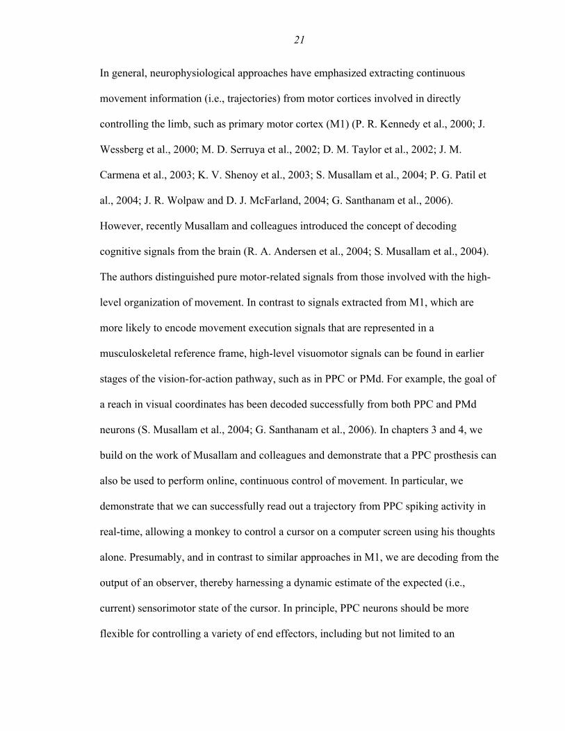
In general, neurophysiological approaches have emphasized extracting continuous
movement information (i.e., trajectories) from motor cortices involved in directly
controlling the limb, such as primary motor cortex (M1) (P. R. Kennedy et al., 2000; J.
Wessberg et al., 2000; M. D. Serruya et al., 2002; D. M. Taylor et al., 2002; J. M.
Carmena et al., 2003; K. V. Shenoy et al., 2003; S. Musallam et al., 2004; P. G. Patil et
al., 2004; J. R. Wolpaw and D. J. McFarland, 2004; G. Santhanam et al., 2006).
However, recently Musallam and colleagues introduced the concept of decoding
cognitive signals from the brain (R. A. Andersen et al., 2004; S. Musallam et al., 2004).
The authors distinguished pure motor-related signals from those involved with the high-
level organization of movement. In contrast to signals extracted from M1, which are
more likely to encode movement execution signals that are represented in a
musculoskeletal reference frame, high-level visuomotor signals can be found in earlier
stages of the vision-for-action pathway, such as in PPC or PMd. For example, the goal of
a reach in visual coordinates has been decoded successfully from both PPC and PMd
neurons (S. Musallam et al., 2004; G. Santhanam et al., 2006). In chapters 3 and 4, we
build on the work of Musallam and colleagues and demonstrate that a PPC prosthesis can
also be used to perform online, continuous control of movement. In particular, we
demonstrate that we can successfully read out a trajectory from PPC spiking activity in
real-time, allowing a monkey to control a cursor on a computer screen using his thoughts
alone. Presumably, and in contrast to similar approaches in M1, we are decoding from the
output of an observer, thereby harnessing a dynamic estimate of the expected (i.e.,
current) sensorimotor state of the cursor. In principle, PPC neurons should be more
flexible for controlling a variety of end effectors, including but not limited to an
22
antrhopomorphic arm. Furthermore, the richness of signals available in PPC may
ultimately be advantageous for inferring variables beyond just sensorimotor signals,
which may include, for example, the expected value of an impending action or one’s
behavioral or cognitive state (S. Musallam et al., 2004).
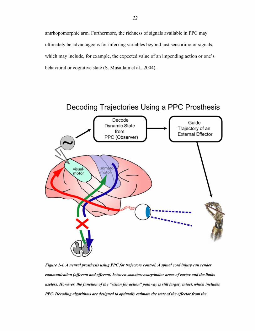
Figure 1-4. A neural prosthesis using PPC for trajectory control. A spinal cord injury can render
communication (afferent and efferent) between somatosensory/motor areas of cortex and the limbs
useless. However, the function of the “vision for action” pathway is still largely intact, which includes
PPC. Decoding algorithms are designed to optimally estimate the state of the effector from the

23
measurement of neural activity from PPC ensembles. In principle, the cognitive nature of signals in PPC
could be used to control a variety of end effectors, such as a robotic arm.
References
Allison RS, Hurwitz LJ, White JG, Wilmot TJ (1969) A follow-up study of a patient with Balint's syndrome. Neuropsychologia 7:319-333.
Andersen RA, Buneo CA (2002) Intentional maps in posterior parietal cortex. Ann Rev Neurosci 25:189-220.
Andersen RA, Essick GK, Siegel RM (1987) Neurons of area-7 activated by both visual-stimuli and oculomotor behavior. Exp Brain Res 67:316-322.
Andersen RA, Burdick JW, Musallam S, Pesaran B, Cham JG (2004) Cognitive neural prosthetics. Trends in Cognitive Sciences 8:486-493.
Ashe J, Georgopoulos AP (1994) Movement parameters and neural activity in motor cortex and area 5. Cereb Cortex 4:590-600.
Atkeson CG (1989) Learning Arm Kinematics and Dynamics. Annual Review of Neuroscience 12:157-183.
Averbeck BB, Chafee MV, Crowe DA, Georgopoulos AP (2005) Parietal representation of hand velocity in a copy task. J Neurophysiol 93:508-518.
Balint R (1909) Seelenlahmung des “Schauens,” optische Ataxie, raumliche Storung der Aufmerksamkeit. Monatsschr Psychiatr Neurol 25:51-81. Batista AP, Buneo CA, Snyder LH, Andersen RA (1999) Reach plans in eye-centered
coordinates. Science 285:257-260. Blakemore SJ, Sirigu A (2003) Action prediction in the cerebellum and in the parietal
lobe. Exp Brain Res 153:239-245. Buneo CA, Jarvis MR, Batista AP, Andersen RA (2002) Direct visuomotor
transformations for reaching. Nature 416:632-636. Carmena JM, Lebedev MA, Crist RE, O'Doherty JE, Santucci DM, Dimitrov DF, Patil
PG, Henriquez CS, Nicolelis MAL (2003) Learning to control a brain-machine interface for reaching and grasping by primates. PLOS Biology 1:193-208.
Claxton G (1975) Why can't we tickle ourselves? Percept Mot Skills 41:335-338. Cogan DG (1965) Opthalmic manifestations of bilateral non-occipital cerebral lesions. Br
J Opthalmol 49:281-297. Connolly JD, Andersen RA, Goodale MA (2003) FMRI evidence for a 'parietal reach
region' in the human brain. Experimental Brain Research 153:140-145. Cullen KE (2004) Sensory signals during active versus passive movement. Current
Opinion in Neurobiology 14:698-706. Decety J (1996) Do imagined and executed actions share the same neural substrate?
Cognitive Brain Research 3:87-93. Decety J, Michel F (1989) Comparative Analysis of Actual and Mental Movement Times
in 2 Graphic Tasks. Brain and Cognition 11:87-97. Della-Maggiore V, Malfait N, Ostry DJ, Paus T (2004) Stimulation of the posterior
parietal cortex interferes with arm trajectory adjustments during the learning of new dynamics. J Neurosci 24:9971-9976.

24
Desmurget M, Grafton S (2000) Forward modeling allows feedback control for fast reaching movements. Trends Cognit Sci 4:423-431.
Desmurget M, Epstein CM, Turner RS, Prablanc C, Alexander GE, Grafton ST (1999) Role of the posterior parietal cortex in updating reaching movements to a visual target. Nat Neurosci 2:563-567.
DeSouza JFX, Dukelow SP, Gati JS, Menon RS, Andersen RA, Vilis T (2000) Eye position signal modulates a human parietal pointing region during memory-guided movements. Journal of Neuroscience 20:5835-5840.
Dominey P, Decety J, Broussolle E, Chazot G, Jeannerod M (1995) Motor Imagery of a Lateralized Sequential Task Is Asymmetrically Slowed in Hemi-Parkinsons Patients. Neuropsychologia 33:727-741.
Donders FC (1969) On Speed of Mental Processes. Acta Psychologica 30:412-431. Duhamel JR, Colby CL, Goldberg ME (1992) The Updating of the Representation of
Visual Space in Parietal Cortex by Intended Eye-Movements. Science 255:90-92. Eskandar EN, Assad JA (1999) Dissociation of visual, motor and predictive signals in
parietal cortex during visual guidance. Nature Neuroscience 2:88-93. Flanders M, Cordo PJ (1989) Kinesthetic and visual control of a bimanual task -
Specification of direction and amplitude. J Neurosci 9:447-453. Gail A, Andersen RA (2006) Neural dynamics in monkey parietal reach region reflect
context-specific sensorimotor transformations. Journal of Neuroscience 26:9376-9384.
Georgopoulos AP, Kalaska JF, Massey JT (1981) Spatial Trajectories and Reaction-Times of Aimed Movements - Effects of Practice, Uncertainty, and Change in Target Location. Journal of Neurophysiology 46:725-743.
Gerardin E, Sirigu A, Lehericy S, Poline JB, Gaymard B, Marsault C, Agid Y, Le Bihan D (2000) Partially overlapping neural networks for real and imagined hand movements. Cerebral Cortex 10:1093-1104.
Geshwind N, Damasio AR (1985) Apraxia. In: Handbook of Clinical Neurology (Vinken PJ, Bruyn GW, Klawans HL, eds), pp 423-432. Amsterdam: Elsevier.
Goodale MA (1998) Vision for perception and vision for action in the primate brain. Sensory Guidance of Movement 218:21-39.
Goodwin GC, Sin KS (1984) Adaptive Filtering Prediction and Control. Englewood Cliffs, NJ: Prentice-Hall.
Grea H, Pisella L, Rossetti Y, Desmurget M, Tilikete C, Grafton S, Prablanc C, Vighetto A (2002) A lesion of the posterior parietal cortex disrupts on-line adjustments during aiming movements. Neuropsychologia 40:2471-2480.
Haarmeier T, Bunjes F, Lindner A, Berret E, Thier P (2001) Optimizing visual motion perception during eye movements. Neuron 32:527-535.
Johnson PB, Ferraina S, Bianchi L, Caminiti R (1996) Cortical networks for visual reaching: Physiological and anatomical organization of frontal and parietal lobe arm regions. Cereb Cortex 6:102-119.
Jones EG, Powell TP (1970) An anatomical study of converging sensory pathways within the cerebral cortex of the monkey. Brain 93:793-820.
Jordan MI (1995) Computational motor control. In: The Cognitive Neurosciences (Gazzaniga MS, ed), pp 597-609. Cambridge, MA: MIT Press.

25
Jordan MI, Rumelhart DE (1992) Forward models - supervised learning with a distal teacher. Cognit Sci 16:307-354.
Kagerer FA, Bracha V, Wunderlich DA, Stelmach GE, Bloedel JR (1998) Ataxia reflected in the simulated movements of patients with cerebellar lesions. Experimental Brain Research 121:125-134.
Kalaska JF, Crammond DJ (1995) Deciding Not to Go - Neuronal Correlates of Response Selection in a Go/Nogo Task in Primate Premotor and Parietal Cortex. Cerebral Cortex 5:410-428.
Kalaska JF, Caminiti R, Georgopoulos AP (1983) Cortical mechanisms related to the direction of two-dimensional arm movements - relations in parietal area 5 and comparison with motor cortex. Exp Brain Res 51:247-260.
Kalman RE (1960) A new approach to linear filtering and prediction problems. Transactions of the ASME-Journal of Basic Engineering 82:35-45.
Kawato M, Furukawa K, Suzuki R (1987) A Hierarchical Neural-Network Model for Control and Learning of Voluntary Movement. Biological Cybernetics 57:169-185.
Kennedy PR, Bakay RAE, Moore MM, Adams K, Goldwaithe J (2000) Direct control of a computer from the human central nervous system. IEEE Transactions on Rehabilitation Engineering 8:198-202.
Miall RC, Wolpert DM (1996) Forward models for physiological motor control. Neural Networks 9:1265-1279.
Miall RC, Weir DJ, Wolpert DM, Stein JF (1993) Is the Cerebellum a Smith Predictor. Journal of Motor Behavior 25:203-216.
Mikula S, Trotts I, Stone JM, Jones EG (2007) Internet-enabled high-resolution brain mapping and virtual microscopy. Neuroimage 35:9-15.
Mountcastle VB, Lynch JC, Georgopoulos A, Sakata H, Acuna C (1975) Posterior parietal association cortex of monkey - command functions for operations within extrapersonal space. J Neurophysiol 38:871-908.
Mulliken GH, Musallam S, Andersen RA (2008) Forward Estimation of Movement State in Posterior Parietal Cortex. Proceedings of the National Academy of Sciences of the United States of America (in press).
Musallam S, Corneil BD, Greger B, Scherberger H, Andersen RA (2004) Cognitive control signals for neural prosthetics. Science 305:258-262.
Patil PG, Carmena LM, Nicolelis MAL, Turner DA (2004) Ensemble recordings of human subcortical neurons as a source of motor control signals for a brain-machine interface. Neurosurgery 55:27-35.
Perenin MT, Vighetto A (1988) Optic Ataxia - a Specific Disruption in Visuomotor Mechanisms .1. Different Aspects of the Deficit in Reaching for Objects. Brain 111:643-674.
Petersen N, Christensen LOD, Morita H, Sinkjaer T, Nielsen J (1998) Evidence that a transcortical pathway contributes to stretch reflexes in the tibialis anterior muscle in man. J Physiol 512:267-276.
Pisella L, Grea H, Tilikete C, Vighetto A, Desmurget M, Rode G, Boisson D, Rossetti Y (2000) An 'automatic pilot' for the hand in human posterior parietal cortex: toward reinterpreting optic ataxia. Nat Neurosci 3:729-736.
26
Poulet JFA, Hedwig B (2003) Corollary discharge inhibition of ascending auditory neurons in the stridulating cricket. Journal of Neuroscience 23:4717-4725.
Raiguel SE, Xiao DK, Marcar VL, Orban GA (1999) Response latency of macaque area MT/V5 neurons and its relationship to stimulus parameters. Journal of Neurophysiology 82:1944-1956.
Robinson DL, Goldberg ME, Stanton GB (1978) Parietal Association Cortex in Primate - Sensory Mechanisms and Behavioral Modulations. Journal of Neurophysiology 41:910-932.
Rondot P, Recondo JD, Ribadeaudumas JL (1977) Visuomotor Ataxia. Brain 100:355-376.
Roy JE, Cullen KE (2004) Dissociating self-generated from passively applied head motion: Neural mechanisms in the vestibular nuclei. Journal of Neuroscience 24:2102-2111.
Rushworth MFS, Paus T, Sipila PK (2001) Attention systems and the organization of the human parietal cortex. Journal of Neuroscience 21:5262-5271.
Santhanam G, Ryu SI, Yu BM, Afshar A, Shenoy KV (2006) A high-performance brain-computer interface. Nature 442:195-198.
Seal J, Gross C, Bioulac B (1982) Activity of Neurons in Area-5 during a Simple Arm Movement in Monkeys before and after Deafferentation of the Trained Limb. Brain Research 250:229-243.
Serruya MD, Hatsopoulos NG, Paninski L, Fellows MR, Donoghue JP (2002) Instant neural control of a movement signal. Nature 416:141-142.
Shadmehr R, Krakauer JW (2008) A computational neuroanatomy for motor control. Experimental Brain Research 185:359-381.
Shenoy KV, Meeker D, Cao SY, Kureshi SA, Pesaran B, Buneo CA, Batista AR, Mitra PP, Burdick JW, Andersen RA (2003) Neural prosthetic control signals from plan activity. Neuroreport 14:591-596.
Sirigu A, Duhamel JR, Cohen L, Pillon B, Dubois B, Agid Y (1996) The mental representation of hand movements after parietal cortex damage. Science 273:1564-1568.
Sirigu A, Cohen L, Duhamel JR, Pillon B, Dubois B, Agid Y, Pierrotdeseilligny C (1995) Congruent Unilateral Impairments for Real and Imagined Hand Movements. Neuroreport 6:997-1001.
Snyder LH, Batista AP, Andersen RA (1997) Coding of intention in the posterior parietal cortex. Nature 386:167-170.
Sperry RW (1950) Neural Basis of the Spontaneous Optokinetic Response Produced by Visual Inversion. Journal of Comparative and Physiological Psychology 43:482-489.
Stephan KM, Fink GR, Passingham RE, Silbersweig D, Ceballosbaumann AO, Frith CD, Frackowiak RSJ (1995) Functional-Anatomy of the Mental Representation of Upper Extremity Movements in Healthy-Subjects. Journal of Neurophysiology 73:373-386.
Taylor DM, Tillery SIH, Schwartz AB (2002) Direct cortical control of 3D neuroprosthetic devices. Science 296:1829-1832.
Todorov E (2006) Optimal control theory, In: Bayesian Brain (Doya K, Sihii S, Pouget A, Rao RPN, eds). Cambridge, MA: MIT Press.

27
Ungerleider LG, Mishkin M (1982) Two cortical visual systems. In: Analysis of Visual Behavior (Ingle DJ, Goodale MA, Mansfield RJW, eds), pp 549-586. Cambridge, MA: MIT Press.
Wang XL, Zhang MS, Cohen IS, Goldberg ME (2007) The proprioceptive representation of eye position in monkey primary somatosensory cortex. Nat Neurosci 10:640-646.
Weiskrantz.L, Elliott J, Darlington.C (1971) Preliminary Observations on Tickling Oneself. Nature 230:598-599.
Wessberg J, Stambaugh CR, Kralik JD, Beck PD, Laubach M, Chapin JK, Kim J, Biggs J, Srinivasan MA, Nicolelis MAL (2000) Real-time prediction of hand trajectory by ensembles of cortical neurons in primates. Nature 408:361-365.
Wolpaw JR, McFarland DJ (2004) Control of a two-dimensional movement signal by a noninvasive brain-computer interface in humans. Proceedings of the National Academy of Sciences of the United States of America 101:17849-17854.
Wolpert DM, Ghahramani Z, Jordan MI (1995) An internal model for sensorimotor integration. Science 269:1880-1882.
Wolpert DM, Goodbody SJ, Husain M (1998a) Maintaining internal representations the role of the human superior parietal lobe. Nat Neurosci 1:529-533.
Wolpert DM, Miall RC, Kawato M (1998b) Internal models in the cerebellum. Trends Cognit Sci 2:338-347.

28
Chapter 2
FORWARD ESTIMATION OF MOVEMENT STATE IN PPC1
2.1 Summary
During goal-directed movements, primates are able to rapidly and accurately control an
online trajectory despite substantial delay times incurred in the sensorimotor control
loop. To address the problem of large delays, it has been proposed that the brain uses an
internal forward model of the arm to estimate current and upcoming states of a
movement, which are more useful for rapid online control. To study online control
mechanisms in the posterior parietal cortex (PPC), we recorded from single neurons
while monkeys performed a joystick task. Neurons encoded the static target direction and
the dynamic movement angle of the cursor. The dynamic encoding properties of many
movement angle neurons reflected a forward estimate of the state of the cursor that is
neither directly available from passive sensory feedback nor compatible with outgoing
motor commands, and is consistent with PPC serving as a forward model for online
sensorimotor control. In addition, we found that the space-time tuning functions of these
neurons were largely separable in the angle-time plane, suggesting that they mostly
encode straight and approximately instantaneous trajectories.
1 Adapted from Proceedings of the National Academy of Sciences, (in press), Grant H. Mulliken, Sam
Musallam, Richard A. Andersen (2008), “Forward estimation of movement state in posterior parietal
cortex.”

29
2.2 Introduction
The Posterior Parietal Cortex (PPC) lies at the functional interface between sensory and
motor representations in the primate brain. Known sensory inputs to PPC arrive from
visual and proprioceptive pathways (Fig. 2-1A). Previous work has suggested how these
sensory inputs could be integrated to compute a goal vector in eye-centered coordinates
for an impending reach (L. H. Snyder et al., 1997; A. P. Batista et al., 1999; C. A. Buneo
et al., 2002). In addition, psychophysical and clinical studies in humans have clearly
established a role for PPC in rapid online updating and correction of continuous
movement (M. Desmurget et al., 1999; L. Pisella et al., 2000; V. Della-Maggiore et al.,
2004). In order for a brain area to play an effective role in rapid online control, it would
have to represent an estimate of the state of the movement (position, direction, speed etc.)
that is derived from mechanisms other than just sensory feedback, which is generally
considered to be too slow to accomplish the task much of the time (R. C. Miall and D. M.
Wolpert, 1996; M. Desmurget and S. Grafton, 2000). Another possible input to PPC is an
efference copy signal that relays replicas of recent movement commands from
downstream motor areas back to PPC with little or no delay (J. F. Kalaska et al., 1983).

30
Figure 2-1. Model and experimental design. (A) Diagram of sensorimotor integration for online control
in posterior parietal cortex (PPC). Inputs to PPC consist of visual and proprioceptive sensory signals
and potentially an efference copy signal. Plausible PPC outputs to be tested are (1) the static target
direction (goal angle) and (2) the dynamic cursor heading direction (movement angle). (B) Diagram of
actual trajectory showing the goal angle and movement angle, and their respective origins of reference.
The filled green and red circles represent the target and fixation point, respectively. (C) Example
trajectories for center-out task. The dashed green circle is the starting location of the target and is not
visible once the target has been jumped to the periphery. Dots represent cursor position sampled at 15 ms
intervals along the trajectory (black = monkey 1, magenta = monkey 2). (D) Example trajectories for
obstacle task. Targets, fixation points, and cursor representations are identical to center-out task. Blue
filled circle represents the obstacle.
Growing evidence supports the idea that the brain overcomes long sensory delay times
using an internal forward model, which combines efference copy signals with a model of
31
the system dynamics to generate estimates of upcoming states of the effector (otherwise
not inferable from late-arriving sensory feedback), which are more suitable for the rapid
control of movement (M. I. Jordan and D. E. Rumelhart, 1992; D. M. Wolpert et al.,
1995). Since the output of a forward model reflects a best guess of the next state of the
arm in lieu of delayed sensory feedback, it is also likely that sensory observations that
arrive at later times are continually integrated as well by the online controller in order to
improve the estimate of the forward model as time goes by (G. C. Goodwin and K. S.
Sin, 1984).
In addition, the output of a forward model can be used to create an internal estimate of
the sensory consequences of a movement in a timely manner (i.e., the expected
visual/proprioceptive state of the effector in the environment), providing a mechanism for
transforming between intrinsic motor representations and task-based sensory
representations (M. I. Jordan and D. E. Rumelhart, 1992; R. C. Miall and D. M. Wolpert,
1996). In particular, a forward model may be useful for distinguishing the motion of an
effector from motion of the external environment. For example, when we make eye
movements, it is widely believed that the brain makes use of an internal reference signal
to avoid mis-interpreting shifts of the visual scene on our retina as motion in the outside
world (H. von Helmoltz, 1866). von Holst and Mittelstaedt originally proposed a
reafference-cancelling model, which performs a subtractive comparison of efference copy
and sensory signals to remove the retinal shift from our perception (E. Von Holst and H.
Mittelstaedt, 1950). However, a more recent study has provided evidence that this
comparative mechanism actually uses a forward model of the expected sensory outcome

32
of an eye movement rather than raw, unmodified efference copy as originally envisaged
by von Holst and Mittelstaedt (T. Haarmeier et al., 2001). Interestingly, additional
clinical evidence presented by Haarmeier and colleagues suggested that parieto-occipital
regions may be involved in performing the comparison between self-induced and external
sensory motion during smooth-pursuit eye movements (T. Haarmeier et al., 1997).
Neurophysiological evidence that identifies the neural substrate of the internal forward
model for sensorimotor control of limb movement has yet to be reported. PPC,
specifically the parietal reach region (PRR) and area 5, could be a possible site for the
forward model to reside given its large number of feedback connections from frontal
areas and substantial sensory input from both visual and somatosensory domains (E. G.
Jones and T. P. Powell, 1970; P. B. Johnson et al., 1996). Therefore, we investigated the
neural representation of online directional control signals in PPC by analyzing the
correlations of single neuron activity with the static goal angle (fixed angle from the
starting cursor position to the target) and the dynamic movement angle of the cursor
(angle of heading) during a joystick task (Fig. 2-1B). We monitored single-unit neuronal
activity in PPC while monkeys performed center-out and obstacle avoidance tasks with
central eye fixation. Importantly, monkeys were required to fixate centrally during the
entire movement so as to maintain a constant visual reference frame and to rule out any
effects due to eye movements. This control was instituted because earlier studies have
shown that PRR encodes visual targets for reaching in eye coordinates and area 5 in both
eye and hand coordinates (A. P. Batista et al., 1999; C. A. Buneo et al., 2002). We found
strong evidence that both of these angles were encoded in PPC: a representation of the

33
static target direction and a dynamic estimate of the state of the cursor. The temporal
encoding properties of dynamically tuned neurons provide the first evidence that PRR
and area 5 encode the current state of the cursor, consistent with the operation of a
forward model for online sensorimotor control. Furthermore, these state-estimating
neurons appear to encode rather simple trajectories, encoding instantaneous and mostly
straight paths in space.
2.3 Results
2.3.1 Space-time tuning
We characterized the encoding properties of each PPC neuron during the movement
period by constructing a space-time tuning function (STTF) (Fig 2-2B), which plots a
neuron’s instantaneous firing rate as a function of angle (goal or movement) measured at
a particular lag time (L. Paninski et al., 2004). Importantly, lag time, τ, denotes the
relative time difference between the instantaneous firing rate and the time that a
particular behavioral angle occurred, and should not be confused with the absolute
elapsed time. Therefore, the STTF of a neuron can be thought of as a description of the
average temporal dynamics of the angle that can be recovered from the firing rate, for
example, by downstream neurons faced with the task of decoding the goal or movement
angle at different relative times in the trajectory. We also calculated the mutual
information between firing rate and angle for each lag time in the STTF to generate a
temporal encoding function (TEF). Since mutual information is a non-parametric
measure of statistical dependency between two random variables, this measure allowed
us to more directly quantify a neuron’s encoding strength. The TEF of a neuron plots the

34
amount of information that could be recovered from the instantaneous firing rate about
the angle at different lag times (i.e., from past (τ < 0) to future (τ > 0) angles). The lag
time that contained the maximal mutual information was defined as the optimal lag time
(OLT), denoting the relative time at which a neuron’s firing rate contained the most
information about the angle.
Fig. 2-2C shows a movement angle STTF for a single neuron. This neuron contained
significantly more information about the movement angle than the goal angle at its OLT
of 0 ms (Fig. 2-2D). However, since it is not possible to classify cells as encoding purely
goal angle or purely movement angle (due to implicit partial correlation between these
two angles), we instead determined whether tuning for movement angle was significant,
independent of tuning for goal angle, and vice versa (Supporting Information). If so, we
included that cell in the movement angle population. Similarly, if the cell contained
significant information about the goal angle, independent of the movement angle, we
included it in the goal angle population.
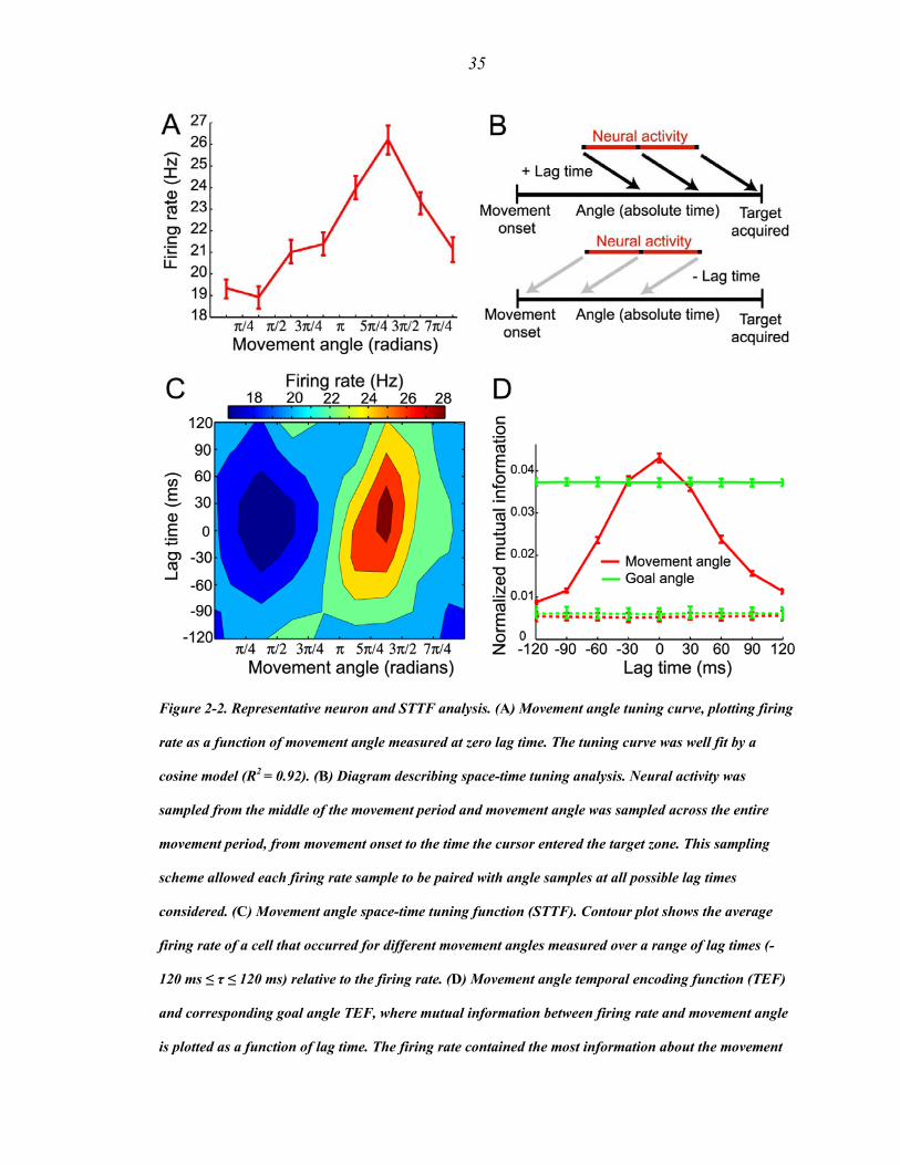
35
Figure 2-2. Representative neuron and STTF analysis. (A) Movement angle tuning curve, plotting firing
rate as a function of movement angle measured at zero lag time. The tuning curve was well fit by a
cosine model (R2 = 0.92). (B) Diagram describing space-time tuning analysis. Neural activity was
sampled from the middle of the movement period and movement angle was sampled across the entire
movement period, from movement onset to the time the cursor entered the target zone. This sampling
scheme allowed each firing rate sample to be paired with angle samples at all possible lag times
considered. (C) Movement angle space-time tuning function (STTF). Contour plot shows the average
firing rate of a cell that occurred for different movement angles measured over a range of lag times (-
120 ms ≤ τ ≤ 120 ms) relative to the firing rate. (D) Movement angle temporal encoding function (TEF)
and corresponding goal angle TEF, where mutual information between firing rate and movement angle
is plotted as a function of lag time. The firing rate contained the most information about the movement

36
angle at an optimal lag time of 0 ms. All error bars denote 95% confidence intervals. Since the target
was stationary during each trial (e.g., goal angle did not change during a trajectory), the goal angle
information was approximately constant across lag time. The dashed lines denote surrogate TEFs, for
both movement (red-dashed) and goal (green-dashed) angles, that were derived from surrogate spike
trains and actual angles. Note that there is no temporal tuning structure in the surrogate movement
angle TEF.
During the center-out task, we recorded from 652 neurons from 2 monkeys. 390 neurons
were significantly tuned for either the movement angle or goal angle, or both. 220/390
(56%) significantly encoded the movement angle and 292/390 (75%) significantly
encoded the goal angle. During the obstacle task, we recorded from 221 neurons from
monkey 1 and 212 of these were significantly tuned for either the movement angle or
goal angle. 168/212 (79%) neurons significantly encoded the movement angle and
197/212 (93%) significantly encoded the goal angle. Since our analysis relies upon the
neural tuning properties being stationary in time, the above population counts do not
include any cells that exhibited non-stationarity (Supporting Information).
Interestingly, we found an anatomical correlate for the representation of goal angle and
movement angle in the medial intraparietal area: the mutual information for goal angle
tended to increase gradually with the depth of the recording electrode, while information
for movement angle (peak information, measured at OLT) decreased with depth. A linear
regression using least squares was performed to quantify a linear relationship between
encoded information and depth, and 100 (1-α) % confidence intervals were obtained for
the slope of the line. The average movement angle information decreased by

37
approximately 30% over a 10 mm span (α = 0.038). The average goal angle information
increased with depth in the sulcus, by about 60%, over 10 mm (α = 0.002). A stronger
encoding of target-related signals deeper in the intraparietal sulcus (IPS) and conversely a
favored representation of arm movement related activity in surface regions of the IPS is
consistent with previous PPC studies of reach planning, in which eye-centered target
signals were commonly found in deeper structures such as PRR, and more hand-related
activity was reported for surface area 5 neurons (C. A. Buneo et al., 2002).
2.3.2 Static encoding of goal angle
Neurons that were significantly tuned for the goal angle persistently encoded information
about the static direction to the target (measured from the starting cursor position, which
is also the fixation point), independent of the changing state of the cursor. These cells
were consistent with previous descriptions of target-sensitive tuning in area 5 (J. Ashe
and A. P. Georgopoulos, 1994). This target representation is most likely not due simply
to a cue response since the neural activity we analyzed typically occurred more than 240
ms after cue onset. Therefore, the intended goal of the trajectory is maintained in the PPC
population during control of the movement. Knowledge of the target direction during the
movement could be used downstream, for example by motor cortices, to adjust upcoming
motor commands to more accurately constrain the trajectory toward the target. Similarly,
a forward model that estimates current and future states of the cursor could also exploit
this online target information to generate more accurate estimates of the state of the
cursor.

38
2.3.3 Temporal encoding of movement angle
PPC neurons tuned for the movement angle encode dynamic information about the
changing state of the cursor. Fig. 2-3A shows TEFs for the entire movement angle
population, normalized on a per cell basis by each cell’s maximal mutual information.
TEFs were typically single-peaked at each cell’s OLT. The histogram in Fig. 2-3B
summarizes the distribution of OLTs for the movement angle population, which was
centered at 0 ± 90 ms and 30 ± 90 ms, for the center-out and obstacle tasks respectively
(median ± interquartile range (IQR)). Both of these plots show that movement angle
neurons contained a temporal distribution of information about the state of the ongoing
movement; some neurons best represented states in the near future (positive-lag time),
some best represented states in the recent past (negative-lag time), and many peaked
around the current state (zero-lag time). Passive sensory feedback would require at least
30-90 ms (proprioceptive-visual) to reach PPC; consistent with some of the negative
OLTs (≤ -30 ms) observed here (M. Flanders and P. J. Cordo, 1989; R. C. Miall et al.,
1993; N. Petersen et al., 1998; S. E. Raiguel et al., 1999). Conversely, if PPC neurons
were encoding an outgoing motor command, subsequent motor processing and execution
of the movement would require at least 90 ms to produce the corresponding cursor
motion, resulting in positive OLTs above 90 ms (R. C. Miall et al., 1993). For instance,
similar analyses for velocity have been performed in the primary motor cortex and report
average OLTs of approximately 90-100 ms (J. Ashe and A. P. Georgopoulos, 1994; L.
Paninski et al., 2004). Therefore, it is unlikely that PPC is driving motor cortex with
feedforward commands since it would be expected that PPC would lead the movement
state by more than motor cortex does, on average (i.e., OLT > 90 ms). Previous studies

39
have reported that velocity information is present in area 5 and suggested that those
neurons best reflect non-causal, sensory information (J. Ashe and A. P. Georgopoulos,
1994; B. B. Averbeck et al., 2005). We performed an additional temporal encoding
analysis for velocity and obtained very similar results to those reported here for
movement angle (Supporting Information). Neither passive sensory feedback nor efferent
motor explanations best account for many of the OLTs observed in our data. In contrast,
the most reasonable description of neurons whose optimal lag times lie between -30 and
90 ms is that they encode a forward estimate, which is used to monitor the current and
upcoming state of the movement angle, prior to the arrival of delayed sensory feedback.
We suggest that these forward state estimates most likely reflect the operation of a
forward model, which relies upon efference copy and a model of the dynamics of the
cursor in order to mimic the causal process that governs how the cursor transitions from
one state to the next.

40

41
Figure 2-3. Population temporal encoding results. (A) Population TEFs plotted for all movement angle
neurons showing cell-normalized mutual information as a function of lag time. TEFs are sorted from
lowest to highest optimal lag time (OLT). The population encoded a distribution of temporal
information, including past, present, and future states of the movement angle. Note that some neurons’
TEFs had more data than others since one monkey made slightly faster movements than the other. (B)
Histogram summarizing the OLTs for movement angle neurons for both center-out and obstacle tasks.
Many of these neurons’ OLTs were consistent with a forward estimate of the state of the movement
angle, which did not directly reflect delayed sensory feedback to PPC, nor were they compatible with
outgoing motor commands from PPC. Color-coded horizontal bars beneath the abscissa denote the
approximate lag time ranges for sensory (blue), forward estimate (black), and motor (red)
representations of the state of the movement angle.
We also observed that the peak information (mutual information at the OLT) encoded by
those neurons that were clearly forward-estimating (0 ≤ OLT ≤ 60 ms) was significantly
larger than the peak information encoded by the remaining population of movement angle
neurons (OLT ≤ -30 ms, or, OLT ≥ 90 ms) (p < 0.001, Wilcoxon rank sum test,
(Supporting Information)). This result shows that, in addition to PPC having a central
tendency to encode the current state of the movement angle, these forward-estimating
neurons will also on average encode more information compared to neurons at other
OLTs, providing further support that the population best represents forward estimates of
the state of the cursor. In addition, we observed that the median OLT for the obstacle task
distribution was significantly larger than the median OLT for the center-out task
distribution, and shifted forward from 0 to 30 ms (p < 1e-4, Wilcoxon rank sum). This
result suggests that during situations in which a more demanding ‘control load’ is placed
on the sensorimotor control system (e.g., the obstacle task), PPC responds by encoding a
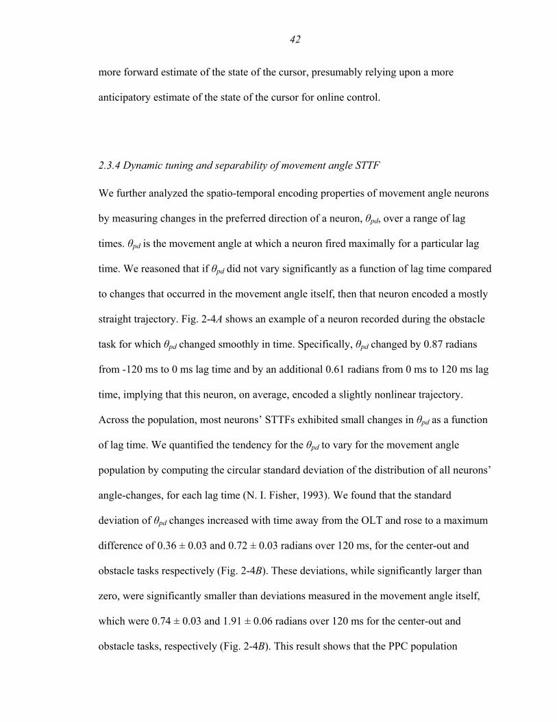
42
more forward estimate of the state of the cursor, presumably relying upon a more
anticipatory estimate of the state of the cursor for online control.
2.3.4 Dynamic tuning and separability of movement angle STTF
We further analyzed the spatio-temporal encoding properties of movement angle neurons
by measuring changes in the preferred direction of a neuron, θpd, over a range of lag
times. θpd is the movement angle at which a neuron fired maximally for a particular lag
time. We reasoned that if θpd did not vary significantly as a function of lag time compared
to changes that occurred in the movement angle itself, then that neuron encoded a mostly
straight trajectory. Fig. 2-4A shows an example of a neuron recorded during the obstacle
task for which θpd changed smoothly in time. Specifically, θpd changed by 0.87 radians
from -120 ms to 0 ms lag time and by an additional 0.61 radians from 0 ms to 120 ms lag
time, implying that this neuron, on average, encoded a slightly nonlinear trajectory.
Across the population, most neurons’ STTFs exhibited small changes in θpd as a function
of lag time. We quantified the tendency for the θpd to vary for the movement angle
population by computing the circular standard deviation of the distribution of all neurons’
angle-changes, for each lag time (N. I. Fisher, 1993). We found that the standard
deviation of θpd changes increased with time away from the OLT and rose to a maximum
difference of 0.36 ± 0.03 and 0.72 ± 0.03 radians over 120 ms, for the center-out and
obstacle tasks respectively (Fig. 2-4B). These deviations, while significantly larger than
zero, were significantly smaller than deviations measured in the movement angle itself,
which were 0.74 ± 0.03 and 1.91 ± 0.06 radians over 120 ms for the center-out and
obstacle tasks, respectively (Fig. 2-4B). This result shows that the PPC population

43
encoded significantly less change in movement direction than was observed in the actual
trajectories themselves (< 50%). We also calculated the average curvature of the
monkeys’ trajectories and the curvature of simulated trajectories derived from a neuron’s
STTF, which were considered to be the ‘preferred trajectory’ of a neuron. Consistent with
the preferred direction results, the average curvature of preferred trajectories (0.06 ± 0.01
and 0.15 ± 0.04, for center-out and obstacle tasks, respectively) was significantly less
than the average curvature of the actual trajectories (0.15 ± 0.04 and 0.26 ± 0.02, for
center-out and obstacle tasks respectively). This result further substantiates the claim that
movement-related neurons encoded mostly instantaneous straight-line trajectories, which
contained less curvature than was present in the actual executed movements.
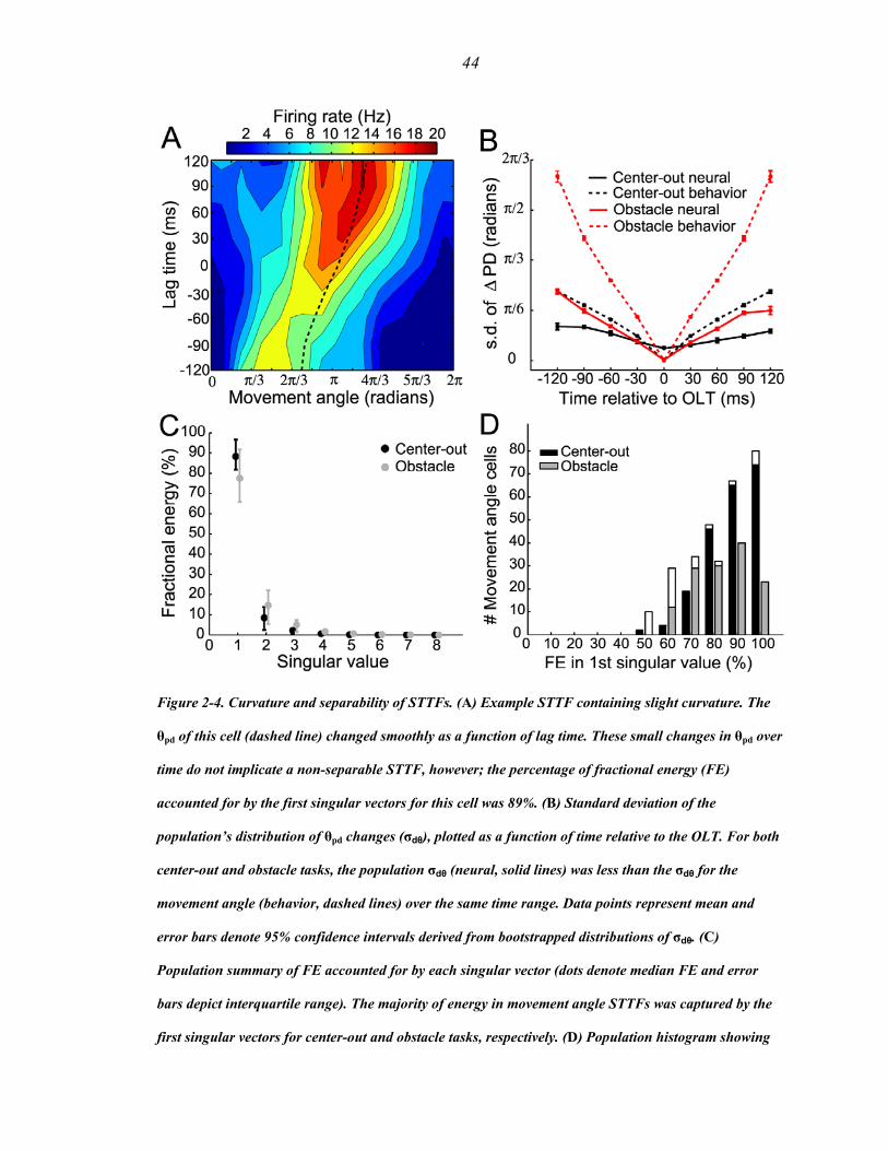
44
Figure 2-4. Curvature and separability of STTFs. (A) Example STTF containing slight curvature. The
θpd of this cell (dashed line) changed smoothly as a function of lag time. These small changes in θpd over
time do not implicate a non-separable STTF, however; the percentage of fractional energy (FE)
accounted for by the first singular vectors for this cell was 89%. (B) Standard deviation of the
population’s distribution of θpd changes (σdθ), plotted as a function of time relative to the OLT. For both
center-out and obstacle tasks, the population σdθ (neural, solid lines) was less than the σdθ for the
movement angle (behavior, dashed lines) over the same time range. Data points represent mean and
error bars denote 95% confidence intervals derived from bootstrapped distributions of σdθ. (C)
Population summary of FE accounted for by each singular vector (dots denote median FE and error
bars depict interquartile range). The majority of energy in movement angle STTFs was captured by the
first singular vectors for center-out and obstacle tasks, respectively. (D) Population histogram showing

45
distribution of FE of first singular value for all movement angle cells. Unfilled (white) regions of bars
denote fraction of cells that were not significantly separable. Overall, the distributions for the two tasks
were largely separable.
We performed an additional separability analysis to further characterize the relationship
between angle and lag time encoded by a neuron’s STTF. A perfectly separable STTF
indicated that lag time and angle were encoded independently of one another. We
determined that the population of movement angle neurons was largely separable in the
angle-time plane by using singular value decomposition (SVD) (J. L. Pena and M.
Konishi, 2001; J. A. Mazer et al., 2002). We calculated the fractional energy contained in
the singular values for each cell’s movement angle STTF. 92.0 ± 14.7% and 78.9 ±
25.8% of energy (median + IQR) was contained in the first singular value, for the center-
out and obstacle tasks, respectively (Fig. 2-4C). 209/220 (95%) and 130/168 (77%) of
movement angle STTFs were significantly separable when compared to their
corresponding surrogate STTFs, for center-out and obstacle tasks. Fig. 2-4D shows the
distribution of fractional energies of the first singular value for both tasks. These SVD
results show that movement angle and time were primarily encoded independently by the
PPC population and suggest that they could be combined in a multiplicative fashion to
create the observed STTFs.
Together, the above analyses suggest that dynamic sensorimotor control mechanisms in
PPC encode mostly straight trajectories, with a less substantial component of neurons’
firing rates arising due to nonlinear encoding mechanisms that may reflect the slight
curvature we observed in the STTFs. This interpretation is consistent with PPC neurons

46
encoding a state estimate of the movement angle, such that the majority of information is
encoded at a cell’s OLT, with decreasing information encoded away from the OLT.
2.4 Discussion
Our data suggest that neurons in PPC are not only involved in forming plans for
movement (L. H. Snyder et al., 1997; R. A. Andersen and C. A. Buneo, 2002b), but also
in monitoring the goal and the dynamic state of the trajectory during movement
execution. This monitoring is likely important for, among other purposes, continuous
control and error correction. Rapid online control of movement cannot rely completely
upon slow sensory feedback but instead must make continuous adjustments to motor
commands based upon a best estimate of the current and future states of the effector (R.
C. Miall and D. M. Wolpert, 1996; M. Desmurget and S. Grafton, 2000). The temporal
encoding properties of many movement angle neurons suggest that PPC computes an
estimate of the state of the cursor forward in time, consistent with the operation of a
theoretical forward model. Furthermore, the distribution of OLTs we report in PPC spans
a continuum of dynamic state estimates, bridging purely sensory with purely motor
representations of the state of a continuous movement, while having a central tendency to
encode a forward estimate of the current state of the cursor. We suggest that PPC
movement angle neurons may provide a sensorimotor linkage necessary for translating
desired goals and anticipated errors measured in the sensory domain into appropriate
motor commands necessary for accurate and rapid control of the limb (M. I. Jordan and
D. E. Rumelhart, 1992; R. C. Miall and D. M. Wolpert, 1996). It should be noted that the
forward estimate measured using our analysis corresponds to the expected movement
47
state of an external object (i.e., the sensory outcome of the cursor motion on the computer
screen). However, for our joystick task, the movement of the cursor is strongly correlated
with the movement of the hand, and therefore it is also possible that these state estimates
might reflect an intrinsic representation of the hand itself. Further experiments should be
carried out to determine to what extent the forward model in PPC encodes a motor,
sensory (visual and/or proprioceptive) or intermediate representation of the expected state
of a movement.
A forward model must rely both upon efference copy and a model of the dynamics of the
cursor/hand to estimate the next state of a movement from the previous state. Efference
copy signals could be central in origin (fed back from motor and premotor cortices) or
may be signals of non-cortical origin that lead the current state of the movement.
Previous psychophysical, clinical and theoretical studies have pointed to both the parietal
lobe and the cerebellum as candidate neural substrates for a forward model (D. M.
Wolpert et al., 1998a; D. M. Wolpert et al., 1998b; S. J. Blakemore and A. Sirigu, 2003;
A. J. Bastian, 2006). Since both areas are reciprocally connected (cerebellum projects to
parietal cortex via the thalamus (D. M. Clower et al., 2001); parietal cortex projects to
cerebellum via the pons (M. Glickstein, 2000)), it is quite possible that the two areas
might comprise a ‘functional loop’ responsible for monitoring and updating the internal
state of the limb for online control (S. J. Blakemore and A. Sirigu, 2003). The extent to
which forward model control is distributed across multiple brain areas and the
distinguishing functional roles of these areas is an important direction for further
investigation.

48
The finding that movement angle neurons are largely separable in the angle-time plane
implies that online directional tuning is mostly stable over time during the movement.
While PPC neurons do encode some curvature during our tasks, both the average change
in θpd (approximately π/6 radians in 120 ms) and the amount of curvature encoded by
PPC neurons were not large and moreover were both significantly smaller than their
corresponding values measured for the movement itself over the same time range.
Therefore, these ‘preferred trajectories’ are not complex functions of time but for the
most part provide a simple dynamic encoding scheme: state estimation of movement
direction at a particular OLT. This explanation is conceptually similar to the claim that
M1 neurons encode an instantaneous estimate of movement direction (or velocity) at a
particular lag time (A. B. Schwartz et al., 1988; D. W. Moran and A. B. Schwartz, 1999).
Alternatively, Hatsopoulos and colleagues have recently suggested that neurons in M1
encode more complex ‘pathlets’, which are comprised of a broad range of temporally
extensive trajectory shapes (N. G. Hatsopoulos et al., 2007). This complex spatio-
temporal encoding scheme may in part reflect M1’s involvement in the execution of
actions in coordinate frames appropriate for musculoskeletal control, although a single
coordinate frame for M1 has not been identified (W. Wu and N. Hatsopoulos, 2006). In
contrast, we suggest that the encoding of space and time that we observe in PPC may best
reflect a visuomotor representation of the trajectory, which seems reasonable given the
strong sensory input to PPC as well as its substantial reciprocal connections with
downstream motor areas (E. G. Jones and T. P. Powell, 1970; P. B. Johnson et al., 1996).

49
A representation of the expected state of the cursor may also be useful for reconciling
whether the outcome of a movement in space is caused by self-induced or external
sensory motion. PPC would be a reasonable brain area to perform such a reafference-
cancelling computation during continuous sensorimotor control given both the presence
of a forward model estimate of the sensory consequences of movement and the
convergence of substantial sensory inputs. Unfortunately, since the desired sensory
outcome and the actual sensory outcome of the movement coincide closely in our task,
we cannot determine from our data whether a comparison between these two signals is
encoded in PPC or not. A future experiment that perturbs the cursor visual feedback so
that it is incongruent with the movement of the joystick, dissociating the intended
movement state and the actual visual state, might modulate the activity of cells that did
not respond during our task, which would normally encode such a comparison.
Eye-behavior-related signals have also been described previously in PPC (V. B.
Mountcastle et al., 1975). For instance, some smooth pursuit sensitive cells in area MST
appear to reflect the integration of an extraretinal signal related to the continuous
movement of the eye, and continue to respond during periods of the pursuit when the
stimulus is blinked off (W. T. Newsome et al., 1988). One use of this signal may be for
perceptual stability during pursuit eye movements (D. C. Bradley et al., 1996; T.
Haarmeier et al., 2001). It would be interesting to determine whether MST cells estimate
the current direction of eye movements during pursuit, similar to the forward estimation
of movement angle we observe for arm movements. Discrete eye behavior related
signals, such as saccade and fixation responses have also been described in PPC.

50
Whereas area 7a saccade responses begin largely after the saccade, area LIP saccade
responses tend to occur before, during or after saccades (R. A. Andersen et al., 1987).
These dynamics have led to the suggestion that this saccade activity is important for
perceptual stability and coordinate transformations, but not for the execution of eye
movements (R. A. Andersen et al., 1987). (Note that although LIP does not appear to
generate the execution signal for saccades, it does appear to be involved in the
formulation of the plan or intent to saccade (R. A. Andersen and C. A. Buneo, 2002a)).
The saccade response dynamics in LIP appear to estimate when a saccade is occurring.
Fixation-related activity commonly found in PPC is sensitive for eye position, and this
response characteristic is often multiplicatively combined with the sensory and saccade-
related activity of single neurons (R. A. Andersen et al., 1987). The eye position signal in
the posterior parietal cortex could be derived from proprioceptive inputs from the eye
muscles (X. L. Wang et al., 2007) and/or the integration of saccade command signals. It
would be interesting to see if a component of the eye position signal might also provide
anticipatory information (ahead of passive sensory feedback) about the current state of
the eye position during fixations between saccades.
Finally, the availability of both goal and dynamic arm movement information in PPC
make this brain area an attractive target for a neural prosthesis. For example, a continuous
decoder estimating the dynamic state of the cursor could be improved by incorporating
target information to constrain the decoded cursor trajectory toward the goal (L.
Srinivasan and E. N. Brown, 2007). Moreover, at any instant during the movement, the
trajectory decoder could be switched to a target decoder when sufficient information
51
becomes available about the target, rapidly jumping the cursor to the correct endpoint.
Lastly, the observation that these neurons appear to encode mostly straight lines in visual
space may prove to be more straightforward to decode for controlling a variety of end
effectors.
2.5 Methods
In our experiment, 2 monkeys were trained to perform a 2D center-out joystick (ETI
Systems) reaction task. Both monkeys performed a center-out task and the first monkey
was also trained to perform an obstacle avoidance task to enforce more curvature in the
trajectories and to further de-correlate goal angle and movement angle (center-out task
correlation coefficient: ρT = 0.70 ± 0.06., ρT = 0.57 ± 0.12 for monkeys 1 and 2,
respectively, obstacle task: ρT = 0.16 ± 0.11, (mean ± standard deviation (s.d.)), T-linear
association test (N. I. Fisher, 1993)). Example trajectories are shown for both tasks in
Fig. 2-1 C and D. During joystick trials, we recorded simultaneous single-unit activity
from multiple neurons (up to 4-channels) in the medial bank of the intraparietal sulcus of
the posterior parietal cortex (PPC), with chamber coordinates centered at 5 mm posterior
and 6 mm lateral.
2.5.1 Behavioral task
The monkeys sat 45 cm in front of an LCD monitor. Eye position was monitored with an
infrared oculometer (ISCAN Inc.). The monkeys initiated a trial by moving a white
cursor (0.9 degrees (deg)) into a central green target circle (4.4 deg) and then fixated a
red concentric circle (1.6 deg). After 350 ms, the target was jumped to 1 of 8 (or 12)

52
random peripheral locations (14.7 deg). The monkeys then guided the cursor smoothly
into the peripheral target while maintaining central fixation. Once the cursor was held
within 2.2 deg of the target center for 350 ms, the monkeys were rewarded with a drop of
juice. In the obstacle task, the monkey initiated the trial as before. After 350 ms, a blue
obstacle circle (10.0 deg) appeared and the target was jumped simultaneously to 1 of 8
(or 12) target locations. The obstacle was aligned and equidistant between initial and final
target positions. During movement, the monkey maintained central fixation and guided
the cursor around the obstacle and into the peripheral target. If the cursor intersected the
obstacle or fixation was broken, the trial was aborted. The duration from movement onset
to the time the cursor entered the target was for the center-out task: 259 ± 80 ms and 392
± 173 ms for monkeys 1 and 2 respectively, and for monkey 1 for the obstacle task: 360 ±
99 ms (mean ± s.d.)).
2.5.2 Space-time tuning analysis
Spike trains and raw joystick positional data were smoothed with a Gaussian kernel (s.d.
= 20 ms). The standard deviation of the smoothing Gaussian was derived from the
standard deviation of the inter-spike interval (ISI) distribution of a typical neuron.
Specifically, a Gaussian curve was fit to every tuned neuron’s ISI distribution. The
median ISI standard deviation for all neurons was 23 ms, which we then approximated to
20 ms.
We evaluated the dynamic tuning properties of PPC neurons by constructing a space-time
tuning function (STTF) for each neuron, described by the bivariate function N(θ,τ) (L.

53
Paninski et al., 2004). Each value in the STTF represented the expected value of the
firing rate, R, measured at some time during the movement, t, given that a particular
behavioral angle, θ, occurred at time t + τ. The STTF is then expressed as the conditional
expectation
[ ])(|),( τθτθ REN = [1]
where τ is the lag time, which was sampled in 30 ms increments, and E is the expected
value operator. To compute the average firing rate for a particular STTF bin, N(θbin,τbin),
firing rate samples were accumulated at all times{ti} for which θ = θbin at times {ti+ τ },
and across all trials in a session. This sum was then divided by the total number of firing
rate samples that occurred for that θbin-τbin bin, to give an average firing rate. Both goal
and movement angle bins were discretized into π/4 radians increments (π/6 radians, for
12-target experiments), while firing rates were binned into 1 Hz increments. We tried a
variety of bin-size resolutions for both parameters, none of which had any qualitative
effect on the results reported in this study. On average, more than 70,000 firing rate
samples were used per session, which were compiled over 489 ± 300 and 498 ± 233 trials
(mean ± s.d.), for the center-out and obstacle tasks respectively (typically resulting in >
500 samples per θ-τ bin and > 40 trials per target).
The movement angle and goal angle were sampled every millisecond over the entire
trajectory, from movement onset to the instant the cursor entered the target circle.
Importantly however, firing rates were sampled from the middle segment of a trial so that
each firing rate sample could be paired with angles sampled uniformly over the entire
range of lag times we considered (Fig. 2-2B). This eliminated unwanted edge effects for

54
large-magnitude values of lag time (e.g., a sampling bias would otherwise exist for say τ
= -120 ms; firing rates would be more likely to be sampled from later times in the
trajectory and these samples would be less likely to have corresponding angle pairs for τ
> 0). This segment of neural activity varied in size depending upon the trial length, and
on average was 145 ± 22 ms and 147 ± 18 ms (mean ± s.d), for the center-out and
obstacle tasks, respectively. In addition, we only considered firing rates beginning from
90 ms after movement onset to allow sufficient time for sensory feedback about the state
of the movement to arrive into PPC. This was important to ensure that none of the PPC
neural activity we reported reflected encoding schemes that operated without access to
visual or proprioceptive feedback during online control of the cursor. Finally, it is
unlikely that this neural activity period reflected stimulus onset or reward since it began
more than 220 ms (reaction time + at least 90 ms) after cue onset and terminated more
than 440 ms (350 ms hold + at least 90 ms) before reward delivery. The reaction time to
initiate movement was 138 ± 51 ms and 159 ± 19 ms (mean ± s.d.), for the center-out and
obstacle tasks, respectively.
A bootstrap Monte Carlo re-sampling method (> 100 iterations) was used to generate a
distribution of STTFs, which were averaged to yield the reported STTF, and from which
we derived 95% confidence intervals. To create a null hypothesis for significance testing,
we constructed surrogate STTFs by using actual trajectory data (to preserve kinematics)
but by substituting neural activity with surrogate spike trains. Surrogate spike trains were
generated by sampling uniformly from a neuron’s actual inter-spike interval distribution
(i.e., surrogate neurons contained the same ISI spiking statistics and mean firing rate as

55
the actual neurons), and then subsequently smoothing the surrogate spike train as before.
Using this surrogate neural activity and the actual behavior (movement or goal angles),
bootstrap Monte Carlo re-sampling was performed again to create a distribution of
surrogate STTFs.
Cosine goodness-of-fit was also assessed for all lag times in a neuron’s STTF (i.e., an
angular tuning curve for each lag time) according to the following model
[2] )cos(*)( pdτ acN θθθ −+=
where c is the baseline firing rate, a is the gain, θpd is the preferred direction of the
neuron, and Nτ denotes the angular tuning function for a particular lag time. This model
typically provided a good fit for the population of movement angle neurons. The
coefficient of determination, R2, for the model fit was 0.70 ± 0.43 and 0.83 ± 0.19 (mean
± s.d.), for the center-out and obstacle tasks, respectively. θpd was computed using the
mean direction method (N. I. Fisher, 1993). Specifically, vector addition was used to
determine the resultant vector, B, at which a cell fired maximally for a given lag time as
follows
BSBC
BSCBNSNC
pdpd
M
i
M
iiiii
==
≥+=== ∑ ∑= =
θθ
θθ
sin , cos
0 ,sin ,cos1 1
222
[3]
where M is the number of angle bins (8 or 12) and Ni is a neuron’s average firing rate for
a particular bin angle, θi.

56
Note that the STTFs we report here differ somewhat from the spatio-temporal receptive
fields used in sensory cortices, which generally use white noise stimuli to probe a rich set
of space-time representations (N. Kowalski et al., 1996; G. C. DeAngelis et al., 1999).
Due to autocorrelation present in natural goal-directed arm movements, we do not
interpret the structure of STTFs to represent what is directly encoded by PPC neurons for
all possible stimuli, but instead to reflect the movement angle dynamics that can be
inferred from the firing rate for our particular task.
2.5.3 Information theoretic analysis
Because tuning depth and linear correlation metrics such as Pearson’s linear correlation
coefficient are not a robust measure of all types of statistical dependency, we calculated
the Shannon mutual information between firing rate and angle for each lag time of the
STTF to construct a temporal encoding function (TEF) (T. M. Cover and J. A. Thomas,
1991; L. Paninski et al., 2004). This method allowed us to rigorously quantify the
dependency of the firing rate on the movement or goal angle at different lag times.
Mutual information is an entropy-based measure that quantifies how much the variability
of a particular parameter (i.e., neural firing rate, N) is dependent upon the variability of
another (i.e., goal or movement angle, θ), and is defined as
⎟⎟⎠
⎞⎜⎜⎝
⎛= ∫ ∫ )(
)|(log)|()();(θ
θθθθ p
NpNpNpNIN
. [4]
p(N) is the prior probability distribution for firing rates. p(θ|N) is the conditional
probability distribution for angle given that a particular firing rate was observed. p(θ) is
the prior probability distribution for angle. We computed the above integral using a non-
57
parametric binning approach. Specifically, we did not approximate these distributions
using a model fit but instead computed them exactly by evaluating the integral in Eq. 4 as
a finite sum according to
( ) ( )( )∑ ∑ ⎟⎟
⎠
⎞⎜⎜⎝
⎛=
N pNpNpNpNI
θ θθθθ |log|)();( . [5]
To ensure that mutual information values for goal and movement angle were comparable
(e.g., to avoid any bias due to possible differences in the individual goal angle or
movement angle entropies), we normalized mutual information using the symmetric
uncertainty measure introduced by Särndal (C. E. Sarndal, 1974)
( ) ( )( ) ( )θ
θθHNH
NINNI+
⋅=
;2; . [6]
The normalized information, NI, effectively varied between 0 and 1, with NI = 1
denoting perfect correlation. H(θ) and H(N) are the entropy of the angle (goal or
movement) and the firing rate, respectively, and were computed in a similar manner - for
example:
( ) ( ) ( )∑−=θ
θθθ ppH log . [7]
Therefore, the NI scalar quantity was not reported in bits, but should instead be
interpreted simply as a non-parametric measure of dependency of the firing rate on the
angle.
Note that goal angle TEFs were mostly flat and did not contain temporal encoding
structure (e.g., Fig 2-1D). This is because for any given trial, all firing rate samples in the
neural activity period were paired with the same goal angle (i.e., a single target) at all
possible lag times. Therefore, each trial contributed only a mean rate for one particular

58
goal angle, with no temporal information. When repeated across all trials, the resultant
goal angle STTF contained angular tuning but no temporal tuning, resulting in a flat TEF.
Importantly, a flat TEF does not imply that goal angle information was fixed in absolute
trial time, but instead represents the average tuning strength for target direction during the
neural activity period that we sampled.
2.5.4 Temporal dynamics and curvature of movement angle STTF
To assess how the encoded movement angle varied as a function of lag time, the
difference between θpd at a cell’s OLT and θpd at all other significantly tuned lag times
was calculated for a neuron’s STTF. This calculation was carried out for all cells that had
significantly tuned lag times in the range of -120 to 120 ms. So that we could compare
these changes in θpd with changes that occurred in the movement angle itself, we also
calculated the difference between the movement angle for all times {ti} and the
movement angle at all times {ti+ τ}, for a range of different lag times (-120 ≤ τ ≤ 120
ms). This process was then repeated for all trials in a session and for all sessions in which
movement angle neurons were reported. These procedures resulted in a distribution of
angle-differences associated with each lag time, both for the neural activity (i.e., changes
in θpd) and the behavior (i.e., changes in movement angle) (Fig 2-4B). We then computed
the circular standard deviation, σdθ, for each lag time’s distribution of angle-differences
(N. I. Fisher, 1993) to summarize the average tendency of the angle to deviate over lag
time. A bootstrap Monte Carlo re-sampling procedure was used to generate multiple
distributions of angle-differences, from which the mean and 95% CIs for σdθ were
derived (Fig. 2-4B).

59
In addition to the preferred direction analysis, we calculated the curvature of both the
actual trajectories themselves and a neuron’s preferred trajectory, which we simulated
from a neuron’s STTF. First, to derive the curvature of an actual trajectory, a circle was
fit to a series of points sampled every 30 ms along a 240 ms trajectory segment using a
non-linear least squares estimation approach presented by Gander and colleagues in (W.
Gander et al., 1994) and implemented in the Matlab program, ‘fitcircle’, by R. Brown
(University of Canterbury). The curvature was then calculated simply as the inverse of
the radius of the circle. This calculation was repeated for a series of subsequent 240-ms
trajectory segments within each trial, each beginning 30 ms apart (i.e., 0-240 ms, then 30-
270 ms …), and then repeated for all trials in a session. Second, to construct the
‘preferred trajectory’ encoded by a neuron’s STTF, we combined unit vectors, which
were derived from each lag time’s θpd, in a tip-to-tail fashion from -120 ms to +120 ms.
The curvature of the resultant trajectory was then computed as described above and then
this procedure was repeated for each neuron in the population.
2.5.5 Separability of movement angle STTF
To assess the separability of an STTF, using SVD we modeled the movement angle
STTF matrix N as a function of an offset term plus a multiplicative component
[8] TUSVN +=α
where U and V are orthogonal matrices containing the singular vectors and S is a diagonal
matrix containing the nonzero singular values of N. If an STTF was completely

60
separable, then it could be factored using only the first singular vectors and first singular
value
[9] TvsuN 111+=α
with s1=1 denoting that all energy could be captured in the space spanned by the first
singular vectors. Varying α from the minimum to the maximum firing rate of a neuron (in
increments of 1 Hz), we iteratively fit the separable model of Eq. 9 to reconstruct the
matrix N. This optimization process allowed us to determine the optimal offset, αopt,
which minimized the mean squared error for reconstructing N, similar to the approach of
Pena and colleagues (J. L. Pena and M. Konishi, 2001). Typically, we found that αopt was
strongly correlated with the mean value of the N matrix (correlation coefficient, ρcc = 0.97
and ρcc = 0.90, for center-out and obstacle tasks). Using αopt, the full SVD decomposition
was then performed once more according to Eq. 8 and the fractional energy (FE)
contained in each set of singular vectors was calculated as
∑⋅=
ii
ii s
sFE 2
2
%100 . [10]
To determine whether or not the FE contained in the first singular value was significantly
separable, we also performed SVD decomposition on surrogate STTFs, (which were
derived from the same behavior but using surrogate spike trains) for comparison with the
actual STTFs’ separability. If the first singular value computed from the actual STTF was
larger than 95% of the surrogate STTF’s first singular values, then the SVD
decomposition was considered to be significantly separable.

61
Acknowledgements
We thank R. Bhattacharyya, E. Hwang, I. Kagan and Z. Nadasdy for comments on the
manuscript, K. Pejsa and N. Sammons for animal care, and V. Shcherbatyuk and T. Yao
for technical and administrative assistance. This work was supported by the National Eye
Institute, the James G. Boswell Foundation, the Defense Advanced Research Projects
Agency (DARPA), and an NIH training grant fellowship to G.H.M.
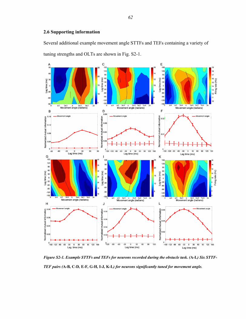
62
2.6 Supporting information
Several additional example movement angle STTFs and TEFs containing a variety of
tuning strengths and OLTs are shown in Fig. S2-1.
Figure S2-1. Example STTFs and TEFs for neurons recorded during the obstacle task. (A-L) Six STTF-
TEF pairs (A-B, C-D, E-F, G-H, I-J, K-L) for neurons significantly tuned for movement angle.
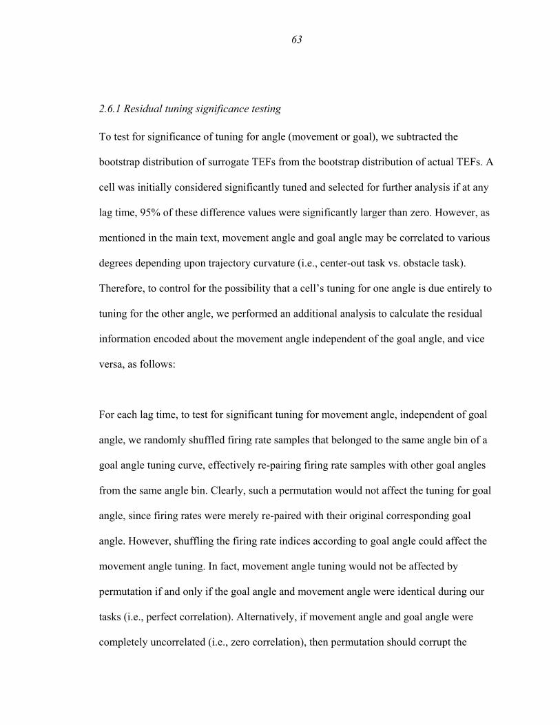
63
2.6.1 Residual tuning significance testing
To test for significance of tuning for angle (movement or goal), we subtracted the
bootstrap distribution of surrogate TEFs from the bootstrap distribution of actual TEFs. A
cell was initially considered significantly tuned and selected for further analysis if at any
lag time, 95% of these difference values were significantly larger than zero. However, as
mentioned in the main text, movement angle and goal angle may be correlated to various
degrees depending upon trajectory curvature (i.e., center-out task vs. obstacle task).
Therefore, to control for the possibility that a cell’s tuning for one angle is due entirely to
tuning for the other angle, we performed an additional analysis to calculate the residual
information encoded about the movement angle independent of the goal angle, and vice
versa, as follows:
For each lag time, to test for significant tuning for movement angle, independent of goal
angle, we randomly shuffled firing rate samples that belonged to the same angle bin of a
goal angle tuning curve, effectively re-pairing firing rate samples with other goal angles
from the same angle bin. Clearly, such a permutation would not affect the tuning for goal
angle, since firing rates were merely re-paired with their original corresponding goal
angle. However, shuffling the firing rate indices according to goal angle could affect the
movement angle tuning. In fact, movement angle tuning would not be affected by
permutation if and only if the goal angle and movement angle were identical during our
tasks (i.e., perfect correlation). Alternatively, if movement angle and goal angle were
completely uncorrelated (i.e., zero correlation), then permutation should corrupt the

64
tuning for movement angle entirely. However, since goal and movement angles were
partially correlated in our tasks, we observed instead that tuning strength for movement
angle decreased after permutation of the firing rate samples. Therefore, any decrease in
the movement angle mutual information that resulted from shuffling represented
information that the cell encoded about movement angle, and not the goal angle. If this
difference, which we refer to as the residual movement angle information, was
significantly larger than its null hypothesis (generated in an analogous manner, but using
surrogate spike trains) for any lag time, then the cell was considered to significantly
encode movement angle, independent of its tuning for goal angle. If not, then it was
unclear if the cell encoded movement angle and it was excluded from the movement
angle population. Fig. S2-2 shows two different examples of cells’ residual TEFs, one
which was significantly larger than its residual null hypothesis (Fig. S2-2, A) and another
which was not (Fig. S2-2, B). An analogous procedure was used to assess residual tuning
for goal angle. Note, we computed the residual TEF only to ensure that movement angle
tuning could not be trivially explained by its correlation with goal angle. Importantly
however, for OLT analysis we did not use the residual TEF, but instead used the full TEF
described initially, since it is possible that movement angle tuning could be a function of
an interaction between movement angle and goal angle, which the residual tuning
measure does not reflect.
65
Figure S2-2. Example residual movement angle TEF plots. (A) The residual information is lower than
the full movement angle information, but is still significantly above its residual noise level. Therefore,
this cell significantly encoded the movement angle, independent of the goal angle. (I) A second example
showing a cell that was no longer significantly tuned for movement angle after calculating the residual
information.
2.6.2 Peak mutual information as a function of optimal lag time
Fig. S2-3, A and B, plots the peak mutual information that each cell encoded for
movement angle at its OLT, for both the center-out and obstacle tasks. First, notice that
the center-of-mass values, -6 ms and 15 ms, for the center-out and obstacle distributions,
respectively, were consistent with the median OLTs reported in Fig. 2-3B. This was of
course due largely to the higher proportion of cells’ having OLTs near 0 ms, as illustrated
in Fig. 2-3B, but also to the larger amount of information encoded by neurons with OLTs
close to zero lag, as mentioned in the main text. Specifically, during the center-out task,
clearly forward-estimating neurons’ (0 ms ≤ OLT ≤ 60 ms) mutual information was 0.043
± 0.04, compared to 0.036 ± 0.03 for movement angle neurons with other OLTs (OLT ≤ -
30 ms, or, OLT ≥ 90 ms). Similarly, for the obstacle task, the average peak information

66
of clearly forward-estimating neurons was 0.043 ± 0.03, while it was 0.034 ± 0.03 for
movement angle neurons with other OLTs.
Figure S2-3. (A-B) Population summary of peak mutual information encoded at a neuron’s OLT for the
movement angle population during center-out (A) and obstacle tasks (B). Error bars represent standard
deviation of points at each OLT.
2.6.3 Neural stationarity
It is important to show that the neural activity we measured was stationary over the time
period for which we calculated mutual information. Therefore, we evaluated the
stationarity of a neuron’s firing rate during a trial and over an experimental session,
similar to the approach taken by Paninski and colleagues (L. Paninski et al., 2004).
First, we analyzed trends in the firing rate over the course of a session. The average firing
rate was computed for each trial in a session, and the resulting trend in firing rate over the
course of that session was fit by a line. The slope of the line and the percentage change in
the firing rate across the session (from beginning to end) were derived from this fit. For
67
consistency with the literature, we used the criteria of Paninski and colleagues to
determine neural stationarity: if a cell’s firing rate changed by less than 20% during the
session or if the slope of the line fit was not significantly different from zero, the cell was
deemed stationary. If both criteria failed to be met, an additional tuning analysis was
performed to determine whether the actual STTF of the neuron changed significantly
over the course of the session. To do this, we divided the experiment into two parts, and
constructed the STTFs and pseudo-STTFs for both the first (A) and second (B) halves of
the session. Bootstrap Monte Carlo re-sampling methods were used to generate a
distribution of STTFs in the same manner as before. To quantify a change in tuning, we
calculated the sum of squared differences between the bin values in STTFB and STTFA
matrices as well as for the surrogate matrices, S_STTFB and S_STTFA. If the sum of
squared difference between the actual STTFs was larger than 95% of the surrogate sum
of squared differences, the cell was considered non-stationary and was excluded from the
population. Using the above criteria, we found that the population was largely stationary;
220/221 and 168/170 movement angle cells had stationary firing properties over the
course of a session.
To analyze the intra-trial stationarity of the firing rate, we aligned each trial to the
reaction time and then computed the trial-averaged firing rate as a function of elapsed
time. A line was fit to this trend and the slope of the line and the percentage change in the
firing rate were computed. To assess statistical significance of the mean trial slope, 100
bootstrap reshufflings were performed in which the firing rate time series was randomly
shuffled, corrupting any trend in the firing rate over time but preserving its mean value. If
68
the absolute value of the slope of the firing rate trend was larger than 95% of the
bootstrap absolute-value slopes, and the percentage change in the firing rate trend
changed by more than 20%, the cell could be considered non-stationary. We found that
104/220 (47%) and 73/168 (44%) movement angle neurons, in the center-out and
obstacle tasks, respectively, could be considered non-stationary based on this criteria.
However, it is unlikely that these intra-trial firing rate trends reflected any change that
was related to the kinematics of the movement. First, any non-stationarity observed in the
firing rate was not due to non-stationarity in the movement angle itself since the
movement angle was almost always stationary over the course of the trial. Specifically,
for 216/220 and 167/168 of the recorded sessions, the movement angle was determined to
be stationary over the course of the trial based on the same criteria used above to assess
intra-trial neural stationarity. Moreover, we consistently observed cells that exhibited
firing rate trends that increased for some trials and decreased for other trials under
identical target conditions. Furthermore, simultaneously recorded cells frequently had
opposite slopes for the same trial, also suggesting that any non-stationarity in the
movement kinematics was not the cause of these trends in firing rate. While it is possible
that some of the cells we report on may also encode variables that we are not measuring
or that are unrelated to the kinematics in our task, this does not limit the conclusions
being drawn about correlations between neural activity and the movement angle.
2.6.4 Optimal lag time statistical analysis
We performed an additional analysis to determine whether the mutual information
encoded for movement angle at a cell’s OLT was significantly larger than at all other lag
69
times. Our null hypothesis was that the difference between the mutual information at the
OLT and the mutual information at other lag times was not significantly different from
zero. Bootstrapped values of mutual information at each lag time were subtracted from
the mutual information at a cells’ OLT. For each lag time comparison, if 95% of these
differences were larger than zero, then the null hypothesis was rejected and the mutual
information at the OLT was concluded to be significantly larger than the mutual
information encoded at the compared lag time. The outcome of all of these comparisons
is summarized graphically in the 95% confidence OLT plots of Fig. S2-4, where
horizontal error bars delineate the lag time range (30, 60, 90 … ms) within which the
OLT could be claimed to reside with at least 95 % confidence. 160/220 (73%) and
154/168 (92 %) of movement angle neurons, for the center-out and obstacle tasks,
respectively, have OLT confidence intervals less than 90 ms wide, suggesting that most
neurons typically encode a strong dynamic estimate of the state of the movement angle.
Note that we would not expect the temporal resolution of state-estimating neurons to
consistently approach very small values due to implicit autocorrelation in the movement
angle itself (movement angle time constant <140 ms). Importantly however, over a
variety of confidence interval sizes (i.e., temporal resolutions), these plots show that the
central tendency of the population was to consistently encode the recent, current or
upcoming state of the movement angle.

70
Figure S2-4. 95% Confidence intervals for OLT distribution. (A-C) Center-out OLT 95% confidence
intervals are shown for cells for which the OLT is defined with 30 ms (A), 60 ms (B) and 90 ms (C)
temporal precision. Extent of horizontal lines denotes the 95% confidence interval of the OLT. Filled
dots represent the mean OLT for a given confidence interval. Text in upper-right hand corner notes the
median ± interquartile range OLT for each temporal precision plot. (D-F) Obstacle OLT confidence
intervals plotted in the same format as A-C. Together these plots suggest that the population best
encodes the current state of cursor with varying degrees of temporal precision. (G-H) 78% and 93% of
movement angle neurons had an OLT precision of 90 ms or less, using the 95% confidence criteria, for
the center-out and obstacle tasks, respectively. The average temporal precision of OLT confidence

71
intervals was smaller for the obstacle task (60 ± 60 ms, median ± IQR) than for the center-out task (90 ±
60 ms).
Finally, to control for the possibility that an autocorrelation present in the movement
angle itself might contribute to the OLTs we observed, we also subtracted each surrogate
TEF from its corresponding actual TEF, and then re-computed the OLT for each
surrogate-subtracted TEF in the population. As expected, because surrogate TEFs did not
contain any temporal structure (e.g., Fig. 2-2D, Fig S2-1, B, D, F, H, J, and L) and
because firing rate and movement angle were stationary (see Neural Stationarity), this
subtraction did not have any significant effect on the population OLT distributions.
Indeed, a comparison of the OLT distributions before and after surrogate subtraction
revealed that they were not statistically different (p = 0.97 and p = 0.98, for the center-out
and obstacle tasks, respectively, Wilcox rank sum test).
Lastly, note that OLT estimates for trajectories that contained less curvature (e.g., center-
out task) will be, on average, more uncertain than OLTs reported for trajectories with
more curvature, which contained richer changes in the movement angle (e.g., obstacle
task). Therefore, the obstacle task may yield a more precise estimate of the shape of the
OLT distribution. Consistent with this argument, we found that the variance of the
obstacle OLT distribution was significantly less than the center-out OLT distribution (p <
0.01, median-subtracted Ansari-Bradley test). This tighter dispersion, combined with a
forward shift in the median OLT for the obstacle task, resulted in an increase in the
percentage of clearly forward-estimating movement angle neurons for the obstacle task
72
compared to the center-out task. Specifically, 88/220 (40%) and 94/168 (56%) neurons
were clearly forward-estimating, for the center-out and obstacle tasks respectively.
2.6.5 Velocity space-time encoding analysis
To assess dynamic tuning of the movement state of the cursor, we chose to analyze the
movement angle because 1) it could be fairly compared with the goal angle, and 2) of its
close relationship to the full velocity vector (movement angle + speed), which has been
reported to correlate most strongly with the firing intensity of primary muscle spindle
afferents and has repeatedly been shown to correlate with movement-related activity in
motor cortices, presumably involved in forming motor commands (P. Bessou et al., 1965;
P. B. C. Matthews, 1972; J. C. Houk et al., 1981; A. B. Schwartz et al., 1988; A.
Prochazka and M. Gorassini, 1998; D. W. Moran and A. B. Schwartz, 1999; L. Paninski
et al., 2004). As an additional control and for a more direct comparison with previous
studies that have used velocity to represent the dynamic state of the hand, we also
assessed the correlation of PPC neural activity with the state of the full velocity vector.
When analyzing velocity tuning, movement angle was binned as before, but speed was
discretized into 5 bins uniformly spaced across the full range of cursor speeds measured
in a given session. In addition, when computing the mutual information between firing
rate and velocity in Eq. 5, the movement angle θ was replaced with the two-dimensional
variable, V, which consisted of both the direction and speed of the cursor. We found that
the velocity OLT distributions were very similar to the movement angle OLT
distributions we reported. In particular, the distribution of OLTs for velocity was centered
at 0 ± 120 ms and 30 ± 60 ms, for the center-out and obstacle tasks respectively,

73
consistent with an estimate of the current state of the arm. Note that unlike for the
movement angle, a non-stationarity exists in the speed profile (i.e., it is bell-shaped in
time) for our task. Therefore, to generate the velocity OLT distributions, we first
subtracted the surrogate TEFs from the actual velocity TEFs to control for any bias that
might arise from this non-stationarity before computing the OLTs for velocity.
2.6.6 Mutual information as a function of elapsed time
We computed the mutual information during early (0 ms ≤ t1 ≤ 75 ms) and late (75 ms <
t2 ≤ 150 ms) phases of the neural activity sample period to assess any trend in encoding
strength for movement angle over elapsed time in the trajectory. To improve the accuracy
of the forward model state estimate, Wolpert and Jordan proposed that the brain also
integrates sensory feedback as it becomes available during the course of the movement
(Wolpert D.M., et al., 1995). Specifically, they formulated that online sensorimotor
control in the brain could operate like a Kalman filter (the ideal observer for linear-
Gaussian systems), which generates a state estimate that is a combination of the forward
model estimate and a sensory correction term. PPC is well-positioned anatomically to
combine a forward model signal with incoming sensory feedback. Therefore, it is
important to clarify whether the state estimates encoded by movement angle neurons are
generated 1) solely by the forward model estimate (i.e., ‘dead-reckoning’, ((C. R.
Gallistel, 1990)) or 2) if they also incorporate sensory feedback. Due to various sources
of noise in the sensorimotor control loop, the feedforward state estimate of a forward
model controller will accumulate error (both bias and variance) over time unless
adjustments based upon sensory feedback are made. Thus, a forward model can, at best,

74
maintain the same initial level of accuracy over time but is more likely to degrade in the
face of noise in the sensorimotor control loop. Therefore, if we observe that the accuracy
of the state estimate in PPC neurons improves over time, we could conclude that sensory
information is most likely incorporated into the forward model estimate in order to
improve its accuracy.
Figure S2-5. Do forward state estimates in PPC reflect only the output of a forward model or do they
also reflect the integration of sensory signals over time? We derived TEFs using the first and second
halves of the neural activity sample (left and right red portions of neural activity interval, respectively) to
test how the encoding strength of movement angle neurons changed over the course of the trajectory. We
hypothesized that if the mutual information increased from t1 to t2, then sensory information must be
added to the forward state estimate, which reflects the output of an observer as described in Chapter 1. If

75
the information decreased over time, then the state estimate of these neurons may better reflect the
output of a forward model by itself.
To test this hypothesis, for movement angle neurons we computed the mutual
information during early (0 ms ≤ t1 ≤ 75 ms) and late (75 ms < t2 ≤ 150 ms) phases of the
neural activity sample period (note, we only performed this analysis for trials with similar
movement durations). Importantly, if mutual information increased from t1 to t2, we
reasoned that the accuracy of this neuron’s state estimate also increased, and vice versa.
Several interesting observations arose from this preliminary analysis. First, we found that
32/106 of cells significantly increased their amount of encoded information, consistent
with a state prediction that augments the forward model prediction with sensory input
(Fig. S2-6C). 60/106 cells did not show any significant change in their encoded
information, which may have relied upon sensory feedback to maintain their accuracy,
but to a lesser extent than those cells that significantly increased their information content
from t1 to t2. Third, we observed that the mutual information decreased significantly from
t1 to t2 for the remaining 14/106 of cells. These cells most likely relied more heavily on a
forward model prediction and likely did not integrate sensory input. We can reason this
way due to the fact that some neurons were indeed capable of effectively using sensory
information to increase their encoded information over the course of the trajectory.
Therefore, neurons whose encoded information decreased over time appeared to not be
weighting the contribution of sensory correction very highly (or do not receive sensory
input at all) and reflect mostly forward model estimation. Lastly, we observed that cells
that lagged the state of the movement (i.e., OLT ≤ -30 ms) tended to increase their
information content more, on average, than cells that could have represented a forward
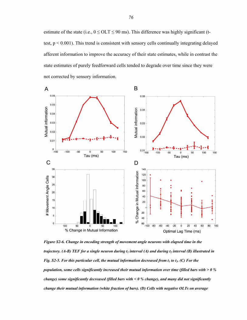
76
estimate of the state (i.e., 0 ≤ OLT ≤ 90 ms). This difference was highly significant (t-
test, p < 0.001). This trend is consistent with sensory cells continually integrating delayed
afferent information to improve the accuracy of their state estimates, while in contrast the
state estimates of purely feedforward cells tended to degrade over time since they were
not corrected by sensory information.
Figure S2-6. Change in encoding strength of movement angle neurons with elapsed time in the
trajectory. (A-B) TEF for a single neuron during t1 interval (A) and during t2 interval (B) illustrated in
Fig. S2-5. For this particular cell, the mutual information decreased from t1 to t2. (C) For the
population, some cells significantly increased their mutual information over time (filled bars with > 0 %
change) some significantly decreased (filled bars with < 0 % change), and many did not significantly
change their mutual information (white fraction of bars). (D) Cells with negative OLTs on average

77
tended to increase their information more with time, which is consistent with these cells relying upon
sensory information to improve their state estimate.
References
Andersen RA, Buneo CA (2002b) Intentional maps in posterior parietal cortex. Annual Review of Neuroscience 25:189-220.
Andersen RA, Essick GK, Siegel RM (1987) Neurons of area-7 activated by both visual-stimuli and oculomotor behavior. Exp Brain Res 67:316-322.
Ashe J, Georgopoulos AP (1994) Movement parameters and neural activity in motor cortex and area 5. Cereb Cortex 4:590-600.
Averbeck BB, Chafee MV, Crowe DA, Georgopoulos AP (2005) Parietal representation of hand velocity in a copy task. J Neurophysiol 93:508-518.
Bastian AJ (2006) Learning to predict the future: the cerebellum adapts feedforward movement control. Curr Opin Neurobiol 16:645-649.
Batista AP, Buneo CA, Snyder LH, Andersen RA (1999) Reach plans in eye-centered coordinates. Science 285:257-260.
Bessou P, Emonetde.F, Laporte Y (1965) Motor fibres innervating extrafusal and intrafusal muscle fibres in cat. J Physiol 180:649-&.
Blakemore SJ, Sirigu A (2003) Action prediction in the cerebellum and in the parietal lobe. Exp Brain Res 153:239-245.
Bradley DC, Maxwell M, Andersen RA, Banks MS, Shenoy KV (1996) Mechanisms of heading perception in primate visual cortex. Science 273:1544-1547.
Buneo CA, Jarvis MR, Batista AP, Andersen RA (2002) Direct visuomotor transformations for reaching. Nature 416:632-636.
Clower DM, West RA, Lynch JC, Strick PL (2001) The inferior parietal lobule is the target of output from the superior colliculus, hippocampus, and cerebellum. J Neurosci 21:6283-6291.
Cover TM, Thomas JA (1991) Elements of Information Theory. New York: John Wiley & Sons.
DeAngelis GC, Ghose GM, Ohzawa I, Freeman RD (1999) Functional micro-organization of primary visual cortex: Receptive field analysis of nearby neurons. J Neurosci 19:4046-4064.
Della-Maggiore V, Malfait N, Ostry DJ, Paus T (2004) Stimulation of the posterior parietal cortex interferes with arm trajectory adjustments during the learning of new dynamics. J Neurosci 24:9971-9976.
Desmurget M, Grafton S (2000) Forward modeling allows feedback control for fast reaching movements. Trends Cognit Sci 4:423-431.
Desmurget M, Epstein CM, Turner RS, Prablanc C, Alexander GE, Grafton ST (1999) Role of the posterior parietal cortex in updating reaching movements to a visual target. Nat Neurosci 2:563-567.
Fisher NI (1993) Statistical Analysis of Circular Data. Cambridge: Cambridge University Press.
78
Flanders M, Cordo PJ (1989) Kinesthetic and visual control of a bimanual task - Specification of direction and amplitude. J Neurosci 9:447-453.
Gallistel CR (1990) The Organization of Learning. Cambridge, MA: MIT Press. Gander W, Golub GH, Strebel R (1994) Least-squares fitting of circles and ellipses. Bit
34:558-578. Glickstein M (2000) How are visual areas of the brain connected to motor areas for the
sensory guidance of movement? Trends Neurosci 23:613-617. Goodwin GC, Sin KS (1984) Adaptive Filtering Prediction and Control. Englewood
Cliffs, NJ: Prentice-Hall. Haarmeier T, Thier P, Repnow M, Petersen D (1997) False perception of motion in a
patient who cannot compensate for eye movements. Nature 389:849-852. Haarmeier T, Bunjes F, Lindner A, Berret E, Thier P (2001) Optimizing visual motion
perception during eye movements. Neuron 32:527-535. Hatsopoulos NG, Xu QQ, Amit Y (2007) Encoding of movement fragments in the motor
cortex. J Neurosci 27:5105-5114. Houk JC, Rymer WZ, Crago PE (1981) Dependence of dynamic-response of spindle
receptors on muscle length and velocity. J Neurophysiol 46:143-166. Johnson PB, Ferraina S, Bianchi L, Caminiti R (1996) Cortical networks for visual
reaching: Physiological and anatomical organization of frontal and parietal lobe arm regions. Cereb Cortex 6:102-119.
Jones EG, Powell TP (1970) An anatomical study of converging sensory pathways within the cerebral cortex of the monkey. Brain 93:793-820.
Jordan MI, Rumelhart DE (1992) Forward models - supervised learning with a distal teacher. Cognit Sci 16:307-354.
Kalaska JF, Caminiti R, Georgopoulos AP (1983) Cortical mechanisms related to the direction of two-dimensional arm movements - relations in parietal area 5 and comparison with motor cortex. Exp Brain Res 51:247-260.
Kowalski N, Depireux DA, Shamma SA (1996) Analysis of dynamic spectra in ferret primary auditory cortex. 1. Characteristics of single-unit responses to moving ripple spectra. J Neurophysiol 76:3503-3523.
Matthews PBC (1972) Mammalian Muscle Receptors and Their Central Actions. London: Arnold.
Mazer JA, Vinje WE, McDermott J, Schiller PH, Gallant JL (2002) Spatial frequency and orientation tuning dynamics in area V1. Proc Natl Acad Sci USA 99:1645-1650.
Miall RC, Wolpert DM (1996) Forward models for physiological motor control. Neural Networks 9:1265-1279.
Miall RC, Weir DJ, Wolpert DM, Stein JF (1993) Is the Cerebellum a Smith Predictor. Journal of Motor Behavior 25:203-216.
Moran DW, Schwartz AB (1999) Motor cortical representation of speed and direction during reaching. J Neurophysiol 82:2676-2692.
Mountcastle VB, Lynch JC, Georgopoulos A, Sakata H, Acuna C (1975) Posterior parietal association cortex of monkey - command functions for operations within extrapersonal space. J Neurophysiol 38:871-908.
Newsome WT, Wurtz RH, Komatsu H (1988) Relation of cortical areas MT and MST to pursuit eye-movements. 2. Differentiation of retinal from extraretinal inputs. J Neurophysiol 60:604-620.

79
Paninski L, Fellows MR, Hatsopoulos NG, Donoghue JP (2004) Spatiotemporal tuning of motor cortical neurons for hand position and velocity. J Neurophysiol 91:515-532.
Pena JL, Konishi M (2001) Auditory spatial receptive fields created by multiplication. Science 292:249-252.
Petersen N, Christensen LOD, Morita H, Sinkjaer T, Nielsen J (1998) Evidence that a transcortical pathway contributes to stretch reflexes in the tibialis anterior muscle in man. J Physiol 512:267-276.
Pisella L, Grea H, Tilikete C, Vighetto A, Desmurget M, Rode G, Boisson D, Rossetti Y (2000) An 'automatic pilot' for the hand in human posterior parietal cortex: toward reinterpreting optic ataxia. Nat Neurosci 3:729-736.
Prochazka A, Gorassini M (1998) Models of ensemble firing of muscle spindle afferents recorded during normal locomotion in cats. J Physiol 507:277-291.
Raiguel SE, Xiao DK, Marcar VL, Orban GA (1999) Response latency of macaque area MT/V5 neurons and its relationship to stimulus parameters. Journal of Neurophysiology 82:1944-1956.
Sarndal CE (1974) A comparative study of association measures. Psychometrika 39:165-187.
Schwartz AB, Kettner RE, Georgopoulos AP (1988) Primate motor cortex and free arm movements to visual targets in 3-dimensional space. 1. Relations between single cell discharge and direction of movement. J Neurosci 8:2913-2927.
Snyder LH, Batista AP, Andersen RA (1997) Coding of intention in the posterior parietal cortex. Nature 386:167-170.
Srinivasan L, Brown EN (2007) A state-space framework for movement control to dynamic goals through brain-driven interfaces. IEEE Trans Biomed Eng 54:526-535.
von Helmoltz H (1866) Handbook of Physiological Optics (3rd ed.). New York: Dover Publications.
Von Holst E, Mittelstaedt H (1950) Das reafferenzprinzip. Die Naturwissenschaften 37:464-476.
Wang XL, Zhang MS, Cohen IS, Goldberg ME (2007) The proprioceptive representation of eye position in monkey primary somatosensory cortex. Nat Neurosci 10:640-646.
Wolpert DM, Ghahramani Z, Jordan MI (1995) An internal model for sensorimotor integration. Science 269:1880-1882.
Wolpert DM, Goodbody SJ, Husain M (1998a) Maintaining internal representations the role of the human superior parietal lobe. Nat Neurosci 1:529-533.
Wolpert DM, Miall RC, Kawato M (1998b) Internal models in the cerebellum. Trends Cognit Sci 2:338-347.
Wu W, Hatsopoulos N (2006) Evidence against a single coordinate system representation in the motor cortex. Exp Brain Res 175:197-210.

80
Chapter 3
DECODING TRAJECTORIES FROM PPC ENSEMBLES
3.1 Summary
High-level cognitive signals in the posterior parietal cortex (PPC) have previously been
used to decode the intended endpoint of a reach, providing the first evidence that PPC
can be used for direct control of a neural prosthesis (S. Musallam et al., 2004). Here we
expand on this work by showing that PPC neural activity can be harnessed to estimate
not only the endpoint but also to continuously control the trajectory of an end effector.
Specifically, we trained two monkeys to use a joystick to guide a cursor on a computer
screen to peripheral target locations while maintaining central ocular fixation. We found
that we could accurately reconstruct the trajectory of the cursor using a relatively small
ensemble of simultaneously recorded PPC neurons. Using a goal-based Kalman filter
that incorporates target information into the state-space model, we showed that the
decoded estimate of cursor position could be significantly improved. In addition, we
demonstrated that by optimizing the depth of multiple electrodes based upon
electrophysiological feedback of the recording quality, decoding efficiency (i.e., the R2
per channel) of the PPC ensemble was markedly improved, compared to traditional
fixed-depth array recordings.
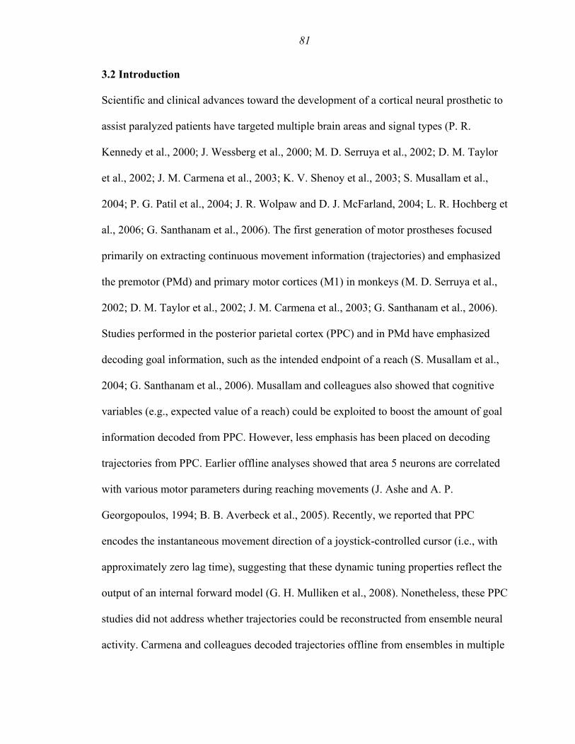
81
3.2 Introduction
Scientific and clinical advances toward the development of a cortical neural prosthetic to
assist paralyzed patients have targeted multiple brain areas and signal types (P. R.
Kennedy et al., 2000; J. Wessberg et al., 2000; M. D. Serruya et al., 2002; D. M. Taylor
et al., 2002; J. M. Carmena et al., 2003; K. V. Shenoy et al., 2003; S. Musallam et al.,
2004; P. G. Patil et al., 2004; J. R. Wolpaw and D. J. McFarland, 2004; L. R. Hochberg et
al., 2006; G. Santhanam et al., 2006). The first generation of motor prostheses focused
primarily on extracting continuous movement information (trajectories) and emphasized
the premotor (PMd) and primary motor cortices (M1) in monkeys (M. D. Serruya et al.,
2002; D. M. Taylor et al., 2002; J. M. Carmena et al., 2003; G. Santhanam et al., 2006).
Studies performed in the posterior parietal cortex (PPC) and in PMd have emphasized
decoding goal information, such as the intended endpoint of a reach (S. Musallam et al.,
2004; G. Santhanam et al., 2006). Musallam and colleagues also showed that cognitive
variables (e.g., expected value of a reach) could be exploited to boost the amount of goal
information decoded from PPC. However, less emphasis has been placed on decoding
trajectories from PPC. Earlier offline analyses showed that area 5 neurons are correlated
with various motor parameters during reaching movements (J. Ashe and A. P.
Georgopoulos, 1994; B. B. Averbeck et al., 2005). Recently, we reported that PPC
encodes the instantaneous movement direction of a joystick-controlled cursor (i.e., with
approximately zero lag time), suggesting that these dynamic tuning properties reflect the
output of an internal forward model (G. H. Mulliken et al., 2008). Nonetheless, these PPC
studies did not address whether trajectories could be reconstructed from ensemble neural
activity. Carmena and colleagues decoded trajectories offline from ensembles in multiple

82
brain areas including PPC, M1, PMd and primary somatosensory cortex (S1) (J.
Wessberg et al., 2000; J. M. Carmena et al., 2003). However, they reported relatively
poor offline reconstruction performance for their PPC sample, an unexpected result based
upon previous encoding findings.
Therefore, the extent to which PPC can be used to decode trajectories offline remains
uncertain. Here we show that trajectories can be reliably reconstructed offline using
relatively small numbers of simultaneously recorded PPC neurons. We also show that
goal-based, state-space decoding methods, as well as adjustable-depth multi-electrode
array (AMEA) recording techniques, can be advantageous for a prosthesis targeting PPC.
Finally, we show that when recording from ensembles using an adjustable-depth multi-
electrode array (AMEA), in which the single-cell isolation quality of each electrode can
be optimized, we were able to decode trajectory information more efficiently from PPC,
requiring fewer electrodes on average.
3.3 Materials and methods
3.3.1 Animal preparation
Two male rhesus monkeys (Macacca mulatta; 6–9 kg) were used in this study. All
experiments were performed in compliance with the guidelines of the Caltech
Institutional Animal Care and Use Committee and the National Institutes of Health Guide
for the Care and Use of Laboratory Animals.

83
3.3.2 Neurophysiological recording
We recorded multi-channel neural activity from two monkeys in the medial bank of the
intraparietal sulcus (IPS) and area 5. We implanted two 32-channel microwire arrays (64
electrodes) in one monkey (1st array 6-8 mm deep in IPS, 2nd array 1-2 mm deep in area
5). Chronically implanted array placements were planned using magnetic resonance
imaging (MRI) and carried out using image-guided surgical techniques to accurately
target the desired anatomical location and to minimize the extent of the craniotomy
(Omnisight Image-guided Surgery System, Radionics, Burlington, MA). In a second
monkey we performed acute chamber recordings using a 6-channel microdrive (NAN
Electrode Drive, Plexon, Dallas, TX). The placement of the recording chamber was
verified using MRI, with the chamber centered at 5 mm posterior, 6 mm lateral in
stereotaxic coordinates. For the remainder of this report, we will refer to a chronic
microwire array as a fixed-depth multi-electrode array (FMEA) and the microdrive as an
adjustable-depth multi-electrode array (AMEA). Spike-sorting was performed online
using a Plexon multi-channel data acquisition system and later confirmed with offline
analysis using the Plexon Offline Sorter. Using the AMEA technique, we were able to
maintain single-unit isolations of several neurons for approximately 1-2 hours. Note that
we did not specify that isolated neurons be tuned to a particular parameter measured in
our task, but instead only required that each neuron have a minimum baseline firing rate
(> 2 Hz). Once single-unit isolations were established manually, isolations were
maintained using an autonomous electrode positioning algorithm (SpikeTrack), which
independently adjusted the depth of each of the six electrodes in order to continuously
optimize extracellular isolation quality (J. G. Cham et al., 2005; Z. Nenadic and J. W.

84
Burdick, 2005; E. A. Branchaud et al., 2006). It should be noted that all neural units
reported using the AMEA technique were well-isolated single-units, while neural units
recorded using the FMEA technique consisted of a combination of single and multi-unit
activity.
3.3.3 Experimental design
Monkeys were trained to perform a 2D center-out joystick (J50 2-axis joystick, ETI
Systems, Fort Worth, TX) reaction task, in which they were required to guide a cursor on
a computer screen to illuminated peripheral targets. After several weeks of training, the
monkeys were highly skilled at the task and were performing regularly above 90%
success rate.
The 2D center-out joystick task is illustrated in Figure 3-1A. The monkeys sat 45 cm in
front of an LCD monitor. Eye position was monitored with an infrared oculometer.
Monkeys initiated a trial by moving a white cursor (0.9 deg) into a central green target
circle (4.4 deg) and then fixated a concentric, central red circle (1.6 deg). After 350 ms,
the target jumped to 1 of 8 (or 12) random peripheral locations (11-14.7 deg). The
monkeys then guided the cursor smoothly into the peripheral target zone while
maintaining central fixation. Once the cursor was held within 2.2 deg of the target center
for 350 ms, the monkeys were rewarded with a drop of juice. If fixation was broken
during the movement, the trial was aborted. Monkeys were required to fixate centrally
during the entire trajectory in order to maintain a constant visual reference frame. Earlier
studies have shown that parietal reach region (PRR) encodes visual targets for reaching in
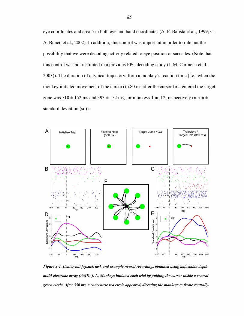
85
eye coordinates and area 5 in both eye and hand coordinates (A. P. Batista et al., 1999; C.
A. Buneo et al., 2002). In addition, this control was important in order to rule out the
possibility that we were decoding activity related to eye position or saccades. (Note that
this control was not instituted in a previous PPC decoding study (J. M. Carmena et al.,
2003)). The duration of a typical trajectory, from a monkey’s reaction time (i.e., when the
monkey initiated movement of the cursor) to 80 ms after the cursor first entered the target
zone was 510 ± 152 ms and 393 ± 152 ms, for monkeys 1 and 2, respectively (mean ±
standard deviation (sd)).
Figure 3-1. Center-out joystick task and example neural recordings obtained using adjustable-depth
multi-electrode array (AMEA). A, Monkeys initiated each trial by guiding the cursor inside a central
green circle. After 350 ms, a concentric red circle appeared, directing the monkeys to fixate centrally.

86
The target was randomly jumped to 1 of 8 possible targets, at which point the monkey initiated a
trajectory to the peripheral target location. Monkeys held the cursor inside the target for at least 350 ms
(100 ms for brain control – see Chapter 4) before receiving a juice reward. Raster plots show responses
of 5 simultaneously recorded neurons during trajectories to two different target locations, leftward (180
deg) (B) and rightward (0 deg) (C). Neural activity is aligned to the time of movement initiation (dashed
vertical line) and is plotted up to 80 ms after the cursor entered the target zone. Standardized firing rate
time courses for all 5 neurons (sorted by color) are plotted below their respective raster plots for both
leftward (D) and rightward (E) target conditions. Note the spatial tuning present for two targets in this
ensemble of 5 neurons. Smoothed (Gaussian kernel, sd = 20 ms) traces were generated for illustrative
purposes here, while binned standardized firing rates were in fact used to train decoding algorithms (see
Methods). F, Example trajectories made by monkey 1 for all 8 targets. The dashed green circle is the
starting location of the target and is not visible once the target has been jumped to the periphery. Dots
represent cursor position sampled at 15 ms intervals along the trajectory.
3.3.4 Offline algorithm construction
We sought to construct a decoding model that optimally estimated behavioral parameters
from the firing rates of simultaneously recorded PPC neurons (e.g., minimized the mean
squared reconstruction error, MSE). To further illustrate this situation, we have plotted
simultaneously recorded spike trains from 5 neurons in the raster plots of Figure 3-1B-C,
which were collected during 10 trials made to both leftward and rightward targets. Neural
activity is aligned to the reaction time and is plotted up to 80 ms after the cursor entered
the target zone. Below each set of raster plots are the trial-averaged, standardized firing
rate time courses associated with each of these two target directions. The instantaneous
firing rate of a neuron was standardized by first subtracting the neuron’s mean firing rate
and then dividing by its standard deviation. Using an ensemble of standardized firing

87
rates along with concurrently recorded behavioral data from the joystick training
segment, we constructed a mathematical decoding model to attempt to reconstruct the
monkeys’ trajectories offline. To accomplish this, we tested two standard linear
estimation algorithms: ridge regression and a modified Kalman filter (R. E. Kalman,
1960; A. E. Hoerl and R. W. Kennard, 1970). 5-fold cross-validation was used to assess
performance and to perform model selection. Specifically, all trials from a joystick
training segment were shuffled and then divided into five equal parts. 4/5 parts were used
to train the model and 1/5 parts was used to validate the model. Thus, the trained model
was validated five times to obtain an average performance, with each of the five parts
serving as the validation set one time.
3.3.5 Ridge regression
We first constructed a linear model of the instantaneous 2D cursor position (or velocity,
acceleration, target position) at some time, x(t), as a function of the standardized firing
rates of N simultaneously recorded neural units. Firing rates were computed for non-
overlapping 80 ms bins, and effectively represented the mean firing rate measured at the
middle of each bin. Each sample of the behavioral state vector, x(t) , was modeled as a
function of the vector of ensemble firing rates measured for three preceding time bins
(i.e., lag times), centered at , which effectively
represented the temporal evolution of the causal ensemble activity prior to each
behavioral state measurement. To simplify our notation, we will refer to discretized time
steps (k) for the remainder of this report, where x(k) denotes the instantaneous behavioral
measurement and r(k) denotes the average binned firing rate of the ensemble 40 ms in the
)}), r(t-), r(t-{r(t- ms 40ms 120ms 200

88
past, r(k-1) denotes the mean firing rate 120 ms in the past, etc. We tried a variety of bin
sizes and number of lag time steps and found that these values provided the best
performance over multiple sessions. During a given trial, spiking activity was sampled
beginning from 240 ms before the monkeys’ reaction time up to 80 ms after the cursor
first entered the target zone. An estimate of the 2D cursor position (or velocity, etc.),
, was constructed as a linear combination of the ensemble of firing rates, r, sampled
at multiple lag time steps according to
)(ˆ kx
, (1) ( ) )(,)(ˆ2
0,0 ikjikrkx
i
N
jji −+−+= ∑∑
=
εββ
where ε represents the observational error. The MSE of the estimate, , can generally
be decomposed into two parts, a bias and a variance component, which can vary in size
depending upon the method used to obtain β, thereby producing an important trade-off to
be considered during model selection (S. Geman et al., 1992). The well-known least
squares solution for β, which can be obtained in a single step, yields the minimum
variance, unbiased estimator. However, a zero-bias estimator often suffers from high
MSE due to a large variance component of the error. Often, it is beneficial during model
selection to slacken the constraint on the bias in order to further reduce the variance
component of the error. In particular, this is beneficial when confronted with a high-
dimensional input space in which many neural signals may be correlated (e.g., over-
lapping receptive fields or auto-correlated firing rate inputs from different lag time steps),
which may result in estimators that exhibit large variability over a number of different
training sets. Ridge regression is a method that can optimize the bias-variance tradeoff by
penalizing the average size of the coefficients in order to reduce the variance component
)(ˆ kx
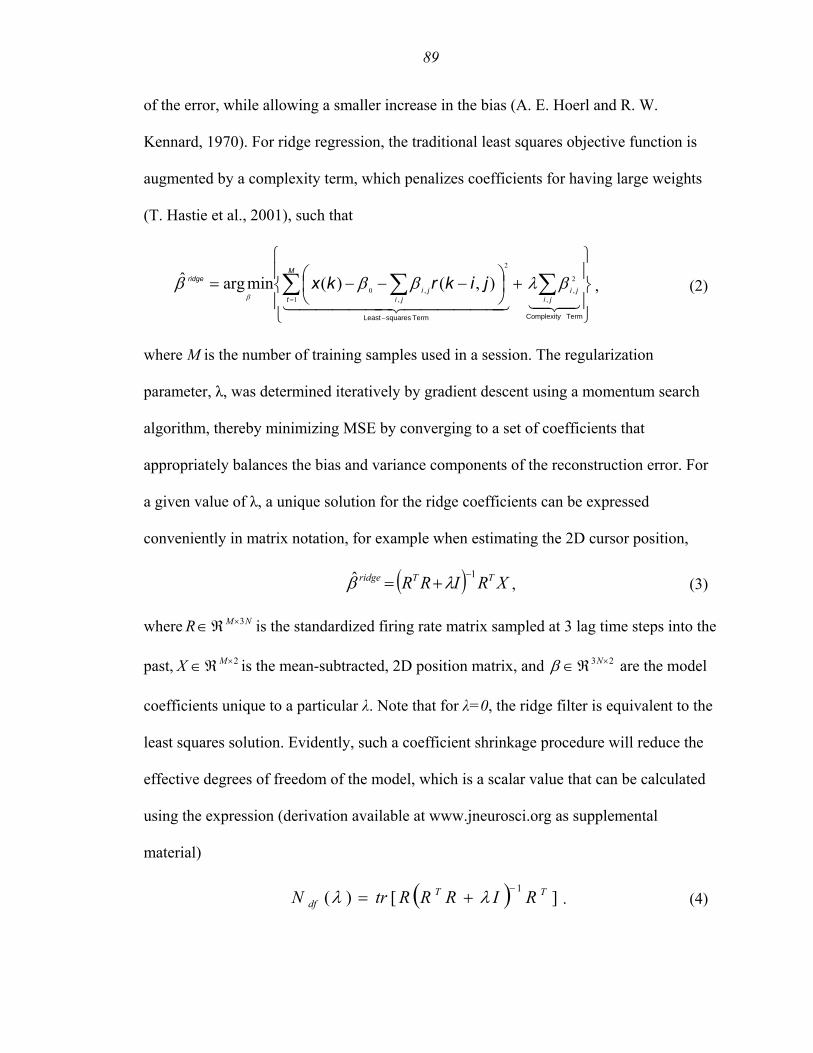
89
of the error, while allowing a smaller increase in the bias (A. E. Hoerl and R. W.
Kennard, 1970). For ridge regression, the traditional least squares objective function is
augmented by a complexity term, which penalizes coefficients for having large weights
(T. Hastie et al., 2001), such that
, (2) ⎪⎭
⎪⎬
⎫
⎪⎩
⎪⎨
⎧
+⎟⎠⎞
⎜⎝⎛ −−−= ∑∑ ∑
−
= 43421444444 3444444 21Term ComplexityTerm squaresLeast
jiji
M
t jiji
ridge jikrkx,
2
,1
2
,,0 ),()(minargˆ βλβββ
β
where M is the number of training samples used in a session. The regularization
parameter, λ, was determined iteratively by gradient descent using a momentum search
algorithm, thereby minimizing MSE by converging to a set of coefficients that
appropriately balances the bias and variance components of the reconstruction error. For
a given value of λ, a unique solution for the ridge coefficients can be expressed
conveniently in matrix notation, for example when estimating the 2D cursor position,
( ) XRIRR TTridge 1ˆ −+= λβ , (3)
where is the standardized firing rate matrix sampled at 3 lag time steps into the
past, is the mean-subtracted, 2D position matrix, and are the model
coefficients unique to a particular λ. Note that for λ=0, the ridge filter is equivalent to the
least squares solution. Evidently, such a coefficient shrinkage procedure will reduce the
effective degrees of freedom of the model, which is a scalar value that can be calculated
using the expression (derivation available at www.jneurosci.org as supplemental
material)
NMR 3×ℜ∈
2×ℜ∈ MX 23 ×ℜ∈ Nβ
( ) ][)( 1 TTdf RIRRRtrN −
+= λλ . (4)
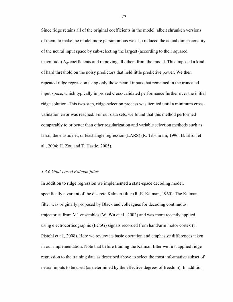
90
Since ridge retains all of the original coefficients in the model, albeit shrunken versions
of them, to make the model more parsimonious we also reduced the actual dimensionality
of the neural input space by sub-selecting the largest (according to their squared
magnitude) Ndf coefficients and removing all others from the model. This imposed a kind
of hard threshold on the noisy predictors that held little predictive power. We then
repeated ridge regression using only those neural inputs that remained in the truncated
input space, which typically improved cross-validated performance further over the initial
ridge solution. This two-step, ridge-selection process was iterated until a minimum cross-
validation error was reached. For our data sets, we found that this method performed
comparably to or better than other regularization and variable selection methods such as
lasso, the elastic net, or least angle regression (LARS) (R. Tibshirani, 1996; B. Efron et
al., 2004; H. Zou and T. Hastie, 2005).
3.3.6 Goal-based Kalman filter
In addition to ridge regression we implemented a state-space decoding model,
specifically a variant of the discrete Kalman filter (R. E. Kalman, 1960). The Kalman
filter was originally proposed by Black and colleagues for decoding continuous
trajectories from M1 ensembles (W. Wu et al., 2002) and was more recently applied
using electrocorticographic (ECoG) signals recorded from hand/arm motor cortex (T.
Pistohl et al., 2008). Here we review its basic operation and emphasize differences taken
in our implementation. Note that before training the Kalman filter we first applied ridge
regression to the training data as described above to select the most informative subset of
neural inputs to be used (as determined by the effective degrees of freedom). In addition

91
to standard kinematic state variables (i.e., position (p), velocity (v), acceleration (a)) used
in the above mentioned M1 studies, we incorporated goal information into the state-space
representation by augmenting the kinematic state vector with the static target position, T,
that is
. (5) T
yxyxyxyxk TTaavvppx ],,,,,,,[=
To avoid confusion with the standard Kalman filter, we will refer to our model as the
goal-based Kalman filter (G-Kalman filter) for the remainder of this report.
Unlike the feedforward ridge filter, the G-Kalman filter operates in a recursive manner
using two governing equations instead of one: an observation equation that models the
firing rates (observation) as a function of the state of the cursor, xk, and a process
equation that operates in a Markov fashion to propagate the state of the cursor forward in
time as a function of only the most recent state, xk-1 (G. Welch and G. Bishop, 2006).
Therefore, firing rates are not binned in multiple lag time steps prior to the measured state
xk, but instead reflect the firing rate of a single 80 ms bin just before (i.e., t-40 ms) the
measured state of the cursor. The G-Kalman filter assumes that these two models are
linear stochastic functions, which operate under the condition of additive Gaussian white
noise according to
111 −−− ++= kkkkk wBuxAx
kkkk xHr
, (process equation) (6)
ν+= (observation equation). (7)
The control term, u, is assumed to be unidentified and is therefore set to zero in our
model, excluding B from the process model. Following the approach of Wu and
colleagues, we made the simplifying assumption that the process noise ( ), 18×ℜ∈w

92
observation noise ( ), transition matrix ( ) and the observation matrix
( ) were fixed in time (W. Wu et al., 2002). Simplifying,
18×ℜ∈v
kx =
kr =
66×ℜ∈kin
26×ℜ∈C
88×ℜ∈A
(~)( Nwp
Nv ,0(~)(
⎥⎦
⎤
IC
kx
8×ℜ∈ NH
, (8) 881 ),,0 where, x
k QQwAx ℜ∈+−
, (9) NxNk VVpHx ℜ∈+ ), where,ν
where A and H were solved using least squares regression and Q and V are the process
and observation noise covariance matrices, respectively. Note that the transition matrix,
A, took the form
, (10) ⎢⎣
⎡=
AA
kin
0
where I is the 2 x 2 identity matrix, indicating that the target was fixed in time during the
trial. The estimate of the kinematic state of the cursor, , was
therefore a linear combination of the previous kinematic state, which was weighted by the
transition matrix , and the estimated target position, which was weighted by
the linear operator . That is, C biased the estimate of the kinematic state to be
spatially constrained by the target position, which was inferred from the neural
observation in Equation 9.
Tyxyxyx aavvpp ],,,,,[=
A
To estimate the state of the cursor at each time step k, the output of the process model,
(i.e., a priori estimate), was linearly combined with the difference between the output of
the observation model and the actual neural measurement (i.e., the neural innovation)
using an optimal scaling factor, the Kalman gain, Kk, to produce an a posterior estimate
of the state of the cursor,
−kx̂

93
( ) ˆˆˆ −− −+= kkkkk xHrKxx . (11)
This standard two-step discrete estimation process, consisting of an a priori time update
and a posterior measurement update, was iterated recursively to generate an estimate of
the state of the cursor at each time step in the trajectory (detailed description of this
process available at www.jneurosci.org as supplemental material). The initial position of
the cursor was assumed to be known, but the initial velocity, acceleration, and target
position were set to the expected value of their respective training distributions.
Similarly, the initial variance of the position was set to zero, reflecting no uncertainty
about the starting location of the cursor, while the variance for velocity, acceleration, and
target position were derived from their training set distributions:
[ ]][][][00 Txxxx ΕΕΕ= &&&
⎢⎢⎢⎢
⎣
⎡
=
000][00
0][0000
0 xVarxVar
P&&
&
(12)
, (13)
⎥⎥⎥⎥
⎦
⎤
][000
TVar
where E is the expected value operator.
We assessed the decoding performance of the G-Kalman filter for the entire duration of
the trajectory, though the G-Kalman filter typically converged to a steady-state value
(i.e., Kalman gain and error covariance decreased exponentially to asymptote) < 1s after
movement onset (further information available at www.jneurosci.org as supplemental
material).

94
3.3.7 Model assessment
We quantified the offline reconstruction performance of each decoding algorithm using a
single statistical criterion, the coefficient of determination, or R2. R2 values for X and Y
directions were averaged to give a single R2 value for position, velocity etc.
We also constructed neuron-dropping curves for each session to quantify how well
trajectories could be reconstructed using PPC ensembles of different sizes. To assess the
performance of a particular ensemble size, q, we randomly selected and removed Ndf - q
neural units from the original ensemble, which contained Ndf total neural units. Next, we
performed 5-fold cross-validation using the remaining q neural units to obtain an R2
value, then replaced them, and repeated this procedure 50 times to obtain an average R2
for each ensemble size, q. Note that an equal number of randomly selected trials were
used from each session (300 trials); however we typically did not observe a significant
improvement in performance after including much more than 100 trials.
We computed model fits for the resultant neuron-dropping curves so that they could be
extrapolated to theoretical, larger ensemble sizes, allowing us estimate the average R2
performance for an arbitrary ensemble size. An exponential recovery function was fit to
the data according to
, (14) zqeR /2 1 −−=
where q was the ensemble size used and z was a fitted constant. For all FMEA and
AMEA plots, the quality of fit obtained using these models was very good (average R2 >
0.98).

95
3.3.8 Neural unit waveform analysis
We quantified the signal to noise (SNR) ratio of neural unit waveforms according to the
method described by Suner and colleagues (S. Suner et al., 2005). Using this method,
SNR was calculated by dividing the average peak-to-peak amplitude for an aligned spike
waveform by a noise term. The noise term was equal to the twice the sd of the residuals
that remained after subtracting the mean spike waveform from all waveform samples for
a particular neural unit. The minimum threshold SNR required for multi-unit
classification was 2. Single-units were identified using offline sorting, and always had
inter-spike intervals above 2 ms and typically had SNR values above 4 when using this
method.
3.4 Results
3.4.1 Offline decoding
Our objective was to construct a decoding model that estimated task-related behavioral
parameters (e.g., position, velocity, acceleration, target position) at multiple time steps in
a trajectory from parallel observations of PPC neural activity. Training sets used for 5-
fold cross validation were constructed from approximately 300 joystick trials per session.
We analyzed a total of 20 different recording sessions offline and found that we could
reconstruct joystick trajectories with very good accuracy using ensemble activity from
PPC, accounting for more than 70% of the variance in the cursor position during a single
session (R2 = 0.71). 10 recording sessions were performed using FMEAs implanted in
one monkey, yielding recordings which were comprised of a combination of single and

96
multi-units (7.8 ± 5.2 single-units, 107 ± 27 multi-units, Ndf = 65 ± 27 neural units, mean
± sd). An additional set of 10 sessions was collected using AMEA recordings from a
second monkey, all 10 of which contained exactly 5 simultaneously recorded single-units
(no multi-unit activity was included in the AMEA ensembles). Note that offline decoding
analyses using FMEA data were performed for sessions recorded prior to the monkey
ever having ever experienced brain control (see Chapter 4). Therefore, all offline analyses
reflected our ability to decode from PPC ensembles prior to the development of any
learning effects that occurred as a result of brain control.
3.4.2 Position decoding performance: model comparisons
We evaluated the performances of several decoding algorithms, including least squares,
ridge regression, a standard Kalman filter and the G-Kalman filter. In general, when
estimating the position of the cursor, we found that the G-Kalman filter out-performed
the other three decoding algorithms, followed next by the Kalman filter, then the ridge
filter and finally the least squares model (Fig. 3-2A-B). For instance, for FMEA
recordings, we found that ridge regression significantly improved the decoding
performance when compared to the least squares model (p = 0.002, two-sided sign test),
on average resulting in a median improvement of 71% (first quartile (Q1) = 34%, third
quartile (Q3) = 109%). However, as expected, we did not observe a significant change (p
= 0.50, two-sided sign test) when using ridge for AMEA-recorded activity (0% median
improvement, Q1 = 0, Q3 = 1). This discrepancy likely reflects the benefit of using ridge
regression and subselection for high-dimensional input spaces (i.e., FMEA) that exhibited
multicollinearity among neural inputs and/or contained little or no tuned activity on some

97
channels. Consistent with this reasoning, we observed that the complexity parameter, λ,
which was used to shrink the average size of the model coefficients, was significantly
larger for FMEA data sets than for AMEA data sets (p < 0.007, Wilcoxon rank sum test).
In addition, we found that for both AMEA and FMEA sessions, the standard Kalman
filter significantly outperformed the ridge filter (p = 0.001, two-sided sign test)) (53%
improvement (Q1 = 34, Q3 = 97)). This finding is in agreement with evidence from
another study that showed that the Kalman filter outperformed the least squares filter
when decoding trajectories from M1 ensembles (W. Wu et al., 2002), and likely reflects
the benefit of exploiting velocity information (that is encoded by some PPC neurons and
inferred via Equation 9) to dynamically estimate the changing position of the cursor (via
Equation 8).
Figure 3-2. Offline decoding performance for trajectory reconstructions. A, Single session R2 values for
position estimation using the AMEA and fixed-depth multi-electrode array (FMEA) techniques.
Performances of several models are compared in the bar chart, including least squares (LS), ridge
regression, the Kalman filter, and the goal-based Kalman Filter (G-Kalman)). B, Average R2
performances for 10 FMEA sessions and 10 AMEA sessions for each of the four models. Higher
decoding performance for FMEA recordings relative to AMEA recordings when using Kalman filter

98
decoding models can likely be explained by the existence of stronger velocity-tuned neurons present for
FMEA recordings.
Previous neurophysiological studies have established that PPC neurons encode a reach
plan toward an intended goal location in eye-centered coordinates (L. H. Snyder et al.,
1997; R. A. Andersen and C. A. Buneo, 2002; A. Gail and R. A. Andersen, 2006; R. Q.
Quiroga et al., 2006). In addition, other studies have shown that PPC maintains a strong
representation of the target location even during continuous control of a movement (J.
Ashe and A. P. Georgopoulos, 1994; G. H. Mulliken et al., 2008). Therefore we tested
whether information about the static target location could be extracted from PPC and
used to improve the decoding accuracy of cursor position in our task. We found that the
decoding performance was significantly improved when using the G-Kalman filter (p <
1e-3, two-sided sign test), on average by 15% (median, Q1 = 9, Q3 = 24)), relative to the
standard Kalman filter. This result demonstrates that significant goal information could
be extracted from PPC, which was independent from the kinematic state of the cursor.
Furthermore, this information was harnessed by the G-Kalman filter to consistently
improve the estimate of the dynamic position of the cursor. It would be interesting to test
the extent to which decoding performance can be improved if more accurate target
information can be extracted from PPC (e.g., stronger target representations have
generally been found in deeper regions of the IPS (G. H. Mulliken et al., 2008)).
Therefore, we simulated the hypothetical situation in which the target position could be
inferred perfectly from the neural activity by assuming that the initial target position was
given and thereby fixed throughout the trial. This ideal case would result in an
approximately twofold average increase in performance (98% median increase, Q1 = 52,
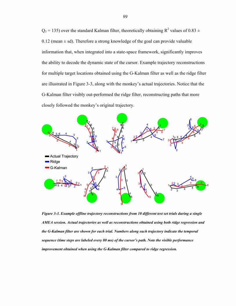
99
Q3 = 135) over the standard Kalman filter, theoretically obtaining R2 values of 0.83 ±
0.12 (mean ± sd). Therefore a strong knowledge of the goal can provide valuable
information that, when integrated into a state-space framework, significantly improves
the ability to decode the dynamic state of the cursor. Example trajectory reconstructions
for multiple target locations obtained using the G-Kalman filter as well as the ridge filter
are illustrated in Figure 3-3, along with the monkey’s actual trajectories. Notice that the
G-Kalman filter visibly out-performed the ridge filter, reconstructing paths that more
closely followed the monkey’s original trajectory.
Figure 3-3. Example offline trajectory reconstructions from 10 different test set trials during a single
AMEA session. Actual trajectories as well as reconstructions obtained using both ridge regression and
the G-Kalman filter are shown for each trial. Numbers along each trajectory indicate the temporal
sequence (time steps are labeled every 80 ms) of the cursor’s path. Note the visible performance
improvement obtained when using the G-Kalman filter compared to ridge regression.
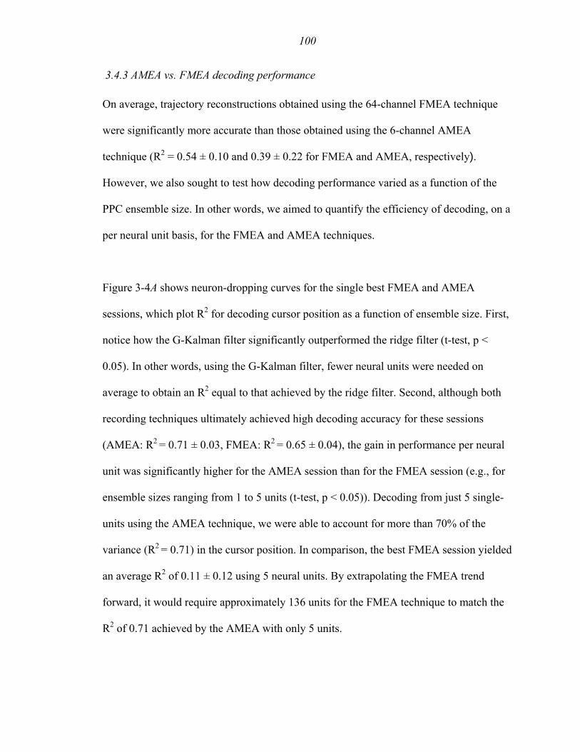
100
3.4.3 AMEA vs. FMEA decoding performance
On average, trajectory reconstructions obtained using the 64-channel FMEA technique
were significantly more accurate than those obtained using the 6-channel AMEA
technique (R2 = 0.54 ± 0.10 and 0.39 ± 0.22 for FMEA and AMEA, respectively).
However, we also sought to test how decoding performance varied as a function of the
PPC ensemble size. In other words, we aimed to quantify the efficiency of decoding, on a
per neural unit basis, for the FMEA and AMEA techniques.
Figure 3-4A shows neuron-dropping curves for the single best FMEA and AMEA
sessions, which plot R2 for decoding cursor position as a function of ensemble size. First,
notice how the G-Kalman filter significantly outperformed the ridge filter (t-test, p <
0.05). In other words, using the G-Kalman filter, fewer neural units were needed on
average to obtain an R2 equal to that achieved by the ridge filter. Second, although both
recording techniques ultimately achieved high decoding accuracy for these sessions
(AMEA: R2 = 0.71 ± 0.03, FMEA: R2 = 0.65 ± 0.04), the gain in performance per neural
unit was significantly higher for the AMEA session than for the FMEA session (e.g., for
ensemble sizes ranging from 1 to 5 units (t-test, p < 0.05)). Decoding from just 5 single-
units using the AMEA technique, we were able to account for more than 70% of the
variance (R2 = 0.71) in the cursor position. In comparison, the best FMEA session yielded
an average R2 of 0.11 ± 0.12 using 5 neural units. By extrapolating the FMEA trend
forward, it would require approximately 136 units for the FMEA technique to match the
R2 of 0.71 achieved by the AMEA with only 5 units.

101
Figure 3-4. Neuron-dropping curves comparing AMEA and FMEA decoding efficiencies. A, Recordings
from a single session showed significant decoding efficiency (R2/unit) advantages when using the AMEA
technique compared to the FMEA approach. (Note this particular FMEA session contained 115 neural
units.) B, These decoding efficiency differences were consistently observed when averaged across
multiple sessions (10 AMEA, 10 FMEA sessions). It is important to note that extrapolations made for
AMEA neuron-dropping curves were performed only for illustrative purposes and should not be
considered as accurate estimates of R2 for ensemble sizes much larger than 5 neurons. Future AMEA
studies will be necessary to collect data to confirm or deny such speculative AMEA projections. In
contrast, meaningful conclusions can be deduced from extrapolated data for FMEA neuron-dropping
curves since these projections are considerably more conservative.
To verify that these single-session trends were representative of the decoding efficiency
differences between AMEA and FMEA techniques in general, we averaged neuron
dropping curves from 10 AMEA sessions and 10 FMEA sessions. Note that when
averaging performances across all 10 FMEA sessions, the maximum possible number of
neural units considered was constrained by an upper limit of 46, the smallest ensemble
size, Ndf, of any of the 10 FMEA sessions we considered (i.e., in particular, the 46 neural
units that contained the largest predictive power for a given session). As expected,
102
session-averaged neuron-dropping curves were shifted downward from the single best
session curves due to variation in decoding performance across multiple sessions (Figure
3-4B). Nonetheless, trends analogous to those reported for single best sessions in Figure
3-2A were preserved after averaging across sessions. In particular, we observed
significant differences in R2 performance between AMEA and FMEA groups for all
ensemble sizes ranging from 1 to 5 neural units (t-test, p<0.05). On average, when
decoding with 5 neural units, an R2 of 0.35 ± 0.24 was achieved using the AMEA
technique while an R2 of 0.10 ± 0.13 was obtained using the FMEA approach. By
applying a model fit to the FMEA curve, we projected that it would require
approximately 27 neural units to reach an R2 of 0.71, which the AMEA approach
achieved using 5 just neural units. These data show that the AMEA technique was
substantially more efficient at extracting information from neural ensembles in PPC than
the FMEA technique. In addition, we performed a more quantitative analysis of decoding
efficiency by fitting Equation 15 to the FMEA and AMEA neuron dropping curves. The
model fit yielded a decoding efficiency constant, z, which was z = 11.7 and z = 64.1, for
the AMEA and FMEA traces, respectively. This result suggests that, on average, position
information could be decoded approximately 6 times more efficiently from the AMEA
population than from the FMEA implant.
3.4.4 Reconstruction of behavioral and task parameters
We also tested how well the G-Kalman filter could estimate several other behavioral and
task parameters. Figure 3-5 illustrates a 4-second time course of position, velocity, and
acceleration of the cursor as well as the target position, which were constructed by

103
concatenating segments from 9 test trials randomly selected from a single session.
Superimposed onto the plot are the estimated values of these parameters, which were
generated using the G-Kalman filter. Notice that the estimated values of position, velocity
and target position followed their corresponding experimental values reasonably closely.
As expected, estimation of acceleration from PPC activity was contrastingly less reliable,
since physical measurements of acceleration tend to be comparably noisy due to the
higher-frequency characteristic of acceleration. For this session, using the G-Kalman
filter we found that PPC activity was capable of yielding R2 estimation accuracies of up
to 0.71, 0.57, 0.25 and 0.64, for position, velocity, acceleration, and target position,
respectively. On average, across all FMEA sessions, when using the G-Kalman filter we
found that R2position = 0.54 ± 0.10, R2
velocity = 0.32 ± 0.09, R2acceleration = 0.08 ± 0.05, and
R2target = 0.40 ± 0.09. In comparison, for the 10 AMEA sessions we found that R2
position =
0.39 ± 0.22, R2velocity = 0.25 ± 0.18, R2
acceleration = 0.10 ± 0.08, and R2target = 0.32 ± 0.21.
(Note that two of the 5-neuron AMEA ensembles happened to contain very poor
decoding power (i.e., R2 ≈ 0)).

104
Figure 3-5. Reconstruction of various trajectory parameters using PPC activity. Actual behavior and
decoded estimates of position, velocity, acceleration and target position time series for 9 concatenated
trials that were randomly selected from a single AMEA session. All estimates shown were generated
using the G-Kalman filter. Alternating gray and white backgrounds denote time periods for different
trials. The scale bar in the “X Position” panel depicts 80 ms duration.
3.4.5 Lag Time Analysis
The temporal encoding properties of PPC neurons have been studied before for
continuous movement tasks (J. Ashe and A. P. Georgopoulos, 1994; B. B. Averbeck et
al., 2005; G. H. Mulliken et al., 2008). Previously, we suggested that PPC neurons best
105
encode the changing movement direction (and velocity) with approximately zero lag time
(G. H. Mulliken et al., 2008). That is, the firing rates of PPC neurons were best correlated
with the current state of the movement direction, a property consistent with the operation
of a forward model for sensorimotor control (M. I. Jordan and D. E. Rumelhart, 1992; D.
M. Wolpert et al., 1995). Here, we test an extension of this hypothesis: at what lag time
can the dynamic state be decoded best from PPC population activity? We decoded the
state of the cursor shifted in time relative to the instantaneous firing rate measurement,
with lag times ranging from -300 ms to 300 ms, in 30 ms steps (where negative lag times
correspond to past movement states and positive lag times correspond to future
movement states). (Note that since the prediction accuracy for acceleration was poor and
the target position was stationary in time, results for those parameters are not included).
Since firing rates were averaged over 80 ms bins, the instantaneous firing rate was
assumed to be measured at the middle of a bin (i.e., 40 ms mid-point). In order to fairly
combine results across sessions that had variable decoding performances, each session’s
R2 values were normalized by the maximum R2 measured for that session (for both
position and velocity). Figure 3-6 plots the temporal decoding functions (TDF) for
position and velocity. The TDF for decoding velocity using both the ridge and G-Kalman
filters peaked at an optimal lag time (OLT) of 10 ms, consistent with previous claims that
PPC best encodes the current state of the velocity (G. H. Mulliken et al., 2008). The
position of the cursor was best decoded slightly further into the future, at an OLT of
approximately 130 ms using the ridge model and at 40 ms into the future using the G-
Kalman filter. Lastly, we combined position and velocity TDFs to form a combined state
vector. The OLTs that the two models yielded for the combined position-velocity state

106
vector were 40 ms and 70 ms, for the ridge and G-Kalman filter, respectively. These
temporal decoding results suggest that the current or upcoming state of the cursor could
be best extracted from the PPC population using the G-Kalman filter.
A representation of the current state of the cursor could not be derived solely from
delayed passive sensory feedback signals in PPC (proprioceptive delay > 30 ms, visual
delay > 90 ms, i.e., OLT<-30 ms (M. Flanders and P. J. Cordo, 1989; R. C. Miall and D.
M. Wolpert, 1996; D. L. Ringach et al., 1997; N. Petersen et al., 1998)), nor is such a
representation compatible with the generation of outgoing motor commands (M1 neurons
generally lead the state of the movement by more than 90 ms, i.e., OLT > 90 ms (J. Ashe
and A. P. Georgopoulos, 1994; L. Paninski et al., 2004)). Instead, this dynamic
representation of the state of the cursor in PPC may best reflect the operation of a forward
model for sensorimotor control, which relies upon efference copy signals received from
frontal areas and a forward model of the movement dynamics to estimate the current and
upcoming state of movement.
Figure 3-6. Temporal decoding functions for position, velocity, and position-velocity state vectors when
decoding with the ridge filter (A) and the G-Kalman filter (B).
107
3.5 Discussion
In this study, we showed that 2D trajectories of a computer cursor controlled by a hand
movement could be reliably reconstructed from the activity of a small ensemble of PPC
neurons. We were able to account for more than 70% of the variance in cursor position
when decoding offline from just 5 neurons. This high decoding efficiency (R2 per neural
unit) likely reflects the ability to reliably isolate neurons in PPC using the AMEA
recording technique. Consistent with findings from M1 and PMd decoding studies, we
verified that state-space models (i.e., Kalman filter variants) significantly outperformed
feedforward linear decoders (e.g., least squares, ridge regression) (W. Wu et al., 2002). In
addition, by incorporating information inferred about the goal of the movement (i.e.,
target position) into the state-space of the Kalman filter, we were able to significantly
improve the accuracy of the dynamic estimate of cursor position.
3.5.1 Considerations for decoding trajectories from PPC
Offline reconstruction of 2D trajectories from PPC activity has been reported in an earlier
study using FMEA recordings (J. M. Carmena et al., 2003). In one version of their task,
monkeys used a pole to guide a cursor to random target locations on a computer screen.
Using a least-squares model, Carmena and colleagues decoded from 64 neural units in
PPC (multi and single-units) and concluded that they could reconstruct cursor position
with relatively poor accuracy using PPC activity (R2pos = 0.25, single session). In
addition, they did not observe a significant improvement in R2 when using a Kalman
filter instead of a least squares model. For our FMEA recordings, we found that

108
comparable performance could be achieved on average using linear feedforward models
(Fig. 3-2B), however a single FMEA session was capable of yielding an R2 of 0.46.
Furthermore, we found that position could be decoded with much higher accuracy using
the G-Kalman filter, achieving an average R2 of 0.54 over 10 FMEA sessions, and up to
0.71 during a single FMEA session. Moreover, when recording from only 5 single-units
using the AMEA technique, we obtained very accurate trajectory reconstructions (up to
R2 = 0.71) that approached the accuracy found for M1 ensembles (R2 = 0.73 for 33-56
single and multi-units) reported by Carmena and colleagues. Therefore, in contrast to the
previous study, we conclude that 2D trajectories can be reconstructed very well using
PPC activity, and further propose that AMEA techniques may improve decoding
efficiency for recording from PPC ensembles.
The G-Kalman filter we present here is similar conceptually to state-space decoding
algorithms reported by other groups that make use of target-based information. For
example, Yu and colleagues recently described a linear-Gaussian state-space framework
in which the process model of Equation 6 (i.e., ‘trajectory model’) is effectively
comprised of a mixture of trajectory models, each of which is tailored for a distinct target
location belonging to a predetermined set of targets (B. M. Yu et al., 2007). Another
recently proposed state-space model described a solution for the time-varying command
term, uk, of the process model of Equation 6 (L. Srinivasan et al., 2006) that is
conditioned upon the inferred target location, and which assumes a known arrival time
for the cursor to reach the target. These methodological advances suggest that goal
information extracted from PPC could be used to improve the decoding performance of a

109
standard state-space model. Here we confirm this hypothesis using a simpler model, the
G-Kalman filter, which uses a single process model and does not assume that the target
arrival time is known.
The G-Kalman filter uses information about the static target location inferred from PPC
spiking activity to improve the estimate of the dynamic state of the cursor. Interestingly, a
recent neurophysiological study provided evidence that the local field potential (LFP)
signal in PPC provides another source of information about the intended endpoint of an
impending reach (H. Scherberger et al., 2005). Therefore, future algorithms that
incorporate goal information from the LFP into an aggregate neural observation, both
during preparation and execution of the movement, may further improve the accuracy of
the dynamic estimate of the state of the limb.
3.5.2 Decoding efficiency: AMEA vs. FMEA
The ability to accurately decode trajectories using only five neurons underscores the
contrasting decoding efficiency of AMEA and FMEA techniques. Several factors might
account for this discrepancy in efficiency. During insertion, the placement of electrodes
using the FMEA technique is effectively random with respect to the probable location of
a neuron(s). In contrast, AMEA recordings enable the experimenter to ‘optimally’
position the depth of every electrode using electrophysiological feedback. While we did
not intentionally target cells that contained specific or desirable tuning properties, we did
optimize several other factors using the AMEA technique: 1) we optimized extracellular
isolation quality systematically, maximizing a given channel’s SNR and importantly,
110
facilitating spike sorting, 2) when recording from PRR neurons that were embedded up to
8-10 mm in the convoluted bank of the IPS, we were able to consistently target gray
matter and presumably cortical layers that contained task-related neurons. Note, this is in
contrast to recordings made in surface areas of cortex (e.g., precentral gyrus of M1)
where the depth of targeted neurons, for example layer 4 pyramidal cells, is considerably
less variable and can be targeted more reliably, 3) we lowered electrodes into a ‘mapped’
region of the recording chamber, known from prior sessions to contain task-related
neurons.
Since we performed a single FMEA implant some caution is advised when generalizing
our FMEA results to future additional FMEA implants in PPC as there may be
considerable variability in the yield obtained from different FMEA implantations.
Nonetheless, we suggest that it is unlikely, on average, that the decoding efficiency of
FMEAs will exceed the decoding efficiency achievable using AMEAs, for which the
signal quality of each electrode can be theoretically maximized. Furthermore, we propose
that the high decoding efficiency of AMEAs suggests that AMEAs may provide a less
invasive alternative for extracting information from multiple electrodes, especially when
recording from deeper cortical and subcortical structures. In addition, by modifying the
SpikeTrack algorithm to isolate specific neurons that are tuned to task-relevant
parameters and also by miniaturizating AMEA microdrives to enable chronic
autonomous positioning of electrodes, we anticipate that the decoding efficiency gap
between AMEAs and FMEAs reported here will be widened, further favoring AMEA

111
over FMEA approaches for neural prosthetic applications (J. G. Cham et al., 2005; Z.
Nenadic and J. W. Burdick, 2005; E. A. Branchaud et al., 2006).
3.6 Supplemental Material
3.6.1 Ridge shrinkage and the effective degrees of freedom
Here we give a more thorough description of how ridge regression shrinks the model
coefficients, and recount a rough derivation of the effective degrees of freedom, Ndf,
based largely on a discussion originally presented in (T. Hastie et al., 2001).
The singular value decomposition (SVD) of the centered neural input matrix is given by
, (S1) TUSVR =
where U and V are orthogonal matrices containing the singular vectors and S is a diagonal
matrix containing the nonzero singular values of R, where s1 ≥ s 2≥ … ≥ s n≥ 0. Using
Equation S1, the least squares fitted estimate, LSX̂ , can also be expressed as a projection
of X onto the orthonormal basis U, that is
XUU
XRRRRBRXT
TTLSLS
=
== −
)(ˆ 1)
. (S2)
Similarly the ridge fitted estimate, ridgeX̂ , can be re-expressed:
∑=
−
−
+=
+=
+==
N
j
Tj
j
j
T
TTridgeB
ridge
Xud
dXSUISUS
XRIRRRRX
12
2
12
1
)( )(ˆ
λ
λ
λ)
, (S3)

112
where uj are the columns of U. Therefore, in addition to performing the orthogonal
projection as the least squares estimate does, ridge shrinks each coordinate of the
orthogonal projection of X by the factor λ+2
2
j
j
dd
. Thus, the basis vectors that have the
smallest receive the largest amount of shrinkage, which notably correspond, to
principal component directions that have the smallest sample variance. Hastie and
colleagues then define the effective degrees of freedom, Ndf, as the trace of the projection
matrix, that is
2jd
∑=
−
−
+=
+=
+=
N
j j
j
T
TTdf
dd
SUISUStr
RIRRRtrN
12
2
12
1
])([
])([
λ
λ
λ
. (S4)
This measure provided us with a convenient way to quantify the effective complexity of
the ridge model for each neural ensemble. In general, it provides a simple, but
mathematically sound method for determining a relevant (in a linear sense) set of neural
inputs to be used for training a variety of decoding algorithms for a neural prosthetic
application.
3.6.2 Discrete G-Kalman filter two-step estimation
Estimation using the Kalman filter follows a well-known two-step recursive process,
consisting of an a priori time prediction followed by an a posterior measurement update.
This iterative prediction (Equation S5) and update process (Equation S6) are summarized
below:

113
(a priori estimate) 1ˆˆ −− = kk xAx
(a priori error covariance) (S5) WAAPP Tkk += −
−1
( ) 1−−− += QHHPHPK T
kT
kk (Kalman gain update) ( )−− −+= kkkkk xHRKxx ˆˆˆ (a posterior estimate) (a posterior error covariance), (S6) ( −−= kkk PHKIP )
where W and Q are covariance matrices for the zero-mean Gaussian noise processes
belonging to the process and observation models (i.e., Equations 6 and 7), respectively.
and are covariance matrices for the a priori and a posterior estimate errors,
and , and are defined as:
−kP
−ke
kP
ke
. (S7) ][ ˆ
][ ˆTkkkkkk
Tkkkkkk
eeEPxxe
eeEPxxe
=−=
=−= −−−−−
The Kalman gain matrix of Equation S6, Kk, is optimal in the sense that it minimizes the
a posterior error covariance . A derivation of the Kalman gain is not provided here but
can be obtained by minimizing the trace of (which is equivalent to the MSE of the a
posterior estimate) (P. S. Maybeck, 1979). Intuitively, the magnitude of the Kalman gain
depends proportionally on the a priori error covariance (i.e., the uncertainty in the a
priori estimate), and inversely proportionally on the measurement noise Q (A. Gelb,
1974). Two limiting cases give insight into how the Kalman gain is adjusted at each time
step to optimally combine the contributions of the process and observation equations.
When uncertainty in the a priori estimate is very low, and consequently Kk will
approach zero, and therefore the a posterior estimate will rely entirely on the a priori
process estimate, ignoring any measurement innovation ( ) altogether.
Conversely, when the measurement error, Q, is very small, Kk approaches
kP
kP
−kP
−kP
R −− kk xHˆ
1−H , and as a

114
result the a posterior estimate relies more heavily on the measurement innovation (G.
Welch and G. Bishop, 2006).
3.6.3 Discrete G-Kalman filter stability
Figure S3-1A-B illustrates that both the Kalman gain, Kk, and the covariance matrix, Pk,
quickly converge (via an exponential decrease) toward a stable asymptote by changing
progressively less from one time step to the next (k to k+1) over the course of a trial. In
Figure S3-1C, we plotted all of the coefficients in the Kalman gain matrix associated with
position or velocity as function of time in the trial, again illustrating how Kk stabilizes
quickly to steady-state values, in less than 1 second. A similar plot for the acceleration
and target gain coefficients is illustrated in Figure S3-1D.
Note that during the early phases of a trajectory, it is probable that the G-Kalman filter
does not optimally balance the contributions of the process and observation models,
potentially resulting in somewhat unstable estimates. However, based on our cross-
validated reconstruction results, we did not observe any substantial decrease in
performance during these periods in the trajectory, and instead found these early
estimates to be comparably reliable to those in later periods. In future experiments, we
expect that a continuous pursuit task (in which multiple trajectories are executed in series
to a sequence of randomly presented targets) will result in longer periods of continuous
movement, (W. Wu et al., 2002; T. Pistohl et al., 2008) and undoubtedly enable the
Kalman gain and covariance to operate at their steady-state values for a larger percentage
of the time.

115
Figure S3-1. Stability analysis for G-Kalman filter. A, Plot of Frobenius norm of difference between
consecutive Kalman gain matrices, illustrating that the Kalman gain changes exponentially less with
elapsed time in the trajectory. B, Similarly, the covariance matrix also changes exponentially less with
time (same format as A). C-D, Temporal evolution of Kalman gain coefficients for position and velocity
(C) and target position and acceleration (D), showing that these coefficients move rapidly toward their
steady-state values (denoted as ‘ss’).
References
Andersen RA, Buneo CA (2002) Intentional maps in posterior parietal cortex. Annual Review of Neuroscience 25:189-220.

116
Ashe J, Georgopoulos AP (1994) Movement parameters and neural activity in motor cortex and area 5. Cereb Cortex 4:590-600.
Averbeck BB, Chafee MV, Crowe DA, Georgopoulos AP (2005) Parietal representation of hand velocity in a copy task. J Neurophysiol 93:508-518.
Batista AP, Buneo CA, Snyder LH, Andersen RA (1999) Reach plans in eye-centered coordinates. Science 285:257-260.
Branchaud EA, Andersen RA, Burdick JW (2006) An Algorithm for Autonomous Isolation of Neurons in Extracellular Recordings. In: IEEE/RAS-EMBS Intl. Conf. on Biomedical Robotics and Biomechatronics (BioRob). Pisa, Tuscany, Italy.
Buneo CA, Jarvis MR, Batista AP, Andersen RA (2002) Direct visuomotor transformations for reaching. Nature 416:632-636.
Carmena JM, Lebedev MA, Crist RE, O'Doherty JE, Santucci DM, Dimitrov DF, Patil PG, Henriquez CS, Nicolelis MAL (2003) Learning to control a brain-machine interface for reaching and grasping by primates. PLOS Biology 1:193-208.
Cham JG, Branchaud EA, Nenadic Z, Greger B, Andersen RA, Burdick JW (2005) Semi-chronic motorized microdrive and control algorithm for autonomously isolating and maintaining optimal extracellular action potentials. Journal of Neurophysiology 93:570-579.
Efron B, Hastie T, Johnstone I, Tibshirani R (2004) Least angle regression. Annals of Statistics 32:407-451.
Flanders M, Cordo PJ (1989) Kinesthetic and visual control of a bimanual task - Specification of direction and amplitude. J Neurosci 9:447-453.
Gail A, Andersen RA (2006) Neural dynamics in monkey parietal reach region reflect context-specific sensorimotor transformations. Journal of Neuroscience 26:9376-9384.
Gelb A (1974) Applied Optimal Estimation. Cambridge, MA: MIT Press. Geman S, Bienenstock E, Doursat R (1992) Neural Networks and the Bias Variance
Dilemma. Neural Computation 4:1-58. Hastie T, Tibshirani R, Friedman J (2001) The Elements of Statistical Learning. New
York, NY: Springer-Verlag. Hochberg LR, Serruya MD, Friehs GM, Mukand JA, Saleh M, Caplan AH, Branner A,
Chen D, Penn RD, Donoghue JP (2006) Neuronal ensemble control of prosthetic devices by a human with tetraplegia. Nature 442:164-171.
Hoerl AE, Kennard RW (1970) Ridge Regression - Biased Estimation for Nonorthogonal Problems. Technometrics 12:55-67.
Jordan MI, Rumelhart DE (1992) Forward models - supervised learning with a distal teacher. Cognit Sci 16:307-354.
Kalman RE (1960) A new approach to linear filtering and prediction problems. Transactions of the ASME-Journal of Basic Engineering 82:35-45.
Kennedy PR, Bakay RAE, Moore MM, Adams K, Goldwaithe J (2000) Direct control of a computer from the human central nervous system. IEEE Transactions on Rehabilitation Engineering 8:198-202.
Maybeck PS (1979) Stochastic models, estimation, and control. New York, NY: Academic Press, Inc.

117
Miall RC, Wolpert DM (1996) Forward models for physiological motor control. Neural Networks 9:1265-1279.
Mulliken GH, Musallam S, Andersen RA (2008) Forward Estimation of Movement State in Posterior Parietal Cortex. Proceedings of the National Academy of Sciences of the United States of America (in press).
Musallam S, Corneil BD, Greger B, Scherberger H, Andersen RA (2004) Cognitive control signals for neural prosthetics. Science 305:258-262.
Nenadic Z, Burdick JW (2005) Spike detection using the continuous wavelet transform. IEEE Transactions on Biomedical Engineering 52:74-87.
Paninski L, Fellows MR, Hatsopoulos NG, Donoghue JP (2004) Spatiotemporal tuning of motor cortical neurons for hand position and velocity. J Neurophysiol 91:515-532.
Patil PG, Carmena LM, Nicolelis MAL, Turner DA (2004) Ensemble recordings of human subcortical neurons as a source of motor control signals for a brain-machine interface. Neurosurgery 55:27-35.
Petersen N, Christensen LOD, Morita H, Sinkjaer T, Nielsen J (1998) Evidence that a transcortical pathway contributes to stretch reflexes in the tibialis anterior muscle in man. J Physiol 512:267-276.
Pistohl T, Ball T, Schulze-Bonhage A, Aertsen A, Mehring C (2008) Prediction of arm movement trajectories from ECoG-recordings in humans. Journal of Neuroscience Methods 167:105-114.
Quiroga RQ, Snyder LH, Batista AP, Cui H, Andersen RA (2006) Movement intention is better predicted than attention in the posterior parietal cortex. Journal of Neuroscience 26:3615-3620.
Ringach DL, Hawken MJ, Shapley R (1997) Dynamics of orientation tuning in macaque primary visual cortex. Nature 387:281-284.
Santhanam G, Ryu SI, Yu BM, Afshar A, Shenoy KV (2006) A high-performance brain-computer interface. Nature 442:195-198.
Scherberger H, Jarvis MR, Andersen RA (2005) Cortical local field potential encodes movement intentions in the posterior parietal cortex. Neuron 46:347-354.
Serruya MD, Hatsopoulos NG, Paninski L, Fellows MR, Donoghue JP (2002) Instant neural control of a movement signal. Nature 416:141-142.
Shenoy KV, Meeker D, Cao SY, Kureshi SA, Pesaran B, Buneo CA, Batista AR, Mitra PP, Burdick JW, Andersen RA (2003) Neural prosthetic control signals from plan activity. Neuroreport 14:591-596.
Snyder LH, Batista AP, Andersen RA (1997) Coding of intention in the posterior parietal cortex. Nature 386:167-170.
Srinivasan L, Eden UT, Willsky AS, Brown EN (2006) A state-space analysis for reconstruction of goal-directed movements using neural signals. Neural Computation 18:2465-2494.
Suner S, Fellows MR, Vargas-Irwin C, Nakata GK, Donoghue JP (2005) Reliability of signals from a chronically implanted, silicon-based electrode array in non-human primate primary motor cortex. IEEE Transactions on Neural Systems and Rehabilitation Engineering 13:524-541.
Taylor DM, Tillery SIH, Schwartz AB (2002) Direct cortical control of 3D neuroprosthetic devices. Science 296:1829-1832.

118
Tibshirani R (1996) Regression shrinkage and selection via the Lasso. Journal of the Royal Statistical Society Series B-Methodological 58:267-288.
Welch G, Bishop G (2006) An introduction to the Kalman filter. In: Tech. Rep. 95-041. Wessberg J, Stambaugh CR, Kralik JD, Beck PD, Laubach M, Chapin JK, Kim J, Biggs
J, Srinivasan MA, Nicolelis MAL (2000) Real-time prediction of hand trajectory by ensembles of cortical neurons in primates. Nature 408:361-365.
Wolpaw JR, McFarland DJ (2004) Control of a two-dimensional movement signal by a noninvasive brain-computer interface in humans. Proceedings of the National Academy of Sciences of the United States of America 101:17849-17854.
Wolpert DM, Ghahramani Z, Jordan MI (1995) An internal model for sensorimotor integration. Science 269:1880-1882.
Wu W, Black MJ, Gao Y, Bienenstock E, Serruya M, Shaikhouni A, Donoghue JP (2002) Neural decoding of cursor motion using a kalman filter. Neural Information Processing Systems.
Yu BM, Kemere C, Santhanam G, Afshar A, Ryu SI, Meng TH, Sahani M, Shenoy KV (2007) Mixture of trajectory models for neural decoding of goal-directed movements. Journal of Neurophysiology 97:3763-3780.
Zou H, Hastie T (2005) Regularization and variable selection via the elastic net. Journal of the Royal Statistical Society Series B-Statistical Methodology 67:301-320.

119
Chapter 4
USING PPC TO CONTINUOUSLY CONTROL A NEURAL PROSTHETIC
4.1 Summary
High-level cognitive signals in the posterior parietal cortex (PPC) have previously been
harnessed by a brain-computer interface (BCI) to predict the endpoint of a monkey’s
intended reach (S. Musallam et al., 2004). However, to date it has not been demonstrated
that PPC can be used independently for continuous control of an end effector. Here we
tested whether we could decode trajectories during closed-loop brain control sessions, in
which the real-time position of the cursor was determined solely by a monkey’s neural
activity in PPC. The monkey learned to perform brain control trajectories at 80% success
rate (for 8 targets) after just 4-5 sessions. This improvement in behavioral performance
was accompanied by a corresponding enhancement in neural tuning properties (i.e.,
increased tuning depth and coverage of encoding parameter space) as well as an
increase in offline decoding performance of the PPC ensemble. Therefore, we show that
PPC neurons can be harnessed to continuously update the state of a cursor during goal-
directed movements that rely upon closed-loop visual feedback, thus demonstrating the
efficacy of a PPC prosthesis for reading out the trajectory of an end effector.

120
4.2 Introduction
A ‘brain-computer interface’ (BCI) is a communication bridge by which recorded neural
signals are interpreted to control an artificial device. One clinical application of this
technology is the development of a cortical prosthesis for motor control, which would
allow paralyzed patients to physically interact with their environment. Though unable to
actually move their limbs, paralyzed patients still have the ability to think about moving.
A BCI could harness these thoughts and allow them to control a physical device, such as
a robotic arm. Several research groups have made significant progress in this area using
activity from neurons recorded primarily in the motor cortex, an area of the brain that
encodes low-level movement execution commands (P. R. Kennedy et al., 2000; M. D.
Serruya et al., 2002; D. M. Taylor et al., 2002; J. M. Carmena et al., 2003; K. V. Shenoy
et al., 2003; S. Musallam et al., 2004; P. G. Patil et al., 2004; J. R. Wolpaw and D. J.
McFarland, 2004; L. R. Hochberg et al., 2006; G. Santhanam et al., 2006). These
commands are highly specific for limb movement since they are known to innervate
motoneurons in the spinal cord. In contrast, we explored the use of higher-level
intentional signals from the posterior parietal cortex (PPC) as a source of cognitive
control signals for a neural prosthetic. Neurons in PPC are more involved in the planning
and organization of movement, given sensory information about the state of the world.
For example, when planning an intended reach, neurons in the parietal reach region
(PRR) represent the endpoint of an intended reach in visual, eye-centered coordinates (A.
P. Batista et al., 1999).

121
In this study we show, for the first time, that movement paths, or trajectories, can be
decoded in real time using neural activity recorded exclusively from PPC. That is, we
developed decoding algorithms to extract movement trajectories from the monkey’s
thoughts, successfully navigating a cursor to different targets on a computer screen.
Previously, Carmena and colleagues decoded trajectories offline and during closed-loop
brain control trials from ensembles in multiple brain areas including PPC, primary motor
cortex (M1), premotor cortex (PMd) and primary somatosensory cortex (S1) (J.
Wessberg et al., 2000; J. M. Carmena et al., 2003). However, as discussed in Chapter 3
they reported relatively poor offline reconstruction performance for their PPC sample, an
unexpected result based upon previous encoding findings. Therefore, it is unlikely that
their closed-loop brain control performance relied strongly upon PPC activity relative to
signals from other areas (e.g., M1), which they reported provided more decoding power
than PPC. Thus, our data represent the first evidence that PPC ensembles can be
harnessed independently for real-time continuous control of a cursor. Interestingly, we
observed strong learning effects in PPC during brain control, which emerged in parallel
with an increase in behavioral performance over a period of several days.

122
Figure 4-1. The goal of a brain-computer interface for trajectory control is to construct an “optimal”
estimator that predicts the state of the cursor (or other effector) at each time step, X, given a noisy
measurement of the neural response, R.
4.3 Materials and methods
4.3.1 Animal preparation
One male rhesus monkey (Macacca mulatta; 7 kg) was used in this study. All
experiments were performed in compliance with the guidelines of the Caltech
Institutional Animal Care and Use Committee and the National Institutes of Health Guide
for the Care and Use of Laboratory Animals.

123
4.3.2 Neurophysiological recording
We recorded multi-channel neural activity from one monkey in the medial bank of the
intraparietal sulcus (IPS) and area 5. We implanted two 32-channel microwire arrays (64
electrodes) in one monkey (1st array 6-8 mm deep in IPS, 2nd array 1-2 mm deep in area
5). Chronically implanted array placements were planned using magnetic resonance
imaging (MRI) and carried out using image-guided surgical techniques to accurately
target the desired anatomical location and to minimize the extent of the craniotomy
(Omnisight Image-guided Surgery System, Radionics, Burlington, MA). For the
remainder of this report, we will refer to a chronic microwire array as a fixed-depth
multi-electrode array (FMEA). Spike-sorting was performed online using a Plexon multi-
channel data acquisition system and later confirmed with offline analysis using the
Plexon Offline Sorter. It should be noted that all neural units reported using the FMEA
technique consisted of a combination of single and multi-unit activity.
4.3.3 Experimental design
The monkey was trained to perform a 2D center-out joystick (J50 2-axis joystick, ETI
Systems, Fort Worth, TX) reaction-time task, in which it was required to guide a cursor
on a computer screen to illuminated peripheral targets. After several weeks of training,
the monkey was highly skilled at the task and was performing regularly above 90%
success rate. Experimental sessions consisted of a joystick training segment followed by
a closed-loop brain control segment. The central fixation, 2D center-out joystick task was
described comprehensively in Chapter 3.

124
During brain control sessions, we disconnected the joystick from the cursor and
attempted to decode the intended trajectory of the monkey using only his brain signals.
The cursor was initially placed inside the central green target circle to start each brain
control trial. The monkey was again required to look at a centrally located red circle to
initiate the trial, but this time subsequent positions of the cursor were determined by a
decoding model operating only on the neural signals. Cursor position was updated on the
computer screen approximately every 100 ms until the cursor was held in the target circle
(9 deg) for more than 100 ms. The trial was aborted if the monkey moved his eyes, or 10
s elapsed before successfully reaching the target.
4.3.4 Closed-loop brain control analysis
We assessed behavioral performance during brain control using two different measures.
First, we computed the smoothed success rate as a function of trial number (trial outcome
point process was convolved with Gaussian kernel, sd = 30 trials), as well as the average
daily success rate for each of 14 sessions. Second, we computed the average time
necessary for the monkey to guide the cursor into the target zone successfully for each
session, which was measured from target cue onset to 100 ms after the cursor entered the
target zone. To calculate a chance level for success rate, we randomly shuffled firing rate
bin samples for a given neural unit recorded during brain control, effectively preserving
each neural unit’s mean firing rate but breaking its temporal structure. Chance trajectories
were then generated by simulation, iteratively applying the actual ridge filter to the
shuffled ensemble of firing rates to generate a series of pseudo-cursor positions. Each
chance trajectory simulation was allowed up to 10 seconds for the cursor to reach the

125
target zone for at least 100 ms, the same criteria used during actual brain control trials.
This procedure was repeated hundreds of times to obtain a distribution of chance
performances for each session, from which a mean and standard deviation were derived.
4.4 Results
After building a decoding algorithm to successfully reconstruct trajectories offline, we
tested whether we could continuously control a cursor in real-time using a ridge filter that
operated directly on the monkey’s neural activity. We decided to use the ridge filter
initially because it provides a simple framework (i.e., feedforward, one-to-one linear
mapping between neural activity and a single parameter, the 2D position of the cursor)
that is convenient for systematically assessing the learning effects that occur in PPC. The
ridge filter was trained for each session using data recorded during the joystick training
segment, and remained fixed throughout the brain control segment of each session.
Typically, the monkey performed several hundred brain control trials per session.
4.4.1 Behavioral performance
We found that the monkey was able to successfully guide the cursor to the target using
brain control, at a level of performance much higher than would be expected by chance.
Figure 4-2A illustrates the monkey’s behavioral performance for the first brain control
session, which was fair. The 30-trial moving average of success rate varied up and down
during the first session, but on average was 32% for 8 targets, which was significantly
higher than the chance level calculated for that session (chance = 5.2 ± 2.3 %, mean ±
sd). However, after just three additional sessions, the monkey’s performance had
126
improved substantially, reaching a session-average success rate of 80%, and stabilizing
around that level for several days (Fig. 4-2C). For instance, during session 6 the session-
average success rate was 80% and 30-trial average climbed as high as 90% during certain
periods of the session, performing far above chance level (Fig. 4-2B). Figure 4-2C also
illustrates the median time needed for the cursor to reach the target for each of the 14
brain control sessions. Concurrent with an increase in success rate during the first several
sessions, we observed a complementary decrease in the time-to-target. For instance,
during the first session the median time-to-target was slightly more than 3 seconds and by
the fourth session it had dropped to 883 ms. As expected, these two parameters were
strongly anti-correlated (ρ = -0.96, p < 1e-7, Pearson correlation coefficient). Both an
increase in success rate and a concomitant decrease in the time-to-target showed that the
monkey was able to learn to proficiently control the cursor using visual feedback of the
decoded cursor position on the computer screen. Remarkably, these learning mechanisms
became evident over a brief period of 3-4 days. Improvements in brain control
performance began to saturate after several days and remained high until the recording
quality of the FMEA implant started to degrade.
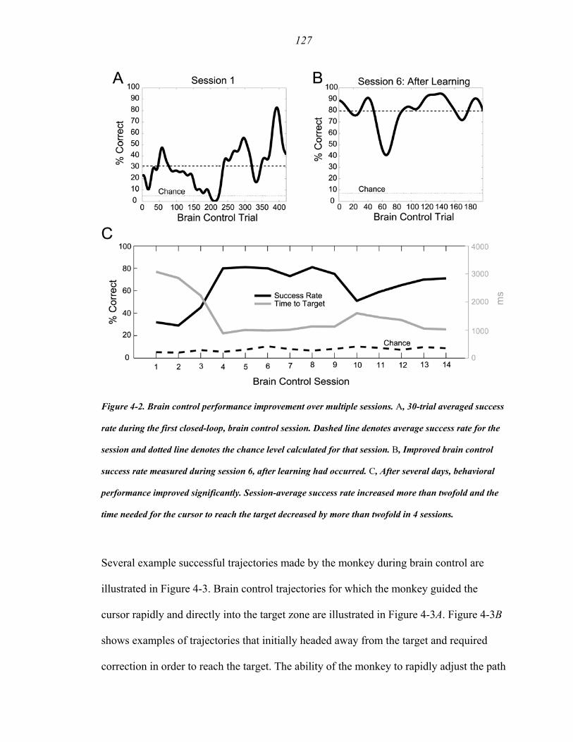
127
Figure 4-2. Brain control performance improvement over multiple sessions. A, 30-trial averaged success
rate during the first closed-loop, brain control session. Dashed line denotes average success rate for the
session and dotted line denotes the chance level calculated for that session. B, Improved brain control
success rate measured during session 6, after learning had occurred. C, After several days, behavioral
performance improved significantly. Session-average success rate increased more than twofold and the
time needed for the cursor to reach the target decreased by more than twofold in 4 sessions.
Several example successful trajectories made by the monkey during brain control are
illustrated in Figure 4-3. Brain control trajectories for which the monkey guided the
cursor rapidly and directly into the target zone are illustrated in Figure 4-3A. Figure 4-3B
shows examples of trajectories that initially headed away from the target and required
correction in order to reach the target. The ability of the monkey to rapidly adjust the path

128
online suggests that he learned to modulate his neural activity in order to steer the cursor
to the goal using continuous feedback of the visual error.

129
Figure 4-3. Examples of successful brain control trajectories during session 8, illustrating trajectories
directed toward the target (A) as well as trajectories that initially headed off-course and therefore
required online correction (B). Brain control targets were made approximately twice as large as target

130
stimuli presented during the training segment (i.e., during joystick trials) in order to allow the monkey to
perform the task successfully during early brain control sessions. So that behavioral performance and
learning effects could be compared fairly across multiple sessions, we kept the target size constant, even
after performance had improved.
4.4.2 Brain control learning effects
Changes in neural activity were monitored in parallel with behavioral performance trends
by analyzing PPC population activity recorded during each session’s joystick training
segment, prior to the brain control segment. Specifically, we averaged the learning effects
across all neural units that were included in a session’s ensemble. Importantly, when
defining the PPC ensemble used for offline decoding assessment, we did not assume that
we recorded from exactly the same ensemble of neural units from session to session
(though this probably occurred to some extent) because: 1) we did not continuously track
the spike waveforms 24 hours per day so as to ensure that neurons were identical and 2) it
is difficult to robustly determine to what extent multi-unit activity consistently reflected
the same combination of single-units from day to day. Instead, for each session we chose
to include only those neural units whose spike waveform signal-to-noise ratio (SNR)
exceeded some arbitrary threshold value (see Methods) when decoding offline. In
general, the average SNR value for an ensemble (2.7 ± 0.08) as well as the number of
single-units (5.9 ± 2.9) did not vary significantly over the course of 14 brain control
sessions, nor did we any observe any significant linear trend in their respective values
(The slopes of line fits for these two trends were not significantly different from zero, that
is the 95 % confidence intervals (CI) of the slope included zero).

131
We observed noteworthy changes in the neural activity that demonstrated strong evidence
of learning in the PPC population. First, we calculated the average R2 for decoding cursor
position from the ensemble (offline analysis using ridge filter), which is illustrated for all
14 sessions in Figure 4-4A. Notice that the R2 trend approximately followed the trend for
behavioral performance, increasing shortly after the first brain control session and
leveling off after several more sessions. The maximal session R2 using ridge regression
was 0.64 (or R2 = 0.80 if G-Kalman had been used), more than doubling the decode
performance obtained on the first day of brain control, which had an R2 of 0.25. The
offline decoding R2 was strongly correlated with online brain control performance on a
session-by-session basis (ρ = 0.60, p = 0.02, Pearson correlation coefficient). This result
suggests that when presented with continuous visual feedback about the decoded position
of the cursor during brain control, PPC neurons were able to collectively modify/improve
their encoding properties (as evidenced by an increase in offline decoding performance),
effectively making more information available to the ridge filter for controlling the cursor
during subsequent brain control sessions.
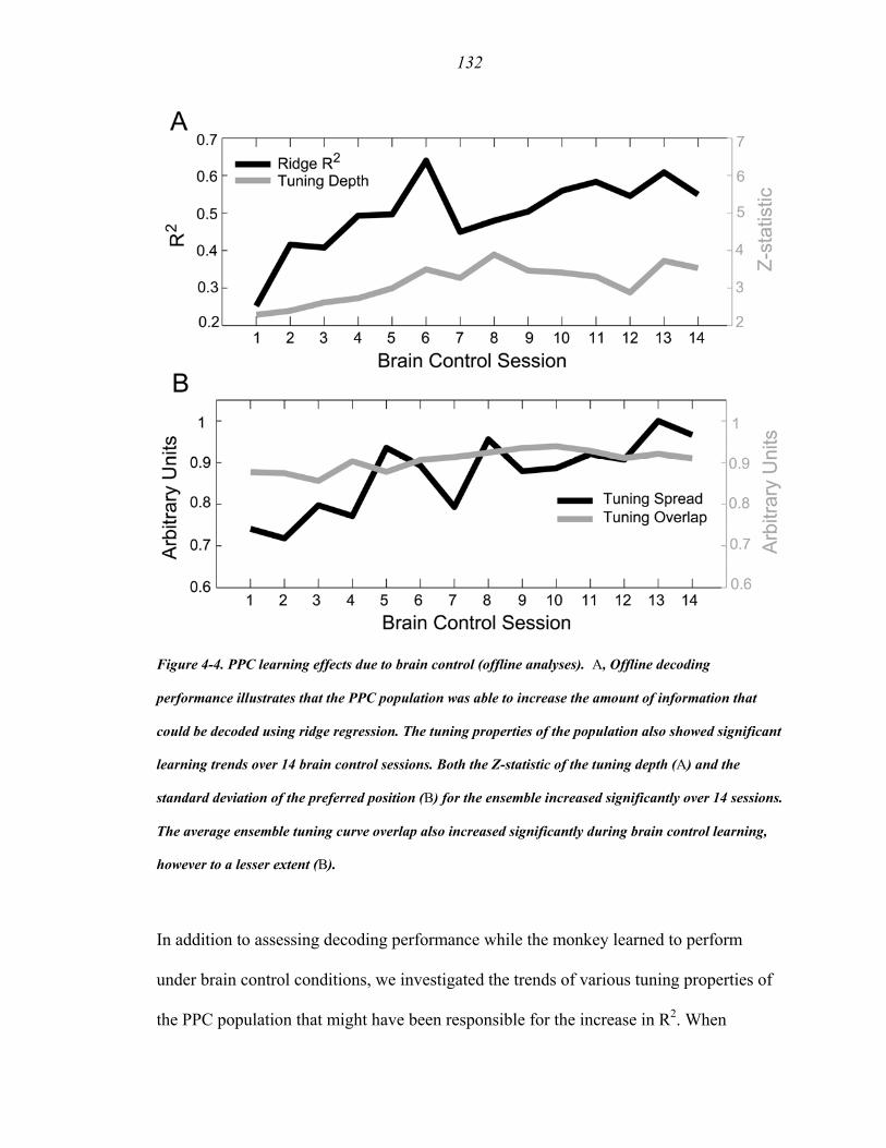
132
Figure 4-4. PPC learning effects due to brain control (offline analyses). A, Offline decoding
performance illustrates that the PPC population was able to increase the amount of information that
could be decoded using ridge regression. The tuning properties of the population also showed significant
learning trends over 14 brain control sessions. Both the Z-statistic of the tuning depth (A) and the
standard deviation of the preferred position (B) for the ensemble increased significantly over 14 sessions.
The average ensemble tuning curve overlap also increased significantly during brain control learning,
however to a lesser extent (B).
In addition to assessing decoding performance while the monkey learned to perform
under brain control conditions, we investigated the trends of various tuning properties of
the PPC population that might have been responsible for the increase in R2. When

133
assessing changes in tuning, we included only the most informative neural units in the
ensemble as determined by the effective degrees of freedom provided by the ridge model
(i.e., the subset of the original ensemble that contributed most significantly during offline
and online decoding, Ndf = 77 ± 20 neural units, mean ± sd). For each joystick training
session, we constructed a 2D position tuning curve for each neural unit in the ensemble;
using firing rates belonging only to the most recent lag time bin. (Note that similar results
were obtained for all three lag time bins, but strongest tuning was typically observed for
the first lag time bin). X and Y cursor positions were discretized into a 6 x 6 array of 36
bins, extending ±10 deg in the X-Y plane. Accordingly, each X-Y bin contained a
distribution of firing rate samples corresponding to sample cursor positions measured at a
particular 2D position (typically > 50 samples). First, to quantify the tuning depth, we
performed a non-parametric Wilcoxon rank sum test (normal approximation method)
using the two firing rate bin distributions that contained the maximum and minimum
mean values. The normal Z-statistic that resulted from this test was defined as the tuning
depth of the position tuning curve. Using this metric, we then computed the ensemble’s
average tuning depth for each session. We found that tuning depth increased most
substantially over the first 8 brain control sessions (by approximately 70%) and
approximately leveled off for the remaining sessions. When fitting a line to this
increasing trend, we found that the slope was significantly larger than zero (m = 0.09,
95% CI : 0.04, 0.14). An increase in ensemble tuning depth can be interpreted as an
expansion of the firing rate dynamic range, boosting the effective gain of the ensemble
for the purpose of encoding position (Fig. 4-4A). Second, we quantified the spread of 2D
tuning for the PPC population by calculating the sd of the preferred positions of all neural
134
units in an ensemble. The preferred position of a neural unit was defined as the X and Y
position that corresponded to the bin with the maximum average firing rate. To obtain a
scalar measure for dispersion, we averaged the sd of the X and Y preferred position
distributions. Similar to the trend we observed for tuning depth, we found that the
average spread of preferred positions increased significantly throughout the brain control
sessions (Fig. 4-4B), ultimately to about 35% above its starting level). The slope of a line
fit to this trend was also significantly larger than zero (m = 2.11, 95% CI : 1.18, 3.04).
This increase in the spread of tuning by the PPC population presumably enabled the
monkey to control the cursor over an increasingly broader range of 2D space on the
computer screen during brain control. Third, we tracked the tuning curve overlap between
all possible pairs of neural units in an ensemble, which were then averaged to give a
scalar ensemble tuning overlap value. We found that the ensemble tuning overlap
increased only slightly (by approximately 6%, Fig. 4-4B), but significantly, over 14 brain
control sessions (m = 0.004, 95% CI : 0.002, 0.007). This increase in ensemble tuning
overlap suggests that the PPC population code became slightly more redundant during
brain control learning.
Summarizing these trends in position tuning, we found that both the tuning depth and
tuning spread of the ensemble increased substantially during brain control. Importantly,
both tuning depth and tuning spread showed strong correlations with R2 decoding
performance, which were highly significant (ρ = 0.71, p = 0.004 and ρ = 0.73, p = 0.003,
respectively, Pearson’s linear correlation coefficient), and consequently with brain
control performance as well (ρ = 0.68, p = 0.007 and ρ = 0.61, p = 0.02, respectively).

135
These correlation results suggest that adjustment of these particular tuning properties was
necessary in order for the ensemble to improve offline decoding performance, and
ultimately for the monkey to improve his performance during brain control. Tuning
overlap was also correlated with R2 performance (ρ = 0.62, p = 0.02). (Note however that
tuning overlap showed a weaker (and less significant) correlation with brain control
performance (ρ = 0.46, p = 0.09)). An increase in tuning depth probably reflected the fact
that more neural units became significantly tuned over the course of the 14 brain
sessions, thereby increasing the likelihood of overlapping tuning curves within the
ensemble. However, it is also possible that the population deliberately broadened the
average width of a typical neural unit’s tuning curve. Unfortunately, this possibility was
difficult to evaluate with our data as positional tuning curves generally comprised a
variety of functional forms, including planar, single-peaked, and occasionally multi-
peaked representations. Future studies will need to address the extent to which
redundancy in the population arises due to an increase in the percentage of tuned neural
units in the ensemble vs. a broadening of the tuning curves of those constituent neural
units.
Finally, it is unlikely that the improvement in R2 performance and enhanced ensemble
tuning was trivially due to a sudden increase in newly appearing neurons that happened to
have stronger tuning properties than previously recorded ensembles. First, during joystick
sessions prior to the initial brain control session, the offline R2 performance achieved
using the ridge filter fluctuated up and down from day to day, but typically fell within a
limited range. For example, the distribution of performances for the 7 sessions prior to

136
beginning brain control was R2 = 0.27 ± 0.03 (mean ± sd). Secondly, as mentioned
above, the number of single-units and the session SNR did not change significantly
during brain control. Finally, we did not observe a significant correlation between R2 and
the session-averaged SNR (ρ = 0.28, p = 0.33). Therefore, the most reasonable
interpretation of the substantial improvement in decoding performance we observed is
that the information content of the PPC ensemble increased due to plasticity effects
characterized by the changes in tuning we reported, and did not occur by the sudden
chance appearance of new, tuned neurons at the tips of our electrodes.
4.5 Discussion
In this study, we showed for the first time that PPC can be used independently to control
a cursor in real-time for a neural prosthetic application. Furthermore, we observed
significant and rapid learning effects in PPC during brain control, which enabled the
monkey to substantially improve behavioral performance over several sessions.
4.5.1 Learning to control a cursor using continuous visual feedback
Operant conditioning of neurons in the primary motor cortex was originally pioneered in
the 1970s, whereby investigators were able to condition the tuning of individual neurons
by directly manipulating the reward the animals received for different responses. (E. E.
Fetz, 1969; E. M. Schmidt et al., 1978). More recently, M1 population learning effects
have been reported while monkeys learned to perform closed-loop brain control
trajectories (D. M. Taylor et al., 2002; J. M. Carmena et al., 2003; M. A. Lebedev et al.,

137
2005). To date however, there has been little if any emphasis placed on learning effects
that occur in PPC during neural prosthetic applications.
Learning effects in PPC became evident quite early during brain control sessions, more
than doubling the offline decoding performance (R2) of the population after 5-6 sessions.
Studies in M1 have reported brain control learning effects of comparable magnitude to
the R2 changes we observed here, however, these changes typically occurred over the
course of 20 sessions or more (D. M. Taylor et al., 2002; J. M. Carmena et al., 2003). In
particular, Carmena and colleagues reported significant learning effects in multiple
cortical areas, including PMd, primary somatosensory cortex (S1) and supplementary
motor area (SMA) during brain control. However, they did not report any change in R2
decoding performance for parietal cortex. Instead, they reported relatively small changes
(approximately 25-30 % increase over 14 sessions) in the tuning depth of parietal neurons
as compared to motor cortex cells which approximately doubled (100% increase) their
tuning depth over the same time period. Therefore, limited conclusions can be drawn
about PPC learning from their data, which suggest that only minor learning effects
occurred in PPC during brain control. In contrast, our data suggest that substantial
learning can occur in PPC over the course of just several brain control sessions (e.g., R2
more than doubled and tuning depth increased by roughly 70%). The discrepancy in
learning evidence between these two studies may reflect the poor quality of the PPC
sample used in the Carmena study relative to samples obtained from other brain areas
from which they recorded. As a result, brain control estimates of cursor position in their
study may have relied more heavily upon contributions from areas other than PPC (e.g.,
138
M1), and thus learning was consequently driven more strongly in those areas. Secondly,
Carmena and colleagues did not control for eye position in their study. Therefore, it is
unclear how eye position or a plan to make a saccade might have influenced neural
activity in PPC. Finally, the extent to which plasticity occurs in different brain areas
during brain control conditions remains an important direction for future experiments.
We expect, based on our findings here and PPC’s known functional role in combining
visual and motor representations, that PPC will be particularly well-suited to serve as a
target for a prosthesis that relies upon visually-guided feedback for continuous control
and error-driven learning.
References
Batista AP, Buneo CA, Snyder LH, Andersen RA (1999) Reach plans in eye-centered coordinates. Science 285:257-260.
Carmena JM, Lebedev MA, Crist RE, O'Doherty JE, Santucci DM, Dimitrov DF, Patil PG, Henriquez CS, Nicolelis MAL (2003) Learning to control a brain-machine interface for reaching and grasping by primates. PLOS Biology 1:193-208.
Fetz EE (1969) Operant Conditioning of Cortical Unit Activity. Science 163:955-958. Hochberg LR, Serruya MD, Friehs GM, Mukand JA, Saleh M, Caplan AH, Branner A,
Chen D, Penn RD, Donoghue JP (2006) Neuronal ensemble control of prosthetic devices by a human with tetraplegia. Nature 442:164-171.
Kennedy PR, Bakay RAE, Moore MM, Adams K, Goldwaithe J (2000) Direct control of a computer from the human central nervous system. IEEE Transactions on Rehabilitation Engineering 8:198-202.
Lebedev MA, Carmena JM, O'Doherty JE, Zacksenhouse M, Henriquez CS, Principe JC, Nicolelis MAL (2005) Cortical ensemble adaptation to represent velocity of an artificial actuator controlled by a brain-machine interface. Journal of Neuroscience 25:4681-4693.
Musallam S, Corneil BD, Greger B, Scherberger H, Andersen RA (2004) Cognitive control signals for neural prosthetics. Science 305:258-262.
Patil PG, Carmena LM, Nicolelis MAL, Turner DA (2004) Ensemble recordings of human subcortical neurons as a source of motor control signals for a brain-machine interface. Neurosurgery 55:27-35.
Santhanam G, Ryu SI, Yu BM, Afshar A, Shenoy KV (2006) A high-performance brain-computer interface. Nature 442:195-198.

139
Schmidt EM, Mcintosh JS, Durelli L, Bak MJ (1978) Fine Control of Operantly Conditioned Firing Patterns of Cortical-Neurons. Experimental Neurology 61:349-369.
Serruya MD, Hatsopoulos NG, Paninski L, Fellows MR, Donoghue JP (2002) Instant neural control of a movement signal. Nature 416:141-142.
Shenoy KV, Meeker D, Cao SY, Kureshi SA, Pesaran B, Buneo CA, Batista AR, Mitra PP, Burdick JW, Andersen RA (2003) Neural prosthetic control signals from plan activity. Neuroreport 14:591-596.
Taylor DM, Tillery SIH, Schwartz AB (2002) Direct cortical control of 3D neuroprosthetic devices. Science 296:1829-1832.
Wessberg J, Stambaugh CR, Kralik JD, Beck PD, Laubach M, Chapin JK, Kim J, Biggs J, Srinivasan MA, Nicolelis MAL (2000) Real-time prediction of hand trajectory by ensembles of cortical neurons in primates. Nature 408:361-365.
Wolpaw JR, McFarland DJ (2004) Control of a two-dimensional movement signal by a noninvasive brain-computer interface in humans. Proceedings of the National Academy of Sciences of the United States of America 101:17849-17854.

140
Chapter 5
CONCLUDING REMARKS
The preceding chapters describe the key contributions from my thesis research. In the
following remarks, I will summarize the significant contributions of my findings and
highlight interesting questions to be addressed in future studies.
5.1 Encoding properties of PPC neurons during online control of movement
5.1.1 Summary of significant findings
PPC is a critical node for the online control of movement. The information theoretic
analysis of Chapter 2 indicates that the population of neurons in PPC is largely
responsible for monitoring the current state of the movement during goal-directed arm
movements. This internal representation of the instantaneous state of the effector is not
compatible with a passive sensory representation of feedback originating from muscle
spindles or the retinae, nor is it probable that these signals represent feedforward motor
commands that causally drive the next state of movement. Instead, such a dynamic
encoding scheme is in agreement with PPC serving as an internal forward model, which
derives the expected state of the effector from knowledge of recently issued motor
commands and the previous state of the effector. These data represent the first
neurophysiological evidence that a forward model of the arm exists in the brain.
Secondly, the application of information theory to the study of temporal encoding

141
properties of motor parameters in non-human primates is relatively new, and has
previously been applied only in M1 (L. Paninski et al., 2004).
The spatiotemporal analysis of Chapter 2 demonstrates that the tuning properties of PPC
neurons reflect rather simple computational primitives. That is, for our task the
movement angle STTFs do not reflect complex paths in space but instead encode
straight-line trajectories. We used a variety of quantitative tools to assess the structure of
these movement angle STTFs, including preferred direction and curvature metrics, as
well as SVD analyses to assess separability. These methods have not been applied
previously for assessing space-time tuning properties of PPC neurons during goal-
directed arm movements. In the future these basis function-like representations may
prove useful for theoretical studies aimed at building network-level models of PPC
computation during online sensorimotor control.
5.1.2 Directions for further investigation
While the temporal encoding properties of movement angle neurons in PPC are
compatible with the output of a theoretical forward model, it is difficult to discern to what
extent the forward model output is related to the state of the cursor on the computer
screen or the physical state of the hand. One possible way to test for a visual vs. motor-
based reference frame would be to dissociate the movement of the cursor from that of the
hand, so that they are incongruent. Information theoretic analyses could again be used to
determine which reference frame is more strongly encoded by PPC neurons.

142
It would be nice to uncover some additional evidence of the efference copy signal being
input to PPC. Simultaneously monitoring the spiking activity and local field potential
(LFP) in other motor areas while recording from PPC, especially the dorsal premotor
cortex (PMd) and primary motor cortex (M1), may provide some additional correlational
evidence for efference copy projections to PPC. For example, the spike-field coherence
between M1 and PPC (specifically phase information) may provide additional insight
into the directionality of information flow between frontal and parietal areas during
online state estimation. However, causal evidence of the existence of efference copy to
PPC would be more compelling. For instance, inactivation of M1 and/or PMd may be
revealing in that any efference copy sent to PPC would likely be blocked in such a
situation. As a result, a forward model in PPC would be forced to operate without access
to efference copy and therefore be critically limited in its ability to make rapid,
anticipatory state estimates. One would expect that in this situation, the accuracy of the
state estimate and therefore the amount of information encoded by PPC movement angle
neurons would decrease. Secondly, it is also possible that the optimal lag times of
movement angle neurons in PPC would shift to become more negative, reflecting a
heavier reliance upon sensory information when previous motor commands are no longer
available.
Finally, an obvious extension of this work is to test the existence of a forward model
estimate in 3D space. One would expect that since reach commands are generally
specified as paths in 3D space that a forward model should also operate in 3D.

143
5.2 Trajectory decoding and a PPC neural prosthetic
5.2.1 Summary of significant findings
PPC ensembles were used to successfully predict the trajectory of an arm movement. We
found that with only 5 neurons we could account for more than 70% of the variance in
cursor position when reconstructing center-out trajectories using a goal-based Kalman
filter. The effectiveness of the goal-based Kalman filter demonstrated that target
information, which is also present in PPC during an arm movement, can be harnessed to
further improve the accuracy of a state estimate. We also demonstrated, for the first time
that PPC can be used independently to drive the desired movement of a cursor on a
computer screen using only the monkey’s thoughts. The monkey learned to control the
neural prosthetic very well, guiding the cursor to 8 randomly selected targets with 80%
success rate. Accompanying this improvement in behavioral performance, we observed
plasticity effects in the PPC ensemble as well, whereby the offline decoding performance,
the overall tuning depth and the 2D coverage of the PPC ensemble increased significantly
over several sessions. These results represent the first proof-of-concept for a neural
prosthetic targeting PPC for continuous neural control of a cursor.
5.2.2 Directions for further investigation
There are several important scientific extensions to my decoding work that will facilitate
further development and smoother transfer of this technology to the clinic. First, the 2D
experiment reported here needs to be performed in a 3D environment. 3D experiments
have been successfully performed before using activity recorded in M1 (D. M. Taylor et

144
al., 2002). Second, an attempt to simulate more natural conditions should be made. There
are several factors that should be considered to address this issue.
1) The eyes should be freed, so that the monkey can look to the target, and then back to
the hand etc. This will undoubtedly bring up interesting challenges when interpreting the
coordinate frame encoding scheme used by PPC during sensorimotor control. For
example, it must first be verified whether eye-centered representations of the state of the
arm/cursor and the target are updated during a saccade. Batista and colleagues showed
evidence for the updating of visual space when monkeys made an intervening saccade
prior to an ensuing reach. However, updating has not been investigated during continuous
control of an end effector (A. P. Batista et al., 1999). Additionally, it has been shown that
a change in eye position can result in gain modulatory effects of neural responses in PPC,
which are likely to be important for coordinate transformations that take place in PPC (R.
A. Andersen et al., 1985). For example, gain modulation is likely important for
transforming eye-centered representations into a representation in hand, or body-centered
coordinates (J. Xing and R. A. Andersen, 2000). Since cells in area 5 have been shown to
encode intended reaches in a combination of eye and hand-centered representations, it is
likely that gain modulation effects will be observed in those neurons as well during a free
gaze task. It will be interesting to test the extent to which visual updating and gain
modulation effects occur in PPC during online control of movement with free gaze.
2) For the reaction tasks studied in this thesis the initiation of an arm movement was
determined by the onset of a target stimulus. It would be interesting modify the task so
145
that it was self-paced, such that the monkey could guide the cursor to a target whenever
he desired to do so. Under these circumstances, the decoder would need to detect the
cognitive event transitions that indicate when a monkey was ‘resting’, planning a
movement, or initiating a movement. Hudson and Burdick have begun work in this
direction and have successfully decoded the event transitions that occur during a standard
memory period reach task (i.e., cue onset, delay, movement period, etc.). In the future, it
will be important to apply these methods to more natural, self-paced tasks appropriate for
a clinical application.
3) Finally, the ability to control the continuous motion of a variety of end effectors,
which have a diverse range of dynamics, should be tested using PPC signals. In principle,
PPC’s more cognitive, visuomotor representation of movement should be suitable for
controlling a variety of objects in the world beyond computer cursors, as demonstrated in
this thesis.
References
Andersen RA, Essick GK, Siegel RM (1985) Encoding of Spatial Location by Posterior Parietal Neurons. Science 230:456-458.
Batista AP, Buneo CA, Snyder LH, Andersen RA (1999) Reach plans in eye-centered coordinates. Science 285:257-260.
Paninski L, Fellows MR, Hatsopoulos NG, Donoghue JP (2004) Spatiotemporal tuning of motor cortical neurons for hand position and velocity. J Neurophysiol 91:515-532.
Taylor DM, Tillery SIH, Schwartz AB (2002) Direct cortical control of 3D neuroprosthetic devices. Science 296:1829-1832.
Xing J, Andersen RA (2000) Models of the posterior parietal cortex which perform multimodal integration and represent space in several coordinate frames. Journal of Cognitive Neuroscience 12:601-614.