continuous friction measurement equipment as a tool … · continuous friction measurement...

VIRGINIA CENTER FOR TRANSPORTATION INNOVATION AND RESEARCH

530 Edgemont Road, Charlottesville, VA 22903-2454

www. VTRC.net

Continuous Friction Measurement Equipment As a Tool for Improving Crash Rate Prediction: A Pilot Study

http://www.virginiadot.org/vtrc/main/online_reports/pdf/16-r8.pdf EDGAR DE LEÓN IZEPPI, Ph.D. Senior Research Associate Center for Sustainable Transportation Infrastructure Virginia Tech Transportation Institute SAMER W. KATICHA, Ph.D. Senior Research Associate Center for Sustainable Transportation Infrastructure Virginia Tech Transportation Institute GERARDO W. FLINTSCH, Ph.D., P.E. Professor of Civil and Environmental Engineering Director of the Center for Sustainable Transportation Infrastructure Virginia Tech Transportation Institute ROSS MCCARTHY Graduate Research Assistant Center for Sustainable Transportation Infrastructure Virginia Tech Transportation Institute KEVIN K. MCGHEE, P.E. Associate Principal Research Scientist Virginia Transportation Research Council Final Report VTRC 16-R8

Standard Title Page – Report on State Project

Report No.: VTRC 16-R8

Report Date: January 2016

No. of Pages: 40

Type of Report: Final Contract

Project No.: RC00069

Period Covered: 08/15/2013 – 04/30/15

Contract No.:

Title: Continuous Friction Measurement Equipment As a Tool for Improving Crash Rate Prediction: A Pilot Study

Key Words: pavement, friction, safety, crashes and crash rates

Author(s): Edgar de León Izeppi, Ph.D., Samer W. Katicha, Ph.D., Gerardo W. Flintsch, Ph.D., P.E., Ross McCarthy, and Kevin K. McGhee, P.E.

Performing Organization Name and Address: Virginia Tech Transportation Institute 3500 Transportation Research Plaza (0536) Blacksburg, VA 24061

Sponsoring Agencies’ Name and Address: Virginia Department of Transportation 1401 E. Broad Street Richmond, VA 23219

Supplementary Notes:

Abstract: A comprehensive pavement management system includes a Pavement Friction Management Program (PFMP) to ensure pavement surfaces are designed, constructed, and maintained to minimize friction-related crashes in a cost-effective manner. The Federal Highway Administration’s (FHWA) Technical Advisory 5040.38 on Pavement Friction Management supersedes a previous advisory that focused on skid crash reduction. In addition to traditional locked-wheel friction-testing devices, this new advisory recommends continuous friction measuring equipment (CFME) as an appropriate method for evaluating pavements. The study described in this report developed a pavement friction inventory for a single construction district in Virginia using the Grip Tester, a low-cost CFME. The continuous friction data were then coupled with crash records to develop a strategy for network analysis that could use friction to improve the ability to predict crash rates. The crash rate analysis applied the well-established methodology suggested by the FHWA for the identification of high crash risk areas using safety performance functions (SPFs), which include empirical Bayes rate estimation from observed crashes. The current Virginia Department of Transportation SPF models were modified to include skid resistance and radius of curvature (interstate and primary system only) to improve the predictive power of the models. A variation of the same methodology was also used to contrast the effect of two different friction repair treatments, i.e., conventional asphalt overlay and high friction surface treatments, to explore how their strategic use can impact network level crash rates. The result suggests significant crash reductions with comprehensive economic savings of $100 million or more when applied to a single relatively rural district. These findings easily justify an aggressive state-level PFMP and further support continued research to quantify the influence of other pavement-related characteristics such as macrotexture, grade, and cross-slope.

FINAL REPORT

CONTINUOUS FRICTION MEASUREMENT EQUIPMENT AS A TOOL

FOR IMPROVING CRASH RATE PREDICTION: A PILOT STUDY

Edgar de León Izeppi, Ph.D.

Senior Research Associate

Center for Sustainable Transportation Infrastructure

Virginia Tech Transportation Institute

Samer W. Katicha, Ph.D.




Gerardo W. Flintsch, Ph.D., P.E.

Professor of Civil and Environmental Engineering

Director of the Center for Sustainable Transportation Infrastructure


Ross McCarthy

Graduate Research Assistant



Kevin K. McGhee, P.E.

Associate Principal Research Scientist

Virginia Transportation Research Council

Project Manager

Michael M. Sprinkel, P.E., Virginia Transportation Research Council


(A partnership of the Virginia Department of Transportation and

the University of Virginia since 1948)

Charlottesville, Virginia

January 2016

VTRC 16-R8

ii

DISCLAIMER

The project that is the subject of this report was done under contract for the Virginia

Department of Transportation, Virginia Transportation Research Council. The contents of this

report reflect the views of the authors, who are responsible for the facts and the accuracy of the

data presented herein. The contents do not necessarily reflect the official views or policies of the

Virginia Department of Transportation, the Commonwealth Transportation Board, or the Federal

Highway Administration. This report does not constitute a standard, specification, or regulation.

Any inclusion of manufacturer names, trade names, or trademarks is for identification purposes

only and is not to be considered an endorsement.

Each contract report is peer reviewed and accepted for publication by staff of Virginia

Transportation Research Council with expertise in related technical areas. Final editing and

proofreading of the report are performed by the contractor.

Copyright 2016 by the Commonwealth of Virginia.

All rights reserved.

iii

ABSTRACT

A comprehensive pavement management system includes a Pavement Friction

Management Program (PFMP) to ensure pavement surfaces are designed, constructed, and

maintained to minimize friction-related crashes in a cost-effective manner. The Federal

Highway Administration’s (FHWA) Technical Advisory 5040.38 on Pavement Friction

Management supersedes a previous advisory that focused on skid crash reduction. In addition to

traditional locked-wheel friction-testing devices, this new advisory recommends continuous

friction measuring equipment (CFME) as an appropriate method for evaluating pavements.

The study described in this report developed a pavement friction inventory for a single

construction district in Virginia using the Grip Tester, a low-cost CFME. The continuous

friction data were then coupled with crash records to develop a strategy for network analysis that

could use friction to improve the ability to predict crash rates.

The crash rate analysis applied the well-established methodology suggested by the

FHWA for the identification of high crash risk areas using safety performance functions (SPFs),

which include empirical Bayes rate estimation from observed crashes. The current Virginia

Department of Transportation SPF models were modified to include skid resistance and radius of

curvature (interstate and primary system only) to improve the predictive power of the models. A

variation of the same methodology was also used to contrast the effect of two different friction

repair treatments, i.e., conventional asphalt overlay and high friction surface treatments, to

explore how their strategic use can impact network level crash rates. The result suggests

significant crash reductions with comprehensive economic savings of $100 million or more when

applied to a single relatively rural district.

These findings easily justify an aggressive state-level PFMP and further support

continued research to quantify the influence of other pavement-related characteristics such as

macrotexture, grade, and cross-slope.

1

FINAL REPORT

CONTINUOUS FRICTION MEASUREMENT EQUIPMENT AS A TOOL

FOR IMPROVING CRASH RATE PREDICTION: A PILOT STUDY

Edgar de León Izeppi, Ph.D.




Samer W. Katicha, Ph.D.




Gerardo W. Flintsch, Ph.D., P.E.

Professor of Civil and Environmental Engineering

Director of the Center for Sustainable Transportation Infrastructure


Ross McCarthy

Graduate Research Assistant



Kevin K. McGhee, P.E.

Associate Principal Research Scientist


INTRODUCTION

Background

In 1980, the Federal Highway Administration (FHWA) issued Technical Advisory

5040.17: Skid Accident Reduction Program as a general overview of factors that should be

considered as part of the Highway Safety Program Standard 12 (HSPS-12) that required every

state to have a program of highway design, construction, and maintenance to improve highway

safety. HSPS-12 provided pavement friction directives and also emphasized the need for

resurfacing or other surface treatment with emphasis on correction of locations or sections of

streets and highways with low skid resistance and high or potentially high accident rates

susceptible to reduction by providing improved surfaces. In particular, it stated that the purpose

of a skid accident reduction program focused mainly on minimizing the wet weather skidding

accidents. In Virginia, as in many other states, this program functioned under the name Wet

Accident Reduction Program (WARP).

2

In 2005, The Safe, Accountable, Flexible, and Efficient Transportation Equity Act: A

Legacy for Users (SAFETEA-LU) established the Highway Safety Improvement Program

(HSIP) “to achieve a significant reduction in traffic fatalities and serious injuries on public

roads” (FHWA, 2013a). To use the HSIP funds, states were required to develop Strategic

Highway Safety Plans (SHSPs), establish a crash data system, and annually report locations with

severe safety needs. In Virginia, the Surface Transportation Safety Executive Committee was

formed in 2006 to integrate and coordinate all transportation safety programs, particularly those

established to comply with the mandates outlined in SAFETEA-LU and the National Highway

Safety Act of 1966. This committee created, implemented, and evaluated the 2006-2010

Commonwealth SHSP (Virginia Department of Transportation [VDOT], 2013).

The Moving Ahead for Progress in the 21st Century Act (MAP-21) continued the goals

of the HSIP, nearly doubling the funds for FY13 and FY14. MAP-21 required a data-driven,

strategic approach to improving highway safety on all public roads that focuses on performance

(FHWA, 2013b). Virginia’s 2012-2016 SHSP and update process has been approved by

FHWA. The new SHSP should be an opportunity to revisit a statement made in the 2006-2010

SHSP regarding Virginia’s transportation safety public policy. In the earlier document, it read:

“Transportation safety public policy in the United States as well as in Virginia has focused on

crash survivability and not crash prevention” (VDOT, 2013).

In 1997, the American Association of State Highway and Transportation Officials

(AASHTO) first approved its SHSP by more than the required two-thirds majority vote; the plan

was revised and updated in 2004. Since then, each state and many organizations have

implemented their own SHSPs. However, AASHTO (with the help of many highway safety

stakeholders) found in 2010 that there is no one strategy that united all SHSPs. The U.S.

Department of Transportation (U.S. DOT), specifically through FHWA, and AASHTO have

since initiated an effort to develop a national approach. This new strategy is called Toward Zero

Deaths: A National Strategy on Highway Safety (U.S. DOT, 2013).

This strategy represents a nationwide effort to eliminate highway fatalities as a threat to

public and personal health. The strategy will be developed with input from a range of highway

safety stakeholders. The end result will comprise two key parts: a national safety plan and an

associated outreach program. A process will be developed for implementing the plan. The

holistic, data-driven plan will include key emphasis areas, projection of future needs, promising

countermeasures, and expected improvements.

Pavement Friction Measurements in Virginia

Virginia has had a long history with measuring tire-pavement friction since its

introduction in the United States and more recently under the state’s WARP (Mahone and

Sherwood, 1996). “ASTM Committee E-17 on Vehicle-Pavement Systems (originally the

Committee on Skid Resistance) had its genesis after the First International Skid Prevention

Conference, held in Charlottesville, Virginia in September 1958, through the efforts of the late

Tilton E. Shelburne,” Virginia Department of Highways first Head of Research (Whitehurst,

2011). Through the efforts of the Virginia Transportation Research Council (VTRC), Virginia

3

helped establish national standards for skid resistance and, in 1976, “developed a procedure for

systematically identifying and evaluating wet crash sites or low skid number sites and

established the WARP. The program procedures are outlined in Virginia’s Wet Accident

Reduction Program: A User’s Manual” (McGovern et al., 2011).

VTRC materials and engineering research continued, but with changes in scope.

VDOT’s Materials Division purchased the first ASTM E-274 Locked-wheel skid trailer in 1974,

equipped with ribbed tires (VDOT, 2009). Since 1988 the Materials Division has grown the skid

testing program in Virginia to include the following areas (Habib, 2012):

Programmatic Testing

Inventory

WARP

Needs-based Testing

Project specific

As needed.

The inventory program is set up to test all interstate and primary routes on a multiyear

cycle, doing two to three districts/year, with a measurement every 0.2 mile. However, data from

inventory testing were last uploaded in 2010 into VDOT’s Highway Traffic Records Inventory

System (HTRIS), a system that was abandoned around 2012. Any new data that might have

been recorded were not transferred into the new Roadway Network System (RNS) program.

Thus, VDOT’s Traffic Engineering Division (TED) has experienced increasing difficulties using

skid testing data to analyze crash locations for much of the last decade. Although testing

resumed in 2014, the last published WARP report that contains any friction testing references

data from 2007 (VDOT, 2009).

As with most state agencies in the United States, Virginia’s program continues to use a

locked-wheel testing device, having switched to a smooth tire (ASTME E-524) in the 1990s.

This device measures friction very well on long pavement sections that are relatively

homogeneous in nature.

The Virginia Strategic Highway Safety Plan (SHSP)

The 2012 update to the Virginia SHSP establishes seven emphasis areas to include:

speeding, young drivers, occupant protection, alcohol-related incidents, roadway departure,

intersections, and data collection, data management, and data analysis (VDOT, 2013).

The SHSP update also reported that from 2001 to 2010, roadway departure and

intersection crashes accounted for 83% of all deaths and 68% of the severe injuries. Strategy 1

under Roadway Departure is to keep vehicles on the road and in their lanes, a goal made far

more achievable with adequate adherence to the traveled surface. Action 1.7 for this strategy

says to “continue to research advances in pavement designs to enhance pavement friction. Seek

opportunities to install high-friction pavements where appropriate, cost effective and practical.”

4

Although the actions for the intersection-related crash strategies do not specifically

mention tire-pavement friction, intersections are where braking, turning, and other extreme

maneuvering is most common and by definition where sufficient tire-pavement friction is most

essential. Finally, Strategy 4 under the Data Emphasis Area Plan specifically addresses

improved tools for highway safety analysis that uses highway inventory and condition data; tire-

pavement friction is among the more fundamental and relevant properties of traveled surfaces.

Pavement Friction Management Programs

In June 2010, FHWA issued the new Technical Advisory 5040.38: Pavement Friction

Management (FHWA, 2010), superseding the previous Technical Advisory 5040.17: Skid

Accident Reduction Program. This new advisory provides guidance to highway agencies

towards developing or improving pavement friction management programs (PFMPs) to ensure

pavement surfaces are designed, constructed, and maintained to provide adequate and durable

friction properties that reduce friction-related crashes in a cost-effective manner. The advisory

lists four types of full-scale friction test equipment:

. . . locked wheel, fixed slip, side force, and variable slip. The locked wheel method (ASTM E-

274) is used widely on US highways and simulates emergency braking without anti-lock brakes.

Many agencies monitor friction on an annual basis or on a 2 or 3 year cycle. The spatial interval

for friction tests is typically 1-2 tests per mile with some US highway agencies performing 3-5

friction tests per mile (FHWA, 2010).

The three remaining methods can be characterized as continuous friction measurement

equipment (CFME) because they collect friction measurements continuously, greatly enhancing

the ability to detect isolated low friction areas on pavements. The side force method evaluates

the ability to maintain control in curves, and similar to the fixed slip and variable slip methods,

relate better to braking with anti-lock brakes. When this advisory was published, side force

friction, fixed and variable slip measurement systems were not readily available or used on U.S.

highways. However, the advantage of these methods over the locked wheel method is the ability

to operate continuously over a test section, especially on curves, and the better relationship to

braking with anti-lock brakes. Because all friction test methods can be insensitive to

macrotexture under specific circumstances, it is recommended that friction testing be

complemented by macrotexture measurement (FHWA, 2010).

In 2010, in support of that directive, the Center for Sustainable Transportation

Infrastructure of the Virginia Tech Transportation Institute (VTTI) initiated the FHWA-funded

research project “Development and Demonstration of Pavement Friction Management

Programs.” The three objectives of this project are (1) to establish investigatory (desirable) and

intervention (minimum) levels for friction and macrotexture for different friction demand

categories or classes of highways; (2) assist at least four states in developing PFMPs; and (3)

demonstrate state-of-the-art friction measurement equipment.

An essential early-project task of the VTTI research was to prepare a written report to

FHWA that recommended the most technically sound type of continuous friction measurement

equipment to manage proactively a network-level pavement friction program (Flintsch et al.,

5

2011). The overriding criterion used was the ability of the recommended equipment to discern

pavement properties that can be addressed to reduce crashes on as much of the network as

possible. The final recommendations called for a sideway force coefficient (SFC) continuous

measuring system with a 2,000-gallon tank able to measure friction between 30 and 60 mph,

with a fixed slip ratio between 30% and 45%, dynamic load measurement capability along both

the vertical and horizontal axes, macrotexture and temperature sensors, and an inertial

differential GPS system capable of providing grade, cross-slope, and radius of curvature at 10-m

intervals. This device is marketed as the SCRIM (Side-Force Coefficient Routine Investigation

Machine) manufactured by W.D.M. Limited in Bristol, England, under license to the UK

Transport Research Laboratory (TRL).

A Recent Review of Virginia’s WARP

In June 2010, when FHWA launched the new PFMP technical advisory, which

emphasizes a network-level approach, the amount of friction testing suggested was significantly

increased. In response to this and other changes in the highway legislation, in October 2012, the

Highway Safety Engineer’s Officer from VDOT’s TED started a review of the WARP and

approached the VTRC Pavement Research Advisory Committee to present their findings on the

limitations to the WARP. As a result of this meeting, VTRC was asked to review the WARP and

“one of WARP’s critical components, the Potential Wet Accident Hotspot (PWAH) procedure,

which identifies locations with elevated wet-weather crash rates relative to comparable

locations” (Cottrell and Kweon, 2013). Among the outcomes from that review were

recommendations to include multiple years of crash data, and to develop safety performance

functions (SPFs) that incorporate predictors such as wet-weather and traffic exposure. Although

not mentioned specifically, friction is another likely predictor of safety performance for

pavements.

PURPOSE AND SCOPE

The purpose of this research was to explore the use of CFME as a principal tool for

pavement friction management. This was accomplished through a district-level pilot that

included collection of an inventory of CFME-based data, reduction of that data to link with other

pavement- and crash-related records, analysis to relate friction (and other) data to crash rates, and

an exercise to demonstrate the economic ramifications of a proactive PFMP.

The researchers initially agreed to make a complete assessment of the pavement friction

program to include CFME testing and comparisons to the locked-wheel skid tester used by

Virginia. Because the locked-wheel tester was not operational during the data collection phase

of the study, the comparisons were limited to operational characteristics. The analysis of the

friction measurements and their relationship to crash data were accomplished and delivered

through enhanced SPFs.

6

METHODS

Friction Data

Collection

VDOT’s Salem District, which contains Virginia Tech, was selected for the pilot. The

first step was to select the roads within the Salem District to survey. A starting point was the

same roads that the Pavement Maintenance System (PMS) surveys each year as part of their road

condition inventory. Every year PMS collects pavement condition data in one lane in each

direction of travel for all divided roads and one lane in only one direction for undivided roads.

These lanes are called directional lane-miles, and PMS collects data along the directional miles

for the three major systems of highways in Virginia: interstate (100%), primary (100%), and

secondary systems (20%, or equivalent to a 5-year cycle).

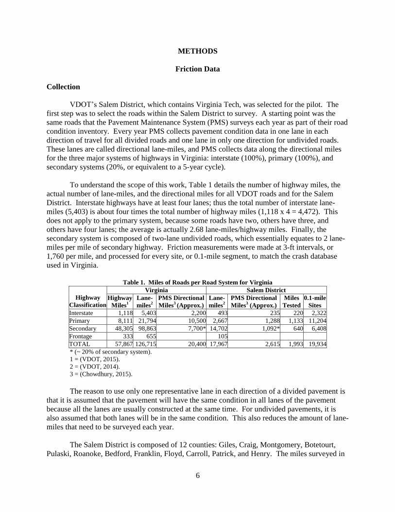
To understand the scope of this work, Table 1 details the number of highway miles, the

actual number of lane-miles, and the directional miles for all VDOT roads and for the Salem

District. Interstate highways have at least four lanes; thus the total number of interstate lane-

miles (5,403) is about four times the total number of highway miles (1,118 x 4 = 4,472). This

does not apply to the primary system, because some roads have two, others have three, and

others have four lanes; the average is actually 2.68 lane-miles/highway miles. Finally, the

secondary system is composed of two-lane undivided roads, which essentially equates to 2 lane-

miles per mile of secondary highway. Friction measurements were made at 3-ft intervals, or

1,760 per mile, and processed for every site, or 0.1-mile segment, to match the crash database

used in Virginia.

Table 1. Miles of Roads per Road System for Virginia

Highway

Classification

Virginia Salem District

Highway

Miles1

Lane-

miles2

PMS Directional

Miles3 (Approx.)

Lane-

miles2

PMS Directional

Miles3 (Approx.)

Miles

Tested

0.1-mile

Sites

Interstate 1,118 5,403 2,200 493 235 220 2,322

Primary 8,111 21,794 10,500 2,667 1,288 1,133 11,204

Secondary 48,305 98,863 7,700* 14,702 1,092* 640 6,408

Frontage 333 655 105

TOTAL 57,867 126,715 20,400 17,967 2,615 1,993 19,934

* (~ 20% of secondary system).

1 = (VDOT, 2015).

2 = (VDOT, 2014).

3 = (Chowdhury, 2015).

The reason to use only one representative lane in each direction of a divided pavement is

that it is assumed that the pavement will have the same condition in all lanes of the pavement

because all the lanes are usually constructed at the same time. For undivided pavements, it is

also assumed that both lanes will be in the same condition. This also reduces the amount of lane-

miles that need to be surveyed each year.

The Salem District is composed of 12 counties: Giles, Craig, Montgomery, Botetourt,

Pulaski, Roanoke, Bedford, Franklin, Floyd, Carroll, Patrick, and Henry. The miles surveyed in

7

the Salem District and the number of lane-miles collected by the PMS surveys is almost equal for

the interstate (IS) and the primary system (PS) but vary significantly in the secondary system.

This is due to the fact that for PMS purposes, the 20% sample is randomly made to reflect

network-level condition. However, this random sampling includes some secondary sites that

have little or no traffic, are dead-end streets, are unpaved, etc. This approach was not considered

appropriate for the study, so a list of the most heavily traveled secondary roads for each county

in the district was obtained from the staff of the Regional Traffic Engineering Department (RTE)

and is provided in Appendix A.

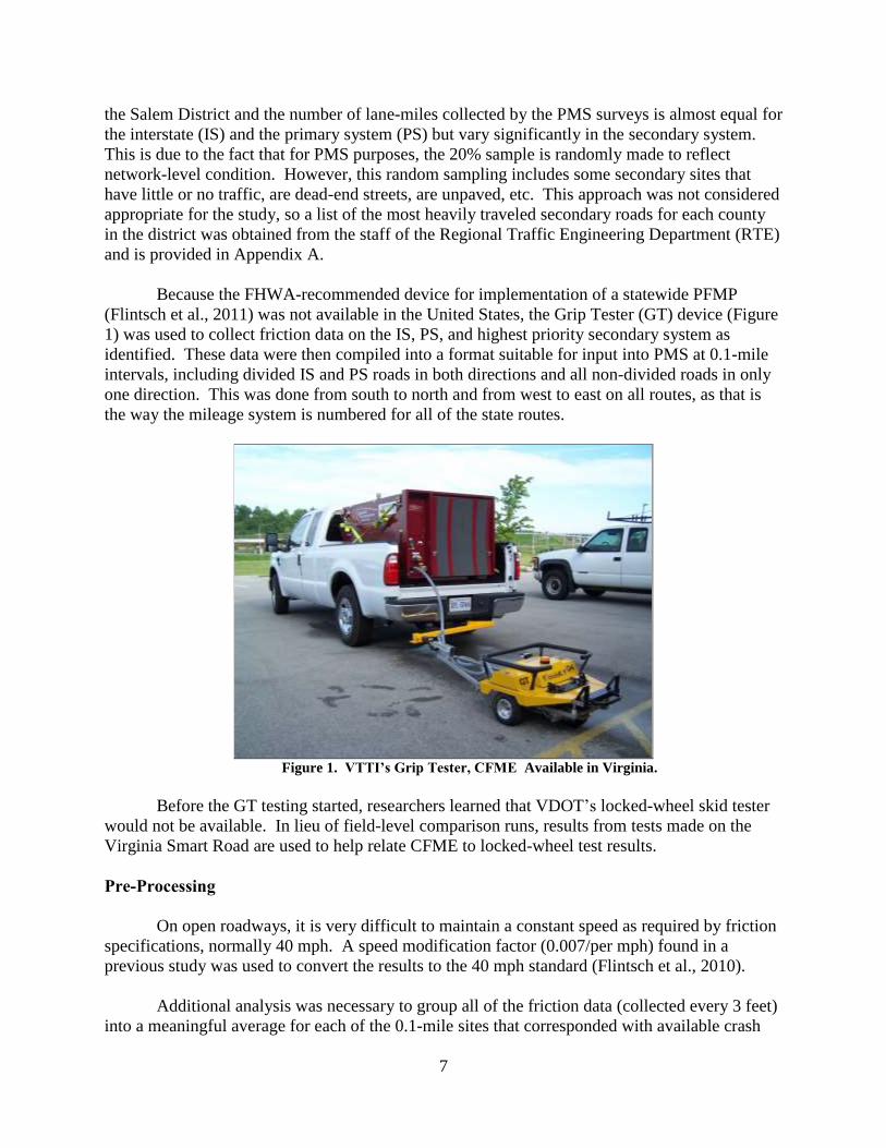
Because the FHWA-recommended device for implementation of a statewide PFMP

(Flintsch et al., 2011) was not available in the United States, the Grip Tester (GT) device (Figure

1) was used to collect friction data on the IS, PS, and highest priority secondary system as

identified. These data were then compiled into a format suitable for input into PMS at 0.1-mile

intervals, including divided IS and PS roads in both directions and all non-divided roads in only

one direction. This was done from south to north and from west to east on all routes, as that is

the way the mileage system is numbered for all of the state routes.

Figure 1. VTTI’s Grip Tester, CFME Available in Virginia.

Before the GT testing started, researchers learned that VDOT’s locked-wheel skid tester

would not be available. In lieu of field-level comparison runs, results from tests made on the

Virginia Smart Road are used to help relate CFME to locked-wheel test results.

Pre-Processing

On open roadways, it is very difficult to maintain a constant speed as required by friction

specifications, normally 40 mph. A speed modification factor (0.007/per mph) found in a

previous study was used to convert the results to the 40 mph standard (Flintsch et al., 2010).

Additional analysis was necessary to group all of the friction data (collected every 3 feet)

into a meaningful average for each of the 0.1-mile sites that corresponded with available crash

8

data. This was accomplished using a moving-average filter of 60 feet for the entire 0.1 mile.

The filter length was selected to align with the locked wheel tester, which reports friction from

an average of 1 second of measurement at 40 mph (59 feet). The analysis then selected the

lowest point in that 0.1-mile moving-average data, which then represents the lowest

measurement that any locked-wheel skid tester could find if it knew exactly where the worst 1-

second average would happen in every 0.1 mile. There are 157 possible 60-feet sections in a 0.1-

mile (528 ft) site, so the chances of a locked-wheel device “finding” that same location are

1/157.

Crash Records

Annual Virginia Data

A breakdown of the 10-year crash data from 2003 to 2012 in Virginia is shown in Table 2

to show that on average every year 82% of crashes occur under dry (clear or cloudy) conditions

compared to only 15% that are considered wet crashes with the remaining (~3%) happening

during snow, ice or hail events. Because the great majority of crashes happen under dry

conditions, it is important that comprehensive crash analysis (to include friction, etc.)

considering all crashes, not just the wet ones. It is also worth noting that on average, the

percentage of fatal crashes, injury, and personal property crashes is 1%, 35%, and 64% of the

total crashes, respectively.

Table 2. Average Crashes in Virginia: 1999-2012 (Commonwealth of Virginia, 2013)

Year 2003 2004 2005 2006 2007 2008 2009 2010 2011 2012 Average

Fatal 860 837 875 865 940 760 694 689 707 714 794

Personal Injury 55,041 55,194 53,727 52,083 49,138 48,887 44,285 43,149 43,993 44,924 49,042

Property Damage 98,947 97,876 99,247 98,744 95,327 85,635 71,765 72,548 75,813 77,941 87,384

Total Crashes 154,848 153,907 153,849 151,692 145,405 135,282 116,744 116,386 120,513 123,579 137,220

Crash Conditions

Dry* 119,444 123,999 126,824 126,756 123,972 110,539 89,433 97,422 100,642 103,702 112,273

Snow 4,703 2,740 4,238 1,445 2,753 1,482 2,656 5,102 1,420 1,612 2,815

Ice (Sleet/Hail) 1,332 771 1,187 56 894 503 758 339 527 386 675

Wet and other** 29,369 26,397 21,600 23,435 17,786 22,758 23,897 13,523 17,924 17,879 21,457

% Dry 77% 81% 82% 84% 85% 82% 77% 84% 84% 84% 82%

% Wet 19% 17% 14% 15% 12% 17% 20% 12% 15% 14% 15%

* Dry (No adverse condition: clear or cloudy and ** Wet and other (rain, fog, mist, etc.).

Salem District

Snow and ice (and sleet/hail) represent conditions in which the tire and pavement are

often at least partially separated by a “contaminant.” Therefore, crashes that happen under these

conditions cannot be attributed to lack of friction on the road, and have been eliminated from the

analysis. When these crashes are not taken into account, the proportion of wet to dry crashes in

the Salem District is 17% to 83%, as can be seen in Table 3. The crash data and average annual

daily traffic (AADT) were obtained from the VDOT Traffic Monitoring System records for each

corresponding 0.1-mile site of pavement where friction was measured. The data for curvature

(radius of curvature on curves sites) were also obtained, only for the interstate and primary

systems, from the PMS database, but it does not include the secondary system.

9

Table 3. Crashes Analyzed in the Salem District (2010-2012)1 by Highway System

Highway

System

Wet and Other* Dry** Analyzed (Wet + Dry)

Total

Crashes

Found

in 0.1-

mile

Sites

Total

0.1-

mile

Sites

Fatalities

Injury

Property

Damage

Fatalities

Injury

Property

Damage

Fatalities

Injury

Property

Damage

Interstate 6 123 324 22 485 1,181 28 608 1,505 2,141 1,189 2,322

Primary 11 242 396 72 1,526 2,597 83 1,768 2,993 4,844 3,072 11,204

Secondary 0 126 209 17 510 783 17 636 992 1,645 1,217 6,408

Total

Crashes

17 491 929 111 2,521 4,561 128 3,012 5,490 8,630 5,478 19,934

Interstate % 0.1% 1.4% 3.8% 0.3% 5.6% 13.7% 0.3% 7.0% 17.4% 24.8%

Primary % 0.1% 2.8% 4.6% 0.8% 17.7% 30.1% 1.0% 20.5% 34.7% 56.1%

Secondary% 0.0% 1.5% 2.4% 0.2% 5.9% 9.1% 0.2% 7.4% 11.5% 19.1%

TOTAL % 0.2% 5.7% 10.8% 1.3% 29.2% 52.9% 1.5% 34.9% 63.6% 100.0%

1 = (Commonwealth of Virginia, 2013).

* Dry (No adverse condition: clear or cloudy and ** Wet and other (rain, fog, mist, etc.).

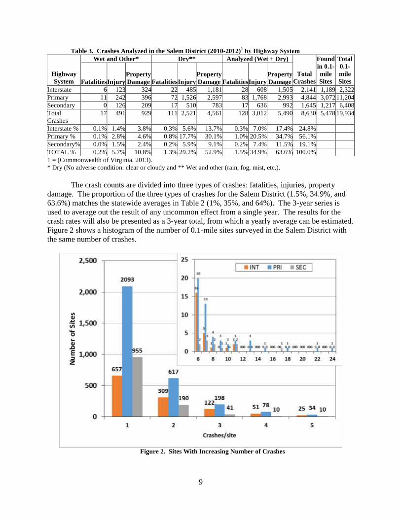
The crash counts are divided into three types of crashes: fatalities, injuries, property

damage. The proportion of the three types of crashes for the Salem District (1.5%, 34.9%, and

63.6%) matches the statewide averages in Table 2 (1%, 35%, and 64%). The 3-year series is

used to average out the result of any uncommon effect from a single year. The results for the

crash rates will also be presented as a 3-year total, from which a yearly average can be estimated.

Figure 2 shows a histogram of the number of 0.1-mile sites surveyed in the Salem District with

the same number of crashes.

Figure 2. Sites With Increasing Number of Crashes

10

The number of sites with high crashes is very low. However, the two sites that have the

maximum number of crashes observed on a site (22 and 24 crashes) are on the primary highway

system.

Modeling of Crash Rates for Individual Pavement Sections

Vehicle crash analysis for network screening is typically analyzed using Poisson or

Poisson-Gamma (Negative Binomial) models, and empirical Bayes (EB) crash rate estimation

from observed crashes and SPFs, as described in the Highway Safety Manual (HSM) predictive

methods (AASHTO, 2008). These terms are mostly unfamiliar to pavement engineers and, in

this section, an intuitive explanation of crash rate modeling and estimation is provided.

Empirical Bayes and Safety Performance Functions

The data obtained from crash records are essentially count data; that is, the data are given

in terms of the number of crashes observed at a specific pavement section (the same 0.1-mile

pavement sections). Crash occurrence is a rare event with an associated very low probability of

occurrence, a probability that will be named p. As such, for every vehicle traversing a 0.1-mile

pavement section (the analysis can be done for other section lengths), there is a (very low)

probability (chance) p that this vehicle will be involved in a crash on that specific section.

Because there are only two possible outcomes, crash or no crash, the observed outcomes

will follow a binomial distribution (e.g., tossing a coin, but with the probability of heads very

small, similar to the chance of winning the lottery). With a very large number of vehicles

traversing the pavement section and a very small p, the binomial distribution converges to the

Poisson distribution. Therefore, the use of the Poisson distribution to model crash rates can be

explained through a logical physical process (that involves chances of occurrence). The Poisson

distribution is parametrized by a rate (average) which represents the rate of crash occurrence.

Parametrized means that it is completely defined by the rate (as a side note, the normal

distribution is parametrized by two parameters, its average and standard deviation).

Highway safety analyses have determined that the crash rate depends on factors such as

traffic, driver behavior, road geometry, pavement characteristics, and others. To find how these

factors affect the rate (Poisson), a regression analysis is performed. In this study, traffic

(expressed as Annual Average Daily Traffic or AADT), pavement friction, and curvature (when

present) were considered as affecting the crash rate. Under the Poisson model assumption, given

the AADT, pavement friction, and pavement curvature, the crash rate at a specific section can be

determined.

In practice, the Poisson model does not fully represent the observed crash count. For the

Poisson model, the variability (variance) of the observations is restricted to be equal to the rate.

Researchers have long observed that the variability (variance) of actual crash data is much larger

than the rate, referring to this phenomenon as over-dispersion (i.e., more variability than what

would be predicted by the Poisson model). The physical explanation for this over-dispersion is

that there are factors other than the ones considered in the regression model that affect the crash

11

rate. In this study, AADT, friction, and curvature were considered and it should be expected that

there are many more factors involved in a crash occurring.

The most common approach that has been used to account for the over-dispersion is to

consider that the crash rate of sites having similar recorded characteristics (AADT, friction, and,

if available, curvature) will vary according to a Gamma distribution (hence the term Poisson-

Gamma, also called Negative Binomial [NB]) which provides significant flexibility in

representing this variation. NB regression can be used to estimate the parameters of the

regression. In general, the parameters will be close to the ones obtained from the Poisson

regression. The advantage of the NB regression is that it also estimates the over-dispersion.

The estimated over-dispersion parameter is what essentially differentiates between the

Poisson model and the NB model. The Poisson model considers that all relevant parameters that

affect the crash rate have been considered in the model. As such the actual crash count on a

pavement section does not provide any additional information about the crash rate as the rate can

be (according to the Poisson model, exactly) calculated from the measured variables (AADT,

friction, and curvature). In the NB model, the calculated rate is not the final estimated rate for a

specific section. It represents the average of similar sections but the actual rate of each of these

sections vary according to the over-dispersion parameter. Therefore, the actual crash count at a

specific section provides additional valuable information about the crash rate at that specific

section. A sensible approach to follow is to somehow combine the information from the model

with the site specific crash count to come up with a better estimate of the true crash rate than

what can be obtained from either the model or crash count alone.

This estimation approach is similar to the engineering method of problem solving that

combines experience with site specific information, commonly known as the Observational

Method (Peck, 1969). The model summarizes the information from all available sites and can be

seen as compiling the engineering experience while the actual crash count is the site specific

information. An experienced engineer knows to combine accumulated knowledge with the site

specific information to come up with a good solution, in contrast with an inexperienced engineer

that only uses site specific information to come up with “erroneous” solutions. If site specific

information is relatively accurate, the experienced engineer will put more weight on this

information and less weight on previous experience. In contrast, if site specific information is

relatively inaccurate, an experienced engineer will place more importance on past experience.

In the modeling approach, the information is combined using Bayes’ theorem. For the

NB model, the Bayes solution turns out to be a simple weighted average of the model prediction

and the actual site specific crash count, the relative weights of each depending on the over-

dispersion. The empirical part of the EB approach refers to the fact that the parameters of the

Gamma distribution, which is the prior, parameters are estimated from the data (using the NB

regression).

For a more in-depth discussion of the models used here, their origins and applications, as

well as more figures related to the different models, thesis work done as part of this research

explains them in more detail than is necessary here (McCarthy, 2015).

12

Regression Analysis With Safety Performance Functions

As explained before, in the United States, the identification of high crash risk areas is

assessed using SPFs, a procedure that is well established by the FHWA and AASHTO. The SPF

used in Equation 1 employs the NB model, requiring the evaluation of AADT as the mandatory

variable, while other factors (i.e., roadway geometry, traffic control features, etc.) are left to the

discretion of the state DOT (Srinivasan and Bauer, 2013).

jio XAADT

eLP 111)ln(

[Eq. 1]

where

P = Expected number of crashes (also referred to as or the crash rate)

AADT = Annual Average Daily Traffic (natural logarithm)

= Independent variables

j = Regression coefficients

L = Road segment length.

In Virginia, the current network screening structure for Equation 1 considers only the

AADT (Kweon and Lim, 2014). Equation 2 shows the variation from Equation 1 as the model

form used for this study. In this model, two additional variables are included in the SPF model,

radius of curvature, CV (interstate and primary routes only) and skid resistance, represented as

GN, or Grip Number. The coefficient o is the intercept term. Since the sectional length is

defined as 0.1 mile (all data adjusted accordingly), the L term is not included here.

3

121)ln(

CVGNAADToe [Eq. 2]

The decision to use the inverse of the radius of curvature is based on the relationship of

minimum radius of curvature to the maximum allowable side friction established by the equation

for designing horizontal curves (AASHTO, 2011).

Negative Binomial Model (NB)

As explained before, to resolve the problem of over-dispersion, the NB distribution was

used. The simplest way to describe what the NB modification does to Equation 1 is by including

an extra “error” variable it now accounts for factors outside the model’s direct consideration (i.e.,

traffic, friction, curvature, etc.), potentially resulting in a more precise theoretical estimations of

the mean, as is shown here (Lord and Park, 2010).

ojijjij XeX

ii ee

[Eq. 3]

where

= Crash rate

= Poisson mean

= Random error term.

ijX

13

In Equation 3, the Poisson mean, , is treated as a random continuous variable, whose

variability is dependent on the error term . The error term, , has a gamma distribution with a

mean of 1 and a variance equal to an over-dispersion parameter . With and the

probability of a random crash variable, Y, equaling a crash event iy can be computed using a

probability density function as illustrated in Equation 4 (Cameron and Trivedi, 2010). The

coefficient is defined as the response to the mean rate caused by the over-dispersion

parameter

iy

i

i

ii

iii

y

yyYP

11

1

1

11

1, [Eq. 4]

with a variance of

2, iiiiyVAR [Eq. 5]

Goodness-of-Fit

In the process of setting up the models for each highway classification system (interstate,

primary and secondary), several models were created, each employing a different array of

variables to determine which model had the best combination of variables, as follows:

Intercept

Intercept + AADT

Intercept + AADT + GN

Intercept + AADT + GN + CV.

The determination of which model to use (how many variables) was done with the

Akaike Information Criterion (AIC) evaluation technique, which uses its log-likelihood value

(LLV).

Akaike Information Criterion (AIC)

AIC assesses the fitness of a model based on the log-likelihood value of the model, LLV,

and a penalty term related to the number of estimated parameters, p (Lord and Park, 2010). First,

a value of AIC must be computed for each model i as shown in Equation 6.

pLLVAICi 2)ln(2 [Eq. 6]

After computing the AIC for each model, the model with the lowest AIC becomes

minAIC with which all other model AIC’s are compared. The term iAIC is computed with

Equation 7, by taking the difference between the AIC for each model and minAIC among all the

models used (Mazerolle, 2004).

14

minAICAICAIC ii [Eq. 7]

Using iAIC the probability of each model being the best model is determined by

computing the Akaike Weight )( iW as shown in Equation 8.

21

2

i

i

AIC

n

i

AIC

i

e

eW [Eq. 8]

After computing )( iW , the model with the highest value is taken as the best model. The

best model is then compared to the other models using an evidence ratio )( iER calculation as

shown in Equation 9. The value of iER expresses how likely it is that the best model will

perform better than the other models (Mazerolle, 2004).

i

Besti W

WER [Eq. 9]

Risk Assessment: Empirical Bayes Method

Finally, the solution used to predict the number of crashes at each site is derived from the

empirical Bayes (EB) estimation. In EB estimation, the observed crash counts iO for isite are

combined with the NB estimate i from Equation 3, to produce a more precise crash estimate i

as described by Equation 10. The weighted EB estimate in Equation 10 is established using a

weighted measure iW from Equation 9, which accounts for the variability in both the model and

the observed amounts (Hauer, 2001).

i

iW

1

1 [Eq. 9]

iiiii OWW 1 [Eq.10]

where

i = Weighted empirical Bayes crash estimate for isite

iO = Observed crash count for road isite

15

RESULTS

Friction Data

Site Characterization

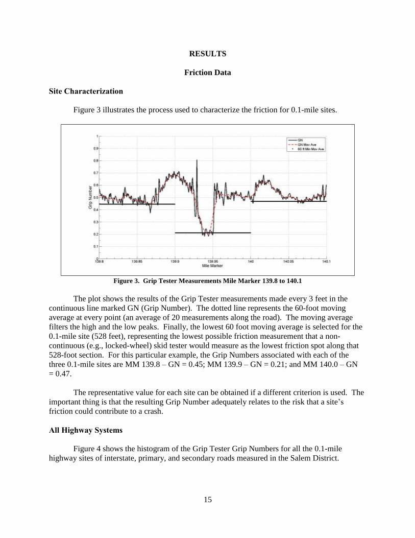
Figure 3 illustrates the process used to characterize the friction for 0.1-mile sites.

Figure 3. Grip Tester Measurements Mile Marker 139.8 to 140.1

The plot shows the results of the Grip Tester measurements made every 3 feet in the

continuous line marked GN (Grip Number). The dotted line represents the 60-foot moving

average at every point (an average of 20 measurements along the road). The moving average

filters the high and the low peaks. Finally, the lowest 60 foot moving average is selected for the

0.1-mile site (528 feet), representing the lowest possible friction measurement that a non-

continuous (e.g., locked-wheel) skid tester would measure as the lowest friction spot along that

528-foot section. For this particular example, the Grip Numbers associated with each of the

three 0.1-mile sites are MM 139.8 – GN = 0.45; MM 139.9 – GN = 0.21; and MM 140.0 – GN

= 0.47.

The representative value for each site can be obtained if a different criterion is used. The

important thing is that the resulting Grip Number adequately relates to the risk that a site’s

friction could contribute to a crash.

All Highway Systems

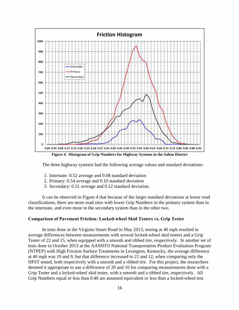
Figure 4 shows the histogram of the Grip Tester Grip Numbers for all the 0.1-mile

highway sites of interstate, primary, and secondary roads measured in the Salem District.

16

Figure 4. Histogram of Grip Numbers for Highway Systems in the Salem District

The three highway systems had the following average values and standard deviations:

1. Interstate: 0.52 average and 0.08 standard deviation

2. Primary: 0.54 average and 0.10 standard deviation

3. Secondary: 0.51 average and 0.12 standard deviation.

It can be observed in Figure 4 that because of the larger standard deviations at lower road

classifications, there are more road sites with lower Grip Numbers in the primary system than in

the interstate, and even more in the secondary system than in the other two.

Comparison of Pavement Friction: Locked-wheel Skid Testers vs. Grip Tester

In tests done at the Virginia Smart Road in May 2013, testing at 40 mph resulted in

average differences between measurements with several locked-wheel skid testers and a Grip

Tester of 22 and 15, when equipped with a smooth and ribbed tire, respectively. In another set of

tests done in October 2013 at the AASHTO National Transportation Product Evaluation Program

(NTPEP) with High Friction Surface Treatments in Lexington, Kentucky, the average difference

at 40 mph was 19 and 9, but that difference increased to 21 and 12, when comparing only the

HFST tested, both respectively with a smooth and a ribbed tire. For this project, the researchers

deemed it appropriate to use a difference of 20 and 10 for comparing measurements done with a

Grip Tester and a locked-wheel skid tester, with a smooth and a ribbed tire, respectively. All

Grip Numbers equal or less than 0.40 are assumed equivalent or less than a locked-wheel test

17

[SN40(S)] of 20 with a smooth tire, which is the current threshold used in Virginia. This is

provided just as a reference comparison that does not affect the results of the analysis because it

is based entirely on the Grip Numbers obtained for all the sections measured.

Crash Data Results

Using the total 8,630 crashes found in each of the three highway systems analyzed in the

Salem District, the following models were developed to predict the cumulative crashes for the

next 3 years.

Regression Model Results

Regression analysis was performed using 3 years of crash data for the three highway

systems. Modification of the negative binomial rates, the intercept term, and the over-dispersion

parameter was performed to generate the regression models, and their goodness-of-fit data are

shown in Tables 4, 5, and 7 that determined the number of significant variables for each model.

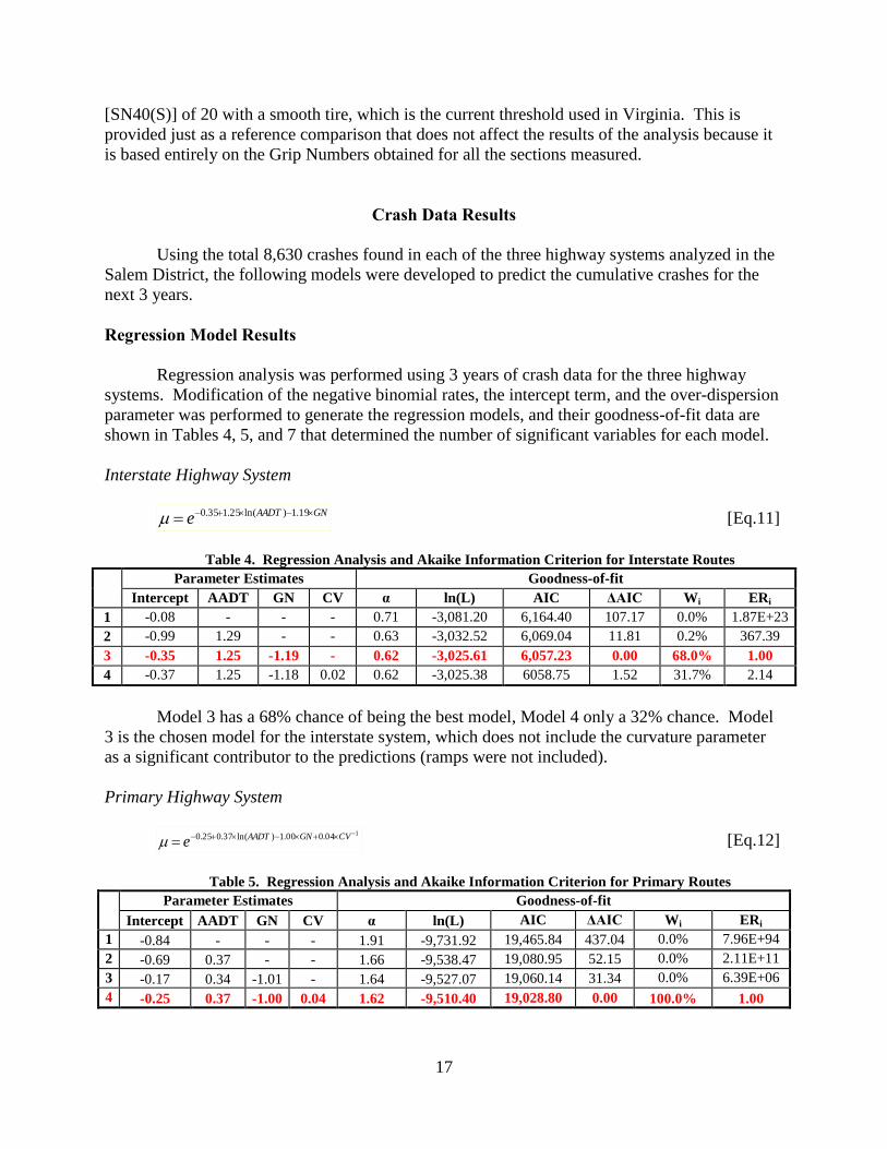
Interstate Highway System

GNAADTe 19.1)ln(25.135.0 [Eq.11]

Table 4. Regression Analysis and Akaike Information Criterion for Interstate Routes

Parameter Estimates Goodness-of-fit

Intercept AADT GN CV α ln(L) AIC ΔAIC Wi ERi

1 -0.08 - - - 0.71 -3,081.20 6,164.40 107.17 0.0% 1.87E+23

2 -0.99 1.29 - - 0.63 -3,032.52 6,069.04 11.81 0.2% 367.39

3 -0.35 1.25 -1.19 - 0.62 -3,025.61 6,057.23 0.00 68.0% 1.00

4 -0.37 1.25 -1.18 0.02 0.62 -3,025.38 6058.75 1.52 31.7% 2.14

Model 3 has a 68% chance of being the best model, Model 4 only a 32% chance. Model

3 is the chosen model for the interstate system, which does not include the curvature parameter

as a significant contributor to the predictions (ramps were not included).

Primary Highway System

104.000.1)ln(37.025.0 CVGNAADTe [Eq.12]

Table 5. Regression Analysis and Akaike Information Criterion for Primary Routes


Intercept AADT GN CV α ln(L) AIC ΔAIC Wi ERi

1 -0.84 - - - 1.91 -9,731.92 19,465.84 437.04 0.0% 7.96E+94

2 -0.69 0.37 - - 1.66 -9,538.47 19,080.95 52.15 0.0% 2.11E+11

3 -0.17 0.34 -1.01 - 1.64 -9,527.07 19,060.14 31.34 0.0% 6.39E+06

4 -0.25 0.37 -1.00 0.04 1.62 -9,510.40 19,028.80 0.00 100.0% 1.00

18

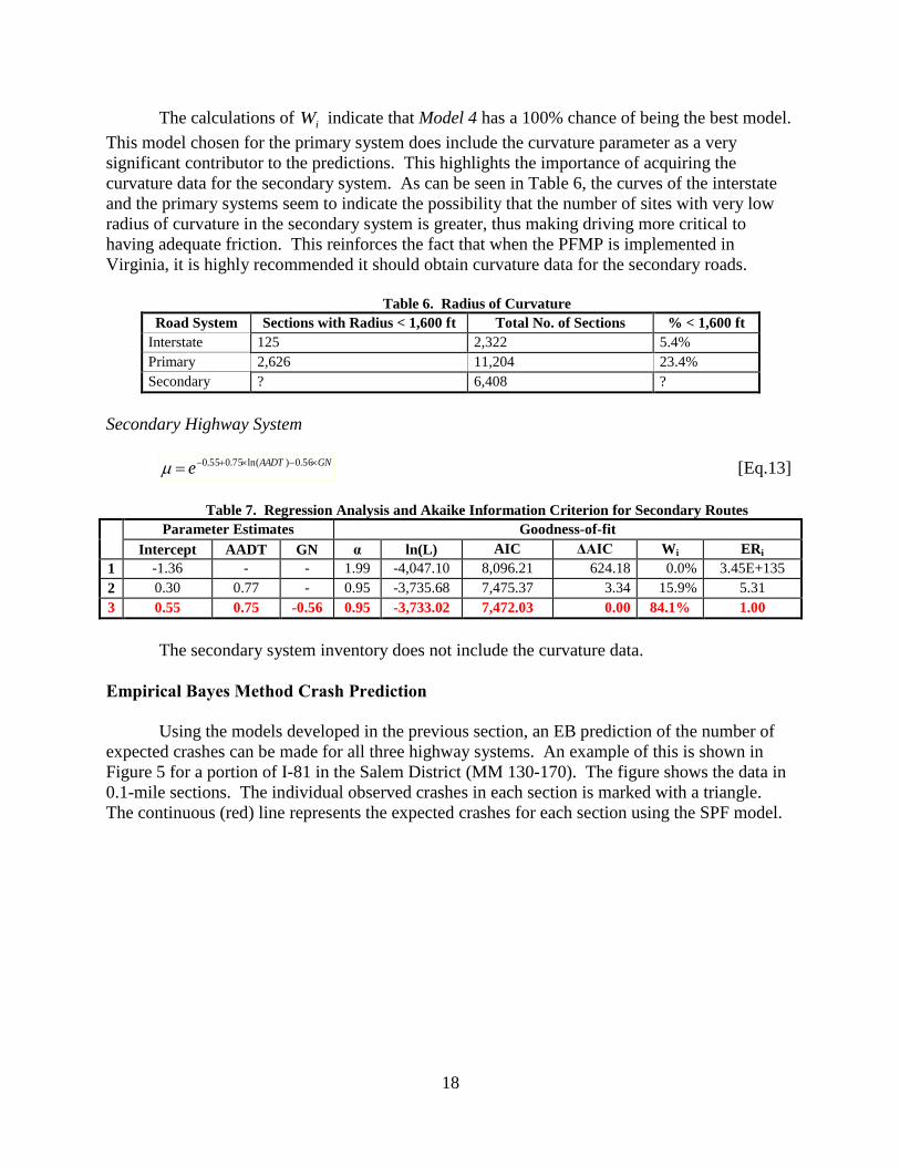
The calculations of iW indicate that Model 4 has a 100% chance of being the best model.

This model chosen for the primary system does include the curvature parameter as a very

significant contributor to the predictions. This highlights the importance of acquiring the

curvature data for the secondary system. As can be seen in Table 6, the curves of the interstate

and the primary systems seem to indicate the possibility that the number of sites with very low

radius of curvature in the secondary system is greater, thus making driving more critical to

having adequate friction. This reinforces the fact that when the PFMP is implemented in

Virginia, it is highly recommended it should obtain curvature data for the secondary roads.

Table 6. Radius of Curvature

Road System Sections with Radius < 1,600 ft Total No. of Sections % < 1,600 ft

Interstate 125 2,322 5.4%

Primary 2,626 11,204 23.4%

Secondary ? 6,408 ?

Secondary Highway System

GNAADTe 56.0)ln(75.055.0 [Eq.13]

Table 7. Regression Analysis and Akaike Information Criterion for Secondary Routes


Intercept AADT GN α ln(L) AIC ΔAIC Wi ERi

1 -1.36 - - 1.99 -4,047.10 8,096.21 624.18 0.0% 3.45E+135

2 0.30 0.77 - 0.95 -3,735.68 7,475.37 3.34 15.9% 5.31

3 0.55 0.75 -0.56 0.95 -3,733.02 7,472.03 0.00 84.1% 1.00

The secondary system inventory does not include the curvature data.

Empirical Bayes Method Crash Prediction

Using the models developed in the previous section, an EB prediction of the number of

expected crashes can be made for all three highway systems. An example of this is shown in

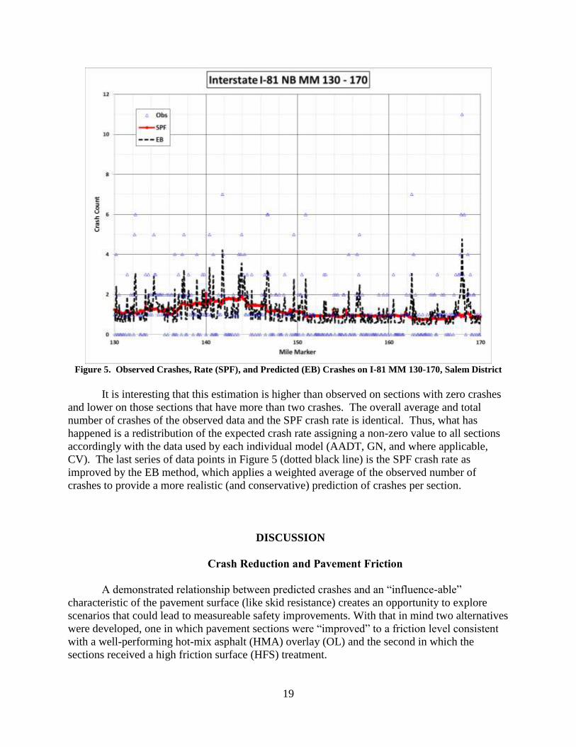
Figure 5 for a portion of I-81 in the Salem District (MM 130-170). The figure shows the data in

0.1-mile sections. The individual observed crashes in each section is marked with a triangle.

The continuous (red) line represents the expected crashes for each section using the SPF model.

19

Figure 5. Observed Crashes, Rate (SPF), and Predicted (EB) Crashes on I-81 MM 130-170, Salem District

It is interesting that this estimation is higher than observed on sections with zero crashes

and lower on those sections that have more than two crashes. The overall average and total

number of crashes of the observed data and the SPF crash rate is identical. Thus, what has

happened is a redistribution of the expected crash rate assigning a non-zero value to all sections

accordingly with the data used by each individual model (AADT, GN, and where applicable,

CV). The last series of data points in Figure 5 (dotted black line) is the SPF crash rate as

improved by the EB method, which applies a weighted average of the observed number of

crashes to provide a more realistic (and conservative) prediction of crashes per section.

DISCUSSION

Crash Reduction and Pavement Friction

A demonstrated relationship between predicted crashes and an “influence-able”

characteristic of the pavement surface (like skid resistance) creates an opportunity to explore

scenarios that could lead to measureable safety improvements. With that in mind two alternatives

were developed, one in which pavement sections were “improved” to a friction level consistent

with a well-performing hot-mix asphalt (HMA) overlay (OL) and the second in which the

sections received a high friction surface (HFS) treatment.

20

Average skid resistance for the two surfaces used in this exercise was based on test

results for different pavements at the Virginia Smart Road, the NTPEP tests mentioned earlier,

and recent measurements made on Virginia interstate pavements in the Salem District. The

average Grip Number (GN) values assumed were 0.70 for OL and 0.95 for HFS. Substituting

these values to represent friction level for a given pavement section, the analysis generates a new

predicted SPF rate (when the observed GN for that specific section is lower than the proposed

GNOL or GNHFS), which we will call OL or HFS , respectively. These rates are then used to make

a new EB estimate by applying a multiplier that is proportionally related to the original i , as

shown in Equations 14 and 15.

i

i

OLOLi

[Eq.14]

i

i

HFSHFSi

[Eq.15]

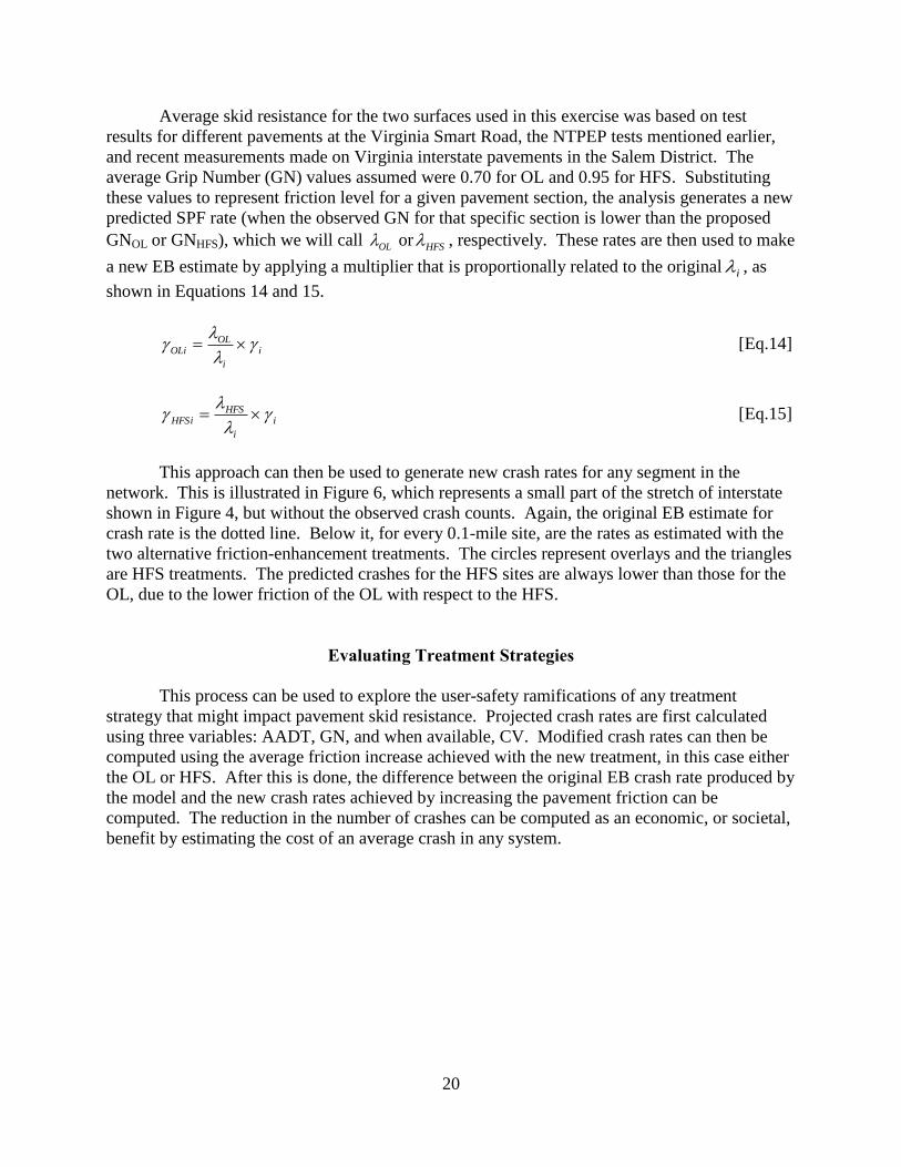
This approach can then be used to generate new crash rates for any segment in the

network. This is illustrated in Figure 6, which represents a small part of the stretch of interstate

shown in Figure 4, but without the observed crash counts. Again, the original EB estimate for

crash rate is the dotted line. Below it, for every 0.1-mile site, are the rates as estimated with the

two alternative friction-enhancement treatments. The circles represent overlays and the triangles

are HFS treatments. The predicted crashes for the HFS sites are always lower than those for the

OL, due to the lower friction of the OL with respect to the HFS.

Evaluating Treatment Strategies

This process can be used to explore the user-safety ramifications of any treatment

strategy that might impact pavement skid resistance. Projected crash rates are first calculated

using three variables: AADT, GN, and when available, CV. Modified crash rates can then be

computed using the average friction increase achieved with the new treatment, in this case either

the OL or HFS. After this is done, the difference between the original EB crash rate produced by

the model and the new crash rates achieved by increasing the pavement friction can be

computed. The reduction in the number of crashes can be computed as an economic, or societal,

benefit by estimating the cost of an average crash in any system.

21

Figure 6. Original EB, EBOL, and EBHFS Crash Rates on I-81 MM 130-170, Salem District

Crash Costs

The average cost of a crash can be complicated to estimate and requires several sources.

The first one is the Guidance on Treatment of the Economic Value of a Statistical Life (VSL) in

the U.S. Department of Transportation Analyses. In its conclusion, the Under Secretary for

Policy recommends “studies published in recent years indicate a VSL of $9.1 million in current

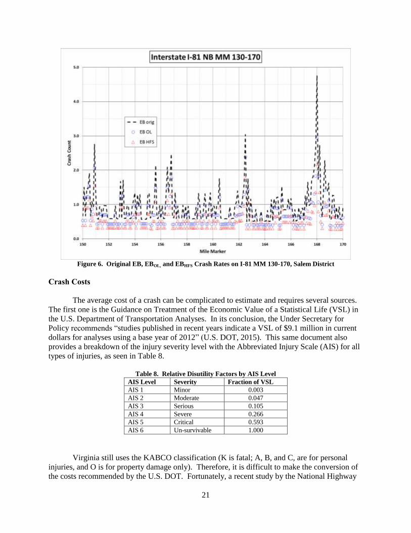
dollars for analyses using a base year of 2012” (U.S. DOT, 2015). This same document also

provides a breakdown of the injury severity level with the Abbreviated Injury Scale (AIS) for all

types of injuries, as seen in Table 8.

Table 8. Relative Disutility Factors by AIS Level

AIS Level Severity Fraction of VSL

AIS 1 Minor 0.003

AIS 2 Moderate 0.047

AIS 3 Serious 0.105

AIS 4 Severe 0.266

AIS 5 Critical 0.593

AIS 6 Un-survivable 1.000

Virginia still uses the KABCO classification (K is fatal; A, B, and C, are for personal

injuries, and O is for property damage only). Therefore, it is difficult to make the conversion of

the costs recommended by the U.S. DOT. Fortunately, a recent study by the National Highway

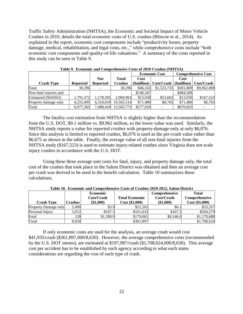
22

Traffic Safety Administration (NHTSA), the Economic and Societal Impact of Motor Vehicle

Crashes in 2010, details the total economic costs of U.S. crashes (Blincoe et al., 2014). As

explained in the report, economic cost components include “productivity losses, property

damage, medical, rehabilitation, and legal costs, etc.,” while comprehensive costs include “both

economic cost components and quality-of-life valuations.” A summary of the costs reported in

this study can be seen in Table 9.

Table 9. Economic and Comprehensive Costs of 2010 Crashes (NHTSA)

Crash Type Reported

Not

Reported

Total

Crashes

Economic Cost Comprehensive Cost

Cost

($million) Cost/Crash

Cost

($million) Cost/Crash

Fatal 30,296 - 30,296 $46,163 $1,523,733 $301,809 $9,962,008

Non-fatal injuries and

1,791,572 1,178,391 2,969,963

$146,347

$53,663

$484,506

$167,523 Uninjured (MAISO) $13,030 $13,030

Property damage only 4,255,495 6,310,019 10,565,514 $71,480 $6,765 $71,480 $6,765

Total 6,077,363 7,488,410 13,565,773 $277,020 - $870,825 -

The fatality cost estimation from NHTSA is slightly higher than the recommendation

from the U.S. DOT, $9.1 million vs. $9.962 million, so the lower value was used. Similarly, the

NHTSA study reports a value for reported crashes with property-damage-only at only $6,076.

Since this analysis is limited to reported crashes, $6,076 is used as the per-crash value rather than

$6,675 as shown in the table. Finally, the average value of all non-fatal injuries from the

NHTSA study ($167,523) is used to estimate injury-related crashes since Virginia does not scale

injury crashes in accordance with the U.S. DOT.

Using these three average unit costs for fatal, injury, and property damage only, the total

cost of the crashes that took place in the Salem District was obtained and then an average cost

per crash was derived to be used in the benefit calculation. Table 10 summarizes these

calculations.

Table 10. Economic and Comprehensive Costs of Crashes 2010-2012, Salem District

Crash Type Crashes

Economic

Cost/Crash

($1,000)

Total Economic

Cost ($1,000)

Comprehensive

Cost/Crash

($1,000)

Total

Comprehensive

Cost ($1,000)

Property Damage only 5,490 $3.9 $21,202 $6.1 $33,357

Personal Injury 3,012 $167.5 $161,633 $167.5 $504,579

Fatal 128 $1,398.9 $179,061 $9,146.0 $1,170,688

Total 8,630 $361,897 $1,708,624

If only economic costs are used for the analysis, an average crash would cost

$41,935/crash ($361,897,000/8,630). However, the average comprehensive costs (recommended

by the U.S. DOT memo), are estimated at $197,987/crash ($1,708,624,000/8,630). This average

cost per accident has to be established by each agency according to what each states

considerations are regarding the cost of each type of crash.

23

Treatment Costs

A recent report detailed average costs for HFS treatments at $27/yd2 and the average cost

of an HMA overlay for a longer section at $10/yd2 (Sprinkel, et al., 2015). That means that these

two treatments for 0.1 mile of road (528 ft), two 12-ft lanes, represent a cost of $14,080 and

$38,016 for an overlay and an HFS treatment, respectively.

Benefit to Cost Analysis

When assessing the benefits from prevented crashes as predicted using the developed

models, it becomes clear very quickly that regardless of the treatment selected ($14,080 or

$38,016 per 0.1-mile section), increasing the friction has a net positive economic effect. A case

study from the Salem District (discussed next) helps demonstrates how pavement friction data

could be incorporated into existing pavement maintenance procedures to improve safety and

reduce overall societal costs.

Case Study 1: I-81 Mile Markers 167-169

The section of I-81 between mile markers 167 and 169 incorporates characteristics that

are conducive for studying measures for improving highway safety. This location, referred to as

the Arcadia Exit, consists of a composite “S” curve with the first curve having a radius of 1,050

ft and the second one a radius of 1,200 ft. Figure 7 shows two plan views of the two curves at

the site.

Figure 7. I-81 Northbound MM 167 to 169, Salem District (from Google maps)

These curves are also located at the bottom of a vertical sag curve, which probably causes

vehicles to be going faster than normal in the entrance to the horizontal curves. The small

radius, the increased speed, and a short tangent between both curves, likely challenge the

effectiveness of the design cross-section, reducing the tolerance for driver error when negotiating

24

the curves. This particular section of road experienced 58 crashes in 2 miles, and in the middle,

from 167.6 to 168.6, there have been 43 crashes in 3 years.

Analysis that contrasts current friction against that which could be achieved using two

possible alternative treatments (i.e., OL and HFS) show a great potential for improvement by

increasing the available friction. This can be seen through the results presented in Table 11.

Table 11. EB Analysis Results for I-81 MM 167-169 With OL and HFS Alternatives

MP

Obs.

Crashes GN

AADT

(10,000)

ln

(AADT)

CV

(mi)

Inv.

CV

SPF Model (Eq.

11) OL

OL

Improve

HFS

HFS

Improve Rate Weight EB Rate EB Rate EB

167.0 1 0.41 1.7 0.53 0.38 2.67 0.843 0.653 0.551 0.596 0.389 0.16 0.442 0.289 0.26

167.1 2 0.39 1.7 0.53 0.38 2.67 0.867 0.647 1.267 0.596 0.870 0.40 0.442 0.646 0.62

167.2 1 0.37 1.7 0.53 0.38 2.67 0.878 0.644 0.921 0.596 0.625 0.30 0.442 0.464 0.46

167.3 3 0.36 1.7 0.53 0.38 2.67 0.895 0.640 1.654 0.596 1.100 0.55 0.442 0.817 0.84

167.4 1 0.30 1.7 0.53 0.71 1.40 0.958 0.624 0.974 0.596 0.605 0.37 0.442 0.449 0.52

167.5 1 0.24 1.7 0.53 0.71 1.40 1.033 0.606 1.020 0.596 0.588 0.43 0.442 0.437 0.58

167.6 3 0.29 1.7 0.53 0.71 1.40 0.968 0.621 1.737 0.596 1.069 0.67 0.442 0.794 0.94

167.7 3 0.24 1.7 0.53 0.71 1.40 1.036 0.605 1.811 0.596 1.041 0.77 0.442 0.773 1.04

167.8 4 0.31 1.7 0.53 10.00 0.10 0.950 0.626 2.091 0.596 1.311 0.78 0.442 0.973 1.12

167.9 6 0.37 1.7 0.53 1.80 0.56 0.878 0.644 2.702 0.596 1.832 0.87 0.442 1.360 1.34

168.0 11 0.29 1.7 0.53 1.80 0.56 0.968 0.621 4.766 0.596 2.932 1.83 0.442 2.177 2.59

168.1 3 0.29 1.7 0.53 1.80 0.56 0.969 0.621 1.738 0.596 1.069 0.67 0.442 0.793 0.94

168.2 6 0.36 1.7 0.53 1.80 0.56 0.891 0.641 2.727 0.596 1.822 0.91 0.442 1.353 1.37

168.3 1 0.36 1.9 0.64 1.80 0.56 1.021 0.609 1.013 0.684 0.679 0.33 0.508 0.504 0.51

168.4 0 0.36 1.9 0.64 3.03 0.33 1.032 0.606 0.625 0.684 0.415 0.21 0.508 0.308 0.32

168.5 2 0.34 1.9 0.64 3.03 0.33 1.050 0.602 1.428 0.684 0.931 0.50 0.508 0.691 0.74

168.6 4 0.31 1.9 0.64 0.95 1.05 1.093 0.592 2.278 0.684 1.426 0.85 0.508 1.058 1.22

168.7 2 0.36 1.9 0.64 0.95 1.05 1.028 0.607 1.410 0.684 0.938 0.47 0.508 0.697 0.71

168.8 2 0.38 1.9 0.64 0.33 2.99 1.000 0.614 1.386 0.684 0.948 0.44 0.508 0.704 0.68

168.9 3 0.38 1.7 0.53 0.20 4.95 0.869 0.646 1.622 0.596 1.112 0.51 0.442 0.826 0.80

169.0 0 0.40 1.7 0.53 0.20 4.95 0.852 0.651 0.555 0.596 0.388 0.17 0.442 0.288 0.27

SPF Model “Eq. 11” = predicted crash rates (crashes every 3 years) with current friction.

OL EB = predicted crash rates with Overlay (OL).

HFS EB = predicted crash rates with high friction surface (HFS).

OL Improve = reduction in predicted crashes with OL.

HFS Improve = reduction in predicted crashes with HFS.

From this table, the EB model predicts that the total improvement in the “critical mile”

(from MM 167.6 to MM 168.6, shaded) containing both curves and the short tangent in between

could have an expected reduction of 8.4 crashes (every 3 years) if it is overlaid (OL) and 12.1

crashes should an HFS treatment be applied.

To calculate which treatment would be better, a benefit/cost (B/C) comparison or a total

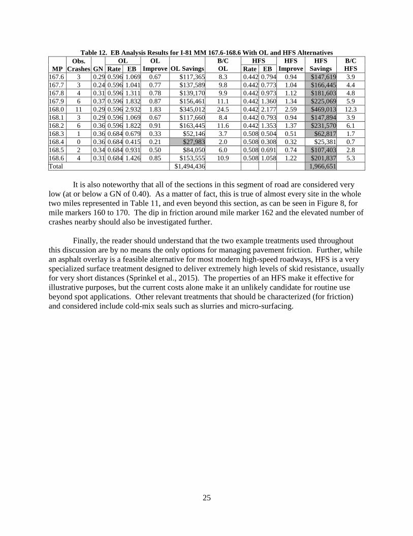
comprehensive economic savings can be made for each site, as shown in Table 12. This analysis

reflects a cost for each 0.1 mile of $14,080 for an overlay (OL), $38,016 for the HFS treatment,

and $197,987 for each crash avoided with the new treatment. It is interesting to note that

although the B/C ratio for installing the conventional overlay (OL) is higher, the total

comprehensive savings for the “critical mile” section is almost a half-million dollars more with

the HFS treatment.

25

Table 12. EB Analysis Results for I-81 MM 167.6-168.6 With OL and HFS Alternatives

MP

Obs.

Crashes GN

OL OL

Improve

OL Savings

B/C

OL

HFS HFS

Improve

HFS

Savings

B/C

HFS Rate EB Rate EB

167.6 3 0.29 0.596 1.069 0.67 $117,365 8.3 0.442 0.794 0.94 $147,619 3.9

167.7 3 0.24 0.596 1.041 0.77 $137,589 9.8 0.442 0.773 1.04 $166,445 4.4

167.8 4 0.31 0.596 1.311 0.78 $139,170 9.9 0.442 0.973 1.12 $181,603 4.8

167.9 6 0.37 0.596 1.832 0.87 $156,461 11.1 0.442 1.360 1.34 $225,069 5.9

168.0 11 0.29 0.596 2.932 1.83 $345,012 24.5 0.442 2.177 2.59 $469,013 12.3

168.1 3 0.29 0.596 1.069 0.67 $117,660 8.4 0.442 0.793 0.94 $147,894 3.9

168.2 6 0.36 0.596 1.822 0.91 $163,445 11.6 0.442 1.353 1.37 $231,570 6.1

168.3 1 0.36 0.684 0.679 0.33 $52,146 3.7 0.508 0.504 0.51 $62,817 1.7

168.4 0 0.36 0.684 0.415 0.21 $27,983 2.0 0.508 0.308 0.32 $25,381 0.7

168.5 2 0.34 0.684 0.931 0.50 $84,050 6.0 0.508 0.691 0.74 $107,403 2.8

168.6 4 0.31 0.684 1.426 0.85 $153,555 10.9 0.508 1.058 1.22 $201,837 5.3

Total $1,494,436 1,966,651

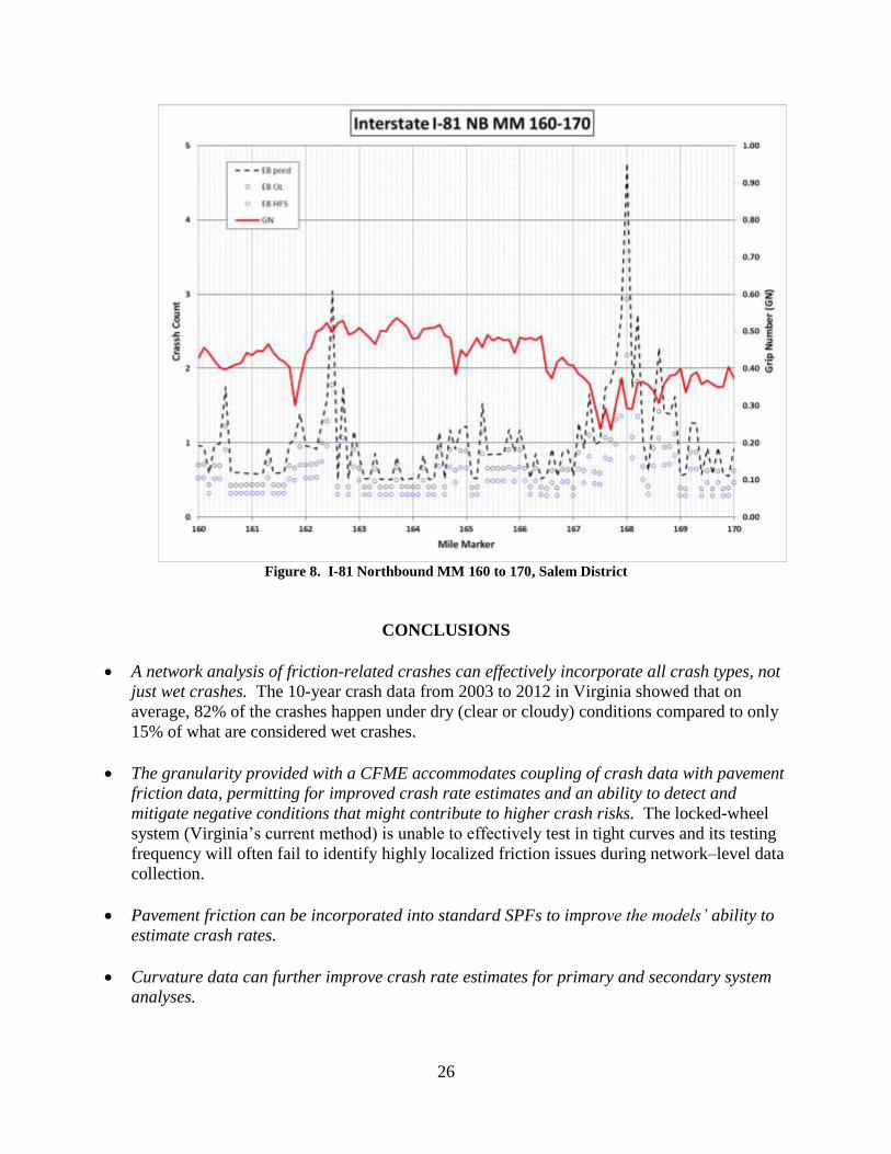
It is also noteworthy that all of the sections in this segment of road are considered very

low (at or below a GN of 0.40). As a matter of fact, this is true of almost every site in the whole

two miles represented in Table 11, and even beyond this section, as can be seen in Figure 8, for

mile markers 160 to 170. The dip in friction around mile marker 162 and the elevated number of

crashes nearby should also be investigated further.

Finally, the reader should understand that the two example treatments used throughout

this discussion are by no means the only options for managing pavement friction. Further, while

an asphalt overlay is a feasible alternative for most modern high-speed roadways, HFS is a very

specialized surface treatment designed to deliver extremely high levels of skid resistance, usually

for very short distances (Sprinkel et al., 2015). The properties of an HFS make it effective for

illustrative purposes, but the current costs alone make it an unlikely candidate for routine use

beyond spot applications. Other relevant treatments that should be characterized (for friction)

and considered include cold-mix seals such as slurries and micro-surfacing.

26

Figure 8. I-81 Northbound MM 160 to 170, Salem District

CONCLUSIONS

A network analysis of friction-related crashes can effectively incorporate all crash types, not

just wet crashes. The 10-year crash data from 2003 to 2012 in Virginia showed that on

average, 82% of the crashes happen under dry (clear or cloudy) conditions compared to only

15% of what are considered wet crashes.

The granularity provided with a CFME accommodates coupling of crash data with pavement

friction data, permitting for improved crash rate estimates and an ability to detect and

mitigate negative conditions that might contribute to higher crash risks. The locked-wheel

system (Virginia’s current method) is unable to effectively test in tight curves and its testing

frequency will often fail to identify highly localized friction issues during network–level data

collection.

Pavement friction can be incorporated into standard SPFs to improve the models’ ability to

estimate crash rates.

Curvature data can further improve crash rate estimates for primary and secondary system

analyses.

27

Comprehensive crash costs can be used with improved SPFs to perform benefit/cost analyses

that consider alternative friction repair treatments.

The total economic savings from crash cost avoidance through friction enhancement can be

considerable. An example trade-off analysis resulted in high benefit-to-cost ratios when

addressing low friction with two alternative treatments. The highest comprehensive crash

cost savings were realized with an application of HFS treatments.

RECOMMENDATIONS

1. VDOT’s materials and traffic safety engineers should expand the use of continuous friction

measurement equipment (CFME) to monitor pavement skid resistance. Appendix B provides

some logistical information and economic analysis that may help VDOT in considering

options for equipment to manage pavement friction moving forward.

2. VDOT’s safety and maintenance engineers should seek to incorporate pavement friction in

SPFs to improve network crash rate predictions. This analysis should include all crash types

(wet and non-wet) and, when available, should incorporate horizontal curvature.

3. VTRC should work with VTTI to use pavement macrotexture, cross-section, grade, and

horizontal curvature to improve crash rate estimates. This research should attempt to take

maximum advantage of VTTI’s research with the FHWA to deploy pilot Pavement Friction

Management Programs (PFPMs) using a Sideway-force Coefficient Routine Investigation

Machine (SCRIM).

4. VDOT’s traffic safety and maintenance engineers should prepare to use improved SPFs (that

incorporate friction and other pavement surface and geometric properties) to develop

proactive and cost-effective friction repair treatment plans. The demonstrated methodology

uses estimated crash rates to predict comprehensive crash costs. Estimated crash costs for in-

service conditions can be contrasted against “repaired” costs (when warranted) to maximize

benefit-to-cost for treatments and/or minimize overall crash costs.

BENEFITS AND IMPLEMENTATION

Benefits

The added predictive power of friction in the current VDOT SPF model proved

significant in estimating crash occurrences. To further illustrate the value of these modified SPF

models, a benefit analysis was conducted for all sections of the three highway systems in the

Salem District for which the B/C ratio for friction repair was greater than 1.0. The results are

presented in Table 13.

28

Table 13. Results with OL and HFS Alternatives on Highway Systems in the Salem District

System Crashes % Sections % Benefits ($1,000) Costs ($1,000) Savings ($1,000)

Interstate 2,141 2,322

OL reduction 337 16% 1,202 52% $66,712 $16,924 $49,788

HFS reduction 513 24% 836 36% $101,634 $31,781 $69,853

Primary 4,844 11,204

OL reduction 384 8% 1,443 13% $76,124 $20,317 $55,807

HFS reduction 512 11% 820 7% $101,439 $31,173 $70,266

Secondary 1,645 6,408

OL reduction 40 2% 151 2% $7,851 $2,126 $5,725

HFS reduction 40 2% 62 1% $7,794 $2,356 $5,437

Total 8,630 19,934

OL reduction 761 9% 2,796 14% $150,689 $39,367 $111,322

HFS reduction 1,065 12% 1,718 9% $210,869 $65,311 $145,557

Using these improved SPFs, the higher the friction, the fewer the expected crashes.

When a conventional plant-mix overlay (OL) is used, the analysis predicts 761 fewer crashes.

When an HFS is used, the analysis expects to reduce crashes by 1,065. The majority of the

comprehensive savings is achieved on the interstate and primary systems, but regardless of the

treatment chosen, the net economic benefit (societal savings) for one VDOT district could be in

excess of $100 million every 3 years. Total economic savings of this magnitude would easily

offset the costs of a comprehensive PFMP, the equipment necessary to administer it, the

construction of the treatments on high volume roads, and even significant skid-crash mitigation

on those sites for which traffic volumes would ordinarily be too low to meet strict economic

criteria (such as low-volume high-risk rural roads, HRRR).

This research ultimately improves the ability of the district maintenance and regional

traffic engineers to match user demands for pavement friction with the capability of common

surface alternatives, both on a local and system-wide basis. An effective PFMP better positions

VDOT to respond to its FY15-16 Business Plan, Section 3.2.3., which includes a focus on

“lowering the number of deaths and severe crashes through engineered safety improvements.”

Implementation

Implementation will next involve collecting continuous data on Virginia’s Corridors of

Statewide Significance (CSS), a joint activity with VDOT, FHWA, and VTTI. This effort will

include about 3,700 centerline miles of highway; 1,100 miles of divided interstate; and

approximately 2,600 miles of divided and four-lane undivided primary routes (see Figure 9). In

addition to friction and curvature, the analysis of the CSS data will also incorporate texture,

cross-slope, and grade. The preliminary cost is estimated to be around $200,000; and the effort

is expected to consume about 1 year.

29

Figure 9. Corridors of Statewide Significance (VTrans 2035)

ACKNOWLEDGMENTS

The research team acknowledges the significant contribution of the project panel

members throughout the development of the project. Their guidance and feedback were

instrumental for the completion of the project. Personnel from VDOT’s TED were instrumental

in providing the crash and other data sets that were needed for the execution of the project. The

team thanks the operators that collected all of the friction field data: William Hobbs, Kenneth

Smith, and Robert Honeywell. The team also acknowledges the significant contributions of the

various state and federal members of the various meetings that have had a chance to review and

give their opinions on the development of this work, especially those involved in the FHWA-

funded research project “Development and Demonstration of Pavement Friction Management

Programs.”

REFERENCES

AASHTO. Highway Safety Manual. Washington, DC, 2008.

AASHTO. Elements of Design. In A Policy on Geometric Design of Highways and Streets, 6th

Edition. Washington, DC, 2011.

Blincoe, L., Miller, T., Zaloshnja, E., and Lawrence, B. The Economic and Societal Impact of

Motor Vehicle Crashes, 2010. U.S. DOT, National Highway Traffic Safety

Administration, Washington, DC, 2014.

Cameron, A.C., and Trivedi, P.K. Chapter 17: Count-Data Models. In Microeconometrics

Using Stata, Revised Edition. Stata Press, College Station, TX, 2010, pp. 567-613.

30

Chowdhury, T. Pavement Condition Data: Locally Maintained Roads.

http://www.virginiadot.org/business/resources/local_assistance/Pavement-Data-

Arterials.pdf. Accessed March 12, 2015.

Commonwealth of Virginia, Department of Motor Vehicles, Virginia Highway Safety Office,

Virginia Traffic Crash Facts.

http://www.dmv.virginia.gov/safety/#crash_data/crash_facts/index.asp. Accessed

February 2, 2014.

Federal Highway Administration. Pavement Friction Management. Technical Advisory T

5040.38. Washington, DC, 2010.

Federal Highway Administration. Title 23, Section 148, U.S. Code, including amendments made

by SAFETEA-LU. http://www.fhwa.dot.gov/safetealu/legis.htm. Accessed February

2013a.

Federal Highway Administration. Highway Safety Improvement Program (HSIP).

http://www.fhwa.dot.gov/map21/hsip.cfm. Accessed February 2013b.

Flintsch, G., and de León Izeppi, E. Virginia Tech Transportation Institute, Equipment

Recommendation Report, Development and Demonstration of Pavement Friction

Management Programs, FHWA DTFH61-09-R-00035, 2011.

Flintsch, G., de León Izeppi, E., McGhee, K., and Najafi, S. Speed Adjustment Factors for

Locked-Wheel Skid Trailer Measurements. In Transportation Research Record: Journal

of the Transportation Research Board, No. 2155. Transportation Research Board of the

National Academies, Washington, DC, 2010, pp. 117–123.

Habib, A. Friction Testing Program in Virginia. Presented at the 7th Symposium on Pavement

Surface Characteristics (SURF) of the World Road Association in Norfolk, Virginia,

September 2012.

Hauer, E. Overdispersion in Modelling Accidents on Road Sections and in Empirical Bayes

Estimation. Accident Analysis & Prevention, Vol. 33, No. 6, November 2001, pp. 801-

808.

Kweon, Y.-J., and Lim, I.-K. Development of Safety Performance Functions for Multilane

Highway and Freeway Segments Maintained by the Virginia Department of

Transportation. FHWA/VCTIR 14-R14. Virginia Center for Transportation Innovation

and Research, Charlottesville, 2014.

Lord, D., and Park, B.-J. Appendix D: Negative Binomial Regression Models and Estimation

Methods. In CrimeStat Version 3.3 Update Notes: Part 2: Regression Modeling. The

National Institute of Justice, Washington, DC, 2010.

http://www.virginiadot.org/business/resources/local_assistance/Pavement-Data-Arterials.pdf

http://www.virginiadot.org/business/resources/local_assistance/Pavement-Data-Arterials.pdf

http://www.dmv.virginia.gov/safety/#crash_data/crash_facts/index.asp

31

Mahone, D., and Sherwood, W.C. Virginia’s Wet Accident Reduction Program: A User’s

Manual. Virginia Transportation Research Council, Charlottesville, 1996.

Mazerolle, M.J. APPENDIX 1: Making Sense out of Akaike’s Information Criterion (AIC): Its

Use and Interpretation in Model Selection and Inference from Ecological Data. In

Mouvements et reproduction des amphibians en tourbières perturbées. Université Laval,

Québec, Canada, 2004.

McCarthy, R. Performing Network-Level Crash Evaluation Using Skid Resistance. Master’s

Thesis, Virginia Polytechnic Institute and State University, Blacksburg, 2015.

McGovern, C., Rusch, P., and Noyce, D. State Practices to Reduce Wet Weather Skidding

Crashes. FHWA-SA-11-21. Federal Highway Administration, Office of Safety,

Washington, DC, 2011.

Peck, R.B. Advantages and Limitations of the Observational Method in Applied Soil

Mechanics. Géotechnique, Vol. 69, 1969, pp. 171-187.

http://www.icevirtuallibrary.com/content/article/10.1680/geot.1969.19.2.171.

Sprinkel, M., McGhee, K., and de León Izeppi, E. Virginia’s Experience with High Friction

Surface Treatments. Paper presented at the 94th Annual Meeting of the Transportation

Research Board. Accepted for publication, 2015.

Srinivasan, R., and Bauer, K. Safety Performance Function Development Guide: Developing

Jurisdiction-Specific SPFs. FHWA-SA-14-005. Federal Highway Administration,

Office of Safety, Washington, DC, 2013.

U.S. Department of Transportation. Toward Zero Deaths: A National Strategy on Highway

Safety. http://safety.transportation.org/. Accessed February 2013.

U.S. Department of Transportation. Economic Values Used in Analysis.

http://www.dot.gov/regulations/economic-values-used-in-analysis. Accessed April 2015.

Virginia Center for Transportation Innovation and Research. About VCTIR: History.

http://vtrc.virginiadot.org/DynamicPage.aspx?PageId=34. Accessed January 24, 2013.

Virginia Department of Transportation. 2007 Wet Accident Reduction Program Report. 2009.

http://www.virginiadot.org/business/resources/Materials/2007_WARP_Report.pdf.

Accessed February 2013.

Virginia Department of Transportation, Virginia Surface Transportation Safety Executive

Committee, Commonwealth of Virginia’s Strategic Highway Safety Plan 2006-2010.

http://www.virginiadot.org/info/hwysafetyplan.asp. Accessed February 2013.

Virginia Department of Transportation. State of the Pavement Reports.

http://www.virginiadot.org/info/state_of_the_pavement.asp. Accessed February 2, 2014.

http://www.icevirtuallibrary.com/content/article/10.1680/geot.1969.19.2.171

http://www.dot.gov/regulations/economic-values-used-in-analysis

http://www.virginiadot.org/business/resources/Materials/2007_WARP_Report.pdf

http://www.virginiadot.org/info/state_of_the_pavement.asp

32

Virginia Department of Transportation. Virginia’s Highway System.

http://www.virginiadot.org/about/vdot_hgwy_sys.asp. Accessed March 12, 2015.

Whitehurst, E.A., updated by Henry, J. J. Committee E-17 on Vehicle-Pavement Systems, a Fifty

Year History 1960-2010. ASTM Committee E-17, January 5, 2011.

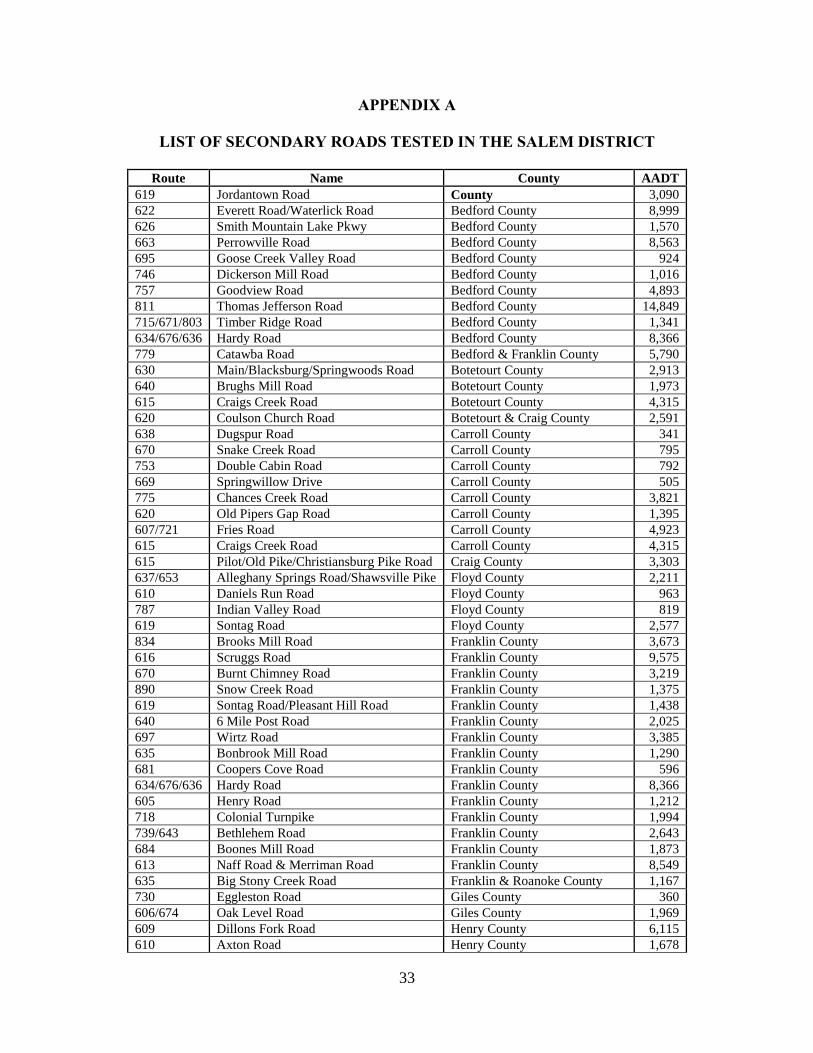
http://www.virginiadot.org/about/vdot_hgwy_sys.asp

33

APPENDIX A

LIST OF SECONDARY ROADS TESTED IN THE SALEM DISTRICT

Route Name County AADT

619 Jordantown Road County 3,090

622 Everett Road/Waterlick Road Bedford County 8,999

626 Smith Mountain Lake Pkwy Bedford County 1,570

663 Perrowville Road Bedford County 8,563

695 Goose Creek Valley Road Bedford County 924

746 Dickerson Mill Road Bedford County 1,016

757 Goodview Road Bedford County 4,893

811 Thomas Jefferson Road Bedford County 14,849

715/671/803 Timber Ridge Road Bedford County 1,341

634/676/636 Hardy Road Bedford County 8,366

779 Catawba Road Bedford & Franklin County 5,790

630 Main/Blacksburg/Springwoods Road Botetourt County 2,913

640 Brughs Mill Road Botetourt County 1,973

615 Craigs Creek Road Botetourt County 4,315

620 Coulson Church Road Botetourt & Craig County 2,591

638 Dugspur Road Carroll County 341

670 Snake Creek Road Carroll County 795

753 Double Cabin Road Carroll County 792

669 Springwillow Drive Carroll County 505

775 Chances Creek Road Carroll County 3,821

620 Old Pipers Gap Road Carroll County 1,395

607/721 Fries Road Carroll County 4,923

615 Craigs Creek Road Carroll County 4,315

615 Pilot/Old Pike/Christiansburg Pike Road Craig County 3,303

637/653 Alleghany Springs Road/Shawsville Pike Floyd County 2,211

610 Daniels Run Road Floyd County 963

787 Indian Valley Road Floyd County 819

619 Sontag Road Floyd County 2,577

834 Brooks Mill Road Franklin County 3,673

616 Scruggs Road Franklin County 9,575

670 Burnt Chimney Road Franklin County 3,219

890 Snow Creek Road Franklin County 1,375

619 Sontag Road/Pleasant Hill Road Franklin County 1,438

640 6 Mile Post Road Franklin County 2,025

697 Wirtz Road Franklin County 3,385

635 Bonbrook Mill Road Franklin County 1,290

681 Coopers Cove Road Franklin County 596

634/676/636 Hardy Road Franklin County 8,366

605 Henry Road Franklin County 1,212

718 Colonial Turnpike Franklin County 1,994

739/643 Bethlehem Road Franklin County 2,643

684 Boones Mill Road Franklin County 1,873

613 Naff Road & Merriman Road Franklin County 8,549

635 Big Stony Creek Road Franklin & Roanoke County 1,167

730 Eggleston Road Giles County 360

606/674 Oak Level Road Giles County 1,969

609 Dillons Fork Road Henry County 6,115

610 Axton Road Henry County 1,678

34

620 Old Liberty Road Henry County 2,015

650 Irisburg Road Henry County 5,241

687 Preston Road/Stones Dairy Road Henry County 4,095

698 Blackberry Road Henry County 3,243

692 Horsepasture Price Road Henry County 1,861

687 Soapstone Road Henry County 1,241

605 Henry Road Henry County 1,211

603 North Fork Road/Den Hill Road Henry & Franklin County 2,362

685 Prices Fork Road Montgomery County 9,890

615 Pilot/Old Pike/Christiansburg Pike Road Montgomery County 3,303

637/653 Alleghany Springs Road/Shawsville Pike Montgomery & Floyd County 2,211

622 Bradshaw Road Montgomery & Floyd County 1,819

624 Mount Tabor Road/Newport Road Montgomery & Roanoke County 972

785 Blacksburg Road Montgomery & Roanoke County 554

614 Squirrel Spur Road Montgomery & Roanoke County 413

626 Abram Penn Hwy Patrick County 491

653 Ayers Church Road Patrick County 1,071

773 Ararat Road Patrick County 1,639

680 Spring Road Patrick County 1,951

693 Lead Mine Road Patrick County 1,084

738 Robinson Tract Road Pulaski County 1,059

672 Lowmans Ferry Road Pulaski County 2,320

613 Naff Road & Merriman Road Pulaski County 8,549

622 Bradshaw Road Roanoke County 1,819

624 Mount Tabor Road/Newport Road Roanoke County 972

785 Blacksburg Road Roanoke County 554

720 Colonial Ave Roanoke County 11,117

904 Starkey Road Roanoke County 10,835

679 Buck Mountain Road Roanoke County 6,957

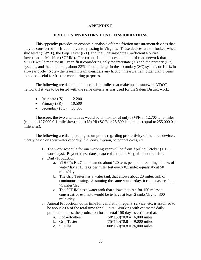
35

APPENDIX B

FRICTION INVENTORY COST CONSIDERATIONS

This appendix provides an economic analysis of three friction measurement devices that

may be considered for friction inventory testing in Virginia. These devices are the locked-wheel

skid tester (LWST), the Grip Tester (GT), and the Sideway-force Coefficient Routine

Investigation Machine (SCRIM). The comparison includes the miles of road network that

VDOT would monitor in 1 year, first considering only the interstate (IS) and the primary (PR)

systems, and then including about 33% of the mileage in the secondary (SC) system, or 100% in

a 3-year cycle. Note - the research team considers any friction measurement older than 3 years

to not be useful for friction monitoring purposes.

The following are the total number of lane-miles that make up the statewide VDOT

network if it was to be tested with the same criteria as was used for the Salem District work:

Interstate (IS) 2,200

Primary (PR) 10,500

Secondary (SC) 38,500

Therefore, the two alternatives would be to monitor a) only IS+PR or 12,700 lane-miles

(equal to 127,000 0.1-mile sites) and b) IS+PR+SC/3 or 25,500 lane-miles (equal to 255,000 0.1-

mile sites).

The following are the operating assumptions regarding productivity of the three devices,

mostly based on their water capacity, fuel consumption, personnel costs, etc.

1. The work schedule for one working year will be from April to October (± 150

workdays). Beyond these dates, data collection in Virginia is not reliable.

2. Daily Production:

a. VDOT’s E-274 unit can do about 120 tests per tank; assuming 4 tanks of

water/day at 10 tests per mile (test every 0.1 mile) equals about 50

miles/day.

b. The Grip Tester has a water tank that allows about 20 miles/tank of

continuous testing. Assuming the same 4 tanks/day, it can measure about

75 miles/day.

c. The SCRIM has a water tank that allows it to run for 150 miles; a

conservative estimate would be to have at least 2 tanks/day for 300

miles/day.

3. Annual Production; down time for calibration, repairs, service, etc. is assumed to

be about 20% of the total time for all units. Working with estimated daily

production rates, the production for the total 150 days is estimated at:

a. Locked-wheel (50*150)*0.8 = 6,000 miles

b. Grip Tester (75*150)*0.8 = 9,000 miles

c. SCRIM (300*150)*0.8 = 36,000 miles

36

4. Both the Locked-wheel and the Grip Tester will be operated by a single

driver/operator, while the SCRIM requires both a driver and an operator.

5. Per diems and hotels expenses are estimated to be an average of $300/week and

$400/week, respectively, for the operators and drivers.

6. The equipment costs for all three devices are estimated here. Caution is to be

taken when comparing them because the prices for the locked-wheel and the Grip

Tester do not represent a unit with a macrotexture laser and the inertial

differential GPS system capable of measuring the cross-slope, grade, and

curvature of the roads, and the price of the trucks that haul them is also not

included.

a. Locked-wheel $150,000 (Tow vehicle not included)

b. Grip Tester $ 80,000 (Tow vehicle not included)

c. SCRIM $800,000

7. All the devices are assumed to have a service life of 10 years for depreciation

purposes and another 10% yearly maintenance cost is assumed during its life.

8. Fuel mileage is assumed to be 10 miles/gallon for the trucks towing both the

locked-wheel and the Grip Tester and only 5 miles/gallon for the SCRIM truck.

With these estimations, an estimate of the overall direct costs, the cost per mile, and the

necessary number of units for each type of device is presented in Table B1.

Table B1. Direct Costs, Cost per Mile and Number of Units Needed for Two Network Scenarios

Road Network Miles ASTM E-274 GT SCRIM

Interstate and Primary 12,700 $200,942 $115,899 $110,725

Units needed 2.1 1.4 0.4

Interstate, Primary, and 33% of Secondary 25,500 $403,467 $232,711 $222,322

Units needed 4.3 2.8 0.7

Direct Costs/mile $15.82 $9.13 $8.72

Estimated production/device/year 6,000 9,000 36,000

These numbers show that for the basic road network package of interstate and primary

network, it would require the operation of 2.1 locked-wheel skid testers, 1.4 Grip Testers, or 0.4

SCRIM units. For the expanded network, including an additional 33% of the secondary roads,

these requirements increase to 4.3 LWST, 2.8 GT, and 0.7 SCRIM. Although careful

consideration should be given to all the assumptions and results, the evidence as presented

appears to favor the SCRIM device, which is consistent with findings from the FHWA study

(Flintsch and de León Izeppi, 2011). It should also be noted that, if desired, the additional cost

for collecting the macrotexture, cross-slope, grade, and curvature data would have to be added to

the total costs of each option for the LWST and the GT, respectively, as well as the consideration

for the cost of the towing vehicle. It is also pertinent to point out that the GT is unproven as a

tool for network testing on this scale.

This analysis (see Table B2) is relevant, regardless of whether VDOT would perform the

services in-house or contract for them as is the case with the distress data that is collected for the

PMS. It is very possible that with direct communication from VDOT, FHWA would be willing

to include VDOT as the fifth state in its demonstration program to manage pavement friction

using the SCRIM device. Table B2. Detailed Cost Analysis Spreadsheet

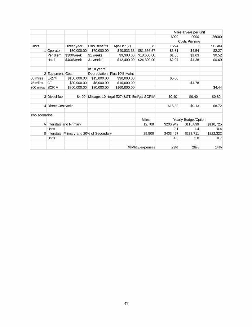
37

6000 9000 36000

Costs Direct/year Plus Benefits Apr-Oct (7) x2 E274 GT SCRIM

1 Operator $50,000.00 $70,000.00 $40,833.33 $81,666.67 $6.81 $4.54 $2.27

Per diem $300/week 31 weeks $9,300.00 $18,600.00 $1.55 $1.03 $0.52

Hotel $400/week 31 weeks $12,400.00 $24,800.00 $2.07 $1.38 $0.69

In 10 years

2 Equipment Cost Depreciation Plus 10% Maint

50 miles E-274 $150,000.00 $15,000.00 $30,000.00 $5.00

75 miles GT $80,000.00 $8,000.00 $16,000.00 $1.78

300 miles SCRIM $800,000.00 $80,000.00 $160,000.00 $4.44

3 Diesel fuel $4.00 Mileage: 10mi/gal E274&GT; 5mi/gal SCRIM $0.40 $0.40 $0.80

4 Direct Costs/mile $15.82 $9.13 $8.72

Two scenarios

Miles

A Interstate and Primary 12,700 $200,942 $115,899 $110,725

Units 2.1 1.4 0.4

B Interstate, Primary and 20% of Secondary 25,500 $403,467 $232,711 $222,322

Units 4.3 2.8 0.7

%MI&E-expenses 23% 26% 14%

Miles a year per unit

Costs Per mile

Yearly Budget/Option

continuous friction measurement equipment as a tool … · continuous friction measurement...

Documents