ORIGINAL PAPER

Continuous detection of weak sensory signals in afferent spike trains:the role of anti-correlated interspike intervals in detection performance

Received: 28 February 2003 / Revised: 20 June 2003 / Accepted: 2 July 2003 / Published online: 14 August 2003� Springer-Verlag 2003

Abstract An important problem in sensory processing isdeciding whether fluctuating neural activity encodes astimulus or is due to variability in baseline activity.Neurons that subserve detection must examine incomingspike trains continuously, and quickly and reliablydifferentiate signals from baseline activity. Here wedemonstrate that a neural integrator can perform con-tinuous signal detection, with performance exceedingthat of trial-based procedures, where spike counts insignal- and baseline windows are compared. The pro-cedure was applied to data from electrosensory afferentsof weakly electric fish (Apteronotus leptorhynchus),where weak perturbations generated by small prey add�1 spike to a baseline of �300 spikes s)1. The hypo-thetical postsynaptic neuron, modeling an electrosensorylateral line lobe cell, could detect an added spike within10–15 ms, achieving near ideal detection performance(80–95%) at false alarm rates of 1–2 Hz, while trial-based testing resulted in only 30–35% correct detectionsat that false alarm rate. The performance improvementwas due to anti-correlations in the afferent spike train,which reduced both the amplitude and duration offluctuations in postsynaptic membrane activity, and sodecreased the number of false alarms. Anti-correlationscan be exploited to improve detection performance onlyif there is memory of prior decisions.

Keywords Continuous detection Æ Electroreception ÆInterspike interval correlations Æ Neural coding ÆSequential hypothesis testing

Abbreviations B binomial Æ CV coefficient of variation ÆEOD electric organ discharge Æ ELL electrosensorylateral line lobe Æ EPSP excitatory postsynapticpotential Æ ISI interspike interval Æ M0 Markov orderzero Æ M1 Markov order one Æ N noise Æ OC operatingcharacteristic Æ PDF probability density function Æ ROCreceiver operating characteristic Æ S signal Æ SNRsignal-to-noise ratio Æ S+N signal in noise

Introduction

Animals encounter a continuous stream of sensoryinformation, which consists of both relevant and irrele-vant information. From this stream of information theyhave to detect, extract and attend to the relevant infor-mation quickly and reliably. Here we focus on thedetection task. This task is challenging because thestimulus must be detected in the presence of ongoingbackground activity, while neither the onset nor theproperties of the stimulus are known. The problem ismultiplied when considering the neural representation ofstimuli. Weak but important signals tend to be obscuredin a mix of irrelevant information from both the envi-ronment and intrinsic neural noise. The neural process-ing of sensory data may involve circuits that incorporatesome form of online hypothesis testing to detect signalsof relevance on a continuous basis. Physiologicalmechanisms for the continuous testing of hypotheses atthe single neuron level are currently unknown, althoughthere is some evidence linking single neuron activity todecision making (Kim and Shadlen 1999; Gold andShadlen 2001). Here, we address the issue of signaldetection in the weakly electric fish Apteronotusleptorhynchus (brown ghost knife fish). Based on theafferent input to the electrosensory lateral line lobe(ELL), we examine how a continuous detector located inthe ELL may detect small changes in the afferent spiketrain.

J Comp Physiol A (2003) 189: 741–759DOI 10.1007/s00359-003-0449-4

J. B. M. Goense Æ R. Ratnam

J. B. M. Goense (&) Æ R. RatnamBeckman Institute, University of Illinois at Urbana-Champaign,IL 61801, USAE-mail: goense@uiuc.eduTel.: +1-217-3337071Fax: +1-217-2448371

J. B. M. GoenseCenter for Biophysics and Computational Biology,University of Illinois at Urbana-Champaign, IL 61801, USA

The electric fish’s self-generated electric organ dis-charge (EOD) is modulated by objects that differ inelectrical impedance from the surrounding water, whichprovides sensory cues that allow the fish to navigate andhunt in the dark (review: Bullock and Heiligenberg1986). Probability coding, or P-type electrosensoryafferents, that maintain a baseline activity of �300 spi-kes s)1 in the presence of undisturbed EOD, respond tothe modulations by increasing or decreasing theirprobability of firing. Based on studies of prey capturebehavior, Nelson and MacIver (1999) estimated that atthe time of detecting a prey, the transient modulation inP-type afferent activity is about 1%. This adds aboutone extra spike to the total of 60 spikes expected in thetime taken for the prey to sweep across the afferent’sreceptive field (�200 ms). Such a weak signal can bedifficult to detect given the intrinsic fluctuations in thespike count (Ratnam and Nelson 2000). Using a trial-based ideal observer scheme, Ratnam and Nelson (2000)showed that if only spike counts were used, then 2–3extra spikes could be detected with 90% probability in a100-ms window. While the results do not fully explainthe predicted performance, they noted that the highdegree of regularity of the P-type afferent improveddetection performance, since for renewal (Poisson type)spike trains the detection probability was only 10–15%.The regularity is due to anti-correlations in the inters-pike interval sequence that serve to reduce the variabilityof the spike count distribution over long counting win-dows (Ratnam and Nelson 2000; Chacron et al. 2001).However, a trial-based approach does not explicitlyutilize the information contained in the temporal se-quence of spikes, because only the first-order statistics[mean and standard deviation (SD) of the spike count]are used, and not the correlation structure of thesequence. The anti-correlation structure of the spiketrain (second-order statistics) may provide additionalinformation that can be used to improve detection per-formance. In particular, neurons in the ELL, that receiveinput from P-type afferents, may exploit such informa-tion, and so better approach the performance suggestedby behavior.

Here we present a continuous detection procedurethat that is able to exploit the anti-correlations in theinput spike train, and can serve as a model for a detec-tion strategy that may be employed by the ELL. Thisprocedure is based on sequential testing (Wald 1947)and marks a radical departure from fixed-sample ortrial-based testing using, for instance, a post-stimulustime histogram (PSTH). It models the well-knownproperties of neural integration of excitatory postsyn-aptic potentials (EPSPs), and spike generation when themembrane voltage reaches a threshold. We assume thata detector neuron continuously performs a binaryhypothesis test on the summed EPSPs. At every timeinstant the neuron decides whether the summed EPSPreflects unchanging background spiking activity in thepresynaptic neuron or whether there was a signalembedded in it. Unlike trial-based testing, where the

beginning and duration of the testing interval are pre-determined, in sequential testing the neuron continuallytests the EPSPs, and terminates only when it determinesthat a signal was present. At this point, it generates aspike, signaling a hit. We show that because the input iscontinuously evaluated, as opposed to the evaluation ofa single time interval in trial-based testing, the neuroncan utilize memory of prior activity to improve thereliability of decision-making. Further, continuous test-ing requires a smaller sample size than trial-based pro-cedures (see Wald 1947; Siegmund 1985), so the speed ofdecision-making is optimized.

We consider the baseline (spontaneous) activity of asensory afferent fiber in the weakly electric fish, andperturb it at a random point in time by inserting a spikeor by shortening an interspike interval (ISI). The codingof a stimulus with a single or few spikes and its detec-tion, has been studied in several systems using spikecounting or trial-based testing (reviews: Rieke et al.1997; Parker and Newsome 1998; see also Fitzhugh1957; Barlow et al. 1971; Relkin and Pelli 1987; Lee et al.1993; Vallbo 1995; Tougaard 1999). In most caseshowever, the background rates are relatively low, whichfacilitates the detection task. It becomes considerablymore difficult when the signal-to-noise ratio (SNR) islow, due to small changes in spiking activity and highbackground rates. Here, we address the task of detectinga small transient perturbation in the presence of signif-icant background spiking activity, without the benefit ofrepeated trials, or knowledge of the time of occurrence.The main findings are: (1) a simple physiologicallyplausible neuron (the leaky integrator) can performreliable signal detection on a continuous basis. The leakyintegrator is used to illustrate the concepts, because of itssimplicity, and because it is a common model of neuralmembrane activity, but more accurate models can alsobe used. (2) The performance of this detector is deter-mined to a large extent by the statistical properties of thebaseline spiking activity. Neural spiking activity is oftenmodeled as a renewal process (e.g., a Poisson or Gammaprocess), and for such spike trains detection perfor-mance is relatively poor. However, the presence ofnegative correlations (anti-correlations) between adja-cent ISIs as observed in the P-type afferent spike trainsresults in a dramatic improvement in the detectability ofweak signals. In a negatively correlated spike train, theduration of a given ISI depends on the preceding ISI,such that long ISIs are followed by short ISIs and viceversa (see Figs. 5 and 7 in Ratnam and Nelson 2000).We also demonstrate that only sequential procedurescan fully exploit such temporal correlations in spiketrains, and increase detection performance beyond theperformance achievable by traditional trial-based pro-cedures. This is because in contrast to trial-based pro-cedures (Ratnam and Nelson 2000; Chacron et al. 2001),sequential testing incorporates memory in the decisionmaking process. Anti-correlations in spike trains havebeen observed in several sensory systems (Kuffler et al.1957; Amassian et al. 1964; Bullock and Chichibu 1965;

742

Lowen and Teich 1992; Ratnam and Nelson 2000;Steuer et al. 2001) and may be more widespread thanhitherto reported. Thus, while it is often assumed thatspike trains have no memory (i.e., ISIs are independent),this study indicates that correlations in afferent spiketrains can play an important role in signal encoding anddetection.

Materials and methods

We consider a spontaneously discharging neuron. At someunknown point in time its spike train is perturbed due to a stim-ulus, which either adds one spike or shortens an ISI. Subsequent tothe perturbation the neuron returns to its baseline activity. Sincebaseline spiking activity fluctuates, if the perturbations are weakand limited in duration, they can be obscured by the fluctuations.Our goal is to determine whether there are physiological mecha-nisms that can correctly detect perturbations while ignoring theintrinsic fluctuations.

Spike trains and signal generation

Extracellular recordings of spontaneous activity were made fromP-type primary electrosensory afferents of the weakly electric fishA. leptorhynchus. The experimental procedures are described in Xuet al. (1996). A. leptorhynchus has a quasi-sinusoidal EOD wave-form with a fundamental frequency that depends on the individualand ranges from 750–1,000 Hz. P-type units fire maximally onceper EOD cycle and randomly skip cycles between successive spikes.On average, they fire on about one-fourth of the EOD cycles. Thisratio is the per-cycle-probability of firing p. Information is encodedin the neural spike train as changes in p, and hence these units arecalled probability coders. Since p changes with stimulus intensity,stimulus amplitude is coded as a change in spike rate (rate-codingmechanism). Experimentally obtained spike trains from P-units(sampled at 13.89 kHz, 72-ls interval) were resampled at the unit’sEOD frequency, which corresponds to a sampling period ofapproximately 1 ms (Ratnam and Nelson 2000). The spike trainwas represented as a discrete binary valued sequence x[n], where nis the number of elapsed EOD cycles since the start of therecording. Since units fire at most once per EOD cycle, x[n]=1 ifthere is a spike at cycle n, otherwise x[n]=0. To determine the effectof discretization, the detection performance for the resampled spiketrain was compared with the original spike train, sampled at13.89 kHz.

To mimic the task a postsynaptic neuron faces when detecting asmall change in spiking activity, two types of synthetic signals wereadded to the baseline spike train: (1) a spike was randomly addedto x[n] at a location that did not already contain a spike; (2) arandomly selected ISI was shortened by 1–3 EOD cycles. In thecase of the afferent, shortening an ISI by k EOD cycles effectivelyadds k/I spikes, where I is the mean ISI. These signals representsmall perturbations of the spike train and are motivated byexperimental observations of small numbers of spikes being addeddue to weak stimuli (Fitzhugh 1957; Vallbo 1995; Tougaard 1999),or of ISIs being shortened (Goldberg and Fernandez 1971; Blankset al. 1974; Tricas and New 1998; Ratnam et al. 2001).

Detection theory

The detection of a change in spiking activity in response to a signalis performed by a statistical test of hypotheses (reviews: Green andSwets 1966; Rieke et al. 1997; Gabbiani and Koch 1998). Testingrequires a decision statistic, which is usually the spike count in agiven time window, and a decision-making strategy. In trial-baseddetection as usually employed in neurophysiology (e.g., Relkin and

Pelli 1987; Shofner and Dye 1989; Lee et al. 1993; Ratnam andNelson 2000; Chacron et al. 2001), the neuron’s spike count inresponse to a stimulus (the alternate hypothesis, H1) is measuredunder repeated trials, and compared to the baseline (spontaneous)activity (the null hypothesis, H0). We test for the mean increase Ain the spike count y due to the stimulus by counting in a fixed timewindow. This can be represented as:

H0 : y ¼ yn ðnoise only: Null hypothesisÞH1 : y ¼ yn þ Aðsignalþ noise: Alternate hypothesisÞ

ð1Þ

When the spike count crosses a specified threshold c, it isassumed a signal is present, and H1 is accepted, otherwise H0 isaccepted. The performance of the detector can be assessed from theprobability distribution functions (PDFs) of the count under thetwo hypotheses, and the threshold (Fig. 1). Performance is deter-mined by the probability of a correct detection (Pd), acceptance ofH1 when it is true; and by the probability of false alarm (Pfa),acceptance of H1 when in fact H0 is true. By systematically varyingthe threshold the relationship between Pd and Pfa can be depictedusing a receiver operating characteristic (ROC) curve. This deci-sion-making strategy is the Neyman-Pearson scheme and trials areassumed to be independent. A common parameter to characterizesignal discriminability is d ’, which refers to the degree of overlapbetween the PDFs. When the PDFs are Gaussian distributions withequal variance, d 0 ¼ A

r. Thus, both the SD (r) and the mean increasein the spike count determine signal detection performance. TheSNR is the square of d ’.

We modified the standard trial-based procedure in two ways.First we replaced the counting procedure with leaky integration.This makes the decision statistic more realistic as it better reflectsthe membrane voltage of the postsynaptic neuron. Then we mod-ified the decision-making strategy, replacing trial-based testing withsequential (continuous) testing.

Decision statistic: the neural integrator output

Counting spikes in a fixed time window (boxcar counting, or trial-based testing) can be performed such that successive windowlocations are non-overlapping (Fig. 2A), or by sliding the windowforward one EOD cycle (or sampling period) at a time (overlappedcounting, Fig. 2B). A non-overlapping window counts each spikeonly once, while an overlapping window counts each spike T times,for the duration of the overlap. Each spike causes an elevation ofthe filter output for a time T. Thus, the effect of a single spikepersists for a time T in the output of the counter, and the countsfrom overlapping windows are correlated over a time T.

Fig. 1A,B In trial-based testing, the presence of a signal in noise(S+N) versus the presence of noise alone (N) can be tested using abinary hypothesis test. A The probabilities of detection (Pd) andfalse alarm (Pfa) are assigned based on spike count distributions ofthe N and S+N situations. The area under the probability densityfunctions (PDFs) to the right of the threshold c determines Pd (lightgray) and Pfa (dark gray). B The receiver operating characteristic(ROC) curve shows the trade-off between Pd and Pfa as a functionof threshold. As the threshold decreases, both Pd and Pfa increase

743

Overlapped counting is a linear filtering operation. The boxcarwindow is the impulse response h[n] of the filter, which is the outputof the filter in response to a single spike. If x[n] is the input spiketrain, the output y[n] of the filter is the convolution of the windowwith the spike train according to y½n� ¼ x½n� � h½n�. For the over-lapping boxcar window where counting is performed in a windowof length T, h[n]=1 for 0 £ n<T, and zero otherwise. It can be seenthat the non-overlapping boxcar filter output is a subset of y[n]sampled at intervals T apart (Fig. 2A, B). While spike counting isoften employed in rate coding models, a more realistic descriptionshould consider real membrane characteristics. While there aremany models of neural integration, a commonly used mechanism isleaky integration, which is a low-pass filter with an exponentiallydecaying impulse response (Fitzhugh 1957; van Rossum 2001). Thedecay rate is governed by the time constant T of the membrane.The filter has exponentially weighted memory and gives greatestweight to the most recently occurring spike (Fig. 2C). This is unlikeboxcar counting where memory is perfect but finite and all spikes inthe window are weighted equally. The impulse response functionfor the leaky integrator is h½n� ¼ e�n=T , where n‡0 is an integer. Forlarge T (‡10), the area under the filter is approximately T, and sothe mean output for a leaky integrator becomes equal to the areaunder a boxcar window of length T. It should be noted that for the

exponential filter, h[n] takes non-integer values, and the output y[n]can assume values between 0 and T. When a spike is convolvedwith the filter function, the output is the spike broadened in timeaccording to the impulse response function h. Thus, the filter out-put samples will be correlated, and the extent of broadening can bedefined by the correlation time:

sc ¼ 1þX1

k¼1qk ð2Þ

k=1, 2, 3 ..., where qk are the serial correlation coefficients of theoutput. For a process in which the input samples are independent,the correlation time of the output after filtering is equal to the timeconstant of the filter.

P-type baseline activity x[n] was filtered using a leaky integratorwith time constant T, and the PDF was obtained by binning thefilter output y[n]. The PDF describes the possible values that y[n]can assume and their probability of occurrence, but it does notprovide information about dependencies (i.e., correlations) in thetime series. Figure 2 shows the PDFs for the three filters. Inaddition to being a more realistic description of neural integration,the leaky integrator has the advantage that the PDF is continuousvalued. The properties of the PDFs determine the ROC, since Pfa

and Pd are calculated from the area of the PDFs under H0 and H1.To determine the detectability of small changes to the spike

train, a single spike (the signal) was added to the spike train. Thespike train was filtered and the detectability of the signal in theoutput y[n] examined. If a spike is added at n=m, and the spiketrain is exponentially filtered, the effect of the spike for n‡m is givenby the impulse response h½n� m� ¼ e�ðn�mÞ=T . For large T (‡10), itcan be shown that the mean increase A in filter output in a windowof length Ts beginning at n=m is A ffi T

Tsð1� e�Ts=T Þ. In other

words, the effect of the added spike persists in the output byincreasing its mean for some time. Thus, to test for the presence ofa signal, we define a ‘‘signal window’’, the time following the addedspike during which the effect of the spike is appreciable. Since thecorrelation time of the filter output is T, the time constant is anatural candidate for the signal window duration, thus we setTs=T for the remainder of this work.

Signals can also be weaker than a single added spike, such asthose that induce a change in spike timing. This is modeled byshortening an ISI. If an interval is shortened by k EOD cycles, themean change in y is kA/I. If k<I, the perturbation in y[n] is lessthan the addition of a spike. Thus shortening intervals allows for

Fig. 2A–C Spike counting implemented using filters. Spike sam-pling rate is the electric organ discharge (EOD) frequency. A, BSpikes can be counted in a fixed time window of duration T bymultiplying the spike train (top left) with a unit-amplitude boxcarwindow (first column) and summing. The second column shows theoutput of the filter; the dotted line indicates the mean filter output.In A successive counts obtained by sliding the window forwardwithout overlap results in output every T EOD cycles. In Bsuccessive counts obtained by sliding the window forward in stepsof one EOD cycle result in output every EOD cycle. C A leakyintegrator can be implemented as a filter with exponential windowshape, and time constant T. The output of a leaky counter iscontinuously valued in contrast to the discrete values obtainedfrom the boxcar window. The third column shows the PDFobtained by binning the filter output. In A and B for large samplesize (here �3·106 EOD periods) the PDFs are identical. The fourthcolumn shows the ROC when the task is to detect an added spike.The dotted line is chance performance. The ROCs for boxcarfiltering are discrete, with only a few possible Pds and Pfas (circles),while the ROC for the exponential filter is continuous valued

744

more graded responses to a stimulus. Since the effect of theshortened interval is not noticed until the filter encounters the spiketerminating the interval that is shortened, the signal window cor-responds to the duration T from the spike terminating the interval.Other possible signals, for instance combinations of spike additionsand deletions, or lengthening and shortening of intervals can betreated in a similar manner.

Decision-making strategies

The Neyman-Pearson test can be extended so that the filter outputis examined continuously. This means that decisions are madeevery sampling instant, or EOD cycle. The filtered spike train y[n]was used as the decision statistic to perform the binary hypothesistest. Earlier we defined a signal window, since filtering (integrating)the input spike train smears out a spike. For a given threshold c,whenever the filter output y[n] crosses the threshold within thesignal window, it was considered to be a correct detection, other-wise it was considered to be a false alarm. There are several ways inwhich the hypothesis test can be performed (Fig. 3).

Scheme 1: trial-based testing

Consider an exponential filter with time constant T that producesfilter output y[n]. If only every Tth sample is retained (i.e., sub-sample; Fig. 3B), this is equivalent to the non-overlapping countingscheme (since the correlation time of the filter is T). Hypothesistesting using these samples is similar to the trial-based proceduresemployed in neurophysiology, where spikes are counted in win-dows of fixed duration over repeated trials (Relkin and Pelli 1987;Shofner and Dye 1989; Lee et al. 1993). It should be noted that fora signal window of length T only one decision is made in the signalwindow. Pfa and Pd were calculated by dividing the number of hitsby the number of trials, in the absence and presence of a signal,respectively.

Scheme 2: testing every sampling instant

The trial-based detection scheme can be extended by considering allsamples y[n] (Fig. 3A). The number of possible samples during thesignal window is equal to T, and so T decisions are made in thesignal window. This scheme calculates the per sample probability ofdetection or false alarm, and differs from scheme 1 in which onlyone sample per window of duration T is considered. Although thisscheme can be implemented sequentially, all decisions are inde-pendent. That is, while decisions are made sequentially, only thetotal number of threshold crossings is considered, without referenceto prior decisions. Thus, only the information contained in thePDF of y[n] is used.

We are interested in improving schemes 1 and 2 because, inaddition to their lack of biological realism, they suffer from otherdrawbacks. In scheme 2, if some of the T samples in the signalwindow do not exceed threshold, then the number of misses isincreased and so the detection probability is lowered. Further, bothschemes fail to incorporate important information afforded bytemporal information in the spike train, in particular, negativecorrelations between adjacent ISIs. We can improve on thesedecision strategies by using two different kinds of sequential deci-sion-making strategies.

Scheme 3: sequential testing

Here again, every sample point is tested. At the first instant thaty[n]‡c (H1 is favored) a hit is scored. The hit is a correct detection ifit occurs within the signal window, otherwise it is a false alarm.After a threshold crossing the test is terminated. If y[n]<c, H0 isfavored, and testing continues. This is the classical sequential

testing procedure of Wald (1947). The sequential scheme can beextended by restarting after a dead-time (Fig. 3C), or by resettingthe integrator (Fig. 3D) immediately following a threshold cross-ing. These modifications to schemes 1 and 2 result in a radicaldeparture from trial-based testing, with important consequences.The sequential scheme overcomes the deficiency of scheme 2, sinceone hit in the signal window is sufficient to trigger detection.Another advantage is that it incorporates memory of prior deci-sions. However, a drawback is that the PDF is truncated, becausetesting stops when the threshold is exceeded, and filter outputvalues above the threshold are non-existent, which makes the PDFdependent on the threshold. Because of this Pfa cannot be calcu-lated and so the ROC cannot be constructed. Instead the false

Fig. 3A–D Illustration of the detection schemes. The input spiketrain (267 spikes s)1, p=0.35 spikes/EOD cycle) is filtered with anexponential filter with time constant T, and decisions are madeusing four different schemes (horizontal bar is T=10 EOD cycles,13 ms). A Filter output (mean 3.66±0.42 spikes) which isevaluated every EOD cycle. When the filter output exceeds thethreshold c=4.36 a hit is generated (triangle). B Trial-based testingusing non-overlapping samples is performed by using every Tth

sample of the filter output (since the correlation time of the filterequals T). The sampled output points (dots) are a subset of samplesshown in A separated by time T. Note that only one of the hitsgenerated in A is sampled in B. Neither scheme takes intoconsideration the temporal correlation between counts. C Sequen-tial testing, where every output sample is tested as in A, except thattesting terminates when the threshold is exceeded, and restarts TEOD cycles later. D The counter is reset following a hit andrestarted on the next EOD cycle, which makes continuoussequential testing possible. This is the leaky integrate-and-fireneuron. The advantage of testing strategies C and D compared to Ais that groups of correlated hits are excluded (the second and thirdhits in A that are separated by a time interval <T register as onlyone hit in C and D). The counting strategy in C and D is similar toa random walk towards a barrier and is sensitive to the history ortemporal sequence of counts

745

alarm rate (number of false alarms per second) is used, and per-formance is characterized using an operating characteristic (OC)curve of Pd versus the false alarm rate.

When using sequential testing with dead-time (Fig. 3C), testingis terminated after each hit and restarted after the dead-time Td. Td

is set equal to T since the correlation time of the fluctuations in thefilter output is �T, and the output will have drifted back to itsnormal values. The drawback of this scheme is that it is not bio-logically realistic, but it has the advantage of being more analyti-cally tractable. For sequential testing with reset (Fig. 3D), theintegrator is reset to zero. Upon exceeding the threshold at sometime n, we restart the integration by setting y[n]=0 (the restingpotential of the leaky integrator), and let decision making continueon subsequent samples. This is the familiar integrate-and-firemodel. Resetting of the integrator after a threshold crossing erasesthe memory of the prior events. Since the integrator has to return toits baseline values, there is a time period when no thresholdcrossings are possible (the absolute refractory period), and a fur-ther period when threshold crossings are less likely (relativerefractory period).

Comparisons with low order models

Ratnam and Nelson (2000) and Chacron et al. (2001) showed thatregularity of the spike train, and particularly negative ISI correla-tions, decreased the SD of the counts in trial-based detection, andthus increased the detectability of a signal. However, trial-baseddetection does not explicitly use the temporal correlations in thespike train, since only the information in the PDF is used.Sequential testing differs in that it is sensitive to the serial depen-dencies in the input spike train. Thus, it is expected that the tem-poral structure of the spike train affects signal detectability whenusing sequential tests. To test this, the afferent spike train wascompared with models that reproduce the lower order statisticalfeatures of the data, and incorporate temporal correlations tovarying degrees. The afferent was compared with the binomial (B)and the zeroth-order Markov (M0) renewal process models, andwith a non-renewal model, the first-order Markov (M1) process.These models were used since they are point-process models withwell-defined statistical properties. These properties, including ISIs,joint ISIs and serial correlations are described in Ratnam andNelson (2000). Note that they do not model the membrane char-acteristics or the driven response of the neuron, and more detailedmodels of P-type afferents exist (Kashimori et al. 1996; Nelson et al.1997; Kreiman et al. 2000; Chacron et al. 2000). The models byNelson et al. (1997) and Kreiman et al. (2000) are renewal models,while the model by Chacron et al. (2000) exhibits serial depen-dencies. The binomial spike train was generated by shuffling x[n], inorder to make the samples independent. Only the per-cycle prob-ability of firing p is matched to the afferent. The M0 spike train wasgenerated by shuffling the ISIs, and preserves both p and the ISIdistribution. The M1 spike train was generated by constrainedshuffling of the ISI sequence, so that the joint distribution ofadjacent ISIs, the ISI distribution and p are preserved. M1 exhibitsnon-zero ISI correlations. The afferent and model spike trains weresubjected to the same analysis throughout this work.

Results

Spontaneous P-type afferent activity was recorded from49 fibers from six A. leptorhynchus. The electric organ ofApteronotus is neurogenic, and continually dischargesthroughout the fish’s life, as well as under neuromus-cular blockade. Therefore we also refer to the baselinespike rate (the firing rate in the absence of a stimulus)as spontaneous activity. The EOD frequencies were

between 750 and 1000 Hz. The afferent firing ratesranged from 65 to 563 spikes s)1 (250±117 spikes s)1),with a mean ISI of 4.3±2.3 EOD cycles. The statisticalproperties of baseline spike trains and the lower orderstatistical models have been characterized in detail inRatnam and Nelson (2000).

Filtering of the spike train

The spike train was integrated, or counted using boxcarand exponentially weighted filters. The increase in thefilter output y[n] due to a spike is the convolution of thespike with the filter impulse response h[n]. Figure 2shows the comparison of the filter output, the PDFs andthe ROCs for three filters: a non-overlapping boxcar oflength T=10 EOD cycles, which is the same as countingin fixed time windows (Fig. 2A), an overlapping orsliding boxcar (Fig. 2B), and an exponential filter withtime constant T=10, which models the postsynapticmembrane characteristics (Fig. 2C). The filter outputand the count distributions for the boxcar filters arediscrete, resulting in an ROC that consists of only a fewpoints. Because the output of the non-overlappingboxcar filter is a subset (every Tth sample) of the over-lapping boxcar, the PDFs and ROCs are identical for alarge number of samples. They differ in that for the non-overlapping boxcar only one output sample is takenevery T EOD cycles, and thus all output samples areuncorrelated, while this is not the case for the overlap-ping boxcar. The discrete ROC prohibits a finely tuneddetection algorithm, i.e., because there are so few pointson the curve, it is likely that the only choice would bebetween a sensitive detector with an unacceptable falsealarm rate (large Pd and Pfa), or an insensitive detectorwith low false alarm rate (small Pd and Pfa). Thuscounting spikes online provides little flexibility in theimplementation of a neural detector.

When using leaky integration, for large T (‡10) themean filter output (3.66±0.42) is almost the same as forboxcar counting (3.48±0.59), and thus spike countingand leaky integration are equivalent. To determinewhether the discretization of the spike train introducessampling errors, we filtered the spike trains resampled atdifferent rates with a leaky integrator and compared theROCs. The spike train was discretized at the maximumpossible sampling rate, the sampling rate at which spikeswere acquired (13.89 kHz, 72 ls resolution), and at theEOD rate (763 Hz, 1300 ls). The worst-case error in thedetection probability was 2.3%. Thus, given the limita-tions on spike sampling rates that are available inexperimental recordings, this discrepancy is an upperbound on the discretization error. For P-type afferents,which encode modulations only in their mean firing rateand not in the phase of their firing with respect to theEOD period, increasing the sampling rate beyond theEOD rate does not provide improved detection perfor-mance. For the remainder of the study, we use spike

746

trains discretized at the EOD rate, and use only theleaky integrator.

There are several advantages to using a neural inte-grator, such as a leaky integrator, instead of boxcarcounting: (1) membranes modeled as a leaky integratorare biologically more realistic; (2) the output of theintegrator can take any value, which leads to continuousvalued PDFs, and so the operating point on the ROCcurve can be set for the entire range of Pd (or Pfa) values(Fig. 2C); (3) the integrator can respond to changes inspike trains more quickly and accurately because mostrecent samples are given more weight, whereas boxcarcounting weighs all EOD cycles in the window equally;and (4) the noise fluctuations are smaller for the leakyintegrator, and thus the SD of the output is lower (forexample, for a binomial spike train the SD of the leakyintegrator output is a factor of �2 less than the SD of aboxcar counter). Thus, despite the ubiquity of countanalysis in the literature, more realistic neural integra-tion has many advantages, particularly for coding andsignal detection. The leaky integrator used here can bereplaced with more accurate neural models, or Hodgkin-Huxley type neurons. This increases the amount of detailin model detector, but the following methods apply inthe same manner.

Effect of filter time constant on SDof the filter output

Signal detectability is determined by the signal strength(the added spike), and the SD of the PDF (the noisefluctuations in the filter output). While the signalstrength only depends on the number of spikes added,the SD of the integrator output depends on the time overwhich spikes are integrated. For instance, for a renewalspike train the SD grows in proportion to �T (Cox1962). Even though for non-renewal processes such aselectrosensory afferent spike trains, this is not necessar-ily the case (see below, and Ratnam and Nelson 2000),the choice of a time constant remains crucial, and wewish to determine an integrator time constant that givesbest detection performance.

Figure 4A shows the SD of the filter output as afunction of time constant for the afferent and the modelsB, M0 and M1 for a representative fiber. The represen-tative fiber in Fig. 4A will be used throughout this work.Fluctuations in the filter output are smallest for theafferent over a large range of time constants. For mostafferents the curve of the SD as a function of T stays flatfor a large range of T values, and often it shows aminimum (inset). On the other hand, for the modelsthere is a large increase in the SD with increasing filtertime (see Ratnam and Nelson 2000 for a similar analysisof the coefficient of variation, CV). Intuitively, it can beunderstood that the minimum is a result of regularity(i.e., negative ISI correlations), by considering the casein which a long ISI is always followed by a short intervaland vice versa (Ratnam and Nelson 2000). If the

counting window now spans two intervals, the vari-ability of the counts in this window will be decreased.This is the case for the M1 model (Fig. 4A inset) thatpreserves only the adjacent afferent ISI order. Afferentspike trains, on the other hand, are regularized overmuch longer time scales (Ratnam and Nelson 2000), andthus the minimum in the SD curve occurs later. Half ofthe afferents showed a clear minimum (such as seen inFig. 4A) that could be fit with a polynomial, whichoccurred between 3 and 13 cycles (95% confidence limit,mean of 8 EOD cycles), corresponding to a range of3–17 ms. Figure 4B shows the mean SD over the pop-ulation of fibers. There is no clear minimum because notall fibers showed a minimum (not shown). The minimumis shallow or not present when the PDF cannot beapproximated well by a Gaussian distribution, orchanges its shape for different time constants. Never-theless, the mean SD of the afferent population is

Fig. 4A,B Standard deviation (SD) of the count PDF as a functionof the leaky integrator time constant T (in EOD cycles) for afferents(Aff) compared to their matched models (binomial: B, zeroth-orderMarkov: M0, first-order Markov: M1). A SD as a function of T fora representative afferent and its matched models. The SD increaseswith increasing T for the models, but for the afferent the curveexhibits a minimum at T=10 (inset: expanded view). Nearly two-thirds of the afferents exhibited a minimum in the curve. B MeanSD curves for the population. The SD for the afferents staysrelatively flat up to about 20 EOD cycles (�25 ms) and thereafterincreases slowly

747

relatively flat for time constants up to �20 EOD cycles(�25 ms).

Since the mean shift in the PDF under H1 is inde-pendent of the time constant for long T values, detectionperformance is determined by the SD, and is best at theminimum of the SD curve. The relatively constant SDover a range of time constants for the afferent indicatesthat detection performance will be close to optimal, andwill not vary much over this range of time constants.The above results suggest an optimal range of integratortime constants of 3–17 ms. This range is in goodagreement with the known time-constant for the post-synaptic neuron. The E-type (excitatory) pyramidalneurons in the ELL of A. leptorhynchus, which receiveinput from the electrosensory afferents, have mean timeconstants of about 16 ms (Berman and Maler 1998).Since each ELL neuron receives input from multipleafferents we choose a single time constant to represent ahypothetical ELL detector cell. We used a time constantof ten EOD cycles (�13 ms, the optimal time constantfor the representative afferent) for the remainder of thiswork. For a time constant T=10, the mean filter outputy[n] for the afferent in Fig. 4A is 3.66±0.42, while theSD is 1.12 for the binomially shuffled spike train, 0.72for M0 and 0.50 for M1. Table 1 shows the SD of thefiltered spike trains for T=10 for the population.

Single spike detection performance—trial baseddetection

To illustrate the important issues in online (sequential)detection, we first present results for the two simple andequivalent detection schemes (schemes 1 and 2, seeMaterials and methods). These are the trial-baseddetection (scheme 1), and testing every sampling instant(scheme 2). Although the filter output samples in scheme2 are not independent, the performance of schemes 1 and2 are the same, because the decisions are made inde-pendently without reference to prior decisions. Inscheme 2, T decisions are made in the signal window,and Pd is calculated by dividing the number of hits byT. In scheme 1, only one sample is considered duringT, which is the same as choosing any of the T samplesfrom scheme 2 at random. It can be shown that the

detection probabilities are the same for a sufficientlylarge number of samples. The same applies to the cal-culation of Pfa. Hence, the two schemes are equivalent.Intuitively, this also follows because non-overlappingcounting is a subset of the overlapped counting em-ployed in scheme 2.

Both schemes result in identical detection perfor-mance and the ROC is shown in Fig. 5 for the repre-sentative afferent and matched models, filtered using theleaky integrator. The detectability of the change in filteroutput y[n] due to the extra spike is much greater for theafferent than for the matched models. This is also evi-dent in the discriminability d’ which is 1.53 for the rep-resentative afferent, whereas for the models d’ is 0.53 (B),0.88 (M0) and 1.31 (M1). Table 1 shows d’ for the pop-ulation. The improved signal detectability for the affer-ents compared to the models is due to the lower SD ofthe PDF of the filter output (Fig. 4), a result of theregularity and the strong negative correlations in the ISIsequence (Ratnam and Nelson 2000; Chacron et al.2001).

Single spike detection performance—sequentialdetection

The filter-based detection schemes above are equivalentto trial-based hypothesis testing that is commonlyencountered in the literature. The most significantdrawback of these is that the decisions are made inde-pendently, without reference to prior decisions. If on theother hand, the detector has memory of prior decisions,it is likely to improve performance. For instance, we can

Table 1 Discriminability d’ and standard deviation (SD) of theleaky integrator output for trial-based detection

d’ SD y[n]

Afferent 1.58±0.26 0.42±0.07M1 1.43±0.32 0.48±0.11M0 1.13±0.41 0.63±0.20B 0.65±0.12 1.01±0.13

Shown are the mean±SD over the afferent population (n=49) andthe matched models. B binomial; M1Markov order one; M0

Markov order zero. Improved discriminability for afferents overthe models is a result of the smaller SD of the filter output. Themean filter output y[n] for the population of afferents was2.99±1.32

Fig. 5 The ROC for trial-based detection of a randomly addedspike for the representative afferent in Fig. 4A, and its matchedmodels (afferent: solid line, M1: dashed line, M0: dash-dot line, B:dotted line, chance: diagonal line). The spike train was filtered with aleaky integrator (time constant T=10) and the task was to detectan added spike. Pd is the probability of a threshold crossing in eachEOD cycle within a signal window of duration Ts=10 after theadded spike (correct detection). Pfa is the probability of a thresholdcrossing for each EOD cycle outside the signal window (falsealarm). Afferent performance is markedly superior to the renewalmodels B and M0

748

make use of the knowledge that a burst of thresholdcrossings within a time T of the first threshold crossing ismost likely due to the same event (either due to theinserted spike or a random threshold crossing) sinceeach spike affects the filter output for a duration T. Thismeans that threshold crossings are no longer indepen-dent, and performance improvements can result if thedetector refers to prior decisions. Thus we need a deci-sion-making system with memory, like continuous(sequential) detection.

For example, if we consider scheme 2, to obtain Pd=1the filter output needs to be above threshold in each EODcycle within the signal window. Even a single miss canlower the probability of detection. Since adding a spikeelevates the filter output for T samples (the convolutionof the spike with the filter) the likely event will be a burstof hits within a time T of the added spike. Therefore, ifthis burst is detected, or even one threshold crossingoccurs shortly after the spike insertion point, it is suffi-cient to determine that the signal has been detected (andthe remaining hits can be ignored). Consequently, weneed to look for only one threshold crossing instead of Tin the window Ts=T following the added spike.

This procedure can also be applied to the falsealarms, although in this case there is no prior knowledgeof their time of occurrence. But the same argumentholds, and we assume that threshold crossings within TEOD cycles after the first hit are correlated, and con-stitute one and the same event. After a threshold

crossing the test is stopped and resumed T EOD cycleslater (i.e., impose a dead-time). This truncates the upperend of the PDF (values>threshold), and so Pfa cannotbe calculated. Pd however can be calculated by the usualmethod. Instead of Pfa it is more appropriate to workwith the false alarm rate, or the number of false alarms.In the appendix we present an approximation thatallows us to calculate Pfa and d’, and compare the per-formance based on these metrics.

Figure 6A shows the dramatic improvement indetection performance for the afferent when using thesequential method compared to the trial-based methodwith testing every sampling instant (scheme 2). For agiven threshold Pd, and thus the detection performance,is much higher for the sequential method (Fig. 6A) thanfor the trial-based method, even though the number offalse alarms at high thresholds is nearly the same in bothmethods (Fig. 6B). Figure 6C shows the detectionprobability as a function of the false alarm rate for therepresentative fiber compared to the matched models.Performance gains due to the afferent regularity aremost dramatic at low false alarm rates. For example, ata rate of one false alarm per second, Pd for detecting aspike is 0.83 for the afferent, 0.06 for the B model, 0.07for M0 and 0.27 for M1. This corresponds to a perfor-mance improvement for the afferent over the models bya factor 14, 12, and 3, respectively. At lower false alarmrates the improvement of the afferent over the models iseven larger.

Detection performance for spike train perturbationssmaller than a single spike

Given this remarkable detection performance for asingle added spike (note that the baseline rate is�300 spikes s)1) it is relevant to ask whether a smallerperturbation can be detected. Preliminary experimentsindicate that when very weak amplitude-modulated(AM) stimuli were applied to the animal (Ratnam et al.2001), the number of spikes added was less than one.This corresponds to a shortening of intervals, and mayrepresent the weakest signal that can be encoded.Interval shortening has also been observed in the elas-mobranch electrosensory system (Tricas and New 1998)and in the vestibular system (Goldberg and Fernandez1971; Blanks et al. 1974). Figure 7 shows the detection

Fig. 6A–C Signal detection performance when a single spike isadded to the baseline spike train. A Comparison of the operatingcharacteristic (OC) curve for the representative afferent of Fig. 5,using the trial-based (dashed line) method (testing every EOD cycle,see Fig. 3A), and the sequential (solid line) method (leakyintegrator with dead-time, see Fig. 3C). The OC curve shows Pd

as a function of the absolute number of false alarms in the spiketrain recording (�400 s). The sequential method provides vastlyimproved performance over trial-based detection. B Number offalse alarms as a function of threshold, for the trial-based (dashedline) method (scheme 2) and the sequential method (solid line). Thesymbols at three example thresholds correspond to those in A. COC showing Pd versus the false alarm rate using the sequentialmethod, compared to the performance for the matched models(afferent: solid line, M1: dashed line, M0: dash-dot line, B: dottedline). The leaky integrator time constant was T=10 EOD cycles,and the sequential method employed a dead-time of 10 EOD cycles

749

performance when a single ISI was shortened in steps of1, 2, and 3 EOD cycles. The mean ISI for this afferentwas 2.9 EOD cycles, so shortening an interval by oneEOD cycle corresponds to the addition of 0.34 spikes.The OC shows that shortening an interval by three EODcycles is approximately equivalent to adding a spike(dashed line), and that graded responses are obtainedwhen intervals are shortened by smaller values.

Leaky integrate-and-fire neuron

In the sequential scheme described above, testing wasterminated following a threshold crossing and restartedafter a time T. This corresponds to a ‘blanking’ periodor dead-time following a threshold crossing. Such a longrefractory time would not only miss potentially relevantinformation about the stimulus, but also the absoluterefractory period is generally much shorter than thatconsidered here. How then is the previous scheme to beincorporated in a biologically realistic setting? If insteadof a fixed dead-time, the leaky integrator resets after athreshold crossing, and begins integrating again from aresting value (typically y=0), then further thresholdcrossings are unlikely until the membrane is recharged,at roughly a time T later (Fig. 3D). A major benefit ofresetting the integrator is that it resets the memory ofprior events, and thus, correlated hits are less likely tooccur. Figure 8A shows the OC for the decision schemethat stops and restarts (dead-time of length T, same asFig. 6C) overlaid with several points for an integrate-and-fire neuron that resets to zero. At low false alarmrates, the number of false alarms and detections deter-mined using the integrate-and-fire model is practicallyequal to the number calculated using the detector with

dead-time. Thus, for the afferent the performance of theintegrate-and-fire model is very similar to the sequentialscheme with dead-time, which indicates that very highdetection performance is possible in a physiologicallyplausible setting.

Fig. 7 Signal detection performance when interspike intervals(ISIs) are shortened. OC curve for the representative afferent ofFig. 5 for ISIs shortened by 1, 2, and 3 EOD cycles, analyzed usingthe same detector as in Fig. 6C. The mean ISI for the afferent was2.9 EOD cycles, and shortening an interval by 1 EOD cyclecorresponds to adding 0.34 spikes. Shortening an interval by 3EOD cycles is approximately the same as adding a single spike(dashed line, as in Fig. 6C). Shortening an interval by fewer cyclesproduces a graded response. Leaky integrator time constant wasT=10

Fig. 8A–D The leaky integrate-and-fire neuron as a sequentialdetector (Fig. 3D). A Comparison of the OC for the integrate-and-fire neuron (circles) with the sequential (solid line, same as Fig. 6C)detector with dead-time (Fig. 3C) for a representative afferent. Theintegrate-and-fire neuron resets to zero after each thresholdcrossing and begins integrating anew. Its performance is almostthe same as for sequential detection with dead-time. B–D show theeffect of the reset on bursting activity. B Input spike train withspike added at t=0 (triangle). C Output of a leaky integratorneuron that resets to zero after a threshold crossing. The highthreshold (4.82, dashed line) results in a false alarm rate of �1 Hzand a Pd of 0.83. A single spike (bar) shows the response of thedetector neuron, which fires a spike typically a few EOD cyclesafter the location where the added spike in the input occurred. DOutput of a leaky integrator neuron that does not reset after athreshold crossing but has an absolute refractory period of 3 EODcycles. The bars show the response of the detector neuron, whichfires an isolated spike in response to a false alarm (bar labeled ‘fa’),while correct detections typically result in bursts of a few spikes(unlabeled bars). The lower threshold (4.56, dashed line) results in aPd of 0.995 and a false alarm rate of �10 Hz. The first detectionoccurs usually at t=0 or 1. If a neuron postsynaptic to the detectorneuron can distinguish between bursts of hits and isolated hits, thefalse alarm rate can be lowered, while Pd will not changesignificantly (Fig. 9). Reset values and refractory periods betweenthese two cases will result in intermediate levels of bursting

750

The properties of such a detector neuron depend onthe threshold and the reset value. The thresholddetermines the operating point on the OC curve. Fig-ure 8C, D illustrates how different thresholds and resetsaffect the properties of the detector. A detector neuronthat has a high threshold and resets to zero, results in alow false alarm rate. The neuron fires a single spike inresponse to a detection or false alarm (Fig. 8C). Thespike is detected within a few EOD cycles after it isinserted. Partial reset values (Lansky and Musila 1991;Bugman et al. 1997) or no reset, result in differentbehaviors of the integrate-and-fire neuron. If the inte-grator is partially reset the refractory period becomesshorter, and bursts of threshold crossings can occur.Further, if the reset value is high, the memory is notcompletely erased. Figure 8D illustrates the case wherethere is no reset. A lower threshold is chosen here, andthus the false alarm rate is higher. There are nowmultiple, closely spaced threshold crossings (the neuron

fires a burst of spikes) in response to the added spike,while a false alarm results only in an isolated hit. Thisis due to the anti-correlations in the baseline spiketrain, which limit the duration and amplitude of fluc-tuations from the mean baseline activity (see below).Detection usually occurs immediately or on the first orsecond EOD cycle after the inserted spike (Fig. 8D).For values of reset intermediate to those between a fullreset (Fig. 8C) and no reset (Fig. 8D) the properties areintermediate.

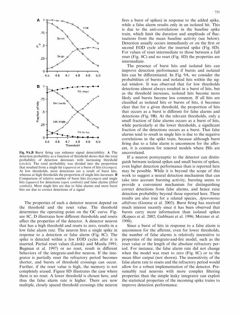
The presence of burst hits and isolated hits canimprove detection performance if bursts and isolatedhits can be differentiated. In Fig. 9A, we consider theprobabilities of bursts and isolated hits within the sig-nal window. It was observed that for low thresholdsdetections almost always resulted in a burst of hits, butas the threshold increases, isolated hits become morelikely and bursts become less common. If all hits areclassified as isolated hits or bursts of hits, it becomesclear that for a given threshold, the proportion of hitsthat occurs as a burst is different for false alarms anddetections (Fig. 9B). At the relevant thresholds, only asmall fraction of false alarms occurs as a burst of hits,while particularly at the lower thresholds, a significantfraction of the detections occurs as a burst. That falsealarms tend to result in single hits is due to the negativecorrelations in the spike train, because although burstfiring due to a false alarm is uncommon for the affer-ent, it is common for renewal models where ISIs areuncorrelated.

If a neuron postsynaptic to the detector can distin-guish between isolated spikes and small bursts of spikes,even higher detection performance than is reported heremay be possible. While it is beyond the scope of thiswork to suggest a neural detection mechanism that cantake into account bursting activity, bursting seems toprovide a convenient mechanism for distinguishingcorrect detections from false alarms, and hence raisedetection probability beyond those reported here. Theseresults are also true for a related species, Apteronotusalbifrons (Goense et al. 2003). Burst firing has receivedmuch interest recently since it has been observed thatbursts carry more information than isolated spikes(Kepecs et al. 2002; Gabbiani et al. 1996; Metzner et al.1998).

Since a burst of hits in response to a false alarm isuncommon for the afferent, even for lower thresholds,the number of false alarms is relatively insensitive toproperties of the integrate-and-fire model, such as thereset value or the length of the absolute refractory per-iod. For instance, the false alarm rate did not changewhen the model was reset to zero (Fig. 8C) or to themean filter output (not shown). The insensitivity of thefalse alarm rate to resets and the refractory period wouldallow for a robust implementation of the detector. Pre-sumably real neurons with more complex filteringproperties than the simple leaky integrator can exploitthe statistical properties of the incoming spike trains toimprove detection performance.

Fig. 9A,B Burst firing can enhance signal detectability. A Thedetection probability as a function of threshold shows that the totalprobability of detection decreases with increasing threshold(circles). The total probability was divided into the proportionthat resulted from a single hit (squares) or a burst of hits (lozenges).At low thresholds, most detections are a result of burst hits,whereas at high thresholds the proportion of single hits increases. BComparison of relative number of burst hits (lozenges) and singlehits (squares) for detections (open symbols) and false alarms (filledsymbols). Most single hits are due to false alarms and most bursthits are due to correct detections of a signal

751

Correlations in the input and output

Since the output of the neural integrator is expected toremain elevated for a time T due to the properties of theintegrator (the correlation time), the response to a falsealarm is also expected to persist for a duration T. Thedetector without reset is thus expected to respond to afalse alarm with a burst of hits. Surprisingly, while this istrue for the models, it is not so for the afferent as weshowed above. This has important implications for sig-nal detection since it suggests that there are mechanismsbuilt into neural activity that can accurately reject falsealarms. This can be seen by comparing the filter outputsfor a false alarm for the afferent and the models. Fig-ure 10 shows a sample trace of the filter output in theneighborhood of a false alarm (top row), and the meanof such traces aligned at the time of the thresholdcrossing (bottom row). For the binomial model (panelA2) the mean filter output did indeed decay with a timeconstant T. But for the afferent, the mean trace (panelD2) decays much faster than the filter time constant.Note also that for the afferent, the peak amplitude of afluctuation is much smaller than that for the models(panels B2–C2).

This faster decay for the afferent is also apparent ifwe examine the auto-covariance function. This is shownin Fig. 11, which shows the auto-covariance function ofthe baseline spike train (top row) and of the filter output(bottom row), for the representative afferent (Fig. 11,

panel D) and the models (panels A–C). The covariancefunction for the binomial spike train (Fig. 11, panel A1)shows that the samples are independent, as expected.The filter output covariance (Fig. 11, A2) has width T(10 EOD cycles), and a correlation time sc of 10.3 EODcycles as predicted from theory. The afferent however,shows an almost identical covariance function for boththe spike train (Fig. 11, panel D1) and filter output(Fig. 11, panel D2). For the afferent the correlation timesc of the filter output is 1.1 EOD cycles. This indicatesthat correlations persist for a very short time, muchshorter than the time constant of the filter. The M0 andM1 models exhibit varying degrees of correlation. ForM0, sc for the filter output is 9.7 EOD cycles, and forM1, which is more regular and shows more narrowing ofthe output covariance function, sc is 5.2 EOD cycles.Median correlation times for the population are 1.41EOD cycles for the afferent (inter-quartile range 1.54),10.5 for B (iqr 0.29), 8.24 for M0 (iqr 2.19), and 4.09 forM1 (iqr 2.70).

Figures 10 and 11 indicate that the filter output isseemingly decorrelated for the afferent. (The Appendixtreats some of the theoretical aspects of the effect of thedecorrelation on sequential detection performance.) Thisdecorrelation has the effect that when there is a falsealarm, the integrator output returns to its baseline valuesvery rapidly, and noise fluctuations are more limited induration. Both the amplitude and duration of the noisefluctuations are smaller for the afferent than for themodels. The smaller amplitude fluctuations are reflectedin the SD (Table 1 and Fig. 4), and have also beenobserved by Ratnam and Nelson (2000) and Chacronet al. (2001). However, in addition to the reduced SD,making use of the property that the noise fluctuations arealso of shorter duration results in an improvement in thedetection performance (Fig. 6) that goes beyond thoseachieved by non-sequential procedures. These properties,of a limited duration and amplitude of the false alarms,suggest that biology may have evolved a strong noisesuppression ability (presumably using anti-correlations).

Fig. 10 Integrator output in the vicinity of a false alarm for therepresentative fiber (D) shown in Fig. 5, and its matched models (Abinomial, B M0, C M1). The spike trains were filtered using a leakyintegrator with time constant T=10. Panels A1–D1: examplesegments of the filter output along with the corresponding stretchof spike train around a false alarm (at t=0). The threshold was setso that Pfa=0.1 for all cases. Fluctuations in the filtered output arelarger for the models. Panels A2–D2: the mean filter output in theneighborhood of a false alarm averaged over all false alarmsegments in the spike train. The panels demonstrate that both theamplitude and the duration of the false alarms for the afferent (D2)are greatly reduced in comparison with the models (A2–C2)

752

Discussion

The methods of detection theory were applied in acontinuous (sequential) framework to P-type electro-sensory afferent spike trains, to study the detectability ofsmall perturbations in the afferent firing rate. We showthat (1) a postsynaptic neuron can function as asequential detector, which integrates the incoming spiketrain and at each instant performs a continuous(sequential) test on the output, to test for the presence ofa signal. An integrate-and-fire neuron can function inthis manner, although other integration schemes, such asthe Hodgkin-Huxley model can also be used; (2) acontinuous detector can detect small increases in firingrate of the input neuron reliably (single spikes), evenwhen the small stimulus-induced changes are superim-posed on a high baseline firing rate; and (3) that thetemporal patterns in the spike train (particularly nega-tive ISI correlations) are central to this ability. Theyimprove detection performance both by decreasing theamplitude of noise fluctuations in the filtered spike train,as well as by limiting the duration of noise fluctuations.We note that negative correlations in spike trains areubiquitous, although it is only recently that they havegenerated greater interest with respect to signal detection(Ratnam and Nelson 2000; Chacron et al. 2001).

Sequential detection

All information about the environment, available to ananimal, is encoded in the form of neural spike trains.The mechanism of encoding information in the spiketrain, and the amount of information contained in spiketrains, both in the firing rate and in the precise timing ofspikes, is well studied (Reich et al. 1997; reviews: Riekeet al. 1997; Borst and Theunissen 1999; Buracas andAlbright 1999). However, how the next higher neurondecodes the signal has received little attention. Since thefirst step is detection of a signal, we applied the methodsof detection theory and sequential analysis to theproblem of detecting a small perturbation in a spiketrain. That this problem is behaviorally relevant hasbeen reported in several studies on detection of smallchanges in spiking activity (Fitzhugh 1957; Bastian 1981;de Ruyter van Steveninck and Bialek 1995; Vallbo 1995;Tougaard 1999; Ratnam et al. 2001; VanRullen andThorpe 2001b).

In weakly electric fish, nearby objects modulate theper-cycle firing probability of P-type afferents. Whenthe object is small or far away the modulations areextremely weak due to the low electrical contrast withthe surrounding water, and so small changes in theafferent firing rate can be obscured by the intrinsicfluctuations in the baseline firing rate. Previous studiesshowed that the behavioral threshold for Apteronotus is<1 lV cm)1 (Knudsen 1974), and in this range theexpected change in firing rate of P-type afferents isabout 1 spike s)1, superimposed on a baseline firingrate of about 300 spikes s)1 (Bastian 1981; Ratnamet al. 2001). Nelson and MacIver (1999) showed thatsmall water fleas (Daphnia magna, 2–3 mm diameter)could be detected at a distance of about 2 cm from thefish. Based on computer reconstructions, they estimatedthat the peak change in the per-cycle probability offiring of an afferent at the time the prey is detected,is about one added spike in a 200-ms window.Ratnam and Nelson (2000) simulated the detectabilityof added spikes using a trial-based approach and

Fig. 11 Auto-covariance functions for the input spike trains (toprow) and filtered output (bottom row), shown for afferent (D) andmatched models (A binomial, BM0, CM1). The afferent is the sameas in Fig. 5. Spike trains were filtered using a leaky integrator withtime constant T=10. The samples of the binomial input spike trainare independent and identically distributed, and so the covariancefunction is zero except at the origin (panel A1), whereas the auto-covariance of the filter output has width T (panel A2). The M0 andM1 models exhibit varying degrees of correlation (panels B1, C1).Note that for M0 the ISIs are independent, but the spike traindemonstrates negative correlations. The output of the integratorshows a more or less narrowing of the covariance function (panelsB2, C2). The afferent, however, shows an almost identicalcovariance function for both input (panel D1) and output (panelD2), i.e., integrating a strongly anti-correlated spike train does notsubstantially increase the correlation time

753

showed that 2–3 extra spikes in a 100-ms window couldbe detected with 90% reliability. While this perfor-mance greatly exceeds those attained by renewal spiketrains (such as Poisson spike trains), it is not adequateto explain the predicted behavioral performance. Thisstudy shows that the trial-based procedure limitsdetection performance, and if a biologically realisticsequential procedure is used, then a detector neuronlocated in the ELL may achieve the predicted perfor-mance (i.e., single spike detection). The single spikesuperimposed on the baseline activity of the electro-sensory afferent can be detected reliably, even thoughthe baseline is highly variable, as judged by the CV ofthe ISI (Kreiman et al. 2000; Ratnam and Nelson2000). The detectability of such small changes agreeswith the observed sensitivity of the electric fish. Weshow that despite the high baseline firing rate, it ispossible to detect a single spike in the afferents in atime that allows for fast behavioral responses(<10 ms). The range of optimal membrane time con-stants found also agrees with the measured time con-stant of the ELL E-cell (Berman and Maler 1998). Afactor that is not taken into account here, but that mayfurther enhance signal detectability is afferent conver-gence. The typical ELL cell receives input from 10–20afferents (Shumway 1989b), and the averaging thisprovides for can enhance detectability if multipleafferents carry a signal. Detecting weak signals is onlyone of the tasks of the ELL. The ELL cells are variablein their morphology and properties (Bastian andNguyenkim 2001) and it has been shown there arethree spatial maps in the ELL (Heiligenberg and Dye1982; Shumway 1989a, 1989b). Furthermore, the spa-tiotemporal tuning of the cells has been shown to de-pend on the type of stimulus (Bastian et al. 2002;Chacron et al. 2003). Thus, how the ELL processes theinformation present in the afferents depends on manyfactors, and although this study shows that it is theo-retically possible to extract one additional spike in asingle afferent using a simple neural mechanism, whe-ther and where in the ELL this happens is still an openquestion.

The implications of this study extend to neural sig-nal detection at large. Detection theory has been ap-plied to neurons since the 1950s (Fitzhugh 1957; Relkinand Pelli 1987; Shofner and Dye 1989; Lee et al. 1993;Celebrini and Newsome 1994). However, the SNR isoften relatively high, i.e., either the baseline activity islow, the changes in response due to the stimulus arehigh, or both. Another drawback of the trial-basedmethod that is typically used is that it does not suggesthow such a scheme may be implemented in a neuron.Furthermore, the long counting periods that are oftenused are not compatible with the speed of neural pro-cessing (Gautrais and Thorpe 1998). Finally, theytypically rely on spike counting, and so most of theinformation contained in the temporal pattern of thespikes is not used. Some methods have expanded onthis by also using temporal information in the spike

train (Geisler et al. 1991; de Ruyter van Steveninck andBialek 1995), and this does improve detection perfor-mance. But we are not aware of a method in which thishas been shown in a biologically realistic setting. In thiswork the detection task was phrased as a sequentialdecision making task. The decision statistic is the out-put of a leaky integrator with the spike train as input.Sequential analysis is sensitive to the temporal pattern(correlation) of the samples. Note also, that in contrastto spike counting, neural integration preserves thetemporal information in the spike train, since the mostrecent spikes are weighted more heavily. This sequen-tial detection scheme can exploit the temporal infor-mation in the spike train, and thereby improvedetection performance. Furthermore, we have shownthat this is readily extended to a biologically realisticneuron, with no loss in performance.

Sequential detection is relevant in many neural sys-tems, since the detection of a small perturbation in aspike train within a short time of its occurrence is ageneral problem in the nervous system. This is impor-tant, since the representation of relevant information,like a sensory signal, by a single spike or very few spikesis common (reviews: Rieke et al. 1997; Parker andNewsome 1998). It has been shown to occur in the visualsystem (Fitzhugh 1957; Barlow et al. 1971; Lee et al.1993; de Ruyter-van Steveninck and Bialek 1995), themechanosensory system (Vallbo 1995), the auditorysystem (Relkin and Pelli 1987; Tougaard 1999), and incortical neurons. The benefit of sequential detection,that decisions are made continuously, becomes impor-tant when quick detection is required, since the timescales of biologically relevant signals and response timesare often short. The response time, or the time to per-ception, has been shown to be on the order of 20–200 ms(de Ruyter van Steveninck and Bialek 1995; Thorpe etal. 1996; Rolls et al. 1999; VanRullen and Thorpe2001a). Sequential detection (continuous signal detec-tion) may be advantageous when the temporal dynamicsof decisions or tracking of the decision statistic isrequired, since it may allow for earlier detection than ispossible using trial-based testing with fixed window size(Kim and Shadlen 1999; Gold and Shadlen 2000;Hernandez et al. 2002).

Role of regularity, correlations and temporalstructure

The sensitivity reported here relies on temporal corre-lations in the spike train, particularly negative correla-tions between adjacent ISIs. Although it has beensuggested that a refractory period introduces negativecorrelations (de Ruyter van Steveninck and Bialek 1995;Berry and Meister 1998; Goldberg 2000; Panzeri andSchultz 2001) and negative correlations, or a high degreeof regularity have been observed in a number of systems(Kuffler et al. 1957; Hagiwara and Morita 1963; Amas-sian et al. 1964; Goldberg and Fernandez 1971; Blanks

754

et al. 1974; Lowen and Teich 1992; Tricas and New1998; Goldberg 2000; Steuer et al. 2001), there is rela-tively little data on their relevance to neural coding. Ithas been shown that negative correlations can improvedetectability of weak signals (Ratnam and Nelson 2000;Chacron et al. 2001), and can increase the informationcontent of the spike train (Stein 1967; Chacron et al.2001; Panzeri and Schultz 2001), but here we establish adirect connection between negative correlations in theISIs and signal detectability.

Correlations can improve detectability in two ways.First, they decrease the SD of the spike count (Ratnamand Nelson 2000; Chacron et al. 2001), or in our case theSD of the neural integrator output (Fig. 4). The smallerSD of the spike count however does not necessarilyrequire negative correlations in the spike train or non-renewality, and thus does not fully explain their possiblefunction; a renewal process can have an equally lowvariability. Here we show that correlations in the spiketrain can improve detectability by a second mechanism,beyond the gain that results from a lower SD. Thenegative correlations result in an effective decorrelationof the filter output, as a result of which random fluctu-ations from the mean also have a shorter duration(Fig. 11), and so a false alarm is less likely. The shortercorrelation time of noise fluctuations makes signalseasier to detect (DeWeese 1996). Furthermore, undercertain conditions, a true detection tends to result inburst firing of the detector neuron, whereas the responseto a false alarm tends to be an isolated spike. Thus,higher-order neurons could use burst firing to furtherimprove detection performance. In weakly electric fish,burst-firing in ELL neurons can increase the informationcarrying capacity (Gabbiani et al. 1996; Metzner et al.1998; Kepecs et al. 2002), and as suggested here, thismay be exploited for improving signal detection per-formance. The short correlation-time of intrinsic fluc-tuations resulting from the anti-correlations in the spiketrain cannot be exploited in a trial-based scheme, butonly in the more biologically plausible scheme ofsequential detection. Thus, the work establishes a con-nection between correlations and sequential detectionperformance, and suggests a biological basis supportingsequential detection.

Behavioral aspects of the detection task

We proposed a biologically plausible method that is ableto exploit correlations in a spike train to achieve highdetection performance. This is a mainly conceptualstudy that highlights important features of the problem,and as such did not address many of the properties thatdetermine whether such a stimulus leads to a perceptionor behavioral response. The detectability of a signal atthe level of the afferent does not necessarily mean it isalso behaviorally relevant. This study shows that a singlespike in the input can in principle be extracted, butwhether this actually happens also depends on many

factors. For instance, the detection performancedepends on the reliability of spike propagation andtransmission, i.e., failures in spike propagation or neu-rotransmitter release. The spatiotemporal properties ofthe neural filters at higher levels in the pathway alsoinfluence detection performance. This is illustrated in thecase of the mechanosensory afferent neuron in thehuman hand, where a single spike was shown to lead to aperception (Vallbo and Johansson 1976; Vallbo 1995).However, whether an afferent spike led to a perceptiondepended on the region of the hand, in some regions onespike sufficed while in others multiple spikes were nee-ded, illustrating the importance of convergence andhigher order spatial filters. We therefore do not presumethat a single spike will always lead to a behavioralresponse and further experiments are needed to addressthis question in the weakly electric fish. Some otherfactors that determine whether such a change in neuralspiking leads to a percept are the acceptable false alarmrate, and which features of the stimulus are important.There is a trade-off between detection probability andfalse alarm rate (Fig. 6), between accuracy and speed(Reddi and Carpenter 2000), sensitivity and resolution(Schiller and Logothetis 1990), and which properties areimportant depends on the neural system, the level, andthe purpose of the system. The relevant false alarm rateis also likely to be different for different neurons andsystems. For example, if low false alarm rates arerequired, it means signals will be missed, but if falsealarms can be eliminated at a later processing stage, suchas by discriminating between burst firing and isolatedspikes, higher false alarm rates may be tolerable. Sensi-tivity can often be increased and false alarms eliminatedby convergence (Shadlen and Newsome 1998), but thisrequires some degree of redundancy, although in sensorysystems, convergence can decrease (spatial) resolution.Besides the detection problem, neurons have to solve anestimation problem. The requirements are not neces-sarily the same for both tasks, and again there may be acompromise. Further studies will be needed to addressthese issues.

Summarizing, physiologists have focused on trial-based testing using aggregate spike counts. This proce-dure is not only biologically unrealistic, but also fails toexploit the mechanisms of dynamic noise-suppression,like the presence of correlations in the spike train. Inbehaving animals the demands of decision making arefar more stringent, and a framework that can exploit thestatistical properties of spike trains, is the continuousdetection method suggested here. The method is realis-tic, and although real neurons have more diverse inte-grative mechanisms, its broad principles and advantagesare likely to remain the same.

Acknowledgements The work was conducted in the laboratory ofDr. Mark E. Nelson (University of Illinois). We would like tothank him for his support, and the comments and suggestions heprovided at various stages of the project. We also thank NouraSharabash and Dr. Zhian Xu for help in collecting data, andDr. Pim van Dijk and Dr. Rob de Ruyter van Steveninck for

755

comments on the manuscript. This work was supported by grantsfrom NIMH (R01-MH49242) and NSF (IBN-0078206) to M.N.The experiments comply with the Principles of animal care, pub-lication No. 86-23, revised 1985, of the National Institute ofHealth and also with the current laws of the United States ofAmerica.

Appendix

Performance comparison between sequentialand trial-based testing

Here we compare the performance of trial-baseddetection and sequential detection with dead-time, anddiscuss the effect of correlations in the spike train onthe performance of the sequential detector. As indi-cated earlier, a direct comparison of the performanceof trial-based testing and sequential testing is notpossible. The decision-making processes are different,since in sequential testing resetting the detector when athreshold is exceeded and restarting the process, trun-cates the PDF under H0 at the threshold value. Con-sequently, calculating d’, r2 and Pfa is not possible insequential testing. This is in contrast to trial-basedtesting where shape of the PDFs under both hypoth-eses is independent of the threshold value. The class ofproblems where testing is stopped and restarted afterthe threshold is reached, or where the integrator isreset, are random walk level-crossing problems. Thetheory underlying these problems has wide applicabil-ity and has received much attention in physics, engi-neering and statistics (Blake and Lindsey 1973;Leadbetter et al. 1983), but closed-form solutions arenot available, even for relatively simple cases such asrenewal spike trains. Given these difficulties, ourinterest is to ask whether there is an equivalent butsimpler process that captures the performance of thesequential scheme, and allows us to calculate the SD ofthe PDF and Pfa. This may allow us to explain theperformance improvement obtained in sequential test-ing and the role of temporal dependencies in the spiketrain on these improvements.

To simplify the sequential testing scheme shown inFig. 3C, we divide y[n] into non-overlapping blocksof length T and examine whether there is at least one hitwithin this block. If the block contains a signal then thehit is a correct detection otherwise it is a false alarm. LetP �d denote the detection probability and P �fa the falsealarm probability for the simplified scheme. To calculatethe probability of detection or false alarm within ablock, we only have to examine the maximum value ofthe T samples within the window. Thus, we can con-struct a sequence yT[k], where k (k‡0) is the number ofblocks of length T as follows:

H0 : yT ½k� ¼ max06i<T

ðy½kT þ i�Þ ðnoise onlyÞ

H1 : yT ½k� ¼ max06i<T

ðy½kT þ i� þ AÞ ðsignalþ noiseÞð3Þ

where i are the individual samples in the block. Signaldetectability will be improved if the SD of the PDFs foryT[k] is smaller than for y[n], since A is the same for bothcases.

Now we can construct the PDFs of yT[k]. It can beshown that if xi is a sequence of independent random

(i.i.d.) variables where 0 £ i<T, the distribution of the

random variable x ¼ max1�i<T

fxig isF ðxÞ ¼QT

i¼1FiðxÞ, where

Fi(x0) is the probability that x<x0 for the ith sample and

F(x0) is the probability that x<x0 for at least one of thesamples within the block. The right tail P(x)=1)F(x).Therefore, if Pfa,i and Pd,i are the probabilities of a falsealarm or detection in a single EOD cycle i within theblock, then the probability of detection P �d is:

P �d ¼ 1�YT

i¼1ð1� Pd;iÞ ð4Þ

The probability of a false alarm is:

P �fa ¼ 1�YT

i¼1ð1� Pfa;iÞ ð5Þ

For a given threshold, it can be shown that theprobabilities (P �d and P �fa) of detecting at least onethreshold crossing in a block, are larger than the prob-abilities of detecting a threshold crossing in one cycle(Pfa,i and Pd,i).

Figure 12A shows the OC for the representativeafferent and its matched binomial model, for thesequential decision method (solid line), and the simpli-fied block-based method (dashed line). For the affer-ent the OC is the same in both cases, whereas forthe binomial model the simplification underestimatesthe performance slightly. For renewal spike trains, thedeviation arises due to the presence of bursts of falsealarms. If a burst of threshold crossings occurs, then inthe sequential scheme, the dead-time is always triggeredon the first threshold crossing. This is not the case forthe block-based scheme and thus bursts are more likelyto spread out over two blocks, and hence the number offalse alarms is somewhat higher. For the afferent, burstsof false alarms only occur when P �d is very close to 1(Fig. 9), but for the models, particularly the binomialmodel, bursts occur more frequently even for small P �dvalues. Hence, for renewal spike trains, the block-basedmethods underestimates P �d for a given P �fa, and is not asgood an approximation of the sequential scheme.

With this simplification we can compare the perfor-mance of the block-based method with the trial-basedmethod. Figure 12B, C shows the ROCs for the repre-sentative afferent and binomial model, where P �d and P �fafollow Eqs. 4 and 5 (solid lines), compared to the trial-based method (dash-dotted line). The figure shows thatfor the afferent there is a large improvement in perfor-mance compared to the trial-based method. For exam-ple, at a Pfa of 0.013, which corresponds to a false alarm

756

rate of 1 Hz, Pd for detecting a spike is 0.83 for theafferent using the sequential scheme while the Pd for thetrial-based scheme is 0.29. For the binomial model thereis hardly any improvement. For this fiber the SD of yT[k]is 0.21 (afferent), 1.04 (B), 0.67 (M0) and 0.34 (M1). Thediscriminability d’ is 3.25 (afferent), 0.63 (B), 1.01 (M0)and 2.03 (M1). The population means of the SD and d’are shown in Table 2.

To examine the role of the correlations in the filteroutput, the filter output was shuffled to remove serialdependencies. Since the filter introduces positive corre-lations in its output, the y[n] are in general not inde-pendent within the time T, and therefore Pd,i and Pfa,i

are not identical and not independent. If, on the otherhand, the y[n] are shuffled so as to remove dependencies,then the samples are independent and identically dis-tributed, and the probabilities Pd,i of detection for eachcycle are equal (Pd), and P �d simplifies to:

P �d ¼ 1� ð1� PdÞT ð6Þ

Similarly for P �fa:

P �fa ¼ 1� ð1� PfaÞT ð7Þ

The ROC for the shuffled afferent filter output (Eqs.6 and 7, Fig. 12B, circles) is almost the same as theROC for the block based afferent output (Eqs. 4 and 5,Fig. 12B, solid line). This suggests the afferent filteroutput samples behave as if they were uncorrelated.The SD of yT[k] for the shuffled output is 0.22 (rep-resentative afferent), the same as without shuffling(0.21). For the models, the SD decreases as a result ofshuffling, as expected. The SD for the shuffled output is0.69 (B), 0.51 (M0), and 0.30 (M1). Table 2 shows thepopulation means. The improvement in the ROC(Fig. 12B) is reflected in the smaller SD of yT[k] com-pared to the SD of y[n]. This follows directly fromEqs. 6 and 7, from which it can be shown that thedistribution of the maximum value of a set of i.i.d.random variables will always have a smaller variancethan the original distribution.

References

Amassian VE, Macy J, Waller HJ, Leader HS, Swift M (1964)Transformations of afferent activity at the cuneate nucleus. In:Gerard RW, Duyff J (eds) Information processing in the ner-vous system. Excerpta Medica Foundation, Amsterdam, pp235–254

Table 2 Discriminability d’ and the SD of the PDF that is obtainedby taking the maximum value attained by the leaky integratoroutput in each block of size T

Filter output Shuffled filter output

d ’ SD of yT[k]

Afferent 3.37±1.06 0.22±0.05 0.22±0.05M1 2.56±1.16 0.32±0.11 0.28±0.09M0 1.65±1.07 0.56±0.24 0.45±0.19B 0.72±0.10 0.94±0.08 0.66±0.04

Shown are the mean±SD of the afferent population (n=49) andtheir matched models. The improved discriminability for theafferents over the models is due to the smaller SD. The right col-umn shows the SD when the filter output is shuffled prior todividing into blocks. For the models shuffling decreases the SD,whereas for the afferent shuffling did not result in a change in theSD, i.e., the filter output for the afferent is apparently decorrelated,as also seen in Fig. 11

Fig. 12A–C Comparison of trial based and sequential detectionschemes. A The sequential scheme (Fig. 3C) is compared to asimplified block based scheme to test the validity of thesimplification. The figure shows the representative afferent inFig. 5 and its matched binomial model (afferent sequential: solidline, afferent block-based overlaps afferent sequential, binomialsequential: dashed line, binomial block-based: dotted line). Thesimplification yields similar performance for the afferent (the curvesare superimposed), but the binomial model shows some differences.The performance of the M0 and M1 models is intermediate (notshown). B ROCs for the simplified scheme (solid line) comparedwith the ROCs obtained from trial-based detection (dash-dot line)for the afferent (dotted line: chance). Sequential detection providesa large performance improvement over trial-based detection. Theopen circles show the performance for the case in which all outputsamples are independent (shuffled filter output), and the perfor-mance is nearly the same as for the afferent, i.e., the filter outputsamples are seemingly decorrelated (Fig. 11). C Results for thebinomial model (as in B). The ROCs are nearly identical for thebinomial model. Thus, sequential detection results in improvedperformance when input spike trains are negatively correlated, butmay not provide much benefit when spike trains are binomial(Poisson)

757

Barlow HB, Levick WR, Yoon M (1971) Responses to singlequanta of light in retinal ganglion cells of the cat. Vision Res[Suppl] 3:87–101

Bastian J (1981) Electrolocation. I. How the electroreceptors ofApteronotus albifrons code for moving objects and other elec-trical stimuli. J Comp Physiol A 144:465–479

Bastian J, Nguyenkim J (2001) Dendritic modulation of burst-likefiring in sensory neurons. J Neurophysiol 85:10–22

Bastian J, Chacron MJ, Maler L (2002) Receptive field organiza-tion determines pyramidal cell stimulus-encoding capability andspatial stimulus selectivity. J Neurosci 22:4577–4590

Berman NJ, Maler L (1998) Inhibition evoked from primaryafferents in the electrosensory lateral line lobe of the weaklyelectric fish (Apteronotus leptorhynchus). J Neurophysiol80:3173–3196

Berry MJ II, Meister M (1998) Refractoriness and neural precision.J Neurosci 18:2200–2211

Blake IF, Lindsey WC (1973) Level-crossing problems for randomprocesses. IEEE Trans Inform Theory 19:295–315

Blanks RHI, Estes MS, Markham CH (1974) Physiologic charac-teristics of vestibular first-order canal neurons in the cat. II.Response to constant angular acceleration. J Neurophysiol38:1250–1268

Borst A, Theunissen FE (1999) Information theory and neuralcoding. Nat Neurosci 2:947–957

Bugmann G, Christodoulou C, Taylor JG (1997) Role of temporalintegration and fluctuation detection in the highly irregularfiring of a leaky integrator neuron model with partial reset.Neural Comput 9:985–1000

Bullock TH, Chichibu S (1965) Further analysis of sensory codingin electroreceptors of electric fish. Proc Natl Acad Sci USA54:422–429

Bullock TH, Heiligenberg W (1986) Electroreception. Wiley, NewYork

Buracas GT, Albright TD (1999) Gauging sensory representationsin the brain. Trends Neurosci 22:303–309

Celebrini S, Newsome WT (1994) Neuronal and psychophysicalsensitivity to motion signals in extrastriate area MST of themacaque monkey. J Neurosci 14:4109–4124

Chacron MJ, Longtin A, St-Hilaire M, Maler L (2000) Supra-threshold stochastic firing dynamics with memory in P-typeelectroreceptors. Phys Rev Lett 21:5328–5343

Chacron MJ, Longtin A, St-Hilaire M, Maler L (2001)Negative interspike interval correlations increase the neuronalcapacity for encoding time dependent stimuli. J Neurosci21:5328–5343

Chacron MJ, Doiron B, Maler L, Bastian J (2003) Non-classicalreceptive field mediates switch in a sensory neuron’s frequencytuning. Nature 423:77–81

Cox DR (1962) Renewal theory. Methuen, LondonDeWeese M (1996) Optimization principles for the neural code.

Network 7:325–331Fitzhugh R (1957) The statistical detection of threshold signals in

the retina. J Gen Physiol 40:925–948Gabbiani F, Koch C (1998) Principles of spike train analysis. In:

Koch C, Segev I (eds) Methods in neuronal modeling: from ionsto networks. MIT, Cambridge, pp 313–360

Gabbiani F, Metzner W, Wessel R, Koch C (1996) From stimulusencoding to feature extraction in weakly electric fish. Nature384:564–567

Gautrais J, Thorpe SJ (1998) Rate coding versus temporal ordercoding: a theoretical approach. Biosystems 48:57–65

Geisler WS, Albrecht DG, Salvi RJ, Saunders SS (1991) Discrim-ination performance of single neurons: rate and temporal-pat-tern information. J Neurophysiol 66:334–362

Goense JBM, Ratnam R, Nelson ME (2003) Burst firing improvesthe detection of weak signals in spike trains. Neurocomput 52–54:103–108

Gold JI, Shadlen MN (2000) Representation of a perceptual deci-sion in developing oculomotor commands. Nature 404:390–394

Gold JI, Shadlen MN (2001) Neural computations that underliedecisions about sensory stimuli. Trends Cogn Sci 5:10–16

Goldberg JM (2000) Afferent diversity and the organization ofcentral vestibular pathways. Exp Brain Res 130:277–297

Goldberg JM, Fernandez C (1971) Physiology of peripheralneurons innervating semicircular canals of the squirrel monkey.III. Variations among units in their discharge properties.J Neurophysiol 34:676–684

Green D, Swets J (1966) Signal detection theory and psychophys-ics. Wiley, New York.

Hagiwara S, Morita H (1963) Coding mechanisms of electrore-ceptor fibers in some electric fish. J Neurophysiol 28:784–799

Heiligenberg W, Dye J (1982) Labeling of electroreceptive afferentsin a gymnotic fish by intracellular injection of HRP: the mysteryof multiple maps. J Comp Physiol 148:287–296

Hernandez A, Zainos A, Romo R (2002) Temporal evolution of adecision-making process in medial premotor cortex. Neuron33:959–972

Kashimori Y, Goto M, Kambara T (1996) Model of P- andT-electroreceptors of weakly electric fish. Biophys J 70:2513–2526

Kepecs A, Wang X-J, Lisman J (2002) Bursting neurons signalinput slope. J Neurosci 22:9053–9062

Kim J-N, Shadlen MN (1999) Neural correlates of a decision in thedorsolateral prefrontal cortex of the macaque. Nat Neurosci2:176–185

Knudsen EI (1974) Behavioral thresholds to electric signals in highfrequency electric fish. J Comp Physiol 91:333–353

Kreiman G, Krahe R, Metzner W, Koch C, Gabbiani F (2000)Robustness and variability of neuronal coding by amplitudesensitive afferents in the weakly electric fish Eigenmania.J Neurophysiol 84:189–204

Kuffler SW, Fitzhugh R, Barlow HB (1957) Maintained activity inthe cat’s retina in light and darkness. J Gen Physiol 40:683–702

Lansky P, Musila M (1991) Variable initial depolarization inStein’s neuronal model with synaptic reversal potentials.Biol Cybern 64:285–291

Leadbetter MR, Lindgren G, Rootzen (1983) Extremes and relatedproperties of random sequences and processes. Springer, BerlinHeidelberg New York

Lee BB, Wehrhahn C, Westheimer G, Kremers J (1993)Macaque ganglion cell responses to stimuli that elicit hypera-cuity in man: detection of small displacements. J Neurosci12:1001–1009

Lowen SB, Teich MC (1992) Auditory-nerve action potentials forma nonrenewal point process over short as well as long timescales. J Acoust Soc Am 92:803–806

Metzner W, Koch C, Wessel R, Gabbiani F (1998) Featureextraction by burst-like spike patterns in multiple sensory maps.J Neurosci 18:2283–2300

Nelson ME, MacIver MA (1999) Prey capture in the weakly elec-tric fish Apteronotus albifrons: sensory acquisition strategies andelectrosensory consequences. J Exp Biol 202:1195–1203

Nelson ME, Xu Z, Payne JR (1997) Characterization and modelingof P-type electrosensory afferent responses to amplitudemodulations in a wave-type electric fish. J Comp Physiol A181:532–544

Panzeri S, Schultz SR (2001) A unified approach to the study oftemporal, correlational and rate coding. Neural Comput13:1311–1349

Parker AJ, Newsome WT (1998) Sense and the single neuron:probing the physiology of perception. Annu Rev Neurosci21:227–277

Ratnam R, Nelson ME (2000) Non-renewal statistics of electro-sensory afferent spike trains: implications for the detection ofweak sensory signals. J Neurosci 20:6672–6683

Ratnam R, Goense JBM, Nelson ME (2001) The response ofP-type electrosensory afferents to weak prey-like stimuli. 6th IntCongr Neuroethol, Bonn

Reddi BA, Carpenter RH (2000) The influence of urgency ondecision time. Nat Neurosci 3:827–30

Reich DS, Victor JD, Knight BW, Ozaki T, Kaplan E (1997)Response variability and timing precision of neuronal spiketrains in vivo. J Neurophysiol 77:2836–2841

758

Relkin EM, Pelli DG (1987) Probe tone thresholds in the auditorynerve measured by two-interval forced-choice procedures.J Acoust Soc Am 82:1679–1691

Rieke F, Warland D, Ruyter van Steveninck RR de, Bialek W(1997) Spikes: exploring the neural code. MIT Press, Cambridge

Rolls ET, Tovee MJ, Panzeri S (1999) The neurophysiology ofbackward visual masking: information analysis. J Cogn Neu-rosci 11:300–311

Rossum M van (2001) A novel spike distance. Neural Comput13:751–763

Ruyter van Steveninck R de, Bialek W (1995) Reliability and sta-tistical efficiency of a blowfly movement-sensitive neuron. Phi-los Trans R Soc Lond B 348:321–340

Ruyter van Steveninck R de, Lewen GD, Strong SP, Koberle R,Bialek W (1997) Reproducibility and variability in neural spiketrains. Science 275:1805–1808

Schiller PH, Logothetis NK (1990) The color-opponent and broad-band channels of the primate visual system. Trends Neurosci13:392–398

Shadlen M, Newsome WT (1998) The variable discharge of corticalneurons: implications for connectivity, computation, andinformation coding. J Neurosci 18:3870–3896

Shofner WP, Dye RH (1989) Statistical and receiver operatingcharacteristic analysis of empirical spike count distributions:quantifying the ability of cochlear nucleus units to signalintensity changes. J Acoust Soc Am 86:2172–2184

Shumway CA (1989a) Multiple electrosensory maps in the medullaof weakly electric gymnotiform fish. I. Physiological differences.J Neurosci 9:4388–4399

Shumway CA (1989b) Multiple electrosensory maps in the medullaof weakly electric gymnotiform fish. II. Anatomical differences.J Neurosci 9:4400–4414

Siegmund D (1985) Sequential analysis: test and confidence inter-vals. Springer, Berlin Heidelberg New York

Stein RB (1967) The information capacity of nerve cells using afrequency code. Biophys J 7:797–826

Steuer R, Ebeling W, Russell DF, Bahar S, Neiman A, Moss F(2001) Entropy and local uncertainty of data from sensoryneurons. Phys Rev E 64:061911, 1–6

Thorpe SJ, Fize D, Marlot C (1996) Speed of processing in thehuman visual system. Nature 381:520–522

Tougaard J (1999) Receiver operating characteristics and temporalintegration in an insect auditory receptor cell. J Acoust Soc Am106:3711–3718

Tricas TC, New JG (1998) Sensitivity and response dynamics ofelasmobranch electrosensory primary afferent neurons to nearthreshold fields. J Comp Physiol A 182:89–101

Vallbo AB (1995) Single-afferent neurons and somatic sensation inhumans. In: Gazzaniga MS (ed) The cognitive neurosciences.MIT Press, Cambridge, pp 237–252

Vallbo AB, Johansson (1976) Skin mechanoreceptors in the humanhand: neural and psychophysical thresholds. In: Zotterman Y(ed) Sensory functions of the skin. Pergamon Press, Oxford, pp185–199

VanRullen R, Thorpe SJ (2001a) The time course of visual pro-cessing: from early perception to decision-making. J CognNeurosci 13:454–461

VanRullen R, Thorpe SJ (2001b) Rate coding versus temporalorder coding: what the retinal ganglion cells tell the visualcortex. Neural Comput 13:1255–1283

Wald A (1947) Sequential analysis. Wiley, New YorkXu Z, Payne JR, Nelson ME (1996) Logarithmic time course of

sensory adaptation in electrosensory afferent nerve fibers in aweakly electric fish. J Neurophysiol 76:2020–2032

759