Analytical Procedures for Continuous Data Level Auditing: Continuity

Equations 1

Alexander Kogan Michael G. Alles

Miklos A. Vasarhelyi

Department of Accounting & Information SystemsRutgers Business School

Rutgers University180 University AveNewark, NJ 07102

Jia WuDepartment of Accounting and Finance

University of Massachusetts – Dartmouth285 Old Westport Road

North Dartmouth, MA 02747

July 4, 2010

1 Comments are welcome and may be addressed to Miklos A. Vasarhelyi at miklosv@rutgers.edu. We thank the KPMG CA/R/Lab at Rutgers Business School for support. We also thank participants, and especially the discussant, Tony Tinker, at the Four Schools Conference at Baruch College for helpful feedback, as well as Carol Brown and participants at the 2005 and 2006 American Accounting Association Meetings. We thank the participants of multiple AAA, AICPA, and IIA conferences for their comments on this paper. All views expressed in this paper are those of the authors alone.

Analytical Procedures for Continuous Data Level Auditing: Continuity Equations

Abstract:

This paper designs a Continuous Data Level Auditing system utilizing business process based analytical procedures and evaluates the system’s performance using disaggregated transaction records of a large healthcare management firm. An important innovation in the proposed architecture of the CDA system is the utilization of analytical monitoring as the second (rather than the first) stage of data analysis. The first component of the system utilizes automatic transaction verification to filter out exceptions, defined as transactions violating formal business process rules. The second component of the system utilizes business process based analytical procedures, denoted here “Continuity Equations”, as the expectation models for creating business process audit benchmarks. Our first objective is to examine several expectation models that can serve as the continuity equation benchmarks: a Linear Regression Model, a Simultaneous Equation Model, two Vector Autoregressive models, and a GARCH model. The second objective is to examine the impact of the choice of the level of data aggregation on anomaly detection performance. The third objective is to design a set of online learning and error correction protocols for automatic model inference and updating. Using a seeded error simulation approach, we demonstrate that the use of disaggregated business process data allows the detection of anomalies that slip through the analytical procedures applied to more aggregated data. Furthermore, the results indicate that under most circumstances the use of real time error correction results in superior performance, thus showing the benefit of continuous auditing.

Keywords: continuous auditing, analytical procedures, error correction.Data availability: The data is proprietary. Please contact the authors for details.119Equation Chapter 9 Section 1

1

I. IntroductionContinuous Auditing with Transaction Data Availability

Business is in the process of a fundamental transformation towards the digital economy (Vasarhelyi and Greenstein 2003). With many companies having implemented networked integrated Enterprise Resource Planning (ERP) systems (such as SAP ERP, Oracle E-Business Suite, PeopleSoft Enterprise) as part of the core of their basic information infrastructure, management and control of organizations is shifting to a data-centric, process-oriented paradigm.2 The requirements of Section 404 of the Sarbanes-Oxley Act for rigorous controls over financial reporting also focus attention on how data is processed and used within the company, while the mining of customer and operational data is essential for company’s pursuing strategies of customer satisfaction and total quality control.

In response to these fundamental changes in the business environment, public accounting firms and internal auditing departments are now facing the opportunities and challenges associated with the development and deployment of continuous auditing (CA) which comprises largely automated data intensive audit procedures with decreased latency between the transaction event and the provision of assurance.3 In the limit, the auditor would access real time streams of the entire universe of the company’s transactions rather than being restricted to a small sample gathered at a single moment of time (as in the annual inventory count). The feasibility of creating such a real time, automated audit methodology arises from

2 Vasarhelyi and Greenstein (2003).3 The CICA/AICPA report defines CA as “a methodology that enables independent auditors to provide written assurance on a subject matter using a series of auditors’ reports issued simultaneously with, or a short period of time after, the occurrence of events underlying the subject matter.” http://www.cica.ca/index.cfm/ci_id/989/la_id/1.htm

2

the capability of the company’s systems to make available to auditors business data of far finer granularity in time and detail than has ever been cost effectively accessible before.4

Continuous auditing is becoming an increasingly important area in accounting, both in practice and in research, with conferences held around the world attended by both academics and practitioners.5 The major public accounting firms all have CA initiatives under way, and major software vendors are also now aggressively developing and marketing CA software solutions. PricewaterhouseCoopers (2006) in their survey state that “Eighty-one percent of 392 companies responding to questions about continuous auditing reported that they either had a continuous auditing or monitoring process in place or were planning to develop one. From 2005 to 2006, the percentage of survey respondents saying they have some form of continuous auditing or monitoring process within their internal audit functions increased from 35% to 50%—a significant gain.”6 On the research front, the ongoing survey of the CA research literature by Brown et al. (2006) lists at least 60 papers in the area, ranging from behavioral research to system design, analytical models and implementation case studies.

Notably, however, there is a dearth of empirical research or case studies of new CA methodological developments due to the lack of data availability and difficulties of access to companies implementing CA. As a consequence, what is missing from both the academic and professional literatures is a rigorous examination of the new CA methodology, and in particular, how auditing will cope with the shift from data scarcity to data wealth, from periodic and archival to real time streaming data. This is a critical omission since much of

4 Vasarhelyi et al. (2004). 5 Alles et al. (2006b).6 CFO.com, June 26, 2006.

3

existing audit practice, methods and standards are driven by lack of data and the cost of accessing it: hence auditors do sampling, establish materiality thresholds for investigations and carry out analytical procedures before substantive testing of details so that they can focus only on likely trouble spots. Will any of these familiar practices survive in an age of digital economy with substantially reduced costs and increased capabilities of data storage, access and communication?

While a cost/benefit analysis supports an auditor choosing to base audit procedures on limited data when data is very costly to obtain, it is harder to defend continuing to constrain the analysis when transaction level raw (unfiltered) business data is readily available. It is the latter situation that the audit profession will increasingly face until auditing procedures and systems are developed that can exploit the availability of timely and highly disaggregated data. In other words, the audit profession has to either answer the question of what it plans to do with all the data that it is progressively obtaining, data which provides the level of detail an order of magnitude beyond the sampled, highly aggregated data that is the basis of much of the current audit methodology—or else, to explain why data is being thrown away unused. It is incumbent on the auditors to develop methodologies that exploit that opportunity so that they can provide their clients with higher quality, more effective and efficient audits.

One of the hypotheses driving this research is that making use of the transaction level data one can design expectation models for analytical procedures which have an unprecedented degree of correspondence to underlying business processes. Creating business process based benchmarks requires data at a highly disaggregated level, far below the level of account balances that are used in most

4

analytical procedures today, such as ratio or trend analysis. Testing the content of a firm’s data flow against such benchmarks focuses on examining both exceptional transactions and exceptional outcomes of expected transactions. Ideally, CA software will continuously and automatically monitor company transactions, comparing their generic characteristics to observed/expected benchmarks, thus identifying anomalous situations. When significant discrepancies occur, alarms will be triggered and routed to the appropriate stakeholders.

The objective of this project is to explore the benefits of using business process based analytical procedures to create a system of continuous data level auditing.

An important innovation in the proposed architecture of the CA system is the utilization of analytical monitoring as the second (rather than the first) stage of data analysis. The first component of the proposed CA system utilizes automatic transaction verification to filter out exceptions, which are transactions violating formal BP rules. The second component of the system creates business process audit benchmarks, which we denote as Continuity Equations (CE), as the expectation models for process based analytical procedures. The objective of having audit benchmarks consisting of CEs is to capture the dynamics of the fundamental business processes of a firm, but since those processes are probabilistic in nature, the CEs have to be data driven statistical estimates. Once identified, CEs are applied to the transaction stream to detect statistical anomalies possibly indicating business process problems.

We validate the proposed CA system design using a large set of the supply chain procurement cycle data provided by a large healthcare management firm. This allows us to examine what form the CEs will take in a real world setting and how effective they are in detecting errors. While the data is not analyzed in real time, the

5

extent of the data we use mimics what a working data level CA system would have to deal with and it provides a unique testing ground to examine how audit procedures will adapt to deal with the availability of disaggregated data. In order to maintain the integrity of the database and to avoid slowing down priority operational access to it, the data will be fed in batches to the CA system. But even daily downloads undertaken overnight will still provide a far reduced latency between transaction and assurance than anything available today.

Transaction detail data are generated by three key business processes in the procurement cycle: the ordering process, the receiving process, and the voucher payment process. The CE models of these three processes are estimated using the statistical methodologies of linear regression, simultaneous equation modeling, and vector autoregressive models. We design a set of online learning and error correction protocols for automatic model inference and updating. We use a seeded error simulation study to compare the anomaly detection capability of the discussed models. We find that under most circumstances the use of real time error correction results in superior performance. We also find that each type of CE models has its strengths and weaknesses in terms of anomaly detection. These models can be used concurrently in a CA system to complement one another. Finally, we demonstrate that the use of disaggregated data in CE can lead to better anomaly detection when the seeded errors are concentrated, while yielding no improvement when the seeded errors are dispersed.

In summary, the results presented in this paper show the effectiveness benefits of continuous data level auditing over standard audit procedures. Firstly, the use of disaggregated business process data allows the detection of anomalies that slip through the analytical procedures applied to more aggregated data. In particular, our results

6

show that certain seeded errors, which are detected using daily, are not detected using weekly metrics. There is even less chance to detect such errors using monthly or quarterly metrics, which is the current audit practice. Secondly, the enabling of real time error correction protocol provides effectiveness benefits above and beyond the use of disaggregated business process data. Even if conventional audit takes advantage of such data, it will not achieve the same level of anomaly detection capability as continuous data level audit since, as shown by the results in this paper, certain anomalies will not be detected without prior correction of previous anomalies. Since conventional auditors will have to investigate all the anomalies at the end of the audit period, the time pressure of the audit is likely to prevent from rerunning their analytical procedures and conducting repeated additional investigations to detect additional anomalies after some previously detected ones are corrected.

The remainder of this paper is organized as follows. Section 2 provides a review of the relevant literature in auditing, CA, business processes and AP upon which our work is based and to which the results of the paper contribute. Section 3 describes the design and implementation of data-oriented CA systems, Section 4 discusses the critical decision choice of how to aggregate the transactional data, and the CE model construction using three different statistical methods, with Section 5 comparing the ability of the CE-based AP tests in detecting anomalies under various settings. Section 6 discusses the results, identifies the limitations of the study, and suggests future research directions in this domain. Section 7 offers concluding comments.

7

II. Literature ReviewThis paper draws from and contributes to multiple streams of

literature in system design, continuous auditing and analytical procedures.

Continuous AuditingThe initial papers on continuous auditing are Groomer and

Murthy (1989) and Vasarhelyi and Halper (1991). They pioneered the two modern approaches toward designing the architecture of a CA system: the embedded audit modules and the control and monitoring layer, respectively. The literature on CA since then has increased considerably, ranging from the technical aspects of CA (Kogan et al. 1999, Woodroof and Searcy 2001, Rezaee et al. 2002, Murthy 2004, Murthy and Groomer 2004, etc.) to the examinations of the economic drivers of CA and their potential impact on audit practice (Alles et al. 2002 and 2004, Elliott 2002; Vasarhelyi 2002, Searcy et al. 2004). Kogan et al. (1999) propose a program of research in CA. In the discussion of the CA system architecture they identify a tradeoff in CA between auditing the enterprise system versus auditing enterprise data. A study by Alles et al. (2006) develops the architecture of a CA system for the environment of highly automated and integrated enterprise system processes, and shows that a CA system for such environments can be successfully implemented on the basis of continuous monitoring of business process control settings. A study published by the Australian Institute of Chartered Accountants (Vasarhelyi et al, 2010) summarizes the extant state of research and practice in CA.

This paper focuses on the enterprise environment in which many business processes are not automated and their integration is lacking, and proposes to design a CA system architecture based on data-oriented procedures. In this development, it utilizes the approach

8

of Vasarhelyi et al. (2004) that introduces four levels of CA assurance having different objectives. More specifically, this paper develops a CA methodology for the first and third CA levels: transaction verification and assurance of higher-level measurements and aggregates.7

The unavailability of data to researchers is the likely cause of a lack of empirical and case studies on CA in general and on analytical procedures for CA in particular. This paper contributes to the CA literature by providing empirical evidence to illustrate the advantages of CA in real-time problem resolution. More specifically, we show that potential problems can be detected in a more timely fashion, at the transaction stream level as opposed to the account balance level. Traditionally, analytical procedures are applied at the account balance level after the business transactions have been aggregated into account balances. This would not only delay the detection of potential problems but also create an additional layer of difficulty for problem resolution due to a large number of transactions that are aggregated into accounting numbers. The focus on auditing the underlying business processes alleviates this problem by utilizing much more disaggregated information in continuous auditing.

We develop a CA data-oriented methodology around the key economic processes of the firm. This approach can also be viewed as an extension to CA of the modern business process auditing approach proposed by Bell et al. (1997). They advocate a holistic approach to auditing an enterprise: structurally dividing a business organization into various business processes (e.g. the revenue cycle, procurement cycle, payroll cycle, and etc.) for the auditing purpose. They suggest the expansion of the focus of auditing from business transactions to the routine activities associated with different business processes.

7 The other two levels are compliance and judgment verification.

9

Vasarhelyi and Halper (1991) are the first to take advantage of online technology and modern networking to develop a procedure for continuous auditing. Their study introduces the concept of continuous analytical monitoring of business processes, and discusses the use of key operational metrics and analytics to help internal auditors monitor and control AT&T’s billing system. They use the operational process auditing approach and emphasize the use of metrics and analytics in continuous auditing. This is the first study to adopt the term “Continuity Equations” which is used in modeling of how billing data flowed through business processes and accounting systems at AT&T. The choice of the expression by Vasarhelyi and Halper is driven by the fact that as with the conservation laws in physics, in a properly functioning accounting control system there should not be any “leakages” from the transaction flow.

This paper develops the application of the concept of CE to model the relationships between the metrics of key business processes, while building on the original implementation of CA as described in Vasarhelyi and Halper (1991). The broader implications of their model have been obscured in the subsequent focus of the CA literature on technology enablers and the frequency of reporting. Attaining the full potential of CA requires the utilization of not only of its well known capability of decreasing audit latency, but also of taking advantage of data availability to create audit benchmarks that are not only timelier but provide more accurate, detailed and dynamic models of fundamental business processes.

Analytical ProceduresAuditing is defined as “a systematic process of objectively

obtaining and evaluating evidence regarding assertions about economic actions and events to ascertain the degree of correspondence between those assertions and established criteria and

10

communicating the results to interested users.”8 Thus the scope of auditing is driven not only by what evidence is available, but also whether there exist benchmarks—the “established criteria”—to compare that audit evidence against. Those benchmarks provide guidance about what the data is supposed to look like when drawn from a firm operating without any anomalies.

One of the key roles played by benchmarks in modern auditing is in the implementation of Analytical Procedures (AP), which Statement on Auditing Standards (SAS) No. 56 defines as the “evaluation of financial information made by a study of plausible relationships among both financial and nonfinancial data”. SAS 56 requires that analytical procedures be performed during the planning and review stages of an audit, and recommends their use in substantive testing in order to minimize the subsequent testing of details to areas of detected concern. That sequence is dictated because manually undertaken tests of detail are so costly that they are resorted to only if the account balance based AP tests indicate that there might be a problem. Both the timing and nature of standard analytical procedures are thus brought into question in a largely automated continuous auditing system with disaggregated data. Analytical procedures reduce the audit workload and cut the audit cost because they help auditors focus substantive tests of detail on material discrepancies.

There are extensive research studies on analytical procedures in auditing. Many papers discuss various analytical procedures ranging from financial ratio analysis to linear regression modeling that focus on highly aggregated data such as account balances (Hylas and Ashton 1982, Kinney 1987, Loebbecke and Steinbart 1987, Biggs et al. 1988, Wright and Ashton 1989, Hirst and Koonce 1996). The percentages of errors found using such analytical procedures are 8 Auditing Concepts Committee (1972, page 18).

11

usually not high, varying between 15% and 50%. Only a few papers examine analytical procedures for more disaggregated data. Dzeng (1994) compares 8 univariate and multivariate AP models using quarterly and monthly financial and non-financial data of a university, and concludes that disaggregated data yields better precisions in a multivariate time-series based expectation model. Other studies also find that applying AP models to higher frequency monthly data can improve analytical procedure effectiveness (Chen and Leitch 1998 and 1999, Leitch and Chen 2003, Hoitash et al. 2006). By contrast, Allen et al. (1999) use both financial and non-financial monthly data of a multi-location firm and do not find any supporting evidence that geographically disaggregate data can improve analytical procedures.

In this study we build a data level CA system which utilizes CE based analytical procedures applied to even more highly disaggregate daily metrics of business processes. We investigate several different probabilistic models of those business processes to serve as our CE based audit benchmark: the Linear Regression Model (LRM), the Simultaneous Equation Model (SEM), the Vector Autoregressive Models (VAR), and the Generalized Autoregressive Conditional Heteroscedasticity (GARCH) model. The use of SEM in analytical procedures has been examined by Leitch and Chen (2003), but only using monthly financial statement data. Their finding indicates that SEM can generally outperform other AP models including Martingale and ARIMA.

As far as we can ascertain, the Vector Autoregressive Model has not been fully explored in the auditing literature. There are a number of studies utilizing univariate time series models (Knechel 1988, Lorek et al. 1992, Chen and Leitch 1998, Leitch and Chen 2003), but only one, by Dzeng (1994), which uses VAR. Dzeng concludes that VAR is better than other modeling techniques in generating expectation

12

models, and he specifically recommends using Bayesian VAR (BVAR) models. The computational complexity of VAR used to hamper its application as an AP model, since appropriate statistical tools were not readily available in the past. However, the recent developments in statistical software facilitate the application of this sophisticated model.9 The VAR model can not only represent the interrelationships between BPs but also capture their time series properties. Although (to the best of our knowledge) VAR has been discussed only once in the auditing literature, studies in other disciplines have either employed or discussed VAR as a forecasting method (see e.g., Swanson 1998, Pandher 2002). Detailed statistical development of the VAR methodology and related issues can be found in Enders (2004).

The GARCH model is a time series model that uses past variances to forecast current period variances (Enders 2003 and Engle 2001). Since it can capture the volatility of time series data, it is widely used in financial economics literature (Lamoureux and Lastrapes 1990; Hentschel 1995, Heston and Nandi 2000). This study includes the GARCH model as a CE candidate to check whether the utilization of past variance information can improve the identification of BP anomalies.

III. Design and Implementation of a Continuous Data Level Auditing System

The objective of a CA system designed in this study is to provide close to real-time assurance on the integrity of certain enterprise business processes. As in conventional auditing, such a system can utilize two different types of procedures: those monitoring business process controls and those substantively analyzing business process transactions. As Alles et al. (2006) indicate, business process control

9 Starting with version 8, SAS (Statistical Analysis System) allows users to make multivariate time series forecasts using an advanced VARMAX procedure.

13

monitoring requires that the client possesses a modern integrated IT infrastructure, and faces challenges even then. They also show that even today few firms have the type of tight, end to end system integration that continuous control monitoring depends upon. This paper focuses on designing a CA system for the much more common enterprise environments in which data is derived from multiple legacy systems that lack centralized and automated controls. This lack of a control based monitoring system is why the proposed CA system is data-oriented instead, and the provision of assurance is based on verifying transactions and on business process based analytical procedures. Where the IT environment allows, CA would ideally encompass both continuous (data level) assurance (CDA) and continuous control monitoring (CCM)10.

The architecture of the designed data level CA system is driven by the procedures it has to implement. While the subject matter it deals with is quite different from that in conventional auditing, one can view its procedures as analogous to automated substantive audit procedures, including detailed transaction testing and analytical procedures. Therefore, the two main components of the CA system are those executing automatic transaction verification and CE based automatic analytical business process monitoring, as shown in Figure 1.

[Insert Figure 1 here]

A salient feature of the architecture we propose in Figure 1 is the Business Data Warehouse which serves as the data integration point for the disparate (mostly legacy) systems in the enterprise system landscape. As explained below, in a large enterprise environment, the lack of such data warehouse would make a CA

10 See Alles et al. (2006b) and Alles et al. (2007) for the discussion of continuous control monitoring.

14

system infeasible due to the prohibitive complexity, cost and complications associated with data access.

An important innovation in the proposed architecture of the CA system presented in Figure 1 is the utilization of analytical monitoring as the second (rather than the first) stage of data analysis. In conventional (manual) auditing, testing transactional details is very laborious and has to be based on statistical sampling to control the cost of auditing. Therefore, analytical procedures are utilized first for the identification of areas of concern to focus the sampling on. In CA, which utilizes automated transaction verification tests, there is no need for sampling, since automated tests can be easily applied to the complete population of business transactions.

The implementation of the transaction verification component of the CA system is based on identifying business process rules and formalizing them as transaction integrity and validity constraints. Every recorded transaction is then checked against all the formal rules in the component, and if it violates any of the rules, then the transaction is flagged as an exception. Every exception generates a CA alarm in the CA system, which it sends to the appropriate parties for resolution. Since the alarm specifies which formal business process rules are violated by the exception, resolving exceptions should be a fairly straightforward task. Once the transaction data is verified, it is in an acceptable form to be used to develop the CE based audit benchmarks for AP.

Detailed Data ProvisioningEnterprise systems that support key business processes

routinely collect business process data in the unfiltered highly disaggregated form. If the enterprise has implemented an integrated ERP system, then BP data is readily available in the ERP central database. However, the most common current situation is that the

15

enterprise system landscape consists of a patchwork of different systems, many of which are legacy ones and are often file-based. In such enterprise systems direct real-time access to business process data is highly problematic, if at all possible at any reasonable expense of time and effort. Therefore, a data-oriented CA system usually cannot be cost-effectively deployed in such environment unless the enterprise deploys an overlay data repository commonly known as “Business Data Warehouse”. This is a relational database management system specially designed to host business process data provided by the other enterprise systems, including the legacy cycle-focused ones (such as sales processing or accounts receivable). While the main functionality of a data warehouse is online analytical processing, the CA system developed here relies only on its function as the global repository of business process data. The availability of disaggregated business process data makes it possible for the auditor to access any raw, unfiltered and disaggregated data that is required for the construction and operation of CE based AP tests, and is thus the critical enabler of the proposed CA system.

Data Description Our simulated implementation of the data-oriented CA system

focuses on the procurement-related business processes and utilizes the data sets extracted from the data warehouse of a healthcare management firm with multi-billions of dollars in assets and close to two hundred thousand employees. The firm is a major national provider of healthcare services, with a network composed of locally managed facilities that include numerous hospitals and outpatient surgery centers all over the US and overseas. A key strategic driver for the firm is the management of their supply chain which provides everything from paper towels to heart/lung machines to their various

16

operating units through dozens of warehouses spread throughout the United States.

The organization provided extracts from their transactional data warehouse which, while only a sample limited in time and geography, still encompassed megabytes of data, several orders of magnitude more detailed than anything typically examined in a standard audit. The data sets include all procurement cycle daily transactions from October 1st, 2003 through June 30th, 2004. The number of transaction records for each activity ranges from approximately 330,000 to 550,000. These transactions are performed by ten facilities of the firm including one regional warehouse and nine hospitals and surgical centers. The data was first collected by the ten facilities and then transferred to the central data warehouse in the firm’s headquarters.

Transaction VerificationFollowing the BP auditing approach, as the first step, we

identify the following three key business processes in the supply chain procurement cycle: ordering, receiving, and voucher payment, which involve six tables in our data sets. Since this data is uploaded to the data warehouse from the underlying legacy system, there are numerous data integrity issues, which have to be identified by the transaction verification component of the CA system before the data is suitable for AP testing. To simulate the functionality of the transaction verification component, we formally specify various data validity, consistency, and referential integrity constraints, and then filter through them all the available transactions.

Two categories of erroneous records are removed from our data sets: those that violate data integrity and those that violate referential integrity.

17

Data integrity violations include but are not limited to invalid purchase quantities, receiving quantities, and check numbers.11

Referential integrity violations are largely caused by many unmatched records among different business processes. For example, a receiving transaction cannot be matched with any related ordering transaction. A payment was made for a non-existent purchase order.

Before any analytical model can be built, these erroneous records must be eliminated. This removal simulates the action of the transaction verification component of the CA system. Potentially, in a very tightly integrated enterprise environment with automated business process controls, such transactional problems may have been prevented by the client’s ERP system.

An additional step in the transaction filtering phase is to delete non-business-day records. Though we find that sporadic transactions have occurred on some weekends and holidays, the number of these transactions accounts for only a small fraction of that on a working day. However, if we leave these non-business-day records in the sample, these records would inevitably trigger false alarms simply because of low transaction volume.

While the simulated verification of transactions relied on fairly straightforward business rules described above, the client firm considered that just the exceptions identified at this stage were a major source of value added from the project. It is to be anticipated that as legacy systems are gradually superseded by the firm’s ERP system with stronger automated controls, the transaction verification component of the CA system will be catching fewer and fewer

11 We found negative or zero numbers in these values which can not always be justified by our data provider.

18

problems. Conversely, the fact that any were caught at all indicates the value of this element of automated continuous auditing, since these transaction level errors had escaped detection by the standard practices being employed by the firm’s internal auditors.

Business Process Based Analytical ProceduresThe transaction verification stage of continuous data level

auditing is based on user specified rules designed to catch obvious errors in individual business events. The object of analytical procedures is the “study of plausible relationships among both financial and nonfinancial data” in order to detect anomalous patterns in the firm’s performance and the way in which it is reported.

The implementation of the analytical procedure (AP) component of the CA system first requires creation of the process level continuity equations which can provide benchmarks for these tests. Instead of testing transaction by transaction for obvious errors, the AP test contrasts the stream of data against a probabilistic model of what that data should look like if there were no untoward events happening in the firm. Such models usually take the form of statistically stable relationships between business process metrics (and possibly some exogenous factors). Every business process metric is calculated over a subset of transactions corresponding to intervals along some important business process dimensions (such as time, region, product, customer, etc). Since the relationship between the metrics holds only probabilistically, the model also has to specify the acceptable range of variation of the residuals. An anomaly arises when the observed values of the metrics result in residuals which fall outside this acceptable range. Every anomaly generates a CA alarm in the CA system, which it sends to the appropriate parties for resolution. A

19

rating of the seriousness of the error could also be passed along to these parties.

In contrast with an exception, which is associated to an individual transaction, an anomaly is associated with a subset of transactions used to calculate the values of the metrics. Therefore, the resolution of an anomaly is not straightforward. Moreover, an anomaly is not necessarily indicative of a problem, since it can be due to statistical fluctuation.

As mentioned above, in the workflow of the proposed data-oriented CA system the first stage of processing is the verification of transactions. It has to be contrasted with the fact that in conventional auditing analytical procedures are used first to identify areas of concern, and then transaction testing is focused on the identified risky areas. The rationale for this sequence is that it makes it possible to reallocate the sample counts so as to increase either the effectiveness or the efficiency of substantive testing. Since in this CA system the verification of transactions is automatically performed, it can be applied to the entire population of data without the need for sampling. Therefore, the transaction verification component of the CA system processes every transaction in the business process stream, and serves as a filter screening out the identified exceptions. Then this filtered stream of transactions is further processed by the analytical procedures component of the system to ascertain the absence of anomalies. Thus, the CA system reverses the sequence of procedures of traditional auditing to capitalize on the capabilities of modern IT to verify the entire stream of business transactions against the formalized set of process rules.

The rationale for analytical procedures in the proposed CA architecture is many-fold. First, one can never assume that the set of formalized business process rules completely defines the set of

20

constraints business transactions have to satisfy. Given this possibility, analytical procedures serve as the second line of defense. Anomalies identified by the CA system can signal the presence of likely abnormal transactions that are not discovered by the user defined rules of the transaction verification filter. This is an indication either of some exceptional event, such as fraud, or if the anomaly occurs often enough, of the need to update the rule set of the transaction verification system. Additionally, analytical procedures can be a critical “second line of defense” if the transaction verification component fails for whatever reason.

Second, analytical procedures can identify certain business process irregularities that cannot be caught in principle by the transaction verification component because they are not due to the violation of any business rules. For example, in this specific area of procurement, there is a possibility that a batch of purchase orders may be destroyed without any notification by the delivery mechanism external to the enterprise. In this case, the unexpected drop-off in item deliveries can be identified as anomalous by the analytical procedures, which will thus provide the precious early warning of a process problem. Another procurement-related example has to do with regular payments of vendor invoices to take advantage of early payment discounts. Then, the process rules may not require payments before the invoice due date, while the practice is to pay early. If, say, due to a staffing change in the accounts payable department, the early payments are not processed on time, there will be no violation of process rules, but the analytical procedures would still be able to signal an anomaly after identifying an unexpected decline in the number of payments processed. Human investigations of anomalies identified by the analytical procedures should be able to discern the root cause of the anomalies (if any) and initiate the necessary

21

corrective actions. It may be possible to introduce additional artificial intelligence / expert systems techniques to differentiate “real” anomalies from those due to statistical fluctuation (see e.g., Murthy and Swanson 1992).

Another reason that necessitates the use of analytical procedures in CA is due to the possibility that individual transactions may be in perfect compliance with the business process rules and all pass the transaction verification stage, while taken together they deviate from the desirable behavior. Such instances include the so-called “channel stuffing” or the breaking-up of purchase orders to circumvent the authorization limit.

At this stage of this research project into continuous data level assurance we are only investigating the efficacy of CE based AP tests in detecting generic errors. Much more research is needed to create a library of anomalous business patterns that can be loaded into the CA system and serve to direct human auditors to particular problem areas. Before that can happen, we must first show that it is possible to create process level benchmarks, the continuity equations, in the first place.

IV Models of Continuity EquationsFollowing the BP auditing approach, the three key business

processes for the obtained sample were ordering, receiving, and voucher payment processes. The analytical procedures component of the CA system is based on benchmarks which model the interrelationships between these processes. A critical issue in modeling business processes analytically is the choice of BP metrics. The traditional accounting choice has been the use of financial measures (e.g., dollar amounts), driven in the first place by the reliance on ledger entries as the primary source of data. In a data environment where disaggregate data is available, however, modeling

22

business processes can also be undertaken using other types of non-financial metrics such as physical measurements or document counts. The dollar amounts of each transaction or the number of transactions processed can also be used. In this study the transaction item quantity is selected as the BP metric. There is no conceptual reason why analytical procedures cannot utilize multiple metrics to examine transaction flows. 12 Auditing on different metrics would enable auditors to detect a more diverse set of patterns of firm behavior.13

Once the BP metrics are chosen, the next step is to determine the appropriate degree of aggregation at which it is appropriate to conduct the AP test, and hence, the characteristics of the data used to construct the CE based benchmark.

Data AggregationThe main argument against using aggregated data is that it

inevitably leads to a loss of information about individual transactions. Thus, investigating an anomalous aggregated business process metric requires an examination of a large number of transactions that were aggregated to calculate the metric. But aggregation can also make it possible to see more general patterns. There has been extensive debate in the profession over how and to what extent to aggregate transactional data, and whether to use ledger accounts as a means of summarizing data. The key difference is that in a disaggregated data environment and with the technical ability to process such large data

12 The advanced audit decision support systems used at AT&T (Vasarhelyi and Halper 1991) provided views of different variables if chosen by the auditor including: number of calls, minutes, dollars and modified dollars).13 We need to perform audits on different metrics besides financial numbers. For example, the Patriot Act requires that banks should report the source of money for any deposit larger than US$100,000 by its client. However, the mandatory reporting controls can be bypassed by dividing the deposit over $100,000 into several smaller deposits. Even though the deposit amount each time is under the limit, the total number of deposits should be a cause for concern. Auditors can only catch such fraudulent activity by using the number of deposit transactions as one of the audit metrics.

23

sets, the degree and nature of aggregation is now a choice that is open to auditors to make, rather than one forced on them by measurement constraints.

The main statistical argument for aggregation is that it can reduce the variability observed among individual transactions. For example, the transaction quantity can differ greatly among individual transactions, as well as the lag time between order and delivery, and delivery and payment. By aggregating the individual transactions, this variance can be significantly reduced, thus allowing more effective detection of material anomalies. The fluctuations among individual transactions can also be smoothed by aggregation, which facilitates the construction of a stable model. Otherwise, it would be infeasible to derive a stable model based on data sets with large variances because the model would either trigger too many alarms or lack the detection power. On the other hand, if individual transactions are aggregated over a longer time period such as a week or a month, then the model would fail to detect many abnormal transactions because the abnormality would be mostly smoothed out by the longer time interval. Thus, the inescapable tradeoff that the more aggregated the metrics are, the more stable the analytical relationships are likely to be at a price of more missed detection. In the mean time, any anomaly involving a metric with higher level of aggregation, requires a more extensive (and expensive) investigation of the larger subpopulation of transactions if an alarm is triggered. Daily and weekly aggregations used in this analysis are natural units of time that should result in a reasonable trade-off between these two forces. Aggregation can be performed on other dimensions besides the time interval, and the choice of the aggregation levels has to be made on a case by case basis considering the inherent characteristics of the underlying transactional data.

24

This study uses intermediate aggregates of transactions, such as aggregates of transactions of different units in the enterprise, aggregates of transactions with certain groups of customers or vendors. This is a novelty since traditional substantive testing is done either at the most disaggregated level, or at the most aggregated level. Substantive tests of details of transactions are done at the most disaggregated level of individual transactional data, but this is done in order to verify the correctness of that individual transaction rather than to gain a perspective of the overall business process. Tests of details of account balances are obviously applied at the most aggregated level. All standard analytical procedures are used for analyzing the account balances or the largest classes of transactions. As our results show, analysis of intermediate aggregates can provide more confidence when making audit judgments about anomalies and give the auditor a means of thinking about the underlying business process as a whole.

Summary statistics of the data used in the analysis are presented in Table 1.

[Insert Table 1 here]

As discussed above, we select transaction item quantity as the primary metric for testing as opposed to dollar amounts, and we do so for two reasons: First, we want to illustrate that CA can work efficiently and effectively on operational (non-financial) data; second, in our sample set dollar amounts contain noisy information including sales discounts and tax. We aggregate the transaction quantities for the ordering, receiving, and voucher payment processes respectively. After excluding weekends and holidays and several observations at the beginning of the sample period to reduce noises in the sample, we have 180 days of observations in our data sets for each business process.

25

Continuity Equations: Simultaneous Equation ModelWe investigate probabilistic models that can serve as candidates

for our continuity equation benchmarks of the firm’s supply chain processes: a Simultaneous Equation Model (SEM), Vector Autoregressive (VAR) models, a Linear Regression Model (LRM) and a GARCH model. The SEM can model the interrelationships between different business processes simultaneously while the linear regression model can only model one relationship at a time, but the latter is less computationally demanding. In SEM each interrelationship between two business processes is represented by an equation and the SEM-based CE model consists of a simultaneous system of two or more equations which represent the business processes that make up the organization.

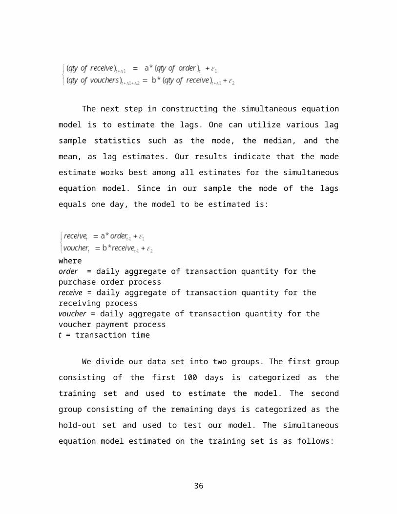
In SEM and LRM we specify the daily aggregate of order quantity as the exogenous variable while the daily aggregates of receiving quantity and payment quantity are endogenous variables. Time stamps are added to the transaction flow among the three business processes. The transaction flow originates from the ordering process at time t. After a lag period Δ1, the transaction flow appears in the receiving process at time t+ Δ1. After another lag period Δ2, the transaction flow re-appears in the voucher payment processes at time t+Δ2. Taking into account the possibility of partial or combined deliveries, as well as partial or combined payments, the application of the SEM methodology to these procurement processes yields the following set of equations:14

14 Alles et al. (2006b) develop these statistical CE relationships from the underlying theoretical business processes of the firm’s supply chain. In this paper adopt a purely statistical approach towards CE creation.

26

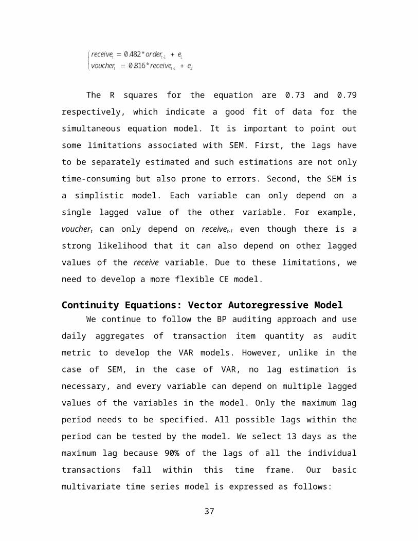
The next step in constructing the simultaneous equation model is to estimate the lags. One can utilize various lag sample statistics such as the mode, the median, and the mean, as lag estimates. Our results indicate that the mode estimate works best among all estimates for the simultaneous equation model. Since in our sample the mode of the lags equals one day, the model to be estimated is:

whereorder = daily aggregate of transaction quantity for the purchase order processreceive = daily aggregate of transaction quantity for the receiving processvoucher = daily aggregate of transaction quantity for the voucher payment processt = transaction time

We divide our data set into two groups. The first group consisting of the first 100 days is categorized as the training set and used to estimate the model. The second group consisting of the remaining days is categorized as the hold-out set and used to test our model. The simultaneous equation model estimated on the training set is as follows:

The R squares for the equation are 0.73 and 0.79 respectively, which indicate a good fit of data for the simultaneous equation model. It is important to point out some limitations associated with SEM. First, the lags have to be separately estimated and such estimations are not only time-consuming but also prone to errors. Second, the SEM is a simplistic model. Each variable can only depend on a single

27

lagged value of the other variable. For example, vouchert can only depend on receivet-1 even though there is a strong likelihood that it can also depend on other lagged values of the receive variable. Due to these limitations, we need to develop a more flexible CE model.

Continuity Equations: Vector Autoregressive ModelWe continue to follow the BP auditing approach and use daily

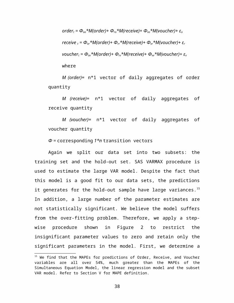
aggregates of transaction item quantity as audit metric to develop the VAR models. However, unlike in the case of SEM, in the case of VAR, no lag estimation is necessary, and every variable can depend on multiple lagged values of the variables in the model. Only the maximum lag period needs to be specified. All possible lags within the period can be tested by the model. We select 13 days as the maximum lag because 90% of the lags of all the individual transactions fall within this time frame. Our basic multivariate time series model is expressed as follows:

ordert = Φoo*M(order)+ Φro*M(receive)+ Φvo*M(voucher)+ εo

receive t = Φor*M(order)+ Φrr*M(receive)+ Φvr*M(voucher)+ εr

vouchert = Φov*M(order)+ Φrv*M(receive)+ Φvv*M(voucher)+ εv

where

M (order)= n*1 vector of daily aggregates of order quantity

M (receive)= n*1 vector of daily aggregates of receive quantity

M (voucher)= n*1 vector of daily aggregates of voucher quantity

28

Φ = corresponding 1*n transition vectors

Again we split our data set into two subsets: the training set and the hold-out set. SAS VARMAX procedure is used to estimate the large VAR model. Despite the fact that this model is a good fit to our data sets, the predictions it generates for the hold-out sample have large variances.15 In addition, a large number of the parameter estimates are not statistically significant. We believe the model suffers from the over-fitting problem. Therefore, we apply a step-wise procedure shown in Figure 2 to restrict the insignificant parameter values to zero and retain only the significant parameters in the model. First, we determine a p-value threshold for all the parameter estimates.16 Then, in each step, we only retain the parameter estimates under the pre-determined threshold and restrict those over the threshold to zero, and re-estimate the model. If new insignificant parameters appear, we restrict them to zero and re-estimate the model. We repeat the step-wise procedure several times until all the parameter estimates are below the threshold, resulting in a Subset VAR model.

[Insert Figure 2 here]

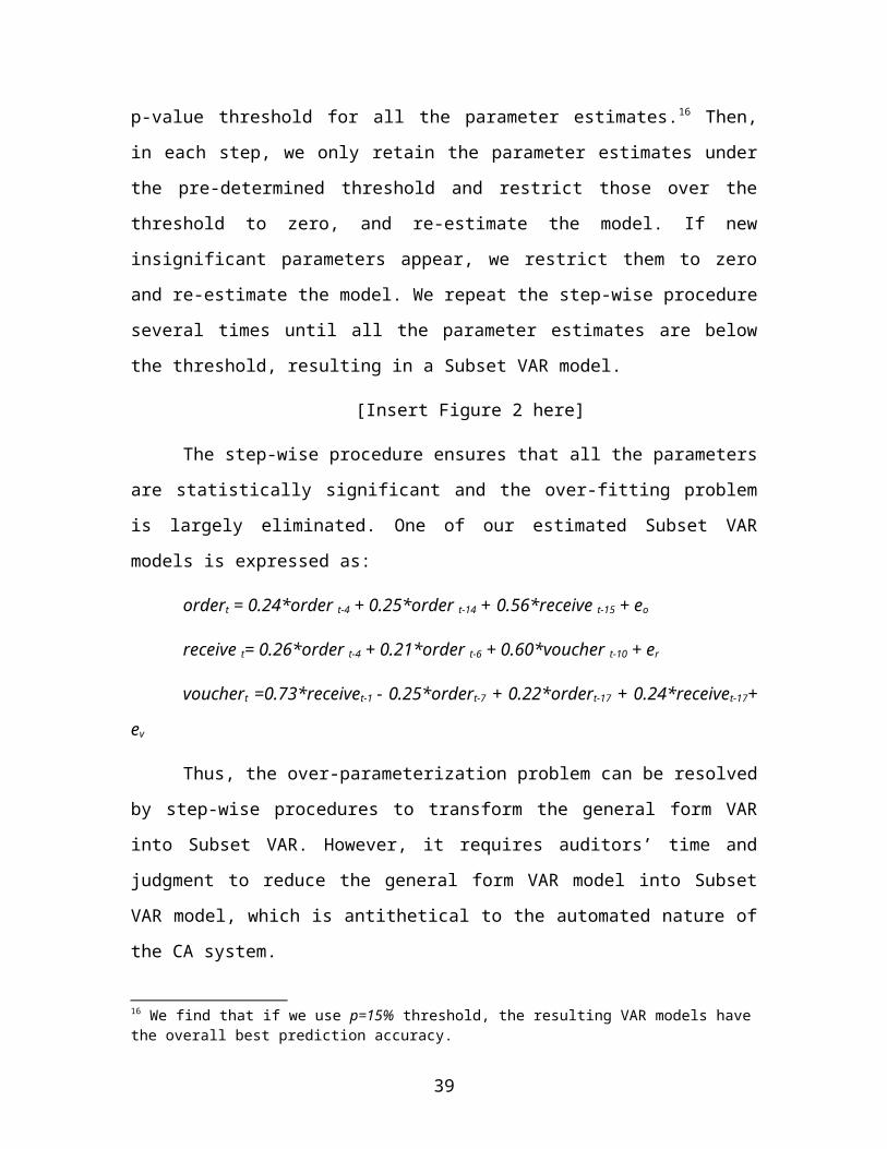
The step-wise procedure ensures that all the parameters are statistically significant and the over-fitting problem is largely eliminated. One of our estimated Subset VAR models is expressed as:

ordert = 0.24*order t-4 + 0.25*order t-14 + 0.56*receive t-15

+ eo

receive t= 0.26*order t-4 + 0.21*order t-6 + 0.60*voucher t-10 + er

15 We find that the MAPEs for predictions of Order, Receive, and Voucher variables are all over 54%, much greater than the MAPEs of the Simultaneous Equation Model, the linear regression model and the subset VAR model. Refer to Section V for MAPE definition.16 We find that if we use p=15% threshold, the resulting VAR models have the overall best prediction accuracy.

29

vouchert =0.73*receivet-1 - 0.25*ordert-7 + 0.22*ordert-17 + 0.24*receivet-17+ ev

Thus, the over-parameterization problem can be resolved by step-wise procedures to transform the general form VAR into Subset VAR. However, it requires auditors’ time and judgment to reduce the general form VAR model into Subset VAR model, which is antithetical to the automated nature of the CA system.

Recent development in Bayesian statistics, however, allows the model itself to control parameter restrictions. The BVAR model includes prior probability distribution functions to impose restrictions on the parameter estimates, with the covariance of the prior distributions controlled by “hyper-parameters”. In other words, the values of hyper-parameters in the BVAR model control how far the model coefficients can deviate from their prior means and how much the model can approach an unrestricted VAR model (Doan et al. 1984, Felix and Nunes 2003). The BVAR model can release auditors from the burden of parameters restriction to derive the Subset VAR model. Thus, in this study we utilize both the BVAR and Subset VAR variants of the VAR model.

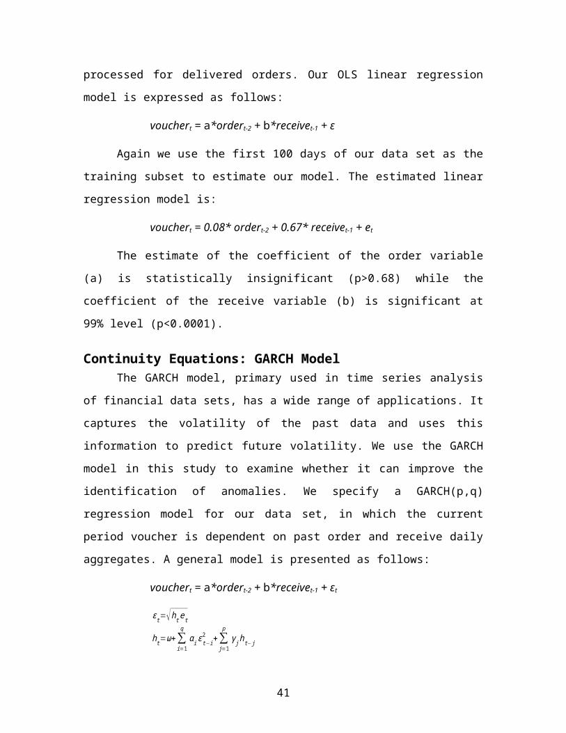
Continuity Equations: Linear Regression ModelIn the linear regression model we specify the lagged values of

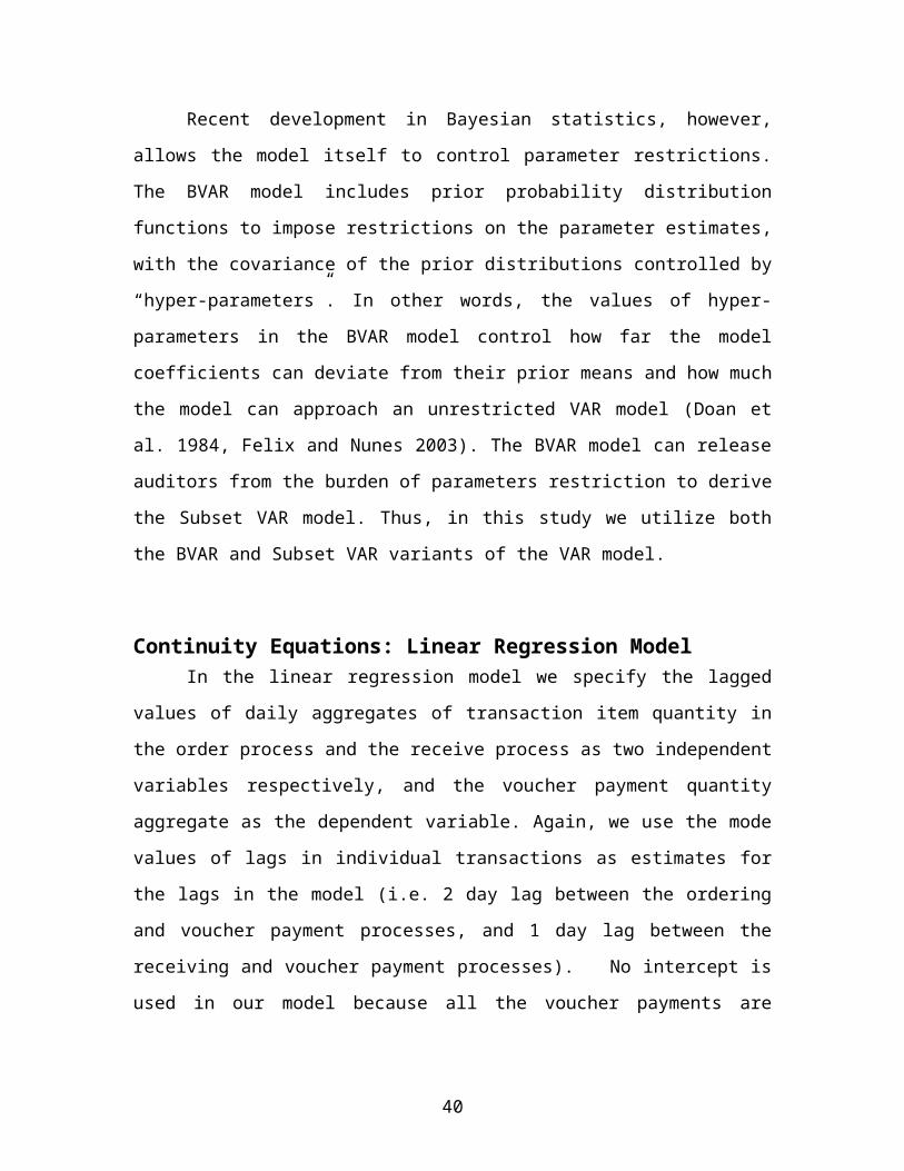
daily aggregates of transaction item quantity in the order process and the receive process as two independent variables respectively, and the voucher payment quantity aggregate as the dependent variable. Again, we use the mode values of lags in individual transactions as estimates for the lags in the model (i.e. 2 day lag between the ordering and voucher payment processes, and 1 day lag between the receiving and voucher payment processes). No intercept is used in our model because all the voucher payments are processed for

30

delivered orders. Our OLS linear regression model is expressed as follows:

vouchert = a*ordert-2 + b*receivet-1 + ε

Again we use the first 100 days of our data set as the training subset to estimate our model. The estimated linear regression model is:

vouchert = 0.08* ordert-2 + 0.67* receivet-1 + et

The estimate of the coefficient of the order variable (a) is statistically insignificant (p>0.68) while the coefficient of the receive variable (b) is significant at 99% level (p<0.0001).

Continuity Equations: GARCH ModelThe GARCH model, primary used in time series analysis of

financial data sets, has a wide range of applications. It captures the volatility of the past data and uses this information to predict future volatility. We use the GARCH model in this study to examine whether it can improve the identification of anomalies. We specify a GARCH(p,q) regression model for our data set, in which the current period voucher is dependent on past order and receive daily aggregates. A general model is presented as follows:

vouchert = a*ordert-2 + b*receivet-1 + εt

ε t=√ht etht=ω+∑

i=1

q

αi ε t−i2 +∑

j=1

p

γ jh t− j

where e t~ IN(0,1), ω > 0, αi > 0, γj > 0

εt = the residual used for GARCH estimation

Due to the limitations of the current SAS version (9.1), we have to use the AUTOREG procedure with GARCH parameters (instead of VARMAX GARCH) for the anomaly detection purpose. This approach

31

basically modifies our estimation of the the linear regression model to account for possible heteroscedasticity. We utilize the most common variant GARCH(1,1) of the model. An example of the regression part of the estimated model is shown as follows:

vouchert=0 .0788∗order t−2+0 . 6645∗receivet−1+εt

Online Model Learning ProtocolOne distinctive feature of analytical modeling in CA is the

automatic model selection and updating capability. Traditional analytical modeling is usually based on static archival data sets. Auditors generally apply one model to the entire audit dataset. In comparison, analytical modeling in CA can be based on the continuous data streams dynamically flowing into the CA system. The analytical modeling in CA thus has the potential to assimilate the new information contained in every segment of the data flows and adapt itself constantly. The online model learning protocol we utilize in this study is shown in Figure 3. Each newly updated analytical model is used to generate a prediction only for one new segment of data. In the first step shown in Figure 3, data segments from 1 through 100 are used to estimate the model and use it to predict the new segment 101. After that, the new segment (101) is used together with the previous dataset to infer the next model. If the size of the previous dataset is small, the new segment is simply added without removing the oldest one from the dataset, as shown in Figure 3. After the dataset used for model inference becomes sufficiently large, it is preferable to use the so-called “sliding window” approach, in which the size of the training dataset is kept constant, and the addition of a new data segment is combined with removing the oldest one. This model updating procedure is expected to improve prediction accuracy and anomaly detection capability.

32

[Insert Figure 3 here]

V. Anomaly Detection Comparison across CE ModelsMAPE Comparison

While performing analytical procedures, auditors use various methods to make predictions on account numbers. It is desirable for expectation models to make forecasts as close to actual values as possible. Many prior AP studies evaluate expectation models in terms of prediction accuracy (Kinney 1978, Wild 1987, Dzeng 1994, Allen et al. 1999, Chen and Leitch 1998, Leitch and Chen 2003). Following this line of research, we compared the prediction accuracies for the CE models in this study using a measure of prediction accuracy called Mean Absolute Percentage Error (MAPE). Additionally, we compared the CE models on their error detection ability.

MAPE, the absolute value of the difference between the predicted value and the actual value measured as a percentage of the actual value, is a commonly used metric of prediction accuracy. It is expected that a good model should have a small MAPE. The training set is first used to estimate each of the models. Then, each estimated model is used to make one-step-ahead forecasts and the forecast variance is calculated. After that, the model is updated based on the new data feeds in the hold-out set and the previous steps are repeated. Finally, all the absolute variances are summed up and divided by the total number of observations in the hold-out sample to compute the MAPE. The results for MAPE of Voucher predictions are presented in Table 2.

[Insert Table 2 here]The results indicate that as measured by the MAPE metric the

prediction accuracies of these models are close. The BVAR version of the VAR model has the best prediction accuracy (MAPE=0.3330),

33

followed by the Subset VAR model (MAPE=0.3374), though the standard deviation for the BVAR model is slightly higher than that of the Subset VAR. The SEM has the lowest prediction accuracy of 0.3499. These prediction accuracies indicate that the forecasts generated by the expectation models usually differ from the reported amounts by approximately 30%.

There are no universal criteria to determine whether these prediction accuracies are good or not because MAPE values are data dependent. Prior studies (Kinney 1978, Wild 1987, Chen and Leitch 1998) on expectation models indicate that large variances exist in prediction accuracies when different data sets are used. The MAPE values reported in Wild’s (1987) study range from 0.012 for Cost of Goods Sold prediction to 7.6 for Cash and Security prediction using the same expectation model. Our conclusion is that by the MAPE metric, all candidate CE models show promise as benchmarks for AP tests.

Error Detection Ability Comparison A continuity equation is a means towards an end and not an end

in itself. The rationale for constructing a CE-based AP test is to enable the detection of anomalies effectively and efficiently. Thus while predicting the value of a variable with low MAPE is desirable, more useful is the ability to detect errors.

To measure the detection capability of the three CE models we use two metrics: the number of false positive errors and the number of false negative errors.17 A false positive error, also called a false alarm or a type I error, is a non-anomaly mistakenly detected by the model as an anomaly. A false negative error, also called a type II error, is an anomaly not detected by the model. While a false positive error can waste auditor’s time and thereby increase audit cost, a false 17 For the presentation purposes, we also include the tables and charts showing the detection rate, which equals 1 minus the false negative error rate.

34

negative error is usually more detrimental because of the material uncertainty associated with the undetected anomaly. An effective and efficient AP model should keep both the number of false positive errors and the number of false negative errors at a low level.

To compare the anomaly detection capabilities of the CE models under different settings we randomly seed eight errors into the hold-out sample. We also test how the error magnitude can affect each AP model’s anomaly detection capability with five different magnitudes used in every round of error seeding: 10%, 50%, 100%, 200% and 400% of the original value of the seeded observations. The entire error seeding procedure is repeated ten times to reduce selection bias and ensure randomness.18

Prior AP studies discuss several investigation rules to identify an anomaly (Stringer 1975, Kinney and Salaman 1982, Kinney 1987). A modified version of the statistical rule (Kinney 1987) is used in this study. Prediction intervals (PI), equivalent to a confidence interval for an individual dependent variable, are used as the acceptable thresholds of variance. If the value of the prediction exceeds either the upper or lower limits of the PI, then the observation is flagged as an anomaly.

The selection of the prediction interval is a critical issue impacting the effectiveness of the AP test. The size of the prediction interval is determined by the value of the significance level α. Choosing a low α value (e.g. 0.01), leads to wide tolerance boundaries (i.e. large prediction interval) and a resulting low detection rate. On the other hand, if a high α value is selected, then the prediction

18 Leitch and Chen (2003) use both positive and negative approaches to evaluate the anomaly detection capability of various models. In the positive approach all the observations are treated as non-anomalies. The model is used to detect the seeded errors. In contrast, the negative approach treats all observations as anomalies. The model is used to find the non-anomalies. This study only adopts the positive approach because it fits better the established audit practice for AP tests.

35

interval will be overly narrow and many normal observations will be flagged as anomalies. To solve this problem, we have followed two approaches to select the prediction interval percentages. In the first approach, α values are selected to control the number of false positive errors in various models. More specifically, an α value is selected which is just large enough to yield two false positive errors in the training data set. In the second approach, which is the traditional one, predetermined α values, 0.05 and 0.1, are used for all the expectation models.

Before we can use this methodology to compare the CE models, another critical issue needs to be addressed, an issue that only arises in a continuous audit setting: real time error correction.

Real-time Error CorrectionAn important distinction between CA techniques and standard

auditing that was explored in this project is what we call “Real Time Error Correction”. In a CA environment when an anomaly is detected, the auditor will be notified immediately and a detailed investigation, if relevant, can be initiated. In theory, the auditor can then have the ability to correct the error before the next round of audit starts.

Whether this technical possibility can or will be carried out in practice depends both upon the speed at which error correction can be made and the more serious issue of the potential threat to auditor independence of using data in subsequent tests that the auditor has had a role in correcting. These issues clearly require detailed consideration, but what we focused on at this stage was quantifying the benefits of real time error correction in a CA environment. These issues clearly require detailed consideration, but doing so is beyond the scope of the current study. What we focus on here is the technical implication for AP in CA if errors are indeed detected and corrected in real time in a CA environment. Specifically, when the AP model

36

detects a seeded error in the hold-out sample, we examine the consequences on subsequent error detection if the seeded error is corrected by substitution of the original value before the model is used again.

For comparison purpose, we test how our candidate CE models work with and without real time error correction. Unlike continuous auditing, anomalies are detected but usually not corrected immediately in traditional auditing. To simulate this scenario, we don’t correct any errors we seeded in the hold-out sample even if the AP model detects them.

[Insert Table 3 here]One can argue that it is possible in principle to utilize error

correction in traditional auditing. However, since traditional auditors will have to investigate all the anomalies at the end of the audit period, the time pressure of the audit is likely to prevent them from rerunning their analytical procedures and conducting additional investigations over and over again to detect additional anomalies after some previously detected errors are corrected.

Overall, the results show lower false negative error rates for all CE models with error correction, especially when the error magnitude is large (100% or more). This finding is consistent with the prior expectation. Under some rare circumstances, the non-correction model has slightly better detection rate than the correction model. All these exceptions occur when the error magnitude is small (no larger than 50 percent). Higher false positive error rates, mostly when error magnitudes are large, are observed for the error-correction models, which means that the error-correction models can detect more anomalies but at a cost of triggering more false alarms. However, a further investigation reveals that the false alarms are mostly caused by certain records in the holdout sample, which are called in this

37

study “original anomalies”. These original anomalies are very likely to be caused by measurement errors since our dataset consists of un-audited operational data. This measurement error problem with non-audited data is also reported by previous studies (Kinney and Salamon 1982, Wheeler and Pany 1990). Because the non-correction model would not correct those undetected errors, the impact of original anomalies, whose values remain constant, would be eclipsed by the increase in seeded error magnitude. Therefore, the non-correction model would trigger fewer false alarms when the magnitude in seeded error increases. On the other hand, the impact of original anomalies would not decrease as the error-correction model would correct all detected errors.

Auditors are usually more averse to false negative errors than to false positive errors if the false positive error rate is kept at a reasonable level. The cost of false positive errors is only a waste of auditor’s time and effort, while the cost of false negative errors can be potentially catastrophic and detrimental to the client firm and auditor’s reputation. In summary, the error-correction models have better anomaly detection performance than the non-correction models. Thus, the real time error correction protocol can improve the anomaly detection performance, and the enabling of this protocol is an important benefit of continuous auditing.

Another noteworthy finding is that the α value, as expected, controls the tradeoff between the false positive and false negative error rates. A large α value leads to more false positive errors but fewer false negative errors. Meanwhile, a small α value leads to fewer false positive errors but more false negative errors. It should also be noted that even though the BVAR model generally has the best detection performance, its false positive rate is also the highest among all models. Another finding is that even though we use the α value which only yields two false positive errors in the training data

38

set for each CE model, the number of false positive errors generated in the hold-out sample is not equal among the CE models. This study does not control the number of false positive errors in the hold-out sample because it can lead to a look-ahead problem. Specifically, the data in the hold-out sample can not be used to construct CE models since they would not be available in the real world when the auditor builds expectation models.

Disaggregated versus Aggregated DataThis study examines if the use of disaggregated data can make

CE models perform better than based on the aggregated data. Data can be aggregated on different dimensions, and we compare the efficacy of CE based AP tests using temporal and geographic disaggregation.

In the temporal disaggregation analysis we examine the differential anomaly detection performances using weekly versus daily data. Errors are seeded into the weekly data in the same fashion as in previous simulations. We follow prior studies (Kinney and Salamon 1982, Wheeler and Pany 1990) in the choice of methods to seed errors into the daily data. In the best case scenario, the entire weekly error is seeded into a randomly selected day of a week. In the worst case scenario, the weekly error is first divided by the number of working days in a week (five) and then seeded into each working day of that week. In addition to the different aggregation levels of data comparison, the error-correction and non-correction models are again compared to verify if the previous findings still hold. Due to the scope of this study we only use a single α value 0.05 in all models. The results are presented in Figure 4 A/B for the BVAR model.

[Insert Table 4 and Figure 4 in here]The results are generally consistent with our expectations. In

terms of detection ability, all the CE models perform the best using

39

the best case scenario daily data, followed by the weekly data. All the models have the poorest anomaly detection performance using the worst case scenario daily data. This result is not surprising because the weekly error is spread evenly into each day making the seeded error act as a systematic error which is almost impossible to detect (Kinney 1978). With respect to false positive error rates, the results are mixed. We believe that the original anomalies in our data sets caused this problem. In the cross model comparison the BVAR model generally detects more errors than other models but at the same time triggers more false alarms. The linear regression model generally has fewer false alarms but suffers from low detection rate when error magnitudes are small.

We repeat the analyses aggregating data on the geographic dimension and obtain similar results. Overall, our results show that the use of disaggregated business process data allows the detection of anomalies that slip through the analytical procedures applied to more aggregated data (normally utilized in traditional auditing), thus demonstrating the effectiveness of CA.

VI DiscussionLimitations of the Analysis

Our data sets are extracted from a single firm, which may constitute a selection bias. Until we test our data level CA system using other firms’ data sets, we will not have empirical evidence to support the claim that our AP models are portable and can be applied to other firms. In addition, our data sets contain noise, as indicated by the fact that there are preexisting anomalies in our data. Since our data sets are actually extracted from a central data warehouse which accepts data from both ERP and legacy systems in the firm’s subdivisions, it is inevitable for our datasets to be contaminated by errors and noise. The date truncation problem also produces noise in

40

our data sets. Of course, all AP tests suffer from these problems, and they are not unique to the CA environment.

As with any analytical procedures, a detected anomaly can only indicate the presence of a problem, and cannot pinpoint the problem itself, while a failed test of detail (for example, a negative confirmation or a reconciliation failure) does, but only if the auditor knows which data to test. Business processes can break down for a variety of reasons, some “real”, meaning at the business process level itself, and some “nominal”, meaning that even if the integrity of the underlying business process is not compromised, the CE may fail to represent that.

An example of a “nominal” violation would be a slowdown in the delivery of shipments due to changes in macroeconomic factors, which results in a broken CE model due to a shift in the value of the time lag. This is not indicative of a faulty business process, but an inevitable outcome of trying to fit the changing reality into a benchmark constructed using obsolete data. Thus, the auditor’s investigation is bound to identify this situation as a false positive, unless the CE model is able to adapt accordingly.

The CE model is expected to signal the presence of anomalies in cases where the underlying business process is compromised, as for example when a strike affects a supplier or when a raw material becomes scarce. The purpose of using CE-based AP tests is to detect these process errors and then to generate a signal for the auditor to investigate the reasons for the broken processes through a targeted investigation of details in as real time as possible. This clearly shows the advantage of using continuity equations to relate the most disaggregated metrics possible, since the more disaggregated the metrics are the narrower the scope of the auditor’s investigation can be. However, the more disaggregated the metrics, the less stable the

41

CE relationship. This is the inescapable tradeoff between the level of disaggregation of the metrics and the stability of the continuity equations, as the results of this study demonstrate. It is very likely that the stability of relationships will vary widely between companies, processes, products, and times of the year.

Another issue in this study is the selection of the α value which controls the number of false positive errors and false negative errors. The optimal α value cannot be obtained unless the costs of false positive errors and false negative errors are known. However, while it is generally accepted that the cost of false negative errors greatly exceeds that of false positive errors, the choice of a particular ratio of these costs is usually highly controversial. Additionally, the optimal α value would change as datasets and expectation models change. Theoretical work is needed to understand these tradeoffs.

Future Research DirectionsSince this paper is devoted to a new research area, much work

needs to be done. The most important issue that has to be addressed is the feasibility of using CE models in practice. Few auditors in the field will be willing or able to use statistical methods as demanding as those utilized in this project. For continuous data level auditing to be truly useful in future CA systems, there will have to be close to a “black box” addition to the audit toolkit, which means that at a minimum CE models developed in the laboratory must be generally applicable to different firms and processes. Testing the robustness of the CE models created using this data on other data sets is on our research agenda. CE models should also be compared with other approaches to BP modeling such as neural networks and expert systems. The value of including other independent and control variables in our models also needs to be examined.

42

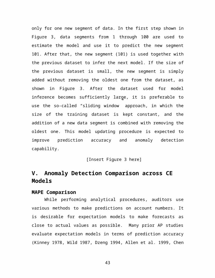
An important step when implementing continuous data level auditing is in determining which business process should be modeled by continuity equations and subject to AP testing. There are a large number of business processes that can be modeled—and as we have seen, far more data than can currently be handled—and the auditor cannot model all of them and indeed, does not need to. Providing assurance only necessitates the examination of the key processes that define a business, and these, in turn, will depend on the company’s strategy, its product space, competitive environment and current financial condition and history. There needs to be research undertaken on the general question of the types of business processes that an auditor is likely to encounter, and the way in which these processes can be represented in continuity equations.

VII Conclusion In this paper we develop a continuous data level auditing system

utilizing business process based analytical procedures. The first component of the system is automatic transaction verification to filter out exceptions, which are transactions violating user defined business process rules. The second component of the CA system uses continuity equations to provide benchmarks for process level AP tests which are applied to the transaction stream to identify statistical anomalies possibly indicating business process problems. AP tests are needed to complement transaction verification given the inability to define rules for all possible exceptions and to identify patterns of anomalous firm behavior.

This is the first study on the use of detailed data to develop analytical procedures for continuous auditing. It is also the first attempt to use empirical data to compare different AP models in a CA context. The choice of aggregation level in the AP tests is up to the auditor who is not constrained to use data that is already at a high

43

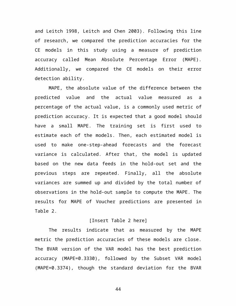
level of aggregation, such as account balances. Hence, the auditor has the freedom to make the tradeoff between utilizing more stable metrics by appropriate aggregation versus the resulting loss of information content, as opposed to being forced to accept limitation on the data imposed by outside circumstances. The highly disaggregated data that underlies CA allows auditors to fit equations relating to specific metrics, such as those related to individual business units, or individual customers or vendors, or small coherent subgroups of them. The main benefit, as compared with traditional analytical procedures is that anomalies can be identified which are undetectable at higher levels of aggregation.

We model flow relationships between different metrics of related business processes as a system of continuity equations. We use a seeded error simulation study to compare the anomaly detection capability of various CE models. Our results confirm that joint analysis of business processes gives the auditor an analytical procedure with a robust capability to detect anomalies in a real time continuous auditing environment with highly disaggregated data.

An important methodological innovation of this study is the examination of the capabilities of CA to investigate and correct identified problems in (close to) real time. We therefore introduce a real time error correction protocol in our simulation study and examine the differential detection capabilities between models with error correction and without error correction. We show that, as expected, under most circumstances the use of real time error correction results in superior performance.

Overall this study finds that while there are differences in the predictive ability and anomaly detection performance of various CE models, all models perform well and no single model performs better on all aspects. From this we can draw two important conclusions.

44

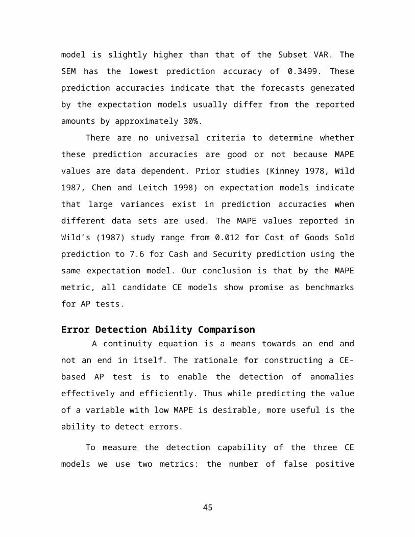
First, that unlike in the traditional audit literature on analytical procedures, the inability to choose a model across the candidate CE models is less important than the fact that all models yield efficient AP tests. The point is that because of its automated and technology driven nature, it is quite feasible and even desirable for the continuous data level audit system to use benchmarks based on multiple CE models instead of being forced to select only one, as would be necessary in a more manual system. For example, the BVAR model can be used first to detect anomalies because it has a low false negative error rate. Subsequently, the simultaneous equation model and the linear regression model can be used to remove the false alarms from the BVAR-detected anomalies because these two models have relatively low false positive error rates.

Our second conclusion from the fact that all the CE models yield reasonably effective analytical procedures is that when auditors have access to transaction data, the richness of that disaggregate data combined with the ability to make real time error correction makes error detection robust across a variety of expectations models. In other words, it is the nature of the data that serves as audit evidence that is the primary driver of audit effectiveness, with the selection of the specific analytical procedure a second order concern—not because the audit benchmark is not important, but because auditing at the process level makes errors stand out much more obviously in the data.

These are key conclusions in support of continuous data level auditing and its ability to make use of transaction data, implement real time error correction and give auditors the choice of the degree of aggregation. Future research on applying this CA methodology across different firms and different data sets is necessary to see whether these conclusions are robust, and to examine what their implications are for audit practice.

45

46

References:1. Allen R.D., M.S. Beasley, and B.C. Branson. 1999. Improving

Analytical Procedures: A Case of Using Disaggregate Multilocation Data, Auditing: A Journal of Practice and Theory 18 (Fall): 128-142.

2. Alles M.G., G. Brennan A. Kogan, and M.A. Vasarhelyi. 2006. Continuous Monitoring of Business Process Controls: A Pilot Implementation of a Continuous Auditing System at Siemens. International Journal of Accounting Information Systems, Volume 7, Issue 2 (June): 137-161.

3. Alles M.G., A. Kogan, and M.A Vasarhelyi. 2006b. Continuous Auditing: Lessons from Fifteen Years of Transforming Theory into Practice. Working paper, Rutgers Business School.

4. ____________________________________. 2002. Feasibility and Economics of Continuous Assurance. Auditing: A Journal of Practice and Theory 21 (Spring):125-138.

5. ____________________________________.2004. Restoring auditor credibility: tertiary monitoring and logging of continuous assurance systems. International Journal of Accounting Information Systems 5: 183-202.

6. Alles, M.G., A. Kogan, M.A. Vasarhelyi, and J.D. Warren. 2007. Continuous Auditing, A portfolio assembled for the Bureau of National Affairs. Washington, DC.

7. ____________________________________ and J. Wu. 2004. Continuity Equations: Business Process Based Audit Benchmarks in Continuous Auditing. Proceedings of American Accounting Association Annual Conference. Orlando, FL.

8. American Institute of Certified Public Accountants. 1988. Statement on Auditing Standards No. 56: Analytical Procedures. New York.

47

9. Auditing Concepts Committee of the American Accounting Association. 1972. Report of the committee on basic auditing concepts.

10. Bell T., F.O. Marrs, I. Solomon, and H. Thomas 1997. Monograph: Auditing Organizations Through a Strategic-Systems Lens. Montvale, NJ, KPMG Peat Marwick.

11. Biggs, S., T. Mock, and P Watkins. 1988. Auditors' use of analytical review in audit program design. The Accounting Review 63 (January): 148-161

12. Brown, Carol E. Jeffrey A. Wong, and Amelia A. Baldwin. 2006. Research Streams in Continuous Audit: A Review and Analysis of the Existing Literature. Collected Papers of the Fifteenth Annual Research Workshop on: Artificial Intelligence and Emerging Technologies in Accounting, Auditing and Tax. pp. 123-135. Washington, DC, USA, August 5, 2006.

13. Chen Y. and Leitch R.A. 1998. The Error Detection of Structural Analytical Procedures: A Simulation Study. Auditing: A Journal of Practice and Theory 17 (Fall): 36-70.

14. ______________________. 1999. An Analysis of the Relative Power Characteristics of Analytical Procedures. Auditing: A Journal of Practice and Theory 18 (Fall): 35-69.

15. CICA/AICPA. 1999. Continuous Auditing. Research Report, Toronto, Canada: The Canadian Institute of Chartered Accountants.

16. Davenport, T.H. and J.E. Short, 1990. The New Industrial Engineering: Information Technology and Business Process Redesign, Sloan Management Review, pp. 11-27, Summer.

17. Doan, T.A., Littleman R.B., and C.A. Sims. 1984. Forecasting and Conditional Projections Using Realistic Prior Distributions. Econometric Reviews 1, 1-100.

48

18. Dzeng S.C. 1994. A Comparison of Analytical Procedures Expectation Models Using Both Aggregate and Disaggregate Data. Auditing: A Journal of Practice and Theory 13 (Fall), 1-24.

19. Elliot, R.K. 2002. Twenty-First Century Assurance. Auditing: A Journal of Practice and Theory 21 (Spring), 129-146.

20. Enders, W. 2004. Applied Econometric Time Series. Second Edition. New York, NY: John Wiley and Sons.

21. Engle, R. 2001. GARCH 101: The Use of ARCH/GARCH model in Applied Econometrics. Journal of Economic Perspectives 15 (Fall): 157-168.

22. Felix, R.M. and L.C. Nunes. 2003. Forecasting Euro Area Aggregates with Bayesian VAR and VECM Models. Working Paper. Banco De Portugal. Economic Research Department.

23. Groomer, S.M. and U.S. Murthy. 1989. Continuous auditing of database applications: An embedded audit module approach. Journal of Information Systems 3 (2), 53-69.

24. Hammer, M. 1990. Reengineering Work: Don’t Automate, Obliterate! Harvard Business Review, Vol. 68, Issue 4 (July-August), 104-112.

25. Hentschel, L. 1995. All in the family Nesting symmetric and asymmetric GARCH models. Journal of Financial Economics 39 (1): 71-104.

26. Heston, S.L. and S. Nandi. 2000. A closed-form GARCH option valuation model. Review of Financial Studies 13: 585-625.

27. Hirst, E. and L. Koonce. 1996. Audit Analytical Procedures: A Field Investigation. Contemporary Accounting Research., Vol 13, No 2, Fall.

28. Hoitash, R. A. Kogan, and M.A. Vasarhelyi. 2006. Peer-Based Approach for Analytical Procedures. Auditing: A Journal of Practice and Theory Vol. 25, No.2 (November), 53–84.

49

29. Hylas, R. and R. Ashton. 1982. Audit detection of financial statement errors, The Accounting Review, Vol. 57 No.4, 751-65.

30. Kinney, W.R. 1978. ARIMA and Regression in Analytical Review: an Empirical Test. The Accounting Review, Vol. 17, No. 1, 148-165.

31. Kinney, W.R. and G.L. Salamon. 1982. Regression Analysis in Auditing: A Comparison of Alternative Investigation Rules. Journal of Accounting Research. Vol. 20. No. 2, 350-366.

32. Kinney, W.R.1987. Attention-Directing Analytical Review Using Accounting Ratios: A Case Study. Auditing: A Journal of Practice and Theory Vol. 6, No.2 (Spring), 59-73.

33. Knechel, W. R. 1988. The effectiveness of statistical analytical review as a substantive auditing procedure: A simulation analysis. The Accounting Review (January), 74-95.

34. Kogan, A. E.F. Sudit, and M.A. Vasarhelyi. 1999. Continuous Online Auditing: A Program of Research. Journal of Information Systems 13 (Fall), 87–103.

35. Koreisha, S. and Y. Fang. 2004. Updating ARMA Predictions for Temporal Aggregates. Journal of Forecasting 23, 275-396.

36. Lamoureux, C.G. and W. D. Lastrapes. 1990. Heteroskedasticity in Stock Return Data: Volume versus GARCH Effects. The Journal of Finance 45 (1), 221-229.

37. Leitch and Y. Chen. 2003. The Effectiveness of Expectation Models In Recognizing Error Patterns and Eliminating Hypotheses While Conducting Analytical Procedures. Auditing: A Journal of Practice and Theory 22 (Fall), 147-206.

38. Loebbecke, J. and P., Steinbart. 1987. An investigation of the use of preliminary analytical review to provide substantive

50

audit evidence, Auditing: A Journal of Practice and Theory, Vol. 6 No.2, 74-89.

39. Lorek, K.S., B.C. Branson, and R.C. Icerman. 1992. On the use of time-series models as analytical procedures. Auditing: A Journal of Practice & Theory, Vol. 11, No. 2 (Fall), 66-88.

40. Murthy, U.S. 2004. An Analysis of the Effects of Continuous Monitoring Controls on e-Commerce System Performance. Journal of Information Systems. 18 (Fall), 29–47.

41. ___________and M.S. Groomer. 2004. A continuous auditing web services model for XML-based accounting systems. International Journal of Accounting Information Systems 5, 139-163.

42. Murthy, U.S. and J.A. Swanson. 1992. Integrating Expert Systems and Database Technologies: An Intelligent Decision Support System For Investigating Cost Variances, Journal of Information Systems, 6(2) (Fall), 18-40.

43. Pandher G.S. 2002. Forecasting Multivariate Time Series with Linear Restrictions Using Unconstrained Structural State-space Models. Journal of Forecasting 21: 281-300.

44. Porter, M. E. 1996. What Is Strategy? Harvard Business Review, Vol. 74, #6, S. 6178.

45. PricewaterhouseCoopers. 2006. State of the internal audit profession study: Continuous auditing gains momentum. http://www.pwcglobal.com/images/gx/eng/about/svcs/grms/06_IAState_Profession_Study.pdf

46. Rezaee, Z., A. Sharbatoghlie, R. Elam, and P.L. McMickle. 2002. Continuous Auditing: Building Automated Auditing Capability. Auditing: A Journal of Practice and Theory 21 (Spring), 147-163.

47. Searcy, D. L., Woodroof, J. B., and Behn, B. 2003. Continuous Audit: The Motivations, Benefits, Problems, and Challenges

51

Identified by Partners of a Big 4 Accounting Firm. Proceedings of the 36th Hawaii International Conference on System Sciences: 1-10.

48. Stringer, K. and T. Stewart. 1986. Statistical techniques for analytical review in auditing. Wiley Publishing. New York.

49. Swanson, N., E. Ghysels, and M. Callan. 1999. A Multivariate Time Series Analysis of the Data Revision Process for Industrial Production and the Composite Leading Indicator. Book chapter of Cointegration, Causality, and Forecasting: Festchrift in Honour of Clive W.J. Granger. Eds. R. Engle and H. White. Oxford: Oxford University Press.

50. Vasarhelyi, M.A and F.B. Halper. 1991. The Continuous Audit of Online Systems. Auditing: A Journal of Practice and Theory 10 (Spring), 110–125.

51. _______________ 2002. Concepts in Continuous Assurance. Chapter 5 in Researching Accounting as an Information Systems Discipline, Edited by S. Sutton and V. Arnold. Sarasota, FL: AAA.

52. ______________, M. Alles, and A. Kogan. 2004. Principles of Analytic Monitoring for Continuous Assurance. Journal of Emerging Technologies in Accounting, Vol. 1, 1-21.

53. ______________, and M. Greenstein. 2003. Underlying principles of the electronization of business: A research agenda. International Journal of Accounting Information Systems 4: 1-25.

54. Vasarhelyi, Miklos A., Alles, M.G., Williams, K.T. Continuous Assurance for the Now Economy, A Thought Leadership Paper for the Institute of Chartered Accountants in Australia, forthcoming May 2010.

52

55. Wright, A. and R.H. Ashton. 1989. Identifying audit adjustments with attention-directing procedures. The Accounting Review (October), 710-28.

56. Woodroof, J. and D. Searcy 2001. Continuous Audit Implications of Internet Technology: Triggering Agents over the Web in the Domain of Debt Covenant Compliance. Proceedings of the 34th

Hawaii International Conference on System Sciences.57. Wu, J. Continuous Test of Details and Continuity

Equations in Continuous Audit, Ph.D Dissertation, Rutgers University, 2006.

53

Figures, Tables and Charts

Figure 1: Architecture of Data-Oriented Continuous Auditing System

54

Initial Model Estimation

Determine Parameter p-value threshold

Retain parameters below threshold; Restrict parameters over threshold to zero

Re-estimate Model

Do new parameter estimates all below threshold?

Final Model

Yes

No

Figure 2: Multivariate Time Series Model Selection

55

CA System

Data Segments for Analytical Modeling: 1,2,3,4,5,6……100

101102103101Predicted ValueAP Model 1

CA System

Data Segments for Analytical Modeling: 1,2,3,4,5,6……100, 101

102103104 102Predicted Value

AP Model 2

CA System

Data Segments for Analytical Modeling: 1,2,3,4,5,6……100, 101, 102

103104105 103Predicted Value

AP Model 3

Figure 3: Model Updating Protocol

Re-estimate Analytical Model

Re-estimate Analytical Model

56

Table 1: Summary Statistics

Variable N Mean Std Dev Minimum Maximum Order 180 10631.38 6840.51 4597 51392 Receive 180 8876.26 3195.16 4430 31412 Voucher 180 7496.74 3874.47 187 31209

The table presents the summary statistics for the transaction quantity daily aggregates for each business process. The low minimums for Receive and Voucher are due to the date cutting off problem. The data sets span from 10/01/03 to 06/30/04. Many related transactions for the Receive and Voucher for the first 2 days in the data sets may have happened before 10/01/03.

57

Table 2: MAPE Comparison among BVAR, Subset VAR, GARCH, SEM and Linear Regression Model: Prediction Accuracy for Daily Quantity Aggregate of Entire Company’s Vouchers

MAPE Std. Dev Min Max

BVAR 0.3330 0.3282 0.0008 1.5739

Subset VAR 0.3374 0.3210 0.0044 1.9180

SEM 0.3779 0.4403 0.0034 2.6275

LRM 0.3499 0.3677 0.0007 2.2481

GARCH 0.3461 0.3611 0.0007 2.1850

MAPE: Mean Absolute Percentage ErrorStd. Dev: Standard deviation for Absolute Percentage ErrorMin: The minimum value for Absolute Percentage ErrorMax: The maximum value for Absolute Percentage Error

58

Table 3: Error Rates Comparison between Error-correction and Non-correction Using Daily Quantity Aggregate Data , α=0.05

False Positive False Negative

ErrorMagnitude

Error Correction

Non-Correction

Error Magnitude

Error-Correction

Non-Correction

Bayesian

VAR

10% 0.342 0.336 10% 0.5500 0.550050% 0.339 0.328 50% 0.3750 0.4000100% 0.340 0.318 100% 0.2125 0.2500200% 0.344 0.293 200% 0.0625 0.1250400% 0.344 0.250 400% 0 0.0250

Subset

VAR

10% 0.039 0.039 10% 0.925 0.92550% 0.039 0.025 50% 0.825 0.825100% 0.039 0.014 100% 0.615 0.663200% 0.039 0.004 200% 0.212 0.350400% 0.039 0.002 400% 0.013 0.200

SEM 10% 0.1386 0.1386 10% 0.8125 0.812550% 0.1342 0.1200 50% 0.775 0.775100% 0.1412 0.1000 100% 0.425 0.425200% 0.1400 0.0629 200% 0.1875 0.25400% 0.1331 0.0286 400% 0.025 0.1125

LRM 10% 0.09 0.09 10% 0.8625 0.862550% 0.089 0.0643 50% 0.8125 0.8125100% 0.089 0.0457 100% 0.525 0.6125200% 0.09 0.0286 200% 0.1875 0.2875400% 0.09 0.02 400% 0.0125 0.175

GARCH

10% 0.0875 0.0875 10% 0.8625 0.862550% 0.0861 0.0583 50% 0.8125 0.8125100% 0.0861 0.0431 100% 0.525 0.6125200% 0.0875 0.0264 200% 0.1875 0.2875400% 0.0875 0.0194 400% 0.0125 0.1625

59

Table 4: False Negative Error Rates Comparisons (Weekly, Weekly Best Case, Weekly Worst Case)

Error Magnit

ude

Weekly Aggregation

Weekly Aggregation

Best Case

Weekly AggregationWorst Case

Error-Correcti

on

Non-Correcti

on

Error-Correcti

on

Non-Correcti

on

Error-Correcti

on

Non-Correcti

onBVAR 10% 0.650 0.675 0.3 0.3 0.650 0.635

50% 0.125 0.200 0 0 0.350 0.555100% 0.025 0.150 0 0 0.070 0.485200% 0 0.050 0 0 0.025 0.535400% 0 0.025 0 0 0.055 0.675

Subset

VAR

10% 0.800 0.800 0.925 0.925 0.945 0.94550% 0.425 0.500 0 0.025 0.885 0.890

100% 0.050 0.300 0 0 0.615 0.725200% 0 0.150 0 0 0.035 0.320400% 0 0.175 0 0 0.025 0.180

SEM 10% 0.850 0.850 0.875 0.875 0.860 0.86050% 0.100 0.200 0 0.025 0.810 0.810

100% 0.050 0.050 0 0 0.255 0.500200% 0 0.050 0 0 0.030 0.155400% 0 0.050 0 0 0.025 0.035

LRM 10% 0.900 0.900 0.925 0.925 0.915 0.91550% 0.175 0.625 0 0.025 0.855 0.87

100% 0.025 0.225 0 0 0.435 0.64200% 0 0.075 0 0 0.035 0.24400% 0 0.050 0 0 0.025 0.09

GARCH

10% 0.9 0.9 0.8 0.8 0.915 0.91550% 0.175 0.65 0.025 0.025 0.805 0.835

100% 0.05 0.275 0 0.025 0.43 0.565200% 0 0.075 0 0 0.015 0.185400% 0 0.075 0 0 0.015 0.045

60

Figure 4: BVAR Model Comparisons

A. BVAR Model False Positive Rate Comparisons (Entire firm, Subunit Best Case, Subunit Worst Case)

0.15

0.20

0.25

0.30

0.35

0.40

0% 100% 200% 300% 400%

Error Magnitude

False

Pos

itive

Erro

r Rat

es

Entire-EC

Entire-NCBest-EC

Best-NCWorst-EC

Worst-NC

B. BVAR Model False Negative Rate Comparisons (Entire firm, Subunit Best Case, Subunit Worst Case)

-0.10

0.00

0.10

0.20

0.30

0.40

0.50

0.60

0.70

0.80

0% 100% 200% 300% 400%

Error Magnitude

False

Neg

ativ

e Er

ror R

ates

Entire-EC

Entire-NC

Best-EC

Best-NC

Worst-EC

Worst-NC

Entire-EC: Error correction model using entire company dataEntire-NC: Non-correction model using entire company dataBest-EC: Error correction model using mean subunit best case scenario dataBest-NC: Non-correction model using mean subunit best case scenario dataWorst-EC: Error correction model using mean subunit worst case scenario dataWorst-NC: Non-Error correction model using mean subunit worst case scenario data

61