FINAL PROJECT REPORT YEAR: 2013

WTFRC Project Number: TR-10-110

Project Title: High resolution weather forecasting for freeze prediction in WA

PI: Gerrit Hoogenboom Co-PI: Tesfamichael Ghidey

Organization: Washington State University Organization: Washington State University

Telephone: 509-786-9371 Telephone: 509-786-9299

Email: gerrit.hoogenboom@wsu.edu Email: t.ghidey@wsu.edu

Address: AgWeatherNet Address: AgWeatherNet

Address 2: 24106 North Bunn Road Address 2: 24106 North Bunn Road

City/State/Zip: Prosser, WA 99350-8694 City/State/Zip: Prosser, WA 99350-8694

Co-PI: Heping Liu Co-PI: Nic Loyd

Organization: Washington State University Organization: Washington State University

Telephone: 509-335-1529 Telephone: 509-786-9357

Email: heping.liu@wsu.edu Email: Nicholas.loyd@wsu.edu

Address: Lab for Atmospheric Research Address: AgWeatherNet

Address 2: Dept. of Civil and Env Eng Address2: 24106 North Bunn Road

City/State/Zip: Pullman, WA 99164 City/State/Zip: Prosser, WA 99350-8694

Cooperators: None

Total Project Request: Year 1: $90,000 Year 2: Not Funded Year 3: Not Funded

Percentage time per crop: Apple: 50% Pear: 10% Cherry: 30% Stone Fruit: 10%

Other funding sources

Indirect support through the existing infrastructure of AgWeatherNet and its 151 weather stations

WTFRC Collaborative expenses: NONE

Organization Name: CAHNRS- WSU Contract Administrator: Carrie Johnston

Telephone: 509-335-4564 Email address: carriej@wsu.edu

Item 2013 2014 2015

Salaries 56,361

Benefits 22,588

Wages

Benefits

Equipment

Supplies 10,051

Travel 1,000

Miscellaneous

Plot Fees

Total 90,000 Not funded Not funded Footnotes: The budget requested includes support for a Postdoctoral Research Associate who will be responsible for

evaluation and implementation of the Weather Research and Forecasting (WRF) model for three years. We also have

requested partial support for an application programmer for integration of the WRF model outputs with the web site of

AgWeatherNet (www.weather.wsu.edu), integration with various models and overall information delivery. Additional

budget items include operating expenses for computer software, additional harddisk storage, and related costs and travel to

participate in meetings with producers and stakeholders and workshops on the WRF modeling system.

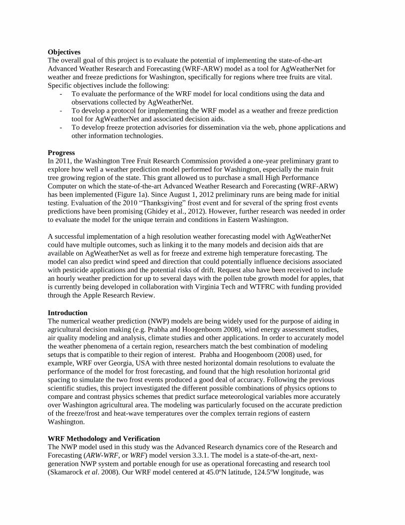
Objectives

The overall goal of this project is to evaluate the potential of implementing the state-of-the-art

Advanced Weather Research and Forecasting (WRF-ARW) model as a tool for AgWeatherNet for

weather and freeze predictions for Washington, specifically for regions where tree fruits are vital.

Specific objectives include the following:

- To evaluate the performance of the WRF model for local conditions using the data and

observations collected by AgWeatherNet.

- To develop a protocol for implementing the WRF model as a weather and freeze prediction

tool for AgWeatherNet and associated decision aids.

- To develop freeze protection advisories for dissemination via the web, phone applications and

other information technologies.

Progress

In 2011, the Washington Tree Fruit Research Commission provided a one-year preliminary grant to

explore how well a weather prediction model performed for Washington, especially the main fruit

tree growing region of the state. This grant allowed us to purchase a small High Performance

Computer on which the state-of-the-art Advanced Weather Research and Forecasting (WRF-ARW)

has been implemented (Figure 1a). Since August 1, 2012 preliminary runs are being made for initial

testing. Evaluation of the 2010 “Thanksgiving” frost event and for several of the spring frost events

predictions have been promising (Ghidey et al., 2012). However, further research was needed in order

to evaluate the model for the unique terrain and conditions in Eastern Washington.

A successful implementation of a high resolution weather forecasting model with AgWeatherNet

could have multiple outcomes, such as linking it to the many models and decision aids that are

available on AgWeatherNet as well as for freeze and extreme high temperature forecasting. The

model can also predict wind speed and direction that could potentially influence decisions associated

with pesticide applications and the potential risks of drift. Request also have been received to include

an hourly weather prediction for up to several days with the pollen tube growth model for apples, that

is currently being developed in collaboration with Virginia Tech and WTFRC with funding provided

through the Apple Research Review. Introduction The numerical weather prediction (NWP) models are being widely used for the purpose of aiding in

agricultural decision making (e.g. Prabha and Hoogenboom 2008), wind energy assessment studies,

air quality modeling and analysis, climate studies and other applications. In order to accurately model

the weather phenomena of a certain region, researchers match the best combination of modeling

setups that is compatible to their region of interest. Prabha and Hoogenboom (2008) used, for

example, WRF over Georgia, USA with three nested horizontal domain resolutions to evaluate the

performance of the model for frost forecasting, and found that the high resolution horizontal grid

spacing to simulate the two frost events produced a good deal of accuracy. Following the previous

scientific studies, this project investigated the different possible combinations of physics options to

compare and contrast physics schemes that predict surface meteorological variables more accurately

over Washington agricultural area. The modeling was particularly focused on the accurate prediction

of the freeze/frost and heat-wave temperatures over the complex terrain regions of eastern

Washington.

WRF Methodology and Verification

The NWP model used in this study was the Advanced Research dynamics core of the Research and

Forecasting (ARW-WRF, or WRF) model version 3.3.1. The model is a state-of-the-art, next-

generation NWP system and portable enough for use as operational forecasting and research tool

(Skamarock et al. 2008). Our WRF model centered at 45.0ºN latitude, 124.5ºW longitude, was

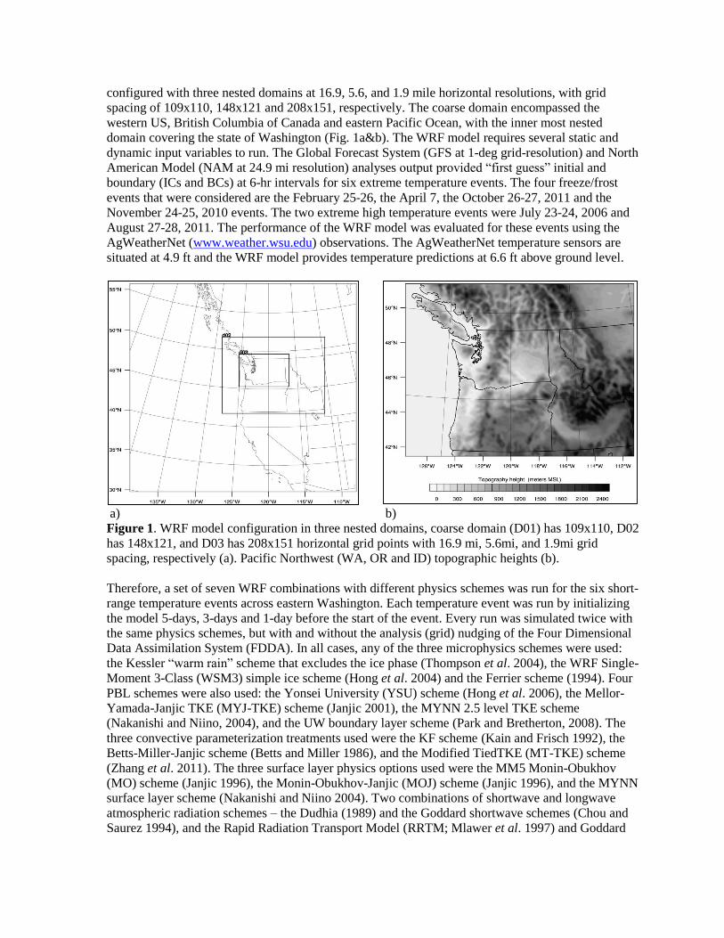
configured with three nested domains at 16.9, 5.6, and 1.9 mile horizontal resolutions, with grid

spacing of 109x110, 148x121 and 208x151, respectively. The coarse domain encompassed the

western US, British Columbia of Canada and eastern Pacific Ocean, with the inner most nested

domain covering the state of Washington (Fig. 1a&b). The WRF model requires several static and

dynamic input variables to run. The Global Forecast System (GFS at 1-deg grid-resolution) and North

American Model (NAM at 24.9 mi resolution) analyses output provided “first guess” initial and

boundary (ICs and BCs) at 6-hr intervals for six extreme temperature events. The four freeze/frost

events that were considered are the February 25-26, the April 7, the October 26-27, 2011 and the

November 24-25, 2010 events. The two extreme high temperature events were July 23-24, 2006 and

August 27-28, 2011. The performance of the WRF model was evaluated for these events using the

AgWeatherNet (www.weather.wsu.edu) observations. The AgWeatherNet temperature sensors are

situated at 4.9 ft and the WRF model provides temperature predictions at 6.6 ft above ground level.

a) b)

Figure 1. WRF model configuration in three nested domains, coarse domain (D01) has 109x110, D02

has 148x121, and D03 has 208x151 horizontal grid points with 16.9 mi, 5.6mi, and 1.9mi grid

spacing, respectively (a). Pacific Northwest (WA, OR and ID) topographic heights (b).

Therefore, a set of seven WRF combinations with different physics schemes was run for the six short-

range temperature events across eastern Washington. Each temperature event was run by initializing

the model 5-days, 3-days and 1-day before the start of the event. Every run was simulated twice with

the same physics schemes, but with and without the analysis (grid) nudging of the Four Dimensional

Data Assimilation System (FDDA). In all cases, any of the three microphysics schemes were used:

the Kessler “warm rain” scheme that excludes the ice phase (Thompson et al. 2004), the WRF Single-

Moment 3-Class (WSM3) simple ice scheme (Hong et al. 2004) and the Ferrier scheme (1994). Four

PBL schemes were also used: the Yonsei University (YSU) scheme (Hong et al. 2006), the Mellor-

Yamada-Janjic TKE (MYJ-TKE) scheme (Janjic 2001), the MYNN 2.5 level TKE scheme

(Nakanishi and Niino, 2004), and the UW boundary layer scheme (Park and Bretherton, 2008). The

three convective parameterization treatments used were the KF scheme (Kain and Frisch 1992), the

Betts-Miller-Janjic scheme (Betts and Miller 1986), and the Modified TiedTKE (MT-TKE) scheme

(Zhang et al. 2011). The three surface layer physics options used were the MM5 Monin-Obukhov

(MO) scheme (Janjic 1996), the Monin-Obukhov-Janjic (MOJ) scheme (Janjic 1996), and the MYNN

surface layer scheme (Nakanishi and Niino 2004). Two combinations of shortwave and longwave

atmospheric radiation schemes – the Dudhia (1989) and the Goddard shortwave schemes (Chou and

Saurez 1994), and the Rapid Radiation Transport Model (RRTM; Mlawer et al. 1997) and Goddard

longwave schemes (Chou and Saurez 1994) – were also used. Table 1 shows a summary of the

physics options that were used in our study.

Table 1. Physics schemes used for WRF configuration (numbers are WRF name-list codes). Microphysics

schemes

Planetary

Boundary

Layer (PBL)

Surface

Layer

Cumulus

Parameterization

s schemes

Shortwave

Atmospheric

Radiation

Longwave

Atmospheric

Radiation

1. Ferrier, 5 MYJ-tke, 2 MO, 1 BMJ, 2 Dudhia, 1 RRTM, 1

2. Kessler, 1 MYNN, 5 MOJ, 2 KF, 1 Godard, 5 Godard, 5

3. WSM3, 3 UW BL, 9 MYNN, 5 MT-tke, 6

4. YSU, 1

The statistical methods used include: the Mean Bias (MB, has a unit), the Normalized Mean Bias

(NMB, in %), the Root Mean Square Error (RMSE, has a unit), the Correction Coefficient (r, unitless)

with its Coefficient of Determination (r2, %) and the Skill Score (SS, unitless), as defined below.

𝑀𝐵 =1

𝑛∑ (𝑃𝑖−𝑂𝑖)𝑛

𝑖=1 ; 𝑁𝑀𝐵 = ∑ (𝑃𝑖−𝑂𝑖)𝑛

𝑖=1

∑ 𝑂𝑖𝑛𝑖=1

. 100 (1)

𝑅𝑀𝑆𝐸 = √1

𝑛∑ (𝑃𝑖 − 𝑂𝑖)2𝑛

𝑖=1 ; 𝑟 = ∑ (𝑂𝑖−𝑂).(𝑃𝑖−𝑃)𝑛

𝑖=1

√∑ (𝑂𝑖−𝑂)2𝑛𝑖=1 .∑ (𝑃𝑖−𝑃)2𝑛

𝑖=1

(2)

𝑆𝑆 = 1 − 𝑀𝑆𝐸(𝑃,𝑂)

𝑀𝑆𝐸(𝑂,𝑂) (3)

Where,

𝑀𝑆𝐸(𝑃, 𝑂) = 1

𝑛∑ (𝑃𝑖 − 𝑂𝑖)2𝑛

𝑖=1 , & 𝑀𝑆𝐸(𝑂, 𝑂) = 1

𝑛∑ (𝑂 − 𝑂𝑖)2𝑛

𝑖=1 .

𝑃𝑖 & 𝑂𝑖 are, respectively, WRF predicted and observed meteorological parameters (e.g., temperature),

where i represents a given time and/or station location with a total number of n samples. The averages

of forecast results and observations are also defined, respectively, as: 𝑃 = ∑ 𝑃𝑖𝑛𝑖=1 & 𝑂 = ∑ 𝑂𝑖

𝑛𝑖=1 .

The coefficient of determination is the square of the correction coefficient (r2). Murphy (1988) has

defined skill scores as measures of the relative accuracy of forecasts produced by two forecasting

systems, one of which is “reference system”. He has also defined accuracy as the average degree of

association between individual forecasts and observations, in which it’s mainly represented by the

mean absolute error. Referring to equation (5) above, the skill score (SS) can be positive (negative)

when the accuracy of the forecasts is greater (less) than the accuracy of the reference forecasts. SS =1

when MSE(P,O) = 0 implying a perfect forecast, and SS = 0 when MSE(P,O) = 𝑀𝑆𝐸(𝑂, 𝑂).

Table 2. Combination of configured physics schemes utilized in running the WRF model.

RUNS Microphysics

schemes

Planetary

Boundary

Layer (PBL)

Surface

Layer

Cumulus

Parameterizations

schemes

SW

Atmospheric

Radiation

LW

Atmospheric

Radiation

FDDA

grid

nudging

Run1 Ferrier MYNN MO MT-tke Godard Godard No

Run2 Ferrier MYNN MO MT-tke Godard Godard Yes

Run3 Ferrier UW BL MO MT-tke Dudhia Dudhia No

Run4 Ferrier UW BL MO MT-tke Dudhia Dudhia Yes

Run5 Kessler MYJtke MOJ BMJ Dudhia Dudhia No

Run6 Kessler MYJtke MOJ BMJ Dudhia Dudhia Yes

Run7 Kessler UW BL MYNN BMJ Godard Godard No

Run8 Kessler UW BL MYNN BMJ Godard Godard Yes

Run9 WSM3 YSU MO KF Dudhia Dudhia No

Run10 WSM3 YSU MO KF Dudhia Dudhia Yes

Run11 WSM3 MYNN MYNN KF Godard Godard No

Run12 WSM3 MYNN MYNN KF Godard Godard Yes

Run13 WSM3 MYJtke MOJ KF Dudhia Dudhia No

Run14 WSM3 MYJtke MOJ KF Dudhia Dudhia Yes

Results

A number of experiments with different physics schemes and numerical option tests were conducted.

These included the use of two large scale “first guess” analyses for model ICs and BCs, nested

domain horizontal resolutions, compatible combinations of physics schemes and the use of FDDA

grid (analysis) nudging at time intervals of the BCs input data for the coarser domains.

1. Impact of Large Scale Analyses as “first guess” Input

Two large scale “first guess” analyses were conducted to identify the model input data that provides

the most accurate ICs and BCs for simulation. The NCEP GFS final and NAM were used to analyze

the “Thanksgiving deep freeze” of 24-25 November 2010 and the summertime heat wave of 27-28

August 2011. To perform this test, one set of physics options (referred to as ‘Run1’ in Table 2) was

implemented. For each event, three runs initialized at different days were performed, in which the

model was initialized starting 5-days, 3-days and 1-day before the actual weather phenomena had

occurred. Moreover, the runs were also repeated to include the FDDA analysis nudging in the first

two coarser domains, bringing the total sum of simulations to six.

For the deep freeze of 24-25 November 2010, the model was unable to capture the low temperature

patterns for both input data: NAM with overall 24-hr mean biases of 22.0oF, 22.7oF and 14.8oF for the

5-day, 3-day, and 1-day initializations, and FNL with daily mean biases of 23.2oF, 23.2oF and 14.4oF,

respectively (Table 3). And hence the NAM initialized model results were slightly better than the

ones from FNL data. During this event most stations recorded close to -4oF, in that the WRF model

was unable to capture the phenomenon. WRF, however, performed better for the 27-28 August 2011

extreme warm case. The daily MBs for WRF from NAM (FNL) were estimated to be -5.4oF (-4.7) for

the 5-day, -5.0oF (-4.1) for the 3-day, and -0.4oF (-1.4) for the 1-day model initialization before the

event day. For the August case study the WRF model forecasted slightly better when it was initialized

with the FNL than NAM data. The MB results were similarly supported by the RMSE values as

shown in Table 3. Another measuring parameter of model performance is the skill score (SS), in

which the values close to one are the best skill to forecast more accurately (see Table 3). The SS

showed clearly a better performance of the NAM “first guess” data for November at -10.1 (Vs. -11.5

from FNL), while FNL performed better for the August case at -0.2 (Vs. -0.4 from NAM) for the 5-

day run. Interestingly, when analysis (grid) nudging method was switched on in the simulations of

both cases, the SS showed that FNL performed better than NAM for the November (0.2 vs. 0.3) and

the August (0.3 vs. 0.5) cases. The use of FNL data also showed better WRF performance than NAM

in other cases.

Table 3. Statistical results of NAM- and FNL-initialized WRF runs.

NAM-Initialized FNL-Initialized

Run1 Run2-FDDA Run1 Run2-FDDA 5-

day

3-

day 1-

day 5-

day

3-

day 1-

day 5-

day

3-

day 1-

day 5-

day

3-

day 1-

day

24-25

Nov

2010

RMSE (oF) 22.7 23.6 15.5 5.9 5.6 5.0 24.1 23.9 15.5 6.1 5.9 5.2

MB (oF) 22.0 22.7 14.8 4.7 4.3 3.6 23.2 23.2 14.4 4.5 4.1 3.4

S-score -10.0 -11.1 -4.1 0.3 0.3 0.5 -11.5 -11.5 -4.1 0.2 0.3 0.1

R2 36 28 50 76 75 76 29 27 36 68 68 57

RMSE (oF) 7.7 7.6 5.2 4.9 4.9 4.9 7.4 6.8 5.2 5.6 5.6 5.6

MB (oF) -5.4 -5.0 -0.4 -0.5 -0.4 -0.2 -4.7 -4.1 -1.4 -1.6 -1.6 -1.4

27-28

Aug

2011

S-score -0.4 -0.1 0.4 0.5 0.5 0.5 -0.2 0.3 0.4 0.3 0.3 0.3

R2

53 61 63 63 62 63 58 59 64 59 59 59

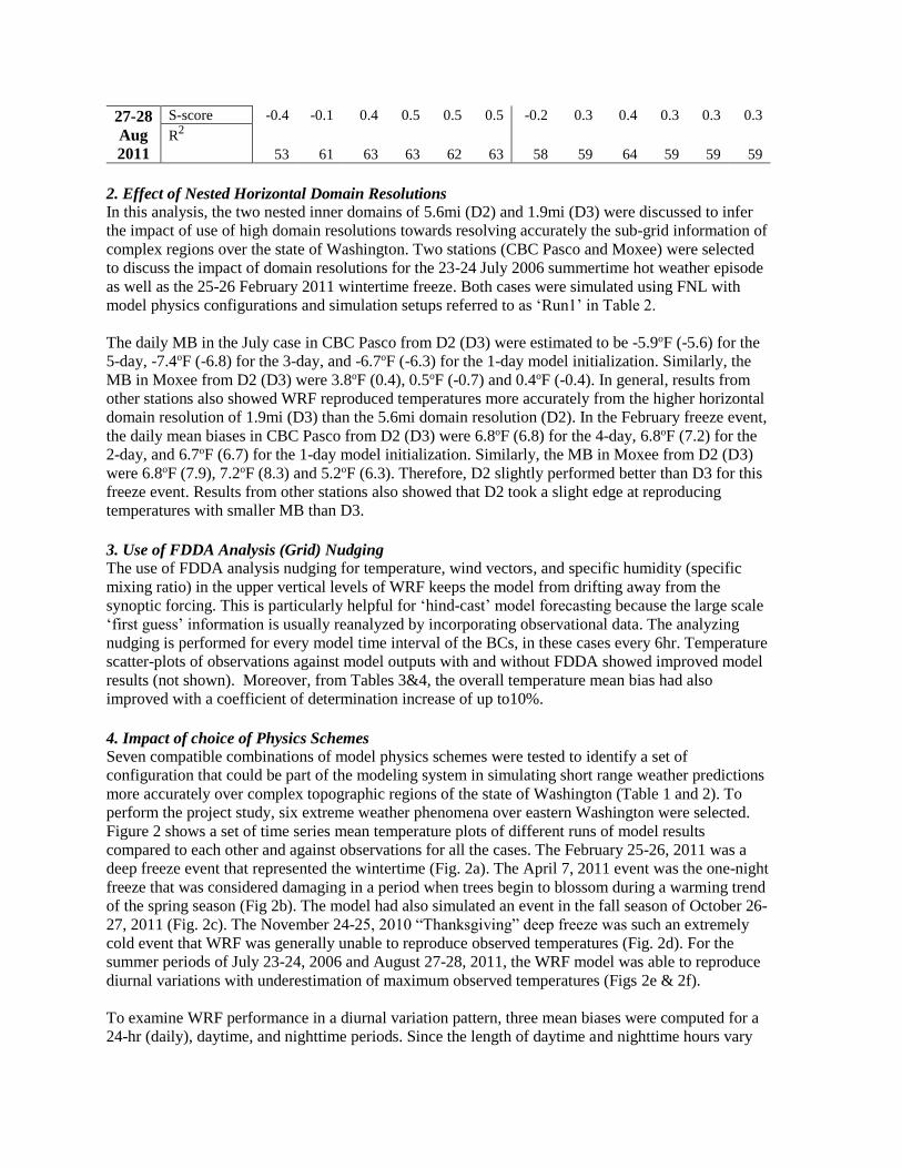
2. Effect of Nested Horizontal Domain Resolutions

In this analysis, the two nested inner domains of 5.6mi (D2) and 1.9mi (D3) were discussed to infer

the impact of use of high domain resolutions towards resolving accurately the sub-grid information of

complex regions over the state of Washington. Two stations (CBC Pasco and Moxee) were selected

to discuss the impact of domain resolutions for the 23-24 July 2006 summertime hot weather episode

as well as the 25-26 February 2011 wintertime freeze. Both cases were simulated using FNL with

model physics configurations and simulation setups referred to as ‘Run1’ in Table 2.

The daily MB in the July case in CBC Pasco from D2 (D3) were estimated to be -5.9oF (-5.6) for the

5-day, -7.4oF (-6.8) for the 3-day, and -6.7oF (-6.3) for the 1-day model initialization. Similarly, the

MB in Moxee from D2 (D3) were 3.8oF (0.4), 0.5oF (-0.7) and 0.4oF (-0.4). In general, results from

other stations also showed WRF reproduced temperatures more accurately from the higher horizontal

domain resolution of 1.9mi (D3) than the 5.6mi domain resolution (D2). In the February freeze event,

the daily mean biases in CBC Pasco from D2 (D3) were 6.8oF (6.8) for the 4-day, 6.8oF (7.2) for the

2-day, and 6.7oF (6.7) for the 1-day model initialization. Similarly, the MB in Moxee from D2 (D3)

were 6.8oF (7.9), 7.2oF (8.3) and 5.2oF (6.3). Therefore, D2 slightly performed better than D3 for this

freeze event. Results from other stations also showed that D2 took a slight edge at reproducing

temperatures with smaller MB than D3.

3. Use of FDDA Analysis (Grid) Nudging

The use of FDDA analysis nudging for temperature, wind vectors, and specific humidity (specific

mixing ratio) in the upper vertical levels of WRF keeps the model from drifting away from the

synoptic forcing. This is particularly helpful for ‘hind-cast’ model forecasting because the large scale

‘first guess’ information is usually reanalyzed by incorporating observational data. The analyzing

nudging is performed for every model time interval of the BCs, in these cases every 6hr. Temperature

scatter-plots of observations against model outputs with and without FDDA showed improved model

results (not shown). Moreover, from Tables 3&4, the overall temperature mean bias had also

improved with a coefficient of determination increase of up to10%.

4. Impact of choice of Physics Schemes

Seven compatible combinations of model physics schemes were tested to identify a set of

configuration that could be part of the modeling system in simulating short range weather predictions

more accurately over complex topographic regions of the state of Washington (Table 1 and 2). To

perform the project study, six extreme weather phenomena over eastern Washington were selected.

Figure 2 shows a set of time series mean temperature plots of different runs of model results

compared to each other and against observations for all the cases. The February 25-26, 2011 was a

deep freeze event that represented the wintertime (Fig. 2a). The April 7, 2011 event was the one-night

freeze that was considered damaging in a period when trees begin to blossom during a warming trend

of the spring season (Fig 2b). The model had also simulated an event in the fall season of October 26-

27, 2011 (Fig. 2c). The November 24-25, 2010 “Thanksgiving” deep freeze was such an extremely

cold event that WRF was generally unable to reproduce observed temperatures (Fig. 2d). For the

summer periods of July 23-24, 2006 and August 27-28, 2011, the WRF model was able to reproduce

diurnal variations with underestimation of maximum observed temperatures (Figs 2e & 2f).

To examine WRF performance in a diurnal variation pattern, three mean biases were computed for a

24-hr (daily), daytime, and nighttime periods. Since the length of daytime and nighttime hours vary

during a day from winter to summer seasons, a daytime in this study was defined as the time between

0800 – 1600 totaling nine hours and nighttime between 0000 – 0700 and 1700 – 2300 with a total of

15 hours were used for the period October – April. Between May – September, daytime was defined

between the hours of 0700 – 1900, while the nighttime between 0000-0060 and 2000 – 2300.

(a) (b)

(c) (d)

(e) (f)

Figure 2. WRF output temperature results from seven physics configured schemes (labeled with

color lines) against their corresponding station-average observations for the six cases. February 23-

28, 2011 (a). April 5-9, 2011 (b). October 23-29, 2011 (c). November 21-28, 2010 (d). July 20-26,

2006 (e). August 24-29, 2011 (f). These runs were initialized 2-3 days ahead of the weather event

date.

The results from the highest horizontal domain resolution of 1.9mi (D3) for 14 WRF runs were

individually compared with their corresponding AgWeatherNet observations. The qualitative

statistical plots (histograms) show the three categories of the diurnal variations: the daily, daytime and

nighttime, averaged over all available stations. These histogram plots depict the temperature MB in a

color-coded various model results. Table 4 also contains additional details of the daily statistical

estimates of RMSE, NMB, SS and ‘r’. Whereas the model runs with odd-numbers (Run 1-13) show

the seven configured WRF runs, their consecutive even-numbers (Run 2-14) represent results from

WRF-FDDA simulations.

The February 25-26, 2011 freeze event temperature MB estimates over 134 stations showed an over

prediction (Figure 3). The model configurations used in ‘Run13’ predicted observed temperatures

better with MB of 4.5oF, RMSE of 5.6oF and daily SS of -0.3 (Table 4). For WRF-FDDA runs,

‘Run10’ (the clone of ‘Run9’) reproduced observations most accurately. The April 7 MB estimate

over the 134 stations showed that ‘Run3’ scored the least daily MB (-0.2oF), (Fig. 3b). Based on the

RMSE estimate, the ‘Run9’ predicted most accurately at 5.2oF. ‘Run9’ scored the daily SS of -1.6, as

the best value (Table 4). The October 26-27 RMSE over 136 stations showed that ‘Run11’ performed

better with a value of 6.8oF (Fig. 3c). However, the daily skill score (at SS = -2.0) indicated that

‘Run9’ performed well. When WRF-FDDA runs were considered, ‘Run10’ (the clone of ‘Run9’)

reproduced observed values most accurately with the least MB, RMSE and SS (Table 4). As was

shown in the previous subsection for the November 24-25, 2010 ‘Thanksgiving’ deep freeze, all

statistics also showed that all model setups for the simulations had significantly overestimated

temperature observations during both day- and night-time periods with an average error of 21.6oF

calculated over 134 stations (Fig. 3d). ‘Run13’ had the least MB and RMSE estimates. Its skill score

also showed that the model’s accuracy relative to the reference system of average observations was

too far apart and hence drew the lowest magnitude. However, the FDDA method influenced the WRF

model strongly for all model setups (Table 4).

During the heat wave event of July 23, 2006, maximum mean temperature over the 44 AgWeatherNet

stations averaged at 101.7oF (Fig. 2e). Figure 3e shows that ‘Run1’ performed better in predicting

observed temperatures with the least MB value of -4.1oF. Likewise, the RMSE (6.5oF), SS (0.2),

NMB (-5%) and the ‘r’ (0.82) for this event had also supported the lowest errors computed from

‘Run1’ (Table 4). From the WRF-FDDA results, ‘Run2’ (the clone of ‘Run1’) also reproduced

observed values. In the case of ‘Run2’, the use of FDDA method did worsen errors as the event was

more influenced by local effects of the sub-grid processes rather than the synoptic large scale effects.

In Figure 3e, we can also observe that the largest errors came from daytime as WRF underestimated

maximum temperatures due to the strong effects of subsidence heating. For the extreme high

temperature event of August 27-28, 2011, the average maximum temperature over 136 stations was

91.8oF on August 27 (Fig. 2f). The scheme in ‘Run1’ performed better in predicting observed

temperatures with MB value of -4.1oF. The RMSE (6.8oF), SS (-0.1), NMB (-5%) and the ‘r’ (0.78)

estimates also supported MB results (Table 4). The use of FDDA in ‘Run2’ also reduced the errors.

(a) (b)

(c) (d)

(e) (f)

Figure 3. WRF output temperature Mean Bias over all available stations for seven physics configured

schemes (deep colored lines with odd numbers) and their corresponding FDDA-incorporated runs

(light colored lines with even numbers). February 25-26, 2011 (a). April 7, 2011 (b). October 26-27,

2011 (c). November 26-27, 2010 (d). July 23-24, 2006 (e). August 27-28, 2011 (f).

Table 4. WRF temperature statistical results against available AgWeatherNet stations for Feb, Apr,

Oct, Nov, Jul and Aug of the studied events (bold digits are best results).

WRF

Runs

25-26 Feb 2011 | 7 Apr 2011 | 26-27 Oct 2011 | 24-25 Nov 2010 | 23-24 Jul 2006 | 27-28 Aug

2011

RMSE (oF) MB (oF) NMB SS Corr. Coef. (r)

Run1 7.2 | 5.8 | 8.1 |

23.9 | 6.5 | 6.8

6.8 | -0.5 | 6.8 |

23.2 | -4.1 | -4.1

47 | -1 | 19 |

166 | -5 | -5

-1.3 | -2.0 | -2.7 |

-11.5 | 0.2 | -0.1

0.81 | 0.25 | 0.41 |

0.50 | 0.82 | 0.78

Run2 4.7 | 5.6 | 7.7 |

5.9 | 6.8 | 5.6

3.4 | -0.5 | 6.1 |

4.1 | -4.5 | -1.6

25 | -1 | 17 |

26 | -5 | -2

0.1 | -1.9 | -2.4 |

0.3 | 0.0 | 0.3

0.83 | 0.27 | 0.37 |

0.82 | 0.78 | 0.76

Run3 7.7 | 6.1 | 7.7 |

22.9 | 8.3 | 7.7

7.0|-0.2 | 6.3 |

22.0 | -6.8 | -5.6

48 | 1 | 18 |

156 | -8 | -7

-1.3 | -2.4 | -2.4 |

-10.1 | -0.5 | -0.4

0.81 | 0.18 | 0.45 |

0.49 | 0.78 | 0.75

Run4 4.7 | 5.8 | 7.2 |

13.5 | 8.5 | 6.1

3.2 | -0.5 | 5.2 |

12.6 | -6.3 | -3.4

25 | 0.2 | 15 |

84 | -7 | -4

0.2 | -2.1 | -1.9 |

-3.0 | -0.5 | 0.1

0.83 | 0.24 | 0.40 |

0.58 | 0.76 | 0.79

Run5 7.4 | 6.5 | 7.6 |

21.8 | 14.9 | 9.0

6.5 |-3.1 | 4.0 |

20.9 | -13.3 | -6.3

49 | -5 | 13 |

147 | -15 | -7

-1.2 | -1.6 | -2.6 |

-9.0 | -2.3| -1.0

0.78 | 0.43 | 0.48 |

0.56 | 0.53 | 0.73

Run6 4.9 | 5.8 | 7.2 |

13.5 | 9.5 | 7.7

3.1 | -1.6 | 4.7 |

13.2 | -6.8 | -3.4

25 | -2 | 14 |

83 | -7 | -4

0.1 | -2.1 | -2.2 |

-2.9 | -0.9 | -0.4

0.81 | 0.39 | 0.42 |

0.58 | 0.74 | 0.77

Run7 8.5 | 6.3 | 7.2 |

23.6 | 10.3 | 7.9

7.7 | -0.9 | 5.0 |

22.9 | -8.8 | -5.2

55 | -1 | 15 |

161 | -10 | -6

-1.8 | -2.6 | -2.3 |

-10.8 | -1.2 | -0.4

0.73 | 0.26 | 0.49 |

0.47 | 0.76 | 0.70

Run8 5.0 | 6.5 | 7.0 |

14.4 | 7.4 | 5.6

3.6 | -1.6 | 5.4 |

13.0 | -5.0 | -2.2

27 | -2 | 15 |

89 | -6 | -3

0.01 | -3.1 | -2.0 |

-3.3 | -0.1 | 0.3

0.80 | 0.22 | 0.41 |

0.54 | 0.76 | 0.78

Run9 6.7 | 5.2 | 7.2 |

19.8 | 8.3 | 7.7

5.8 | -0.7 | 5.8 |

18.9 | -6.7 | -5.4

42 | -2 | 16 |

135 | -8 | -7

-0.7 | -1.6 | -2.0 |

-7.6 | -0.5 | -0.4

0.83 | 0.25 | 0.51 |

0.50 | 0.81 | 0.76

Run10 3.8 | 5.8 | 5.9 |

5.6 | 7.7 | 5.8

1.8 | -1.1 | 3.1 |

3.8 | -5.8 | -2.0

16 | -2 | 9 |

23 | -5 | -3

0.5 | -2.1 | -1.1 |

0.3 | -0.3 | 0.3

0.84 | 0.27 | 0.45 |

0.83 | 0.78 | 0.77

Run11 7.6 | 5.9 | 6.8 |

20.5 | 8.5| 7.4

6.7 | -0.4 | 6.5 |

19.8 | -5.9 | -4.5

47 | 0 | 18 |

138 | -7 | -6

-1.2 | -2.1 | -2.6 |

-8.0 | -0.4 | -0.2

0.78 | 0.21 | 0.45 |

0.55 | 0.74 | 0.73

Run12 4.5 | 5.6 | 7.2 |

6.5 | 7.0 | 5.6

2.9 | 0.1 | 5.6 |

5.0 | -4.5 | -1.8

23 | 1 | 16 |

33 | -5 | -2

0.2 | -1.8 |-2.1 |

0.1 | 0.0 | 0.3

0.81 | 0.26 | 0.43 |

0.81 | 0.77 | 0.78

Run13 5.6 | 5.4 | 7.6 |

18.5 | 10.6 | 8.8

4.5 | -1.8 | 5.4 |

17.6 | -8.6 | -6.1

34 | -3 | 16 |

120 | -10 | -7

-0.3 | -1.9 | -2.5 |

-6.2 | -1.4 | -0.9

0.82 | 0.40 | 0.50 |

0.54 | 0.78 | 0.74

Run14 4.1 | 5.4 | 7.2 |

12.8 | 9.5 | 7.7

2.0 | -1.3 | 4.5 |

10.6 | -6.8 | -3.4

18 | -2 | 14 |

70 | -8 | -4

0.3 | -1.8 | -2.2 |

-1.9 | -0.9 | -0.4

0.83 | 0.37 | 0.43 |

0.64 | 0.74 | 0.77

Discussion

The sensitivity study on WRF mesoscale meteorological model in terms of verifying the compatible

physics schemes for the complex regions of the state of Washington was performed. The model was

tested over many different project setups involving the use of a couple of large scale “first guess”

analyses, examination of the effects of model horizontal resolutions and configurations of several

physics schemes, as well as the use of FDDA grid (analysis) nudging. Six extreme temperature events

were simulated using all the options specified. The four freeze/frost events were February 25-26,

April 7, October 26-27, 2011 and November 24-25, 2010; and the two extreme high temperature

events were July 23-24, 2006 and August 27-28, 2011. The Global Forecast System (GFS at 1-deg

grid-resolution) and the North American Model (NAM at 24.9 mi resolution) analyses provided “first

guess” data. WRF results from the physics configurations tabulated in Tables 1 and 2 were used to do

the sensitivity analyses using AgWeatherNet observations.

Despite its coarser horizontal resolution compared to the higher resolution dataset from NAM, FNL-

initialized runs performed slightly better in the control run and with the use of FDDA method.

Although the highest grid resolution of 1.9 mi slightly resolved simulations better than the 5.6 mi, the

significance was not statistically important. On the other hand, WRF model results from the six

analyzed cases showed that the FDDA grid nudging improved errors by more than 10%. The use of

FDDA analysis nudging scheme can thus assist in correcting model forecast errors when the large

scale analysis data is reanalyzed with observations and the large scale synoptic conditions are one of

the dominant dynamic forcings in driving the weather phenomena. It is expected that the WRF model

responded differently for the different physics scheme combinations used for the freeze/frost and heat

wave events. The physics combination implemented in ‘Run13’ predicted temperature observations

most accurately compared to the other six setups, for both the February 25-26, 2011 event and the

November 24-25, 2010 deep freeze case. For both the April 7 and the October 26-27, 2011 freeze

cases, the physics combination of ‘Run9’ predicted observations most accurately. On the other hand,

the physics combination schemes of ‘Run1’ predicted observed temperatures most accurately

compared to the other physics setups in both summertime heat wave cases of July 23-24, 2006 and

August 27-28, 2011.

Therefore, the WRF model reproduces a more accurate prediction for winter, late spring and early fall

seasons when the WSM3 microphysics and the KF convective (cumulus) parameterization schemes

were configured with either YSU PBL and MO surface layer physics or MYJtke PBL scheme and

MOJ surface layer physics over the Washington state topographic structures. In contrast, for the

summertime heat wave cases the configuration of Ferrier microphysics and MT-tke cumulus schemes

combined with the PBL scheme of MYNN and MO surface layer physics helped the model to predict

more accurately. Hence, while further studies to confirm performances are needed, the configuration

of WSM3-YSU-MO-KF for freeze/frost weather conditions and that of Ferrier-MYNN-MO-MT-tke

for hot weather conditions are recommended for WRF modeling system for areas with geographic

structures such as Washington.

Outcome and Recommendations

Further model forecasting accuracy can be achieved if the continuously growing AgWeatherNet

stations data become part of the initial and boundary conditions of the WRF model initialization,

which is the next ongoing project to be implemented on the operational (real-time) 80-hrs daily

forecast. Besides, the post-processing and web-development is also under continuous construction

and improvement, and will be available to end-users online (www.weather.wsu.edu) once the ongoing

in-house tests are cleared. In Figure 4, samples of the web-based model results, which are available

on the AgWeatherNet developmental page, are shown for the 2-dimensional Pacific NW weather and

the WSU TFREC temperature (oF), dew-point (oF), precipitation (Inch) and wind speed (mph) for 3-

day forecast initialized on February 24, 2014 at 4pm (February 25, 2014 at 00Z).

References

Betts, A. K., and M. J. Miller, 1986. A new Convective Adjustment Scheme. Part II: Single Column

Tests Using GATE Wave, BOMEX, and Arctic Air-Mass Datasets. Quart. J. Roy. Meteor.

Soc., 112, 693–709.

Chou, M.-D., and M. J. Saurez, 1994. An Efficient Thermal Infrared Radiation Parameterization for

Use in General Circulation Models. NASA Tech. Memo., 104606, 85 pp.

Dudhia, J., 1989. Numerical Study of Convection Observed during the Winter Monsoon Experiment

Using a Mesoscale Two Dimensional Model. J. Atmos. Sci., 89, 3077–3107.

Ferrier, S. B., 1994. A double-moment multiple-phase four-class bulk ice scheme. Part I:

Description. J. Atmos. Sci., 51, 249–280.

Ghidey, T., N. Loyd, G. Hoogenboom, and H. Liu. 2012. Evaluation of the WRF model for frost and

freeze prediction in eastern Washington. p. 83-84. Proceedings of the 13th Annual WRF

Users' Workshop, National Center for Atmospheric Research, Boulder, Colorado.

Hong, S.-Y., Y. Noh, and J. Dudhia, 2006. A new vertical diffusion package with an explicit

treatment of entrainment processes. Mon. Wea. Rev., 134, 2318–2341.

Hong, S.-Y., J. Dudhia, and S.-H. Chen, 2004. A revised approach to ice-microphysical processes for

the bulk of parameterization of cloud and precipitation. Mon. Wea. Rev., 132, 103–120.

Janjic, Z. I., 2001. Nonsingular Implementation of the Mellor-Yamada Level 2.5 Scheme in the

NCEP Meso Model. NOAA/NWS/NCEP Office Note 437, 61 pp.

Janjic, Z. I., 1996. The Mellor-Yamada Level 2.5 Scheme in the NCEP Eta Model. The 11th

Conference on NWP, Norfolk, VA. Amer. Meteor. Soc., 19-23 Aug.

Kain, J. S., and J. M. Fritsch, 1992. The role of Convective “trigger function” in Numerical

Forecasts of Mesoscale Convective Systems. Meteor. Atmos. Phys., 49, 93–106.

Mlawer, E. J., S. J. Taubman, P. D. Brown, M. J. Iacono, and S. A. Clough, 1997. Radiative Transfer

for Inhomogeneous Atmospheres: RRTM, a Validated Correlated-K model for the

Longwave. J. Geophys. Res., 102, 16663–16682.

Murphy, A. H., 1988. Skill Scores Based on the Mean Square Error and Their Relationships to the

Correlation Coefficient. Mon. Wea. Rev., 116, 2417–2424.

Nakanishi, M., and H. Niino, 2004. An imporved Mellor-Yamada level-3 model with condensation

physics: its design and verification. Bound.-Lay. Meteor., 112, 1–31.

Park, S., and C. S. Bretherton, 2008. The University of Washington Shallow Convection and Moist

Turbulence Schemes and Their Impact on Climate Simulations with the Community

Atmosphere Model. J. Climate, 22, 3449–3469.

Prabha, T.V., and G. Hoogenboom, 2008. Evaluation of the weather research and forecasting model

for two frost events. Computers and Electronics in Agriculture 64:234-247.

Skamarock, W. C., and Coauthors 2008. A Description of the Advanced Research WRF Version 3.

MMM division, NCAR Technical Note, Boulder Colorado. NCAR/TN-475+STR.

[http://www.mmm.ucar.edu/wrf/users/docs/arw_v3.pdf]

Thompson, G., R. M. Rasmussen, and K. Manning, 2004. Explicit Forecasts of Winter Precipitation

Using an Improved Bulk Microphysics Scheme. Part I: Description and Sensitivity Analysis.

Mon. Wea. Rev., 132, 519–542.

Zhang, C., Y. Wang, and K. Hamilton, 2011. Improved Representation of Boundary Layer Clouds

over the Southeast Pacific in ARW-WRF using a Modified Tiedtke Cumulus

Parameterization Scheme. Mon. Wea. Rev., 139, 3489-3513.

Figure 4. WRF model temperature (color-shaded) and wind vector (wind-barbs) forecast over the

PNW for February 27, 2014 at 4:00pm (a). Time-series WRF 3-day forecast for WSU TFREC

initialized on February 24, at 4:00pm PST and ending on February 27, at 4:00pm PST (b).

Executive Summary

The main goal of this project was to evaluate the potential for implementing the state-of-the-art

Advanced Research Weather Research and Forecasting (WRF-ARW) model as a new tool for freeze

prediction for AgWeatherNet, specifically for regions where tree fruits are an important crop.

Specific objectives of this project included the following:

- To explore the feasibility of running the WRF model for Washington.

- To evaluate the performance of the WRF model for local conditions using the data and

observations collected by AgWeatherNet.

- To develop a protocol for implementing the WRF model as a freeze forecasting tool for

AgWeatherNet.

We evaluated the performance of the WRF-ARW model on the AgWeatherNet High Performance

Computer (HPC) for selected frost/freeze and extreme high temperature events that occurred in 2006,

2010 and 2011. Model outputs were analyzed with AgWeatherNet (www.weather.wsu.edu)

meteorological observations. The sensitivity study performed with the WRF model included: (1)

Verification of compatible physics schemes, (2) Choice of large scale “first guess” analyses for

initialization, (3) Examination of the effects of model domain horizontal resolutions, and (4) Use of

the FDDA grid (analysis) nudging. For the six extreme temperature events that were evaluated, WRF

reproduced observed temperatures, with biases varying from -5.9oF (under estimation) during the day

to 5.5oF (over estimation) at night. While the bias and the error (RMSE) increased with an increase of

terrain complexity, the model reproduces observations within overall average error of +/-5.4oF during

extreme temperature cases.

The evaluation process of WRF indicated that the Global Forecast System (GFS) analyses “first

guess” data provides better model initialization. It was also inferred that the higher the model

horizontal domain resolution, the better it resolves the sub-grid information over complex terrain and

hence provides a better forecasting accuracy. The current highest domain resolution is 1.9 mi. The

FDDA analysis nudging method also found to perform better if the weather event was mainly driven

by a synoptic upper-air dynamic forcing and/or the large scale analysis data were reanalyzed with

observations. The WRF model responded differently for the different physics scheme configurations

used for different temperature extremes. It was found that WRF model reproduces a more accurate

prediction for the winter, late spring and early fall seasons when the WSM3 microphysics and the KF

convective (cumulus) parameterization schemes were configured with either YSU PBL and MO

surface layer physics or MYJtke PBL scheme and MOJ surface layer physics over the Washington

state topographic structures. In contrast, for the summertime heat-wave cases the configuration of

Ferrier microphysics and MT-tke cumulus schemes combined with the PBL scheme of MYNN and

MO surface layer physics helped the model to predict more accurately.

Hence, while further studies to reaffirm performances are needed, the configuration of WSM3-YSU-

MO-KF for freeze/frost weather conditions and the Ferrier-MYNN-MO-MT-tke for hot weather

conditions are recommended for WRF modeling system for areas with complex geographic terrain

such as Washington. The post-processing and web-development that contains the three-day weather

prediction is under continuous construction and improvement, and will be available to end-users

online (www.weather.wsu.edu) once the ongoing in-house tests are completed.