continued increase in atmospheric co2 seasonal amplitude ... · revised: 29 september 2014 –...

Earth Syst. Dynam., 5, 423–439, 2014

www.earth-syst-dynam.net/5/423/2014/

doi:10.5194/esd-5-423-2014

© Author(s) 2014. CC Attribution 3.0 License.

Continued increase in atmospheric CO2 seasonal

amplitude in the 21st century projected by the CMIP5

Earth system models

F. Zhao1 and N. Zeng1,2

1Department of Atmospheric and Oceanic Science, University of Maryland, USA2Earth System Science Interdisciplinary Center, University of Maryland, USA

Correspondence to: N. Zeng ([email protected])

Received: 1 June 2014 – Published in Earth Syst. Dynam. Discuss.: 23 June 2014

Revised: 29 September 2014 – Accepted: 28 October 2014 – Published: 1 December 2014

Abstract. In the Northern Hemisphere, atmospheric CO2 concentration declines in spring and summer, and

rises in fall and winter. Ground-based and aircraft-based observation records indicate that the amplitude of this

seasonal cycle has increased in the past. Will this trend continue in the future? In this paper, we analyzed simula-

tions for historical (1850–2005) and future (RCP8.5, 2006–2100) periods produced by 10 Earth system models

participating in the fifth phase of the Coupled Model Intercomparison Project (CMIP5). Our results present a

model consensus that the increase of CO2 seasonal amplitude continues throughout the 21st century. Multi-model

ensemble relative amplitude of detrended global mean CO2 seasonal cycle increases by 62±19 % in 2081–2090,

compared to 1961–1970. This amplitude increase corresponds to a 68± 25 % increase in net biosphere produc-

tion (NBP). The results show that the increase of NBP amplitude mainly comes from enhanced ecosystem uptake

during Northern Hemisphere growing season under future CO2 and temperature conditions. Separate analyses on

net primary production (NPP) and respiration reveal that enhanced ecosystem carbon uptake contributes about

75 % of the amplitude increase. Stimulated by higher CO2 concentration and high-latitude warming, enhanced

NPP likely outcompetes increased respiration at higher temperature, resulting in a higher net uptake during the

northern growing season. The zonal distribution and spatial pattern of NBP change suggest that regions north of

45◦ N dominate the amplitude increase. Models that simulate a stronger carbon uptake also tend to show a larger

increase of NBP seasonal amplitude, and the cross-model correlation is significant (R = 0.73, p < 0.05).

1 Introduction

Modern measurements at Mauna Loa, Hawaii (19.5◦ N,

155.6◦W, 3400 m altitude) have shown an increase in at-

mospheric CO2 concentration from < 320 ppm in 1958 to

400 ppm in 2013. There is also a mean seasonal cycle that

is characterized with a 5-month decrease (minimum in Octo-

ber) and a 7-month increase (maximum in May). The peak-

to-trough amplitude of this seasonal cycle is approximately

6.5 ppm, which represents a close average of a large portion

of the Northern Hemisphere (NH) biosphere (Kaminski et

al., 1996) where the amplitude ranges from about 3 ppm near

the Equator to 17 ppm at Point Barrow, Alaska (71◦ N). The

seasonal variation of Mauna Loa (MLO) CO2 reflects the

imbalance of growth and decay of the NH biosphere. Early

studies have speculated that global primary production would

decrease because of global changes such as acid rain and de-

forestation (Reiners, 1973; Whittaker and Likens, 1973). If

this is the case, assuming changes in respiration are similar at

peak and trough of the CO2 seasonal cycle, we might observe

a reduction of CO2 seasonal amplitude. However, Hall et

al. (1975) found no evidence of long-term amplitude change

from 15 years of MLO CO2 record (1958–1972). They con-

cluded that either the biosphere is too big to be affected yet

or the degradation of biosphere is balanced by enhanced CO2

fertilization and increased use of fertilizers in agriculture.

In the 1970s through the 1980s, the metabolic activity of

the biosphere seems to be getting stronger, as indicated by

Published by Copernicus Publications on behalf of the European Geosciences Union.

424 F. Zhao and N. Zeng: Continued increase in atmospheric CO2 seasonal amplitude in the 21st century

rapid increase in MLO CO2 amplitude (Pearman and Hyson,

1981; Cleveland et al., 1983; Bacastow et al., 1985). En-

hanced CO2 fertilization was considered as a major factor,

and climate change a possible cause (Bacastow et al., 1985).

Keeling et al. (1996) linked the amplitude increase with cli-

mate change by showing the 2-year phase lag relationship

between trends of CO2 amplitude and 30–80◦ N mean land

temperature. Unlike CO2 fertilization, the combined effect

of climate (temperature, precipitation, etc.) introduces strong

interannual variability to the CO2 amplitude change. In the

early 1990s, despite of the continuing rise of 30–80◦ N mean

land temperature, CO2 seasonal amplitude at MLO has de-

clined. Buermann et al. (2007) attributed this decline to the

severe drought in North America during 1998–2003.

In late 1990s, the increasing trend resumed at MLO. The

latest analysis shows a 0.32 % yr−1 increase in MLO am-

plitude and a 0.60 % yr−1 increase in Point Barrow (BRW)

amplitude (Fig. 1a, Graven et al., 2013). This trend (over

50 years) corresponds to an increase of 16 % in MLO, and

30 % in BRW CO2 seasonal amplitude, respectively. Graven

et al. (2013) also compared aircraft measurements taken at

500 and 700 hPa heights in 1958–1961 and 2009–2011, sug-

gesting an even larger (∼ 50 %) increase of CO2 seasonal

amplitude north of 45◦ N. Furthermore, to infer the model-

simulated CO2 amplitude increase at 500 hPa, they applied

two atmospheric transport models to monthly net ecosystem

production (NEP) from the historical simulation (Exp3.2) re-

sults of eight CMIP5 models. Compared with aircraft data,

they found the CMIP5 models simulated a much lower am-

plitude increase.

Surface CO2 monitoring stations have two major limita-

tions. First, they are sparse. For several decades, the Global

Monitoring Division of NOAA/Earth System Research Lab-

oratory (ESRL) has measured CO2 from more than 100 sur-

face monitoring sites (Conway et al., 1994). Only some have

over 30 years of record. Similarly, Randerson et al. (1997)

determined the CO2 amplitude trend north of 55◦ N by av-

eraging flask data from five stations. Second, the surface

CO2 stations do not measure carbon exchange between the

land/ocean and atmosphere directly. Atmospheric inversion

models are capable of providing surface carbon fluxes with

global coverage. However, the resolution and accuracy of

these models are inherently limited due to a small number

of stations used, and errors in atmospheric transport (Peylin

et al., 2013).

Process-based terrestrial biosphere models (TBMs) can

generate surface fluxes over the past for longer period, usu-

ally with a spatial resolution of half to three degrees. Thus,

they offer opportunities to understand the mechanisms of

CO2 amplitude increase better. McGuire et al. (2001) calcu-

lated amplitude trends of total land–atmosphere carbon flux

(north of 30◦ N) from four TBMs. Compared to Mauna Loa

CO2, they found the trend was overestimated by one of the

four models and underestimated by the other three. They sug-

gest the observed trend may be a consequence of the com-

bined effects of rising CO2, climate variability and land use

changes, which have also been recognized in previous studies

(Kohlmaier et al., 1989; Keeling et al., 1995, 1996; Rander-

son et al., 1997, 1999; Zimov et al., 1999). Models show var-

ied extent of amplitude increase, possibly due to their differ-

ent sensitivities to CO2 concentration and climate. Interest-

ingly, Graven et al. (2013) found that CMIP5 models under-

estimate the CO2 amplitude increase in the mid-troposphere

at latitudes north of 45◦ N. However, previous observations

indicated that the models might overestimate CO2 fertiliza-

tion effect (Piao et al., 2013), suggesting that our understand-

ing of the amplitude trend is still limited.

In the future, we do not know if the CO2 amplitude will

increase or decrease. With temperature rise and CO2 in-

crease, we may see a further increase of CO2 amplitude. On

the other hand, the frequency and/or duration of heat waves

are very likely to increase over most land areas, and the in-

creases in intensity and/or duration of drought and flood are

likely (IPCC, 2013). As a result, the ecosystem productiv-

ity may decrease, which may reduce the CO2 amplitude. In

this study, we analyzed the fully coupled CMIP5 Earth sys-

tem model runs as part of the Fifth Assessment Report (AR5)

of the United Nations’ Intergovernmental Panel on Climate

Change (IPCC). Specifically, we looked into the emission-

driven simulations, which include many of the aforemen-

tioned processes and feedbacks. Our specific questions are

the following. (1) How do the CMIP5 models predict the

amplitude and phase changes of CO2 seasonal cycle in the

future? (2) Are the changes mostly driven by changes in

ecosystem production or respiration? (3) Where do the mod-

els predict the largest CO2 amplitude changes will occur?

Section 2 describes the CMIP5 experiments, models used

and our analyzing method; Sect. 3 presents the major results

of our multi-model analyses; Sect. 4 discusses amplitude in-

creases at individual stations, physical mechanisms and un-

certainties; and Sect. 5 concludes our main findings.

2 Method

2.1 Model descriptions

We analyzed historical and future emission-driven simula-

tion results from 10 CMIP5 Earth System Models (ESMs).

The historical simulations, referred to as experiment 5.2 or

ESM historical 1850–2005 run (Taylor et al., 2012), were

forced with gridded CO2 emissions reconstructed from fossil

fuel consumption estimates (Andres et al., 2011). The future

simulations, referred to as experiment 5.3 or ESM RCP8.5

2006–2100 run, were forced with projected CO2 emissions,

following only one scenario–RCP8.5 (Moss et al., 2010). We

chose the emission-driven runs because the fully coupled

ESMs in these runs have interactive carbon cycle compo-

nent. Global atmospheric CO2 concentrations are simulated

prognostically, therefore they reflect the total effect of all

the physical, chemical, and biological processes on Earth,

Earth Syst. Dynam., 5, 423–439, 2014 www.earth-syst-dynam.net/5/423/2014/

F. Zhao and N. Zeng: Continued increase in atmospheric CO2 seasonal amplitude in the 21st century 425

Table 1. List of Models used and their characteristics.

Land Resolution

Models Modeling Center Component (Lon×Lat) Reference

BNU-ESM Beijing Normal University, China CoLM3 2.8125◦× 2.8125◦ Ji et al. (2014)

CanESM2 Canadian Centre for Climate

Modeling and Analysis, Canada

CTEM 2.8125◦× 2.8125◦ Arora et al. (2011)

CESM1-BGC Community Earth System Model

Contributors, NSF-DOE-NCAR, USA

CLM4 1.25◦× 0.9◦ Long et al. (2013)

GFDL-ESM2m NOAA Geophysical Fluid Dynamics

Laboratory, USA

LM3 2.5◦× 2◦ Dunne et al. (2013)

INM-CM4 Institute for Numerical Mathematics,

Russia

2◦× 1.5◦ Volodin et al. (2010)

IPSL-CM5A-LR Institut Pierre-Simon Laplace, France ORCHIDEE 3.75◦× 1.875◦ Dufresne et al. (2013)

MIROC-ESM Japan Agency for Marine-Earth

Science and Technology, Atmosphere

and Ocean Research Institute

(University of Tokyo), and National

Institute for Environmental Studies,

Japan

MATSIRO

+ SEIB-DGVM

2.8125◦× 2.8125◦ Watanabe et al. (2011)

MPI-ESM-LR Max Planck Institute for Meteorology,

Germany

JSBACH 2.8125◦× 2.8125◦ Ilyina et al. (2013)

MRI-ESM1 Meteorological Research Institute,

Japan

HAL 1.125◦× 1.125◦ Yukimoto et al. (2011)

NorESM1-ME Norwegian Climate Centre, Norway CLM4 2.5◦× 1.875◦ Tjiputra et al. (2013)

and their interactions and feedbacks with the climate sys-

tem. We obtained model output primarily from the Earth

System Grid Federation (ESGF), an international network

of distributed climate data servers (Williams et al., 2011).

For the GFDL model, we retrieved results from its data

portal (http://nomads.gfdl.noaa.gov:8080/DataPortal/cmip5.

jsp). The main characteristics of the 10 models are listed in

Table 1.

2.2 Analysis procedure

We first analyzed the monthly output of prognostic atmo-

spheric CO2 concentrations to evaluate the change of CO2

seasonal amplitude (defined as maximum minus minimum of

detrended seasonal cycle) from 1961 to 2099. Atmospheric

CO2 was obtained primarily as the area- and pressure-

weighted mean of CO2 across all vertical levels – a better

representation of atmospheric carbon content than surface

CO2. The INM-CM4 model does not provide CO2 concen-

tration, so we converted its total atmospheric mass of CO2

to mole fraction. We excluded the IPSL model from analyses

in Sects. 3.1 and 3.2 because its CO2 output is not available.

Only CanESM2 provides three different realizations for both

historical and future runs, and we simply use its first realiza-

tion in our comparison. We believe this choice would lead to

a more representative result than including all realizations of

CanESM2 in multi-model averaging.

To extract the CO2 seasonal cycle from the monthly

records, we applied the curve-fitting procedures using the

CCGCRV software developed at the National Oceanic and

Atmospheric Administration Climate Monitoring and Diag-

nostics Laboratory (Thoning et al., 1989; http://www.esrl.

noaa.gov/gmd/ccgg/mbl/crvfit/crvfit.html). This algorithm

first fits the long-term variations and the seasonal component

in the monthly CO2 record with a combination of a trend

function and a series of annual harmonics. Then the residuals

are filtered with fast Fourier transform and transformed back

to the real domain. Specifically, we followed the default setup

of a quadratic polynomial for the trend function, 4-yearly

harmonics for the seasonal component, and long/short-term

cutoff values of 667 days/80 days for the filtering in our anal-

yses. We examined the phase change of CO2 detrended sea-

sonal cycle by counting how frequent the maxima and min-

ima occur in different months. We used two definitions of

seasonal amplitude in our analyses that yield similar results:

one directly comes from the CCGCRV package, and another

definition is simply maximum minus minimum of detrended

seasonal cycle in each year. For each model’s monthly global

mean CO2, we first computed the detrended CO2 seasonal

cycle as the annual harmonic part plus the filtered residue us-

ing the short-term cutoff value. Then we started to investigate

the global carbon budget in each model:

dCO2

dt= FFE−NBP+FOA. (1)

The left term is the change of CO2 concentration (or CO2

growth rate), which we simply computed as the difference

between the current month and previous month’s concentra-

tion – this leads to a half-month shift earlier than the results

indicate. The right hand side (RHS) comprises of fossil fuel

www.earth-syst-dynam.net/5/423/2014/ Earth Syst. Dynam., 5, 423–439, 2014

http://nomads.gfdl.noaa.gov:8080/DataPortal/cmip5.jsp

http://nomads.gfdl.noaa.gov:8080/DataPortal/cmip5.jsp

http://www.esrl.noaa.gov/gmd/ccgg/mbl/crvfit/crvfit.html

http://www.esrl.noaa.gov/gmd/ccgg/mbl/crvfit/crvfit.html


Figure 1. Nine-model (excluding IPSL) averaged monthly detrended: (a) global mean CO2 (ppm, column average); (b) global mean CO2

growth rate (PgC month−1, using a conversion factor of 1 ppm= 2.12 PgC month−1); and (c) global total −NBP (PgC month−1) from 1961

to 2099. (d) Presents eight-model (excluding IPSL and INM) averaged monthly detrended global mean CO2 (ppm) at lowest model level and

ESRL’s global mean detrended surface CO2 observation (shown in green).

emission (FFE), net biosphere production (NBP, or net terres-

trial–atmosphere carbon exchange, positive if land is a car-

bon sink), and net ocean–atmosphere flux (FOA, positive if

ocean releases carbon). For each model, we checked and en-

sured that the sum of individual flux terms on the RHS of

Eq. (1) equals to the CO2 growth rate.

Previous studies have limited the impact of FFE and FOA

on trends in CO2 amplitude to less than a few percent change

(Graven et al., 2013). Therefore we focused on examining the

seasonal cycle of NBP in this study. To investigate whether

the NBP amplitude change is mostly due to enhanced pro-

duction or respiration, we inspected the seasonal cycle of

NPP and respiration separately. The INM model does not

provide NPP output, so it is excluded in this part of analyses.

For respiration, one complication is that even though NBP

represents the net terrestrial–atmosphere carbon exchange

in all models (thus allowing model comparison), its further

breakdown varies. For example, the GFDL-ESM2M model’s

NBP has component fluxes including NPP, heterotrophic res-

piration (Rh), land use change (fLuc), fire (fFire), harvest

(fHarvest) and grazing (fGrazing). In contrast, NBP approx-

imately equals to NPP minus Rh in CanESM2. Instead of

directly adding all flux components such as Rh and fLuc for

each model (which would be unnecessary and difficult since

not all fluxes are provided), we defined R∗h (dominated by

Rh) such that

R∗h = NPP−NBP. (2)

Additionally, we analyzed the spatial patterns of NBP change

between future (2081–2090) and historical (1961–1970) pe-

riod. We approximated NBP amplitude change as the differ-

ence between the peak seasons of carbon uptake and release

by the biosphere, namely May–July and October–December

averages, respectively. We chose 3-month averages for multi-

model ensemble, because not all models simulate peak up-

take in June and peak release in October. Monthly output of

NBP, NPP and R∗h (derived from NBP and NPP) from all

models were first resampled to 2× 2◦ grids. Then the spatial

and zonal means for both May–July and October–December

were computed.

3 Results

3.1 Changes of CO2 and NBP seasonal amplitude

The CMIP5 models project that the increase of CO2 seasonal

amplitude continues in the future. Figure 1a shows detrended

and globally averaged monthly column atmospheric CO2

from 1961 to 2099, averaged over nine models (no IPSL).

The models project an increase of CO2 seasonal amplitude

(defined as maximum minus minimum in each year) by about

70 % over 120 years, from 1.6 ppm during 1961–1970 to

2.7 ppm in 2081–2090. The increase is faster in the future

than in the historical period. Another feature is that the trend

of minima (−0.63 ppm century−1) has a larger magnitude

than the trend of maxima (0.41 ppm century−1), suggesting

that enhanced vegetation growth contributes more to the am-

plitude increase than respiration increase. Gurney and Eck-

els (2011) found the trend of net flux in dormant season

is larger than that of growing season. However, they ap-

plied a very different definition for amplitude, considering

all months instead of maxima and minima, to analyze the

atmospheric CO2 inversion results from 1980–2008. Specif-

ically, they defined growing season net flux (dormant season

net flux) as the total of any month for which the net carbon

flux is negative (positive), and amplitude as the difference

of the two net fluxes. It is no surprise they reached a con-

clusion that seems to contradict ours, since growing season

is much shorter than dormant season at global scale. Fig-

ure 1b and c present detrended global mean CO2 growth rate

(1 ppm= 2.12 PgC month−1 for unit conversion) and global

total −NBP, two quantities showing very similar character-



Table 2. Amplitude (maximum minus minimum) of global mean column atmospheric CO2, CO2 growth rate (CO2g) and global total NBP,

averaged over 1961–1970 and 2081–2090 for the nine models, and their multi-model ensemble (MME) and standard deviation (SD).

ModelsCO2 (ppm) CO2g (PgC month−1) −NBP (PgC month−1)

1961–1970 2081–2090 1961–1970 2081–2090 1961–1970 2081–2090

BNU-ESM 1.54 2.96 2.2 4.91 1.88 4.42

CanESM2 0.9 1.53 1.12 2.05 1.2 1.83

CESM1-BGC 1.2 1.76 1.51 2.59 1.6 2.38

GFDL-ESM2m 2.37 3.81 3.42 5.93 3.52 6.24

INM-CM4 0.27 0.41 0.38 0.57 0.3 0.49

MIROC-ESM 2.55 3.92 3.93 5.98 3.77 5.37

MPI-ESM-LR 3.45 5.47 4.35 6.37 4.61 7.51

MRI-ESM1 1.97 4.04 2.37 5.21 2.63 5.7

NorESM1-ME 1.23 1.8 1.6 2.63 1.74 2.73

MME∗ 1.72 2.86 2.32 4.03 2.36 4.07

SD 0.97 1.59 1.34 2.09 1.38 2.33

∗ The multi-model ensemble (MME) here is a simple average over the nine models in the table. The values are slightly larger than given

in text because of averaging method (in the main text, multi-model averaging of detrended variables are done first, then their amplitude

are computed and mean amplitude changes are derived).

Table 3. Amplitude increase (ppm) and trends of maxima/minima of surface CO2 from eight models, their multi-model ensemble (MME),

and ESRL’s Global mean CO2 (CO2GL).

1981–1985 2001–2005 Percent Trend of Minima Trend of Maxima

Models (ppm) (ppm) Change (ppm 10yr−1) (ppm 10yr−1)

BNU-ESM 2.71 3.1 14.39 % −0.099 0.096

CanESM2 3.04 3.24 6.58 % −0.064 0.02

CESM1-BGC 2.05 2.18 6.34 % −0.032 0.044

GFDL-ESM2m 3.71 3.76 1.35 % −0.033 0.095

MIROC-ESM 3.39 3.61 6.49 % −0.078 0.045

MPI-ESM-LR 6.19 7.02 13.41 % −0.25 0.171

MRI-ESM1 3.69 3.85 4.34 % −0.095 0.031

NorESM1-ME 2.37 2.47 4.22 % −0.024 0.016

MME 3.1 3.37 8.71 % −0.084 0.065

CO2GL 4.11 4.4 7.06 % −0.102 0.024

istics as expected. All models simulate an increase in ampli-

tude, although considerable model spread is found (Table 2).

In addition, we notice a phase advance of maxima and min-

ima by counting their time of occurrence (data not shown).

Excluding models above one standard deviation from the en-

semble mean yields similar results.

To illustrate how well the models reproduce the seasonal

variations of CO2, we compared the multi-model ensem-

ble global CO2 at the lowest model level – not equiva-

lent to the height of surface CO2 measurement, but rela-

tively close – with ESRL’s global mean CO2 over 1981–2005

(Fig. 1d). The surface CO2 seasonal amplitude estimated by

the model ensemble is lower than that of ESRL’s global CO2

estimate (Ed Dlugokencky and Pieter Tans, NOAA/ESRL,

www.esrl.noaa.gov/gmd/ccgg/trends/), however the ampli-

tude increases are similar (Table 3). This surface station-

based global CO2 estimate also indicates that the amplitude

increase is dominated by the trend of minima.

We further calculated the change of relative amplitude (rel-

ative to 1961–1970) for each model. The amplitude here

is computed by the CCGCRV package. As illustrated in

Fig. 2, all nine models show an increase in both global

mean CO2 and total NBP seasonal amplitude. CO2 seasonal

amplitude has increased by 62± 19 % in 2081–2090, com-

pared to 1961–1970; whereas NBP seasonal amplitude has

increased by 68± 25 % over the same period (see Table 4

for details of individual models). The trend of increase is

much higher in the future (CO2/NBP: 0.70 %/0.73 % yr−1

during 2006–2099) than in the historical period (0.25 % and

0.28 % yr−1 during 1961–2005 for CO2 and NBP), albeit

the model spread also becomes larger in the future. When

we applied the same procedure to the Northern Hemisphere

(25–90◦ N) mean CO2 and total NBP for the eight models


www.esrl.noaa.gov/gmd/ccgg/trends/


Figure 2. Time series of the relative seasonal amplitude (relative to 1961–1970 mean) of (a) global mean atmospheric CO2; and (b) global

total NBP from 1961 to 2099. Thick black line represents multi-model ensemble, and one standard deviation model spread is indicated by

light grey shade.

(excluding INM-CM4 which only has global CO2 mass), we

saw a higher amplitude increase and larger model spread:

81± 46 and 77± 43 % for CO2 and NBP, respectively.

3.2 Production vs. respiration

Our next major question is whether the amplitude increase

of NBP is largely driven by NPP or respiration. We com-

puted the mean seasonal cycle of detrended CO2 growth rate,

−NBP, −NPP (reverse signs so that negative values always

indicate carbon uptake) and R∗h in two periods: 1961–1970

(black) and 2081–2090 (red), for the nine models (for this

and following analyses, we excluded INM which does not

provide NPP, and included the IPSL model except for CO2

growth rate). The seasonal cycle of −NBP resembles that

of detrended CO2 growth rate (Fig. 3a–d), confirming that

the activities of land ecosystem dominate the CO2 seasonal

cycle and its amplitude increase in the model simulations.

Except for CanESM2 (also noted in Anav et al., 2013), and

BNU-ESM (which simulates a second peak carbon uptake

around November) to some extent, most models can repro-

duce the net uptake of carbon during spring and summer

(when increasing NPP overcomes respiration) and the net

carbon release during fall and winter at global scale: net car-

bon uptake peaks in June (five models) or July (three mod-

els) for the historical period, and exclusively in June for

the future period. However, the model spread on amplitude

Table 4. Column atmospheric CO2 and NBP amplitude (computed

by CCGCRV, slightly different from max minus min) Increases of

nine models by 2081–2090 relative to their 1961–1970 values and

their multi-model ensemble (MME).

Models CO2 NBP

BNU-ESM 93 % 113 %

CanESM2 65 % 47 %

CESM1-BGC 46 % 47 %

GFDL-ESM2m 57 % 79 %

INM-CM4 51 % 67 %

MIROC-ESM 52 % 39 %

MPI-ESM-LR 54 % 58 %

MRI-ESM1 99 % 106 %

NorESM1-ME 45 % 58 %

MME 62 % 68 %

is large: CESM1-BGC and NorESM1-ME, which has the

same land model (CLM4) that features an interactive nitro-

gen cycle, are characterized by a small seasonal amplitude of

−NBP – merely 30 % of those on the high end of the models

(IPSL-CM5A-LR and MPI-ESM-LR). The seasonal ampli-

tude of multi-model ensemble NBP, computed as maximum

minus minimum (June–October), has increased from 2.7 to

4.7 PgC month−1 (Fig. 3d).



Figure 3. Seasonal cycle of detrended global mean CO2 growth rate (a and b), global total −NBP (c and d), global total −NPP (e and f),

and global total R∗h

(g and h, computed as NPP minus NBP), averaged over 1961–1970 and 2081–2090 for the CMIP5 models (excluding

INM, also excluding IPSL for CO2 growth rate). Seasonal cycles of individual models are presented in the left panel (dashed for 1961–1970,

and solid for 2081–2090). Ensemble mean and one standard deviation model spread (black/grey for 1961–1970, red/pink for 2081–2090)

are displayed in the right panels. Blue arrows mark the changes in June and October (NBP maxima and minima), except for CO2 growth

rate and −NPP, where arrows also indicate phase shifts of minima between the two periods. We show −NBP and −NPP so that the negative

values represent carbon uptake by the biosphere, and positive values indicate carbon release from the biosphere. Note that−NBP and its two

components−NPP and R∗h

are not detrended, so that the sum of (f) and (h) equals to (d). Detrended−NBP seasonal cycle (not shown) looks

very similar to (d), as its trend is small compared to the magnitude of seasonal cycle.

This 2 PgC month−1 amplitude increase is the sum of en-

hanced net carbon uptake in June and higher net release in

October, and the enhancement in uptake (1.4 PgC month−1)

is nearly 3 times as large as the release increase

(0.5 PgC month−1).

We then investigate the June and October changes of

−NPP and R∗h , respectively. By definition, their sum should

equal to the amplitude change of −NBP. NPP has increased

in all months (Fig. 3e and f), with much larger changes dur-

ing the NH growing season. The amplitude of multi-model

ensemble NPP has increased from 4.8 to 7.1 PgC month−1,

and an increase from 2.7 to 4.3 PgC month−1 is found for

R∗h . In June, NPP increase (4.5 PgC month−1) is larger than

that of R∗h (3.1 PgC month−1), resulting in enhanced net up-

take. In October, NPP increase (1.9 PgC month−1) is smaller



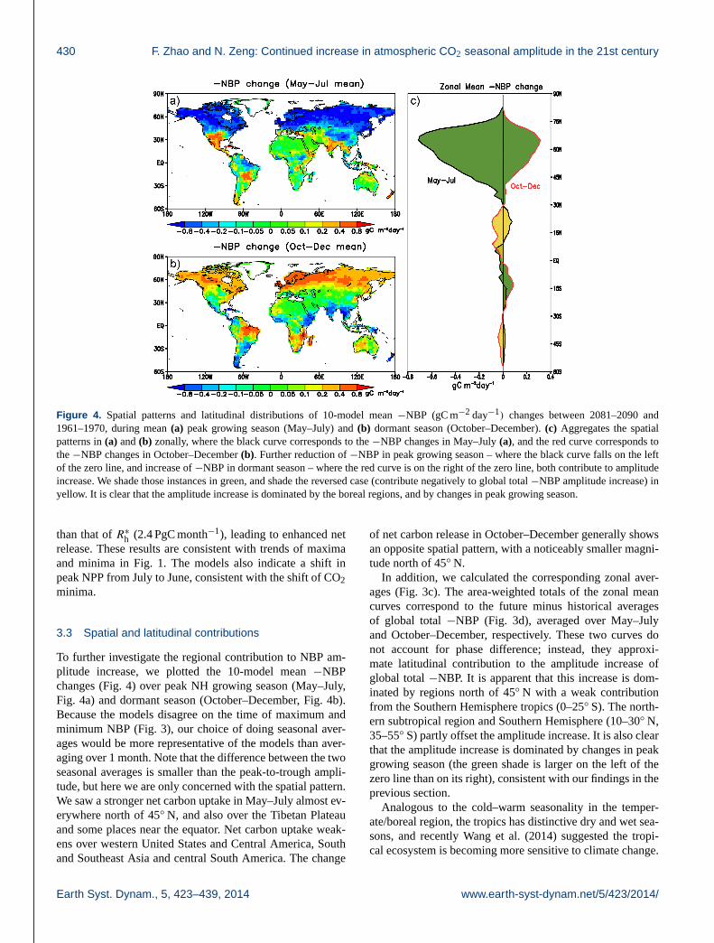
Figure 4. Spatial patterns and latitudinal distributions of 10-model mean −NBP (gC m−2 day−1) changes between 2081–2090 and

1961–1970, during mean (a) peak growing season (May–July) and (b) dormant season (October–December). (c) Aggregates the spatial

patterns in (a) and (b) zonally, where the black curve corresponds to the −NBP changes in May–July (a), and the red curve corresponds to

the −NBP changes in October–December (b). Further reduction of −NBP in peak growing season – where the black curve falls on the left

of the zero line, and increase of −NBP in dormant season – where the red curve is on the right of the zero line, both contribute to amplitude

increase. We shade those instances in green, and shade the reversed case (contribute negatively to global total −NBP amplitude increase) in

yellow. It is clear that the amplitude increase is dominated by the boreal regions, and by changes in peak growing season.

than that of R∗h (2.4 PgC month−1), leading to enhanced net

release. These results are consistent with trends of maxima

and minima in Fig. 1. The models also indicate a shift in

peak NPP from July to June, consistent with the shift of CO2

minima.

3.3 Spatial and latitudinal contributions

To further investigate the regional contribution to NBP am-

plitude increase, we plotted the 10-model mean −NBP

changes (Fig. 4) over peak NH growing season (May–July,

Fig. 4a) and dormant season (October–December, Fig. 4b).

Because the models disagree on the time of maximum and

minimum NBP (Fig. 3), our choice of doing seasonal aver-

ages would be more representative of the models than aver-

aging over 1 month. Note that the difference between the two

seasonal averages is smaller than the peak-to-trough ampli-

tude, but here we are only concerned with the spatial pattern.

We saw a stronger net carbon uptake in May–July almost ev-

erywhere north of 45◦ N, and also over the Tibetan Plateau

and some places near the equator. Net carbon uptake weak-

ens over western United States and Central America, South

and Southeast Asia and central South America. The change

of net carbon release in October–December generally shows

an opposite spatial pattern, with a noticeably smaller magni-

tude north of 45◦ N.

In addition, we calculated the corresponding zonal aver-

ages (Fig. 3c). The area-weighted totals of the zonal mean

curves correspond to the future minus historical averages

of global total −NBP (Fig. 3d), averaged over May–July

and October–December, respectively. These two curves do

not account for phase difference; instead, they approxi-

mate latitudinal contribution to the amplitude increase of

global total −NBP. It is apparent that this increase is dom-

inated by regions north of 45◦ N with a weak contribution

from the Southern Hemisphere tropics (0–25◦ S). The north-

ern subtropical region and Southern Hemisphere (10–30◦ N,

35–55◦ S) partly offset the amplitude increase. It is also clear

that the amplitude increase is dominated by changes in peak

growing season (the green shade is larger on the left of the

zero line than on its right), consistent with our findings in the

previous section.

Analogous to the cold–warm seasonality in the temper-

ate/boreal region, the tropics has distinctive dry and wet sea-

sons, and recently Wang et al. (2014) suggested the tropi-

cal ecosystem is becoming more sensitive to climate change.



In our analyses on the multi-model ensemble patterns, the

tropical region exhibits a small negative contribution to the

seasonal amplitude increase of global total −NBP. This does

not mean the net carbon flux in the tropics, which has a dif-

ferent seasonal cycle phase, would experience an amplitude

decrease in the future. To illustrate the seasonal amplitude

change at different latitudes, we show the zonal amplitude

of NBP in the historical (black) and future (red) periods for

all models (Fig. 5). At every 2◦ band, we first calculated

a 10-year mean seasonal cycle, then compute its amplitude

(maximum minus minimum). Most models predict an in-

crease in NBP seasonal amplitude at almost every latitude

under the RCP85 emission scenario. Only two of the mod-

els, CanESM2 and MIROC-ESM, predict decreased season-

ality for parts of the tropics and subtropics. Unlike in Fig. 4c,

an area-weighted integral cannot be performed due to differ-

ent phases zonally. The Southern Hemisphere has an oppo-

site phase from its northern counterpart, but its magnitude is

small due to its small land area. The two subtropical maxima

around 10◦ N and 10–15◦ S reflect the wet–dry seasonal shift

in the Intertropical Convergence Zone (ITCZ) and monsoon

movement. They are comparable to the NH maxima in terms

of both amplitude and amplitude increase for about a third of

the models, however they are out of phase and largely cancel

each other out.

To further illustrate this cancelation effect, we aggre-

gated monthly −NBP over six large regions: the globe

(90◦ S–90◦ N), northern boreal (50–90◦ N), northern temper-

ate (25–50◦ N), northern tropics (0–25◦ N), southern tropics

(25◦ S–0◦) and Southern Hemisphere (90–25◦ S; Fig. S1).

It is clear that the changes of global −NBP seasonal cy-

cle mostly come from the northern boreal region; it partly

comes from the northern temperature region in a few mod-

els. The seasonal cycle of the northern tropics is character-

ized by spring maxima and fall minima, and prominent in-

creases of its seasonal amplitude are found for BNU-ESM,

GFDL-ESM2M and IPSL-CM5A-LR. However, they are

largely counterbalanced by the southern tropics. For GFDL-

ESM2M, changes in the southern tropics are larger than

its northern counterpart, but even so, the net contribution

of tropical regions to its global −NBP seasonal amplitude

(September maxima minus June minima) increase is limited

to about 25 %, the largest of all models.

3.4 Mechanisms for amplitude increase

As discussed in Sect. 1, two major mechanisms for ampli-

tude increase identified in previous literature are CO2 fertil-

ization effect and high latitudes “greening” in a warmer cli-

mate. Both mechanisms lead to enhanced ecosystem produc-

tivity during peak growing season, and consequently more

biomass to decompose in dormant season, therefore increas-

ing the amplitude of NBP seasonal cycle. Because mod-

els have different climate and CO2 sensitivity (Arora et al.,

2013), their relative importance may vary. In the case of

Figure 5. Zonal amplitude of NBP from the 10 CMIP5 mod-

els (PgC month−1 per 2-degree band), averaged over 1961–1970

(black) and 2081–2090 (red). For each model, NBP is first regridded

to a 2× 2◦ common grid. Monthly zonal totals are then computed

for every 2-degree band, which determine the amplitude (maxi-

mum minus minimum) at every band. The Southern Hemisphere

has an opposite phase from its northern counterpart, but its magni-

tude is small due to its small land area. The two subtropical maxima

around 10◦ N and 10–15◦ S reflect the wet–dry seasonal shift in the

Intertropical Convergence Zone (ITCZ) and monsoon movement.

They have similar magnitude as the Northern Hemisphere maxima

in about a third of the models, however their net contribution to

global total NBP seasonal amplitude is small, because they are out

of phase and largely cancel each other out.



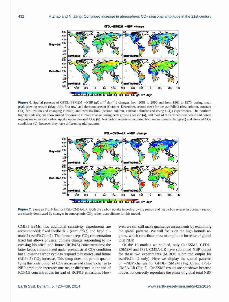
Figure 6. Spatial patterns of GFDL-ESM2M −NBP (gC m−2 day−1) changes from 2081 to 2090 and from 1961 to 1970, during mean

peak growing season (May–July, first row) and dormant season (October–December, second row) for the esmFdbk2 (first column, constant

CO2 fertilization and changing climate) and esmFixClim2 (second column, constant climate and rising CO2) experiments. The northern

high latitude regions show mixed response to climate change during peak growing season (a), and most of the northern temperate and boreal

regions see enhanced carbon uptake under elevated CO2 (b). Net carbon release is increased both under climate change (c) and elevated CO2

conditions (d), however they have different spatial patterns.

Figure 7. Same as Fig. 6, but for IPSL-CM5A-LR. Both the carbon uptake in peak growing season and net carbon release in dormant season

are clearly dominated by changes in atmospheric CO2 rather than climate for this model.

CMIP5 ESMs, two additional sensitivity experiments are

recommended: fixed feedback 2 (esmFdbk2) and fixed cli-

mate 2 (esmFixClim2). The former keeps CO2 concentration

fixed but allows physical climate change responding to in-

creasing historical and future (RCP4.5) concentrations; the

latter keeps climate fixed under preindustrial CO2 condition

but allows the carbon cycle to respond to historical and future

(RCP4.5) CO2 increase. This setup does not permit quanti-

fying the contribution of CO2 increase and climate change to

NBP amplitude increase: one major difference is the use of

RCP4.5 concentrations instead of RCP8.5 emissions. How-

ever, we can still make qualitative assessments by examining

the spatial patterns. We will focus on the high latitude re-

gions, which contribute most to amplitude increase of global

total NBP.

Of the 10 models we studied, only CanESM2, GFDL-

ESM2M and IPSL-CM5A-LR have submitted NBP output

for these two experiments (MIROC submitted output for

esmFixClim2 only). Here we display the spatial patterns

of −NBP changes for GFDL-ESM2M (Fig. 6) and IPSL-

CM5A-LR (Fig. 7). CanESM2 results are not shown because

it does not correctly reproduce the phase of global total NBP



seasonal cycle. The changes of −NBP for both models dur-

ing peak growing season are clearly dominated by CO2 fer-

tilization effect (right panels). In contrast, climate change

under fixed CO2 fertilization conditions has mixed effects

on high latitude regions. Northern high latitude net carbon

release in October–December is increased both under cli-

mate change (Fig. 6c) and elevated CO2 conditions (Fig. 6d)

for GFDL-ESM2M, but over different regions. For IPSL-

CM5A-LR however, net carbon release increase in regions

north of 45◦ N is only obvious under elevated CO2 condition.

Our results only indicate CO2 fertilization effect is the

dominant factor for NBP seasonal amplitude increase in

some models. For models with strong carbon-climate feed-

backs and weak/moderate water constraints in northern high

latitude regions, climate change may be more important.

However, we cannot find a clear example due to data

availability. MIROC-ESM is known to have strong carbon-

climate feedback (Arora et al., 2013). From its simulation

under fixed climate (figure not shown), we found no obvious

patterns of widespread net carbon release increase in dor-

mant season, suggesting climate change may play a bigger

role for this model. The HadGEM model is another possible

candidate; it is also a particularly interesting model to an-

alyze since one of its historical simulations represented the

largest increase in CO2 amplitude in Graven et al. (2013).

Unfortunately, for the ESM simulations, both CO2 and NBP

from HadGEM are not available on the ESGF servers.

3.5 Relationship with mean carbon sink

Our analyses above suggest CO2 fertilization effect is a ma-

jor mechanism causing the amplitude increase in some mod-

els. If it is important in most models, we expect to see mod-

els with a larger change in mean carbon sink simulate a

higher increase in seasonal amplitude. By plotting the−NBP

change against NBP seasonal amplitude increase for all 10

models (Fig. 8), we found there is indeed a negative cross-

model correlation (R =−0.73, p < 0.05), indicating mod-

els with a stronger net carbon uptake are likely to simulate

a larger increase in NBP seasonal amplitude. Note that this

result is based on the 10 models we analyzed; it is subject

to large uncertainty and may change substantially with in-

clusion or exclusion of certain model(s). Again all models

show an increase in NBP seasonal amplitude, even though

they disagree on the direction of future NBP change. While

our study hint at a possible relationship between mean car-

bon sink and NBP seasonal amplitude, it is beyond our scope

to discuss further, or comment on why models show such

different mean sink estimate. Interested readers may refer

to the insightful discussion on this issue in Friedlingstein et

al. (2013).

Figure 8. Relationship between −NBP change and increase of

NBP seasonal amplitude, calculated as the differences between

2081–2090 and 1961–1970 for 10 CMIP5 ESMs. The negative

cross-model correlation (R =−0.73, p < 0.05) suggests that a

model with a larger net carbon sink increase is likely to simulate

a higher increase in NBP seasonal amplitude.

4 Discussions

We have primarily focused on model ensembles of aggre-

gated quantities. Ensemble patterns are sometimes domi-

nated by only a few models due to large seasonality vari-

ations among the models. However, the close examination

of each individual model show that the spatial patterns of

−NBP change during peak growing season (May–July) are

all dominated by high latitude regions (approximately north

of 45◦ N). In CESM1-BGC and NorESM1-ME models, en-

hanced net carbon uptake are confined to some of the high

latitude regions (Fig. S2 in the Supplement). Models dif-

fer on finer details. For example, about half of the models

predict an obvious increase of net carbon uptake for the Ti-

betan Plateau. It is worth mentioning that the esmFixClim2

experiment of MIROC-ESM shows little change in NBP for

this region under elevated CO2 alone. High latitude regions

also dominate the increase of net carbon release in Octo-

ber–December for most models (Fig. S3). One exception is

INM-CM4, which displays very small change in the dormant

season, and most of its NBP amplitude increase comes from

enhanced carbon uptake during peak growing season. BNU-

ESM and CanESM2 have some limitations in reproducing

the correct phase of global −NBP seasonal cycle. Exclu-

sion of these two models from ensemble mean calculation

exhibits very similar spatial and zonal patterns as shown in

Fig. 4. Another caveat is the assumption of 1961–1970 as the

historical condition and 2081–2090 as future condition. This

choice is valid if the selected variables have roughly mono-

tonic trends, and 10 years is long enough to smooth out most

of the interannual variability. Figure 2 suggests that this as-



Figure 9. CO2 mean seasonal amplitude (ppm) during 2001–2005

and increase in CO2 seasonal amplitude at Mauna Loa during

1959–2005 (% yr−1, linear trend) from eight CMIP5 models and

observation. The big black circle represent surface CO2 observa-

tion at Mauna Loa, Hawaii (19.5◦ N, 155.6◦W; 3400 m above sea

level). The colored squares represent the 700 hPa (close to the alti-

tude of Mauna Loa station surface) CO2 output at the original grid

that covers Mauna Loa from each of the eight models. Error bars

indicate±1 standard error in the trend calculation. Compared to the

surface observation, only MPI-ESM-LR and GFDL-ESM2M over-

estimate CO2 mean seasonal amplitude at Mauna Loa, while the

other models underestimate this amplitude. Models split between

overestimating and underestimating the CO2 seasonal amplitude in-

crease at Mauna Loa.

sumption is quite reasonable for model ensembles, and ac-

ceptable for individual models.

We presented aggregated quantities due to large model un-

certainty in space. We have largely omitted model evalua-

tion against observations (due to limited observation during

1961–1970). However, this step can be helpful in model eval-

uation studies (Anav et al., 2013; Peng et al., 2014). One

concern is to examine whether the models can reproduce

observed CO2 seasonal amplitude increase at the two sta-

tions with longest observation records – Mauna Loa, Hawaii

and Point Barrow, Alaska. To address this issue, we ex-

tracted simulated CO2 concentration from eight models at

their model grid that is closest to Mauna Loa in the three-

dimensional space (similar procedure for Point Barrow). The

results of this comparison at one model grid can reflect mul-

tiple sources of model uncertainties (such as uncertainties

in the atmospheric tracer transport and mixing simulations).

For example, GFDL-ESM2M is known to simulate a damped

CO2 gradient (Dunne et al., 2013) which has long been iden-

tified as a deficit in models of the atmospheric CO2 cycle

(Fung et al., 1987).

Figure 9 (and Fig. S4 for more details) presents the

changes of CO2 seasonal amplitude at Mauna Loa for the

Figure 10. CO2 mean seasonal amplitude (ppm) during 2001–2005

and increase in CO2 seasonal amplitude at Pt. Barrow during

1974–2005 (% yr−1, linear trend) from eight CMIP5 ESMs and ob-

servation. The big black circle represent surface CO2 observation

at Point Barrow, Alaska (71.3◦ N, 156.5◦W; 11 m above sea level).

The colored squares represent the CO2 output at lowest model level

(four models at 1000 hPa, and four at 925 hPa) at the original grid

that covers Point Barrow from each of the eight models. Error bars

indicate ±1 standard error in the trend calculation. Compared to

the surface observation, only MPI-ESM-LR overestimate the CO2

mean seasonal amplitude at Point Barrow, while the other models

underestimate this amplitude. Models split between overestimating

and underestimating the CO2 seasonal amplitude increase at Point

Barrow.

models and observation. CO2 seasonal amplitude is under-

estimated by a factor of 2 in three-quarters of the models.

However, the amplitude increase from ensemble model es-

timate (0.36± 0.24 % yr−1, error range represents one stan-

dard deviation model spread) is much closer to observation

(0.34±0.07 % yr−1, error range represents one standard error

of the least-squared trend calculation). MPI-ESM-LR repro-

duces both the magnitude and trend of Mauna Loa CO2 sea-

sonal amplitude reasonably well. For Point Barrow (Figs. 10

and S5), MPI-ESM-LR also simulates a similar amplitude

increase to observation, but the magnitude of amplitude is

much larger (almost twice). All other models underestimate

the amplitude, but for the amplitude increase, the model en-

semble (0.46± 0.21 % yr−1) again is similar to observation

(0.43±0.10 % yr−1). MRI-ESM1 is found to reproduce both

the magnitude and increase of Point Barrow CO2 amplitude

quite well.

Graven et al. (2013) found the CMIP5 models substan-

tially underestimate the amplitude increase of CO2 north of

45◦ N at altitude of 3 to 6 km. However, we did not find

that the models underestimate Point Barrow CO2 amplitude

increase at surface level. One big difference is the obser-

vational data used for comparison. During the 1974–2005



Figure 11. Changes of tree cover fractions between future (2081–2090) and historical (1961–1970) periods from six CMIP5 ESMs. The

values represent fractional cover changes relative to the whole grid cell, instead of relative change of tree cover. For MPI-ESM-LR and

INM-CM4, tree fraction has increased over wide areas of the northern high latitude regions. For MIROC-ESM, tree fraction has generally

decreased over the same regions, possibly in response to a hotter and drier climate condition.

period, CO2 seasonal amplitude increases by 0.43 % yr−1,

or 21.5 % over 50 years at the Point Barrow station. This

is much lower than the ∼ 50 % amplitude increase found

between the two aircraft campaigns during 1958–1961 and

2009–2011 (Graven et al., 2013). This difference might be

attributed to mechanisms controlling the vertical profile of

CO2 concentration. It is also not clear to what extent the large

interannual variability of CO2 seasonal amplitude affects the

trend estimation of observed CO2 amplitude increase.

Under the RCP8.5 emission scenario, CMIP5 showed a

62± 19 % increase of CO2 seasonal cycle globally from

1961–1970 to 2081–2090. The increase is 85± 48 % at

Mauna Loa (range indicates one standard deviation model

spread), and 110± 42 % at Point Barrow. Even though the

CMIP5 models are able to reproduce the increase of CO2

seasonal amplitude at the two locations, some of the models

rely heavily on the CO2 fertilization mechanism, which may

be too strong compared to observational evidence. Previous

research suggest it should explain no more than 25 % of the

observation at a high fertilization effect permitted by lab ex-

periments (Kohlmaier et al., 1989). Similarly, Randerson et

al. (1997) found the linear factor of CO2 fertilization has to

be 4 to 6 times greater than the mean of the experimental val-

ues, in order to explain the 0.66 % yr−1 amplitude increase

(north of 55◦ N) during 1981–1995. Recent studies have in-

dicated that some important mechanisms, such as changes in

ecosystem structure and distribution (Graven et al., 2013) and

land use intensification (Zeng et al., 2014), are missing in the

current CMIP5 models. Yet another main source of uncer-

tainty is future CO2 emissions. The RCP8.5 scenario used to

drive the ESMs is on the high side of future scenarios. Also,

the emission-driven runs simulate higher CO2 than observed

over the historical period, and such biases are likely to accu-

mulate over time as the increase of atmospheric CO2 growth

rate accelerates (Hoffman et al., 2014).

The models do not have the same strength of carbon-

climate feedback, but even if they do, their response to cli-

mate change may vary significantly simply because they sim-

ulate very different climate change. To briefly address this

issue, we present soil moisture (Figs. S6 and S7) and near-

surface temperature (Figs. S8 and S9) changes for all models.

All the models show temperature increase, but in different

ranges. The more prominent difference was observed in the

spatial pattern of soil moisture changes predicted by models.

The combined effect of soil moisture regimes, temperature

change and plant functional type (PFT) specifications could

cause diverse behaviors of models over same regions. Such



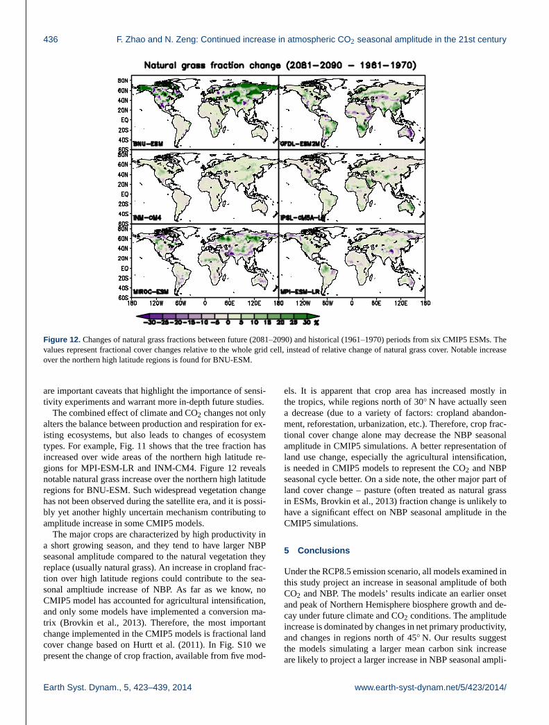
Figure 12. Changes of natural grass fractions between future (2081–2090) and historical (1961–1970) periods from six CMIP5 ESMs. The

values represent fractional cover changes relative to the whole grid cell, instead of relative change of natural grass cover. Notable increase

over the northern high latitude regions is found for BNU-ESM.

are important caveats that highlight the importance of sensi-

tivity experiments and warrant more in-depth future studies.

The combined effect of climate and CO2 changes not only

alters the balance between production and respiration for ex-

isting ecosystems, but also leads to changes of ecosystem

types. For example, Fig. 11 shows that the tree fraction has

increased over wide areas of the northern high latitude re-

gions for MPI-ESM-LR and INM-CM4. Figure 12 reveals

notable natural grass increase over the northern high latitude

regions for BNU-ESM. Such widespread vegetation change

has not been observed during the satellite era, and it is possi-

bly yet another highly uncertain mechanism contributing to

amplitude increase in some CMIP5 models.

The major crops are characterized by high productivity in

a short growing season, and they tend to have larger NBP

seasonal amplitude compared to the natural vegetation they

replace (usually natural grass). An increase in cropland frac-

tion over high latitude regions could contribute to the sea-

sonal ampltiude increase of NBP. As far as we know, no

CMIP5 model has accounted for agricultural intensification,

and only some models have implemented a conversion ma-

trix (Brovkin et al., 2013). Therefore, the most important

change implemented in the CMIP5 models is fractional land

cover change based on Hurtt et al. (2011). In Fig. S10 we

present the change of crop fraction, available from five mod-

els. It is apparent that crop area has increased mostly in

the tropics, while regions north of 30◦ N have actually seen

a decrease (due to a variety of factors: cropland abandon-

ment, reforestation, urbanization, etc.). Therefore, crop frac-

tional cover change alone may decrease the NBP seasonal

amplitude in CMIP5 simulations. A better representation of

land use change, especially the agricultural intensification,

is needed in CMIP5 models to represent the CO2 and NBP

seasonal cycle better. On a side note, the other major part of

land cover change – pasture (often treated as natural grass

in ESMs, Brovkin et al., 2013) fraction change is unlikely to

have a significant effect on NBP seasonal amplitude in the

CMIP5 simulations.

5 Conclusions

Under the RCP8.5 emission scenario, all models examined in

this study project an increase in seasonal amplitude of both

CO2 and NBP. The models’ results indicate an earlier onset

and peak of Northern Hemisphere biosphere growth and de-

cay under future climate and CO2 conditions. The amplitude

increase is dominated by changes in net primary productivity,

and changes in regions north of 45◦ N. Our results suggest

the models simulating a larger mean carbon sink increase

are likely to project a larger increase in NBP seasonal ampli-



tude. Considerable model spread is found, likely due to dif-

ferent model setup and complexity, different climate condi-

tions simulated by the models, sensitivity to CO2 and climate

and their combined effects, and strength of feedbacks. Our

findings indicate factors including enhanced CO2 fertiliza-

tion and lengthening of growing season in high-latitude re-

gions outcompetes possible severe drought and forest degra-

dation (leading to loss of biosphere productivity) in the fu-

ture.

Despite of the model consensus in global CO2 and NBP

seasonal amplitude increase, and a reasonable representa-

tion of CO2 seasonal amplitude increase at Mauna Loa

and Point Barrow compared to surface in situ observations,

the mechanisms contributing to these changes are debat-

able. CO2 fertilization may be too strong, and factors like

ecosystem change and agricultural intensification are under-

represented or missing in the CMIP5 ESMs. Future model-

intercomparison projects should encourage models to par-

ticipate in consistent and comprehensive sensitivity experi-

ments.

The Supplement related to this article is available online

at doi:10.5194/esd-5-423-2014-supplement.

Acknowledgements. We acknowledge the World Climate

Research Programme’s Working Group on Coupled Modeling,

which is responsible for CMIP, and we thank the climate modeling

groups (listed in Table 1) for producing and making available their

model output. For CMIP the US Department of Energy’s Program

for Climate Model Diagnosis and Intercomparison provides coor-

dinating support and led development of software infrastructure in

partnership with the Global Organization for Earth System Science

Portals. The authors also thank NOAA for providing global mean

CO2 estimates, and Yutong Pan for processing part of CMIP5

model data. We are grateful to the two anonymous reviewers

for their helpful comments and suggestions. This research was

supported by NOAA (NA10OAR4310248 and NA09NES4400006)

and NSF (AGS-1129088).

Edited by: J. Canadell

References

Anav, A., Friedlingstein, P., Kidston, M., Bopp, L., Ciais, P., Cox,

P., Jones, C., Jung, M., Myneni, R., and Zhu, Z.: Evaluating

the Land and Ocean Components of the Global Carbon Cycle

in the CMIP5 Earth System Models, J. Clim., 26, 6801–6843,

doi:10.1175/JCLI-D-12-00417.1, 2013.

Andres, R. J., Gregg, J. S., Losey, L., Marland, G., and Boden,

T. A.: Monthly, global emissions of carbon dioxide from fos-

sil fuel consumption, Tellus B, 63, 309–327, doi:10.1111/j.1600-

0889.2011.00530.x, 2011.

Arora, V. K., Scinocca, J. F., Boer, G. J., Christian, J. R., Denman,

K. L., Flato, G. M., Kharin, V. V., Lee, W. G., and Merryfield, W.

J.: Carbon emission limits required to satisfy future representa-

tive concentration pathways of greenhouse gases, Geophys. Res.

Lett., 38, L05805, doi:10.1029/2010GL046270, 2011.

Arora, V. K., Boer, G. J., Friedlingstein, P., Eby, M., Jones, C.

D., Christian, J. R., Bonan, G., Bopp, L., Brovkin, V., Cad-

ule, P., Hajima, T., Ilyina, T., Lindsay, K., Tjiputra, J. F., and

Wu, T.: Carbon–Concentration and Carbon–Climate Feedbacks

in CMIP5 Earth System Models, J. Clim., 26, 5289–5314,

doi:10.1175/JCLI-D-12-00494.1, 2013.

Bacastow, R. B., Keeling, C. D., and Whorf, T. P.: Seasonal am-

plitude increase in atmospheric CO2 concetration at Mauna

Loa, Hawaii, 1959–1982, J. Geophys. Res., 90, 10529–10540,

doi:10.1029/JD090iD06p10529, 1985.

Brovkin, V., Boysen, L., Arora, V. K., Boisier, J. P., Cadule, P.,

Chini, L., Claussen, M., Friedlingstein, P., Gayler, V., van den

Hurk, B. J. J. M., Hurtt, G. C., Jones, C. D., Kato, E., de Noblet-

Ducoudré, N., Pacifico, F., Pongratz, J., and Weiss, M.: Effect of

Anthropogenic Land-Use and Land-Cover Changes on Climate

and Land Carbon Storage in CMIP5 Projections for the Twenty-

First Century, J. Clim., 26, 6859–6881, doi:10.1175/JCLI-D-12-

00623.1, 2013.

Buermann, W., Lintner, B. R., Koven, C. D., Angert, A., Pinzon,

J. E., Tucker, C. J., and Fung, I. Y.: The changing carbon cy-

cle at Mauna Loa Observatory, Proc. Natl. Acad. Sci. USA, 104,

4249–4254, 2007.

Cleveland, W., Freeny, A. E., and Graedel, T. E.: The Seasonal

Component of Atmospheric CO2: Information From New Ap-

proaches to the Decomposition of Seasonal Time Series, J. Geo-

phys. Res., 88, 10934–10946, 1983.

Conway, T. J., Tans, P. P., Waterman, L. S., Thoning, K. W., Kitzis,

D. R., Masarie, K. A., and Zhang, N.: Evidence for interannual

variability of the carbon cycle from the National Oceanic and At-

mospheric Administration / Climate Monitoring and Diagnostics

Laboratory Global Air Sampling Network, J. Geophys. Res., 99,

22831–22855, 1994.

Dufresne, J.-L., Foujols, M.-A., Denvil, S., Caubel, A., Marti, O.,

Aumont, O., Balkanski, Y., Bekki, S., Bellenger, H., Benshila,

R., Bony, S., Bopp, L., Braconnot, P., Brockmann, P., Cadule, P.,

Cheruy, F., Codron, F., Cozic, A., Cugnet, D., Noblet, N., Duvel,

J.-P., Ethé, C., Fairhead, L., Fichefet, T., Flavoni, S., Friedling-

stein, P., Grandpeix, J.-Y., Guez, L., Guilyardi, E., Hauglus-

taine, D., Hourdin, F., Idelkadi, A., Ghattas, J., Joussaume, S.,

Kageyama, M., Krinner, G., Labetoulle, S., Lahellec, A., Lefeb-

vre, M.-P., Lefevre, F., Levy, C., Li, Z. X., Lloyd, J., Lott, F.,

Madec, G., Mancip, M., Marchand, M., Masson, S., Meurdes-

oif, Y., Mignot, J., Musat, I., Parouty, S., Polcher, J., Rio, C.,

Schulz, M., Swingedouw, D., Szopa, S., Talandier, C., Terray, P.,

and Viovy, N.: Climate change projections using the IPSL-CM5

Earth System Model: from CMIP3 to CMIP5, Clim. Dyn., 40,

2123–2165, doi:10.1007/s00382-012-1636-1, 2013.

Dunne, J. P., John, J. G., Shevliakova, E., Stouffer, R. J., Krasting,

J. P., Malyshev, S. L., Milly, P. C. D., Sentman, L. T., Adcroft,

A. J., Cooke, W., Dunne, K. A., Griffies, S. M., Hallberg, R.

W., Harrison, M. J., Levy, H., Wittenberg, A. T., Phillips, P. J.,

and Zadeh, N.: GFDL’s ESM2 Global Coupled Climate–Carbon

Earth System Models. Part II: Carbon System Formulation and


http://dx.doi.org/10.5194/esd-5-423-2014-supplement

http://dx.doi.org/10.1175/JCLI-D-12-00417.1

http://dx.doi.org/10.1111/j.1600-0889.2011.00530.x

http://dx.doi.org/10.1111/j.1600-0889.2011.00530.x

http://dx.doi.org/10.1029/2010GL046270


http://dx.doi.org/10.1029/JD090iD06p10529



http://dx.doi.org/10.1007/s00382-012-1636-1


Baseline Simulation Characteristics, J. Clim., 26, 2247–2267,

doi:10.1175/JCLI-D-12-00150.1, 2013.

Friedlingstein, P., Meinshausen, M., Arora, V. K., Jones, C. D.,

Anav, A., Liddicoat, S. K., and Knutti, R.: Uncertainties in

CMIP5 climate projections due to carbon cycle feedbacks, J.

Clim., 27, 511–526, doi:10.1175/JCLI-D-12-00579.1, 2013.

Fung, I. Y., Tucker, C. J., and Prentice, K. C.: Application of Ad-

vanced Very High Resolution Radiometer vegetation index to

study atmosphere-biosphere exchange of CO2, J. Geophys. Res.,

92, 2999–3015, doi:10.1029/JD092iD03p02999, 1987.

Graven, H. D., Keeling, R. F., Piper, S. C., Patra, P. K., Stephens,

B. B., Wofsy, S. C., Welp, L. R., Sweeney, C., Tans, P.

P., Kelley, J. J., Daube, B. C., Kort, E. a, Santoni, G. W.,

and Bent, J. D.: Enhanced Seasonal Exchange of CO2 by

Northern Ecosystems Since 1960, Science, 341, 1085–1089,

doi:10.1126/science.1239207, 2013.

Gurney, K. R. and Eckels, W. J.: Regional trends in terrestrial

carbon exchange and their seasonal signatures, Tellus B, 63,

328–339, doi:10.1111/j.1600-0889.2011.00534.x, 2011.

Hall, C. A. S., Ekdahl, C. A., and Wartenberg, D. E.: A fifteen-year

record of biotic metabolism in the Northern Hemisphere, Nature,

255, 136–138, doi:10.1038/255136a0, 1975.

Hoffman, F. M., Randerson, J. T., Arora, V. K., Bao, Q., Cad-

ule, P., Ji, D., Jones, C. D., Kawamiya, M., Khatiwala, S.,

Lindsay, K., Obata, A., Shevliakova, E., Six, K. D., Tjipu-

tra, J. F., Volodin, E. M., and Wu, T.: Causes and implica-

tions of persistent atmospheric carbon dioxide biases in Earth

System Models, J. Geophys. Res.-Biogeosci., 119, 141–162,

doi:10.1002/2013JG002381, 2014.

Hurtt, G. C., Chini, L. P., Frolking, S., Betts, R. a, Feddema, J.,

Fischer, G., Fisk, J. P., Hibbard, K., Houghton, R. a, Janetos,

a, Jones, C. D., Kindermann, G., Kinoshita, T., Klein Gold-

ewijk, K., Riahi, K., Shevliakova, E., Smith, S., Stehfest, E.,

Thomson, a, Thornton, P., Van Vuuren, D. P., and Wang, Y.

P.: Harmonization of land-use scenarios for the period 1500-

2100: 600 years of global gridded annual land-use transitions,

wood harvest, and resulting secondary lands, Clim. Change, 109,

117–161, doi:10.1007/s10584-011-0153-2, 2011.

Ilyina, T., Six, K. D., Segschneider, J., Maier-reimer, E., Li, H.,

and Núñez-Riboni, I.: Global ocean biogeochemistry model

HAMOCC?: Model architecture and performance as component

of the MPI-Earth system model in different CMIP5 experimental

realizations, J. Adv. Model. Earth Syst., 5, 287–315, 2013.

International Panel on Climate Change (IPCC): Climate Change

2013: the Physical Science Basis. Working Group 1 Contribution

to the Fifth Assessment Report of the International Panel on Cli-

mate Change International Panel on Climate Change, Cambridge

University Press, Cambridge, New York., 2013.

Ji, D., Wang, L., Feng, J., Wu, Q., Cheng, H., Zhang, Q., Yang,

J., Dong, W., Dai, Y., Gong, D., Zhang, R.-H., Wang, X., Liu,

J., Moore, J. C., Chen, D., and Zhou, M.: Description and

basic evaluation of Beijing Normal University Earth System

Model (BNU-ESM) version 1, Geosci. Model Dev., 7, 2039-

2064, doi:10.5194/gmd-7-2039-2014, 2014.

Kaminski, T., Giering, R., and Heimann, M.: Sensitivity of the

seasonal cycle of CO2 at remote monitoring stations with re-

spect to seasonal surface exchange fluxes determined with the

adjoint of an atmospheric transport model, Phys. Chem. Earth,

21, 457–462, 1996.

Keeling, C. D., Whorf, T. P., Wahlen, M., and van der Plichtt, J.: In-

terannual extremes in the rate of rise of atmospheric carbon diox-

ide since 1980, Nature, 375, 666–670, doi:10.1038/375666a0,

1995.

Keeling, C. D., Chin, J. F. S., and Whorf, T. P.: Increased activity

of northern vegetation inferred from atmospheric CO2 measure-

ments, Nature, 382, 146–149, doi:10.1038/382146a0, 1996.

Kohlmaier, G. H., Siré, E. O., Janecek, A., Keeling, C. D., Piper, S.

C., and Revelle, R.: Modelling the seasonal contribution of a CO2

fertilization effect of the terrestrial vegetation to the amplitude

increase in atmospheric CO2 at Mauna Loa Observatory, Tellus

B, 41, 487–510, doi:10.1111/j.1600-0889.1989.tb00137.x, 1989.

Long, M. C., Lindsay, K., Peacock, S., Moore, J. K., and Doney,

S. C.: Twentieth-Century Oceanic Carbon Uptake and Storage in

CESM1(BGC), J. Clim., 26, 6775–6800, doi:10.1175/JCLI-D-

12-00184.1, 2013.

McGuire, A. D., Sitch, S., Clein, J. S., Dargaville, R., Esser, G.,

Foley, J., Heimann, M., Joos, F., Kaplan, J., Kicklighter, D. W.,

Meier, R. a, Melillo, J. M., Moore III, B., Prentice, I. C., Ra-

mankutty, N., Reichenau, T., Schloss, A., Tian, H., Williams, L.

J., and Wittenberg, U.: Carbon balance of the terrestrial biosphere

in the twentieth century: Analyses of CO2, climate and land use

effects with four process-based ecosystem models, Global Bio-

geochem. Cy., 15, 183–206, 2001.

Moss, R. H., Edmonds, J. a, Hibbard, K. a, Manning, M. R., Rose,

S. K., van Vuuren, D. P., Carter, T. R., Emori, S., Kainuma, M.,

Kram, T., Meehl, G. a, Mitchell, J. F. B., Nakicenovic, N., Ri-

ahi, K., Smith, S. J., Stouffer, R. J., Thomson, A. M., Weyant,

J. P., and Wilbanks, T. J.: The next generation of scenarios for

climate change research and assessment, Nature, 463, 747–756,

doi:10.1038/nature08823, 2010.

Pearman, G. I. and Hyson, P.: The annual variation of atmospheric

CO2 concentration Observed in the Northern Hemisphere, J.

Geophys. Res., 86, 9839–9843, 1981.

Peng, S., Ciais, P., Chevalier, F., Peylin, P., Cadule, P., Sitch, S.,

Piao, S., Ahlström, A., Huntingford, C., Levy, P., Li, X., Liu, Y.,

Lomas, M., Poulter, B., Viovy, N., Wang, T., Wang, X., Zaehle,

S., Zeng, N., Zhao, F. and Zhao, H.: Benchmarking the seasonal

cycle of CO2 fluxes simulated by terrestrial ecosystem models,

Global Biogeochem. Cy., in review, 2014.

Peylin, P., Law, R. M., Gurney, K. R., Chevallier, F., Jacobson,

A. R., Maki, T., Niwa, Y., Patra, P. K., Peters, W., Rayner, P.

J., Rödenbeck, C., van der Laan-Luijkx, I. T., and Zhang, X.:

Global atmospheric carbon budget: results from an ensemble of

atmospheric CO2 inversions, Biogeosciences, 10, 6699–6720,

doi:10.5194/bg-10-6699-2013, 2013.

Piao, S., Sitch, S., Ciais, P., Friedlingstein, P., Peylin, P., Wang, X.,

Ahlström, A., Anav, A., Canadell, J. G., Cong, N., Huntingford,

C., Jung, M., Levis, S., Levy, P. E., Li, J., Lin, X., Lomas, M.

R., Lu, M., Luo, Y., Ma, Y., Myneni, R. B., Poulter, B., Sun,

Z., Wang, T., Viovy, N., Zaehle, S., and Zeng, N.: Evaluation of

terrestrial carbon cycle models for their response to climate vari-

ability and to CO2 trends, Glob. Chang. Biol., 19, 2117–2132,

doi:10.1111/gcb.12187, 2013.

Randerson, J. T., Thompson, M. V, Conway, T. J., Fung, I. Y.,

Field, C. B., Randerson, T., Thompson, V., Conway, J., and Field,

B.: The contribution of terrestrial sources and sinks to trends in

the seasonal cycle of atmospheric carbon dioxide, Global Bio-

geochem. Cy., 11, 535–560, doi:10.1029/97gb02268, 1997.





http://dx.doi.org/10.1126/science.1239207

http://dx.doi.org/10.1111/j.1600-0889.2011.00534.x

http://dx.doi.org/10.1038/255136a0

http://dx.doi.org/10.1002/2013JG002381

http://dx.doi.org/10.1007/s10584-011-0153-2

http://dx.doi.org/10.5194/gmd-7-2039-2014

http://dx.doi.org/10.1038/375666a0

http://dx.doi.org/10.1038/382146a0

http://dx.doi.org/10.1111/j.1600-0889.1989.tb00137.x



http://dx.doi.org/10.1038/nature08823

http://dx.doi.org/10.5194/bg-10-6699-2013

http://dx.doi.org/10.1111/gcb.12187

http://dx.doi.org/10.1029/97gb02268


Randerson, J. T., Field, C. B., Fung, I. Y., and Tans, P.

P.: Increases in early season ecosystem uptake explain re-

cent changes in the seasonal cycle of atmospheric CO2 at

high northern latitudes, Geophys. Res. Lett., 26, 2765–2768,

doi:10.1029/1999GL900500, 1999.

Reiners, W.: Terrestrial detritus and the carbon cycle, in: US AEC

Conf. 720510, 317–327., 1973.

Taylor, K. E., Stouffer, R. J., and Meehl, G. a.: An Overview of

CMIP5 and the Experiment Design, B. Am. Meteorol. Soc., 93,

485–498, doi:10.1175/BAMS-D-11-00094.1, 2012.

Thoning, K. W., Tans, P. P., and Komhyr, W. D.: Atmospheric

carbon dioxide at Mauna Loa Observatory: 2, Analysis of the

NOAA GMCC data, 1974–1985, J. Geophys. Res., 94, 8549,

doi:10.1029/JD094iD06p08549, 1989.

Tjiputra, J. F., Roelandt, C., Bentsen, M., Lawrence, D. M.,

Lorentzen, T., Schwinger, J., Seland, Ø., and Heinze, C.: Eval-

uation of the carbon cycle components in the Norwegian Earth

System Model (NorESM), Geosci. Model Dev., 6, 301–325,

doi:10.5194/gmd-6-301-2013, 2013.

Volodin, E. M., Dianskii, N. A., and Gusev, A. V.: Simulating

present-day climate with the INMCM4.0 coupled model of the

atmospheric and oceanic general circulations, Izv. Atmos. Ocean.

Phys., 46, 414–431, doi:10.1134/S000143381004002X, 2010.

Wang, X., Piao, S., Ciais, P., Friedlingstein, P., Myneni, R. B.,

Cox, P., Heimann, M., Miller, J., Peng, S., Wang, T., Yang,

H., and Chen, A.: A two-fold increase of carbon cycle sensi-

tivity to tropical temperature variations., Nature, 506, 212–215,

doi:10.1038/nature12915, 2014.

Watanabe, S., Hajima, T., Sudo, K., Nagashima, T., Takemura, T.,

Okajima, H., Nozawa, T., Kawase, H., Abe, M., Yokohata, T.,

Ise, T., Sato, H., Kato, E., Takata, K., Emori, S., and Kawamiya,

M.: MIROC-ESM 2010: model description and basic results of

CMIP5-20c3m experiments, Geosci. Model Dev., 4, 845–872,

doi:10.5194/gmd-4-845-2011, 2011.

Whittaker, R. H. and Likens, G. E.: Primary produc-

tion: The biosphere and man, Hum. Ecol., 1, 357–369,

doi:10.1007/BF01536732, 1973.

Williams, D. N., Taylor, K. E., Cinquini, L., Evans, B., Kawamiya,

M., Lawrence, B. N., and Middleton, D. E.: The Earth System

Grid Federation?: Software Framework Supporting CMIP5 Data

Analysis and Dissemination, CLIVAR Exch., 16, 40–42, 2011.

Yukimoto, S., Yoshimura, H., Hosaka, M., Sakami, T., Tsujino, H.,

Hirabara, M., Tanaka, T. Y., Deushi, M., Obata, A., Nakano, H.,

Adachi, Y., Shindo, E., Yabu, S., Ose, T., and Kitoh, A.: Meteoro-

logical Research Institute-Earth System Model Version 1 (MRI-

ESM1), Tech. Reports, 64, 88, 2011.

Zeng, N., Zhao, F., Collatz, G. J., Kalnay, E., Salawitch, R. J., West,

T. O., and Guanter, L.: Agricultural Green Revolution as a driver

of increasing atmospheric CO2 seasonal amplitude, Nature, 515,

394–397, doi:10.1038/nature13893, 2014.

Zimov, S. A., Davidov, S. P., Zimova, G. M., Davidova,

A. I., Chapin, F. S., Chapin, M. C., and Reynolds, J.

F.: Contribution of Disturbance to Increasing Seasonal Am-

plitude of Atmospheric CO2, Science, 284, 1973–1976,

doi:10.1126/science.284.5422.1973, 1999.


http://dx.doi.org/10.1029/1999GL900500

http://dx.doi.org/10.1175/BAMS-D-11-00094.1



http://dx.doi.org/10.1134/S000143381004002X



http://dx.doi.org/10.1007/BF01536732


http://dx.doi.org/10.1126/science.284.5422.1973

continued increase in atmospheric co2 seasonal amplitude ... · revised: 29 september 2014 –...

Documents