contents xvii xviii - georgia institute of technology · contents xvii example 3.4: sections of...

CONTENTS xvii

Example 3.4: Sections of Lorenz flow . . . . . . . . . . . . . . . . . . . . . . . . . . . . . 76Example 4.6: Stability of Lorenz flow equilibria . . . . . . . . . . . . . . . . . . . . 96Example 4.7: Lorenz flow: Global portrait . . . . . . . . . . . . . . . . . . . . . . . . . 97Example 11.5: Desymmetrization of Lorenz flow . . . . . . . . . . . . . . . . . . 185Example 14.5: Lorenz flow: a 1-dimensional return map . . . . . . . . . . . 255Exercise 11.4Solution 13.1

Gabor Simon

Rossler flow figures, tables, cycles in chapters 2, 16 and exercise 7.1

Edward A. Spiegel

2 Flows . . . . . . . . . . . . . . . . . . . . . . . . . . . . . . . . . . . . . . . . . . . . . . . . . . . . . . . . .3719 Transporting densities . . . . . . . . . . . . . . . . . . . . . . . . . . . . . . . . . . . . . . . .346

Luz V. Vela-Arevalo

8.1 Hamiltonian flows . . . . . . . . . . . . . . . . . . . . . . . . . . . . . . . . . . . . . . . . . . 136Exercises 8.1, 8.3, 8.5

Lei Zhang

Solutions 1.1, 2.1

CONTENTS xviii

Acknowledgments

I feel I never want to write another book. What’s the good!I can eke living on stories and little articles, that don’t costa tithe of the output a book costs. Why write novels anymore!

—D.H. Lawrence

This book owes its existence to the Niels Bohr Institute’s and Nordita’s hos-pitable and nurturing environment, and the private, national and cross-nationalfoundations that have supported the collaborators’ research over a span of severaldecades. P.C. thanks M.J. Feigenbaum of Rockefeller University; D. Ruelle ofI.H.E.S., Bures-sur-Yvette; I. Procaccia of Minerva Center for Nonlinear Physicsof Complex Systems, Weizmann Institute of Science; P.H. Damgaard of the NielsBohr International Academy; G. Mazenko of U. of Chicago James Franck Insti-tute and Argonne National Laboratory; T. Geisel of Max-Planck-Institut fur Dy-namik und Selbstorganisation, Gottingen; I. Andric of Rudjer Boskovic Institute;P. Hemmer of University of Trondheim; The Max-Planck Institut fur Mathematik,Bonn; J. Lowenstein of New York University; Edificio Celi, Milano; Fundacaode Faca, Porto Seguro; and Dr. Dj. Cvitanovic, Kostrena, for the hospitality dur-ing various stages of this work, and the Carlsberg Foundation, Glen P. Robinson,Humboldt Foundation and National Science Fundation grant DMS-0807574 forpartial support.

The authors gratefully acknowledge collaborations and/or stimulating discus-sions with E. Aurell, M. Avila, V. Baladi, D. Barkley, B. Brenner, G. Byrne,A. de Carvalho, D.J. Driebe, B. Eckhardt, M.J. Feigenbaum, J. Frøjland, S. Froehlich,P. Gaspar, P. Gaspard, J. Guckenheimer, G.H. Gunaratne, P. Grassberger, H. Gutowitz,M. Gutzwiller, K.T. Hansen, P.J. Holmes, T. Janssen, R. Klages, T. Kreilos, Y. Lan,B. Lauritzen, C. Marcotte, J. Milnor, M. Nordahl, I. Procaccia, J.M. Robbins,P.E. Rosenqvist, D. Ruelle, G. Russberg, B. Sandstede, A. Shapere, M. Sieber,D. Sullivan, N. Søndergaard, T. Tel, C. Tresser, R. Wilczak, and D. Wintgen.

We thank Dorte Glass, Tzatzilha Torres Guadarrama and Raenell Soller fortyping parts of the manuscript; D. Borrero, P. Duren, B. Lautrup, J.F Gibson,M. Gomilsek and D. Viswanath for comments and corrections to the prelimi-nary versions of this text; M.A. Porter for patiently and critically reading themanuscript, and then lengthening by the 2013 definite articles hitherto missing;M.V. Berry for the quotation on page 803; H. Fogedby for the quotation onpage 522; J. Greensite for the quotation on page 7; S. Ortega Arango for the quo-tation on page 16; Ya.B. Pesin for the remarks quoted on page 823; M.A. Porterfor the quotations on pages 8.1, 20, 16, 1.6 and A1.4; E.A. Spiegel for quotationon page 3; and E. Valesco for the quotation on page 25.

F. Haake’s heartfelt lament on page 388 was uttered at the end of the first con-ference presentation of cycle expansions, in 1988. G.P. Morriss advice to studentsas how to read the introduction to this book, page 6, was offered during a 2002graduate course in Dresden. J. Bellissard’s advice to students concerning unpleas-ant operators and things nonlinear, pages 4.3 and 20.3.1, was shared in his 2013“Classical Mechanics II” lectures on manifolds. K. Huang’s C.N. Yang interviewquoted on page 353 is available on ChaosBook.org/extras. T.D. Lee remarks onas to who is to blame, page 37 and page 294, as well as M. Shub’s helpful techni-

CONTENTS xix

cal remark on page 533 came during the Rockefeller University December 2004“Feigenbaum Fest.” Quotes on pages 37, 135, and 350 are taken from a bookreview by J. Guckenheimer [1.1].

Who is the 3-legged dog reappearing throughout the book? Long ago, whenwe were innocent and knew not Borel measurable α to Ω sets, P. Cvitanovic askedV. Baladi a question about dynamical zeta functions, who then asked J.-P. Eck-mann, who then asked D. Ruelle. The answer was transmitted back: “The mastersays: ‘It is holomorphic in a strip’.” Hence His Master’s Voice logo, and the 3-legged dog is us, still eager to fetch the bone. The answer has made it to the book,though not precisely in His Master’s voice. As a matter of fact, the answer is thebook. We are still chewing on it.

What about the two beers? During his PhD studies, R. Artuso found thesmørrebrød at the Niels Bohr Institute indigestible, so he digested H.M.V.’s wis-dom on a strict diet of two Carlsbergs and two pieces of danish pastry for lunchevery day, as depicted on the cover. Frequent trips back to Milano family kept himalive–he never got desperate enough to try the Danish smørrebrød. And the cyclewheel? Well, this is no book for pedestrians.

And last but not least: profound thanks to all the unsung heroes –students andcolleagues, too numerous to list here– who have supported this project over manyyears in many ways, by surviving pilot courses based on this book, by providinginvaluable insights, by teaching us, by inspiring us.

Part I

Geometry of chaos

1

2

We start out with a recapitulation of the basic notions of dynamics. Our aim isnarrow; we keep the exposition focused on prerequisites to the applications tobe developed in this text. We assume that the reader is familiar with dynamics

on the level of the introductory texts mentioned in remark 1.1, and concentrate here ondeveloping intuition about what a dynamical system can do. It will be a broad strokedescription, since describing all possible behaviors of dynamical systems is beyondhuman ken. While for a novice there is no shortcut through this lengthy detour, asophisticated traveler might bravely skip this well-trodden territory and embark upon thejourney at chapter 18.

The fate has handed you a flow. What are you to do about it?

1. Define your dynamical system (M, f ): the space M of its possible states, and thelaw f t of their evolution in time.

2. Pin it down locally–is there anything about it that is stationary? Try to determine itsequilibria / fixed points (chapter 2).

3. Cut across it, represent as a Poincare map from a section to a section (chapter 3).

4. Explore the neighborhood by linearizing the flow; check the linear stability of itsequilibria / fixed points, their stability eigen-directions (chapters 4 and 5).

5. Does your system have a symmetry? If so, you must use it (chapters 10 to 12). Slice& dice it (chapter 13).

6. Go global: train by partitioning the state space of 1-dimensional maps. Label theregions by symbolic dynamics (chapter 14).

7. Now venture global distances across the system by continuing local tangent spaceinto stable / unstable manifolds. Their intersections partition the state space in adynamically invariant way (chapter 15).

8. Guided by this topological partition, compute a set of periodic orbits up to a giventopological length (chapter 7 and chapter 16).

Along the way you might want to learn about Lyapunov exponents (chapter 6), classicalmechanics (chapter 8), and billiards (chapter 9).

ackn.tex 12decd2010ChaosBook.org version15.9, Jun 24 2017

Chapter 1

Overture

If I have seen less far than other men it is because I havestood behind giants.

—Edoardo Specchio

Rereading classic theoretical physics textbooks leaves a sense that there areholes large enough to steam a Eurostar train through them. Here we learnabout harmonic oscillators and Keplerian ellipses - but where is the chap-

ter on chaotic oscillators, the tumbling Hyperion? We have just quantized hydro-gen, where is the chapter on the classical 3-body problem and its implications forquantization of helium? We have learned that an instanton is a solution of field-theoretic equations of motion, but shouldn’t a strongly nonlinear field theory haveturbulent solutions? How are we to think about systems where things fall apart;the center cannot hold; every trajectory is unstable?

This chapter offers a quick survey of the main topics covered in the book.Throughout the book

indicates that the section is on a pedestrian level - you are expected toknow/learn this material

indicates that the section is on a somewhat advanced, cyclist level

indicates that the section requires a hearty stomach and is probably bestskipped on first reading

fast track points you where to skip to

tells you where to go for more depth on a particular topic

link to a related video

[exercise 1.2] on margin links to an exercise that might clarify a point in the text

3

CHAPTER 1. OVERTURE 4

indicates that a figure is still missing–you are urged to fetch it

We start out by making promises–we will right wrongs, no longer shall you sufferthe slings and arrows of outrageous Science of Perplexity. We relegate a histori-cal overview of the development of chaotic dynamics to appendix A1, and headstraight to the starting line: A pinball game is used to motivate and illustrate mostof the concepts to be developed in ChaosBook.

This is a textbook, not a research monograph, and you should be able to followthe thread of the argument without constant excursions to sources. Hence there areno literature references in the text proper, all learned remarks and bibliographicalpointers are relegated to the “Commentary” section at the end of each chapter.

1.1 Why ChaosBook?

It seems sometimes that through a preoccupation with sci-ence, we acquire a firmer hold over the vicissitudes of lifeand meet them with greater calm, but in reality we havedone no more than to find a way to escape from our sor-rows.

—Hermann Minkowski in a letter to David Hilbert

The problem has been with us since Newton’s first frustrating (and unsuccessful)crack at the 3-body problem, lunar dynamics. Nature is rich in systems governedby simple deterministic laws whose asymptotic dynamics are complex beyondbelief, systems which are locally unstable (almost) everywhere but globally recur-rent. How do we describe their long term dynamics?

The answer turns out to be that we have to evaluate a determinant, take alogarithm. It would hardly merit a learned treatise, were it not for the fact that thisdeterminant that we are to compute is fashioned out of infinitely many infinitelysmall pieces. The feel is of statistical mechanics, and that is how the problemwas solved; in the 1960’s the pieces were counted, and in the 1970’s they wereweighted and assembled in a fashion that in beauty and in depth ranks along withthermodynamics, partition functions and path integrals amongst the crown jewelsof theoretical physics.

This book is not a book about periodic orbits. The red thread throughout thetext is the duality between the local, topological, short-time dynamically invariantcompact sets (equilibria, periodic orbits, partially hyperbolic invariant tori) andthe global long-time evolution of densities of trajectories. Chaotic dynamics isgenerated by the interplay of locally unstable motions, and the interweaving oftheir global stable and unstable manifolds. These features are robust and acces-sible in systems as noisy as slices of rat brains. Poincare, the first to understanddeterministic chaos, already said as much (modulo rat brains). Once this topology

intro - 9apr2009 ChaosBook.org version15.9, Jun 24 2017


is understood, a powerful theory yields the observable consequences of chaoticdynamics, such as atomic spectra, transport coefficients, gas pressures.

That is what we will focus on in ChaosBook. The book is a self-containedgraduate textbook on classical and quantum chaos. Your professor does not knowthis material, so you are on your own. We will teach you how to evaluate a deter-minant, take a logarithm–stuff like that. Ideally, this should take 100 pages or so.Well, we fail–so far we have not found a way to traverse this material in less thana semester, or 200-300 page subset of this text. Nothing to be done.

1.2 Chaos ahead

Things fall apart; the centre cannot hold.—W.B. Yeats, The Second Coming

The study of chaotic dynamics is no recent fashion. It did not start with thewidespread use of the personal computer. Chaotic systems have been studied forover 200 years. During this time many have contributed, and the field followed nosingle line of development; rather one sees many interwoven strands of progress.

In retrospect many triumphs of both classical and quantum physics were astroke of luck: a few integrable problems, such as the harmonic oscillator andthe Kepler problem, though ‘non-generic,’ have gotten us very far. The successhas lulled us into a habit of expecting simple solutions to simple equations–anexpectation tempered by our recently acquired ability to numerically scan the statespace of non-integrable dynamical systems. The initial impression might be thatall of our analytic tools have failed us, and that the chaotic systems are amenableonly to numerical and statistical investigations. Nevertheless, a beautiful theoryof deterministic chaos, of predictive quality comparable to that of the traditionalperturbation expansions for nearly integrable systems, already exists.

In the traditional approach the integrable motions are used as zeroth-order ap-proximations to physical systems, and weak nonlinearities are then accounted forperturbatively. For strongly nonlinear, non-integrable systems such expansionsfail completely; at asymptotic times the dynamics exhibits amazingly rich struc-ture which is not at all apparent in the integrable approximations. However, hiddenin this apparent chaos is a rigid skeleton, a self-similar tree of cycles (periodic or-bits) of increasing lengths. The insight of the modern dynamical systems theoryis that the zeroth-order approximations to the harshly chaotic dynamics should bevery different from those for the nearly integrable systems: a good starting ap-proximation here is the stretching and folding of baker’s dough, rather than theperiodic motion of a harmonic oscillator.

So, what is chaos, and what is to be done about it? To get some feeling for howand why unstable cycles come about, we start by playing a game of pinball. Theremainder of the chapter is a quick tour through the material covered in Chaos-Book. Do not worry if you do not understand every detail at the first reading–the



Figure 1.1: A physicist’s bare bones game of pinball.

intention is to give you a feeling for the main themes of the book. Details willbe filled out later. If you want to get a particular point clarified right now, [section section 1.4

1.4] on the margin points at the appropriate section.

1.3 The future as in a mirror

All you need to know about chaos is contained in the intro-duction of [ChaosBook]. However, in order to understandthe introduction you will first have to read the rest of thebook.

—Gary Morriss

That deterministic dynamics leads to chaos is no surprise to anyone who has triedpool, billiards or snooker–the game is about beating chaos–so we start our storyabout what chaos is, and what to do about it, with a game of pinball. This mightseem a trifle, but the game of pinball is to chaotic dynamics what a pendulum isto integrable systems: thinking clearly about what ‘chaos’ in a game of pinballis will help us tackle more difficult problems, such as computing the diffusionconstant of a deterministic gas, the drag coefficient of a turbulent boundary layer,or the helium spectrum.

We all have an intuitive feeling for what a ball does as it bounces among thepinball machine’s disks, and only high-school level Euclidean geometry is neededto describe its trajectory. A physicist’s pinball game is the game of pinball strip-ped to its bare essentials: three equidistantly placed reflecting disks in a plane,figure 1.1. A physicist’s pinball is free, frictionless, point-like, spin-less, perfectlyelastic, and noiseless. Point-like pinballs are shot at the disks from random startingpositions and angles; they spend some time bouncing between the disks and thenescape.

At the beginning of the 18th century Baron Gottfried Wilhelm Leibniz wasconfident that given the initial conditions one knew everything a deterministicsystem would do far into the future. He wrote [1.2], anticipating by a century anda half the oft-quoted Laplace’s “Given for one instant an intelligence which couldcomprehend all the forces by which nature is animated...”:

That everything is brought forth through an established destiny is just



Figure 1.2: Sensitivity to initial conditions: two pin-balls that start out very close to each other separate ex-ponentially with time.

1

2

3

23132321

2313

as certain as that three times three is nine. [. . . ] If, for example, one spheremeets another sphere in free space and if their sizes and their paths anddirections before collision are known, we can then foretell and calculatehow they will rebound and what course they will take after the impact. Verysimple laws are followed which also apply, no matter how many spheresare taken or whether objects are taken other than spheres. From this onesees then that everything proceeds mathematically–that is, infallibly–in thewhole wide world, so that if someone could have a sufficient insight intothe inner parts of things, and in addition had remembrance and intelligenceenough to consider all the circumstances and to take them into account, hewould be a prophet and would see the future in the present as in a mirror.

Leibniz chose to illustrate his faith in determinism precisely with the type of phys-ical system that we shall use here as a paradigm of ‘chaos.’ His claim is wrong in adeep and subtle way: a state of a physical system can never be specified to infiniteprecision, and by this we do not mean that eventually the Heisenberg uncertaintyprinciple kicks in. In the classical, deterministic dynamics there is no way to takeall the circumstances into account, and a single trajectory cannot be tracked, onlya ball of nearby initial points makes physical sense.

1.3.1 What is ‘chaos’?

I accept chaos. I am not sure that it accepts me.—Bob Dylan, Bringing It All Back Home

A deterministic system is a system whose present state is in principle fully deter-mined by its initial conditions.

In contrast, radioactive decay, Brownian motion and heat flow are examplesof stochastic systems, for which the initial conditions determine the future onlypartially, due to noise, or other external circumstances beyond our control: thepresent state reflects the past initial conditions plus the particular realization ofthe noise encountered along the way.

A deterministic system with sufficiently complicated dynamics can appear tous to be stochastic; disentangling the deterministic from the stochastic is the main



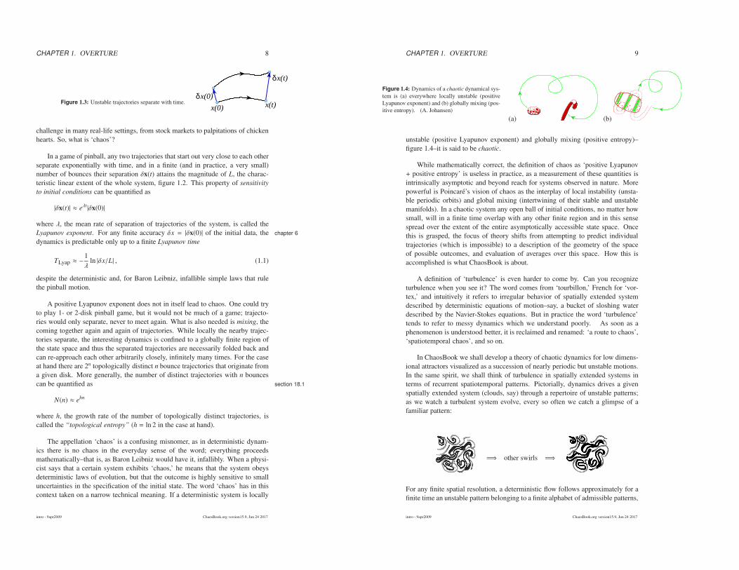
Figure 1.3: Unstable trajectories separate with time. x(0)δ

x(t)δ

x(t)x(0)

challenge in many real-life settings, from stock markets to palpitations of chickenhearts. So, what is ‘chaos’?

In a game of pinball, any two trajectories that start out very close to each otherseparate exponentially with time, and in a finite (and in practice, a very small)number of bounces their separation δx(t) attains the magnitude of L, the charac-teristic linear extent of the whole system, figure 1.2. This property of sensitivity

to initial conditions can be quantified as

|δx(t)| ≈ eλt |δx(0)|

where λ, the mean rate of separation of trajectories of the system, is called theLyapunov exponent. For any finite accuracy δx = |δx(0)| of the initial data, the chapter 6

dynamics is predictable only up to a finite Lyapunov time

TLyap ≈ −1λ

ln |δx/L| , (1.1)

despite the deterministic and, for Baron Leibniz, infallible simple laws that rulethe pinball motion.

A positive Lyapunov exponent does not in itself lead to chaos. One could tryto play 1- or 2-disk pinball game, but it would not be much of a game; trajecto-ries would only separate, never to meet again. What is also needed is mixing, thecoming together again and again of trajectories. While locally the nearby trajec-tories separate, the interesting dynamics is confined to a globally finite region ofthe state space and thus the separated trajectories are necessarily folded back andcan re-approach each other arbitrarily closely, infinitely many times. For the caseat hand there are 2n topologically distinct n bounce trajectories that originate froma given disk. More generally, the number of distinct trajectories with n bouncescan be quantified as section 18.1

N(n) ≈ ehn

where h, the growth rate of the number of topologically distinct trajectories, iscalled the “topological entropy” (h = ln 2 in the case at hand).

The appellation ‘chaos’ is a confusing misnomer, as in deterministic dynam-ics there is no chaos in the everyday sense of the word; everything proceedsmathematically–that is, as Baron Leibniz would have it, infallibly. When a physi-cist says that a certain system exhibits ‘chaos,’ he means that the system obeysdeterministic laws of evolution, but that the outcome is highly sensitive to smalluncertainties in the specification of the initial state. The word ‘chaos’ has in thiscontext taken on a narrow technical meaning. If a deterministic system is locally



Figure 1.4: Dynamics of a chaotic dynamical sys-tem is (a) everywhere locally unstable (positiveLyapunov exponent) and (b) globally mixing (pos-itive entropy). (A. Johansen)

(a) (b)

unstable (positive Lyapunov exponent) and globally mixing (positive entropy)–figure 1.4–it is said to be chaotic.

While mathematically correct, the definition of chaos as ‘positive Lyapunov+ positive entropy’ is useless in practice, as a measurement of these quantities isintrinsically asymptotic and beyond reach for systems observed in nature. Morepowerful is Poincare’s vision of chaos as the interplay of local instability (unsta-ble periodic orbits) and global mixing (intertwining of their stable and unstablemanifolds). In a chaotic system any open ball of initial conditions, no matter howsmall, will in a finite time overlap with any other finite region and in this sensespread over the extent of the entire asymptotically accessible state space. Oncethis is grasped, the focus of theory shifts from attempting to predict individualtrajectories (which is impossible) to a description of the geometry of the spaceof possible outcomes, and evaluation of averages over this space. How this isaccomplished is what ChaosBook is about.

A definition of ‘turbulence’ is even harder to come by. Can you recognizeturbulence when you see it? The word comes from ‘tourbillon,’ French for ‘vor-tex,’ and intuitively it refers to irregular behavior of spatially extended systemdescribed by deterministic equations of motion–say, a bucket of sloshing waterdescribed by the Navier-Stokes equations. But in practice the word ‘turbulence’tends to refer to messy dynamics which we understand poorly. As soon as aphenomenon is understood better, it is reclaimed and renamed: ‘a route to chaos’,‘spatiotemporal chaos’, and so on.

In ChaosBook we shall develop a theory of chaotic dynamics for low dimens-ional attractors visualized as a succession of nearly periodic but unstable motions.In the same spirit, we shall think of turbulence in spatially extended systems interms of recurrent spatiotemporal patterns. Pictorially, dynamics drives a givenspatially extended system (clouds, say) through a repertoire of unstable patterns;as we watch a turbulent system evolve, every so often we catch a glimpse of afamiliar pattern:

=⇒ other swirls =⇒

For any finite spatial resolution, a deterministic flow follows approximately for afinite time an unstable pattern belonging to a finite alphabet of admissible patterns,



and the long term dynamics can be thought of as a walk through the space of suchpatterns. In ChaosBook we recast this image into mathematics.

1.3.2 When does ‘chaos’ matter?

In dismissing Pollock’s fractals because of their limitedmagnification range, Jones-Smith and Mathur would alsodismiss half the published investigations of physical frac-tals.

— Richard P. Taylor [1.4, 1.5]

When should we be mindful of chaos? The solar system is ‘chaotic’, yet wehave no trouble keeping track of the annual motions of planets. The rule of thumbis this; if the Lyapunov time (1.1)–the time by which a state space region initiallycomparable in size to the observational accuracy extends across the entire acces-sible state space–is significantly shorter than the observational time, you need tomaster the theory that will be developed here. That is why the main successes ofthe theory are in statistical mechanics, quantum mechanics, and questions of longterm stability in celestial mechanics.

In science popularizations too much has been made of the impact of ‘chaostheory,’ so a number of caveats are already needed at this point.

At present the theory that will be developed here is in practice applicable onlyto systems of a low intrinsic dimension – the minimum number of coordinates nec-essary to capture its essential dynamics. If the system is very turbulent (a descrip-tion of its long time dynamics requires a space of high intrinsic dimension) we areout of luck. Hence insights that the theory offers in elucidating problems of fullydeveloped turbulence, quantum field theory of strong interactions and early cos-mology have been modest at best. Even that is a caveat with qualifications. Thereare applications–such as spatially extended (non-equilibrium) systems, plumber’sturbulent pipes, etc.,–where the few important degrees of freedom can be isolatedand studied profitably by methods to be described here.

Thus far the theory has had limited practical success when applied to the verynoisy systems so important in the life sciences and in economics. Even thoughwe are often interested in phenomena taking place on time scales much longerthan the intrinsic time scale (neuronal inter-burst intervals, cardiac pulses, etc.),disentangling ‘chaotic’ motions from the environmental noise has been very hard.

In 1980’s something happened that might be without parallel; this is an areaof science where the advent of cheap computation had actually subtracted fromour collective understanding. The computer pictures and numerical plots of frac-tal science of the 1980’s have overshadowed the deep insights of the 1970’s, andthese pictures have since migrated into textbooks. By a regrettable oversight,ChaosBook has none, so ‘Untitled 5’ of figure 1.5 will have to do as the illustra-tion of the power of fractal analysis. Fractal science posits that certain quantities remark 1.7



Figure 1.5: Katherine Jones-Smith, ‘Untitled 5,’ thedrawing used by K. Jones-Smith and R.P. Taylor to testthe fractal analysis of Pollock’s drip paintings [1.6].

(Lyapunov exponents, generalized dimensions, . . . ) can be estimated on a com-puter. While some of the numbers so obtained are indeed mathematically sensiblecharacterizations of fractals, they are in no sense observable and measurable onthe length-scales and time-scales dominated by chaotic dynamics.

Even though the experimental evidence for the fractal geometry of nature iscircumstantial [1.7], in studies of probabilistically assembled fractal aggregateswe know of nothing better than contemplating such quantities. In deterministicsystems we can do much better.

1.4 A game of pinball

Formulas hamper the understanding.

—S. Smale

We are now going to get down to the brass tacks. Time to fasten your seat beltsand turn off all electronic devices. But first, a disclaimer: If you understand therest of this chapter on the first reading, you either do not need this book, or you aredelusional. If you do not understand it, it is not because the people who figuredall this out first are smarter than you: the most you can hope for at this stage is toget a flavor of what lies ahead. If a statement in this chapter mystifies/intrigues,fast forward to a section indicated by [section ...] on the margin, read only theparts that you feel you need. Of course, we think that you need to learn ALL of it,or otherwise we would not have included it in ChaosBook in the first place.

Confronted with a potentially chaotic dynamical system, our analysis pro-ceeds in three stages; I. diagnose, II. count, III. measure. First, we determinethe intrinsic dimension of the system–the minimum number of coordinates nec-essary to capture its essential dynamics. If the system is very turbulent we are,at present, out of luck. We know only how to deal with the transitional regime



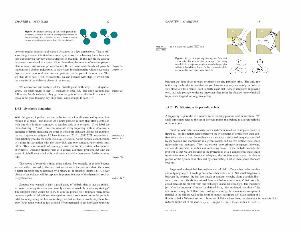
Figure 1.6: Binary labeling of the 3-disk pinball tra-jectories; a bounce in which the trajectory returns tothe preceding disk is labeled 0, and a bounce whichresults in continuation to the third disk is labeled 1.

between regular motions and chaotic dynamics in a few dimensions. That is stillsomething; even an infinite-dimensional system such as a burning flame front canturn out to have a very few chaotic degrees of freedom. In this regime the chaoticdynamics is restricted to a space of low dimension, the number of relevant param-eters is small, and we can proceed to step II; we count and classify all possible chapter 14

chapter 18topologically distinct trajectories of the system into a hierarchy whose successivelayers require increased precision and patience on the part of the observer. Thiswe shall do in sect. 1.4.2. If successful, we can proceed with step III: investigatethe weights of the different pieces of the system.

We commence our analysis of the pinball game with steps I, II: diagnose,count. We shall return to step III–measure–in sect. 1.5. The three sections that chapter 23

follow are highly technical, they go into the guts of what the book is about. Iftoday is not your thinking day, skip them, jump straight to sect. 1.7.

1.4.1 Symbolic dynamics

With the game of pinball we are in luck–it is a low dimensional system, freemotion in a plane. The motion of a point particle is such that after a collisionwith one disk it either continues to another disk or it escapes. If we label thethree disks by 1, 2 and 3, we can associate every trajectory with an itinerary, asequence of labels indicating the order in which the disks are visited; for example,the two trajectories in figure 1.2 have itineraries 2313 , 23132321 respectively. exercise 1.1

section 2.1Such labeling goes by the name symbolic dynamics. As the particle cannot collidetwo times in succession with the same disk, any two consecutive symbols mustdiffer. This is an example of pruning, a rule that forbids certain subsequencesof symbols. Deriving pruning rules is in general a difficult problem, but with thegame of pinball we are lucky–for well-separated disks there are no further pruningrules. chapter 15

The choice of symbols is in no sense unique. For example, as at each bouncewe can either proceed to the next disk or return to the previous disk, the above3-letter alphabet can be replaced by a binary 0, 1 alphabet, figure 1.6. A cleverchoice of an alphabet will incorporate important features of the dynamics, such asits symmetries. section 14.6

Suppose you wanted to play a good game of pinball, that is, get the pinballto bounce as many times as you possibly can–what would be a winning strategy?The simplest thing would be to try to aim the pinball so it bounces many timesbetween a pair of disks–if you managed to shoot it so it starts out in the periodicorbit bouncing along the line connecting two disk centers, it would stay there for-ever. Your game would be just as good if you managed to get it to keep bouncing



Figure 1.7: The 3-disk pinball cycles 12323 and121212313.

Figure 1.8: (a) A trajectory starting out from disk1 can either hit another disk or escape. (b) Hittingtwo disks in a sequence requires a much sharper aim,with initial conditions that hit further consecutive disksnested within each other, as in Fig. 1.9.

between the three disks forever, or place it on any periodic orbit. The only rubis that any such orbit is unstable, so you have to aim very accurately in order tostay close to it for a while. So it is pretty clear that if one is interested in playingwell, unstable periodic orbits are important–they form the skeleton onto which alltrajectories trapped for long times cling.

1.4.2 Partitioning with periodic orbits

A trajectory is periodic if it returns to its starting position and momentum. Weshall sometimes refer to the set of periodic points that belong to a given periodicorbit as a cycle.

Short periodic orbits are easily drawn and enumerated–an example is drawn infigure 1.7–but it is rather hard to perceive the systematics of orbits from their con-figuration space shapes. In mechanics a trajectory is fully and uniquely specifiedby its position and momentum at a given instant, and no two distinct state spacetrajectories can intersect. Their projections onto arbitrary subspaces, however,can and do intersect, in rather unilluminating ways. In the pinball example theproblem is that we are looking at the projections of a 4-dimensional state spacetrajectories onto a 2-dimensional subspace, the configuration space. A clearerpicture of the dynamics is obtained by constructing a set of state space Poincaresections.

Suppose that the pinball has just bounced off disk 1. Depending on its positionand outgoing angle, it could proceed to either disk 2 or 3. Not much happens inbetween the bounces–the ball just travels at constant velocity along a straight line–so we can reduce the 4-dimensional flow to a 2-dimensional map P that takes thecoordinates of the pinball from one disk edge to another disk edge. The trajectoryjust after the moment of impact is defined by sn, the arc-length position of thenth bounce along the billiard wall, and pn = p sin φn the momentum componentparallel to the billiard wall at the point of impact, see figure 1.9. Such section of aflow is called a Poincare section. In terms of Poincare sections, the dynamics is example 15.9

reduced to the set of six maps Psk←s j: (sn, pn) 7→ (sn+1, pn+1), with s ∈ 1, 2, 3,



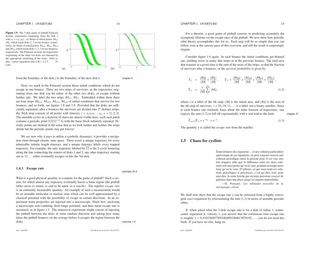
Figure 1.9: The 3-disk game of pinball Poincaresection, trajectories emanating from the disk 1with x0 = (s0, p0) . (a) Strips of initial pointsM12,M13 which reach disks 2, 3 in one bounce, respec-tively. (b) Strips of initial pointsM121,M131M132

andM123 which reach disks 1, 2, 3 in two bounces,respectively. The Poincare sections for trajectoriesoriginating on the other two disks are obtained bythe appropriate relabeling of the strips. Disk ra-dius : center separation ratio a:R = 1:2.5. (Y.Lan)

(a)

sin

Ø

1

0

−1

−2.5

S

0 2.5

1312

(b)

−1

0

sinØ

1

2.50s

−2.5

132

131123

121

from the boundary of the disk j to the boundary of the next disk k. chapter 9

Next, we mark in the Poincare section those initial conditions which do notescape in one bounce. There are two strips of survivors, as the trajectories orig-inating from one disk can hit either of the other two disks, or escape withoutfurther ado. We label the two strips M12, M13. Embedded within them thereare four stripsM121,M123,M131,M132 of initial conditions that survive for twobounces, and so forth, see figures 1.8 and 1.9. Provided that the disks are suffi-ciently separated, after n bounces the survivors are divided into 2n distinct strips:the Mith strip consists of all points with itinerary i = s1s2s3 . . . sn, s = 1, 2, 3.The unstable cycles as a skeleton of chaos are almost visible here: each such patchcontains a periodic point s1s2s3 . . . sn with the basic block infinitely repeated. Pe-riodic points are skeletal in the sense that as we look further and further, the stripsshrink but the periodic points stay put forever.

We see now why it pays to utilize a symbolic dynamics; it provides a naviga-tion chart through chaotic state space. There exists a unique trajectory for everyadmissible infinite length itinerary, and a unique itinerary labels every trappedtrajectory. For example, the only trajectory labeled by 12 is the 2-cycle bouncingalong the line connecting the centers of disks 1 and 2; any other trajectory startingout as 12 . . . either eventually escapes or hits the 3rd disk.

1.4.3 Escape rateexample 20.4

What is a good physical quantity to compute for the game of pinball? Such a sys-tem, for which almost any trajectory eventually leaves a finite region (the pinballtable) never to return, is said to be open, or a repeller. The repeller escape rate

is an eminently measurable quantity. An example of such a measurement wouldbe an unstable molecular or nuclear state which can be well approximated by aclassical potential with the possibility of escape in certain directions. In an ex-periment many projectiles are injected into a macroscopic ‘black box’ enclosinga microscopic non-confining short-range potential, and their mean escape rate ismeasured, as in figure 1.1. The numerical experiment might consist of injectingthe pinball between the disks in some random direction and asking how manytimes the pinball bounces on the average before it escapes the region between thedisks. exercise 1.2



For a theorist, a good game of pinball consists in predicting accurately theasymptotic lifetime (or the escape rate) of the pinball. We now show how periodicorbit theory accomplishes this for us. Each step will be so simple that you canfollow even at the cursory pace of this overview, and still the result is surprisinglyelegant.

Consider figure 1.9 again. In each bounce the initial conditions get thinnedout, yielding twice as many thin strips as at the previous bounce. The total areathat remains at a given time is the sum of the areas of the strips, so that the fractionof survivors after n bounces, or the survival probability is given by

Γ1 =|M0|

|M|+|M1|

|M|, Γ2 =

|M00|

|M|+|M10|

|M|+|M01|

|M|+|M11|

|M|,

Γn =1|M|

(n)∑

i

|Mi| , (1.2)

where i is a label of the ith strip, |M| is the initial area, and |Mi| is the area ofthe ith strip of survivors. i = 01, 10, 11, . . . is a label, not a binary number. Sinceat each bounce one routinely loses about the same fraction of trajectories, oneexpects the sum (1.2) to fall off exponentially with n and tend to the limit chapter 27

Γn+1/Γn = e−γn → e−γ. (1.3)

The quantity γ is called the escape rate from the repeller.

1.5 Chaos for cyclists

Etant donnees des equations ... et une solution particulierequelconque de ces equations, on peut toujours trouver unesolution periodique (dont la periode peut, il est vrai, etretres longue), telle que la difference entre les deux solu-tions soit aussi petite qu’on le veut, pendant un temps aussilong qu’on le veut. D’ailleurs, ce qui nous rend ces solu-tions periodiques si precieuses, c’est qu’elles sont, pouransi dire, la seule breche par ou nous puissions esseyer depenetrer dans une place jusqu’ici reputee inabordable.

—H. Poincare, Les methodes nouvelles de la

mechanique celeste

We shall now show that the escape rate γ can be extracted from a highly conver-gent exact expansion by reformulating the sum (1.2) in terms of unstable periodicorbits.

If, when asked what the 3-disk escape rate is for a disk of radius 1, center-center separation 6, velocity 1, you answer that the continuous time escape rateis roughly γ = 0.4103384077693464893384613078192 . . . , you do not need thisbook. If you have no clue, hang on.



Figure 1.10: The Jacobian matrix Jt maps an infinites-imal displacement δx at x0 into a displacement Jt(x0)δxa finite time t later.

δ x(t) = J tδ x(0)

x(0)δ

x(0)

x(t)

1.5.1 How big is my neighborhood?

Of course, we can prove all these results directly fromEq. (20.25) by pedestrian mathematical manipulations,but that only makes it harder to appreciate their physicalsignificance.

— Rick Salmon, “Lectures on Geophysical Fluid Dy-namics”, Oxford Univ. Press (1998)

Not only do the periodic points keep track of topological ordering of the strips,but, as we shall now show, they also determine their size. As a trajectory evolves,it carries along and distorts its infinitesimal neighborhood. Let

x(t) = f t(x0)

denote the trajectory of an initial point x0 = x(0). Expanding f t(x0 + δx0) tolinear order, the evolution of the distance to a neighboring trajectory x(t) + δx(t)is given by the Jacobian matrix J:

δxi(t) =d

∑

j=1

Jt(x0)i jδx0 j , Jt(x0)i j =∂xi(t)∂x0 j

. (1.4)

A trajectory of a pinball moving on a flat surface is specified by two positioncoordinates and the direction of motion, so in this case d = 3. Evaluation ofa cycle Jacobian matrix is a long exercise - here we just state the result. The section 9.2

Jacobian matrix describes the deformation of an infinitesimal neighborhood ofx(t) along the flow; its eigenvectors and eigenvalues give the directions and thecorresponding rates of expansion or contraction, figure 1.10. The trajectories thatstart out in an infinitesimal neighborhood separate along the unstable directions(those whose eigenvalues are greater than unity in magnitude), approach eachother along the stable directions (those whose eigenvalues are less than unity inmagnitude), and change their distance only sub-exponentially (or not at all) alongthe marginal directions (those whose eigenvalues equal unity in magnitude).

In our game of pinball the beam of neighboring trajectories is defocused alongthe unstable eigen-direction of the Jacobian matrix J.

As the heights of the strips in figure 1.9 are effectively constant, we can con-centrate on their thickness. If the height is ≈ L, then the area of the ith strip isMi ≈ Lli for a strip of width li.



Each strip i in figure 1.9 contains a periodic point xi. The finer the intervals,the smaller the variation in flow across them, so the contribution from the stripof width li is well-approximated by the contraction around the periodic point xi

within the interval,

li = ai/|Λi| , (1.5)

where Λi is the unstable eigenvalue of the Jacobian matrix Jt(xi) evaluated atthe ith periodic point for t = Tp, the full period (due to the low dimensionality,the Jacobian can have at most one unstable eigenvalue). Only the magnitude ofthis eigenvalue matters, we can disregard its sign. The prefactors ai reflect theoverall size of the system and the particular distribution of starting values of x. Asthe asymptotic trajectories are strongly mixed by bouncing chaotically around therepeller, we expect their distribution to be insensitive to smooth variations in thedistribution of initial points. section 19.4

To proceed with the derivation we need the hyperbolicity assumption: forlarge n the prefactors ai ≈ O(1) are overwhelmed by the exponential growth ofΛi, so we neglect them. If the hyperbolicity assumption is justified, we can replace section 21.1.1

|Mi| ≈ Lli in (1.2) by 1/|Λi| and consider the sum

Γn =

(n)∑

i

1/|Λi| ,

where the sum goes over all periodic points of period n. We now define a gener-ating function for sums over all periodic orbits of all lengths:

Γ(z) =∞∑

n=1

Γnzn . (1.6)

Recall that for large n the nth level sum (1.2) tends to the limit Γn → e−nγ, so theescape rate γ is determined by the smallest z = eγ for which (1.6) diverges:

Γ(z) ≈∞∑

n=1

(ze−γ)n=

ze−γ

1 − ze−γ. (1.7)

This is the property of Γ(z) that motivated its definition. Next, we devise a formulafor (1.6) expressing the escape rate in terms of periodic orbits:

Γ(z) =∞∑

n=1

zn

(n)∑

i

|Λi|−1

=z

|Λ0|+

z

|Λ1|+

z2

|Λ00|+

z2

|Λ01|+

z2

|Λ10|+

z2

|Λ11|

+z3

|Λ000|+

z3

|Λ001|+

z3

|Λ010|+

z3

|Λ100|+ . . . (1.8)

For sufficiently small z this sum is convergent. The escape rate γ is now given by section 21.3

the leading pole of (1.7), rather than by a numerical extrapolation of a sequence of



γn extracted from (1.3). As any finite truncation n < ntrunc of (1.8) is a polyno-mial in z, convergent for any z, finding this pole requires that we know somethingabout Γn for any n, and that might be a tall order.

We could now proceed to estimate the location of the leading singularity ofΓ(z) from finite truncations of (1.8) by methods such as Pade approximants. How-ever, as we shall now show, it pays to first perform a simple resummation thatconverts this divergence into a zero of a related function.

1.5.2 Dynamical zeta function

If a trajectory retraces a prime cycle r times, its expanding eigenvalue is Λrp. A

prime cycle p is a single traversal of the orbit; its label is a non-repeating symbolstring of np symbols. There is only one prime cycle for each cyclic permutationclass. For example, p = 0011 = 1001 = 1100 = 0110 is prime, but 0101 = 01 is not.By the chain rule for derivatives the stability of a cycle is the same everywhere exercise 18.2

section 4.5along the orbit, so each prime cycle of length np contributes np terms to the sum(1.8). Hence (1.8) can be rewritten as

Γ(z) =∑

p

np

∞∑

r=1

(

znp

|Λp|

)r

=∑

p

nptp

1 − tp

, tp =znp

|Λp|(1.9)

where the index p runs through all distinct prime cycles. Note that we have re-summed the contribution of the cycle p to all times, so truncating the summationup to given p is not a finite time n ≤ np approximation, but an asymptotic, infinite

time estimate based by approximating stabilities of all cycles by a finite number ofthe shortest cycles and their repeats. The npznp factors in (1.9) suggest rewritingthe sum as a derivative

Γ(z) = −zd

dz

∑

p

ln(1 − tp) .

Hence Γ(z) is z× derivative derivative of the logarithm of the infinite product

1/ζ(z) =∏

p

(1 − tp) , tp =znp

|Λp|. (1.10)

This function is called the dynamical zeta function, in analogy to the Riemannzeta function, which motivates the ‘zeta’ in its definition as 1/ζ(z). This is theprototype formula of periodic orbit theory. The zero of 1/ζ(z) is a pole of Γ(z),and the problem of estimating the asymptotic escape rates from finite n sumssuch as (1.2) is now reduced to a study of the zeros of the dynamical zeta function(1.10). The escape rate is related by (1.7) to a divergence of Γ(z), and Γ(z) diverges section 27.1

whenever 1/ζ(z) has a zero. section 22.4

Easy, you say: “Zeros of (1.10) can be read off the formula, a zero

zp = |Λp|1/np

for each term in the product. What’s the problem?” Dead wrong!



1.5.3 Cycle expansions

How are formulas such as (1.10) used? We start by computing the lengths andeigenvalues of the shortest cycles. This usually requires some numerical work,such as the Newton method searches for periodic solutions; we shall assume thatthe numerics are under control, and that all short cycles up to given length havebeen found. In our pinball example this can be done by elementary geometrical chapter 16

optics. It is very important not to miss any short cycles, as the calculation is asaccurate as the shortest cycle dropped–including cycles longer than the shortestomitted does not improve the accuracy. The result of such numerics is a table ofthe shortest cycles, their periods and their stabilities. section 33.3

Now expand the infinite product (1.10), grouping together the terms of thesame total symbol string length

1/ζ = (1 − t0)(1 − t1)(1 − t10)(1 − t100) · · ·

= 1 − t0 − t1 − [t10 − t1t0] − [(t100 − t10t0) + (t101 − t10t1)]

−[(t1000 − t0t100) + (t1110 − t1t110)

+(t1001 − t1t001 − t101t0 + t10t0t1)] − . . . (1.11)

The virtue of the expansion is that the sum of all terms of the same total length chapter 23

n (grouped in brackets above) is a number that is exponentially smaller than atypical term in the sum, for geometrical reasons we explain in the next section. section 23.1

The calculation is now straightforward. We substitute a finite set of the eigen-values and lengths of the shortest prime cycles into the cycle expansion (1.11), andobtain a polynomial approximation to 1/ζ. We then vary z in (1.10) and determinethe escape rate γ by finding the smallest z = eγ for which (1.11) vanishes.

1.5.4 Shadowing

When you actually start computing this escape rate, you will find out that theconvergence is very impressive: only three input numbers (the two fixed points 0,1 and the 2-cycle 10) already yield the pinball escape rate to 3-4 significant digits!We have omitted an infinity of unstable cycles; so why does approximating the section 23.2.2

dynamics by a finite number of the shortest cycle eigenvalues work so well?

The convergence of cycle expansions of dynamical zeta functions is a conse-quence of the smoothness and analyticity of the underlying flow. Intuitively, onecan understand the convergence in terms of the geometrical picture sketched infigure 1.11; the key observation is that the long orbits are shadowed by sequencesof shorter orbits.

A typical term in (1.11) is a difference of a long cycle abminus its shadowingapproximation by shorter cycles a and b (see figure 1.12),

tab − tatb = tab(1 − tatb/tab) = tab

(

1 −∣

∣

∣

∣

∣

Λab

ΛaΛb

∣

∣

∣

∣

∣

)

, (1.12)



Figure 1.11: Approximation to a smooth dynamics(left frame) by the skeleton of periodic points, togetherwith their linearized neighborhoods, (right frame). In-dicated are segments of two 1-cycles and a 2-cyclethat alternates between the neighborhoods of the two1-cycles, shadowing first one of the two 1-cycles, andthen the other.

Figure 1.12: A longer cycle p′′ shadowed by a pair (a‘pseudo orbit’) of shorter cycles p and p′.

p

p"p’

where a and b are symbol sequences of the two shorter cycles. If all orbits areweighted equally (tp = znp ), such combinations cancel exactly; if orbits of similarsymbolic dynamics have similar weights, the weights in such combinations almostcancel.

This can be understood in the context of the pinball game as follows. Considerorbits 0, 1 and 01. The first corresponds to bouncing between any two disks whilethe second corresponds to bouncing successively around all three, tracing out anequilateral triangle. The cycle 01 starts at one disk, say disk 2. It then bouncesfrom disk 3 back to disk 2 then bounces from disk 1 back to disk 2 and so on, so itsitinerary is 2321. In terms of the bounce types shown in figure 1.6, the trajectory isalternating between 0 and 1. The incoming and outgoing angles when it executesthese bounces are very close to the corresponding angles for 0 and 1 cycles. Alsothe distances traversed between bounces are similar so that the 2-cycle expandingeigenvalue Λ01 is close in magnitude to the product of the 1-cycle eigenvaluesΛ0Λ1.

To understand this on a more general level, try to visualize the partition ofa chaotic dynamical system’s state space in terms of cycle neighborhoods as atessellation (a tiling) of the dynamical system, with smooth flow approximated byits periodic orbit skeleton, each ‘tile’ centered on a periodic point, and the scaleof the ‘tile’ determined by the linearization of the flow around the periodic point,as illustrated by figure 1.11.

The orbits that follow the same symbolic dynamics, such as ab and a ‘pseudoorbit’ ab (see figure 1.12), lie close to each other in state space; long shadow-ing pairs have to start out exponentially close to beat the exponential growth inseparation with time. If the weights associated with the orbits are multiplicativealong the flow (for example, by the chain rule for products of derivatives) andthe flow is smooth, the term in parenthesis in (1.12) falls off exponentially with



the cycle length, and therefore the curvature expansions are expected to be highlyconvergent. chapter 28

1.6 Change in time

MEN are deplorably ignorant with respect to naturalthings and modern philosophers as though dreaming in thedarkness must be aroused and taught the uses of things thedealing with things they must be made to quit the sort oflearning that comes only from books and that rests onlyon vain arguments from probability and upon conjectures.

— William Gilbert, De Magnete, 1600

The above derivation of the dynamical zeta function formula for the escape ratehas one shortcoming; it estimates the fraction of survivors as a function of thenumber of pinball bounces, but the physically interesting quantity is the escaperate measured in units of continuous time. For continuous time flows, the escaperate (1.2) is generalized as follows. Define a finite state space region M suchthat a trajectory that exits M never reenters. For example, any pinball that fallsof the edge of a pinball table in figure 1.1 is gone forever. Start with a uniformdistribution of initial points. The fraction of initial x whose trajectories remainwithinM at time t is expected to decay exponentially

Γ(t) =

∫

Mdxdy δ(y − f t(x))

∫

Mdx

→ e−γt .

The integral over x starts a trajectory at every x ∈ M. The integral over y testswhether this trajectory is still inM at time t. The kernel of this integral

Lt(y, x) = δ(

y − f t(x))

(1.13)

is the Dirac delta function, as for a deterministic flow the initial point x mapsinto a unique point y at time t. For discrete time, f n(x) is the nth iterate of themap f . For continuous flows, f t(x) is the trajectory of the initial point x, and itis appropriate to express the finite time kernel Lt in terms of A, the generator ofinfinitesimal time translations

Lt = etA ,

very much in the way the quantum evolution is generated by the Hamiltonian H, section 19.6

the generator of infinitesimal time quantum transformations.

As the kernel L is the key to everything that follows, we shall give it a name,and refer to it and its generalizations as the evolution operator for a d-dimensionalmap or a d-dimensional flow.

The number of periodic points increases exponentially with the cycle length(in the case at hand, as 2n). As we have already seen, this exponential proliferation



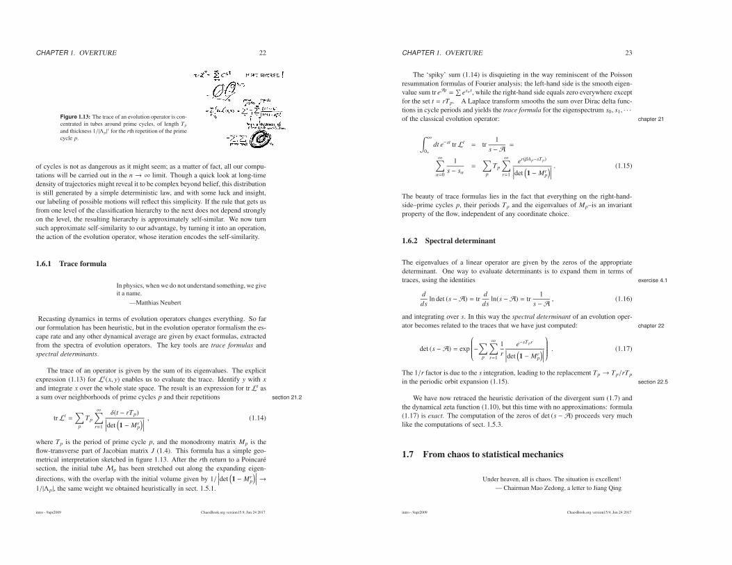
Figure 1.13: The trace of an evolution operator is con-centrated in tubes around prime cycles, of length Tp

and thickness 1/|Λp|r for the rth repetition of the prime

cycle p.

of cycles is not as dangerous as it might seem; as a matter of fact, all our compu-tations will be carried out in the n → ∞ limit. Though a quick look at long-timedensity of trajectories might reveal it to be complex beyond belief, this distributionis still generated by a simple deterministic law, and with some luck and insight,our labeling of possible motions will reflect this simplicity. If the rule that gets usfrom one level of the classification hierarchy to the next does not depend stronglyon the level, the resulting hierarchy is approximately self-similar. We now turnsuch approximate self-similarity to our advantage, by turning it into an operation,the action of the evolution operator, whose iteration encodes the self-similarity.

1.6.1 Trace formula

In physics, when we do not understand something, we giveit a name.

—Matthias Neubert

Recasting dynamics in terms of evolution operators changes everything. So farour formulation has been heuristic, but in the evolution operator formalism the es-cape rate and any other dynamical average are given by exact formulas, extractedfrom the spectra of evolution operators. The key tools are trace formulas andspectral determinants.

The trace of an operator is given by the sum of its eigenvalues. The explicitexpression (1.13) for Lt(x, y) enables us to evaluate the trace. Identify y with x

and integrate x over the whole state space. The result is an expression for trLt asa sum over neighborhoods of prime cycles p and their repetitions section 21.2

trLt =∑

p

Tp

∞∑

r=1

δ(t − rTp)∣

∣

∣

∣

det(

1 − Mrp

)

∣

∣

∣

∣

, (1.14)

where Tp is the period of prime cycle p, and the monodromy matrix Mp is theflow-transverse part of Jacobian matrix J (1.4). This formula has a simple geo-metrical interpretation sketched in figure 1.13. After the rth return to a Poincaresection, the initial tube Mp has been stretched out along the expanding eigen-

directions, with the overlap with the initial volume given by 1/∣

∣

∣

∣

det(

1 − Mrp

)

∣

∣

∣

∣

→

1/|Λp|, the same weight we obtained heuristically in sect. 1.5.1.



The ‘spiky’ sum (1.14) is disquieting in the way reminiscent of the Poissonresummation formulas of Fourier analysis; the left-hand side is the smooth eigen-value sum tr eAt =

∑

esαt, while the right-hand side equals zero everywhere exceptfor the set t = rTp. A Laplace transform smooths the sum over Dirac delta func-tions in cycle periods and yields the trace formula for the eigenspectrum s0, s1, · · ·

of the classical evolution operator: chapter 21

∫ ∞

0+dt e−st trLt = tr

1s −A

=

∞∑

α=0

1s − sα

=∑

p

Tp

∞∑

r=1

er(βAp−sTp)∣

∣

∣

∣

det(

1 − Mrp

)

∣

∣

∣

∣

. (1.15)

The beauty of trace formulas lies in the fact that everything on the right-hand-side–prime cycles p, their periods Tp and the eigenvalues of Mp–is an invariantproperty of the flow, independent of any coordinate choice.

1.6.2 Spectral determinant

The eigenvalues of a linear operator are given by the zeros of the appropriatedeterminant. One way to evaluate determinants is to expand them in terms oftraces, using the identities exercise 4.1

d

dsln det (s −A) = tr

d

dsln(s − A) = tr

1s −A

, (1.16)

and integrating over s. In this way the spectral determinant of an evolution oper-ator becomes related to the traces that we have just computed: chapter 22

det (s −A) = exp

−∑

p

∞∑

r=1

1r

e−sTpr

∣

∣

∣

∣

det(

1 − Mrp

)

∣

∣

∣

∣

. (1.17)

The 1/r factor is due to the s integration, leading to the replacement Tp → Tp/rTp

in the periodic orbit expansion (1.15). section 22.5

We have now retraced the heuristic derivation of the divergent sum (1.7) andthe dynamical zeta function (1.10), but this time with no approximations: formula(1.17) is exact. The computation of the zeros of det (s − A) proceeds very muchlike the computations of sect. 1.5.3.

1.7 From chaos to statistical mechanics

Under heaven, all is chaos. The situation is excellent!— Chairman Mao Zedong, a letter to Jiang Qing



The replacement of individual trajectories by evolution operators which propa-gate densities feels like a bit of voodoo. Nevertheless, something very radical anddeeply foundational has taken place. Understanding the distinction between evo-lution of individual trajectories and the evolution of the densities of trajectories iskey to understanding statistical mechanics–this is the conceptual basis of the sec-ond law of thermodynamics, and the origin of irreversibility of the arrow of timefor deterministic systems with time-reversible equations of motion: reversibility isattainable for distributions whose measure in the space of density functions goesexponentially to zero with time.

Consider a chaotic flow, such as the stirring of red and white paint by somedeterministic machine. If we were able to track individual trajectories, the fluidwould forever remain a striated combination of pure white and pure red; therewould be no pink. What is more, if we reversed the stirring, we would return tothe perfect white/red separation. However, that cannot be–in a very few turns ofthe stirring stick the thickness of the layers goes from centimeters to Ångstroms,and the result is irreversibly pink.

A century ago it seemed reasonable to assume that statistical mechanics ap-plies only to systems with very many degrees of freedom. More recent is therealization that much of statistical mechanics follows from chaotic dynamics, andalready at the level of a few degrees of freedom the evolution of densities is irre-versible. Furthermore, the theory that we shall develop here generalizes notions of‘measure’ and ‘averaging’ to systems far from equilibrium, and transports us intoregions hitherto inaccessible with the tools of equilibrium statistical mechanics.

By going to a description in terms of the asymptotic time evolution operatorswe give up tracking individual trajectories for long times, but trade in the un-controllable trajectories for a powerful description of the asymptotic trajectorydensities. This will enable us, for example, to give exact formulas for transportcoefficients such as the diffusion constants without any probabilistic assumptions. chapter 24

The classical Boltzmann equation for evolution of 1-particle density is based onstosszahlansatz, neglect of particle correlations prior to, or after a 2-particle col-lision. It is a very good approximate description of dilute gas dynamics, buta difficult starting point for inclusion of systematic corrections. In the theorydeveloped here, no correlations are neglected - they are all included in the cy-cle averaging formulas such as the cycle expansion for the diffusion constant2dD = limT→∞〈x(T )2〉/T of a particle diffusing chaotically across a spatially-periodic array, section 24.1

D =1

2d

1〈T〉ζ

∑′(−1)k+1 (np1 + · · · + npk

)2

|Λp1 · · ·Λpk|, (1.18)

where np is a translation along one period of a spatially periodic ‘runaway’ tra-jectory p. Such formulas are exact; the issue in their applications is what arethe most effective schemes of estimating the infinite cycle sums required for theirevaluation. Unlike most statistical mechanics, here there are no phenomenologicalmacroscopic parameters; quantities such as transport coefficients are calculable toany desired accuracy from the microscopic dynamics.



Figure 1.14: (a) Washboard mean velocity, (b)cold atom lattice diffusion, and (c) AFM tip dragforce. (Y. Lan)

(a)Θ

(b) ωsin( t)

(c) velocity

frequency Ω

The concepts of equilibrium statistical mechanics do help us, however, to un-derstand the ways in which the simple-minded periodic orbit theory falters. Anon-hyperbolicity of the dynamics manifests itself in power-law correlations and chapter 29

even ‘phase transitions.’

1.8 Chaos: what is it good for?

Happy families are all alike; every unhappy family is un-happy in its own way.

— Anna Karenina, by Leo Tolstoy

With initial data accuracy δx = |δx(0)| and system size L, a trajectory is predictableonly up to the finite Lyapunov time (1.1), TLyap ≈ λ

−1 ln |L/δx| . Beyond that,chaos rules. And so the most successful applications of ‘chaos theory’ have so farbeen to problems where observation time is much longer than a typical ‘turnover’time, such as statistical mechanics, quantum mechanics, and questions of longterm stability in celestial mechanics, where the notion of tracking accurately agiven state of the system is nonsensical.

So what is chaos good for? Transport! Though superficially indistinguishablefrom the probabilistic random walk diffusion, in low dimensional settings the de-terministic diffusion is quite recognizable, through the fractal dependence of thediffusion constant on the system parameters, and perhaps through non-Gaussionrelaxation to equilibrium (non-vanishing Burnett coefficients). section 24.2.1



Several tabletop experiments that could measure transport on macroscopicscales are sketched in figure 1.14 (each a tabletop, but an expensive tabletop). Fig-ure 1.14 (a) depicts a ‘slanted washboard;’ a particle in a gravity field bouncingdown the washboard, losing some energy at each bounce, or a charged particle ina constant electric field trickling across a periodic condensed-matter device. Theinterplay between chaotic dynamics and energy loss results in a terminal mean ve-locity/conductance, a function of the washboard slant or external electric field thatthe periodic theory can predict accurately. Figure 1.14 (b) depicts a ‘cold atom lat-tice’ of very accurate spatial periodicity, with a dilute cloud of atoms placed ontoa standing wave established by strong laser fields. Interaction of gravity with gen-tle time-periodic jiggling of the EM fields induces a diffusion of the atomic cloud,with a diffusion constant predicted by the periodic orbit theory. Figure 1.14 (c)depicts a tip of an atomic force microscope (AFM) bouncing against a periodicatomic surface moving at a constant velocity. The frictional drag experiencedis the interplay of the chaotic bouncing of the tip and the energy loss at eachtip/surface collision, accurately predicted by the periodic orbit theory. None of ChaosBook.org/projects

these experiments have actually been carried out, (save for some numerical exper-imentation), but are within reach of what can be measured today.

Given microscopic dynamics, periodic orbit theory predicts observable macro-scopic transport quantities such as the washboard mean velocity, cold atom latticediffusion constant, and AFM tip drag force. But the experimental proposal is sex-ier than that, and goes into the heart of dynamical systems theory. remark A1.1

Smale 1960s theory of the hyperbolic structure of the non–wandering set(AKA ‘horseshoe’) was motivated by his ‘structural stability’ conjecture, which -in non-technical terms - asserts that all trajectories of a chaotic dynamical systemdeform smoothly under small variations of system parameters.

Why this cannot be true for a system like the washboard in figure 1.14 (a) iseasy to see for a cyclist. Take a trajectory which barely grazes the tip of one of thegroves. An arbitrarily small change in the washboard slope can result in loss ofthis collision, change a forward scattering into a backward scattering, and lead toa discontinuous contribution to the mean velocity. You might hold out hope thatsuch events are rare and average out, but not so - a loss of a short cycle leads to asignificant change in the cycle-expansion formula for a transport coefficient, suchas (1.18).

When we write an equation, it is typically parameterized by a set of parametersby as coupling strengths, and we think of dynamical systems obtained by a smoothvariation of a parameter as a ‘family.’ We would expect measurable predictions toalso vary smoothly, i.e., be ‘structurally stable.’

But dynamical systems families are ‘families’ only in a name. That the struc-tural stability conjecture turned out to be badly wrong is, however, not a blow forchaotic dynamics. Quite to the contrary, it is actually a virtue, perhaps the most section 15.2

dramatic experimentally measurable prediction of chaotic dynamics.

As long as microscopic periodicity is exact, the prediction is counterintuitivefor a physicist - transport coefficients are not smooth functions of system parame- section 24.2



ters, rather they are non-monotonic, nowhere differentiable functions. Conversely,if the macroscopic measurement yields a smooth dependence of the transport onsystem parameters, the periodicity of the microscopic lattice is degraded by impu-rities, and probabilistic assumptions of traditional statistical mechanics apply. Sothe proposal is to –by measuring macroscopic transport– conductance, diffusion,drag –observe determinism on nanoscales, and –for example– determine whetheran atomic surface is clean.

The signatures of deterministic chaos are even more baffling to an engineer:a small increase of pressure across a pipe exhibiting turbulent flow does not nec-essarily lead to an increase in the mean flow; mean flow dependence on pressuredrop across the pipe is also a fractal function.

Is this in contradiction with the traditional statistical mechanics? No - deter-ministic chaos predictions are valid in settings where a few degrees of freedom areimportant, and chaotic motion time and space scales are commensurate with theexternal driving and spatial scales. Further degrees of freedom act as noise thatsmooths out the above fractal effects and restores a smooth functional dependenceof transport coefficients on external parameters.

1.9 What is not in ChaosBook

There is only one thing which interests me vitally now,and that is the recording of all that which is omitted inbooks. Nobody, as far as I can see, is making use of thoseelements in the air which give direction and motivation toour lives.

— Henry Miller, Tropic of Cancer

This book offers everyman a breach into a domain hitherto reputed unreachable,a domain traditionally traversed only by mathematical physicists and mathemati-cians. What distinguishes it from mathematics is the insistence on computabilityand numerical convergence of methods offered. A rigorous proof, the end of thestory as far as a mathematician is concerned, might state that in a given setting,for times in excess of 1032 years, turbulent dynamics settles onto an attractor ofdimension less than 600. Such a theorem is of a little use to a hard-workingplumber, especially if her hands-on experience is that within the span of a fewtypical ‘turnaround’ times the dynamics seems to settle on a (transient?) attractorof dimension less than 3. If rigor, magic, fractals or brains is your thing, readremark 1.4 and beyond.

So, no proofs! but lot of hands-on plumbing ahead.

Many a chapter alone could easily grow to a book size if unchecked: thenuts and bolt of the theory include ODEs, PDEs, stochastic ODEs, path integrals,group theory, coding theory, graph theory, ergodic theory, linear operator theory,quantum mechanics, etc.. We include material into the text proper on ‘need-to-



know’ basis, relegate technical details to appendices, and give pointers to furtherreading in the remarks at the end of each chapter.

Resume

This text is an exposition of the best of all possible theories of deterministic chaos,and the strategy is: 1) count, 2) weigh, 3) add up.

In a chaotic system any open ball of initial conditions, no matter how small,will spread over the entire accessible state space. Hence the theory focuses ondescribing the geometry of the space of possible outcomes, and evaluating av-erages over this space, rather than attempting the impossible: precise predictionof individual trajectories. The dynamics of densities of trajectories is describedin terms of evolution operators. In the evolution operator formalism the dynami-cal averages are given by exact formulas, extracted from the spectra of evolutionoperators. The key tools are trace formulas and spectral determinants.

The theory of evaluation of the spectra of evolution operators presented here isbased on the observation that the motion in dynamical systems of few degrees offreedom is often organized around a few fundamental cycles. These short cyclescapture the skeletal topology of the motion on a strange attractor/repeller in thesense that any long orbit can approximately be pieced together from the nearby pe-riodic orbits of finite length. This notion is made precise by approximating orbitsby prime cycles, and evaluating the associated curvatures. A curvature measuresthe deviation of a longer cycle from its approximation by shorter cycles; smooth-ness and the local instability of the flow implies exponential (or faster) fall-off for(almost) all curvatures. Cycle expansions offer an efficient method for evaluatingclassical and quantum observables.

The critical step in the derivation of the dynamical zeta function was the hy-perbolicity assumption, i.e., the assumption of exponential shrinkage of all stripsof the pinball repeller. By dropping the ai prefactors in (1.5), we have given up onany possibility of recovering the precise distribution of starting x (which shouldanyhow be impossible due to the exponential growth of errors), but in exchangewe gain an effective description of the asymptotic behavior of the system. Thepleasant surprise of cycle expansions (1.10) is that the infinite time behavior of anunstable system is as easy to determine as the short time behavior.

To keep the exposition simple we have here illustrated the utility of cyclesand their curvatures by a pinball game, but topics covered in ChaosBook – un-stable flows, Poincare sections, Smale horseshoes, symbolic dynamics, pruning,discrete symmetries, periodic orbits, averaging over chaotic sets, evolution oper-ators, dynamical zeta functions, spectral determinants, cycle expansions, quantumtrace formulas, zeta functions, and so on to the semiclassical quantization of he-lium – should give the reader some confidence in the broad sway of the theory.The formalism should work for any average over any chaotic set which satisfiestwo conditions:



1. the weight associated with the observable under consideration is multiplica-tive along the trajectory,

2. the set is organized in such a way that the nearby points in the symbolicdynamics have nearby weights.

The theory is applicable to evaluation of a broad class of quantities characterizingchaotic systems, such as the escape rates, Lyapunov exponents, transport coeffi-cients and quantum eigenvalues. A big surprise is that the semi-classical quantummechanics of systems classically chaotic is very much like the classical mechanicsof chaotic systems; both are described by zeta functions and cycle expansions ofthe same form, with the same dependence on the topology of the classical flow.



But the power of instruction is seldom of much efficacy,except in those happy dispositions where it is almost su-perfluous.

—Gibbon

Commentary

Remark 1.1 Nonlinear dynamics texts. This text aims to bridge the gap between thephysics and mathematics dynamical systems literature. The intended audience is Hen-riette Roux, the perfect physics graduate student with a theoretical bent who does notbelieve anything she is told. As a complementary presentation we recommend Gaspard’smonograph [A1.65] which covers much of the same ground in a highly readable andscholarly manner.

As far as the prerequisites are concerned–ChaosBook is not an introduction to non-linear dynamics. Nonlinear science requires a one semester basic course (advanced un-dergraduate or first year graduate). A good start is the textbook by Strogatz [1.9], anintroduction to the applied mathematician’s visualization of flows, fixed points, mani-folds, bifurcations. It is the most accessible introduction to nonlinear dynamics–a bookon differential equations in nonlinear disguise, and its broadly chosen examples and manyexercises make it a favorite with students. It is not strong on chaos. There the textbookof Alligood, Sauer and Yorke [1.10] is preferable: an elegant introduction to maps, chaos,period doubling, symbolic dynamics, fractals, dimensions–a good companion to Chaos-Book. Introduction more comfortable to physicists is the textbook by Ott [A1.66], withthe baker’s map used to illustrate many key techniques in analysis of chaotic systems. Ottis perhaps harder than the above two as first books on nonlinear dynamics. Sprott [1.12]and Jackson [2.27] textbooks are very useful compendia of the ’70s and onward ‘chaos’literature which we, in the spirit of promises made in sect. 1.1, tend to pass over in si-lence.

An introductory course should give students skills in qualitative and numerical anal-ysis of dynamical systems for short times (trajectories, fixed points, bifurcations) andfamiliarize them with Cantor sets and symbolic dynamics for chaotic systems. For thedynamical systems material covered here in chapters 2 to 4, as well as for the in-depthstudy of bifurcation theory we warmly recommend Kuznetsov [2.43]. A good introduc-tion to numerical experimentation with physically realistic systems is Tufillaro, Abbott,and Reilly [1.15]. Korsch and Jodl [1.16] and Nusse and Yorke [1.17] also emphasizehands-on approach to dynamics. With this, and a graduate level-exposure to statisticalmechanics, partial differential equations and quantum mechanics, the stage is set for anyof the one-semester advanced courses based on ChaosBook.

Remark 1.2 ChaosBook based courses. The courses taught so far (for a listing,consult ChaosBook.org/courses) start out with the introductory chapters on qualitativedynamics, symbolic dynamics and flows, and then continue in different directions:

Deterministic chaos. Chaotic averaging, evolution operators, trace formulas, zeta func-tions, cycle expansions, Lyapunov exponents, billiards, transport coefficients, thermody-namic formalism, period doubling, renormalization operators. A graduate level introduc-tion to statistical mechanics from the dynamical point view is given by Dorfman [1.18];



the Gaspard monograph [A1.65] covers the same ground in more depth. Driebe mono-graph [1.19] offers a nice introduction to the problem of irreversibility in dynamics. Therole of ‘chaos’ in statistical mechanics is critically dissected by Bricmont in his highlyreadable essay “Science of Chaos or Chaos in Science?” [1.20].

Spatiotemporal dynamical systems. Partial differential equations for dissipative sys-tems, weak amplitude expansions, normal forms, symmetries and bifurcations, pseu-dospectral methods, spatiotemporal chaos, turbulence. Holmes, Lumley and Berkooz [A1.74]offer a delightful discussion of why the Kuramoto-Sivashinsky equation deserves study asa staging ground for a dynamical approach to study of turbulence in full-fledged Navier-Stokes boundary shear flows.

Quantum chaos. Semiclassical propagators, density of states, trace formulas, semiclassi-cal spectral determinants, billiards, semiclassical helium, diffraction, creeping, tunneling,higher-order ~ corrections. For further reading on this topic, consult the quantum chaospart of ChaosBook.org.

Remark 1.3 Periodic orbit theory. This book puts more emphasis on periodic orbittheory than any other current nonlinear dynamics textbook. The role of unstable periodicorbits was already fully appreciated by Poincare [A1.67, A1.1], who noted that hiddenin the apparent chaos is a rigid skeleton, a tree of cycles (periodic orbits) of increas-ing lengths and self-similar structure, and suggested that the cycles should be the key tochaotic dynamics. Periodic orbits have been at core of much of the mathematical work onthe theory of the classical and quantum dynamical systems ever since. We refer the readerto the reprint selection [1.24] for an overview of some of that literature.

Remark 1.4 If you seek rigor? If you find ChaosBook not rigorous enough, youshould turn to the mathematics literature. We give a short shrift to the theory of bifur-cations, and the KAM (Kolmogorov-Arnol’d-Moser) tori make only a tangential appear-ance. We recommend Robinson’s advanced graduate level exposition of dynamical sys-tems theory [14.4] from Smale perspective. The most extensive reference is the treatise byKatok and Hasselblatt [19.25], an impressive compendium of modern dynamical systemstheory. The fundamental papers in this field, all still valuable reading, are Smale [A1.7],Bowen [A1.70] and Sinai [A39.1]. Sinai’s paper is prescient and offers a vision anda program that ties together dynamical systems and statistical mechanics. It is writtenfor readers versed in statistical mechanics. For a dynamical systems exposition, consultAnosov and Sinai [1.30]. Markov partitions were introduced by Sinai in ref. [1.31]. Theclassical text (though certainly not an easy read) on the subject of dynamical zeta func-tions is Ruelle’s Statistical Mechanics, Thermodynamic Formalism [A39.14]. In Ruelle’smonograph transfer operator technique (or the ‘Perron-Frobenius theory’) and Smale’stheory of hyperbolic flows are applied to zeta functions and correlation functions. Thestatus of the theory from Ruelle’s point of view is compactly summarized in his 1995 Pisalectures [1.33]. Further excellent mathematical references on thermodynamic formalismare Parry and Pollicott’s monograph [21.2] with emphasis on the symbolic dynamics as-pects of the formalism, and Baladi’s clear and compact reviews of the theory of dynamicalzeta functions [1.35, A1.16].

Remark 1.5 If you seek magic? ChaosBook resolutely skirts number-theoreticalmagic such as spaces of constant negative curvature, Poincare tilings, modular domains,



Selberg Zeta functions, Riemann hypothesis, . . .Why? While this beautiful mathematicshas been very inspirational, especially in studies of quantum chaos, almost no powerfulmethod in its repertoire survives a transplant to a physical system that you are likely tocare about.

Remark 1.6 Grasshoppers vs. butterflies. The ’sensitivity to initial conditions’was discussed by Maxwell, then 30 years later by Poincare. In weather prediction, theLorenz’ ‘Butterfly Effect’ started its journey in 1898, as a ‘Grasshopper Effect’ in a bookreview by W. S. Franklin [3.16]. In 1963 Lorenz ascribed a ‘seagull effect’ to an unnamedmeteorologist, and in 1972 he repackaged it as the ‘Butterfly Effect’.

Remark 1.7 Sorry, no schmactals! ChaosBook skirts mathematics and empiricalpractice of fractal analysis, such as Hausdorff and fractal dimensions. Addison’s intro-duction to fractal dimensions [1.37] offers a well-motivated entry into this field. While instudies of probabilistically assembled fractals such as diffusion limited aggregates (DLA)better measures of ‘complexity’ are lacking, for deterministic systems there are muchbetter, physically motivated and experimentally measurable quantities (escape rates, dif-fusion coefficients, spectrum of helium, ...) that we focus on here.

Remark 1.8 Rat brains? If you were wondering while reading this introduction‘what’s up with rat brains?’, the answer is yes indeed, there is a line of research in neu-ronal dynamics that focuses on possible unstable periodic states, described for example inrefs. [1.38, 1.39, 1.40, 1.41].



A guide to exercises

God can afford to make mistakes. So can Dada!

—Dadaist Manifesto

The essence of this subject is incommunicable in print; the only way to developintuition about chaotic dynamics is by computing, and the reader is urged to try towork through the essential exercises. As not to fragment the text, the exercises areindicated by text margin boxes such as the one on this margin, and collected at the exercise 23.2

end of each chapter. By the end of a (two-semester) course you should have com-pleted at least three small projects: (a) compute everything for a 1-dimensionalrepeller, (b) compute escape rate for a 3-disk game of pinball, (c) compute a partof the quantum 3-disk game of pinball, or the helium spectrum, or if you areinterested in statistical rather than the quantum mechanics, compute a transportcoefficient. The essential steps are:

• Dynamics

1. count prime cycles, exercise 1.1, exercise 11.1, exercise 14.1

2. pinball simulator, exercise 9.1, exercise 16.4

3. pinball stability, exercise 16.6, exercise 16.4

4. pinball periodic orbits, exercise 16.5, exercise 16.3

5. helium integrator, exercise 2.10, exercise 7.4

6. helium periodic orbits, exercise 16.10

• Averaging, numerical

1. pinball escape rate, exercise 20.3

• Averaging, periodic orbits

1. cycle expansions, exercise 23.1, exercise 23.2

2. pinball escape rate, exercise 23.4, exercise 23.5

3. cycle expansions for averages, exercise 23.1, exercise 27.3

4. cycle expansions for diffusion, exercise 24.1

5. pruning, transition graphs, exercise 18.6

6. desymmetrization exercise 25.1

7. intermittency, phase transitions, exercise 29.6

The exercises that you should do have underlined titles. The rest (smaller type)are optional. Difficult problems are marked by any number of *** stars. If yousolve one of those, it is probably worth a publication. Solutions to many of theproblems are available upon request. A clean solution, a pretty figure, or a niceexercise that you contribute to ChaosBook will be gratefully acknowledged. Oftengoing through a solution is more instructive than reading the chapter that problemis supposed to illustrate.

exerIntro - 28aug2007 ChaosBook.org version15.9, Jun 24 2017

EXERCISES 34

Exercises

1.1. 3-disk symbolic dynamics. As periodic trajectorieswill turn out to be our main tool to breach deep intothe realm of chaos, it pays to start familiarizing oneselfwith them now by sketching and counting the few short-est prime cycles (we return to this in sect. 18.4). Showthat the 3-disk pinball has 3 · 2n−1 itineraries of lengthn. List periodic orbits of lengths 2, 3, 4, 5, · · · . Verifythat the shortest 3-disk prime cycles are 12, 13, 23, 123,132, 1213, 1232, 1323, 12123, · · · . Try to sketch them.(continued in exercise 15.7)

1.2. Sensitivity to initial conditions. Assume that two pin-ball trajectories start out parallel, but separated by 1Ångstrom, and the disks are of radius a = 1 cm andcenter-to-center separation R = 6 cm. Try to estimatein how many bounces the separation will grow to thesize of system (assuming that the trajectories have beenpicked so they remain trapped for at least that long). Es-timate the Who’s Pinball Wizard’s typical score (num-ber of bounces) in a game without cheating, by hook orcrook (by the end of chapter 23 you should be in positionto make very accurate estimates).

References

[1.1] J. Guckenheimer, “Piecewise-Smooth Dynamical Systems (Book Review)”SIAM Rev. 50, 606 (2008).

[1.2] G.W. Leibniz, Von dem Verhangnisse, in Hauptschriften zur Grundlegung

der Philosophie, Vol II, , pp. 129-134 (Ernst Cassirer, Leibzig 1906).

[1.3] T. Li and J. Yorke, “Period 3 implies chaos,” Amer. Math. Monthly 82, 985(1975).

[1.4] R. P. Taylor, A. P. Micolich and D. Jonas, “Fractal analysis of Pollock’s drippaintings,” Nature 399, 422 (1999).

[1.5] K. Jones-Smith and H. Mathur, “Fractal Analysis: Revisiting Pollock’s drippaintings,” Nature 444, E9 (2006); R. P. Taylor, A. P. Micolich and D. Jonas,“Fractal Analysis: Revisiting Pollock’s drip paintings (Reply),” Nature 444,E10 (2006).

[1.6] R. Kennedy, “The Case of Pollock’s Fractals Focuses on Physics,” New York

Times (Dec. 2, 2006).

[1.7] D. Avnir, O. Biham, D. Lidar and O. Malcai, “Is the Geometry of NatureFractal?,” Science 279, 39 (1998).

[1.8] P. Gaspard, Chaos, Scattering and Statistical Mechanics (Cambridge U.Press, Cambridge 1998).

[1.9] S.H. Strogatz, Nonlinear Dynamics and Chaos (Addison-Wesley, Reading1994).

[1.10] K.T. Alligood, T.D. Sauer and J.A. Yorke, Chaos, an Introduction to Dy-

namical Systems (Springer, New York 1996)

refsIntro - 6mar2009 ChaosBook.org version15.9, Jun 24 2017

References 35

[1.11] E. Ott, Chaos in Dynamical Systems (Cambridge U. Press, Cambridge1993).

[1.12] J. C. Sprott, Chaos and Time-Series Analysis (Oxford Univ. Press, Oxford2003)

[1.13] E. Atlee Jackson, Perspectives of nonlinear dynamics (Cambridge U.Press, Cambridge 1989).

[1.14] Y. A. Kuznetsov, Elements of Applied Bifurcation Theory, (Springer, NewYork 2004).

[1.15] N.B. Tufillaro, T.A. Abbott, and J.P. Reilly, Experimental Approach to

Nonlinear Dynamics and Chaos (Addison Wesley, Reading MA 1992).

[1.16] H.J. Korsch and H.-J. Jodl, Chaos. A Program Collection for the PC,(Springer, New York 1994).

[1.17] H.E. Nusse and J.A. Yorke, Dynamics: Numerical Explorations (Springer,New York 1997).

[1.18] J. R. Dorfman, An Introduction to Chaos in Nonequilibrium Statistical Me-

chanics (Cambridge U. Press, Cambridge 1999).

[1.19] D.J. Driebe, Fully Chaotic Map and Broken Time Symmetry (Kluwer, Dor-drecht 1999).

[1.20] J. Bricmont, ‘Science of Chaos or Chaos in Science?,” in: The Flight from

Science and Reason, P.R. Gross, N. Levitt, and M.W. Lewis, eds., Annals of

the New York Academy of Sciences 775; mp arc 96-116.ps.gz

[1.21] P. Holmes, J.L. Lumley and G. Berkooz, Turbulence, Coherent Structures,

Dynamical Systems and Symmetry (Cambridge U. Press, Cambridge 1996).

[1.22] H. Poincare, Les methodes nouvelles de la mechanique celeste (Guthier-Villars, Paris 1892-99)

[1.23] For a very readable exposition of Poincare’s work and the development ofthe dynamical systems theory see J. Barrow-Green, Poincare and the Three

Body Problem, (Amer. Math. Soc., Providence RI 1997), and F. Diacu and P.Holmes, Celestial Encounters, The Origins of Chaos and Stability (PrincetonUniv. Press, Princeton NJ 1996).

[1.24] R.S. MacKay and J.D. Meiss, Hamiltonian Dynamical Systems (AdamHilger, Bristol 1987).

[1.25] C. Robinson, Dynamical Systems: Stability, Symbolic Dynamics, and

Chaos (C. R. C. Press, Boca Raton 1999)

[1.26] A. Katok and B. Hasselblatt, Introduction to the Modern Theory of Dy-

namical Systems (Cambridge U. Press, Cambridge 1995).

[1.27] S. Smale, “Differentiable Dynamical Systems,” Bull. Am. Math. Soc. 73,747 (1967).

refsIntro - 6mar2009 ChaosBook.org version15.9, Jun 24 2017

contents xvii xviii - georgia institute of technology · contents xvii example 3.4: sections of...

Documents