contents - university of california, san diego · 5.4.6 domain wall solution ... 5.6 cooper’s...
TRANSCRIPT
Contents
5 Superconductivity 1
5.1 Basic Phenomenology of Superconductors . . . . . . . . . . . . . . . . . . . . . . . . . . . 1
5.2 Thermodynamics of Superconductors . . . . . . . . . . . . . . . . . . . . . . . . . . . . . . 4
5.3 London Theory . . . . . . . . . . . . . . . . . . . . . . . . . . . . . . . . . . . . . . . . . . . 7
5.4 Ginzburg-Landau Theory . . . . . . . . . . . . . . . . . . . . . . . . . . . . . . . . . . . . . 9
5.4.1 Landau theory for superconductors . . . . . . . . . . . . . . . . . . . . . . . . . . . 10
5.4.2 Ginzburg-Landau Theory . . . . . . . . . . . . . . . . . . . . . . . . . . . . . . . . 11
5.4.3 Equations of motion . . . . . . . . . . . . . . . . . . . . . . . . . . . . . . . . . . . . 12
5.4.4 Critical current . . . . . . . . . . . . . . . . . . . . . . . . . . . . . . . . . . . . . . . 13
5.4.5 Ginzburg criterion . . . . . . . . . . . . . . . . . . . . . . . . . . . . . . . . . . . . . 14
5.4.6 Domain wall solution . . . . . . . . . . . . . . . . . . . . . . . . . . . . . . . . . . . 16
5.5 Binding and Dimensionality . . . . . . . . . . . . . . . . . . . . . . . . . . . . . . . . . . . 18
5.6 Cooper’s Problem . . . . . . . . . . . . . . . . . . . . . . . . . . . . . . . . . . . . . . . . . 19
5.7 Reduced BCS Hamiltonian . . . . . . . . . . . . . . . . . . . . . . . . . . . . . . . . . . . . 23
5.8 Solution of the mean field Hamiltonian . . . . . . . . . . . . . . . . . . . . . . . . . . . . . 25
5.9 Self-consistency . . . . . . . . . . . . . . . . . . . . . . . . . . . . . . . . . . . . . . . . . . . 27
5.9.1 Solution at zero temperature . . . . . . . . . . . . . . . . . . . . . . . . . . . . . . . 28
5.9.2 Condensation energy . . . . . . . . . . . . . . . . . . . . . . . . . . . . . . . . . . . 29
5.10 Coherence factors and quasiparticle energies . . . . . . . . . . . . . . . . . . . . . . . . . . 29
5.11 Number and Phase . . . . . . . . . . . . . . . . . . . . . . . . . . . . . . . . . . . . . . . . . 31
5.12 Finite temperature . . . . . . . . . . . . . . . . . . . . . . . . . . . . . . . . . . . . . . . . . 31
i

ii CONTENTS
5.12.1 Isotope effect . . . . . . . . . . . . . . . . . . . . . . . . . . . . . . . . . . . . . . . . 32
5.12.2 Landau free energy of a superconductor . . . . . . . . . . . . . . . . . . . . . . . . 33
5.13 Paramagnetic Susceptibility . . . . . . . . . . . . . . . . . . . . . . . . . . . . . . . . . . . . 35

Chapter 5
Superconductivity
5.1 Basic Phenomenology of Superconductors
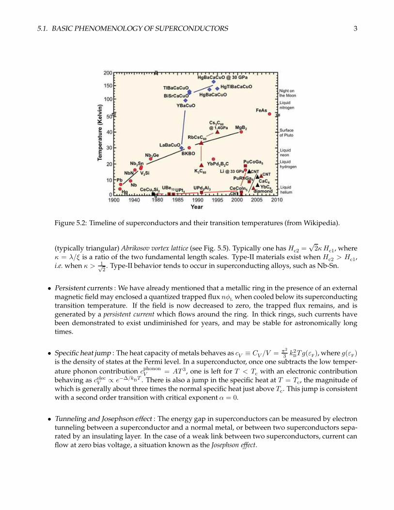
The superconducting state is a phase of matter, as is ferromagnetism, metallicity, etc. The phenomenonwas discovered in the Spring of 1911 by the Dutch physicist H. Kamerlingh Onnes, who observed anabrupt vanishing of the resistivity of solid mercury at T = 4.15K1. Under ambient pressure, there are 33elemental superconductors2, all of which have a metallic phase at higher temperatures, and hundreds ofcompounds and alloys which exhibit the phenomenon. A timeline of superconductors and their criticaltemperatures is provided in Fig. 5.2. The related phenomenon of superfluidity was first discovered inliquid helium below T = 2.17K, at atmospheric pressure, independently in 1937 by P. Kapitza (Moscow)and by J. F. Allen and A. D. Misener (Cambridge). At some level, a superconductor may be consideredas a charged superfluid. Here we recite the basic phenomenology of superconductors:
• Vanishing electrical resistance : The DC electrical resistance at zero magnetic field vanishes inthe superconducting state. This is established in some materials to better than one part in 1015
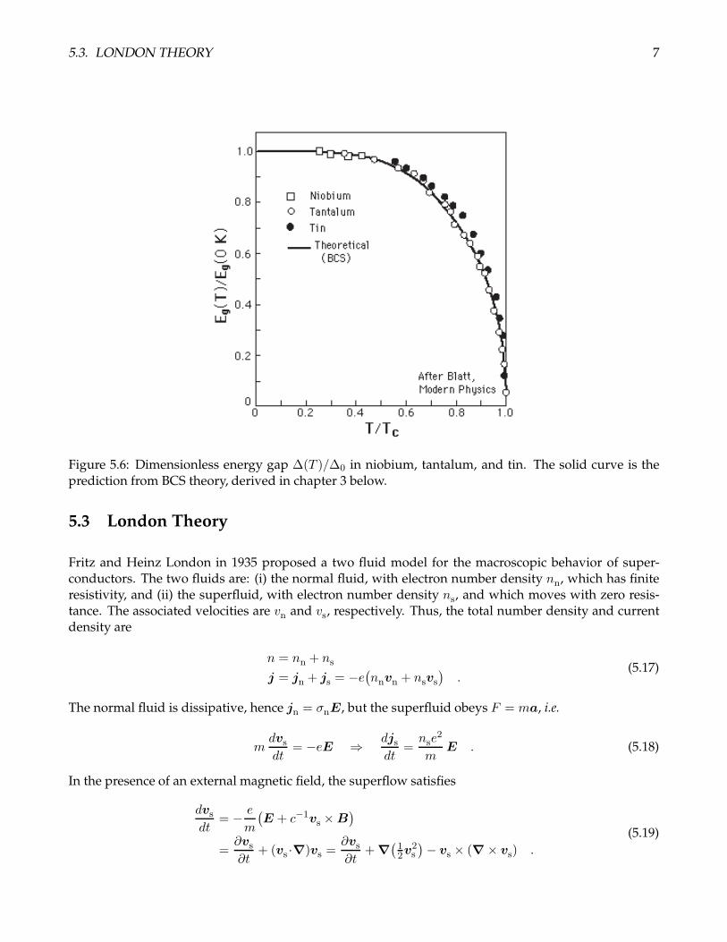
of the normal state resistance. Above the critical temperature Tc, the DC resistivity at H = 0 isfinite. The AC resistivity remains zero up to a critical frequency, ωc = 2∆/~, where ∆ is the gapin the electronic excitation spectrum. The frequency threshold is 2∆ because the superconduct-ing condensate is made up of electron pairs, so breaking a pair results in two quasiparticles, eachwith energy ∆ or greater. For weak coupling superconductors, which are described by the famousBCS theory (1957), there is a relation between the gap energy and the superconducting transitiontemperature, 2∆0 = 3.5 kBTc, which we derive when we study the BCS model. The gap ∆(T ) istemperature-dependent and vanishes at Tc.
• Flux expulsion : In 1933 it was descovered by Meissner and Ochsenfeld that magnetic fields insuperconducting tin and lead to not penetrate into the bulk of a superconductor, but rather areconfined to a surface layer of thickness λ, called the London penetration depth. Typically λ in on thescale of tens to hundreds of nanometers.
1Coincidentally, this just below the temperature at which helium liquefies under atmospheric pressure.2An additional 23 elements are superconducting under high pressure.
1
2 CHAPTER 5. SUPERCONDUCTIVITY
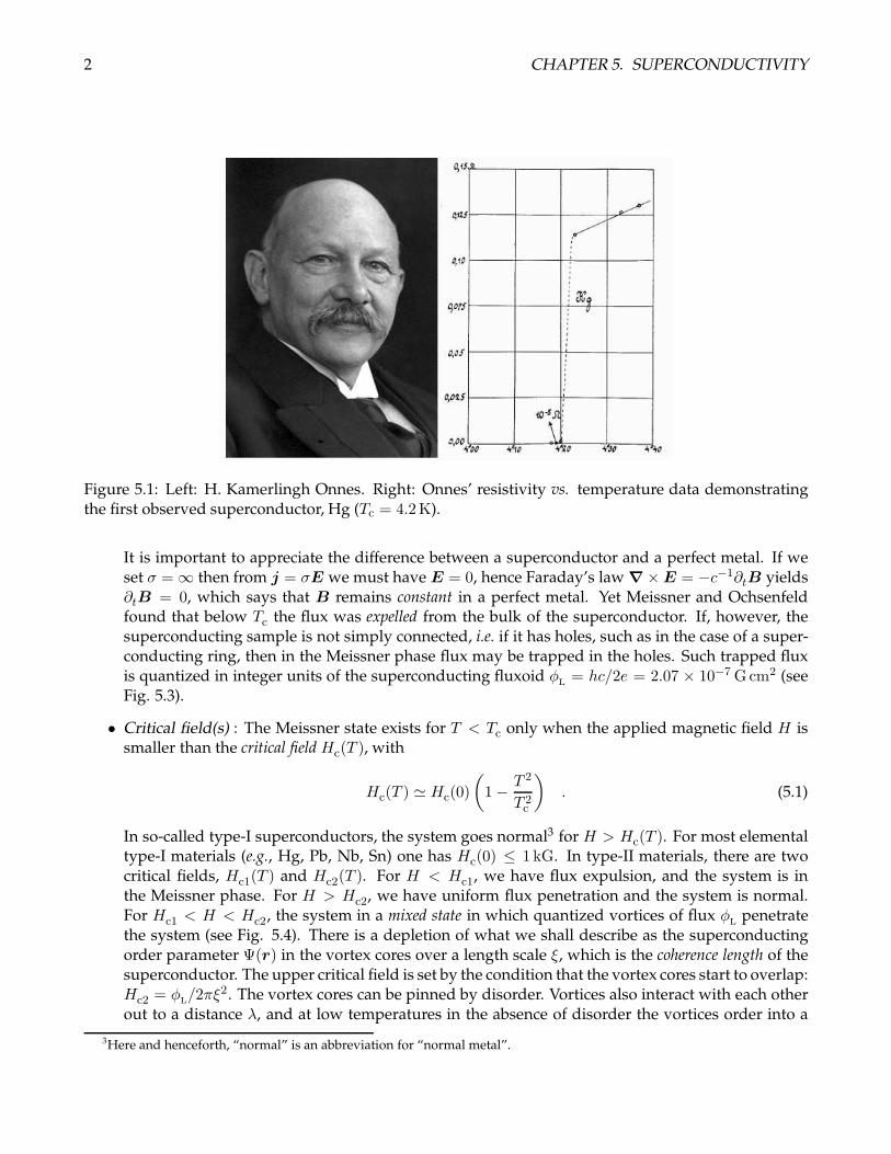
Figure 5.1: Left: H. Kamerlingh Onnes. Right: Onnes’ resistivity vs. temperature data demonstratingthe first observed superconductor, Hg (Tc = 4.2K).
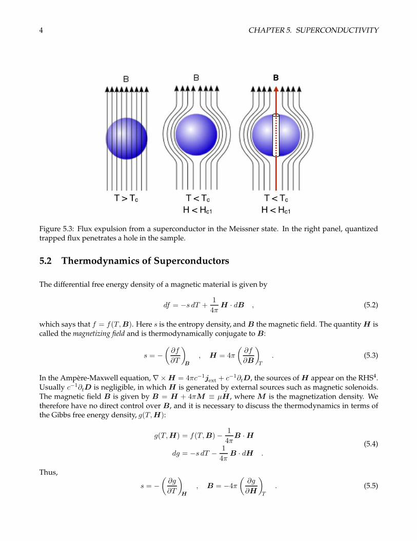
It is important to appreciate the difference between a superconductor and a perfect metal. If weset σ = ∞ then from j = σE we must have E = 0, hence Faraday’s law ∇×E = −c−1∂tB yields∂tB = 0, which says that B remains constant in a perfect metal. Yet Meissner and Ochsenfeldfound that below Tc the flux was expelled from the bulk of the superconductor. If, however, thesuperconducting sample is not simply connected, i.e. if it has holes, such as in the case of a super-conducting ring, then in the Meissner phase flux may be trapped in the holes. Such trapped fluxis quantized in integer units of the superconducting fluxoid φL = hc/2e = 2.07 × 10⁻⁷ Gcm2 (seeFig. 5.3).
• Critical field(s) : The Meissner state exists for T < Tc only when the applied magnetic field H issmaller than the critical field Hc(T ), with
Hc(T ) ≃ Hc(0)
(1− T 2
T 2c
). (5.1)
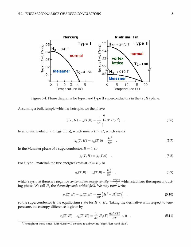
In so-called type-I superconductors, the system goes normal3 for H > Hc(T ). For most elementaltype-I materials (e.g., Hg, Pb, Nb, Sn) one has Hc(0) ≤ 1 kG. In type-II materials, there are twocritical fields, Hc1(T ) and Hc2(T ). For H < Hc1, we have flux expulsion, and the system is inthe Meissner phase. For H > Hc2, we have uniform flux penetration and the system is normal.For Hc1 < H < Hc2, the system in a mixed state in which quantized vortices of flux φL penetratethe system (see Fig. 5.4). There is a depletion of what we shall describe as the superconductingorder parameter Ψ(r) in the vortex cores over a length scale ξ, which is the coherence length of thesuperconductor. The upper critical field is set by the condition that the vortex cores start to overlap:Hc2 = φL/2πξ
2. The vortex cores can be pinned by disorder. Vortices also interact with each otherout to a distance λ, and at low temperatures in the absence of disorder the vortices order into a
3Here and henceforth, “normal” is an abbreviation for “normal metal”.
5.1. BASIC PHENOMENOLOGY OF SUPERCONDUCTORS 3
Figure 5.2: Timeline of superconductors and their transition temperatures (from Wikipedia).
(typically triangular) Abrikosov vortex lattice (see Fig. 5.5). Typically one has Hc2 =√2κHc1, where
κ = λ/ξ is a ratio of the two fundamental length scales. Type-II materials exist when Hc2 > Hc1,i.e. when κ > 1√
2. Type-II behavior tends to occur in superconducting alloys, such as Nb-Sn.
• Persistent currents : We have already mentioned that a metallic ring in the presence of an externalmagnetic field may enclosed a quantized trapped flux nφL when cooled below its superconductingtransition temperature. If the field is now decreased to zero, the trapped flux remains, and isgenerated by a persistent current which flows around the ring. In thick rings, such currents havebeen demonstrated to exist undiminished for years, and may be stable for astronomically longtimes.
• Specific heat jump : The heat capacity of metals behaves as cV ≡ CV /V = π2
3 k2BTg(εF), where g(εF)
is the density of states at the Fermi level. In a superconductor, once one subtracts the low temper-
ature phonon contribution cphononV = AT 3, one is left for T < Tc with an electronic contributionbehaving as celecV ∝ e−∆/kBT . There is also a jump in the specific heat at T = Tc, the magnitude ofwhich is generally about three times the normal specific heat just above Tc. This jump is consistentwith a second order transition with critical exponent α = 0.
• Tunneling and Josephson effect : The energy gap in superconductors can be measured by electrontunneling between a superconductor and a normal metal, or between two superconductors sepa-rated by an insulating layer. In the case of a weak link between two superconductors, current canflow at zero bias voltage, a situation known as the Josephson effect.
4 CHAPTER 5. SUPERCONDUCTIVITY
Figure 5.3: Flux expulsion from a superconductor in the Meissner state. In the right panel, quantizedtrapped flux penetrates a hole in the sample.
5.2 Thermodynamics of Superconductors
The differential free energy density of a magnetic material is given by
df = −s dT +1
4πH · dB , (5.2)
which says that f = f(T,B). Here s is the entropy density, and B the magnetic field. The quantity H iscalled the magnetizing field and is thermodynamically conjugate to B:
s = −(∂f
∂T
)
B
, H = 4π
(∂f
∂B
)
T
. (5.3)
In the Ampere-Maxwell equation, ∇×H = 4πc−1jext + c−1∂tD, the sources of H appear on the RHS4.Usually c−1∂tD is negligible, in which H is generated by external sources such as magnetic solenoids.The magnetic field B is given by B = H + 4πM ≡ µH, where M is the magnetization density. Wetherefore have no direct control over B, and it is necessary to discuss the thermodynamics in terms ofthe Gibbs free energy density, g(T,H):
g(T,H) = f(T,B)− 1
4πB ·H
dg = −s dT − 1
4πB · dH .
(5.4)
Thus,
s = −(∂g
∂T
)
H
, B = −4π
(∂g
∂H
)
T
. (5.5)
5.2. THERMODYNAMICS OF SUPERCONDUCTORS 5
Figure 5.4: Phase diagrams for type I and type II superconductors in the (T,H) plane.
Assuming a bulk sample which is isotropic, we then have
g(T,H) = g(T, 0) − 1
4π
H∫
0
dH ′B(H ′) . (5.6)
In a normal metal, µ ≈ 1 (cgs units), which means B ≈ H , which yields
gn(T,H) = gn(T, 0) −H2
8π. (5.7)
In the Meissner phase of a superconductor,B = 0, so
gs(T,H) = gs(T, 0) . (5.8)
For a type-I material, the free energies cross at H = Hc, so
gs(T, 0) = gn(T, 0)−H2
c
8π, (5.9)
which says that there is a negative condensation energy density −H2c (T )8π which stabilizes the superconduct-
ing phase. We call Hc the thermodynamic critical field. We may now write
gs(T,H)− gn(T,H) =1
8π
(H2 −H2
c (T ))
, (5.10)
so the superconductor is the equilibrium state for H < Hc. Taking the derivative with respect to tem-perature, the entropy difference is given by
ss(T,H)− sn(T,H) =1
4πHc(T )
dHc(T )
dT< 0 , (5.11)
4Throughout these notes, RHS/LHS will be used to abbreviate “right/left hand side”.

6 CHAPTER 5. SUPERCONDUCTIVITY
Figure 5.5: STM image of a vortex lattice in NbSe2 at H = 1T and T = 1.8K. From H. F. Hess et al., Phys.Rev. Lett. 62, 214 (1989).
since Hc(T ) is a decreasing function of temperature. Note that the entropy difference is independent ofthe external magnetizing fieldH . As we see from Fig. 5.4, the derivativeH ′
c(T ) changes discontinuouslyat T = Tc. The latent heat ℓ = T ∆s vanishes because Hc(Tc) itself vanishes, but the specific heat isdiscontinuous:
cs(Tc,H = 0)− cn(Tc,H = 0) =Tc4π
(dHc(T )
dT
)2
Tc
, (5.12)
and from the phenomenological relation of Eqn. 5.1, we have H ′c(Tc) = −2Hc(0)/Tc, hence
∆c ≡ cs(Tc,H = 0)− cn(Tc,H = 0) =H2
c (0)
πTc. (5.13)
We can appeal to Eqn. 5.11 to compute the difference ∆c(T,H) for general T < Tc:
∆c(T,H) =T
8π
d2
dT 2H2
c (T ) . (5.14)
With the approximation of Eqn. 5.1, we obtain
cs(T,H)− cn(T,H) ≃ TH2c (0)
2πT 2c
3
(T
Tc
)2− 1
. (5.15)
In the limit T → 0, we expect cs(T ) to vanish exponentially as e−∆/kBT , hence we have ∆c(T → 0) =−γT , where γ is the coefficient of the linear T term in the metallic specific heat. Thus, we expect γ ≃H2
c (0)/2πT2c . Note also that this also predicts the ratio ∆c(Tc, 0)
/cn(Tc, 0) = 2. In fact, within BCS theory,
this ratio is approximately 1.43. BCS also yields the low temperature form
Hc(T ) = Hc(0)
1− α
(T
Tc
)2+O
(e−∆/kBT
)
(5.16)
with α ≃ 1.07. Thus, HBCSc (0) =
(2πγT 2
c /α)1/2
.
5.3. LONDON THEORY 7
Figure 5.6: Dimensionless energy gap ∆(T )/∆0 in niobium, tantalum, and tin. The solid curve is theprediction from BCS theory, derived in chapter 3 below.
5.3 London Theory
Fritz and Heinz London in 1935 proposed a two fluid model for the macroscopic behavior of super-conductors. The two fluids are: (i) the normal fluid, with electron number density nn, which has finiteresistivity, and (ii) the superfluid, with electron number density ns, and which moves with zero resis-tance. The associated velocities are vn and vs, respectively. Thus, the total number density and currentdensity are
n = nn + ns
j = jn + js = −e(nnvn + nsvs
).
(5.17)
The normal fluid is dissipative, hence jn = σnE, but the superfluid obeys F = ma, i.e.
mdvsdt
= −eE ⇒ djsdt
=nse
2
mE . (5.18)
In the presence of an external magnetic field, the superflow satisfies
dvsdt
= − e
m
(E + c−1vs ×B
)
=∂vs∂t
+ (vs ·∇)vs =∂vs∂t
+∇(12v
2s
)− vs × (∇× vs) .
(5.19)
8 CHAPTER 5. SUPERCONDUCTIVITY
We then have∂vs∂t
+e
mE +∇
(12v
2s
)= vs×
(∇× vs −
eB
mc
). (5.20)
Taking the curl, and invoking Faraday’s law ∇×E = −c−1∂tB, we obtain
∂
∂t
(∇× vs −
eB
mc
)= ∇×
vs ×
(∇× vs −
eB
mc
), (5.21)
which may be written as∂Q
∂t= ∇× (vs ×Q) , (5.22)
where
Q ≡ ∇× vs −eB
mc. (5.23)
Eqn. 5.22 says that if Q = 0, it remains zero for all time. Assumption: the equilibrium state has Q = 0.Thus,
∇× vs =eB
mc⇒ ∇× js = −nse
2
mcB . (5.24)
This equation implies the Meissner effect, for upon taking the curl of the last of Maxwell’s equations(and assuming a steady state so E = D = 0),
−∇2B = ∇× (∇×B) =4π
c∇× j = −4πnse
2
mc2B ⇒ ∇2B = λ−2
L B , (5.25)
where λL =√mc2/4πnse
2 is the London penetration depth. The magnetic field can only penetrate up to adistance on the order of λL inside the superconductor.
Note that∇× js = − c
4πλ2LB (5.26)
and the definition B = ∇×A licenses us to write
js = − c
4πλ2LA , (5.27)
provided an appropriate gauge choice for A is taken. Since ∇ · js = 0 in steady state, we conclude∇ ·A = 0 is the proper gauge. This is called the Coulomb gauge. Note, however, that this still allowsfor the little gauge transformation A → A + ∇χ , provided ∇2χ = 0. Consider now an isolated bodywhich is simply connected, i.e. any closed loop drawn within the body is continuously contractable toa point. The normal component of the superfluid at the boundary, Js,⊥ must vanish, hence A⊥ = 0 aswell. Therefore ∇⊥χ must also vanish everywhere on the boundary, which says that χ is determined upto a global constant.
If the superconductor is multiply connected, though, the condition ∇⊥χ = 0 allows for non-constantsolutions for χ. The line integral of A around a closed loop surrounding a hole D in the superconductoris, by Stokes’ theorem, the magnetic flux through the loop:
∮
∂D
dl ·A =
∫
D
dS n ·B = ΦD . (5.28)

5.4. GINZBURG-LANDAU THEORY 9
On the other hand, within the interior of the superconductor, since B = ∇ × A = 0, we can writeA = ∇χ , which says that the trapped flux ΦD is given by ΦD = ∆χ, then change in the gauge functionas one proceeds counterclockwise around the loop. F. London argued that if the gauge transformationA → A+∇χ is associated with a quantum mechanical wavefunction associated with a charge e object,then the flux ΦD will be quantized in units of the Dirac quantum φ0 = hc/e = 4.137 × 10⁻⁷ Gcm2. Theargument is simple. The transformation of the wavefunction Ψ → Ψ e−iα is cancelled by the replacementA → A + (~c/e)∇α. Thus, we have χ = αφ0/2π, and single-valuedness requires ∆α = 2πn around aloop, hence ΦD = ∆χ = nφ0.
The above argument is almost correct. The final piece was put in place by Lars Onsager in 1953. Onsagerpointed out that if the particles described by the superconducting wavefunction Ψ were of charge e∗ =2e, then, mutatis mutandis, one would conclude the quantization condition is ΦD = nφL, where φL =hc/2e is the London flux quantum, which is half the size of the Dirac flux quantum. This suggestion wasconfirmed in subsequent experiments by Deaver and Fairbank, and by Doll and Nabauer, both in 1961.
De Gennes’ derivation of London Theory
De Gennes writes the total free energy of the superconductor as
F =
∫d3x fs + Ekinetic + Efield
Ekinetic =
∫d3x 1
2mnsv2s (x) =
∫d3x
m
2nse2j2s (x)
Efield =
∫d3x
B2(x)
8π.
(5.29)
But under steady state conditions ∇×B = 4πc−1js, so
F =
∫d3x
fs +
B2
8π+ λ2L
(∇×B)2
8π
. (5.30)
Taking the functional variation and setting it to zero,
4πδF
δB= B + λ2L ∇× (∇×B) = B − λ2L ∇2B = 0 . (5.31)
5.4 Ginzburg-Landau Theory
The basic idea behind Ginzburg-Landau theory is to write the free energy as a simple functional ofthe order parameter(s) of a thermodynamic system and their derivatives. In 4He, the order parameterΨ(x) = 〈ψ(x)〉 is the quantum and thermal average of the field operator ψ(x) which destroys a heliumatom at position x. When Ψ is nonzero, we have Bose condensation with condensate density n0 = |Ψ|2.Above the lambda transition, one has n0(T > Tλ) = 0.

10 CHAPTER 5. SUPERCONDUCTIVITY
In an s-wave superconductor, the order parameter field is given by
Ψ(x) ∝⟨ψ↑(x)ψ↓(x)
⟩, (5.32)
where ψσ(x) destroys a conduction band electron of spin σ at position x. Owing to the anticommutingnature of the fermion operators, the fermion field ψσ(x) itself cannot condense, and it is only the pairfield Ψ(x) (and other products involving an even number of fermion field operators) which can take anonzero value.
5.4.1 Landau theory for superconductors
The superconducting order parameter Ψ(x) is thus a complex scalar, as in a superfluid. As we shall see,the difference is that the superconductor is charged. In the absence of magnetic fields, the Landau freeenergy density is approximated as
f = a |Ψ|2 + 12b |Ψ|4 . (5.33)
The coefficients a and b are real and temperature-dependent but otherwise constant in a spatially homo-geneous system. The sign of a is negotiable, but b > 0 is necessary for thermodynamic stability. The freeenergy has an O(2) symmetry, i.e. it is invariant under the substitution Ψ → Ψ eiα. For a < 0 the freeenergy is minimized by writing
Ψ =
√−abeiφ , (5.34)
where φ, the phase of the superconductor, is a constant. The system spontaneously breaks the O(2)symmetry and chooses a direction in Ψ space in which to point.
In our formulation here, the free energy of the normal state, i.e. when Ψ = 0, is fn = 0 at all temperatures,and that of the superconducting state is fs = −a2/2b. From thermodynamic considerations, therefore,we have
fs(T )− fn(T ) = −H2c (T )
8π⇒ a2(T )
b(T )=H2
c (T )
4π. (5.35)
Furthermore, from London theory we have that λ2L = mc2/4πnse2, and if we normalize the order pa-
rameter according to∣∣Ψ∣∣2 = ns
n, (5.36)
where ns is the number density of superconducting electrons and n the total number density of conduc-tion band electrons, then
λ2L(0)
λ2L(T )=∣∣Ψ(T )
∣∣2 = −a(T )b(T )
. (5.37)
Here we have taken ns(T = 0) = n, so |Ψ(0)|2 = 1. Putting this all together, we find
a(T ) = −H2c (T )
4π· λ
2L(T )
λ2L(0), b(T ) =
H2c (T )
4π· λ
4L(T )
λ4L(0)(5.38)
Close to the transition, Hc(T ) vanishes in proportion to λ−2L (T ), so a(Tc) = 0 while b(Tc) > 0 remains
finite at Tc. Later on below, we shall relate the penetration depth λL to a stiffness parameter in theGinzburg-Landau theory.
5.4. GINZBURG-LANDAU THEORY 11
We may now compute the specific heat discontinuity from c = −T ∂2f∂T 2 . It is left as an exercise to the
reader to show
∆c = cs(Tc)− cn(Tc) =Tc[a′(Tc)
]2
b(Tc), (5.39)
where a′(T ) = da/dT . Of course, cn(T ) isn’t zero! Rather, here we are accounting only for the specificheat due to that part of the free energy associated with the condensate. The Ginzburg-Landau descrip-tion completely ignores the metal, and doesn’t describe the physics of the normal state Fermi surface,which gives rise to cn = γT . The discontinuity ∆c is a mean field result. It works extremely well forsuperconductors, where, as we shall see, the Ginzburg criterion is satisfied down to extremely smalltemperature variations relative to Tc. In 4He, one sees an cusp-like behavior with an apparent weak di-vergence at the lambda transition. Recall that in the language of critical phenomena, c(T ) ∝ |T − Tc|−α.For the O(2) model in d = 3 dimensions, the exponent α is very close to zero, which is close to the meanfield value α = 0. The order parameter exponent is β = 1
2 at the mean field level; the exact value iscloser to 1
3 . One has, for T < Tc,
∣∣Ψ(T < Tc)∣∣ =
√−a(T )b(T )
=
√a′(Tc)b(Tc)
(Tc − T )1/2 + . . . . (5.40)
5.4.2 Ginzburg-Landau Theory
The Landau free energy is minimized by setting |Ψ|2 = −a/b for a < 0. The phase of Ψ is thereforefree to vary, and indeed free to vary independently everywhere in space. Phase fluctuations should costenergy, so we posit an augmented free energy functional,
F[Ψ,Ψ∗] =
∫ddx
a∣∣Ψ(x)
∣∣2 + 12 b∣∣Ψ(x)
∣∣4 +K∣∣∇Ψ(x)
∣∣2 + . . .
. (5.41)
Here K is a stiffness with respect to spatial variation of the order parameter Ψ(x). From K and a, wecan form a length scale, ξ =
√K/|a|, known as the coherence length. This functional in fact is very useful
in discussing properties of neutral superfluids, such as 4He, but superconductors are charged, and wehave instead
F[Ψ,Ψ∗,A
]=
∫ddx
a∣∣Ψ(x)
∣∣2 + 12 b∣∣Ψ(x)
∣∣4 +K∣∣∣(∇+ ie∗
~c A)Ψ(x)
∣∣∣2+ 1
8π (∇×A)2 + . . .
. (5.42)
Here q = −e∗ = −2e is the charge of the condensate. We assume E = 0, so A is not time-dependent.
Under a local transformation Ψ(x) → Ψ(x) eiα(x), we have
(∇+ ie∗
~c A)(Ψ eiα
)= eiα
(∇+ i∇α+ ie∗
~c A)Ψ , (5.43)
which, upon making the gauge transformation A → A − ~ce∗ ∇α, reverts to its original form. Thus, the
free energy is unchanged upon replacing Ψ → Ψeiα and A → A− ~ce∗ ∇α. Since gauge transformations
result in no physical consequences, we conclude that the longitudinal phase fluctuations of a chargedorder parameter do not really exist.

12 CHAPTER 5. SUPERCONDUCTIVITY
5.4.3 Equations of motion
Varying the free energy in Eqn. 5.42 with respect to Ψ∗ and A, respectively, yields
0 =δF
δΨ∗ = aΨ+ b |Ψ|2 Ψ−K(∇+ ie∗
~c A)2
Ψ
0 =δF
δA=
2Ke∗
~c
[1
2i
(Ψ∗
∇Ψ−Ψ∇Ψ∗)+ e∗
~c|Ψ|2A
]+
1
4π∇×B .
(5.44)
The second of these equations is the Ampere-Maxwell law, ∇×B = 4πc−1j, with
j = −2Ke∗
~2
[~
2i
(Ψ∗
∇Ψ−Ψ∇Ψ∗)+ e∗
c|Ψ|2A
]. (5.45)
If we set Ψ to be constant, we obtain ∇× (∇×B) + λ−2L B = 0, with
λ−2L = 8πK
(e∗
~c
)2|Ψ|2 . (5.46)
Thus we recover the relation λ−2L ∝ |Ψ|2. Note that |Ψ|2 = |a|/b in the ordered phase, hence
λ−1L =
[8πa2
b· K|a|
]1/2e∗
~c=
√2 e∗
~cHc ξ , (5.47)
which says
Hc =φL√
8π ξλL
. (5.48)
At a superconductor-vacuum interface, we should have
n ·(~
i∇+
e∗
cA)Ψ∣∣∂Ω
= 0 , (5.49)
where Ω denotes the superconducting region and n the surface normal. This guarantees n · j∣∣∂Ω
= 0,since
j = −2Ke∗
~2Re(~
iΨ∗
∇Ψ+e∗
c|Ψ|2A
). (5.50)
Note that n · j = 0 also holds if
n ·(~
i∇+
e∗
cA)Ψ∣∣∂Ω
= irΨ , (5.51)
with r a real constant. This boundary condition is appropriate at a junction with a normal metal.

5.4. GINZBURG-LANDAU THEORY 13
5.4.4 Critical current
Consider the case where Ψ = Ψ0. The free energy density is
f = a |Ψ0|2 + 12 b |Ψ0|4 +K
(e∗
~c
)2A2 |Ψ0|2 . (5.52)
If a > 0 then f is minimized for Ψ0 = 0. What happens for a < 0, i.e. when T < Tc. Minimizing withrespect to |Ψ0|, we find
|Ψ0|2 =|a| −K(e∗/~c)2A2
b. (5.53)
The current density is then
j = −2cK
(e∗
~c
)2( |a| −K(e∗/~c)2A2
b
)A . (5.54)
Taking the magnitude and extremizing with respect to A = |A| , we obtain the critical current density jc:
A2 =|a|
3K(e∗/~c)2⇒ jc =
4
3√3
cK1/2 |a|3/2b
. (5.55)
Physically, what is happening is this. When the kinetic energy density in the superflow exceeds thecondensation energy density H2
c /8π = a2/2b, the system goes normal. Note that jc(T ) ∝ (Tc − T )3/2.
Should we feel bad about using a gauge-covariant variable like A in the above analysis? Not really,because when we write A, what we really mean is the gauge-invariant combination A + ~c
e∗ ∇ϕ, whereϕ = arg(Ψ) is the phase of the order parameter.
London limit
In the so-called London limit, we write Ψ =√n0 e
iϕ, with n0 constant. Then
j = −2Ke∗n0~
(∇ϕ+
e∗
~cA)= − c
4πλ2L
(φL
2π∇ϕ+A
). (5.56)
Thus,
∇× j =c
4π∇× (∇×B)
= − c
4πλ2LB − c
4πλ2L
φL
2π∇×∇ϕ ,
(5.57)
which says
λ2L ∇2B = B +φL
2π∇×∇ϕ . (5.58)
If we assume B = Bz and the phase field ϕ has singular vortex lines of topological index ni ∈ Z locatedat position ρi in the (x, y) plane, we have
λ2L ∇2B = B + φL
∑
i
ni δ(ρ− ρi
). (5.59)
14 CHAPTER 5. SUPERCONDUCTIVITY
Taking the Fourier transform, we solve for B(q), where k = (q, kz) :
B(q) = − φL
1 + q2λ2L
∑
i
ni e−iq·ρi , (5.60)
whence
B(ρ) = − φL
2πλ2L
∑
i
niK0
( |ρ− ρi|λL
), (5.61)
where K0(z) is the MacDonald function, whose asymptotic behaviors are given by
K0(z) ∼−C− ln(z/2) (z → 0)
(π/2z)1/2 exp(−z) (z → ∞) ,(5.62)
where C = 0.57721566 . . . is the Euler-Mascheroni constant. The logarithmic divergence as ρ → 0 is anartifact of the London limit. Physically, the divergence should be cut off when |ρ − ρi| ∼ ξ. The currentdensity for a single vortex at the origin is
j(r) =nc
4π∇×B = − c
4πλL
· φL
2πλ2LK1
(ρ/λL
)ϕ , (5.63)
where n ∈ Z is the vorticity, and K1(z) = −K ′0(z) behaves as z−1 as z → 0 and exp(−z)/
√2πz as z → ∞.
Note the ith vortex carries magnetic flux ni φL.
5.4.5 Ginzburg criterion
Consider fluctuations in Ψ(x) above Tc. If |Ψ| ≪ 1, we may neglect quartic terms and write
F =
∫ddx
(a |Ψ|2 +K |∇Ψ|2
)=∑
k
(a+Kk2
)|Ψ(k)|2 , (5.64)
where we have expanded
Ψ(x) =1√V
∑
k
Ψ(k) eik·x . (5.65)
The Helmholtz free energy A(T ) is given by
e−A/kBT =
∫D[Ψ,Ψ∗] e−F/T =
∏
k
(πkBT
a+Kk2
), (5.66)
which is to say
A(T ) = kBT∑
k
ln
(πkBT
a+Kk2
). (5.67)
We write a(T ) = αt with t = (T − Tc)/Tc the reduced temperature. We now compute the singularcontribution to the specific heat CV = −TA′′(T ), which only requires we differentiate with respect to T

5.4. GINZBURG-LANDAU THEORY 15
as it appears in a(T ). Dividing by NskB, where Ns = V/ad is the number of lattice sites, we obtain thedimensionless heat capacity per unit cell,
c =α2ad
K2
Λξ∫ddk
(2π)d1
(ξ−2 + k2)2, (5.68)
where Λ ∼ a−1 is an ultraviolet cutoff on the order of the inverse lattice spacing, and ξ = (K/a)1/2 ∝|t|−1/2. We define R∗ ≡ (K/α)1/2, in which case ξ = R∗ |t|−1/2, and
c = R−4∗ ad ξ4−d
Λξ∫ddq
(2π)d1
(1 + q2)2, (5.69)
where q ≡ qξ. Thus,
c(t) ∼
const. if d > 4
− ln t if d = 4
td2−2 if d < 4 .
(5.70)
For d > 4, mean field theory is qualitatively accurate, with finite corrections. In dimensions d ≤ 4, themean field result is overwhelmed by fluctuation contributions as t → 0+ (i.e. as T → T+
c ). We see thatthe Ginzburg-Landau mean field theory is sensible provided the fluctuation contributions are small, i.e.provided
R−4∗ ad ξ4−d ≪ 1 , (5.71)
which entails t≫ tG, where
tG =
(a
R∗
) 2d4−d
(5.72)
is the Ginzburg reduced temperature. The criterion for the sufficiency of mean field theory, namely t≫ tG,is known as the Ginzburg criterion. The region |t| < tG is known as the critical region.
In a lattice ferromagnet, as we have seen, R∗ ∼ a is on the scale of the lattice spacing itself, hence tG ∼ 1and the critical regime is very large. Mean field theory then fails quickly as T → Tc. In a (conventional)three-dimensional superconductor, R∗ is on the order of the Cooper pair size, and R∗/a ∼ 102 − 103,hence tG = (a/R∗)
6 ∼ 10−18 − 10−12 is negligibly narrow. The mean field theory of the superconductingtransition – BCS theory – is then valid essentially all the way to T = Tc.
Another way to think about it is as follows. In dimensions d > 2, for |r| fixed and ξ → ∞, one has5
⟨Ψ∗(r)Ψ(0)
⟩≃ Cd
kBT R2∗
e−r/ξ
rd−2, (5.73)
where Cd is a dimensionless constant. If we compute the ratio of fluctuations to the mean value over a
5Exactly at T = Tc, the correlations behave as⟨
Ψ∗(r)Ψ(0)⟩
∝ r−(d−2+η), where η is a critical exponent.

16 CHAPTER 5. SUPERCONDUCTIVITY
patch of linear dimension ξ, we have
fluctuations
mean=
ξ∫ddr 〈Ψ∗(r)Ψ(0)〉ξ∫ddr 〈|Ψ(r)|2〉
∝ 1
R2∗ ξd |Ψ|2
ξ∫ddr
e−r/ξ
rd−2∝ 1
R2∗ ξd−2 |Ψ|2 .
(5.74)
Close to the critical point we have ξ ∝ R∗ |t|−ν and |Ψ| ∝ |t|β , with ν = 12 and β = 1
2 within mean fieldtheory. Setting the ratio of fluctuations to mean to be small, we recover the Ginzburg criterion.
5.4.6 Domain wall solution
Consider first the simple case of the neutral superfluid. The additional parameter K provides us witha new length scale, ξ =
√K/|a| , which is called the coherence length. Varying the free energy with
respect to Ψ∗(x), one obtains
δF
δΨ∗(x)= aΨ(x) + b
∣∣Ψ(x)∣∣2Ψ(x)−K∇2Ψ(x) . (5.75)
Rescaling, we write Ψ ≡(|a|/b
)1/2ψ, and setting the above functional variation to zero, we obtain
−ξ2∇2ψ + sgn (T − Tc)ψ + |ψ|2ψ = 0 . (5.76)
Consider the case of a domain wall when T < Tc. We assume all spatial variation occurs in the x-direction, and we set ψ(x = 0) = 0 and ψ(x = ∞) = 1. Furthermore, we take ψ(x) = f(x) eiα where α isa constant6. We then have −ξ2f ′′(x)− f + f3 = 0, which may be recast as
ξ2d2f
dx2=
∂
∂f
[14
(1− f2
)2]
. (5.77)
This looks just like F = ma if we regard f as the coordinate, x as time, and −V (f) = 14
(1 − f2
)2. Thus,
the potential describes an inverted double well with symmetric minima at f = ±1. The solution to theequations of motion is then that the ‘particle’ rolls starts at ‘time’ x = −∞ at ‘position’ f = +1 and ‘rolls’down, eventually passing the position f = 0 exactly at time x = 0. Multiplying the above equation byf ′(x) and integrating once, we have
ξ2(df
dx
)2= 1
2
(1− f2
)2+ C , (5.78)
where C is a constant, which is fixed by setting f(x → ∞) = +1, which says f ′(∞) = 0, hence C = 0.Integrating once more,
f(x) = tanh
(x− x0√
2 ξ
), (5.79)
6Remember that for a superconductor, phase fluctuations of the order parameter are nonphysical since they are eliiminableby a gauge transformation.
5.4. GINZBURG-LANDAU THEORY 17
where x0 is the second constant of integration. This, too, may be set to zero upon invoking the boundarycondition f(0) = 0. Thus, the width of the domain wall is ξ(T ). This solution is valid provided that thelocal magnetic field averaged over scales small compared to ξ, i.e. b =
⟨∇×A
⟩, is negligible.
The energy per unit area of the domain wall is given by σ, where
σ =
∞∫
0
dx
K
∣∣∣∣dΨ
dx
∣∣∣∣2
+ a |Ψ|2 + 12 b |Ψ|4
=a2
b
∞∫
0
dx
ξ2(df
dx
)2− f2 + 1
2 f4
.
(5.80)
Now we ask: is domain wall formation energetically favorable in the superconductor? To answer, wecompute the difference in surface energy between the domain wall state and the uniform superconduct-ing state. We call the resulting difference σ, the true domainwall energy relative to the superconductingstate:
σ = σ −∞∫
0
dx
(− H2
c
8π
)
=a2
b
∞∫
0
dx
ξ2(df
dx
)2+ 1
2
(1− f2
)2
≡ H2c
8πδ ,
(5.81)
where we have used H2c = 4πa2/b. Invoking the previous result f ′ = (1 − f2)/
√2 ξ, the parameter δ is
given by
δ = 2
∞∫
0
dx(1− f2
)2= 2
1∫
0
df
(1− f2
)2
f ′=
4√2
3ξ(T ) . (5.82)
Had we permitted a field to penetrate over a distance λL(T ) in the domain wall state, we’d have obtained
δ(T ) =4√2
3ξ(T )− λL(T ) . (5.83)
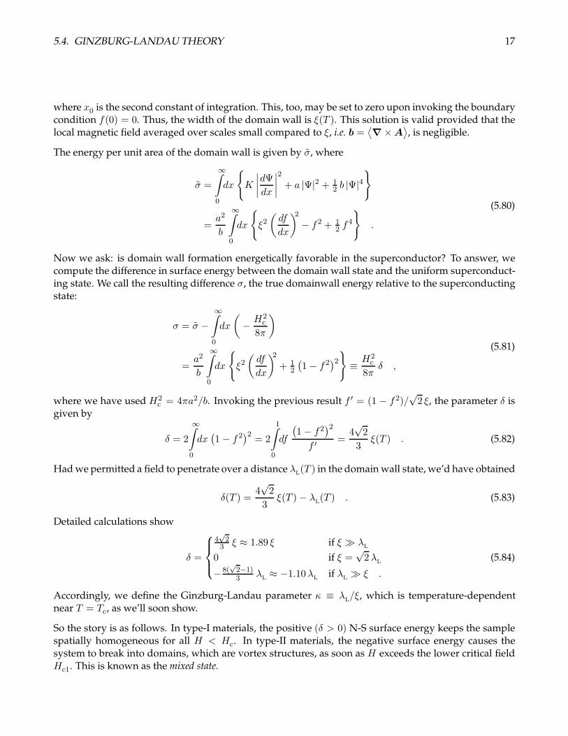
Detailed calculations show
δ =
4√2
3 ξ ≈ 1.89 ξ if ξ ≫ λL
0 if ξ =√2λL
−8(√2−1)3 λL ≈ −1.10λL if λL ≫ ξ .
(5.84)
Accordingly, we define the Ginzburg-Landau parameter κ ≡ λL/ξ, which is temperature-dependentnear T = Tc, as we’ll soon show.
So the story is as follows. In type-I materials, the positive (δ > 0) N-S surface energy keeps the samplespatially homogeneous for all H < Hc. In type-II materials, the negative surface energy causes thesystem to break into domains, which are vortex structures, as soon as H exceeds the lower critical fieldHc1. This is known as the mixed state.

18 CHAPTER 5. SUPERCONDUCTIVITY
5.5 Binding and Dimensionality
Consider a spherically symmetric potential U(r) = −U0 Θ(a − r). Are there bound states, i.e. states inthe eigenspectrum of negative energy? What role does dimension play? It is easy to see that if U0 > 0is large enough, there are always bound states. A trial state completely localized within the well haskinetic energy T0 ≃ ~
2/ma2, while the potential energy is −U0 , so if U0 > ~2/ma2, we have a variational
state with energy E = T0 − U0 < 0, which is of course an upper bound on the true ground state energy.
What happens, though, if U0 < T0? We again appeal to a variational argument. Consider a Gaussian orexponentially localized wavefunction with characteristic size ξ ≡ λa, with λ > 1. The variational energyis then
E ≃ ~2
mξ2− U0
(a
ξ
)d= T0 λ
−2 − U0 λ−d . (5.85)
Extremizing with respect to λ, we obtain −2T0 λ−3 + dU0 λ
−(d+1) and λ =(dU0/2T0
)1/(d−2). Inserting
this into our expression for the energy, we find
E =
(2
d
)2/(d−2)(1− 2
d
)Td/(d−2)0 U
−2/(d−2)0 . (5.86)
We see that for d = 1 we have λ = 2T0/U0 and E = −U20 /4T0 < 0. In d = 2 dimensions, we have
E = (T0 − U0)/λ2, which says E ≥ 0 unless U0 > T0. For weak attractive U(r), the minimum energy
solution is E → 0+, with λ → ∞. It turns out that d = 2 is a marginal dimension, and we shall showthat we always get localized states with a ballistic dispersion and an attractive potential well. For d > 2we have E > 0 which suggests that we cannot have bound states unless U0 > T0, in which case λ ≤ 1and we must appeal to the analysis in the previous paragraph.
We can firm up this analysis a bit by considering the Schrodinger equation,
− ~2
2m∇2ψ(x) + V (x)ψ(x) = E ψ(x) . (5.87)
Fourier transforming, we have
ε(k) ψ(k) +
∫ddk′
(2π)dV (k − k′) ψ(k′) = E ψ(k) , (5.88)
where ε(k) = ~2k2/2m. We may now write V (k − k′) =
∑n λn αn(k)α
∗n(k
′) , which is a decomposition
of the Hermitian matrix Vk,k′ ≡ V (k − k′) into its (real) eigenvalues λn and eigenvectors αn(k). Let’sapproximate Vk,k′ by its leading eigenvalue, which we call λ, and the corresponding eigenvector α(k).
That is, we write Vk,k′ ≃ λα(k)α∗(k′) . We then have
ψ(k) =λα(k)
E − ε(k)
∫ddk′
(2π)dα∗(k′) ψ(k′) . (5.89)
Multiply the above equation by α∗(k) and integrate over k, resulting in
1
λ=
∫ddk
(2π)d
∣∣α(k)∣∣2
E − ε(k)=
1
λ=
∞∫
0
dεg(ε)
E − ε
∣∣α(ε)∣∣2 , (5.90)
5.6. COOPER’S PROBLEM 19
where g(ε) is the density of states g(ε) = Tr δ(ε− ε(k)
). Here, we assume that α(k) = α(k) is isotropic.
It is generally the case that if Vk,k′ is isotropic, i.e. if it is invariant under a simultaneous O(3) rotation
k → Rk and k′ → Rk′, then so will be its lowest eigenvector. Furthermore, since ε = ~2k2/2m is a
function of the scalar k = |k|, this means α(k) can be considered a function of ε. We then have
1
|λ| =∞∫
0
dεg(ε)
|E|+ ε
∣∣α(ε)∣∣2 , (5.91)
where we have we assumed an attractive potential (λ < 0), and, as we are looking for a bound state,E < 0.
If α(0) and g(0) are finite, then in the limit |E| → 0 we have
1
|λ| = g(0) |α(0)|2 ln(1/|E|
)+ finite . (5.92)
This equation may be solved for arbitrarily small |λ| because the RHS of Eqn. 5.91 diverges as |E| → 0.If, on the other hand, g(ε) ∼ εp where p > 0, then the RHS is finite even whenE = 0. In this case, boundstates can only exist for |λ| > λc, where
λc = 1
/ ∞∫
0
dεg(ε)
ε
∣∣α(ε)∣∣2 . (5.93)
Typically the integral has a finite upper limit, given by the bandwidth B. For the ballistic dispersion,one has g(ε) ∝ ε(d−2)/2, so d = 2 is the marginal dimension. In dimensions d ≤ 2, bound states form forarbitrarily weak attractive potentials.
5.6 Cooper’s Problem
In 1956, Leon Cooper considered the problem of two electrons interacting in the presence of a quiescentFermi sea. The background electrons comprising the Fermi sea enter the problem only through theirPauli blocking. Since spin and total momentum are conserved, Cooper first considered a zero momentumsinglet,
|Ψ 〉 =∑
k
Ak
(c†k↑c
†−k↓ − c†k↓c
†−k↑)|F 〉 , (5.94)
where |F 〉 is the filled Fermi sea, |F 〉 =∏
|p|<kFc†p↑c
†p↓ | 0 〉 . Only states with k > kF contribute to the RHS
of Eqn. 5.94, due to Pauli blocking. The real space wavefunction is
Ψ(r1, r2) =∑
k
Ak eik·(r1−r2)
(|↑1↓2 〉 − |↓1↑2 〉
), (5.95)
with Ak = A−k to enforce symmetry of the orbital part. It should be emphasized that this is a two-particle wavefunction, and not an (N +2)-particle wavefunction, with N the number of electrons in the

20 CHAPTER 5. SUPERCONDUCTIVITY
Fermi sea. Again, the Fermi sea in this analysis has no dynamics of its own. Its presence is reflected onlyin the restriction k > kF for the states which participate in the Cooper pair.
The many-body Hamiltonian is written
H =∑
kσ
εk c†kσckσ + 1
2
∑
k1σ1
∑
k2σ2
∑
k3σ3
∑
k4σ4
〈k1σ1,k2σ2 | v |k3σ3,k4σ4 〉 c†k1σ1c†k2σ2
ck4σ4ck3σ3
. (5.96)
We treat |Ψ 〉 as a variational state, which means we set
δ
δA∗k
〈Ψ | H |Ψ 〉〈Ψ |Ψ 〉 = 0 , (5.97)
resulting in
(E − E0)Ak = 2εk Ak +∑
k′
Vk,k′ Ak′ , (5.98)
where
Vk,k′ = 〈k↑,−k↓ | v |k′ ↑,−k′ ↓ 〉 = 1
V
∫d3r v(r) ei(k−k′)·r . (5.99)
Here E0 = 〈F | H |F 〉 is the energy of the Fermi sea.
We write εk = εF + ξk, and we define E ≡ E0 + 2εF +W . Then
W Ak = 2ξk Ak +∑
k′
Vk,k′ Ak′ . (5.100)
If Vk,k′ is rotationally invariant, meaning it is left unchanged by k → Rk and k′ → Rk′ where R ∈ O(3),then we may write
Vk,k′ =
∞∑
ℓ=0
ℓ∑
m=−ℓ
Vℓ(k, k′)Y ℓ
m(k)Y ℓ−m(k′) . (5.101)
We assume that Vl(k, k′) is separable, meaning we can write
Vℓ(k, k′) =
1
Vλℓ αℓ(k)α
∗ℓ (k
′) . (5.102)
This simplifies matters and affords us an exact solution, for now we take Ak = Ak Yℓm(k) to obtain a
solution in the ℓ angular momentum channel:
WℓAk = 2ξk Ak + λℓ αℓ(k) ·1
V
∑
k′
α∗ℓ (k
′)Ak′ , (5.103)
which may be recast as
Ak =λℓ αℓ(k)
Wℓ − 2ξk· 1
V
∑
k′
α∗ℓ (k
′)Ak′ . (5.104)
Now multiply by α∗k and sum over k to obtain
1
λℓ=
1
V
∑
k
∣∣αℓ(k)∣∣2
Wℓ − 2ξk≡ Φ(Wℓ) . (5.105)

5.6. COOPER’S PROBLEM 21
Figure 5.7: Graphical solution to the Cooper problem. A bound state exists for arbitrarily weak λ < 0.
We solve this for Wℓ.
We may find a graphical solution. Recall that the sum is restricted to k > kF, and that ξk ≥ 0. Thedenominator on the RHS of Eqn. 5.105 changes sign as a function of Wℓ every time 1
2Wℓ passes throughone of the ξk values7. A sketch of the graphical solution is provided in Fig. 5.7. One sees that if λℓ < 0,i.e. if the potential is attractive, then a bound state exists. This is true for arbitrarily weak |λℓ|, a situationnot usually encountered in three-dimensional problems, where there is usually a critical strength of theattractive potential in order to form a bound state8. This is a density of states effect – by restricting ourattention to electrons near the Fermi level, where the DOS is roughly constant at g(εF) = m∗kF/π
2~2,
rather than near k = 0, where g(ε) vanishes as√ε, the pairing problem is effectively rendered two-
dimensional. We can make further progress by assuming a particular form for αℓ(k):
αℓ(k) =
1 if 0 < ξk < Bℓ
0 otherwise ,(5.106)
where Bℓ is an effective bandwidth for the ℓ channel. Then
1 = 12 |λℓ|
Bℓ∫
0
dξg(εF + ξ)∣∣Wℓ
∣∣+ 2ξ. (5.107)
The factor of 12 is because it is the DOS per spin here, and not the total DOS. We assume g(ε) does not
vary significantly in the vicinity of ε = εF, and pull g(εF) out from the integrand. Integrating and solvingfor∣∣Wℓ
∣∣,∣∣Wℓ
∣∣ = 2Bℓ
exp(
4|λℓ| g(εF)
)− 1
. (5.108)
7We imagine quantizing in a finite volume, so the allowed k values are discrete.8For example, the 2He molecule is unbound, despite the attractive −1/r6 van der Waals attractive tail in the interatomic
potential.

22 CHAPTER 5. SUPERCONDUCTIVITY
In the weak coupling limit, where |λℓ| g(εF) ≪ 1, we have
∣∣Wℓ
∣∣ ≃ 2Bℓ exp
(− 4
|λℓ| g(εF)
). (5.109)
As we shall see when we study BCS theory, the factor in the exponent is twice too large. The coefficient2Bℓ will be shown to be the Debye energy of the phonons; we will see that it is only over a narrowrange of energies about the Fermi surface that the effective electron-electron interaction is attractive. Forstrong coupling,
|Wℓ| = 12 |λℓ| g(εF) . (5.110)
Finite momentum Cooper pair
We can construct a finite momentum Cooper pair as follows:
|Ψq 〉 =∑
k
Ak
(c†k+ 1
2q ↑c
†−k+ 1
2q ↓ − c†
k+ 12q ↓c
†−k+ 1
2q ↑)|F 〉 . (5.111)
This wavefunction is a momentum eigenstate, with total momentum P = ~q. The eigenvalue equationis then
WAk =(ξk+ 1
2q+ ξ−k+ 1
2q
)Ak +
∑
k′
Vk,k′ Ak′ . (5.112)
Assuming ξk = ξ−k ,
ξk+ 1
2q+ ξ−k+ 1
2q= 2 ξk + 1
4 qαqβ
∂2ξk∂kα ∂kβ
+ . . . . (5.113)
The binding energy is thus reduced by an amount proportional to q2 ; the q = 0 Cooper pair has thegreatest binding energy9.
Mean square radius of the Cooper pair
We have
⟨r2⟩=
∫d3r∣∣Ψ(r)
∣∣2 r2∫d3r∣∣Ψ(r)
∣∣2 =
∫d3k∣∣∇kAk
∣∣2∫d3k∣∣Ak
∣∣2
≃g(εF) ξ
′(kF)2∞∫0
dξ∣∣∂A∂ξ
∣∣2
g(εF)∞∫0
dξ |A|2
(5.114)
9We assume the matrix ∂α∂β ξk is positive definite.
5.7. REDUCED BCS HAMILTONIAN 23
with A(ξ) = −C/(|W |+ 2ξ
)and thus A′(ξ) = 2C/
(|W |+ 2ξ
)2, where C is a constant independent of ξ.
Ignoring the upper cutoff on ξ at Bℓ, we have
⟨r2⟩= 4 ξ′(kF)
2 ·
∞∫
|W |du u−4
∞∫
|W |du u−2
= 43 (~vF)
2 |W |−2 , (5.115)
where we have used ξ′(kF) = ~vF. Thus, RRMS = 2~vF/√
3 |W | . In the weak coupling limit, where |W |is exponentially small in 1/|λ|, the Cooper pair radius is huge. Indeed it is so large that many otherCooper pairs have their centers of mass within the radius of any given pair. This feature is what makesthe BCS mean field theory of superconductivity so successful. Recall in our discussion of the Ginzburgcriterion in §1.4.5, we found that mean field theory was qualitatively correct down to the Ginzburgreduced temperature tG = (a/R∗)
2d/(4−d), i.e. tG = (a/R∗)6 for d = 3. In this expression, R∗ should be
the mean Cooper pair size, and a a microscopic length (i.e. lattice constant). Typically R∗/a ∼ 102 − 103,so tG is very tiny indeed.
5.7 Reduced BCS Hamiltonian
The operator which creates a Cooper pair with total momentum q is b†k,q + b†−k,q , where
b†k,q = c†k+ 1
2q ↑ c
†−k+ 1
2q ↓ (5.116)
is a composite operator which creates the state |k + 12q ↑ , −k + 1
2q ↓ 〉. We learned from the solution tothe Cooper problem that the q = 0 pairs have the greatest binding energy. This motivates considerationof the so-called reduced BCS Hamiltonian,
Hred =∑
k,σ
εk c†kσ ckσ +
∑
k,k′
Vk,k′ b†k,0 bk′,0 . (5.117)
The most general form for a momentum-conserving interaction is
V =1
2V
∑
k,p,q
∑
σ,σ′
uσσ′(k,p, q) c†k+q σ c
†p−q σ′ cp σ′ ck σ . (5.118)
Taking p = −k, σ′ = −σ, and defining k′ ≡ k + q , we have
V → 1
2V
∑
k,k′,σ
v(k,k′) c†k′σ c†−k′ −σ c−k−σ ckσ , (5.119)
where v(k,k′) = u↑↓(k,−k,k′ − k), which is equivalent to Hred .
If Vk,k′ is attractive, then the ground state will have no pair (k ↑ , −k ↓) occupied by a single electron;the pair states are either empty or doubly occupied. In that case, the reduced BCS Hamiltonian may be
24 CHAPTER 5. SUPERCONDUCTIVITY
Figure 5.8: John Bardeen, Leon Cooper, and J. Robert Schrieffer.
written as10
H0red =
∑
k
2εk b†k,0 bk,0 +
∑
k,k′
Vk,k′ b†k,0 bk′,0 . (5.120)
This has the innocent appearance of a noninteracting bosonic Hamiltonian – an exchange of Cooperpairs restores the many-body wavefunction without a sign change because the Cooper pair is a com-posite object consisting of an even number of fermions11. However, this is not quite correct, because the
operators bk,0 and bk′,0 do not satisfy canonical bosonic commutation relations. Rather,
[bk,0 , bk′,0
]=[b†k,0 , b
†k′,0
]= 0
[bk,0 , b
†k′,0
]=(1− c†k↑ck↑ − c†−k↓c−k↓
)δkk′ .
(5.121)
Because of this, H0red cannot naıvely be diagonalized. The extra terms inside the round brackets on the
RHS arise due to the Pauli blocking effects. Indeed, one has (b†k,0)2 = 0, so b†k,0 is no ordinary boson
operator.
Suppose, though, we try a mean field Hartree-Fock approach. We write
bk,0 = 〈bk,0〉+
δbk,0︷ ︸︸ ︷(
bk,0 − 〈bk,0〉)
, (5.122)
and we neglect terms in Hred proportional to δb†k,0 δbk′,0. We have
Hred =∑
k,σ
εk c†kσ ckσ +
∑
k,k′
Vk,k′
(energy shift︷ ︸︸ ︷
−〈b†k,0〉 〈bk′,0〉 +
keep this︷ ︸︸ ︷〈bk′,0〉 b
†k,0 + 〈b†k,0〉 bk′,0 +
drop this!︷ ︸︸ ︷δb†k,0 δbk′,0
). (5.123)
10Spin rotation invariance and a singlet Cooper pair requires that Vk,k′= Vk,−k′
= V−k,k′
.11Recall that the atom 4He, which consists of six fermions (two protons, two neutrons, and two electrons), is a boson, while
3He, which has only one neutron and thus five fermions, is itself a fermion.
5.8. SOLUTION OF THE MEAN FIELD HAMILTONIAN 25
Dropping the last term, which is quadratic in fluctuations, we obtain
HMFred =
∑
k,σ
εk c†kσ ckσ +
∑
k
(∆k c
†k↑ c
†−k↓ +∆∗
k c−k↓ ck↑)−∑
k,k′
Vk,k′ 〈b†k,0〉 〈bk′,0〉 , (5.124)
where
∆k =∑
k′
Vk,k′
⟨c−k′↓ ck′↑
⟩, ∆∗
k =∑
k′
V ∗k,k′
⟨c†k′↑ c
†−k′↓
⟩. (5.125)
The first thing to notice about HMFred is that it does not preserve particle number, i.e. it does not commute
with N =∑
k,σ c†kσckσ. Accordingly, we are practically forced to work in the grand canonical ensemble,
and we define the grand canonical Hamiltonian K ≡ H − µN .
5.8 Solution of the mean field Hamiltonian
We now subtract µN from Eqn. 5.124, and define KBCS ≡ HMFred − µN . Thus,
KBCS =∑
k
(c†k↑ c−k↓
)K
k︷ ︸︸ ︷(ξk ∆k
∆∗k −ξk
) (ck↑c†−k↓
)+K0 , (5.126)
with ξk = εk − µ, and where
K0 =∑
k
ξk −∑
k,k′
Vk,k′ 〈c†k↑c†−k↓〉 〈c−k′↓ ck′↑〉 (5.127)
is a constant. This problem may be brought to diagonal form via a unitary transformation,
(ck↑c†−k↓
)=
Uk︷ ︸︸ ︷(
cos ϑk − sinϑk eiφ
k
sinϑk e−iφ
k cos ϑk
) (γk↑γ†−k↓
). (5.128)
In order for the γkσ operators to satisfy fermionic anticommutation relations, the matrix Uk must beunitary12. We then have
ckσ = cos ϑk γkσ − σ sinϑk eiφ
k γ†−k−σ
γkσ = cos ϑk ckσ + σ sinϑk eiφ
k c†−k−σ .(5.129)
EXERCISE: Verify thatγkσ , γ
†k′σ′
= δkk′ δσσ′ .
12The most general 2× 2 unitary matrix is of the above form, but with each row multiplied by an independent phase. Thesephases may be absorbed into the definitions of the fermion operators themselves. After absorbing these harmless phases, wehave written the most general unitary transformation.
26 CHAPTER 5. SUPERCONDUCTIVITY
We now must compute the transformed Hamiltonian. Dropping the k subscript for notational conve-nience, we have
K = U †KU =
(cos ϑ sinϑ eiφ
− sinϑ e−iφ cos ϑ
)(ξ ∆∆∗ −ξ
)(cos ϑ − sinϑ eiφ
sinϑ e−iφ cos ϑ
)(5.130)
=
((cos2ϑ− sin2ϑ) ξ + sinϑ cos ϑ (∆ e−iφ +∆∗eiφ) ∆ cos2ϑ−∆∗e2iφ sin2ϑ− 2ξ sinϑ cos ϑ eiφ
∆∗ cos2ϑ−∆e−2iφ sin2ϑ− 2ξ sinϑ cos ϑ e−iφ (sin2ϑ− cos2ϑ) ξ − sinϑ cos ϑ (∆ e−iφ +∆∗eiφ)
).
We now use our freedom to choose ϑ and φ to render K diagonal. That is, we demand φ = arg(∆) and
2ξ sinϑ cos ϑ = ∆(cos2ϑ− sin2ϑ) . (5.131)
This says tan(2ϑ) = ∆/ξ, which means
cos(2ϑ) =ξ
E, sin(2ϑ) =
∆
E, E =
√ξ2 +∆2 . (5.132)
The upper left element of K then becomes
(cos2ϑ− sin2ϑ) ξ + sinϑ cos ϑ (∆ e−iφ +∆∗eiφ) =ξ2
E+
∆2
E= E , (5.133)
and thus K =
(E 00 −E
). This unitary transformation, which mixes particle and hole states, is called a
Bogoliubov transformation, because it was first discovered by Valatin.
Restoring the k subscript, we have φk = arg(∆k), and tan(2ϑk) = |∆k|/ξk, which means
cos(2ϑk) =ξkEk
, sin(2ϑk) =|∆k|Ek
, Ek =√ξ2k + |∆k|2 . (5.134)
Assuming that ∆k is not strongly momentum-dependent, we see that the dispersionEk of the excitationshas a nonzero minimum at ξk = 0, i.e. at k = kF. This minimum value of Ek is called the superconductingenergy gap.
We may further write
cos ϑk =
√Ek + ξk2Ek
, sinϑk =
√Ek − ξk2Ek
. (5.135)
The grand canonical BCS Hamiltonian then becomes
KBCS =∑
k,σ
Ek γ†kσ γkσ +
∑
k
(ξk − Ek)−∑
k,k′
Vk,k′ 〈c†k↑c†−k↓〉 〈c−k′↓ ck′↑〉 . (5.136)
Finally, what of the ground state wavefunction itself? We must have γkσ |G 〉 = 0. This leads to
|G 〉 =∏
k
(cos ϑk − sinϑk e
iφk c†k↑ c
†−k↓)| 0 〉 . (5.137)
Note that 〈G |G 〉 = 1. J. R. Schrieffer conceived of this wavefunction during a subway ride in New YorkCity sometime during the winter of 1957. At the time he was a graduate student at the University ofIllinois.
5.9. SELF-CONSISTENCY 27
Sanity check
It is good to make contact with something familiar, such as the case ∆k = 0. Note that ξk < 0 for k < kF
and ξk > 0 for k > kF . We now have
cos ϑk = Θ(k − kF) , sinϑk = Θ(kF − k) . (5.138)
Note that the wavefunction |G 〉 in Eqn. 5.137 correctly describes a filled Fermi sphere out to k = kF.Furthermore, the constant on the RHS of Eqn. 5.136 is 2
∑k<kF
ξk, which is the Landau free energy of
the filled Fermi sphere. What of the excitations? We are free to take φk = 0. Then
k < kF : γ†kσ = σ c−k−σ
k > kF : γ†kσ = c†kσ .(5.139)
Thus, the elementary excitations are holes below kF and electrons above kF. All we have done, then, isto effect a (unitary) particle-hole transformation on those states lying within the Fermi sea.
5.9 Self-consistency
We now demand that the following two conditions hold:
N =∑
kσ
〈c†kσ ckσ〉
∆k =∑
k′
Vk,k′ 〈c−k′↓ ck′↑〉 ,(5.140)
the second of which is from Eqn. 5.125. Thus, we need
〈c†kσ ckσ〉 =⟨(cos ϑk γ
†kσ − σ sinϑk e
−iφk γ−k−σ)(cos ϑk γkσ − σ sinϑk e
iφk γ†−k−σ)
⟩
= cos2ϑk fk + sin2ϑk (1− fk) =1
2− ξk
2Ek
tanh(12βEk
),
(5.141)
where
fk = 〈γ†kσ γkσ〉 =1
eβEk + 1= 1
2 − 12 tanh
(12βEk
)(5.142)
is the Fermi function, with β = 1/kBT . We also have
〈c−k−σ ckσ〉 =⟨(cos ϑk γ−k−σ + σ sinϑk e
iφk γ†kσ)(cos ϑk γkσ − σ sinϑk e
iφk γ†−k−σ)
⟩
= σ sinϑk cos ϑk eiφ
k(2fk − 1
)= −σ∆k
2Ek
tanh(12βEk
).
(5.143)
Let’s evaluate at T = 0 :
N =∑
k
(1− ξk
Ek
)
∆k = −∑
k′
Vk,k′
∆k′
2Ek′
.
(5.144)
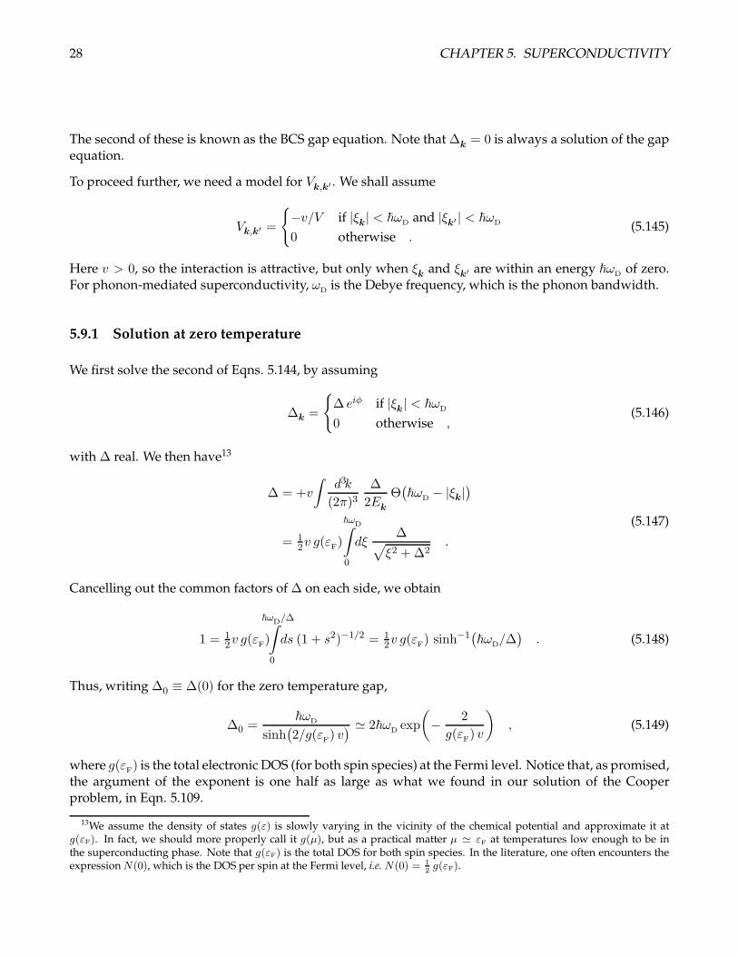
28 CHAPTER 5. SUPERCONDUCTIVITY
The second of these is known as the BCS gap equation. Note that ∆k = 0 is always a solution of the gapequation.
To proceed further, we need a model for Vk,k′ . We shall assume
Vk,k′ =
−v/V if |ξk| < ~ωD and |ξk′ | < ~ωD
0 otherwise .(5.145)
Here v > 0, so the interaction is attractive, but only when ξk and ξk′ are within an energy ~ωD of zero.For phonon-mediated superconductivity, ωD is the Debye frequency, which is the phonon bandwidth.
5.9.1 Solution at zero temperature
We first solve the second of Eqns. 5.144, by assuming
∆k =
∆ eiφ if |ξk| < ~ωD
0 otherwise ,(5.146)
with ∆ real. We then have13
∆ = +v
∫d3k
(2π)3∆
2Ek
Θ(~ωD − |ξk|
)
= 12v g(εF)
~ωD∫
0
dξ∆√
ξ2 +∆2.
(5.147)
Cancelling out the common factors of ∆ on each side, we obtain
1 = 12v g(εF)
~ωD/∆∫
0
ds (1 + s2)−1/2 = 12v g(εF) sinh
−1(~ωD/∆
). (5.148)
Thus, writing ∆0 ≡ ∆(0) for the zero temperature gap,
∆0 =~ωD
sinh(2/g(εF) v
) ≃ 2~ωD exp
(− 2
g(εF) v
), (5.149)
where g(εF) is the total electronic DOS (for both spin species) at the Fermi level. Notice that, as promised,the argument of the exponent is one half as large as what we found in our solution of the Cooperproblem, in Eqn. 5.109.
13We assume the density of states g(ε) is slowly varying in the vicinity of the chemical potential and approximate it atg(εF). In fact, we should more properly call it g(µ), but as a practical matter µ ≃ εF at temperatures low enough to be inthe superconducting phase. Note that g(εF) is the total DOS for both spin species. In the literature, one often encounters theexpression N(0), which is the DOS per spin at the Fermi level, i.e. N(0) = 1
2g(εF).

5.10. COHERENCE FACTORS AND QUASIPARTICLE ENERGIES 29
5.9.2 Condensation energy
We now evaluate the zero temperature expectation of KBCS from Eqn. 5.136. To get the correct answer, itis essential that we retain the term corresponding to the constant energy shift in the mean field Hamil-
tonian, i.e. the last term on the RHS of Eqn. 5.136. Invoking the gap equation ∆k =∑
k′ Vk,k′ 〈c−k′↓ ck′↑〉,we have
〈G | KBCS |G 〉 =∑
k
(ξk − Ek +
|∆k|22Ek
). (5.150)
From this we subtract the ground state energy of the metallic phase, i.e. when ∆k = 0, which is2∑
k ξk Θ(kF − k). The difference is the condensation energy. Adopting the model interaction potentialin Eqn. 5.145, we have
Es − En =∑
k
(ξk −Ek +
|∆k|22Ek
− 2ξk Θ(kF − k)
)
= 2∑
k
(ξk − Ek)Θ(ξk)Θ(~ωD − ξk) +
∑
k
∆20
2Ek
Θ(~ωD − |ξk|
),
(5.151)
where we have linearized about k = kF. We then have
Es − En = V g(εF)∆20
~ωD/∆0∫
0
ds
(s−
√s2 + 1 +
1
2√s2 + 1
)
= 12 V g(εF)∆
20
(x2 − x
√1 + x2
)≈ −1
4 V g(εF)∆20 ,
(5.152)
where x ≡ ~ωD/∆0. The condensation energy density is therefore −14 g(εF)∆
20, which may be equated
with −H2c /8π, where Hc is the thermodynamic critical field. Thus, we find
Hc(0) =√
2πg(εF) ∆0 , (5.153)
which relates the thermodynamic critical field to the superconducting gap, at T = 0.
5.10 Coherence factors and quasiparticle energies
When ∆k = 0, we have Ek = |ξk|. When ~ωD ≪ εF, there is a very narrow window surroundingk = kF where Ek departs from |ξk|, as shown in the bottom panel of Fig. 5.9. Note the energy gap in thequasiparticle dispersion, where the minimum excitation energy is given by14
minkEk = EkF
= ∆0 . (5.154)
In the top panel of Fig. 5.9 we plot the coherence factors sin2ϑk and cos2ϑk. Note that sin2ϑk approachesunity for k < kF and cos2ϑk approaches unity for k > kF, aside for the narrow window of width δk ≃∆0/~vF . Recall that
γ†kσ = cos ϑk c†kσ + σ sinϑk e
−iφk c−k−σ . (5.155)
14Here we assume, without loss of generality, that ∆ is real.

30 CHAPTER 5. SUPERCONDUCTIVITY
Figure 5.9: Top panel: BCS coherence factors sin2ϑk (blue) and cos2ϑk (red). Bottom panel: the functionsξk (black) and Ek (magenta). The minimum value of the magenta curve is the superconducting gap ∆0.
Thus we see that the quasiparticle creation operator γ†kσ creates an electron in the state |k σ 〉 whencos2ϑk ≃ 1, and a hole in the state | −k −σ 〉 when sin2ϑk ≃ 1. In the aforementioned narrow window
|k − kF|<∼∆0/~vF , the quasiparticle creates a linear combination of electron and hole states. Typically∆0 ∼ 10−4 εF, since metallic Fermi energies are on the order of tens of thousands of Kelvins, while ∆0 ison the order of Kelvins or tens of Kelvins. Thus, δk <∼ 10−3kF. The difference between the superconduct-ing state and the metallic state all takes place within an onion skin at the Fermi surface!
Note that for the model interaction Vk,k′ of Eqn. 5.145, the solution ∆k in Eqn. 5.146 is actually discon-
tinuous when ξk = ±~ωD , i.e. when k = k∗± ≡ kF ± ωD/vF. Therefore, the energy dispersion Ek is alsodiscontinuous along these surfaces. However, the magnitude of the discontinuity is
δE =√
(~ωD)2 +∆2
0 − ~ωD ≈ ∆20
2~ωD
. (5.156)
Therefore δE/Ek∗±
≈ ∆20
/2(~ωD)
2 ∝ exp(− 4/g(εF) v
), which is very tiny in weak coupling, where
g(εF) v ≪ 1. Note that the ground state is largely unaffected for electronic states in the vicinity of this(unphysical) energy discontinuity. The coherence factors are distinguished from those of a Fermi liquid
only in regions where 〈c†k↑c†−k↓〉 is appreciable, which requires ξk to be on the order of ∆k. This only
happens when |k−kF|<∼∆0/~vF , as discussed in the previous paragraph. In a more physical model, the

5.11. NUMBER AND PHASE 31
interaction Vk,k′ and the solution ∆k would not be discontinuous functions of k.
5.11 Number and Phase
The BCS ground state wavefunction |G 〉 was given in Eqn. 5.137. Consider the state
|G(α) 〉 =∏
k
(cos ϑk − eiα eiφk sinϑk c
†k↑ c
†−k↓)| 0 〉 . (5.157)
This is the ground state when the gap function ∆k is multiplied by the uniform phase factor eiα. Weshall here abbreviate |α 〉 ≡ |G(α) 〉.
Now consider the action of the number operator on |α 〉 :
N |α 〉 =∑
k
(c†k↑ck↑ + c†−k↓c−k↓
)|α 〉 (5.158)
= −2∑
k
eiα eiφk sinϑk c†k↑ c
†−k↓
∏
k′ 6=k
(cos ϑk′ − eiα eiφk′ sinϑk′ c
†k′↑ c
†−k′↓
)| 0 〉
=2
i
∂
∂α|α 〉 .
If we define the number of Cooper pairs as M ≡ 12N , then we may identify M = 1
i∂∂α . Furthermore, we
may project |G 〉 onto a state of definite particle number by defining
|M 〉 =π∫
−π
dα
2πe−iMα |α 〉 . (5.159)
The state |M 〉 has N = 2M particles, i.e. M Cooper pairs. One can easily compute the number fluctua-tions in the state |G(α) 〉 :
〈α | N2 |α 〉 − 〈α | N |α 〉2
〈α | N |α 〉=
2∫d3k sin2ϑk cos2ϑk∫d3k sin2ϑk
. (5.160)
Thus, (∆N)RMS ∝√
〈N〉. Note that (∆N)RMS vanishes in the Fermi liquid state, where sinϑk cos ϑk = 0.
5.12 Finite temperature
The gap equation at finite temperature takes the form
∆k = −∑
k′
Vk,k′
∆k′
2Ek′
tanh
(Ek′
2kBT
). (5.161)
32 CHAPTER 5. SUPERCONDUCTIVITY
It is easy to see that we have no solutions other than the trivial one ∆k = 0 in the T → ∞ limit, for thegap equation then becomes
∑k′ Vk,k′ ∆k′ = −4kBT ∆k, and if the eigenspectrum of Vk,k′ is bounded,
there is no solution for kBT greater than the largest eigenvalue of −Vk,k′ .
To find the critical temperature where the gap collapses, again we assume the forms in Eqns. 5.145 and5.146, in which case we have
1 = 12 g(εF) v
~ωD∫
0
dξ√ξ2 +∆2
tanh
(√ξ2 +∆2
2kBT
). (5.162)
It is clear that ∆(T ) is a decreasing function of temperature, which vanishes at T = Tc, where Tc isdetermined by the equation
Λ/2∫
0
ds s−1 tanh(s) =2
g(εF) v, (5.163)
where Λ = ~ωD/kBTc . One finds, for large Λ ,
I(Λ) =
Λ/2∫
0
ds s−1 tanh(s) = ln(12Λ)tanh
(12Λ)−
Λ/2∫
0
dsln s
cosh2s
= lnΛ + ln(2 eC/π
)+O
(e−Λ/2
),
(5.164)
where C = 0.57721566 . . . is the Euler-Mascheroni constant. One has 2 eC/π = 1.134, so
kBTc = 1.134~ωD e−2/g(εF) v . (5.165)
Comparing with Eqn. 5.149, we obtain the famous result
2∆(0) = 2πe−C kBTc ≃ 3.52 kBTc . (5.166)
As we shall derive presently, just below the critical temperature, one has
∆(T ) = 1.734∆(0)
(1− T
Tc
)1/2≃ 3.06 kBTc
(1− T
Tc
)1/2. (5.167)
5.12.1 Isotope effect
The prefactor in Eqn. 5.165 is proportional to the Debye energy ~ωD. Thus,
lnTc = lnωD − 2
g(εF) v+ const. . (5.168)
If we imagine varying only the mass of the ions, via isotopic substitution, then g(εF) and v do not change,and we have
δ lnTc = δ lnωD = −12 δ lnM , (5.169)
where M is the ion mass. Thus, isotopically increasing the ion mass leads to a concomitant reduction inTc according to BCS theory. This is fairly well confirmed in experiments on low Tc materials.
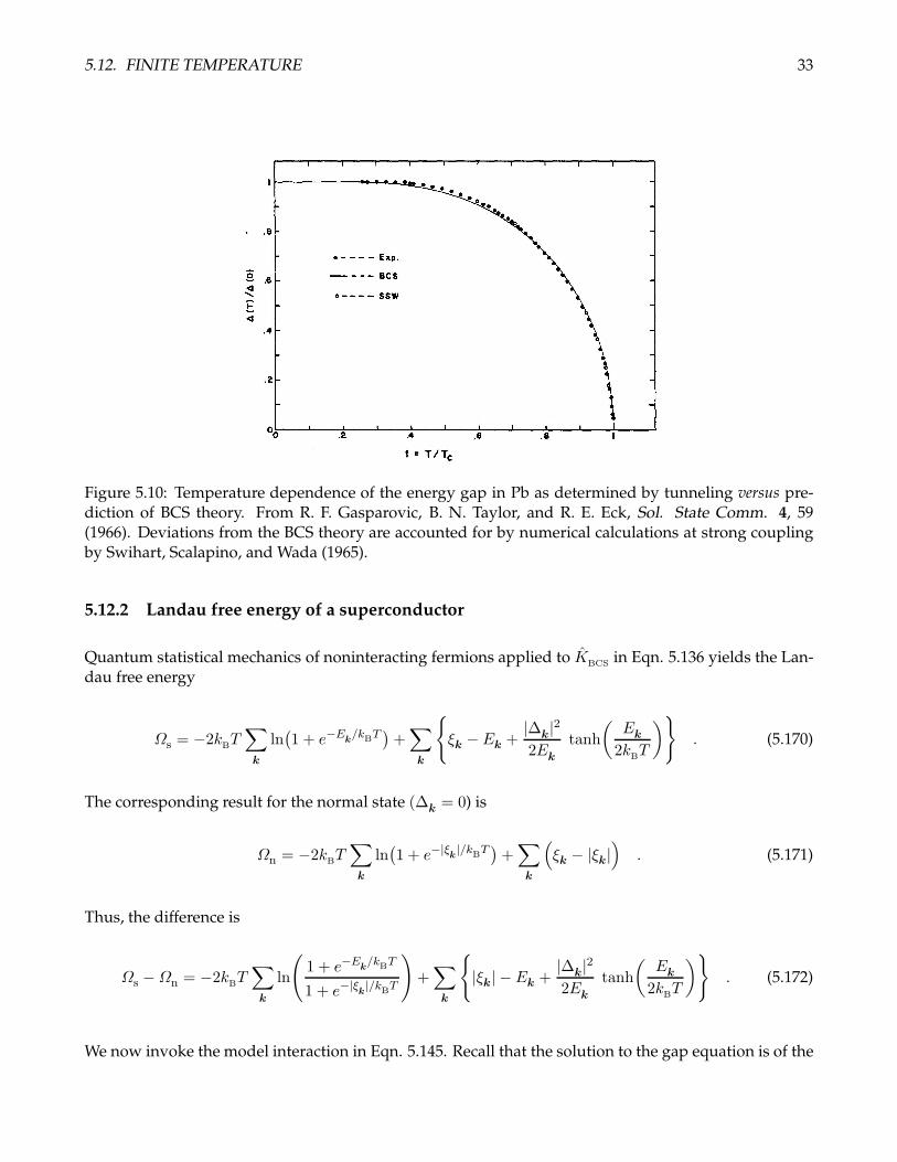
5.12. FINITE TEMPERATURE 33
Figure 5.10: Temperature dependence of the energy gap in Pb as determined by tunneling versus pre-diction of BCS theory. From R. F. Gasparovic, B. N. Taylor, and R. E. Eck, Sol. State Comm. 4, 59(1966). Deviations from the BCS theory are accounted for by numerical calculations at strong couplingby Swihart, Scalapino, and Wada (1965).
5.12.2 Landau free energy of a superconductor
Quantum statistical mechanics of noninteracting fermions applied to KBCS in Eqn. 5.136 yields the Lan-dau free energy
Ωs = −2kBT∑
k
ln(1 + e−E
k/kBT
)+∑
k
ξk − Ek +
|∆k|22Ek
tanh
(Ek
2kBT
). (5.170)
The corresponding result for the normal state (∆k = 0) is
Ωn = −2kBT∑
k
ln(1 + e−|ξ
k|/kBT
)+∑
k
(ξk − |ξk|
). (5.171)
Thus, the difference is
Ωs −Ωn = −2kBT∑
k
ln
(1 + e−E
k/kBT
1 + e−|ξk|/kBT
)+∑
k
|ξk| − Ek +
|∆k|22Ek
tanh
(Ek
2kBT
). (5.172)
We now invoke the model interaction in Eqn. 5.145. Recall that the solution to the gap equation is of the

34 CHAPTER 5. SUPERCONDUCTIVITY
form ∆k(T ) = ∆(T )Θ(~ωD − |ξk|
). We then have
Ωs −Ωn
V=
∆2
v− 1
2 g(εF)∆2
~ωD
∆
√
1 +
(~ωD
∆
)2−(~ωD
∆
)2+ sinh−1
(~ωD
∆
)
− 2 g(εF) kBT ∆
∞∫
0
ds ln(1 + e−
√1+s2 ∆/kBT
)+ 1
6 π2 g(εF) (kBT )
2 .
(5.173)
We will now expand this result in the vicinity of T = 0 and T = Tc. In the weak coupling limit,throughout this entire region we have ∆ ≪ ~ωD, so we proceed to expand in the small ratio, writing
Ωs −Ωn
V= −1
4 g(εF)∆2
1 + 2 ln
(∆0
∆
)−(
∆
2~ωD
)2
+O(∆4)
(5.174)
− 2 g(εF) kBT∆
∞∫
0
ds ln(1 + e−
√1+s2 ∆/kBT
)+ 1
6 π2 g(εF) (kBT )
2 .
where ∆0 = ∆(0) = πe−C kBTc.
T → 0+
In the limit T → 0, we find
Ωs −Ωn
V= −1
4 g(εF)∆2
1 + 2 ln
(∆0
∆
)+O
(∆2)
(5.175)
− g(εF)√
2π(kBT )3∆ e−∆/kBT + 1
6 π2 g(εF) (kBT )
2 .
Differentiating the above expression with respect to ∆, we obtain a self-consistent equation for the gap∆(T ) at low temperatures:
ln
(∆
∆0
)= −
√2πkBT
∆e−∆/kBT
(1− kBT
2∆+ . . .
)(5.176)
Thus,∆(T ) = ∆0 −
√2π∆ 0kBT e
−∆0/kBT + . . . . (5.177)
Substituting this expression into Eqn. 5.175, we find
Ωs −Ωn
V= −1
4 g(εF)∆20 − g(εF)
√2π∆0 (kBT )
3 e−∆0/kBT + 16 π
2 g(εF) (kBT )2 . (5.178)
Equating this with the condensation energy density, −H2c (T )/8π , and invoking our previous result,
∆0 = πe−C kBTc , we find
Hc(T ) = Hc(0)
1−
≈1.057︷ ︸︸ ︷13 e
2C
(T
Tc
)2+ . . .
, (5.179)
where Hc(0) =√
2π g(εF) ∆0.
5.13. PARAMAGNETIC SUSCEPTIBILITY 35
T → T−
c
In this limit, one finds
Ωs −Ωn
V= 1
2 g(εF) ln
(T
Tc
)∆2 +
7 ζ(3)
32π2g(εF)
(kBT )2∆4 +O
(∆6)
. (5.180)
This is of the standard Landau form,
Ωs −Ωn
V= a(T )∆2 + 1
2 b(T )∆4 , (5.181)
with coefficients
a(T ) = 12 g(εF)
(T
Tc− 1
), b =
7 ζ(3)
16π2g(εF)
(kBTc)2
, (5.182)
working here to lowest nontrivial order in T − Tc. The head capacity jump, according to Eqn. 1.44, is
cs(T−c )− cn(T
+c ) =
Tc[a′(Tc)
]2
b(Tc)=
4π2
7 ζ(3)g(εF) k
2BTc . (5.183)
The normal state heat capacity at T = Tc is cn = 13π
2g(εF) k2BTc , hence
cs(T−c )− cn(T
+c )
cn(T+c )
=12
7 ζ(3)= 1.43 . (5.184)
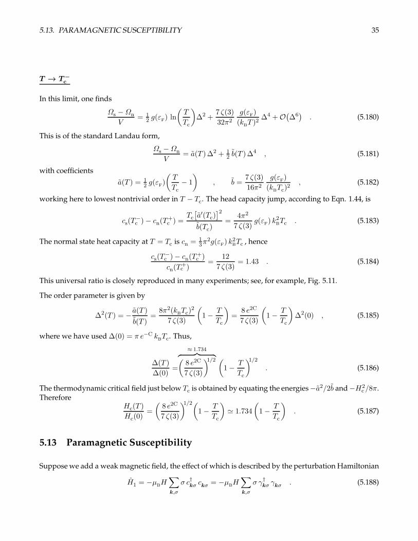
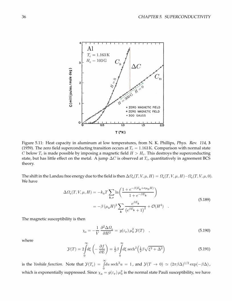
This universal ratio is closely reproduced in many experiments; see, for example, Fig. 5.11.
The order parameter is given by
∆2(T ) = − a(T )b(T )
=8π2(kBTc)
2
7 ζ(3)
(1− T
Tc
)=
8 e2C
7 ζ(3)
(1− T
Tc
)∆2(0) , (5.185)
where we have used ∆(0) = π e−C kBTc. Thus,
∆(T )
∆(0)=
≈ 1.734︷ ︸︸ ︷(8 e2C
7 ζ(3)
)1/2 (1− T
Tc
)1/2. (5.186)
The thermodynamic critical field just below Tc is obtained by equating the energies −a2/2b and −H2c /8π.
ThereforeHc(T )
Hc(0)=
(8 e2C
7 ζ(3)
)1/2(1− T
Tc
)≃ 1.734
(1− T
Tc
). (5.187)
5.13 Paramagnetic Susceptibility
Suppose we add a weak magnetic field, the effect of which is described by the perturbation Hamiltonian
H1 = −µBH∑
k,σ
σ c†kσ ckσ = −µBH∑
k,σ
σ γ†kσ γkσ . (5.188)
36 CHAPTER 5. SUPERCONDUCTIVITY
Figure 5.11: Heat capacity in aluminum at low temperatures, from N. K. Phillips, Phys. Rev. 114, 3
(1959). The zero field superconducting transition occurs at Tc = 1.163K. Comparison with normal stateC below Tc is made possible by imposing a magnetic field H > Hc. This destroys the superconductingstate, but has little effect on the metal. A jump ∆C is observed at Tc, quantitatively in agreement BCStheory.
The shift in the Landau free energy due to the field is then ∆Ωs(T, V, µ,H) = Ωs(T, V, µ,H)−Ωs(T, V, µ, 0).We have
∆Ωs(T, V, µ,H) = −kBT∑
k,σ
ln
(1 + e−β(E
k+σµBH)
1 + e−βEk
)
= −β (µBH)2∑
k
eβEk
(eβEk + 1
)2 +O(H4) .
(5.189)
The magnetic susceptibility is then
χs = − 1
V
∂2∆Ωs
∂H2= g(εF)µ
2B Y(T ) , (5.190)
where
Y(T ) = 2
∞∫
0
dξ
(− ∂f
∂E
)= 1
2β
∞∫
0
dξ sech2(12β√ξ2 +∆2
)(5.191)
is the Yoshida function. Note that Y(Tc) =∞∫0
du sech2u = 1 , and Y(T → 0) ≃ (2πβ∆)1/2 exp(−β∆) ,
which is exponentially suppressed. Since χn = g(εF)µ2B is the normal state Pauli susceptibility, we have
5.13. PARAMAGNETIC SUSCEPTIBILITY 37
that the ratio of superconducting to normal state susceptibilities is χs(T )/χn(T ) = Y(T ). This vanishesexponentially as T → 0 because it takes a finite energy ∆ to create a Bogoliubov quasiparticle out of thespin singlet BCS ground state.
In metals, the nuclear spins experience a shift in their resonance energy in the presence of an externalmagnetic field, due to their coupling to conduction electrons via the hyperfine interaction. This is calledthe Knight shift, after Walter Knight, who first discovered this phenomenon at Berkeley in 1949. Themagnetic field polarizes the metallic conduction electrons, which in turn impose an extra effective field,through the hyperfine coupling, on the nuclei. In superconductors, the electrons remain unpolarized ina weak magnetic field owing to the superconducting gap. Thus there is no Knight shift.
As we have seen from the Ginzburg-Landau theory, when the field is sufficiently strong, supercon-ductivity is destroyed (type I), or there is a mixed phase at intermediate fields where magnetic fluxpenetrates the superconductor in the form of vortex lines. Our analysis here is valid only for weakfields.