CONTENTS

S.NO TOPIC PAGE NO.

UNIT I ELECTROSTATICS – I 1

1.1 Introduction to electrostatics 1

1.2 Sources and effects of electromagnetic fields 2

1.3 Divergence, Curl 7

1.4 Vector fields(dot, cross product) 7

1.5 Coordinate Systems 8

1.6 transformation of coordinates 15

1.7 theorems and applications 25

1.8 Electric field intensity & Coulomb’s Law 31

1.9 Field due to discrete and continuous charges 33

1.10 Gauss’s law and applications. 35 UNIT II ELECTROSTATICS – II 36

2.1 Electric potential 39

2.2 Electric field and equipotential plots 39

2.3 Uniform and Non-Uniform field 40

2.4 Utilization factor 42

2.5 Electric field in free space, conductors, dielectrics 44

2.6 Dielectric polarization 45

2.7 Dielectric strength 46

2.8 Electric field in multiple dielectrics 47

2.9 Boundary conditions 48

2.10 Poisson’s and Laplace’sequations 63

2.11 Capacitance, Energy density, Applications 59 UNIT III MAGNETOSTATICS 67

3.1 Lorentz force, magnetic field intensity (H) 67

3.2 Biot–Savart’s Law 67

3.3 Ampere’s Circuit Law 70

3.4 H due to straight conductors 71

3.5 circular loop, infinite sheet of current, 72

3.6 Magnetic flux density (B) – B in free space 72

3.7 conductor, magnetic materials 73

3.8 Magnetization, 73

3.9 Magnetic field in multiple media 74

3.10 Boundary conditions 78

3.11 scalar and vector potential, Poisson’s Equation 74

3.12 Magnetic force, Torque 73 UNIT IV ELECTRODYNAMIC FIELDS 82

4.1 Magnetic Circuits 82

4.2 Faraday’s law 83

4.3 Transformer and motional EMF 85

4.4 Displacement current 86

4.5 Maxwell’s equations (differential and integral form) 87

4.6 Relation between field theory and circuit theory 89

4.7 Relation between field theory and circuit theory Applications. 92 UNIT V ELECTROMAGNETIC WAVES 99

5.1 Electromagnetic wave generation and equations 99

5.2 Wave parameters; 100

5.3 velocity, intrinsic impedance 107

5.4 propagation constant – Waves in free space 107

5.5 lossy and lossless dielectrics 107

5.6 conductors- skin depth 109

5.7 Poynting vector – Plane wave reflection and refractions 112

5.8 Standing Wave – Applications 125

Question Bank 141

1

UNIT – 1 INTRODUCTION

Electromagnetic theory is a discipline concerned with the study of charges at rest and in

motion. Electromagnetic principles are fundamental to the study of electrical engineering and

physics. Electromagnetic theory is also indispensable to the understanding, analysis and design of

various electrical, electromechanical and electronic systems. Some of the branches of study where

Electromagnetic principles find applications are:

1. RF communication

2. Microwave Engineering

3. Antennas

4. Electrical Machines

5. Satellite Communication

6. Atomic and nuclear research

7. Radar Technology

8. Remote sensing

9. EMI EMC

10. Quantum Electronics

11. VLSI

Electromagnetic theory is a prerequisite for a wide spectrum of studies in the field of Electrical

Sciences and Physics. Electromagnetic theory can be thought of as generalization of circuit theory.

There are certain situations that can be handled exclusively in terms of field theory. In

electromagnetic theory, the quantities involved can be categorized as source quantities and field

quantities. Source of electromagnetic field is electric charges: either at rest or in motion. However

an electromagnetic field may cause a redistribution of charges that in turn change the field and

hence the separation of cause and effect is not always visible.

Sources of EMF:

Current carrying conductors.

Mobile phones.

Microwave oven.

Computer and Television screen.

High voltage Power lines.

Effects of Electromagnetic fields:

Plants and Animals.

Humans.

Electrical components.

Fields are classified as

2

Scalar field

Vector field.

Electric charge is a fundamental property of matter. Charge exist only in positive or negative

integral multiple of electronic charge, -e, e= 1.60 × 10-19 coulombs. [It may be noted here that in

1962, Murray Gell-Mann hypothesized Quarks as the basic building blocks of matters. Quarks were

predicted to carry a fraction of electronic charge and the existence of Quarks have been

experimentally verified.] Principle of conservation of charge states that the total charge (algebraic

sum of positive and negative charges) of an isolated system remains unchanged, though the

charges may redistribute under the influence of electric field. Kirchhoff's Current Law (KCL) is an

assertion of the conservative property of charges under the implicit assumption that there is no

accumulation of charge at the junction.

Electromagnetic theory deals directly with the electric and magnetic field vectors where as

circuit theory deals with the voltages and currents. Voltages and currents are integrated effects of

electric and magnetic fields respectively. Electromagnetic field problems involve three space

variables along with the time variable and hence the solution tends to become correspondingly

complex. Vector analysis is a mathematical tool with which electromagnetic concepts are more

conveniently expressed and best comprehended. Since use of vector analysis in the study of

electromagnetic field theory results in real economy of time and thought, we first introduce the

concept of vector analysis.

Vector Analysis:

The quantities that we deal in electromagnetic theory may be either scalar or vectors [There

are other class of physical quantities called Tensors: where magnitude and direction vary with co

ordinate axes]. Scalars are quantities characterized by magnitude only and algebraic sign. A quantity

that has direction as well as magnitude is called a vector. Both scalar and vector quantities are

function of time and position . A field is a function that specifies a particular quantity everywhere in

a region. Depending upon the nature of the quantity under consideration, the field may be a vector

or a scalar field. Example of scalar field is the electric potential in a region while electric or magnetic

fields at any point is the example of vector field.

A vector can be written as, ,

where, is the magnitude

and is the unit vector which has unit magnitude and same direction as that of .

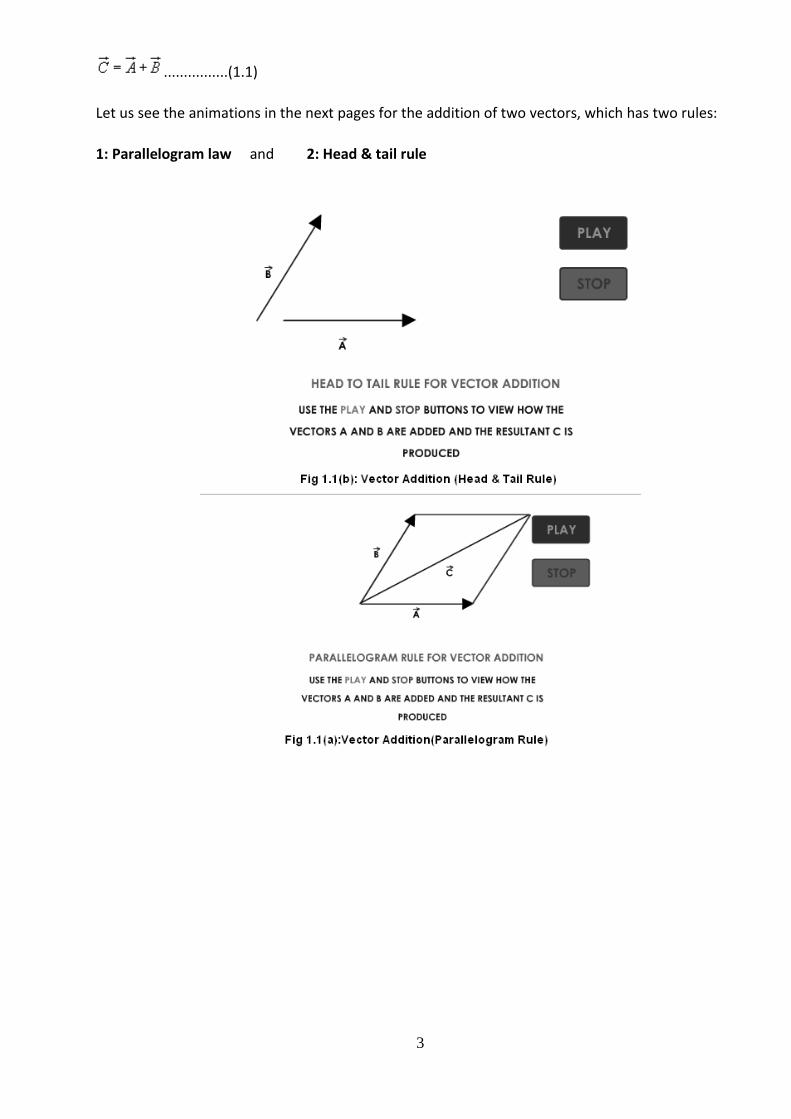
Two vector and are added together to give another vector . We have

3

................(1.1)

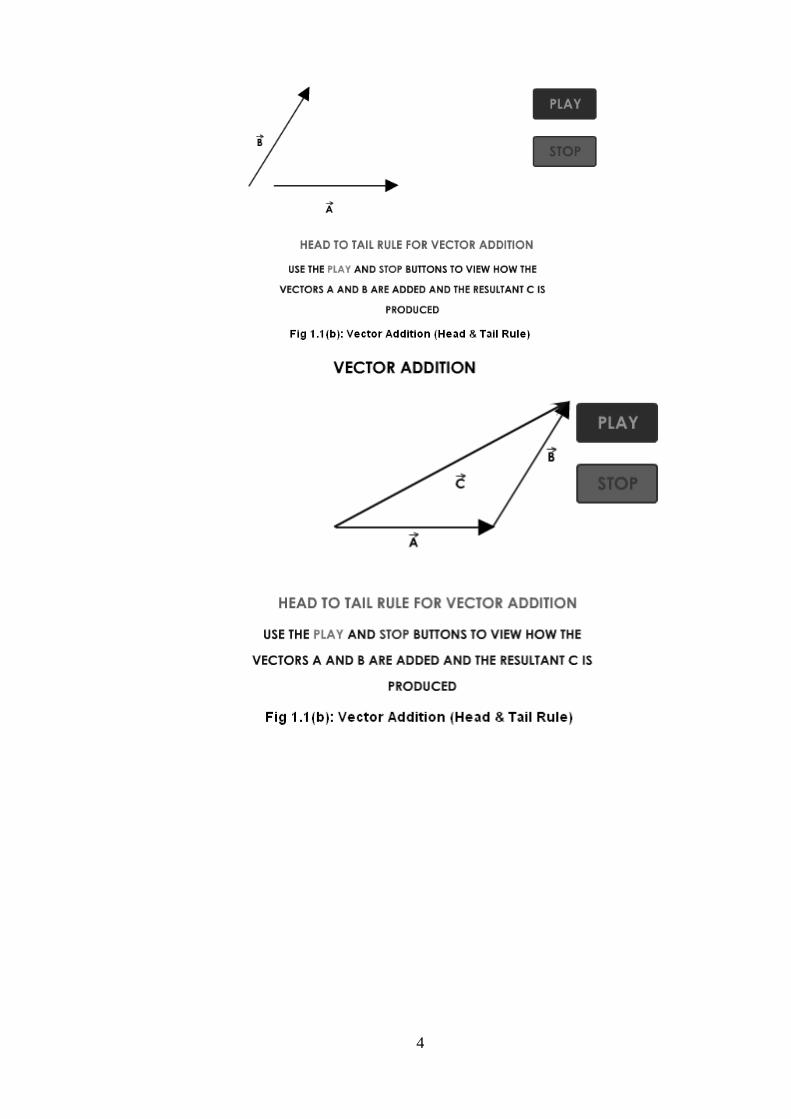
Let us see the animations in the next pages for the addition of two vectors, which has two rules:

1: Parallelogram law and 2: Head & tail rule

4

5

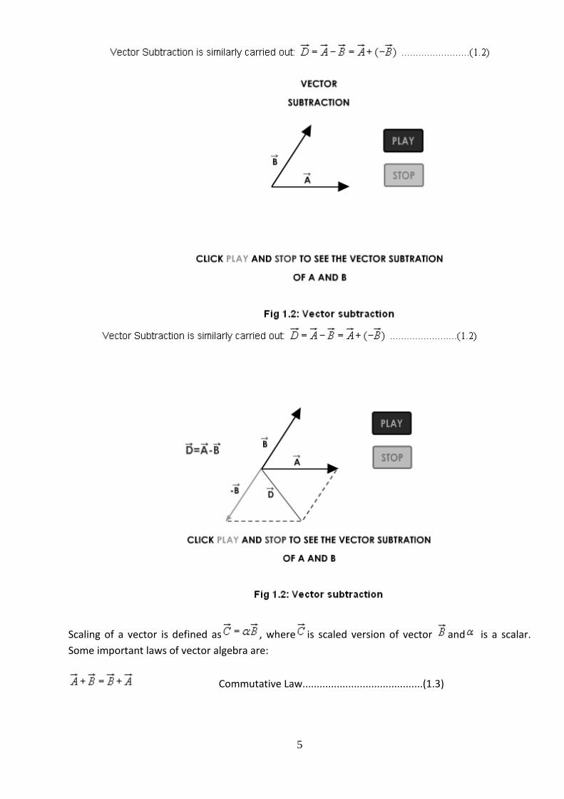
Scaling of a vector is defined as , where is scaled version of vector and is a scalar.

Some important laws of vector algebra are:

Commutative Law..........................................(1.3)

6

Associative Law.............................................(1.4)

Distributive Law ............................................(1.5)

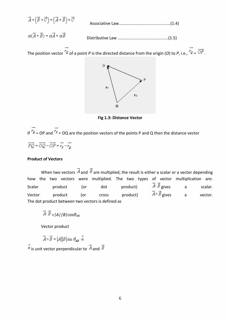
The position vector of a point P is the directed distance from the origin (O) to P, i.e., = .

Fig 1.3: Distance Vector

If = OP and = OQ are the position vectors of the points P and Q then the distance vector

Product of Vectors

When two vectors and are multiplied, the result is either a scalar or a vector depending

how the two vectors were multiplied. The two types of vector multiplication are:

Scalar product (or dot product) gives a scalar.

Vector product (or cross product) gives a vector.

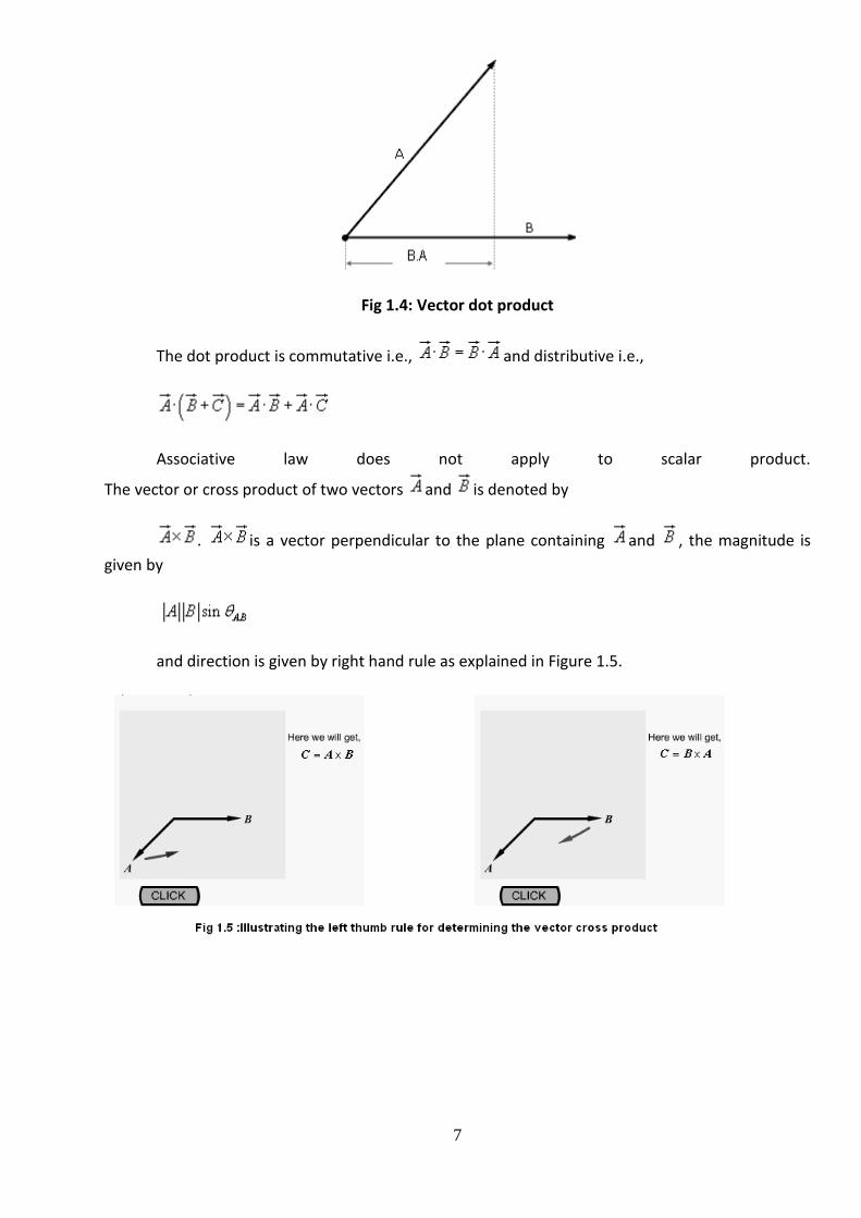
The dot product between two vectors is defined as

=|A||B|cosθAB

Vector product

is unit vector perpendicular to and

7

Fig 1.4: Vector dot product

The dot product is commutative i.e., and distributive i.e.,

Associative law does not apply to scalar product.

The vector or cross product of two vectors and is denoted by

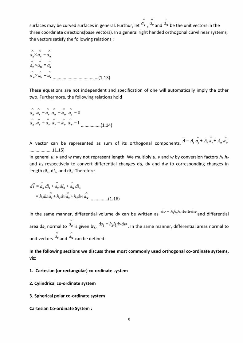
. is a vector perpendicular to the plane containing and , the magnitude is

given by

and direction is given by right hand rule as explained in Figure 1.5.

8

............................................................................................(1.7)

where is the unit vector given by, .

The following relations hold for vector product.

= i.e., cross product is non commutative ..........(1.8)

i.e., cross product is distributive.......................(1.9)

i.e., cross product is non associative..............(1.10)

Scalar and vector triple product :

Scalar triple product .................................(1.11)

Vector triple product ...................................(1.12)

Co-ordinate Systems

In order to describe the spatial variations of the quantities, we require using appropriate co-

ordinate system. A point or vector can be represented in a curvilinear coordinate system that may

be orthogonal or non-orthogonal .

An orthogonal system is one in which the co-ordinates are mutually perpendicular. Non-orthogonal

co-ordinate systems are also possible, but their usage is very limited in practice .

Let u = constant, v = constant and w = constant represent surfaces in a coordinate system, the

9

surfaces may be curved surfaces in general. Furthur, let , and be the unit vectors in the

three coordinate directions(base vectors). In a general right handed orthogonal curvilinear systems,

the vectors satisfy the following relations :

.....................................(1.13)

These equations are not independent and specification of one will automatically imply the other

two. Furthermore, the following relations hold

................(1.14)

A vector can be represented as sum of its orthogonal components,

...................(1.15)

In general u, v and w may not represent length. We multiply u, v and w by conversion factors h1,h2

and h3 respectively to convert differential changes du, dv and dw to corresponding changes in

length dl1, dl2, and dl3. Therefore

...............(1.16)

In the same manner, differential volume dv can be written as and differential

area ds1 normal to is given by, . In the same manner, differential areas normal to

unit vectors and can be defined.

In the following sections we discuss three most commonly used orthogonal co-ordinate systems,

viz:

1. Cartesian (or rectangular) co-ordinate system

2. Cylindrical co-ordinate system

3. Spherical polar co-ordinate system

Cartesian Co-ordinate System :

10

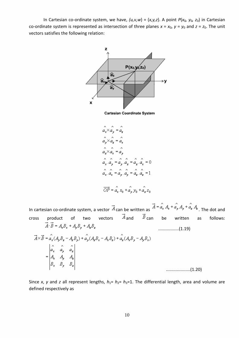
In Cartesian co-ordinate system, we have, (u,v,w) = (x,y,z). A point P(x0, y0, z0) in Cartesian

co-ordinate system is represented as intersection of three planes x = x0, y = y0 and z = z0. The unit

vectors satisfies the following relation:

In cartesian co-ordinate system, a vector can be written as . The dot and

cross product of two vectors and can be written as follows:

.................(1.19)

....................(1.20)

Since x, y and z all represent lengths, h1= h2= h3=1. The differential length, area and volume are

defined respectively as

11

................(1.21)

.................................(1.22)

Cylindrical Co-ordinate System :

For cylindrical coordinate systems we have a point is determined as

the point of intersection of a cylindrical surface r = r0, half plane containing the z-axis and making an

angle ; with the xz plane and a plane parallel to xy plane located at z=z0 as shown in figure 7

on next page.

In cylindrical coordinate system, the unit vectors satisfy the following relations

A vector can be written as , ...........................(1.24)

The differential length is defined as,

......................(1.25)

.....................(1.23)

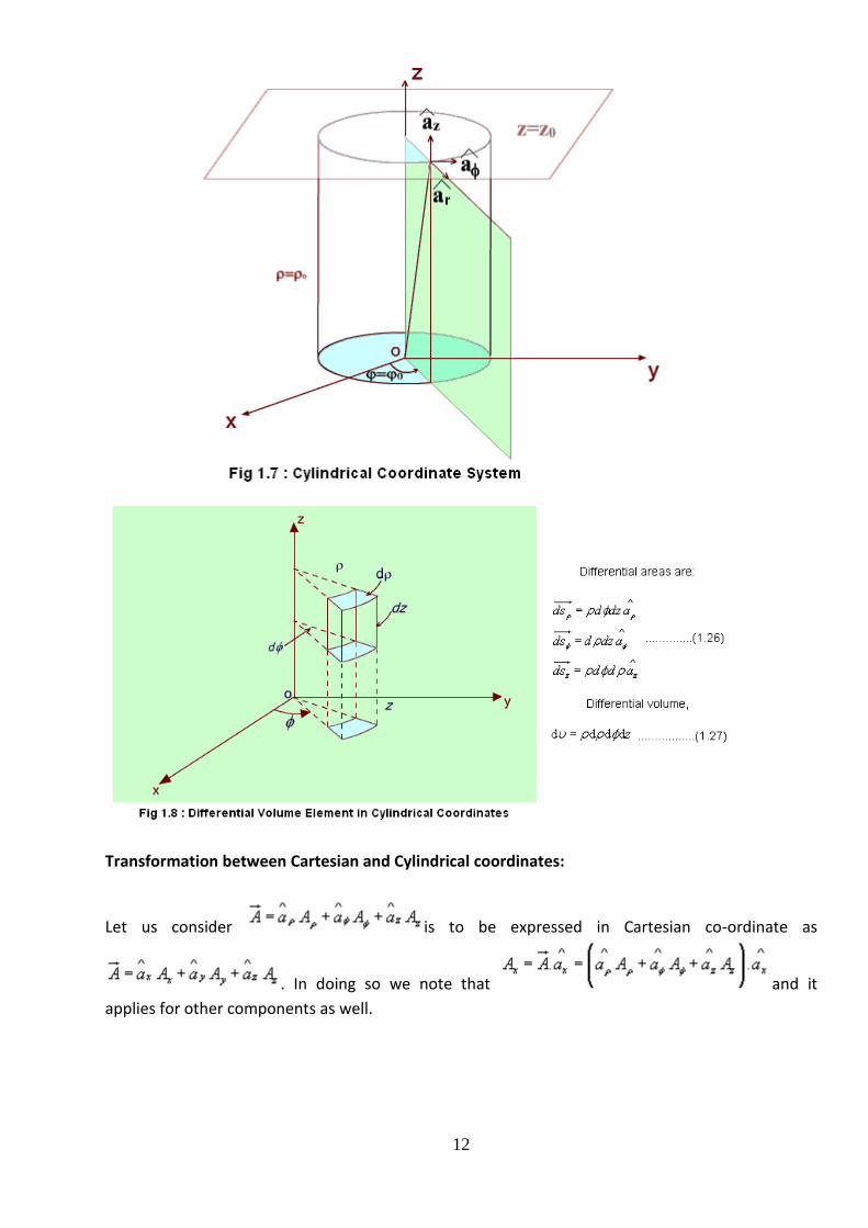
12

Transformation between Cartesian and Cylindrical coordinates:

Let us consider is to be expressed in Cartesian co-ordinate as

. In doing so we note that and it

applies for other components as well.

13

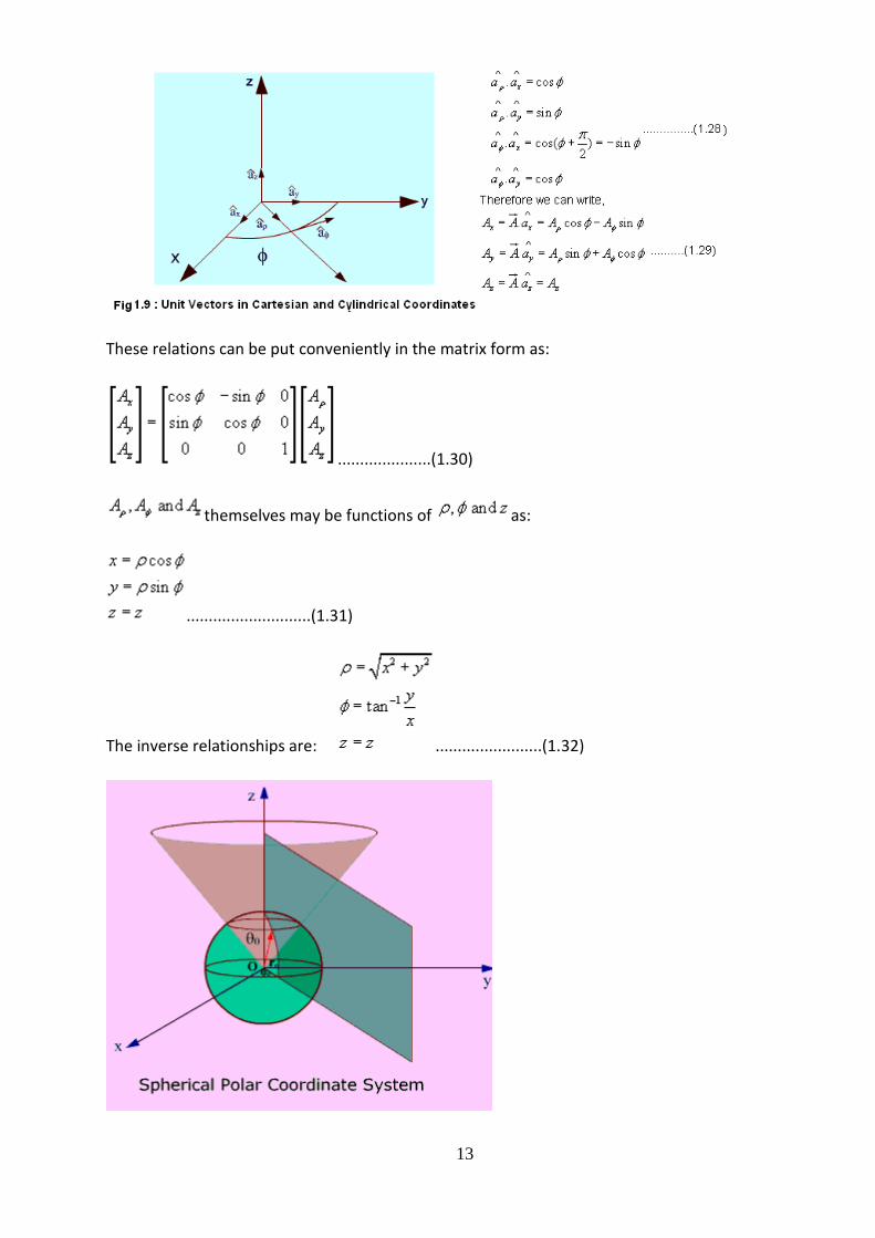
These relations can be put conveniently in the matrix form as:

.....................(1.30)

themselves may be functions of as:

............................(1.31)

The inverse relationships are: ........................(1.32)

14

Fig 1.10: Spherical Polar Coordinate System

Thus we see that a vector in one coordinate system is transformed to another coordinate system

through two-step process: Finding the component vectors and then variable transformation.

Spherical Polar Coordinates:

For spherical polar coordinate system, we have, . A point is

represented as the intersection of

(i) Spherical surface r=r0

(ii) Conical surface ,and

(iii) half plane containing z-axis making angle with the xz plane as shown in the figure 1.10.

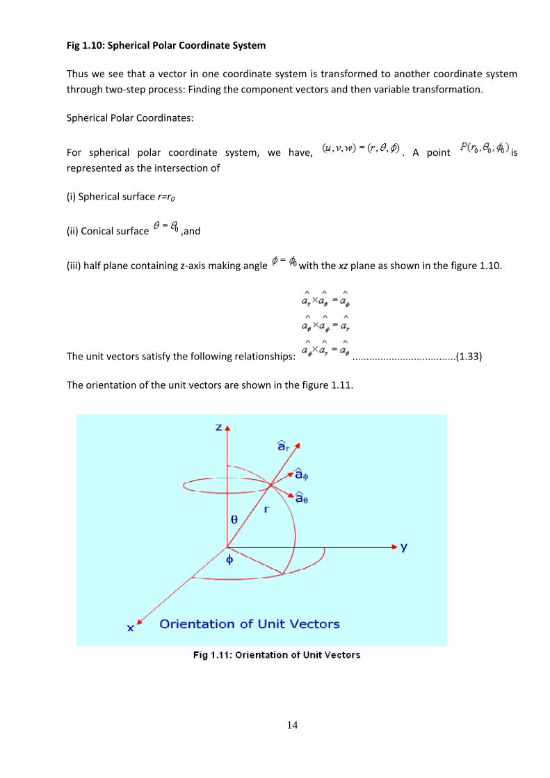
The unit vectors satisfy the following relationships: .....................................(1.33)

The orientation of the unit vectors are shown in the figure 1.11.

15

A vector in spherical polar co-ordinates is written as : and

For spherical polar coordinate system we have h1=1, h2= r and h3= .

Fig 1.12(b) : Exploded view

With reference to the Figure 1.12, the elemental areas are:

.......................(1.34)

and elementary volume is given by

........................(1.35)

Coordinate transformation between rectangular and spherical polar:

16

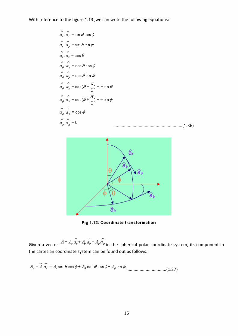
With reference to the figure 1.13 ,we can write the following equations:

........................................................(1.36)

Given a vector in the spherical polar coordinate system, its component in

the cartesian coordinate system can be found out as follows:

.................................(1.37)

17

Similarly,

.................................(1.38a)

.................................(1.38b)

The above equation can be put in a compact form:

.................................(1.39)

The components themselves will be functions of . are related to

x,y and z as:

....................(1.40)

and conversely,

.......................................(1.41a)

.................................(1.41b)

.....................................................(1.41c)

Using the variable transformation listed above, the vector components, which are functions of

variables of one coordinate system, can be transformed to functions of variables of other

coordinate system and a total transformation can be done.

Line, surface and volume integrals

In electromagnetic theory, we come across integrals, which contain vector functions. Some

representative integrals are listed below:

18

In the above integrals, and respectively represent vector and scalar function of space

coordinates. C,S and V represent path, surface and volume of integration. All these integrals are

evaluated using extension of the usual one-dimensional integral as the limit of a sum, i.e., if a

function f(x) is defined over arrange a to b of values of x, then the integral is given by

.................................(1.42)

where the interval (a,b) is subdivided into n continuous interval of lengths .

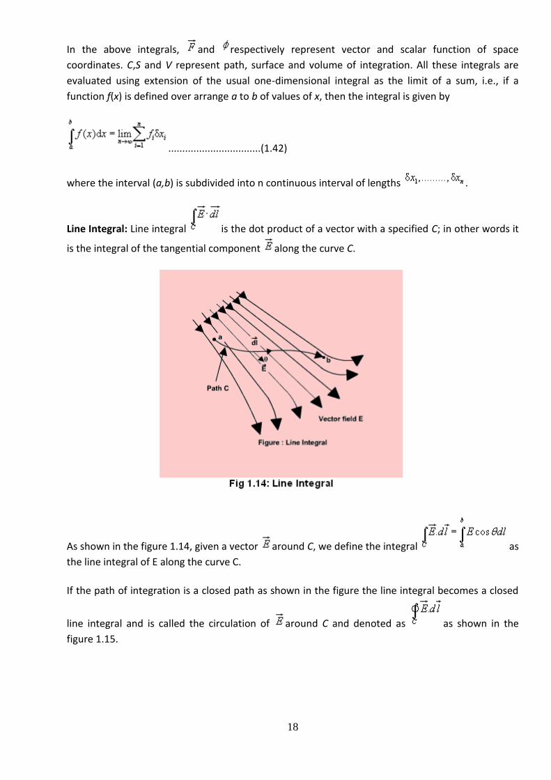
Line Integral: Line integral is the dot product of a vector with a specified C; in other words it

is the integral of the tangential component along the curve C.

As shown in the figure 1.14, given a vector around C, we define the integral as

the line integral of E along the curve C.

If the path of integration is a closed path as shown in the figure the line integral becomes a closed

line integral and is called the circulation of around C and denoted as as shown in the

figure 1.15.

19

Fig 1.15: Closed Line Integral

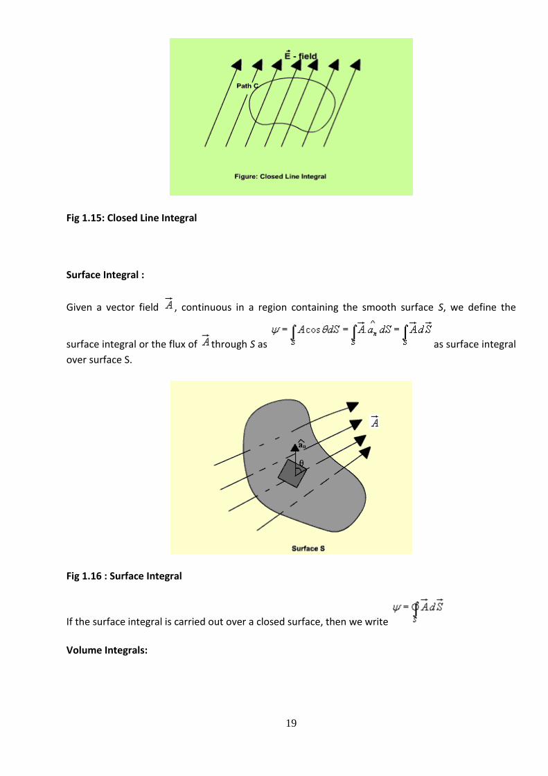
Surface Integral :

Given a vector field , continuous in a region containing the smooth surface S, we define the

surface integral or the flux of through S as as surface integral

over surface S.

Fig 1.16 : Surface Integral

If the surface integral is carried out over a closed surface, then we write

Volume Integrals:

20

We define or as the volume integral of the scalar function f(function of spatial

coordinates) over the volume V. Evaluation of integral of the form can be carried out as a

sum of three scalar volume integrals, where each scalar volume integral is a component of the

vector

The Del Operator :

The vector differential operator was introduced by Sir W. R. Hamilton and later on developed by

P. G. Tait.

Mathematically the vector differential operator can be written in the general form as:

.................................(1.43)

In Cartesian coordinates:

................................................(1.44)

In cylindrical coordinates:

...........................................(1.45)

and in spherical polar coordinates:

.................................(1.46)

Gradient of a Scalar function:

Let us consider a scalar field V(u,v,w) , a function of space coordinates.

Gradient of the scalar field V is a vector that represents both the magnitude and direction of the

maximum space rate of increase of this scalar field V.

21

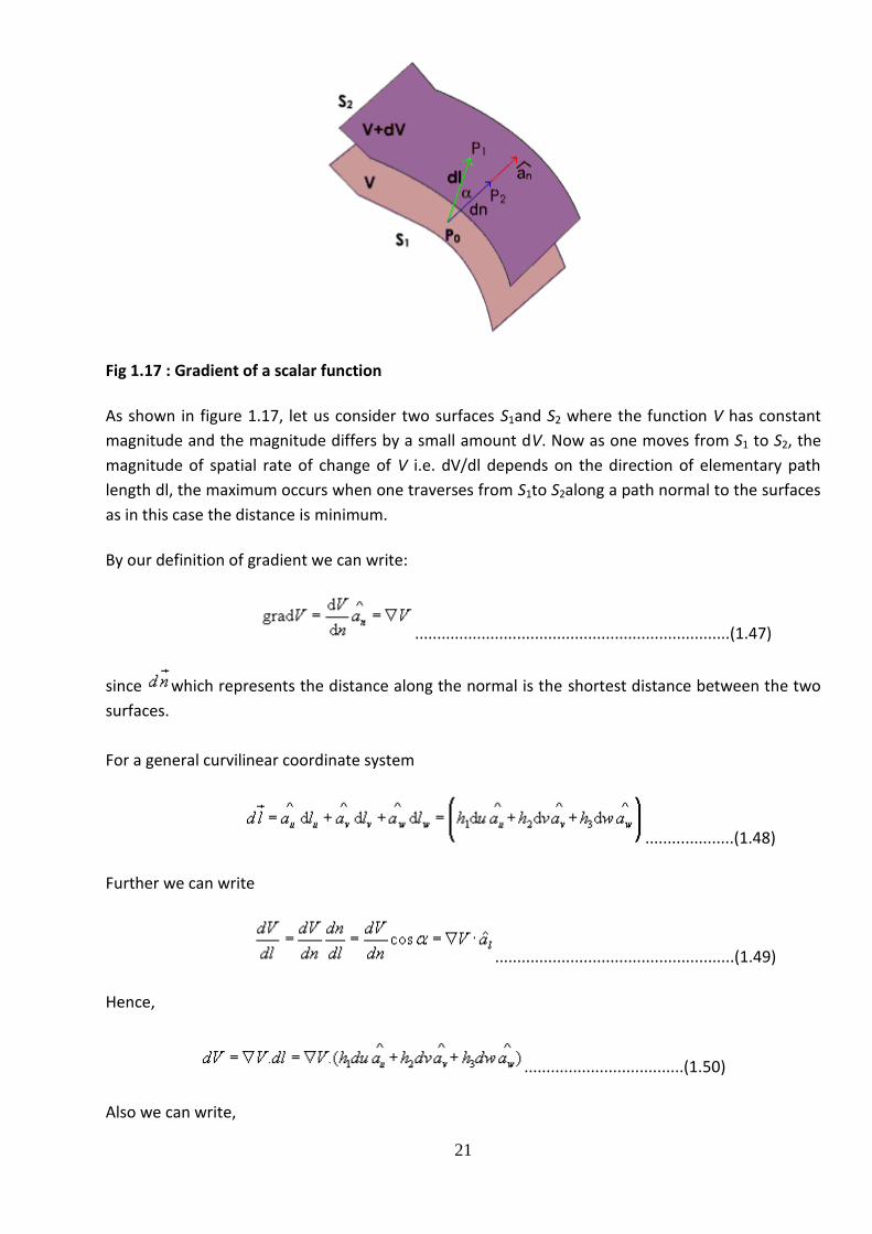
Fig 1.17 : Gradient of a scalar function

As shown in figure 1.17, let us consider two surfaces S1and S2 where the function V has constant

magnitude and the magnitude differs by a small amount dV. Now as one moves from S1 to S2, the

magnitude of spatial rate of change of V i.e. dV/dl depends on the direction of elementary path

length dl, the maximum occurs when one traverses from S1to S2along a path normal to the surfaces

as in this case the distance is minimum.

By our definition of gradient we can write:

.......................................................................(1.47)

since which represents the distance along the normal is the shortest distance between the two

surfaces.

For a general curvilinear coordinate system

....................(1.48)

Further we can write

......................................................(1.49)

Hence,

....................................(1.50)

Also we can write,

22

............................(1.51)

By comparison we can write,

.............................................(1.52)

Hence for the Cartesian, cylindrical and spherical polar coordinate system, the expressions for

gradient can be written as:

In Cartesian coordinates:

...........................................(1.53)

In cylindrical coordinates:

...........................................(1.54)

and in spherical polar coordinates:

.........................................(1.55)

The following relationships hold for gradient operator.

................................................(1.56)

where U and V are scalar functions and n is an integer.

23

It may further be noted that since magnitude of depends on the direction of dl, it is

called the directional derivative. If is called the scalar potential function of the vector

function .

Divergence of a Vector Field:

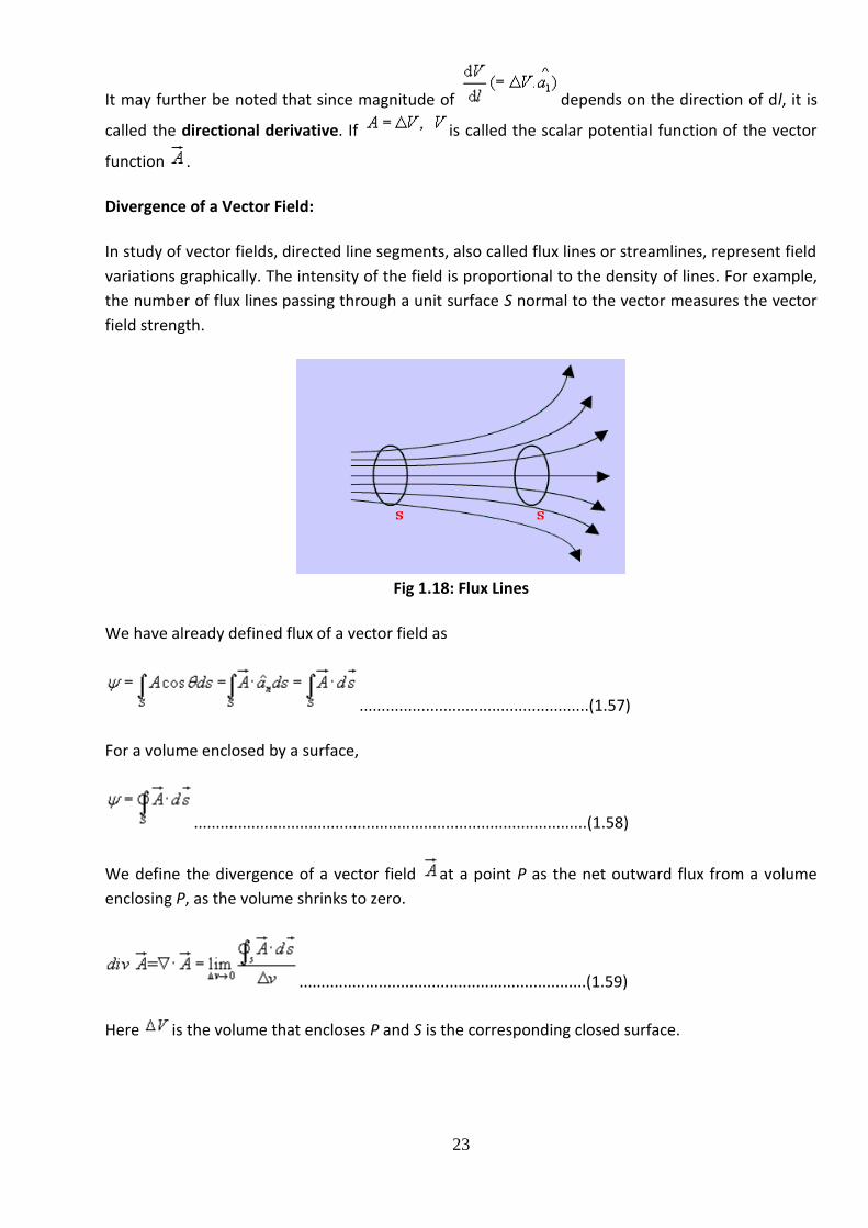
In study of vector fields, directed line segments, also called flux lines or streamlines, represent field

variations graphically. The intensity of the field is proportional to the density of lines. For example,

the number of flux lines passing through a unit surface S normal to the vector measures the vector

field strength.

Fig 1.18: Flux Lines

We have already defined flux of a vector field as

....................................................(1.57)

For a volume enclosed by a surface,

.........................................................................................(1.58)

We define the divergence of a vector field at a point P as the net outward flux from a volume

enclosing P, as the volume shrinks to zero.

.................................................................(1.59)

Here is the volume that encloses P and S is the corresponding closed surface.

24

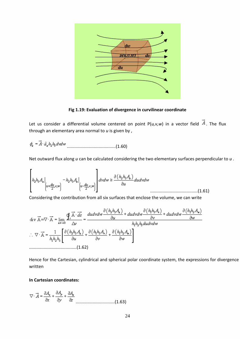
Fig 1.19: Evaluation of divergence in curvilinear coordinate

Let us consider a differential volume centered on point P(u,v,w) in a vector field . The flux

through an elementary area normal to u is given by ,

........................................(1.60)

Net outward flux along u can be calculated considering the two elementary surfaces perpendicular to u .

.......................................(1.61)

Considering the contribution from all six surfaces that enclose the volume, we can write

.......................................(1.62)

Hence for the Cartesian, cylindrical and spherical polar coordinate system, the expressions for divergence can be

written as:

In Cartesian coordinates:

................................(1.63)

25

In cylindrical coordinates:

....................................................................(1.64)

and in spherical polar coordinates:

......................................(1.65)

In connection with the divergence of a vector field, the following can be noted

Divergence of a vector field gives a scalar.

..............................................................................(1.66)

Divergence theorem :

Divergence theorem states that the volume integral of the divergence of vector field is equal to the

net outward flux of the vector through the closed surface that bounds the volume. Mathematically,

Proof:

Let us consider a volume V enclosed by a surface S . Let us subdivide the volume in large number of

cells. Let the kth cell has a volume and the corresponding surface is denoted by Sk. Interior to

the volume, cells have common surfaces. Outward flux through these common surfaces from one

cell becomes the inward flux for the neighboring cells. Therefore when the total flux from these

cells are considered, we actually get the net outward flux through the surface surrounding the

volume. Hence we can write:

......................................(1.67)

In the limit, that is when and the right hand of the expression can be written as

.

Hence we get , which is the divergence theorem.

26

Curl of a vector field:

We have defined the circulation of a vector field A around a closed path as .

Curl of a vector field is a measure of the vector field's tendency to rotate about a point. Curl , also

written as is defined as a vector whose magnitude is maximum of the net circulation per unit

area when the area tends to zero and its direction is the normal direction to the area when the area

is oriented in such a way so as to make the circulation maximum.

Therefore, we can write:

......................................(1.68)

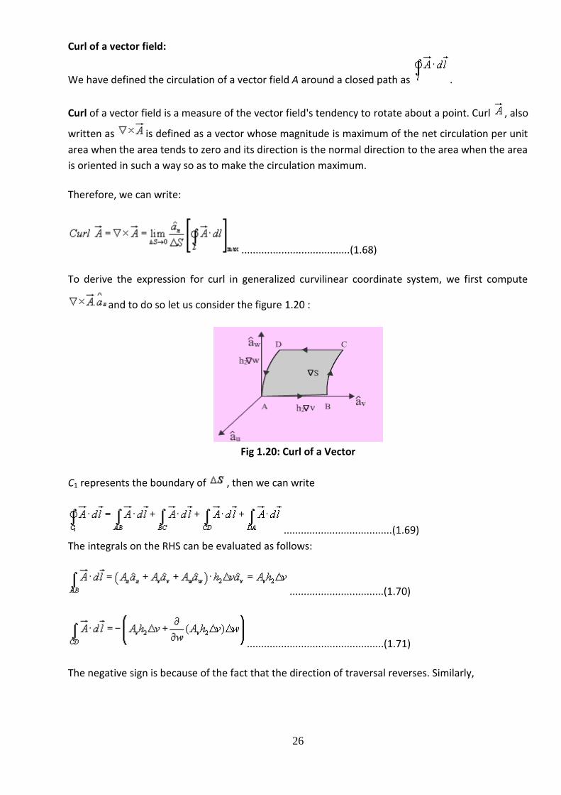
To derive the expression for curl in generalized curvilinear coordinate system, we first compute

and to do so let us consider the figure 1.20 :

Fig 1.20: Curl of a Vector

C1 represents the boundary of , then we can write

......................................(1.69)

The integrals on the RHS can be evaluated as follows:

.................................(1.70)

................................................(1.71)

The negative sign is because of the fact that the direction of traversal reverses. Similarly,

27

..................................................(1.72)

............................................................................(1.73)

Adding the contribution from all components, we can write:

........................................................................(1.74)

Therefore, ........................(1.75)

In the same manner if we compute for and we can write,

.......(1.76)

This can be written as,

......................................................(1.77)

In Cartesian coordinates: .......................................(1.78)

In Cylindrical coordinates, ....................................(1.79)

28

In Spherical polar coordinates, ..............(1.80)

Curl operation exhibits the following properties:

..............(1.81)

Stoke's theorem :

It states that the circulation of a vector field around a closed path is equal to the integral of

over the surface bounded by this path. It may be noted that this equality holds provided

and are continuous on the surface.

i.e,

..............(1.82)

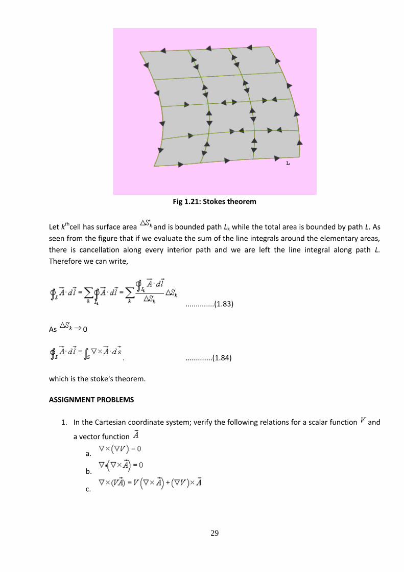
Proof: Let us consider an area S that is subdivided into large number of cells as shown in the figure

1.21.

29

Fig 1.21: Stokes theorem

Let kthcell has surface area and is bounded path Lk while the total area is bounded by path L. As

seen from the figure that if we evaluate the sum of the line integrals around the elementary areas,

there is cancellation along every interior path and we are left the line integral along path L.

Therefore we can write,

..............(1.83)

As 0

. .............(1.84)

which is the stoke's theorem.

ASSIGNMENT PROBLEMS

1. In the Cartesian coordinate system; verify the following relations for a scalar function and

a vector function

a.

b.

c.

30

2. An electric field expressed in spherical polar coordinates is given by . Determine

and at a point .

3. Evaluate over the surface of a sphere of radius centered at the origin.

4. Find the divergence of the radial vector field given by .

5. A vector function is defined by . Find around the contour shown in

the figure P1.3 . Evaluate over the shaded area and verify that

Figure P1.3

31

Unit II Electrostatics

In this chapter we will discuss on the followings:

1. Coulomb's Law 2. Electric Field & Electric Flux Density 3. Gauss's Law with Application 4. Electrostatic Potential, Equipotential Surfaces 5. Boundary Conditions for Static Electric Fields 6. Capacitance and Capacitors 7. Electrostatic Energy 8. Laplace's and Poisson's Equations 9. Uniqueness of Electrostatic Solutions 10. Method of Images 11. Solution of Boundary Value Problems in Different

Coordinate Systems

Introduction

In the previous chapter we have covered the essential mathematical tools needed to study EM fields. We have already mentioned in the previous chapter that electric charge is a fundamental property of matter and charge exist in integral multiple of electronic charge. Electrostatics can be defined as the study of electric charges at rest. Electric fields have their sources in electric charges.

( Note: Almost all real electric fields vary to some extent with time. However, for many problems, the field variation is slow and the field may be considered as static. For some other cases spatial distribution is nearly same as for the static case even though the actual field may vary with time. Such cases are termed as quasi-static.)

In this chapter we first study two fundamental laws governing the electrostatic fields, viz, (1) Coulomb's Law and (2) Gauss's Law. Both these law have experimental basis. Coulomb's law is applicable in finding electric field due to any charge distribution, Gauss's law is easier to use when the distribution is symmetrical.

Coulomb's Law

32

Coulomb's Law states that the force between two point charges Q1and Q2 is directly proportional to the product of the charges and inversely proportional to the square of the distance between them.

Point charge is a hypothetical charge located at a single point in space. It is an idealised model of a particle having an electric charge.

Mathematically, ,where k is the proportionality constant.

In SI units, Q1 and Q2 are expressed in Coulombs(C) and R is in meters.

Force F is in Newtons (N) and , is called the permittivity of free space.

(We are assuming the charges are in free space. If the charges are any other

dielectric medium, we will use instead where is called the relative permittivity or the dielectric constant of the medium).

Therefore .......................(2.1)

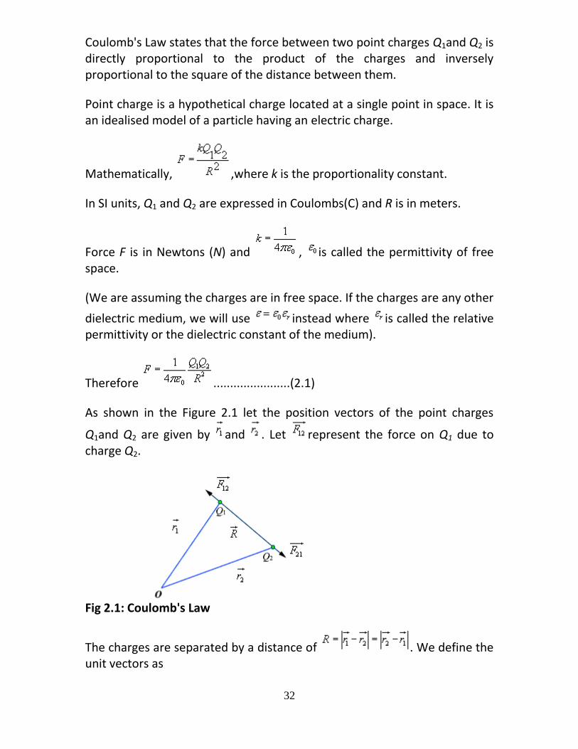
As shown in the Figure 2.1 let the position vectors of the point charges

Q1and Q2 are given by and . Let represent the force on Q1 due to charge Q2.

Fig 2.1: Coulomb's Law

The charges are separated by a distance of . We define the unit vectors as

33

and ..................................(2.2)

can be defined as . Similarly the force on

Q1 due to charge Q2 can be calculated and if represents this force then

we can write

When we have a number of point charges, to determine the force on a particular charge due to all other charges, we apply principle of superposition. If we have N number of charges Q1,Q2,.........QN located

respectively at the points represented by the position vectors , ,...... ,

the force experienced by a charge Q located at is given by,

.................................(2.3)

Electric Field

The electric field intensity or the electric field strength at a point is defined as the force per unit charge. That is

or, .......................................(2.4)

The electric field intensity E at a point r (observation point) due a point

charge Q located at (source point) is given by:

..........................................(2.5)

For a collection of N point charges Q1 ,Q2 ,.........QN located at , ,...... ,

the electric field intensity at point is obtained as

........................................(2.6)

34

The expression (2.6) can be modified suitably to compute the electric filed due to a continuous distribution of charges.

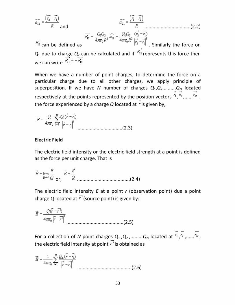
In figure 2.2 we consider a continuous volume distribution of charge (t) in the region denoted as the source region.

For an elementary charge , i.e. considering this charge as point charge, we can write the field expression as:

.............(2.7)

Fig 2.2: Continuous Volume Distribution of Charge

When this expression is integrated over the source region, we get the electric field at the point P due to this distribution of charges. Thus the expression for the electric field at P can be written as:

..........................................(2.8)

Similar technique can be adopted when the charge distribution is in the form of a line charge density or a surface charge density.

........................................(2.9)

........................................(2.10)

35

Electric flux density: As stated earlier electric field intensity or simply ‘Electric field' gives the strength of the field at a particular point. The electric field depends on the material media in which the field is being considered. The flux density vector is defined to be independent of the material media (as we'll see that it relates to the charge that is producing it).For a linear

isotropic medium under consideration; the flux density vector is defined as:

................................................(2.11)

We define the electric flux as

.....................................(2.12)

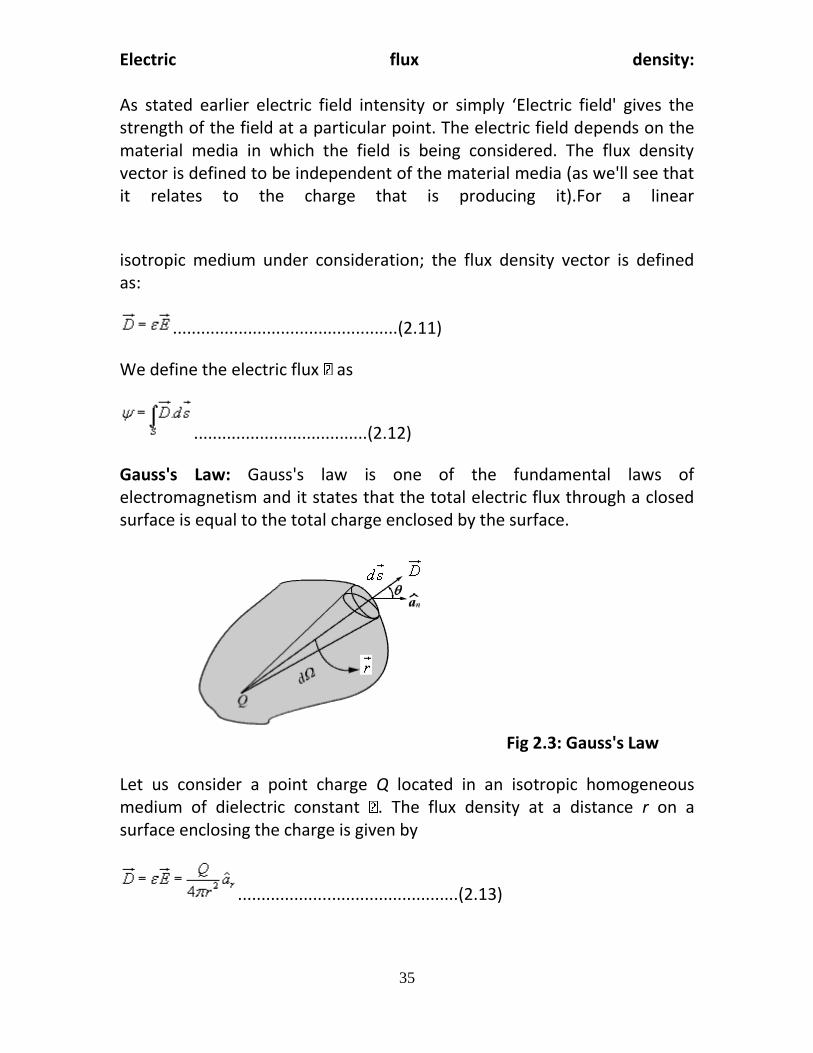
Gauss's Law: Gauss's law is one of the fundamental laws of electromagnetism and it states that the total electric flux through a closed surface is equal to the total charge enclosed by the surface.

Fig 2.3: Gauss's Law

Let us consider a point charge Q located in an isotropic homogeneous medium of dielectric constant . The flux density at a distance r on a surface enclosing the charge is given by

...............................................(2.13)

36

If we consider an elementary area ds, the amount of flux passing through the elementary area is given by

.....................................(2.14)

But , is the elementary solid angle subtended by the area at

the location of Q. Therefore we can write

For a closed surface enclosing the charge, we can write

which can seen to be same as what we have stated in the definition of Gauss's Law.

Application of Gauss's Law

Gauss's law is particularly useful in computing or where the charge distribution has some symmetry. We shall illustrate the application of Gauss's Law with some examples.

1.An infinite line charge

As the first example of illustration of use of Gauss's law, let consider the problem of determination of the electric field produced by an infinite line charge of density LC/m. Let us consider a line charge positioned along the z-axis as shown in Fig. 2.4(a) (next slide). Since the line charge is assumed to be infinitely long, the electric field will be of the form as shown in Fig. 2.4(b) (next slide).

If we consider a close cylindrical surface as shown in Fig. 2.4(a), using Gauss's theorm we can write,

.....................................(2.15)

Considering the fact that the unit normal vector to areas S1 and S3 are perpendicular to the electric field, the surface integrals for the top and

bottom surfaces evaluates to zero. Hence we can write,

37

Fig 2.4: Infinite Line Charge

.....................................(2.16)

2. Infinite Sheet of Charge

As a second example of application of Gauss's theorem, we consider an infinite charged sheet covering the x-z plane as shown in figure 2.5.

Assuming a surface charge density of for the infinite surface charge, if we consider a cylindrical volume having sides placed symmetrically as shown in figure 5, we can write:

38

..............(2.17)

Fig 2.5: Infinite Sheet of Charge

It may be noted that the electric field strength is independent of distance. This is true for the infinite plane of charge; electric lines of force on either side of the charge will be perpendicular to the sheet and extend to infinity as parallel lines. As number of lines of force per unit area gives the strength of the field, the field becomes independent of distance. For a finite charge sheet, the field will be a function of distance.

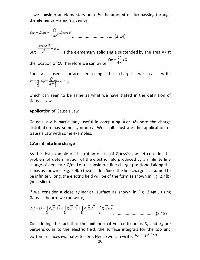
3. Uniformly Charged Sphere

Let us consider a sphere of radius r0 having a uniform volume charge

density of v C/m3. To determine everywhere, inside and outside the sphere, we construct Gaussian surfaces of radius r < r0 and r > r0 as shown in Fig. 2.6 (a) and Fig. 2.6(b).

For the region ; the total enclosed charge will be

.........................(2.18)

39

Fig 2.6: Uniformly Charged Sphere

By applying Gauss's theorem,

...............(2.19)

Therefore

...............................................(2.20)

For the region ; the total enclosed charge will be

....................................................................(2.21)

By applying Gauss's theorem,

.....................................................(2.22)

Electrostatic Potential and Equipotential Surfaces

In the previous sections we have seen how the electric field intensity due to a charge or a charge distribution can be found using Coulomb's law or Gauss's law. Since a charge placed in the vicinity of another charge (or in other words in the field of other charge) experiences a force, the movement of the charge represents energy exchange. Electrostatic

40

potential is related to the work done in carrying a charge from one point to the other in the presence of an electric field.

Let us suppose that we wish to move a positive test charge from a point P to another point Q as shown in the Fig. 2.8.

The force at any point along its path would cause the particle to accelerate and move it out of the region if unconstrained. Since we are dealing with an electrostatic case, a force equal to the negative of that acting on the charge

is to be applied while moves from P to Q. The work done by this external

agent in moving the charge by a distance is given by:

.............................(2.23)

Fig 2.8: Movement of Test Charge in Electric Field

The negative sign accounts for the fact that work is done on the system by the external agent.

.....................................(2.24)

The potential difference between two points P and Q , VPQ, is defined as the work done per unit charge, i.e.

...............................(2.25)

41

It may be noted that in moving a charge from the initial point to the final point if the potential difference is positive, there is a gain in potential energy in the movement, external agent performs the work against the field. If the sign of the potential difference is negative, work is done by the field.

We will see that the electrostatic system is conservative in that no net energy is exchanged if the test charge is moved about a closed path, i.e. returning to its initial position. Further, the potential difference between two points in an electrostatic field is a point function; it is independent of the path taken. The potential difference is measured in Joules/Coulomb which is referred to as Volts.

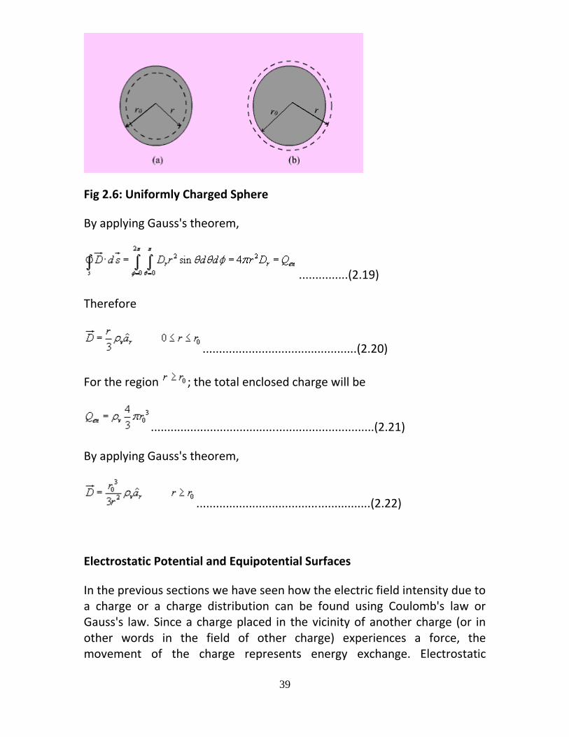
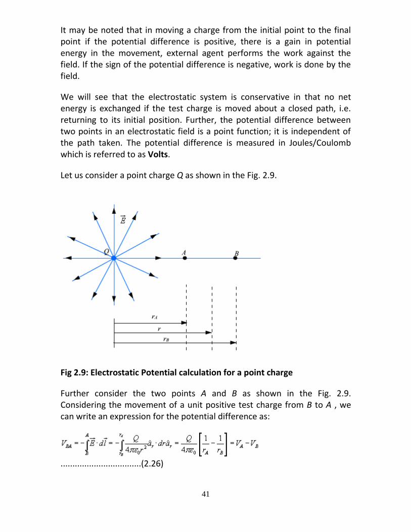
Let us consider a point charge Q as shown in the Fig. 2.9.

Fig 2.9: Electrostatic Potential calculation for a point charge

Further consider the two points A and B as shown in the Fig. 2.9. Considering the movement of a unit positive test charge from B to A , we can write an expression for the potential difference as:

..................................(2.26)

42

It is customary to choose the potential to be zero at infinity. Thus potential at any point ( rA = r) due to a point charge Q can be written as the amount of work done in bringing a unit positive charge from infinity to that point (i.e. rB = 0).

..................................(2.27)

Or, in other words,

..................................(2.28)

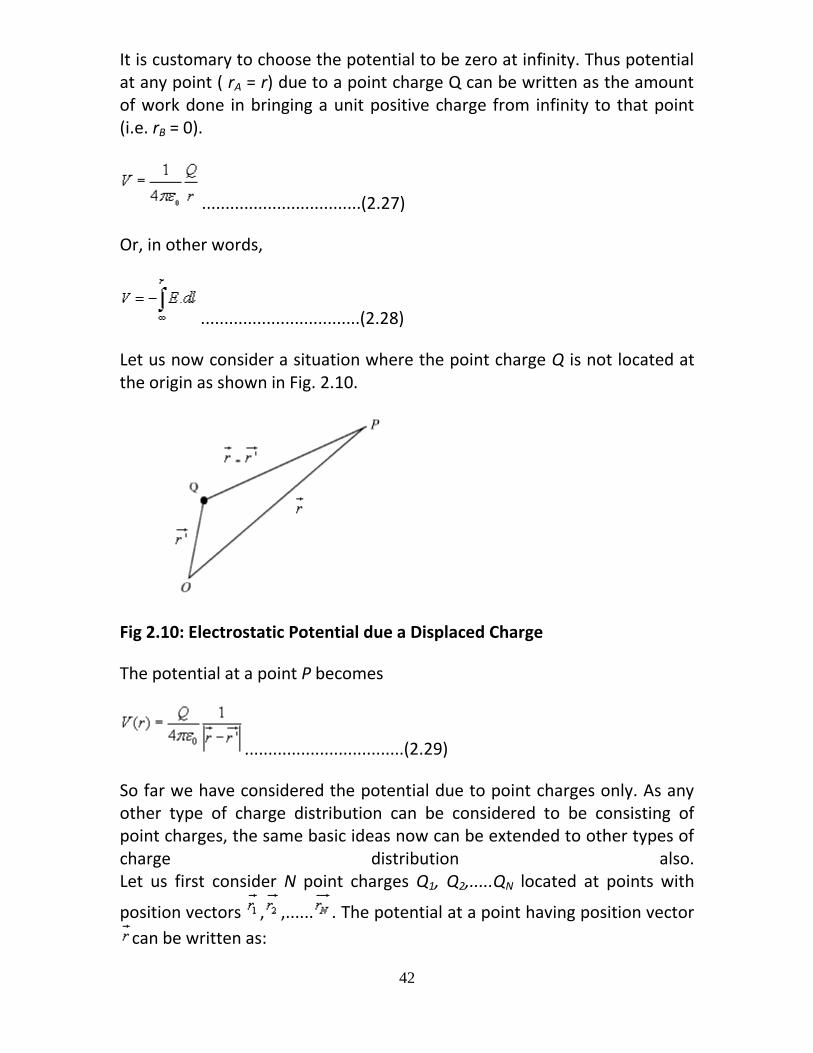
Let us now consider a situation where the point charge Q is not located at the origin as shown in Fig. 2.10.

Fig 2.10: Electrostatic Potential due a Displaced Charge

The potential at a point P becomes

..................................(2.29)

So far we have considered the potential due to point charges only. As any other type of charge distribution can be considered to be consisting of point charges, the same basic ideas now can be extended to other types of charge distribution also. Let us first consider N point charges Q1, Q2,.....QN located at points with

position vectors , ,...... . The potential at a point having position vector

can be written as:

43

..................................(2.30a)

or, ...........................................................(2.30b)

For continuous charge distribution, we replace point charges Qn by

corresponding charge elements or or depending on whether the charge distribution is linear, surface or a volume charge distribution and the summation is replaced by an integral. With these modifications we can write:

For line charge, ..................................(2.31)

For surface charge, .................................(2.32)

For volume charge, .................................(2.33)

It may be noted here that the primed coordinates represent the source coordinates and the unprimed coordinates represent field point.

Further, in our discussion so far we have used the reference or zero potential at infinity. If any other point is chosen as reference, we can write:

.................................(2.34)

where C is a constant. In the same manner when potential is computed from a known electric field we can write:

.................................(2.35)

The potential difference is however independent of the choice of reference.

44

.......................(2.36)

We have mentioned that electrostatic field is a conservative field; the work done in moving a charge from one point to the other is independent of the path. Let us consider moving a charge from point P1 to P2 in one path and then from point P2 back to P1 over a different path. If the work done on the two paths were different, a net positive or negative amount of work would have been done when the body returns to its original position P1. In a conservative field there is no mechanism for dissipating energy corresponding to any positive work neither any source is present from which energy could be absorbed in the case of negative work. Hence the question of different works in two paths is untenable, the work must have to be independent of path and depends on the initial and final positions.

Since the potential difference is independent of the paths taken, VAB = - VBA , and over a closed path,

.................................(2.37)

Applying Stokes's theorem, we can write:

............................(2.38)

from which it follows that for electrostatic field,

........................................(2.39)

Any vector field that satisfies is called an irrotational field.

From our definition of potential, we can write

.................................(2.40)

45

from which we obtain,

..........................................(2.41)

From the foregoing discussions we observe that the electric field strength at any point is the negative of the potential gradient at any point, negative

sign shows that is directed from higher to lower values of . This gives us another method of computing the electric field, i. e. if we know the potential function, the electric field may be computed. We may note here

that that one scalar function contain all the information that three

components of carry, the same is possible because of the fact that three

components of are interrelated by the relation .

Example: Electric Dipole

An electric dipole consists of two point charges of equal magnitude but of opposite sign and separated by a small distance.

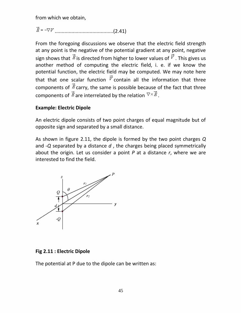
As shown in figure 2.11, the dipole is formed by the two point charges Q and -Q separated by a distance d , the charges being placed symmetrically about the origin. Let us consider a point P at a distance r, where we are interested to find the field.

Fig 2.11 : Electric Dipole

The potential at P due to the dipole can be written as:

46

..........................(2.42)

When r1 and r2>>d, we can write and .

Therefore,

....................................................(2.43)

We can write,

...............................................(2.44)

The quantity is called the dipole moment of the electric dipole.

Hence the expression for the electric potential can now be written as:

................................(2.45)

It may be noted that while potential of an isolated charge varies with distance as 1/r that of an electric dipole varies as 1/r2 with distance.

If the dipole is not centered at the origin, but the dipole center lies at , the expression for the potential can be written as:

........................(2.46)

The electric field for the dipole centered at the origin can be computed as

47

........................(2.47)

is the magnitude of the dipole moment. Once again we note that the electric field of electric dipole varies as 1/r3 where as that of a point charge varies as 1/r2.

Equipotential Surfaces

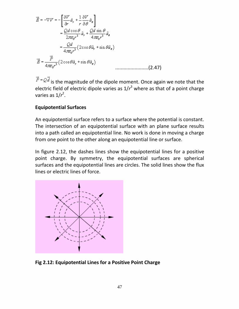
An equipotential surface refers to a surface where the potential is constant. The intersection of an equipotential surface with an plane surface results into a path called an equipotential line. No work is done in moving a charge from one point to the other along an equipotential line or surface.

In figure 2.12, the dashes lines show the equipotential lines for a positive point charge. By symmetry, the equipotential surfaces are spherical surfaces and the equipotential lines are circles. The solid lines show the flux lines or electric lines of force.

Fig 2.12: Equipotential Lines for a Positive Point Charge

48

Michael Faraday as a way of visualizing electric fields introduced flux lines. It may be seen that the electric flux lines and the equipotential lines are normal to each other.

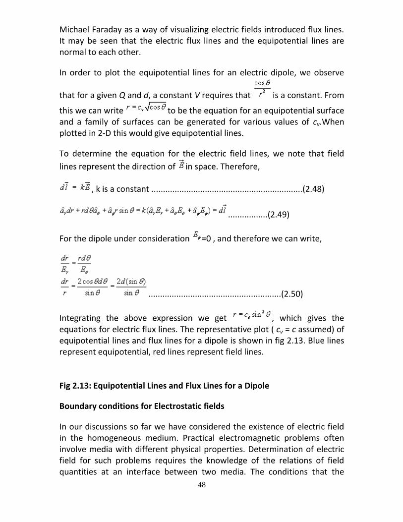
In order to plot the equipotential lines for an electric dipole, we observe

that for a given Q and d, a constant V requires that is a constant. From

this we can write to be the equation for an equipotential surface and a family of surfaces can be generated for various values of cv.When plotted in 2-D this would give equipotential lines.

To determine the equation for the electric field lines, we note that field

lines represent the direction of in space. Therefore,

, k is a constant .................................................................(2.48)

.................(2.49)

For the dipole under consideration =0 , and therefore we can write,

.........................................................(2.50)

Integrating the above expression we get , which gives the equations for electric flux lines. The representative plot ( cv = c assumed) of equipotential lines and flux lines for a dipole is shown in fig 2.13. Blue lines represent equipotential, red lines represent field lines. Fig 2.13: Equipotential Lines and Flux Lines for a Dipole

Boundary conditions for Electrostatic fields

In our discussions so far we have considered the existence of electric field in the homogeneous medium. Practical electromagnetic problems often involve media with different physical properties. Determination of electric field for such problems requires the knowledge of the relations of field quantities at an interface between two media. The conditions that the

49

fields must satisfy at the interface of two different media are referred to as boundary conditions .

In order to discuss the boundary conditions, we first consider the field behavior in some common material media.

In general, based on the electric properties, materials can be classified into three categories: conductors, semiconductors and insulators (dielectrics). In conductor , electrons in the outermost shells of the atoms are very loosely held and they migrate easily from one atom to the other. Most metals belong to this group. The electrons in the atoms of insulators or dielectrics remain confined to their orbits and under normal circumstances they are not liberated under the influence of an externally applied field. The electrical properties of semiconductors fall between those of conductors and insulators since semiconductors have very few numbers of free charges.

The parameter conductivity is used characterizes the macroscopic electrical property of a material medium. The notion of conductivity is more important in dealing with the current flow and hence the same will be considered in detail later on.

If some free charge is introduced inside a conductor, the charges will experience a force due to mutual repulsion and owing to the fact that they are free to move, the charges will appear on the surface. The charges will redistribute themselves in such a manner that the field within the conductor is zero. Therefore, under steady condition, inside a conductor

.

From Gauss's theorem it follows that

= 0 .......................(2.51)

The surface charge distribution on a conductor depends on the shape of the conductor. The charges on the surface of the conductor will not be in equilibrium if there is a tangential component of the electric field is present, which would produce movement of the charges. Hence under static field conditions, tangential component of the electric field on the conductor surface is zero. The electric field on the surface of the conductor is normal everywhere to the surface . Since the tangential component of electric field is zero, the conductor surface is an equipotential surface. As

50

= 0 inside the conductor, the conductor as a whole has the same potential. We may further note that charges require a finite time to

redistribute in a conductor. However, this time is very small sec for good conductor like copper.

Fig 2.14: Boundary Conditions for at the surface of a Conductor Let us now consider an interface between a conductor and free space as shown in the figure 2.14.Let us consider the closed path pqrsp for which we can write,

.................................(2.52)

For and noting that inside the conductor is zero, we can write

=0.......................................(2.53)

Et is the tangential component of the field. Therefore we find that

Et = 0 ...........................................(2.54)

In order to determine the normal component En, the normal component of

, at the surface of the conductor, we consider a small cylindrical Gaussian surface as shown in the Fig.12. Let represent the area of the top and bottom faces and represents the height of the cylinder. Once again, as

, we approach the surface of the conductor. Since = 0 inside the conductor is zero,

.............(2.55)

51

..................(2.56)

Therefore, we can summarize the boundary conditions at the surface of a conductor as:

Et = 0 ........................(2.57)

.....................(2.58)

Behavior of dielectrics in static electric field: Polarization of dielectric

Here we briefly describe the behavior of dielectrics or insulators when placed in static electric field. Ideal dielectrics do not contain free charges. As we know, all material media are composed of atoms where a positively charged nucleus (diameter ~ 10-15m) is surrounded by negatively charged electrons (electron cloud has radius ~ 10-10m) moving around the nucleus. Molecules of dielectrics are neutral macroscopically; an externally applied field causes small displacement of the charge particles creating small electric dipoles.These induced dipole moments modify electric fields both inside and outside dielectric material.

Molecules of some dielectric materials posses permanent dipole moments even in the absence of an external applied field. Usually such molecules consist of two or more dissimilar atoms and are called polar molecules. A common example of such molecule is water molecule H2O. In polar molecules the atoms do not arrange themselves to make the net dipole moment zero. However, in the absence of an external field, the molecules arrange themselves in a random manner so that net dipole moment over a volume becomes zero. Under the influence of an applied electric field, these dipoles tend to align themselves along the field as shown in figure 2.15. There are some materials that can exhibit net permanent dipole moment even in the absence of applied field. These materials are called electrets that made by heating certain waxes or plastics in the presence of electric field. The applied field aligns the polarized molecules when the material is in the heated state and they are frozen to their new position when after the temperature is brought down to its normal temperatures. Permanent polarization remains without an externally applied field.

52

As a measure of intensity of polarization, polarization vector (in C/m2) is

defined as: .......................(2.59)

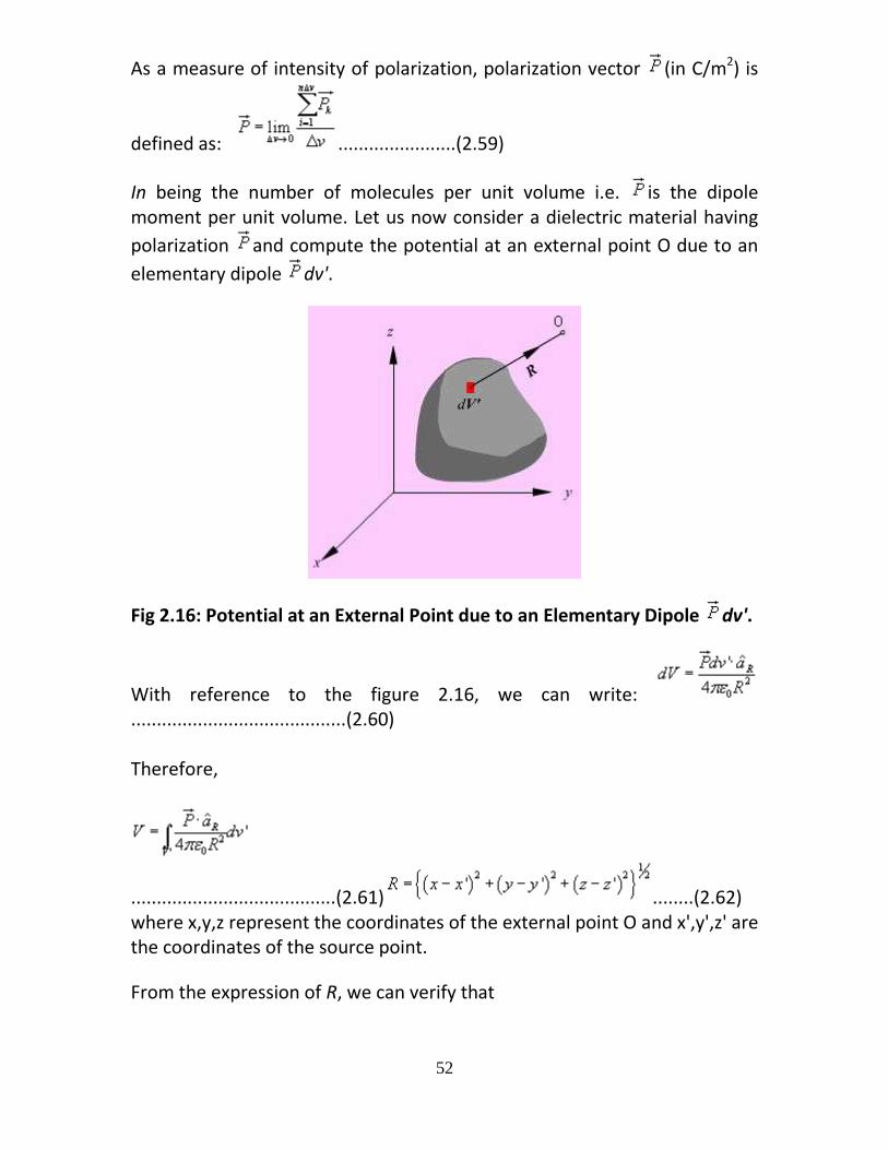
In being the number of molecules per unit volume i.e. is the dipole moment per unit volume. Let us now consider a dielectric material having

polarization and compute the potential at an external point O due to an

elementary dipole dv'.

Fig 2.16: Potential at an External Point due to an Elementary Dipole dv'.

With reference to the figure 2.16, we can write: ..........................................(2.60) Therefore,

........................................(2.61) ........(2.62) where x,y,z represent the coordinates of the external point O and x',y',z' are the coordinates of the source point.

From the expression of R, we can verify that

53

.............................................(2.63)

.........................................(2.64)

Using the vector identity, ,where f is a scalar quantity , we have,

.......................(2.65)

Converting the first volume integral of the above expression to surface integral, we can write

.................(2.66)

where is the outward normal from the surface element ds' of the dielectric. From the above expression we find that the electric potential of a polarized dielectric may be found from the contribution of volume and surface charge distributions having densities

......................................................................(2.67)

......................(2.68)

These are referred to as polarisation or bound charge densities. Therefore we may replace a polarized dielectric by an equivalent polarization surface charge density and a polarization volume charge density. We recall that bound charges are those charges that are not free to move within the dielectric material, such charges are result of displacement that occurs on a molecular scale during polarization. The total bound charge on the surface is

......................(2.69)

The charge that remains inside the surface is

54

......................(2.70)

The total charge in the dielectric material is zero as

......................(2.71)

If we now consider that the dielectric region containing charge density the total volume charge density becomes

....................(2.72)

Since we have taken into account the effect of the bound charge density, we can write

....................(2.73)

Using the definition of we have

....................(2.74)

Therefore the electric flux density

When the dielectric properties of the medium are linear and isotropic, polarisation is directly proportional to the applied field strength and

........................(2.75)

is the electric susceptibility of the dielectric. Therefore,

.......................(2.76)

is called relative permeability or the dielectric constant of the

medium. is called the absolute permittivity.

A dielectric medium is said to be linear when is independent of and the

medium is homogeneous if is also independent of space coordinates. A

55

linear homogeneous and isotropic medium is called a simple medium and for such medium the relative permittivity is a constant.

Dielectric constant may be a function of space coordinates. For anistropic materials, the dielectric constant is different in different directions of the electric field, D and E are related by a permittivity tensor which may be written as:

.......................(2.77)

For crystals, the reference coordinates can be chosen along the principal axes, which make off diagonal elements of the permittivity matrix zero. Therefore, we have

.......................(2.78)

Media exhibiting such characteristics are called biaxial. Further, if then the medium is called uniaxial. It may be noted that for isotropic

media, .

Lossy dielectric materials are represented by a complex dielectric constant, the imaginary part of which provides the power loss in the medium and this is in general dependant on frequency.

Another phenomenon is of importance is dielectric breakdown. We observed that the applied electric field causes small displacement of bound charges in a dielectric material that results into polarization. Strong field can pull electrons completely out of the molecules. These electrons being accelerated under influence of electric field will collide with molecular lattice structure causing damage or distortion of material. For very strong fields, avalanche breakdown may also occur. The dielectric under such condition will become conducting.

The maximum electric field intensity a dielectric can withstand without breakdown is referred to as the dielectric strength of the material.

56

Boundary Conditions for Electrostatic Fields:

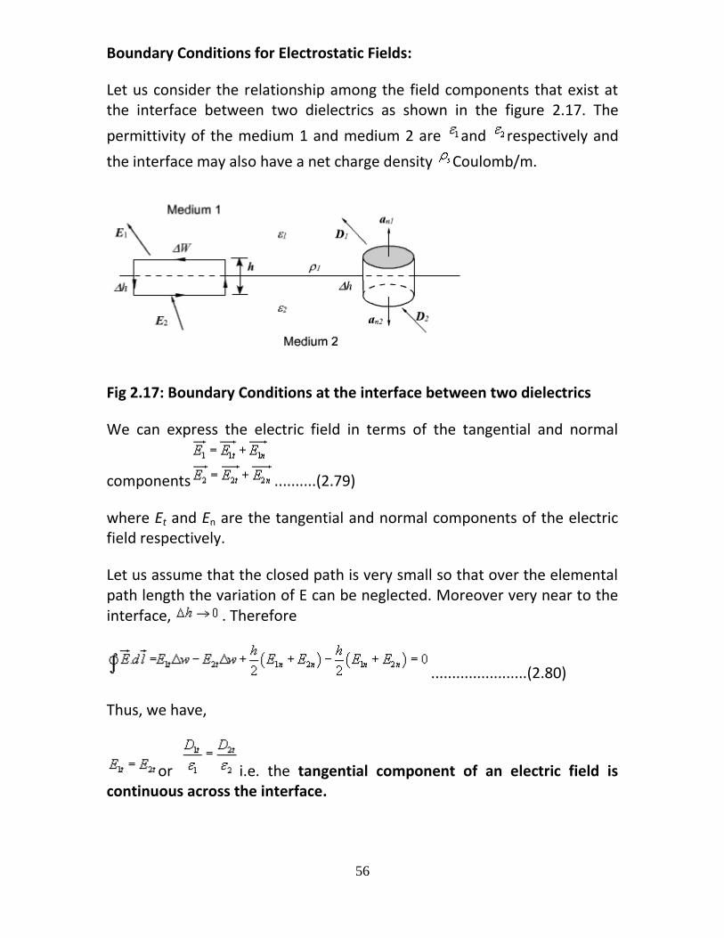
Let us consider the relationship among the field components that exist at the interface between two dielectrics as shown in the figure 2.17. The

permittivity of the medium 1 and medium 2 are and respectively and

the interface may also have a net charge density Coulomb/m.

Fig 2.17: Boundary Conditions at the interface between two dielectrics

We can express the electric field in terms of the tangential and normal

components ..........(2.79)

where Et and En are the tangential and normal components of the electric field respectively.

Let us assume that the closed path is very small so that over the elemental path length the variation of E can be neglected. Moreover very near to the interface, . Therefore

.......................(2.80)

Thus, we have,

or i.e. the tangential component of an electric field is continuous across the interface.

57

For relating the flux density vectors on two sides of the interface we apply Gauss’s law to a small pillbox volume as shown in the figure. Once again as

, we can write

..................(2.81a)

i.e., .................................................(2.81b)

.e., .......................(2.81c)

Thus we find that the normal component of the flux density vector D is discontinuous across an interface by an amount of discontinuity equal to the surface charge density at the interface.

Example

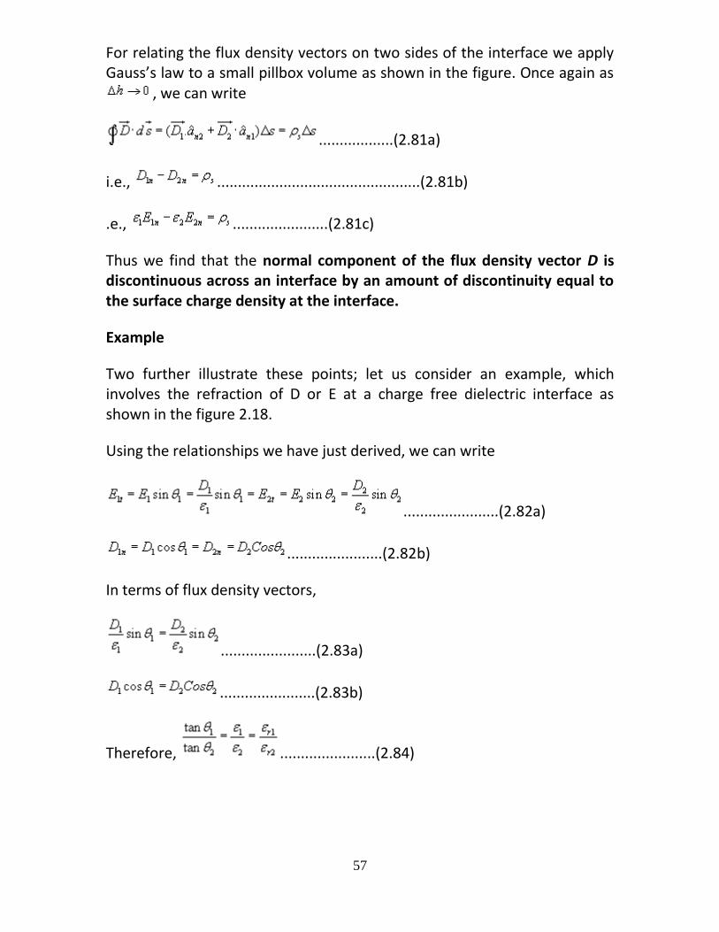
Two further illustrate these points; let us consider an example, which involves the refraction of D or E at a charge free dielectric interface as shown in the figure 2.18.

Using the relationships we have just derived, we can write

.......................(2.82a)

.......................(2.82b)

In terms of flux density vectors,

.......................(2.83a)

.......................(2.83b)

Therefore, .......................(2.84)

58

Fig 2.18: Refraction of D or E at a Charge Free Dielectric Interface

Capacitance and Capacitors

We have already stated that a conductor in an electrostatic field is an Equipotential body and any charge given to such conductor will distribute themselves in such a manner that electric field inside the conductor vanishes. If an additional amount of charge is supplied to an isolated conductor at a given potential, this additional charge will increase the

surface charge density . Since the potential of the conductor is given by

, the potential of the conductor will also increase

maintaining the ratio same. Thus we can write where the constant of proportionality C is called the capacitance of the isolated conductor. SI unit of capacitance is Coulomb/ Volt also called Farad denoted by F. It can It can be seen that if V=1, C = Q. Thus capacity of an isolated conductor can also be defined as the amount of charge in Coulomb required to raise the potential of the conductor by 1 Volt.

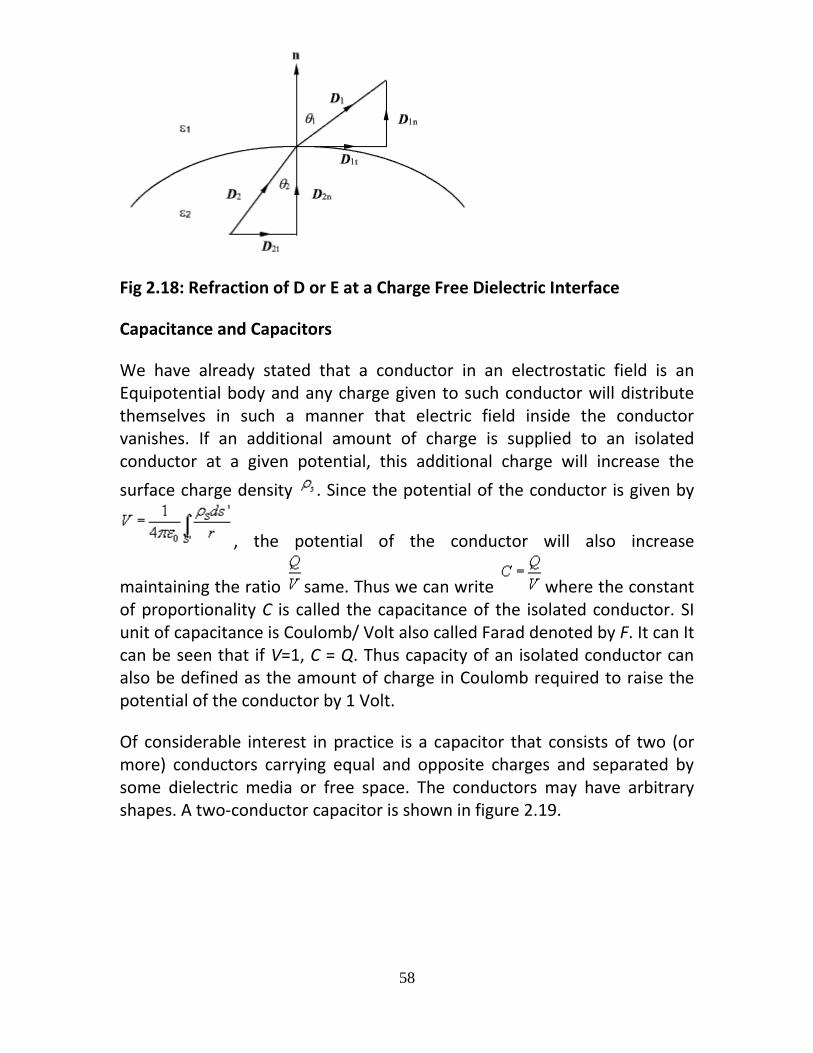
Of considerable interest in practice is a capacitor that consists of two (or more) conductors carrying equal and opposite charges and separated by some dielectric media or free space. The conductors may have arbitrary shapes. A two-conductor capacitor is shown in figure 2.19.

59

Fig 2.19: Capacitance and Capacitors

When a d-c voltage source is connected between the conductors, a charge transfer occurs which results into a positive charge on one conductor and negative charge on the other conductor. The conductors are equipotential surfaces and the field lines are perpendicular to the conductor surface. If V is the mean potential difference between the conductors, the capacitance

is given by . Capacitance of a capacitor depends on the geometry of the conductor and the permittivity of the medium between them and does not depend on the charge or potential difference between conductors. The capacitance can be computed by assuming Q(at the same time -Q on the

other conductor), first determining using Gauss’s theorem and then

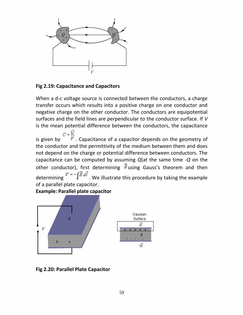
determining . We illustrate this procedure by taking the example of a parallel plate capacitor. Example: Parallel plate capacitor

Fig 2.20: Parallel Plate Capacitor

60

For the parallel plate capacitor shown in the figure 2.20, let each plate has area A and a distance h separates the plates. A dielectric of permittivity fills the region between the plates. The electric field lines are confined between the plates. We ignore the flux fringing at the edges of the plates and charges are assumed to be uniformly distributed over the conducting

plates with densities and - , .

By Gauss’s theorem we can write, .......................(2.85)

As we have assumed to be uniform and fringing of field is neglected, we see that E is constant in the region between the plates and therefore, we

can write . Thus, for a parallel plate capacitor we have,

........................(2.86)

Series and parallel Connection of capacitors

Capacitors are connected in various manners in electrical circuits; series and parallel connections are the two basic ways of connecting capacitors. We compute the equivalent capacitance for such connections.

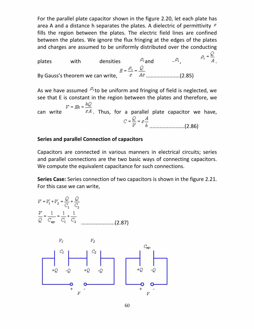
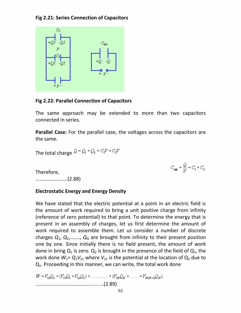
Series Case: Series connection of two capacitors is shown in the figure 2.21. For this case we can write,

.......................(2.87)

61

Fig 2.21: Series Connection of Capacitors

Fig 2.22: Parallel Connection of Capacitors

The same approach may be extended to more than two capacitors connected in series.

Parallel Case: For the parallel case, the voltages across the capacitors are the same.

The total charge

Therefore, .......................(2.88)

Electrostatic Energy and Energy Density

We have stated that the electric potential at a point in an electric field is the amount of work required to bring a unit positive charge from infinity (reference of zero potential) to that point. To determine the energy that is present in an assembly of charges, let us first determine the amount of work required to assemble them. Let us consider a number of discrete charges Q1, Q2,......., QN are brought from infinity to their present position one by one. Since initially there is no field present, the amount of work done in bring Q1 is zero. Q2 is brought in the presence of the field of Q1, the work done W1= Q2V21 where V21 is the potential at the location of Q2 due to Q1. Proceeding in this manner, we can write, the total work done

.................................................(2.89)

62

Had the charges been brought in the reverse order,

.................(2.90)

Therefore,

................(2.91)

Here VIJ represent voltage at the Ith charge location due to Jth charge. Therefore,

Or, ................(2.92)

If instead of discrete charges, we now have a distribution of charges over a volume v then we can write,

................(2.93)

where is the volume charge density and V represents the potential function.

Since, , we can write

.......................................(2.94)

Using the vector identity,

, we can write

63

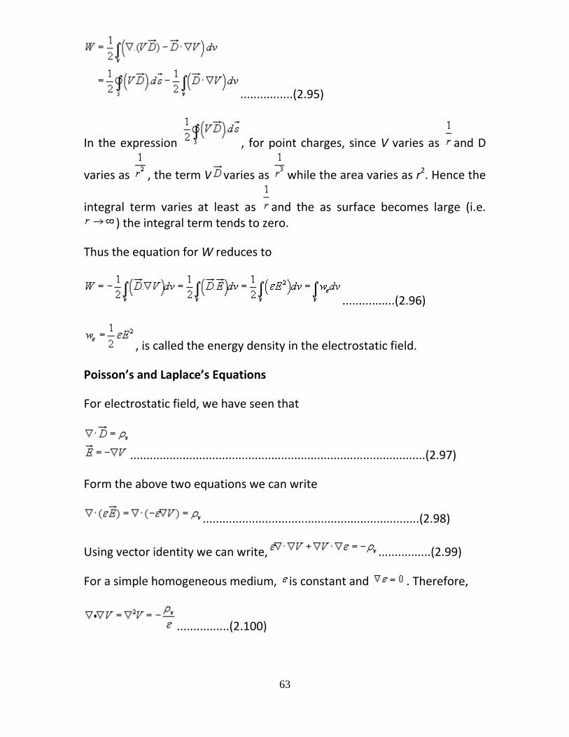
................(2.95)

In the expression , for point charges, since V varies as and D

varies as , the term V varies as while the area varies as r2. Hence the

integral term varies at least as and the as surface becomes large (i.e. ) the integral term tends to zero.

Thus the equation for W reduces to

................(2.96)

, is called the energy density in the electrostatic field.

Poisson’s and Laplace’s Equations

For electrostatic field, we have seen that

..........................................................................................(2.97)

Form the above two equations we can write

..................................................................(2.98)

Using vector identity we can write, ................(2.99)

For a simple homogeneous medium, is constant and . Therefore,

................(2.100)

64

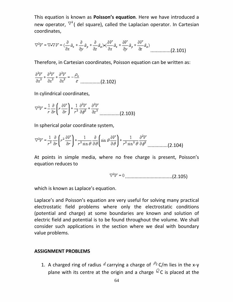
This equation is known as Poisson’s equation. Here we have introduced a

new operator, ( del square), called the Laplacian operator. In Cartesian coordinates,

...............(2.101)

Therefore, in Cartesian coordinates, Poisson equation can be written as:

...............(2.102)

In cylindrical coordinates,

...............(2.103)

In spherical polar coordinate system,

...............(2.104)

At points in simple media, where no free charge is present, Poisson’s equation reduces to

...................................(2.105)

which is known as Laplace’s equation.

Laplace’s and Poisson’s equation are very useful for solving many practical electrostatic field problems where only the electrostatic conditions (potential and charge) at some boundaries are known and solution of electric field and potential is to be found throughout the volume. We shall consider such applications in the section where we deal with boundary value problems.

ASSIGNMENT PROBLEMS

1. A charged ring of radius carrying a charge of C/m lies in the x-y

plane with its centre at the origin and a charge C is placed at the

65

point . Determine in terms of and so that a test charge

placed at does not experience any force.

2. A semicircular ring of radius lies in the free space and carries a

charge density C/m. Find the electric field at the centre of the semicircle.

3. Consider a uniform sphere of charge with charge density and radius b , centered at the origin. Find the electric field at a distance r from the origin for the two cases: r<b and r>b . Sketch the strength of the electric filed as function of r .

4. A spherical charge distribution is given by

is the radius of the sphere. Find the following:

i. The total charge.

ii. for and .

iii. The value of where the becomes maximum.

5. With reference to the Figure 2.6 determine the potential and field at

the point if the shaded region contains uniform charge

density /m2 .

FIgure 2.6

6. A capacitor consists of two coaxial metallic cylinders of length , radius of the inner conductor and that of outer conductor . A

66

dielectric material having dielectric constant , where is the radius, fills the space between the conductors. Determine the capacitance of the capacitor.

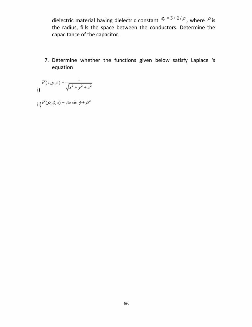
7. Determine whether the functions given below satisfy Laplace 's equation

i)

ii)

67

Unit III Magnetostatics

In previous chapters we have seen that an electrostatic field is produced by static or stationary charges. The relationship of the steady magnetic field to its sources is much more complicated.

The source of steady magnetic field may be a permanent magnet, a direct current or an electric field changing with time. In this chapter we shall mainly consider the magnetic field produced by a direct current. The magnetic field produced due to time varying electric field will be discussed later. Historically, the link between the electric and magnetic field was established Oersted in 1820. Ampere and others extended the investigation of magnetic effect of electricity . There are two major laws governing the magnetostatic fields are:

Biot-Savart Law Ampere's Law

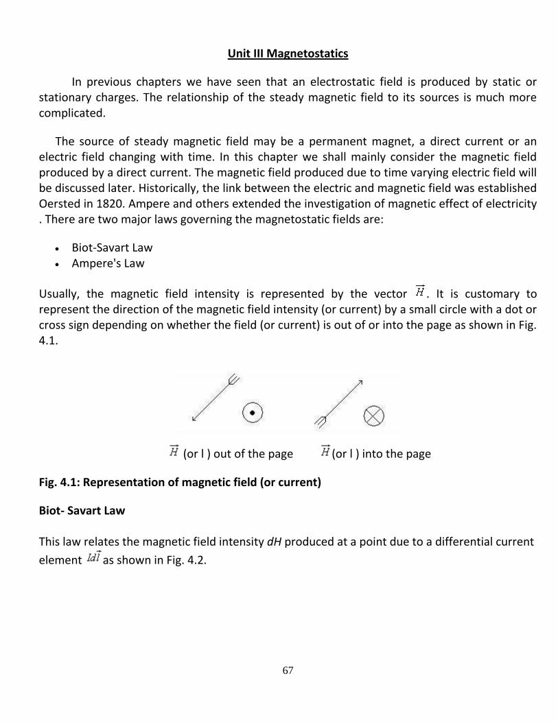
Usually, the magnetic field intensity is represented by the vector . It is customary to represent the direction of the magnetic field intensity (or current) by a small circle with a dot or cross sign depending on whether the field (or current) is out of or into the page as shown in Fig. 4.1.

(or l ) out of the page (or l ) into the page

Fig. 4.1: Representation of magnetic field (or current)

Biot- Savart Law This law relates the magnetic field intensity dH produced at a point due to a differential current

element as shown in Fig. 4.2.

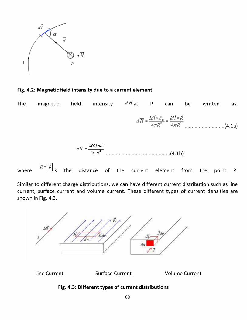
68

Fig. 4.2: Magnetic field intensity due to a current element

The magnetic field intensity at P can be written as,

............................(4.1a)

..............................................(4.1b)

where is the distance of the current element from the point P. Similar to different charge distributions, we can have different current distribution such as line current, surface current and volume current. These different types of current densities are shown in Fig. 4.3.

Line Current Surface Current Volume Current Fig. 4.3: Different types of current distributions

69

By denoting the surface current density as K (in amp/m) and volume current density as J (in amp/m2) we can write:

......................................(4.2)

( It may be noted that )

Employing Biot-Savart Law, we can now express the magnetic field intensity H. In terms of these current distributions.

............................. for line current............................(4.3a)

........................ for surface current ....................(4.3b)

....................... for volume current......................(4.3c) To illustrate the application of Biot - Savart's Law, we consider the following example.

Example 4.1: We consider a finite length of a conductor carrying a current placed along z-axis as shown in the Fig 4.4. We determine the magnetic field at point P due to this current carrying conductor.

Fig. 4.4: Field at a point P due to a finite length current carrying conductor

70

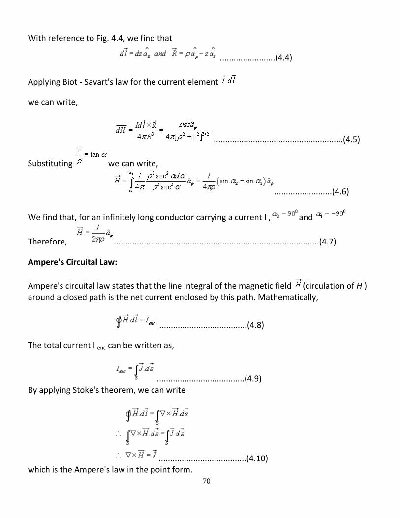
With reference to Fig. 4.4, we find that

........................(4.4)

Applying Biot - Savart's law for the current element

we can write,

........................................................(4.5)

Substituting we can write,

.........................(4.6)

We find that, for an infinitely long conductor carrying a current I , and

Therefore, .........................................................................................(4.7)

Ampere's Circuital Law:

Ampere's circuital law states that the line integral of the magnetic field (circulation of H ) around a closed path is the net current enclosed by this path. Mathematically,

......................................(4.8)

The total current I enc can be written as,

......................................(4.9) By applying Stoke's theorem, we can write

......................................(4.10) which is the Ampere's law in the point form.

71

Applications of Ampere's law: We illustrate the application of Ampere's Law with some examples.

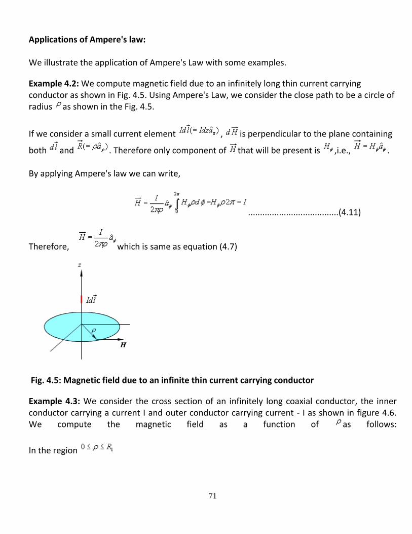
Example 4.2: We compute magnetic field due to an infinitely long thin current carrying conductor as shown in Fig. 4.5. Using Ampere's Law, we consider the close path to be a circle of radius as shown in the Fig. 4.5.

If we consider a small current element , is perpendicular to the plane containing

both and . Therefore only component of that will be present is ,i.e., . By applying Ampere's law we can write,

......................................(4.11)

Therefore, which is same as equation (4.7)

Fig. 4.5: Magnetic field due to an infinite thin current carrying conductor

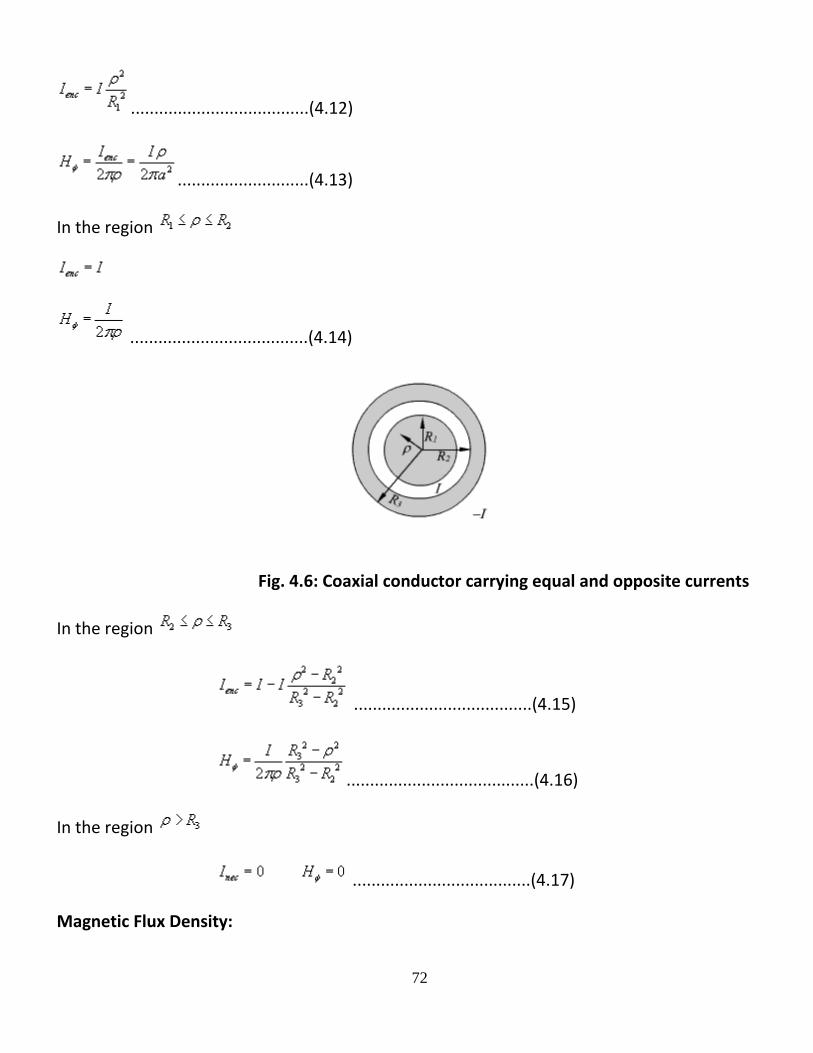
Example 4.3: We consider the cross section of an infinitely long coaxial conductor, the inner conductor carrying a current I and outer conductor carrying current - I as shown in figure 4.6. We compute the magnetic field as a function of as follows:

In the region

72

......................................(4.12)

............................(4.13)

In the region

......................................(4.14)

Fig. 4.6: Coaxial conductor carrying equal and opposite currents

In the region

......................................(4.15)

........................................(4.16)

In the region

......................................(4.17)

Magnetic Flux Density:

73

In simple matter, the magnetic flux density related to the magnetic field intensity as

where called the permeability. In particular when we consider the free space

where H/m is the permeability of the free space. Magnetic flux density is measured in terms of Wb/m 2 .

The magnetic flux density through a surface is given by:

Wb ......................................(4.18)

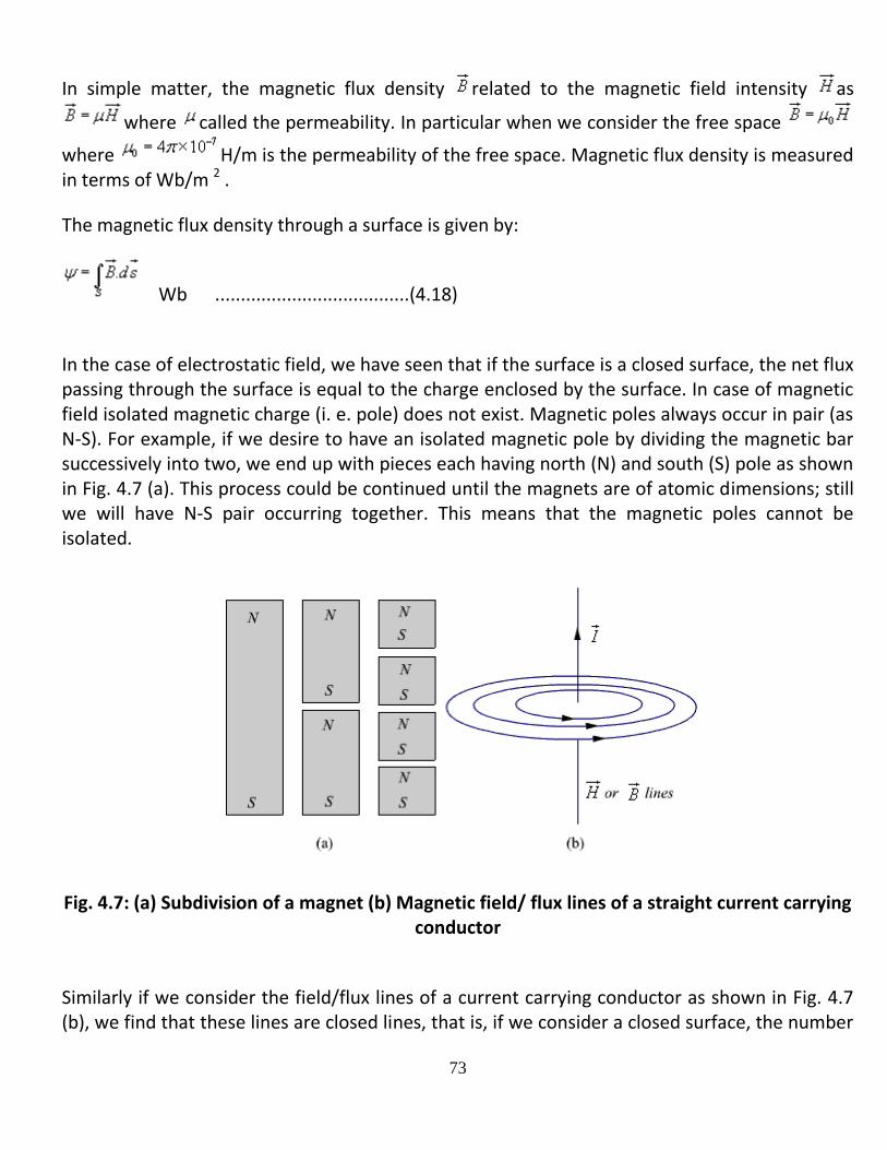
In the case of electrostatic field, we have seen that if the surface is a closed surface, the net flux passing through the surface is equal to the charge enclosed by the surface. In case of magnetic field isolated magnetic charge (i. e. pole) does not exist. Magnetic poles always occur in pair (as N-S). For example, if we desire to have an isolated magnetic pole by dividing the magnetic bar successively into two, we end up with pieces each having north (N) and south (S) pole as shown in Fig. 4.7 (a). This process could be continued until the magnets are of atomic dimensions; still we will have N-S pair occurring together. This means that the magnetic poles cannot be isolated.

Fig. 4.7: (a) Subdivision of a magnet (b) Magnetic field/ flux lines of a straight current carrying conductor

Similarly if we consider the field/flux lines of a current carrying conductor as shown in Fig. 4.7 (b), we find that these lines are closed lines, that is, if we consider a closed surface, the number

74

of flux lines that would leave the surface would be same as the number of flux lines that would enter the surface. From our discussions above, it is evident that for magnetic field,

......................................(4.19)

which is the Gauss's law for the magnetic field. By applying divergence theorem, we can write:

Hence, ......................................(4.20)

which is the Gauss's law for the magnetic field in point form.

Magnetic Scalar and Vector Potentials:

In studying electric field problems, we introduced the concept of electric potential that simplified the computation of electric fields for certain types of problems. In the same manner let us relate the magnetic field intensity to a scalar magnetic potential and write:

...................................(4.21)

From Ampere's law , we know that

......................................(4.22)

Therefore, ............................(4.23)

But using vector identity, we find that is valid only where . Thus the

scalar magnetic potential is defined only in the region where . Moreover, Vm in general is not a single valued function of position.

75

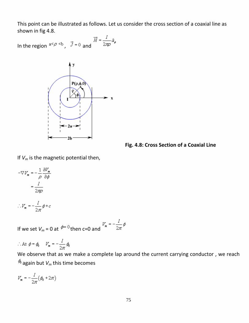
This point can be illustrated as follows. Let us consider the cross section of a coaxial line as shown in fig 4.8.

In the region , and

Fig. 4.8: Cross Section of a Coaxial Line

If Vm is the magnetic potential then,

If we set Vm = 0 at then c=0 and

We observe that as we make a complete lap around the current carrying conductor , we reach

again but Vm this time becomes

76

We observe that value of Vm keeps changing as we complete additional laps to pass through the same point. We introduced Vm analogous to electostatic potential V. But for static electric

fields, and , whereas for steady magnetic field wherever but

even if along the path of integration.

We now introduce the vector magnetic potential which can be used in regions where current density may be zero or nonzero and the same can be easily extended to time varying cases. The use of vector magnetic potential provides elegant ways of solving EM field problems.

Since and we have the vector identity that for any vector , , we can write

.

Here, the vector field is called the vector magnetic potential. Its SI unit is Wb/m. Thus if can

find of a given current distribution, can be found from through a curl operation.

We have introduced the vector function and related its curl to . A vector function is defined

fully in terms of its curl as well as divergence. The choice of is made as follows.

...........................................(4.24)

By using vector identity, .................................................(4.25)

.........................................(4.26)

Great deal of simplification can be achieved if we choose .

Putting , we get which is vector poisson equation. In Cartesian coordinates, the above equation can be written in terms of the components as

......................................(4.27a)

......................................(4.27b)

......................................(4.27c)

The form of all the above equation is same as that of

77

..........................................(4.28)

for which the solution is

..................(4.29)

In case of time varying fields we shall see that , which is known as Lorentz condition,

V being the electric potential. Here we are dealing with static magnetic field, so .

By comparison, we can write the solution for Ax as

...................................(4.30)

Computing similar solutions for other two components of the vector potential, the vector potential can be written as

.......................................(4.31)

This equation enables us to find the vector potential at a given point because of a volume

current density . Similarly for line or surface current density we can write

...................................................(4.32)

respectively. ..............................(4.33)

The magnetic flux through a given area S is given by

.............................................(4.34)

Substituting

78

.........................................(4.35)

Vector potential thus have the physical significance that its integral around any closed path is equal to the magnetic flux passing through that path.

Boundary Condition for Magnetic Fields:

Similar to the boundary conditions in the electro static fields, here we will consider the

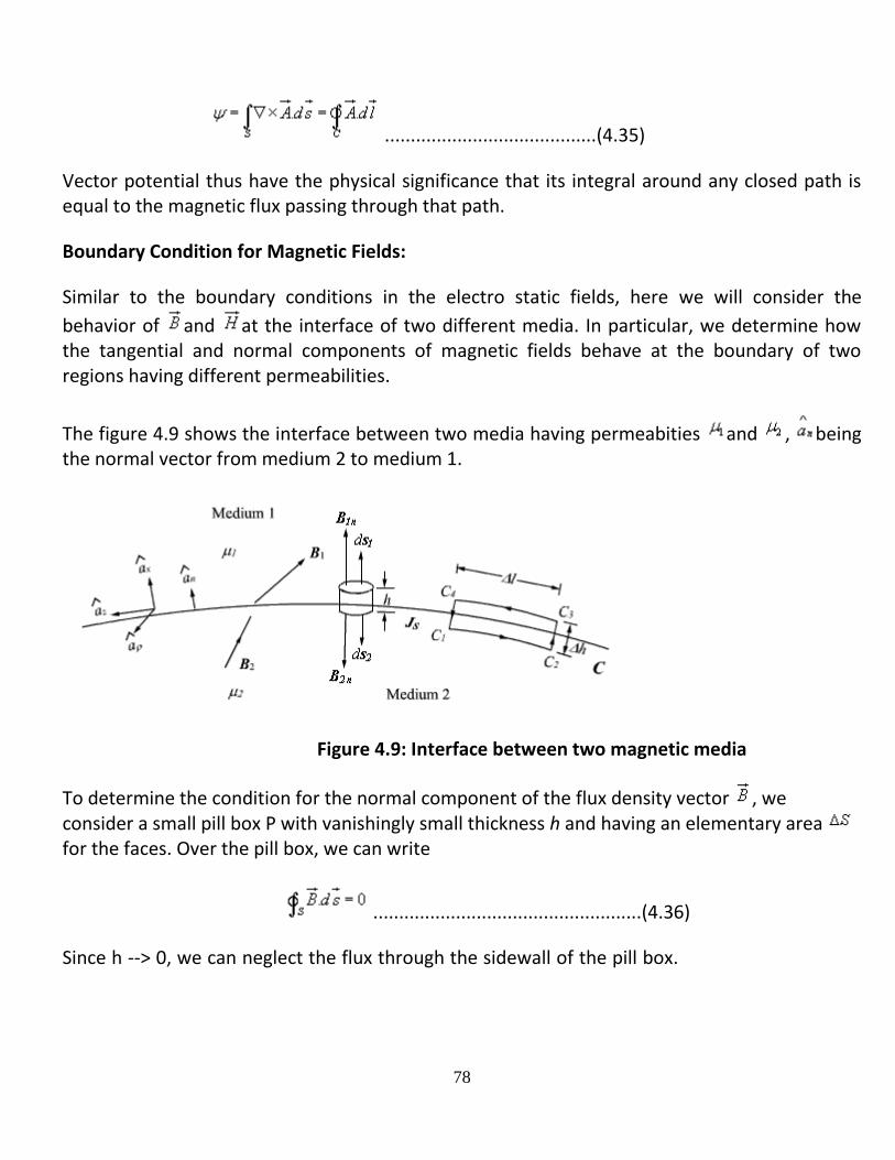
behavior of and at the interface of two different media. In particular, we determine how the tangential and normal components of magnetic fields behave at the boundary of two regions having different permeabilities.

The figure 4.9 shows the interface between two media having permeabities and , being the normal vector from medium 2 to medium 1.

Figure 4.9: Interface between two magnetic media

To determine the condition for the normal component of the flux density vector , we consider a small pill box P with vanishingly small thickness h and having an elementary area for the faces. Over the pill box, we can write

....................................................(4.36)

Since h --> 0, we can neglect the flux through the sidewall of the pill box.

79

...........................(4.37)

and ..................(4.38)

where

and ..........................(4.39)

Since is small, we can write

or, ...................................(4.40)

That is, the normal component of the magnetic flux density vector is continuous across the interface.

In vector form,

...........................(4.41) To determine the condition for the tangential component for the magnetic field, we consider a closed path C as shown in figure 4.8. By applying Ampere's law we can write

....................................(4.42)

Since h -->0,

...................................(4.43)

We have shown in figure 4.8, a set of three unit vectors , and such that they satisfy

(R.H. rule). Here is tangential to the interface and is the vector perpendicular to the surface enclosed by C at the interface

80

The above equation can be written as

or, ...................................(4.44) i.e., tangential component of magnetic field component is discontinuous across the interface where a free surface current exists.

If Js = 0, the tangential magnetic field is also continuous. If one of the medium is a perfect conductor Js exists on the surface of the perfect conductor.

In vector form we can write,

...................................(4.45)

Therefore,

...................................(4.46)

ASSIGNMENT PROBLEMS

1. An infinitely long conductor carries a current I A is bent into an L shape and placed as shown in Fig. P.4.7. Determine the magnetic field intensity at a point P (0,0, a).

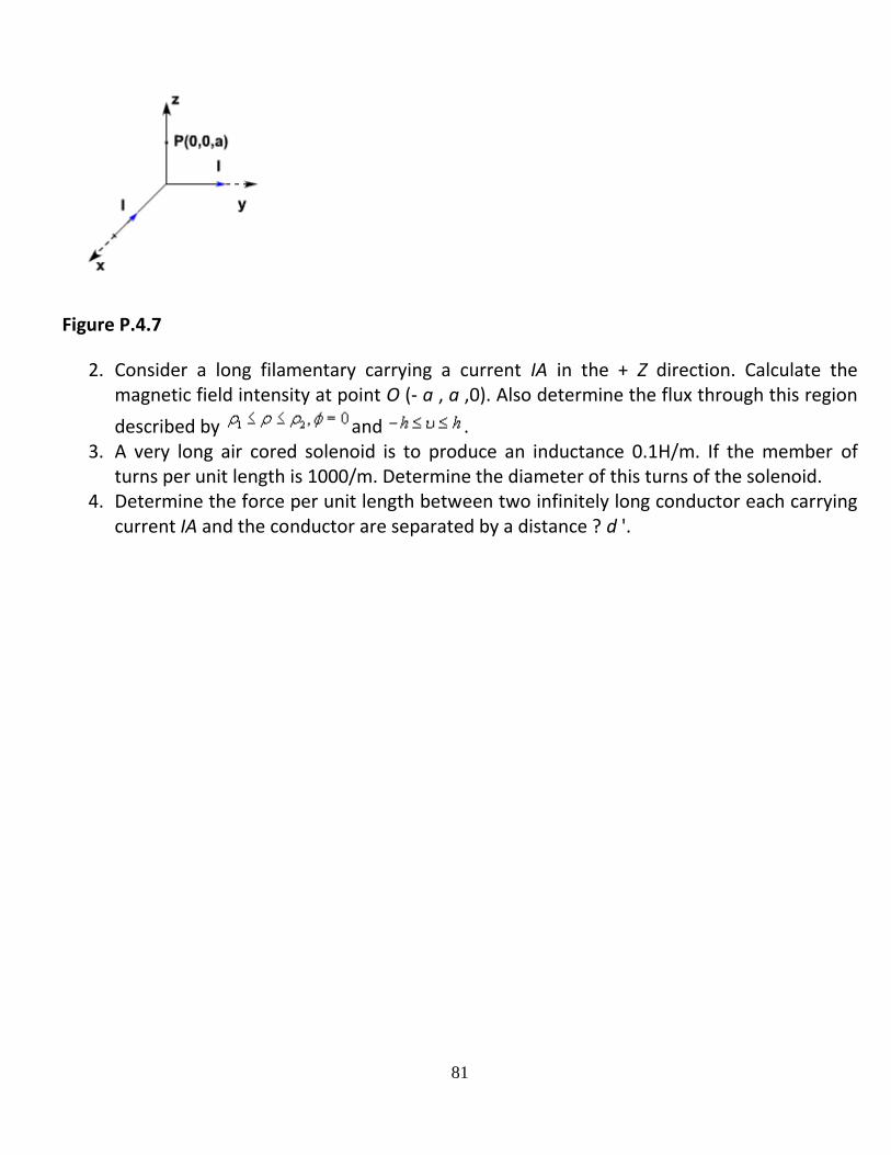
81

Figure P.4.7

2. Consider a long filamentary carrying a current IA in the + Z direction. Calculate the magnetic field intensity at point O (- a , a ,0). Also determine the flux through this region

described by and . 3. A very long air cored solenoid is to produce an inductance 0.1H/m. If the member of

turns per unit length is 1000/m. Determine the diameter of this turns of the solenoid. 4. Determine the force per unit length between two infinitely long conductor each carrying

current IA and the conductor are separated by a distance ? d '.

82

Unit IV Electrodynamic fields

Introduction: In our study of static fields so far, we have observed that static electric fields are produced by electric charges, static magnetic fields are produced by charges in motion or by steady current. Further, static electric field is a conservative field and has no curl, the static magnetic field is continuous and its divergence is zero. The fundamental relationships for static electric fields among the field quantities can be summarized as:

(5.1a)

(5.1b)

For a linear and isotropic medium,

(5.1c)

Similarly for the magnetostatic case

(5.2a)

(5.2b)

(5.2c)

It can be seen that for static case, the electric field vectors and and

magnetic field vectors and form separate pairs.

In this chapter we will consider the time varying scenario. In the time varying case we will observe that a changing magnetic field will produce a changing electric field and vice versa.

We begin our discussion with Faraday's Law of electromagnetic induction and then present the Maxwell's equations which form the foundation for the electromagnetic theory.

83

Faraday's Law of electromagnetic Induction

Michael Faraday, in 1831 discovered experimentally that a current was induced in a conducting loop when the magnetic flux linking the loop changed. In terms of fields, we can say that a time varying magnetic field produces an electromotive force (emf) which causes a current in a closed circuit. The quantitative relation between the induced emf (the voltage that arises from conductors moving in a magnetic field or from changing magnetic fields) and the rate of change of flux linkage developed based on experimental observation is known as Faraday's law. Mathematically, the induced emf can be written as

Emf = Volts (5.3)

where is the flux linkage over the closed path.

A non zero may result due to any of the following:

(a) time changing flux linkage a stationary closed path.

(b) relative motion between a steady flux a closed path.

(c) a combination of the above two cases.

The negative sign in equation (5.3) was introduced by Lenz in order to comply with the polarity of the induced emf. The negative sign implies that the induced emf will cause a current flow in the closed loop in such a direction so as to oppose the change in the linking magnetic flux which produces it. (It may be noted that as far as the induced emf is concerned, the closed path forming a loop does not necessarily have to be conductive).

If the closed path is in the form of N tightly wound turns of a coil, the change in the magnetic flux linking the coil induces an emf in each turn of the coil and total emf is the sum of the induced emfs of the individual turns, i.e.,

84

Emf = Volts (5.4)

By defining the total flux linkage as

(5.5)

The emf can be written as

Emf = (5.6)

Continuing with equation (5.3), over a closed contour 'C' we can write

Emf = (5.7)

where is the induced electric field on the conductor to sustain the current.

Further, total flux enclosed by the contour 'C ' is given by

(5.8)

Where S is the surface for which 'C' is the contour.

From (5.7) and using (5.8) in (5.3) we can write

(5.9)

By applying stokes theorem

(5.10)

Therefore, we can write

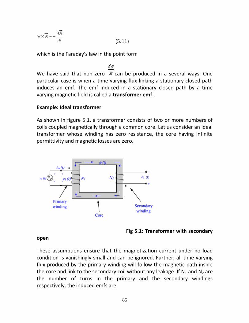
85

(5.11)

which is the Faraday's law in the point form

We have said that non zero can be produced in a several ways. One particular case is when a time varying flux linking a stationary closed path induces an emf. The emf induced in a stationary closed path by a time varying magnetic field is called a transformer emf .

Example: Ideal transformer

As shown in figure 5.1, a transformer consists of two or more numbers of coils coupled magnetically through a common core. Let us consider an ideal transformer whose winding has zero resistance, the core having infinite permittivity and magnetic losses are zero.

Fig 5.1: Transformer with secondary open

These assumptions ensure that the magnetization current under no load condition is vanishingly small and can be ignored. Further, all time varying flux produced by the primary winding will follow the magnetic path inside the core and link to the secondary coil without any leakage. If N1 and N2 are the number of turns in the primary and the secondary windings respectively, the induced emfs are

86

(5.12a)

(5.12b)

(The polarities are marked, hence negative sign is omitted. The induced emf is +ve at the dotted end of the winding.)

(5.13)

i.e., the ratio of the induced emfs in primary and secondary is equal to the ratio of their turns. Under ideal condition, the induced emf in either winding is equal to their voltage rating.

(5.14)

where 'a' is the transformation ratio. When the secondary winding is connected to a load, the current flows in the secondary, which produces a flux opposing the original flux. The net flux in the core decreases and induced emf will tend to decrease from the no load value. This causes the primary current to increase to nullify the decrease in the flux and induced emf. The current continues to increase till the flux in the core and the induced emfs are restored to the no load values. Thus the source supplies power to the primary winding and the secondary winding delivers the power to the load. Equating the powers

(5.15)

(5.16)

Further,

(5.17)

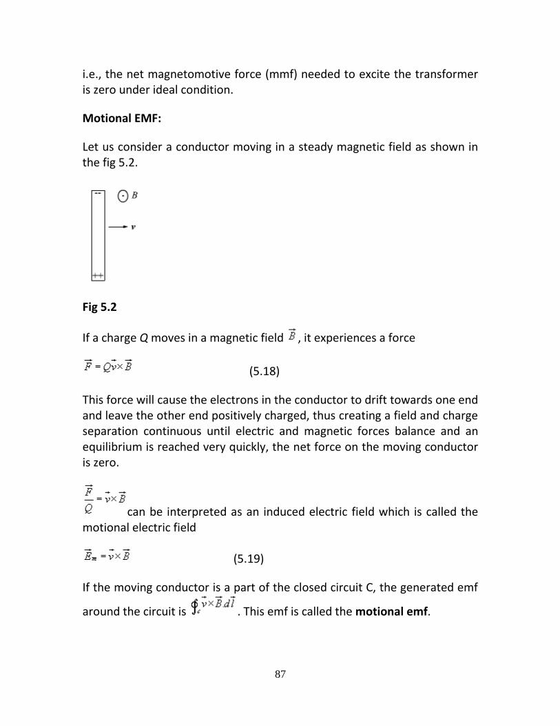
87

i.e., the net magnetomotive force (mmf) needed to excite the transformer is zero under ideal condition.

Motional EMF:

Let us consider a conductor moving in a steady magnetic field as shown in the fig 5.2.

Fig 5.2

If a charge Q moves in a magnetic field , it experiences a force

(5.18)

This force will cause the electrons in the conductor to drift towards one end and leave the other end positively charged, thus creating a field and charge separation continuous until electric and magnetic forces balance and an equilibrium is reached very quickly, the net force on the moving conductor is zero.

can be interpreted as an induced electric field which is called the motional electric field

(5.19)

If the moving conductor is a part of the closed circuit C, the generated emf

around the circuit is . This emf is called the motional emf.

88

A classic example of motional emf is given in Additonal Solved Example No.1 .

Maxwell's Equation

Equation (5.1) and (5.2) gives the relationship among the field quantities in the static field. For time varying case, the relationship among the field vectors written as

(5.20a)

(5.20b)

(5.20c)

(5.20d)

In addition, from the principle of conservation of charges we get the equation of continuity

(5.21) The equation 5.20 (a) - (d) must be consistent with equation (5.21).

We observe that

(5.22)

Since is zero for any vector .

Thus applies only for the static case i.e., for the scenario when

. A classic example for this is given below . Suppose we are in the process of charging up a capacitor as shown in fig 5.3.

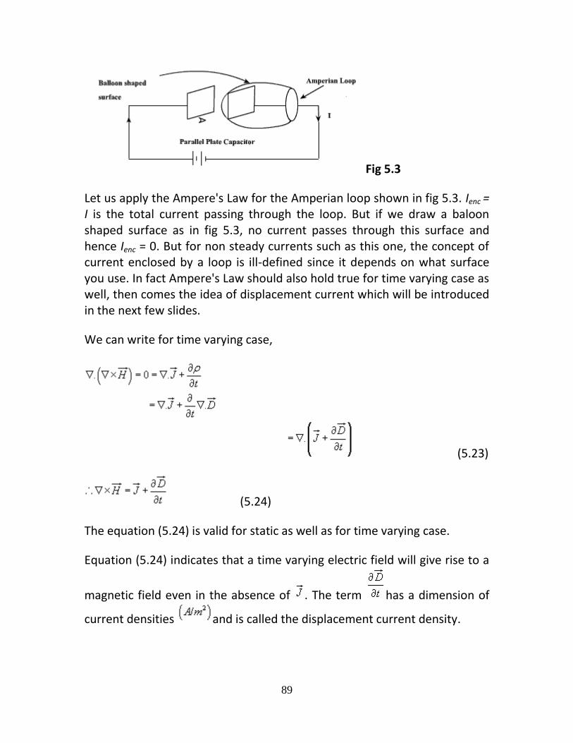
89

Fig 5.3

Let us apply the Ampere's Law for the Amperian loop shown in fig 5.3. Ienc = I is the total current passing through the loop. But if we draw a baloon shaped surface as in fig 5.3, no current passes through this surface and hence Ienc = 0. But for non steady currents such as this one, the concept of current enclosed by a loop is ill-defined since it depends on what surface you use. In fact Ampere's Law should also hold true for time varying case as well, then comes the idea of displacement current which will be introduced in the next few slides.

We can write for time varying case,

(5.23)

(5.24)

The equation (5.24) is valid for static as well as for time varying case.

Equation (5.24) indicates that a time varying electric field will give rise to a

magnetic field even in the absence of . The term has a dimension of

current densities and is called the displacement current density.

90

Introduction of in equation is one of the major contributions of Jame's Clerk Maxwell. The modified set of equations

(5.25a)

(5.25b)

(5.25c)

(5.25d)

is known as the Maxwell's equation and this set of equations apply in the

time varying scenario, static fields are being a particular case .

In the integral form

(5.26a)

(5.26b)

(5.26c)

(5.26d)

The modification of Ampere's law by Maxwell has led to the development of a unified electromagnetic field theory. By introducing the displacement current term, Maxwell could predict the propagation of EM waves. Existence of EM waves was later demonstrated by Hertz experimentally which led to the new era of radio communication.

Boundary Conditions for Electromagnetic fields

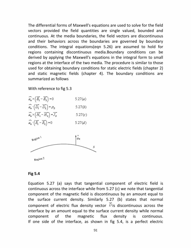
91

The differential forms of Maxwell's equations are used to solve for the field vectors provided the field quantities are single valued, bounded and continuous. At the media boundaries, the field vectors are discontinuous and their behaviors across the boundaries are governed by boundary conditions. The integral equations(eqn 5.26) are assumed to hold for regions containing discontinuous media.Boundary conditions can be derived by applying the Maxwell's equations in the integral form to small regions at the interface of the two media. The procedure is similar to those used for obtaining boundary conditions for static electric fields (chapter 2) and static magnetic fields (chapter 4). The boundary conditions are summarized as follows

With reference to fig 5.3

Fig 5.4

Equation 5.27 (a) says that tangential component of electric field is continuous across the interface while from 5.27 (c) we note that tangential component of the magnetic field is discontinuous by an amount equal to the surface current density. Similarly 5.27 (b) states that normal

component of electric flux density vector is discontinuous across the interface by an amount equal to the surface current density while normal component of the magnetic flux density is continuous. If one side of the interface, as shown in fig 5.4, is a perfect electric

92

conductor, say region 2, a surface current can exist even though is zero as . Thus eqn 5.27(a) and (c) reduces to

Wave equation and their solution:

From equation 5.25 we can write the Maxwell's equations in the differential form as

Let us consider a source free uniform medium having dielectric constant , magnetic permeability and conductivity . The above set of equations can be written as

Using the vector identity ,

We can write from 5.29(b)

93

or

Substituting from 5.29(a)

But in source free medium (eqn 5.29(c))

(5.30)

In the same manner for equation eqn 5.29(a)

Since from eqn 5.29(d), we can write

(5.31)

These two equations

94

are known as wave equations.

It may be noted that the field components are functions of both space and

time. For example, if we consider a Cartesian co ordinate system,

essentially represents and . For simplicity, we consider

propagation in free space , i.e. , and . The wave eqn in equations 5.30 and 5.31 reduces to

Further simplifications can be made if we consider in Cartesian co ordinate

system a special case where are considered to be independent in

two dimensions, say are assumed to be independent of y and z. Such waves are called plane waves.

From eqn (5.32 (a)) we can write

The vector wave equation is equivalent to the three scalar equations

95

Since we have ,

As we have assumed that the field components are independent of y and z eqn (5.34) reduces to

(5.35)

i.e. there is no variation of Ex in the x direction.

Further, from 5.33(a), we find that implies which requires any three of the conditions to be satisfied: (i) Ex=0, (ii)Ex = constant, (iii)Ex increasing uniformly with time.

A field component satisfying either of the last two conditions (i.e (ii) and (iii))is not a part of a plane wave motion and hence Ex is taken to be equal to zero. Therefore, a uniform plane wave propagating in x direction does not have a field component (E or H) acting along x.

Without loss of generality let us now consider a plane wave having Ey component only (Identical results can be obtained for Ez component) .

The equation involving such wave propagation is given by

The above equation has a solution of the form

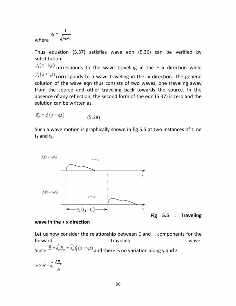
96

where

Thus equation (5.37) satisfies wave eqn (5.36) can be verified by substitution.

corresponds to the wave traveling in the + x direction while

corresponds to a wave traveling in the -x direction. The general solution of the wave eqn thus consists of two waves, one traveling away from the source and other traveling back towards the source. In the absence of any reflection, the second form of the eqn (5.37) is zero and the solution can be written as

(5.38)

Such a wave motion is graphically shown in fig 5.5 at two instances of time t1 and t2.

Fig 5.5 : Traveling wave in the + x direction

Let us now consider the relationship between E and H components for the forward traveling wave.

Since and there is no variation along y and z.

97

Since only z component of exists, from (5.29(b))

(5.39)

and from (5.29(a)) with , only Hz component of magnetic field being present

(5.40)

Substituting Ey from (5.38)

The constant of integration means that a field independent of x may also exist. However, this field will not be a part of the wave motion.

Hence (5.41)

which relates the E and H components of the traveling wave.

98

is called the characteristic or intrinsic impedance of the free space

ASSIGNMENT PROBLEMS

1. A rectangular loop of area rotates at rad/s in a magnetic fields of B Wb/m2 normal to the axis of rotation. If the loop has N turns determine the induced voltage in the loop.

2. If the electric field component in a nonmagnetic dielectric medium is given by

determine the dielectric constant and the corresponding .

3. A vector field in phasor form is given by

Express in instantaneous form.

99

Unit V Electromagnetic waves

In the previous chapter we introduced the equations pertaining to wave propagation and discussed how the wave equations are modified for time harmonic case. In this chapter we discuss in detail a particular form of electromagnetic wave propagation called 'plane waves'. The Helmhotz Equation: In source free linear isotropic medium, Maxwell equations in phasor form are,

or,

or,

or, where

An identical equation can be derived for .

i.e.,

These equations

are called homogeneous vector Helmholtz's equation.

100

is called the wave number or propagation constant of the medium.

Plane waves in Lossless medium:

In a lossless medium, are real numbers, so k is real.

In Cartesian coordinates each of the equations 6.1(a) and 6.1(b) are equivalent to three scalar Helmholtz's equations, one each in the components Ex, Ey and Ez or Hx , Hy, Hz.

For example if we consider Ex component we can write

.................................................(6.2)

A uniform plane wave is a particular solution of Maxwell's equation assuming electric field (and magnetic field) has same magnitude and phase in infinite planes perpendicular to the direction of propagation. It may be noted that in the strict sense a uniform plane wave doesn't exist in practice as creation of such waves are possible with sources of infinite extent. However, at large distances from the source, the wavefront or the surface of the constant phase becomes almost spherical and a small portion of this large sphere can be considered to plane. The characteristics of plane waves are simple and useful for studying many practical scenarios.

Let us consider a plane wave which has only Ex component and propagating along z . Since the plane wave will have no variation along the plane

perpendicular to z i.e., xy plane, . The Helmholtz's equation (6.2) reduces to,

.........................................................................(6.3)

The solution to this equation can be written as

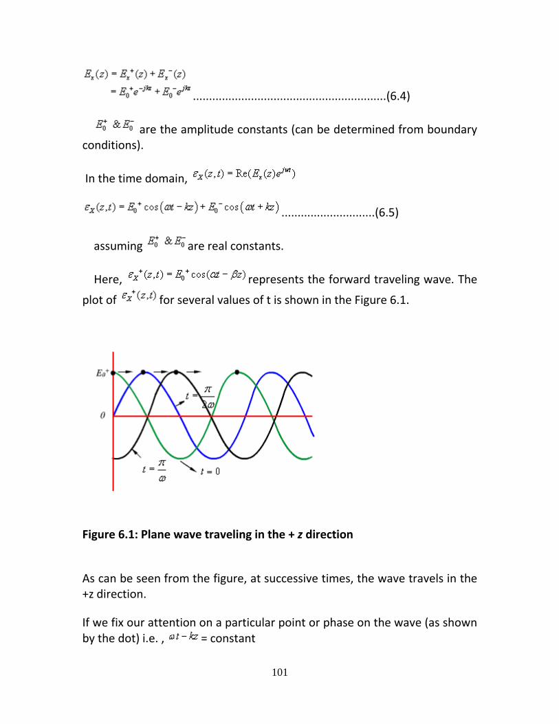
101

............................................................(6.4)

are the amplitude constants (can be determined from boundary conditions).

In the time domain,

.............................(6.5)

assuming are real constants.

Here, represents the forward traveling wave. The

plot of for several values of t is shown in the Figure 6.1.

Figure 6.1: Plane wave traveling in the + z direction

As can be seen from the figure, at successive times, the wave travels in the +z direction.

If we fix our attention on a particular point or phase on the wave (as shown by the dot) i.e. , = constant

102

Then we see that as t is increased to , z also should increase to so that

Or,

Or,

When ,

we write = phase velocity .

.....................................(6.6)

If the medium in which the wave is propagating is free space i.e.,

Then

Where 'C' is the speed of light. That is plane EM wave travels in free space with the speed of light.

The wavelength is defined as the distance between two successive maxima (or minima or any other reference points).

i.e.,

or,

or,

Substituting ,

103

or, ................................(6.7)

Thus wavelength also represents the distance covered in one oscillation

of the wave. Similarly, represents a plane wave traveling in the -z direction.

The associated magnetic field can be found as follows:

From (6.4),

=

= ............(6.8)

where is the intrinsic impedance of the medium. When the wave travels in free space

is the intrinsic impedance of the free space.

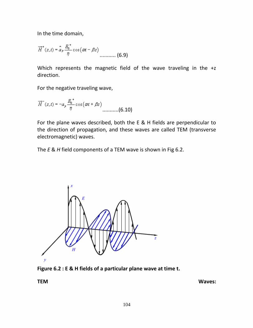
104

In the time domain,

........... (6.9)

Which represents the magnetic field of the wave traveling in the +z direction.

For the negative traveling wave,

...........(6.10)

For the plane waves described, both the E & H fields are perpendicular to the direction of propagation, and these waves are called TEM (transverse electromagnetic) waves.

The E & H field components of a TEM wave is shown in Fig 6.2.

Figure 6.2 : E & H fields of a particular plane wave at time t.

TEM Waves:

105

So far we have considered a plane electromagnetic wave propagating in the z-direction. Let us now consider the propagation of a uniform plane wave in any arbitrary direction that doesn't necessarily coincides with an axis.

For a uniform plane wave propagating in z-direction

is a constant vector........................... (6.11)

The more general form of the above equation is

........................................... (6.12)

This equation satisfies Helmholtz's equation provided,

........................... (6.13)

We define wave number vector ........................... (6.14)

And radius vector from the origin

........................... (6.15)

Therefore we can write

........................... (6.16)

Here =constant is a plane of constant phase and uniform amplitude just

in the case of ,

z =constant denotes a plane of constant phase and uniform amplitude.

If the region under consideration is charge free,

106

Using the vector identity and noting that is constant we can write,

......................(6.17)

i.e., is transverse to the direction of the propagation.

The corresponding magnetic field can be computed as follows:

Using the vector identity,

Since is constant we can write,

107

.....................(6.18)

Where is the intrinsic impedance of the medium. We observe that is

perpendicular to both and . Thus the electromagnetic wave

represented by and is a TEM wave.

Plane waves in a lossy medium :

In a lossy medium, the EM wave looses power as it propagates. Such a medium is conducting with conductivity and we can write:

.....................(6.19)

Where is called the complex permittivity.

We have already discussed how an external electric field can polarize a dielectric and give rise to bound charges. When the external electric field is time varying, the polarization vector will vary with the same frequency as that of the applied field. As the frequency of the applied filed increases, the inertia of the charge particles tend to prevent the particle displacement keeping pace with the applied field changes. This results in frictional damping mechanism causing power loss.

In addition, if the material has an appreciable amount of free charges, there will be ohmic losses. It is customary to include the effect of damping and

ohmic losses in the imaginary part of . An equivalent conductivity represents all losses.

The ratio is called loss tangent as this quantity is a measure of the power loss.

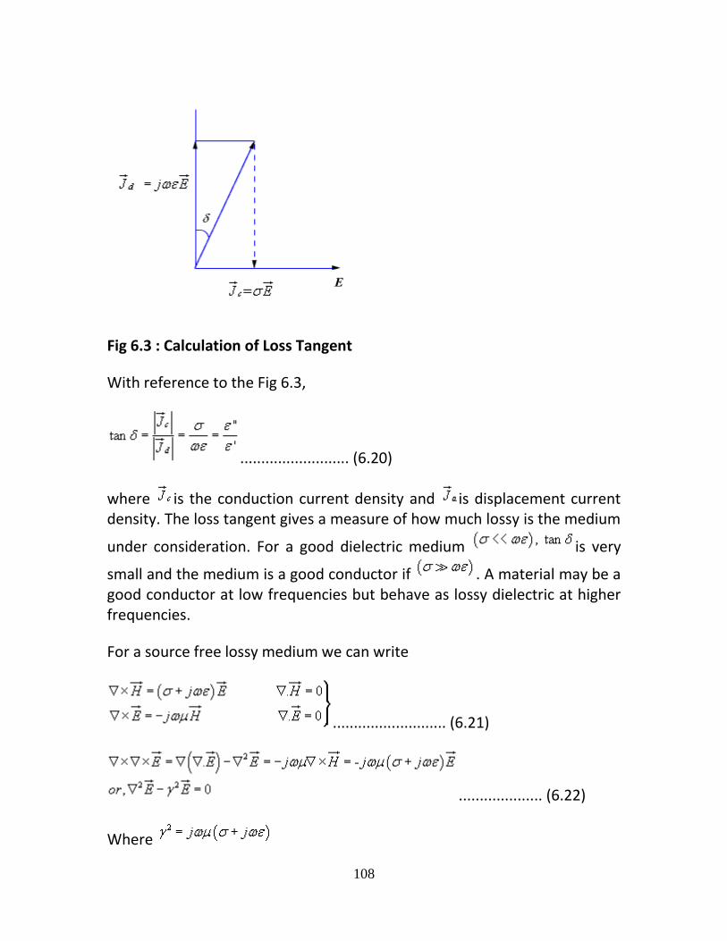
108

Fig 6.3 : Calculation of Loss Tangent

With reference to the Fig 6.3,

.......................... (6.20)

where is the conduction current density and is displacement current density. The loss tangent gives a measure of how much lossy is the medium

under consideration. For a good dielectric medium is very

small and the medium is a good conductor if . A material may be a good conductor at low frequencies but behave as lossy dielectric at higher frequencies.

For a source free lossy medium we can write

........................... (6.21)

.................... (6.22)

Where

109

Proceeding in the same manner we can write,

is called the propagation constant.

The real and imaginary parts and of the propagation constant can be computed as follows:

And

................... (6.23a)

Similarly ................... (6.23b)

Let us now consider a plane wave that has only x -component of electric field and propagate along z .

110

................................... (6.24)

Considering only the forward traveling wave

................................... (6.25)

Similarly, from , we can find

..................................... (6.26)

Where

..................................... (6.27)

From (6.25) and (6.26) we find that as the wave propagates along z, it

decreases in amplitude by a factor . Therefore is known as

attenuation constant. Further and are out of phase by an angle .

For low loss dielectric, , i.e., .

Using the above condition approximate expression for and can be obtained as follows:

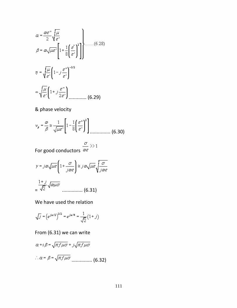
111

............. (6.29)

& phase velocity

............... (6.30)

For good conductors

= ............... (6.31)

We have used the relation

From (6.31) we can write

............... (6.32)

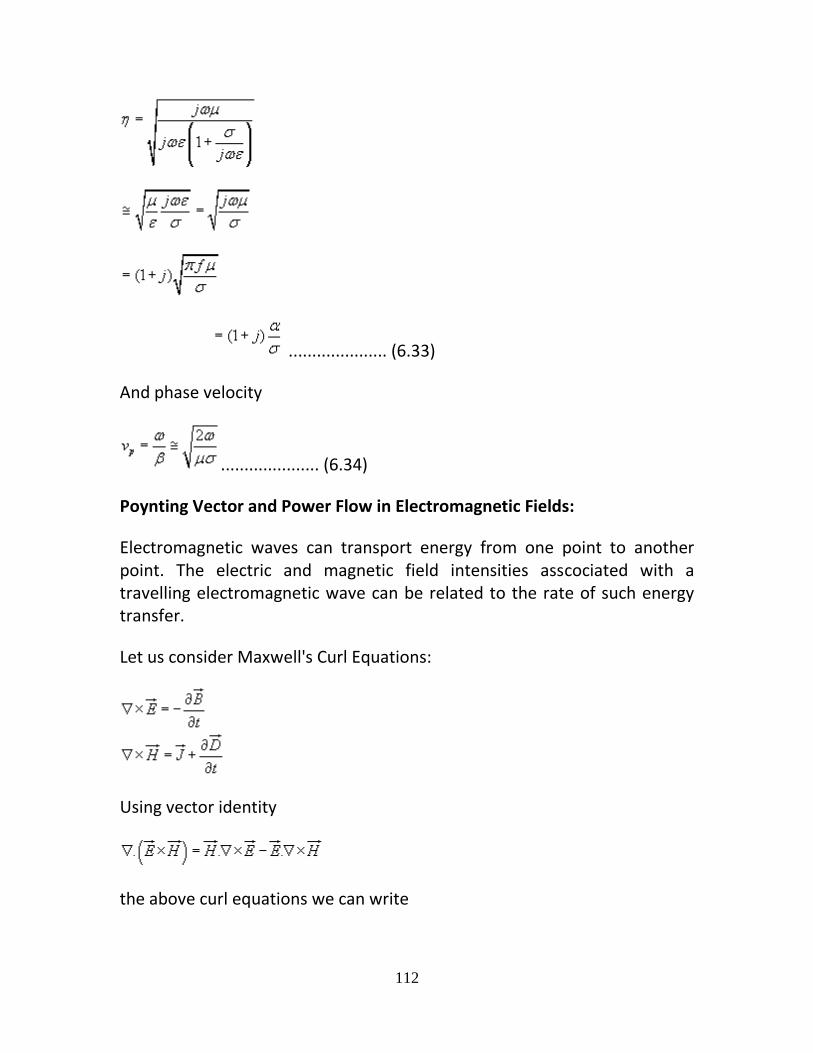
112

..................... (6.33)

And phase velocity

..................... (6.34)

Poynting Vector and Power Flow in Electromagnetic Fields:

Electromagnetic waves can transport energy from one point to another point. The electric and magnetic field intensities asscociated with a travelling electromagnetic wave can be related to the rate of such energy transfer.

Let us consider Maxwell's Curl Equations:

Using vector identity

the above curl equations we can write

113

.............................................(6.35)

In simple medium where and are constant, we can write

and

Applying Divergence theorem we can write,

...........................(6.36)

The term represents the rate of change of energy

stored in the electric and magnetic fields and the term represents the power dissipation within the volume. Hence right hand side of the equation (6.36) represents the total decrease in power within the volume under consideration.

The left hand side of equation (6.36) can be written as

where (W/mt2) is called the Poynting vector and it represents the power density vector associated with the electromagnetic field. The integration of the Poynting vector over any closed surface gives the net power flowing out of the surface. Equation (6.36) is referred to as Poynting theorem and it states that the net power flowing out of a given volume is

114

equal to the time rate of decrease in the energy stored within the volume minus the conduction losses.

Poynting vector for the time harmonic case:

For time harmonic case, the time variation is of the form , and we have seen that instantaneous value of a quantity is the real part of the product

of a phasor quantity and when is used as reference. For example, if we consider the phasor

then we can write the instanteneous field as

.................................(6.37)

when E0 is real. Let us consider two instanteneous quantities A and B such that

where A and B are the phasor quantities.

i.e,

Therefore,

..............................(6.39)

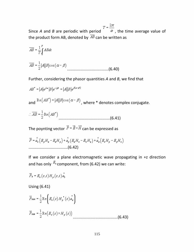
115

Since A and B are periodic with period , the time average value of

the product form AB, denoted by can be written as

.....................................(6.40)

Further, considering the phasor quantities A and B, we find that

and , where * denotes complex conjugate.

..............................................(6.41)

The poynting vector can be expressed as

...................................(6.42)

If we consider a plane electromagnetic wave propagating in +z direction

and has only component, from (6.42) we can write:

Using (6.41)

........................................(6.43)

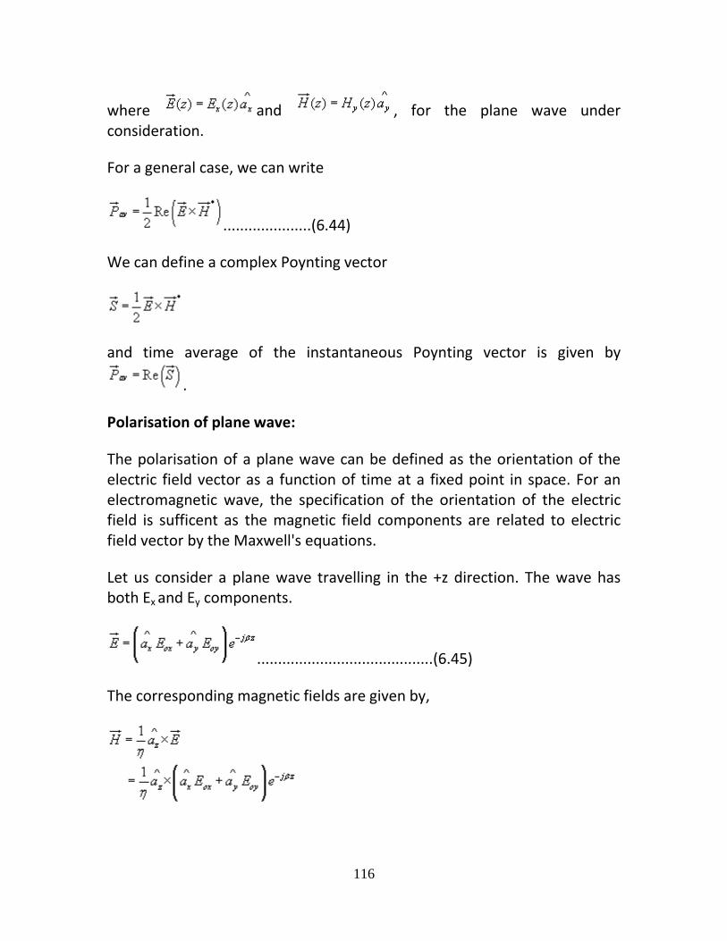
116

where and , for the plane wave under consideration.

For a general case, we can write

.....................(6.44)

We can define a complex Poynting vector

and time average of the instantaneous Poynting vector is given by

.

Polarisation of plane wave:

The polarisation of a plane wave can be defined as the orientation of the electric field vector as a function of time at a fixed point in space. For an electromagnetic wave, the specification of the orientation of the electric field is sufficent as the magnetic field components are related to electric field vector by the Maxwell's equations.

Let us consider a plane wave travelling in the +z direction. The wave has both Ex and Ey components.

..........................................(6.45)

The corresponding magnetic fields are given by,

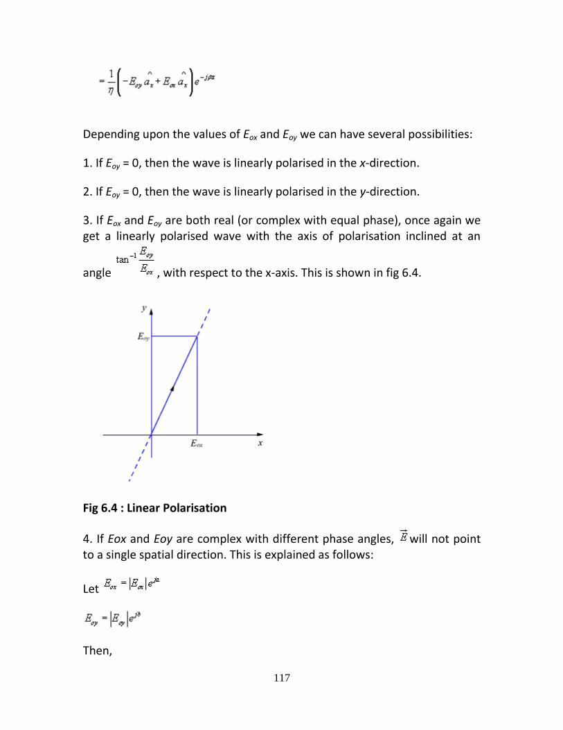
117

Depending upon the values of Eox and Eoy we can have several possibilities:

1. If Eoy = 0, then the wave is linearly polarised in the x-direction.

2. If Eoy = 0, then the wave is linearly polarised in the y-direction.

3. If Eox and Eoy are both real (or complex with equal phase), once again we get a linearly polarised wave with the axis of polarisation inclined at an

angle , with respect to the x-axis. This is shown in fig 6.4.

Fig 6.4 : Linear Polarisation

4. If Eox and Eoy are complex with different phase angles, will not point to a single spatial direction. This is explained as follows:

Let

Then,

118

and ....................................(6.46)

To keep the things simple, let us consider a =0 and . Further, let us study the nature of the electric field on the z =0 plain.

From equation (6.46) we find that,

.....................................(6.47)

and the electric field vector at z = 0 can be written as

.............................................(6.48)

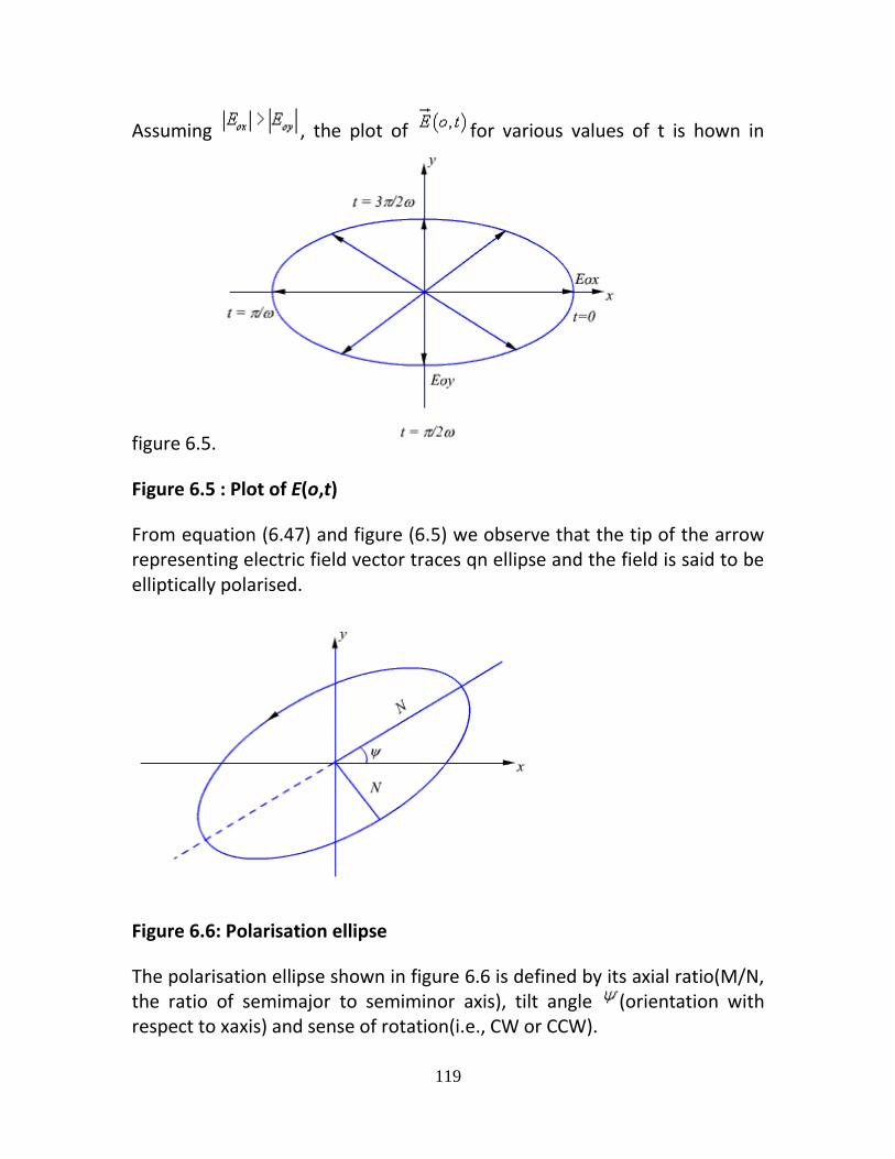
119

Assuming , the plot of for various values of t is hown in

figure 6.5.

Figure 6.5 : Plot of E(o,t)

From equation (6.47) and figure (6.5) we observe that the tip of the arrow representing electric field vector traces qn ellipse and the field is said to be elliptically polarised.

Figure 6.6: Polarisation ellipse

The polarisation ellipse shown in figure 6.6 is defined by its axial ratio(M/N, the ratio of semimajor to semiminor axis), tilt angle (orientation with respect to xaxis) and sense of rotation(i.e., CW or CCW).

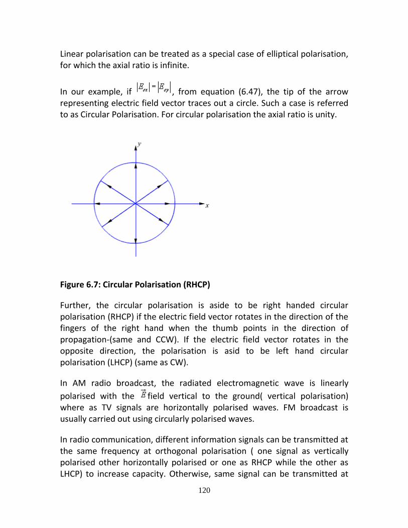
120

Linear polarisation can be treated as a special case of elliptical polarisation, for which the axial ratio is infinite.

In our example, if , from equation (6.47), the tip of the arrow representing electric field vector traces out a circle. Such a case is referred to as Circular Polarisation. For circular polarisation the axial ratio is unity.

Figure 6.7: Circular Polarisation (RHCP)

Further, the circular polarisation is aside to be right handed circular polarisation (RHCP) if the electric field vector rotates in the direction of the fingers of the right hand when the thumb points in the direction of propagation-(same and CCW). If the electric field vector rotates in the opposite direction, the polarisation is asid to be left hand circular polarisation (LHCP) (same as CW).

In AM radio broadcast, the radiated electromagnetic wave is linearly

polarised with the field vertical to the ground( vertical polarisation) where as TV signals are horizontally polarised waves. FM broadcast is usually carried out using circularly polarised waves.

In radio communication, different information signals can be transmitted at the same frequency at orthogonal polarisation ( one signal as vertically polarised other horizontally polarised or one as RHCP while the other as LHCP) to increase capacity. Otherwise, same signal can be transmitted at

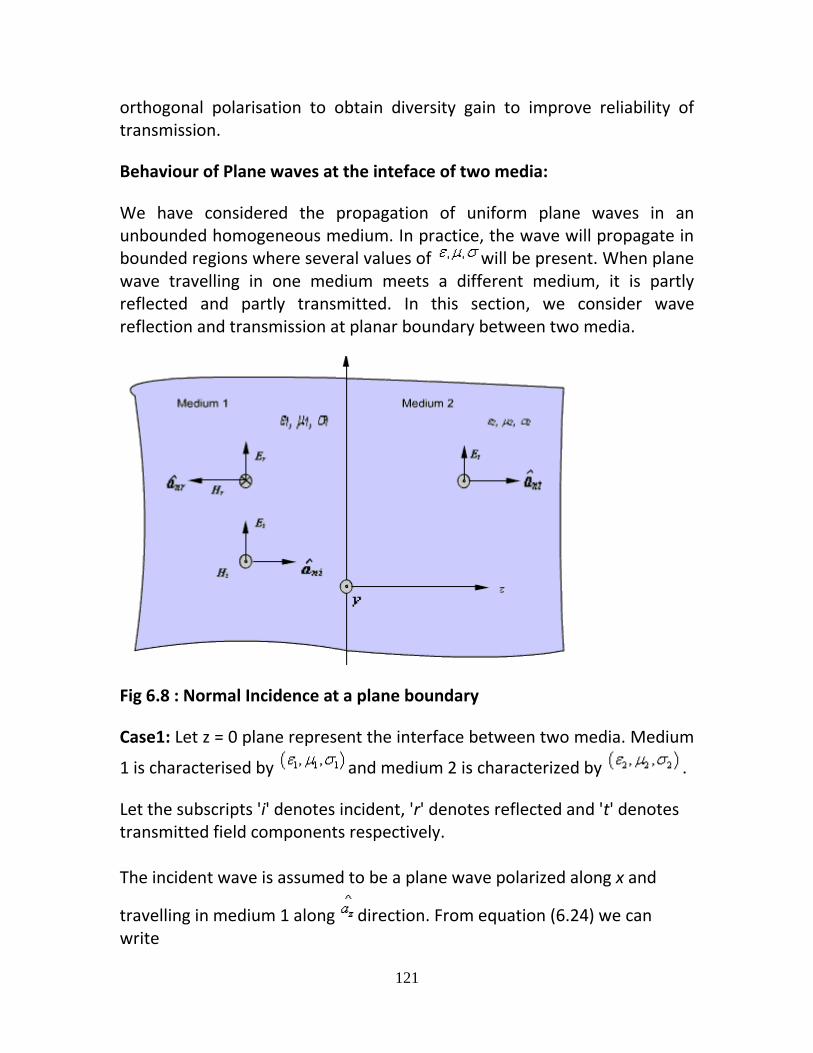
121

orthogonal polarisation to obtain diversity gain to improve reliability of transmission.

Behaviour of Plane waves at the inteface of two media:

We have considered the propagation of uniform plane waves in an unbounded homogeneous medium. In practice, the wave will propagate in bounded regions where several values of will be present. When plane wave travelling in one medium meets a different medium, it is partly reflected and partly transmitted. In this section, we consider wave reflection and transmission at planar boundary between two media.

Fig 6.8 : Normal Incidence at a plane boundary

Case1: Let z = 0 plane represent the interface between two media. Medium

1 is characterised by and medium 2 is characterized by .

Let the subscripts 'i' denotes incident, 'r' denotes reflected and 't' denotes transmitted field components respectively. The incident wave is assumed to be a plane wave polarized along x and

travelling in medium 1 along direction. From equation (6.24) we can write

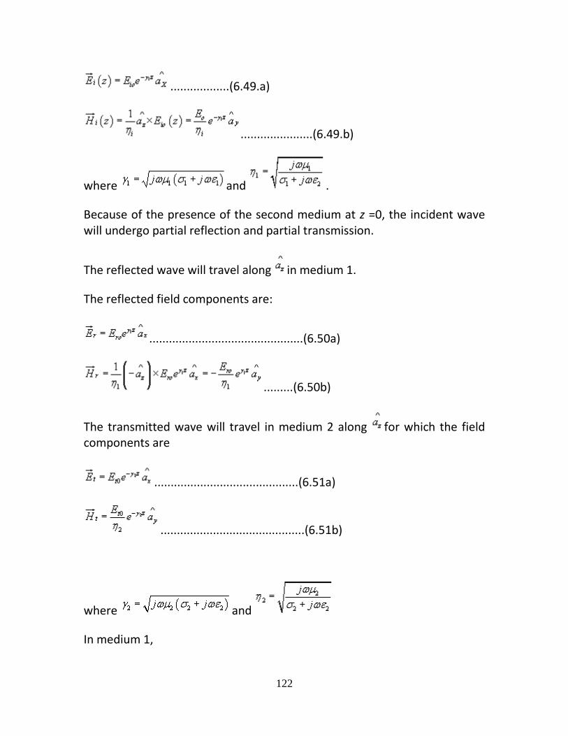
122

..................(6.49.a)

......................(6.49.b)

where and .

Because of the presence of the second medium at z =0, the incident wave will undergo partial reflection and partial transmission.

The reflected wave will travel along in medium 1.

The reflected field components are:

...............................................(6.50a)

.........(6.50b)

The transmitted wave will travel in medium 2 along for which the field components are

............................................(6.51a)

............................................(6.51b)

where and

In medium 1,

123

and

and in medium 2,

and

Applying boundary conditions at the interface z = 0, i.e., continuity of tangential field components and noting that incident, reflected and transmitted field components are tangential at the boundary, we can write

&

From equation 6.49 to 6.51 we get,

................................................................(6.52a)

..............................................................(6.52b)

Eliminating Eto ,

or,

or,

...............(6.53)

is called the reflection coefficient.

From equation (6.52), we can write

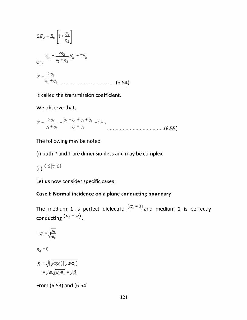
124

or,

........................................(6.54)

is called the transmission coefficient.

We observe that,

........................................(6.55)

The following may be noted

(i) both and T are dimensionless and may be complex

(ii)

Let us now consider specific cases:

Case I: Normal incidence on a plane conducting boundary

The medium 1 is perfect dielectric and medium 2 is perfectly

conducting .

From (6.53) and (6.54)

125

= -1

and T =0

Hence the wave is not transmitted to medium 2, it gets reflected entirely from the interface to the medium 1.

& .................................(6.56)

Proceeding in the same manner for the magnetic field in region 1, we can show that,

...................................................................................(6.57)

The wave in medium 1 thus becomes a standing wave due to the super position of a forward travelling wave and a backward travelling wave. For a

given ' t', both and vary sinusoidally with distance measured from z = 0. This is shown in figure 6.9.

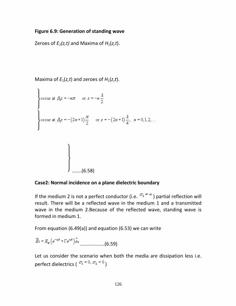
126

Figure 6.9: Generation of standing wave

Zeroes of E1(z,t) and Maxima of H1(z,t).

Maxima of E1(z,t) and zeroes of H1(z,t).

.......(6.58)

Case2: Normal incidence on a plane dielectric boundary

If the medium 2 is not a perfect conductor (i.e. ) partial reflection will result. There will be a reflected wave in the medium 1 and a transmitted wave in the medium 2.Because of the reflected wave, standing wave is formed in medium 1.

From equation (6.49(a)) and equation (6.53) we can write

..................(6.59)

Let us consider the scenario when both the media are dissipation less i.e.

perfect dielectrics ( )

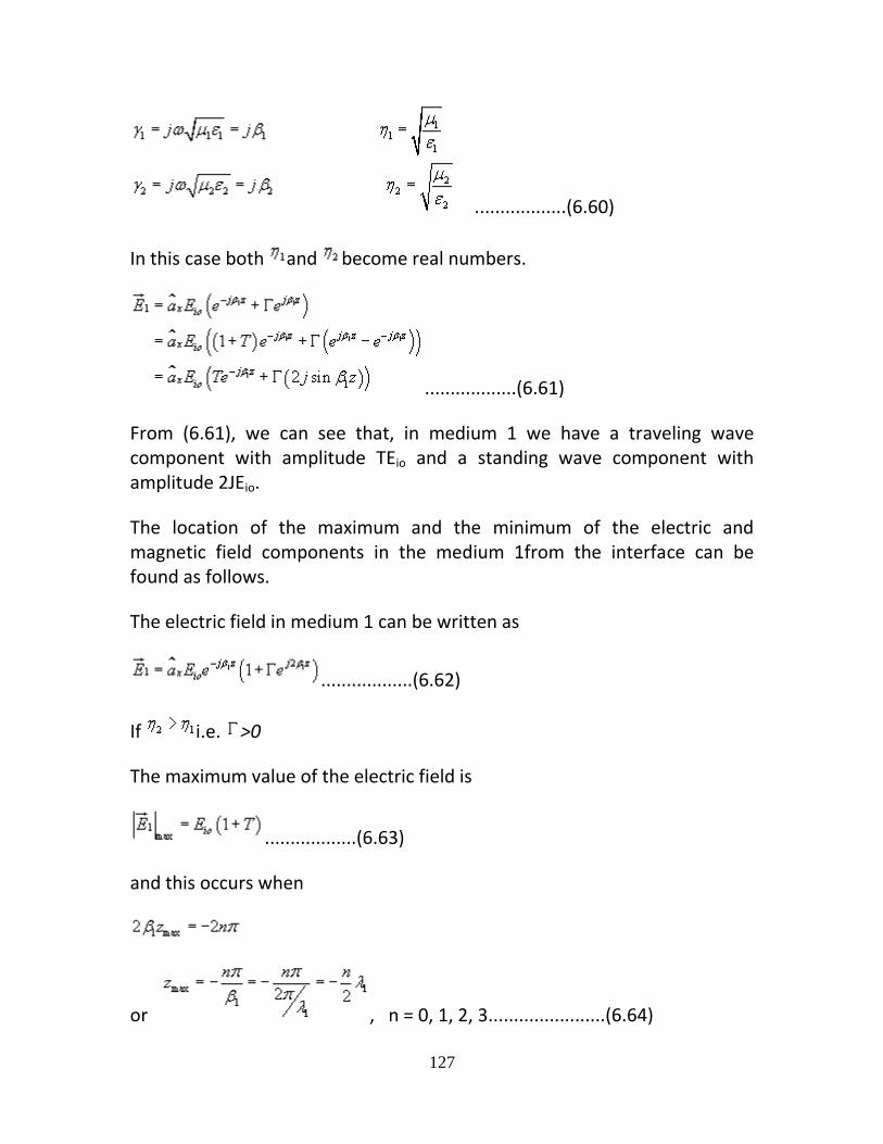
127

..................(6.60)

In this case both and become real numbers.

..................(6.61)

From (6.61), we can see that, in medium 1 we have a traveling wave component with amplitude TEio and a standing wave component with amplitude 2JEio.

The location of the maximum and the minimum of the electric and magnetic field components in the medium 1from the interface can be found as follows.

The electric field in medium 1 can be written as

..................(6.62)

If i.e. >0

The maximum value of the electric field is

..................(6.63)

and this occurs when

or , n = 0, 1, 2, 3.......................(6.64)

128

The minimum value of is

.................(6.65)

And this occurs when

or , n = 0, 1, 2, 3.............................(6.66)

For i.e. <0

The maximum value of is which occurs at the zmin locations and

the minimum value of is which occurs at zmax locations as given by the equations (6.64) and (6.66).

From our discussions so far we observe that can be written as

.................(6.67)

The quantity S is called as the standing wave ratio.

As the range of S is given by

From (6.62), we can write the expression for the magnetic field in medium 1 as

.................(6.68)

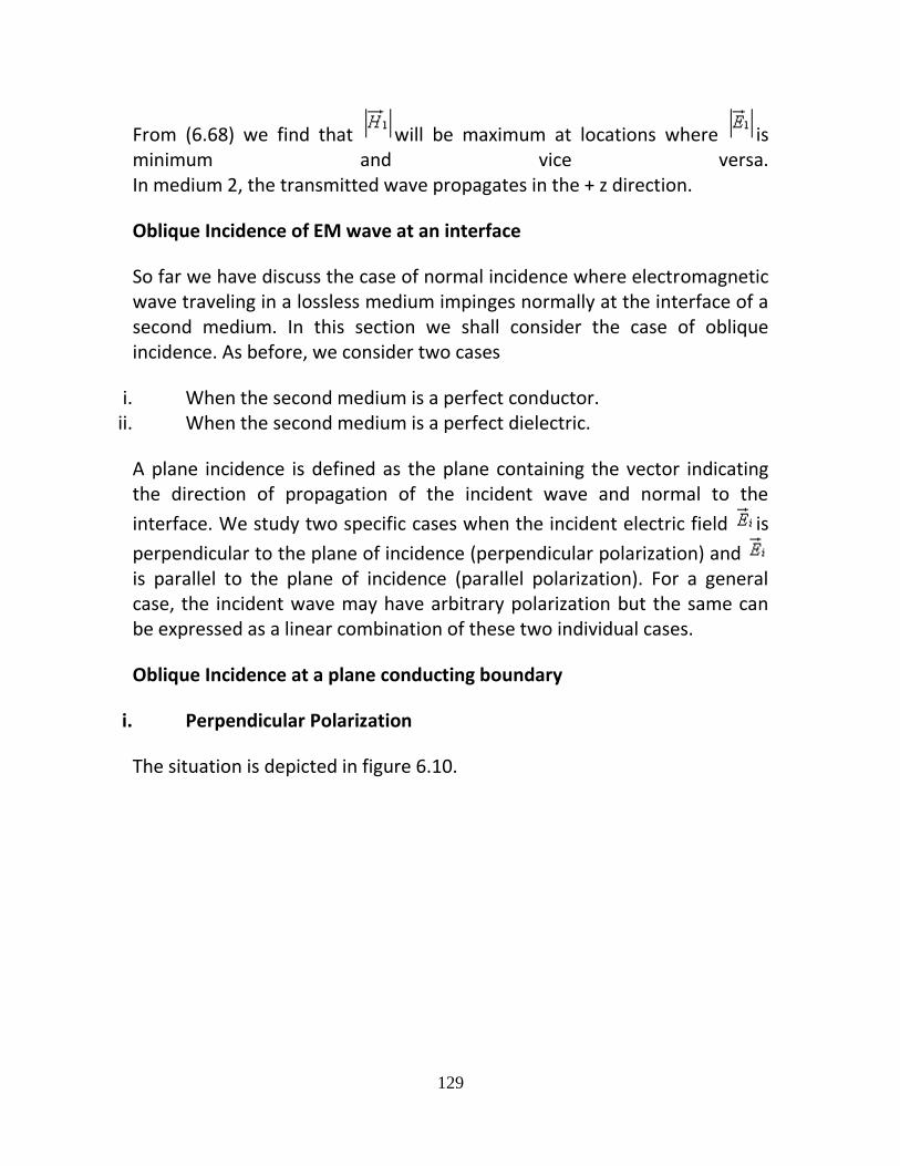
129

From (6.68) we find that will be maximum at locations where is minimum and vice versa. In medium 2, the transmitted wave propagates in the + z direction.

Oblique Incidence of EM wave at an interface

So far we have discuss the case of normal incidence where electromagnetic wave traveling in a lossless medium impinges normally at the interface of a second medium. In this section we shall consider the case of oblique incidence. As before, we consider two cases

i. When the second medium is a perfect conductor. ii. When the second medium is a perfect dielectric.

A plane incidence is defined as the plane containing the vector indicating the direction of propagation of the incident wave and normal to the

interface. We study two specific cases when the incident electric field is

perpendicular to the plane of incidence (perpendicular polarization) and is parallel to the plane of incidence (parallel polarization). For a general case, the incident wave may have arbitrary polarization but the same can be expressed as a linear combination of these two individual cases.

Oblique Incidence at a plane conducting boundary

i. Perpendicular Polarization

The situation is depicted in figure 6.10.

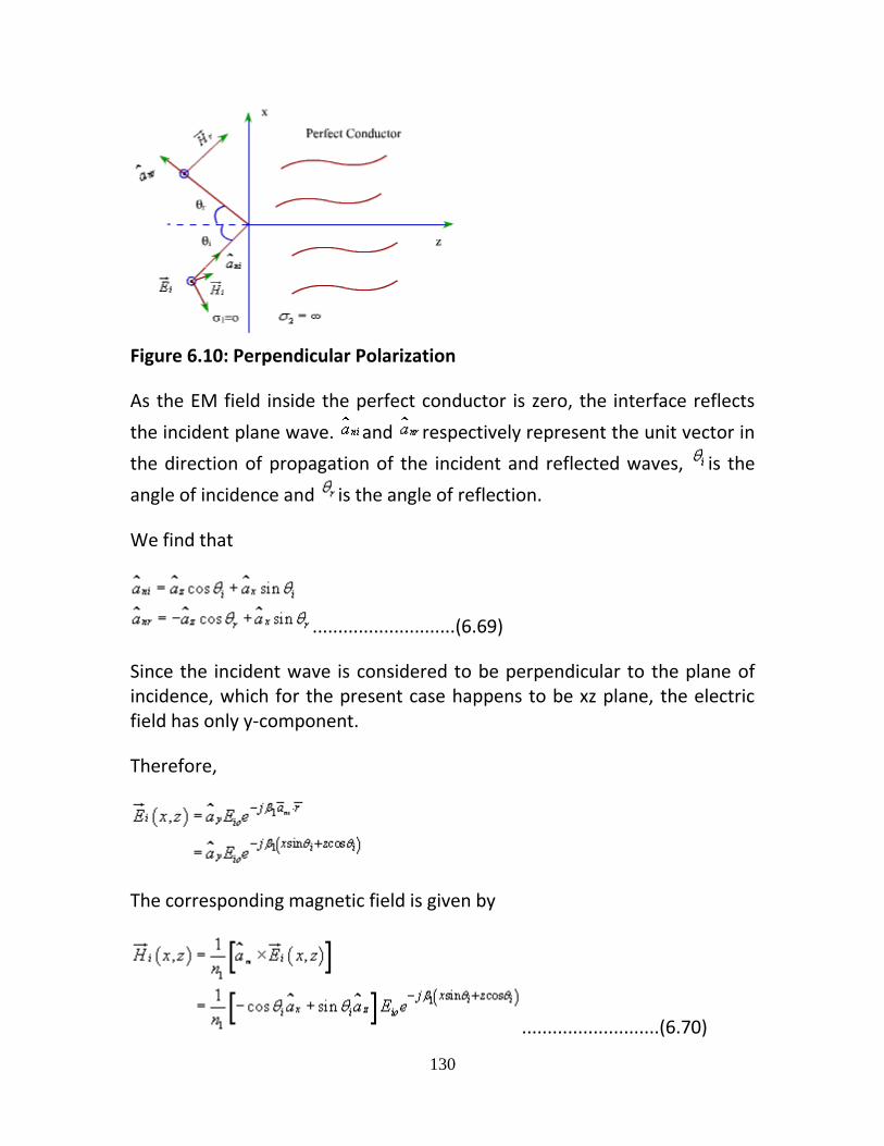
130

Figure 6.10: Perpendicular Polarization

As the EM field inside the perfect conductor is zero, the interface reflects

the incident plane wave. and respectively represent the unit vector in

the direction of propagation of the incident and reflected waves, is the

angle of incidence and is the angle of reflection.

We find that

............................(6.69)

Since the incident wave is considered to be perpendicular to the plane of incidence, which for the present case happens to be xz plane, the electric field has only y-component.

Therefore,

The corresponding magnetic field is given by

...........................(6.70)

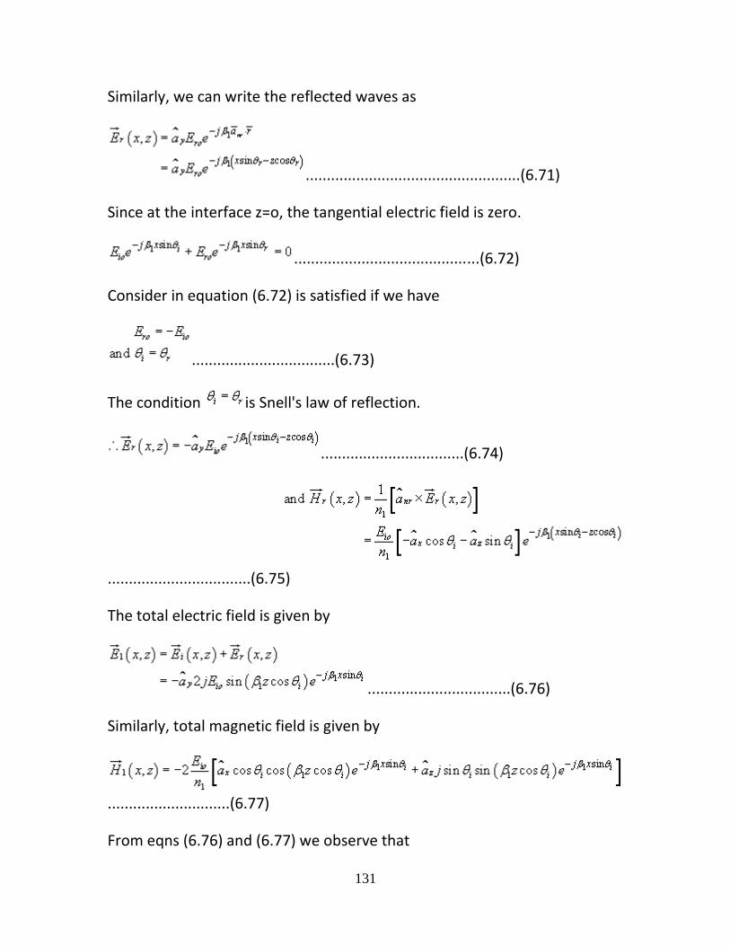
131

Similarly, we can write the reflected waves as

...................................................(6.71)

Since at the interface z=o, the tangential electric field is zero.

............................................(6.72)

Consider in equation (6.72) is satisfied if we have

..................................(6.73)

The condition is Snell's law of reflection.

..................................(6.74)

..................................(6.75)

The total electric field is given by

..................................(6.76)

Similarly, total magnetic field is given by

.............................(6.77)

From eqns (6.76) and (6.77) we observe that

132

1. Along z direction i.e. normal to the boundary

y component of and x component of maintain standing wave

patterns according to and where . No

average power propagates along z as y component of and x

component of are out of phase. 2. Along x i.e. parallel to the interface

y component of and z component of are in phase (both time and space) and propagate with phase velocity

.............................(6.78)

The wave propagating along the x direction has its amplitude varying with z and hence constitutes a non uniform plane wave. Further, only electric

field is perpendicular to the direction of propagation (i.e. x), the magnetic field has component along the direction of propagation. Such waves are called transverse electric or TE waves.

ii. Parallel Polarization:

In this case also and are given by equations (6.69). Here and have only y component.

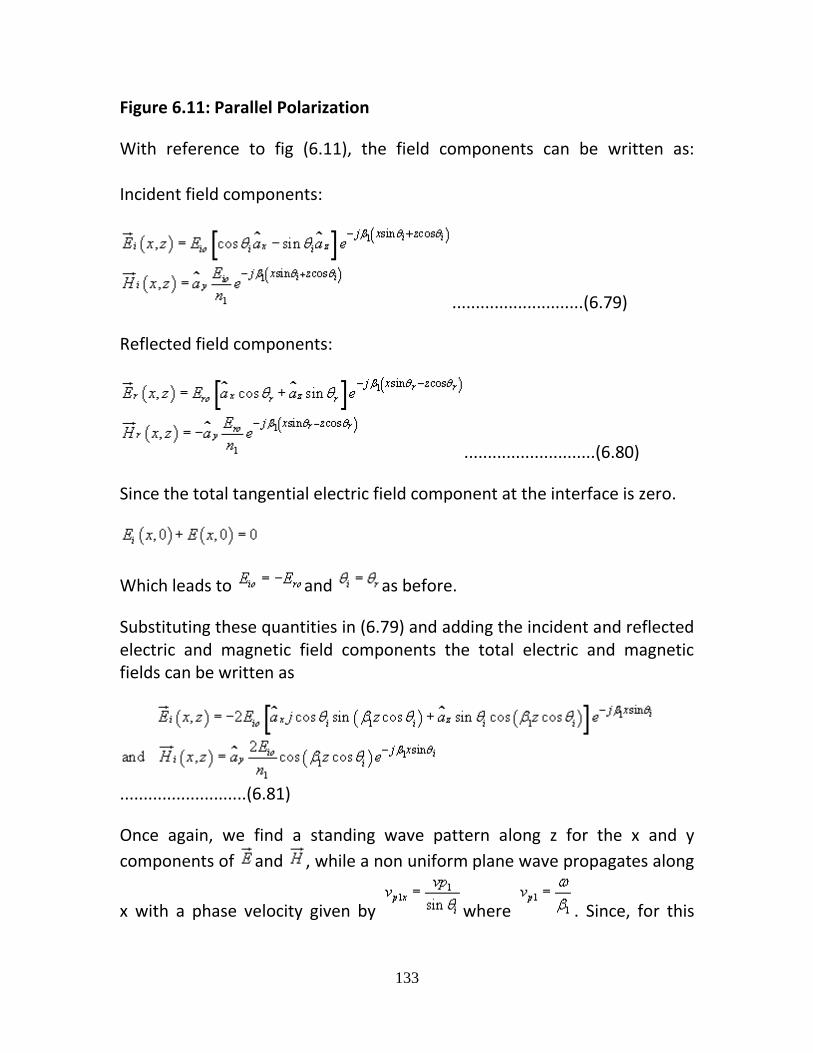
133

Figure 6.11: Parallel Polarization

With reference to fig (6.11), the field components can be written as: Incident field components:

............................(6.79)

Reflected field components:

............................(6.80)

Since the total tangential electric field component at the interface is zero.

Which leads to and as before.

Substituting these quantities in (6.79) and adding the incident and reflected electric and magnetic field components the total electric and magnetic fields can be written as

...........................(6.81)

Once again, we find a standing wave pattern along z for the x and y

components of and , while a non uniform plane wave propagates along

x with a phase velocity given by where . Since, for this

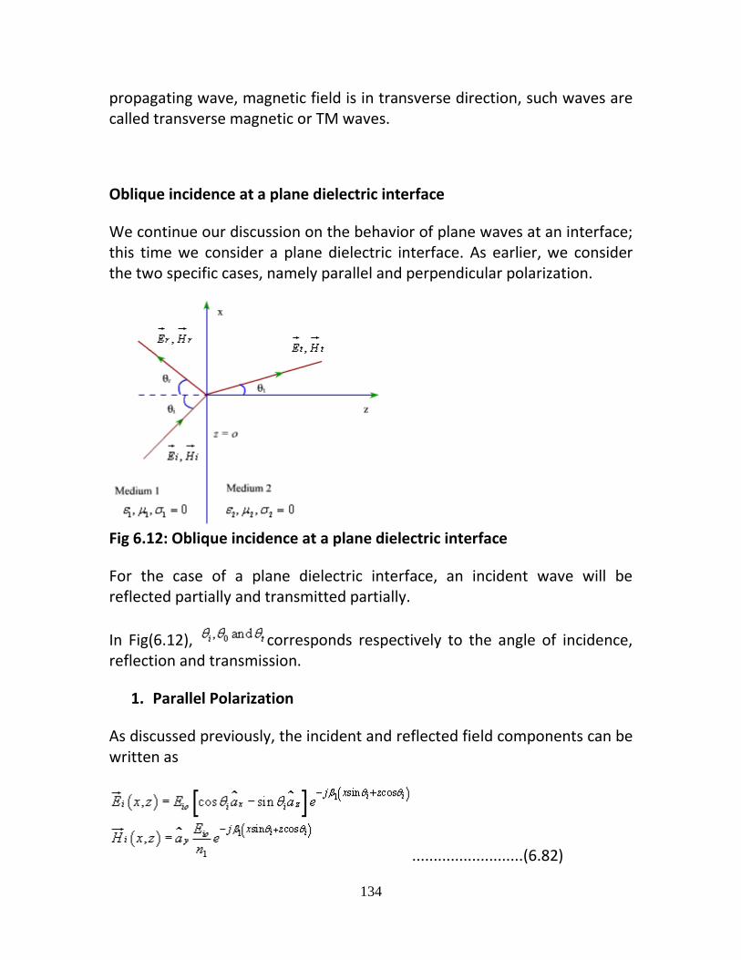
134

propagating wave, magnetic field is in transverse direction, such waves are called transverse magnetic or TM waves.

Oblique incidence at a plane dielectric interface

We continue our discussion on the behavior of plane waves at an interface; this time we consider a plane dielectric interface. As earlier, we consider the two specific cases, namely parallel and perpendicular polarization.

Fig 6.12: Oblique incidence at a plane dielectric interface

For the case of a plane dielectric interface, an incident wave will be reflected partially and transmitted partially.

In Fig(6.12), corresponds respectively to the angle of incidence, reflection and transmission.

1. Parallel Polarization

As discussed previously, the incident and reflected field components can be written as

..........................(6.82)

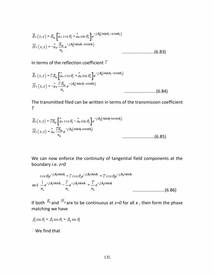
135

..........................(6.83)

In terms of the reflection coefficient

..........................(6.84)

The transmitted filed can be written in terms of the transmission coefficient T

..........................(6.85)

We can now enforce the continuity of tangential field components at the boundary i.e. z=0

..........................(6.86)

If both and are to be continuous at z=0 for all x , then form the phase matching we have

We find that

136

..........................(6.87)

Further, from equations (6.86) and (6.87) we have

..........................(6.88)

or ..........................(6.89)

..........................(6.90)

From equation (6.90) we find that there exists specific angle for which = 0 such that

or .........................(6.91)

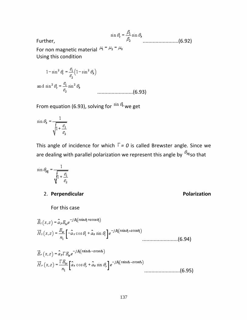
137

Further, .........................(6.92)

For non magnetic material Using this condition

.........................(6.93)

From equation (6.93), solving for we get

This angle of incidence for which = 0 is called Brewster angle. Since we

are dealing with parallel polarization we represent this angle by so that

2. Perpendicular Polarization For this case

.........................(6.94)

.........................(6.95)

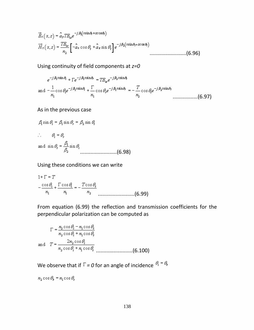
138

.........................(6.96)

Using continuity of field components at z=0

.................(6.97)

As in the previous case

.........................(6.98)

Using these conditions we can write

.........................(6.99)

From equation (6.99) the reflection and transmission coefficients for the perpendicular polarization can be computed as

.........................(6.100)

We observe that if = 0 for an angle of incidence

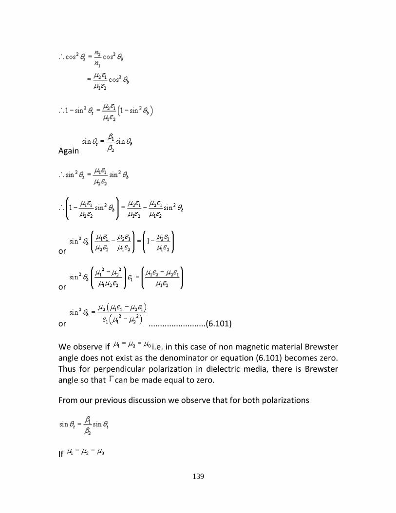
139

Again

or

or

or .........................(6.101)

We observe if i.e. in this case of non magnetic material Brewster angle does not exist as the denominator or equation (6.101) becomes zero. Thus for perpendicular polarization in dielectric media, there is Brewster angle so that can be made equal to zero.

From our previous discussion we observe that for both polarizations

If

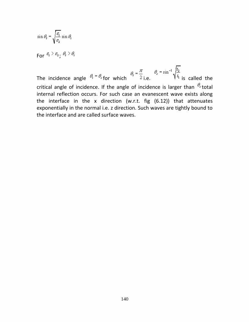
140

For ;

The incidence angle for which i.e. is called the

critical angle of incidence. If the angle of incidence is larger than total internal reflection occurs. For such case an evanescent wave exists along the interface in the x direction (w.r.t. fig (6.12)) that attenuates exponentially in the normal i.e. z direction. Such waves are tightly bound to the interface and are called surface waves.

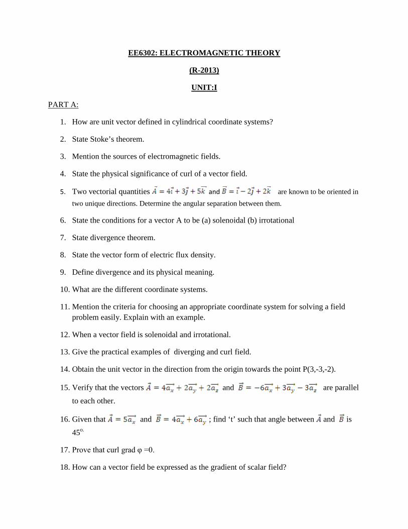
EE6302: ELECTROMAGNETIC THEORY

(R-2013)

UNIT:I

1. How are unit vector defined in cylindrical coordinate systems?

PART A:

2. State Stoke’s theorem.

3. Mention the sources of electromagnetic fields.

4. State the physical significance of curl of a vector field.

5. Two vectorial quantities and are known to be oriented in two unique directions. Determine the angular separation between them.

6. State the conditions for a vector A to be (a) solenoidal (b) irrotational

7. State divergence theorem.

8. State the vector form of electric flux density.

9. Define divergence and its physical meaning.

10. What are the different coordinate systems.

11. Mention the criteria for choosing an appropriate coordinate system for solving a fieldproblem easily. Explain with an example.

12. When a vector field is solenoidal and irrotational.

13. Give the practical examples of diverging and curl field.

14. Obtain the unit vector in the direction from the origin towards the point P(3,-3,-2).

15. Verify that the vectors and are parallel

to each other.

16. Given that and ; find ‘t’ such that angle between and is

45

17. Prove that curl grad φ =0.

o.

18. How can a vector field be expressed as the gradient of scalar field?

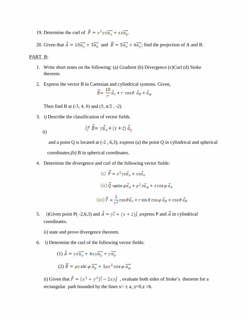
19. Determine the curl of .

20. Given that and ; find the projection of A and B.

PART B

1. Write short notes on the following: (a) Gradient (b) Divergence (c)Curl (d) Stoke theorem.

:

2. Express the vector B in Cartesian and cylindrical systems. Given,

Then find B at (-3, 4, 0) and (5, π/2 , -2)

3. i) Describe the classification of vector fields.

ii)

and a point Q is located at (-2 , 6,3), express (a) the point Q in cylindrical and spherical

coordinates,(b) B in spherical coordinates.

4. Determine the divergence and curl of the following vector fields:

=ρ

5. i)Given point P( -2,6,3) and ,express P and in cylindrical coordinates.

ii) state and prove divergence theorem.

6. i) Determine the curl of the following vector fields:

(1)

(2)

ii) Given that , evaluate both sides of Stoke’s theorem for a rectangular path bounded by the lines x= ± a, y=0,z =b.

7. i) Find the electric field at a point P(0,0,6) due to a point charge Q1 of 0.35 µC placedat (0,5,0) and Q2

ii) obtain in the spherical coordinate system the gradient of the function

of -0.6 µC placed at (5,0,0).

.

8. i) State and derive divergence theorem.

ii) show that in catesian coordinates for any vector A, .

9. Explain the different coordinate systems.

10. Write short notes on gradient,divergence, curl and stokes theorem.

UNIT:II

1. Define electrical potential

PART A:

2. Define potential differences.

3. Name few applications of Gauss law in electrostatics.

4. State the properties of electric flux lines.

5. A dielectric slap of flat surface with relative permittivity 4 is disposed with its surface normal to a uniform field with flux density 1.5c/m2

6. A parallel plate capacitor has a charge of 10

. The slab is uniformly polarized. Determine polarization in the slab.

-3

7. Define electric dipole.

c on each plate while the potential difference between the plates is 1000v. calculate the value of capacitance.

8. Define electric dipole moment.

9. Write Poissons equation for a simple medium

10. Write laplace equation for a simple medium.

11. Define dielectric strength.

12. What is meant by dielectric breakdown.

13. A uniform line charge with ρl =5 µC/m lies along the x-axis. Find at (3,2,1) m.

14. State the expression for polarization.

15. What are the boundary conditions between two dielectric media?

16. Write the continuity equation.

17. Define energy density.

18. Write the equation for capacitance of coaxial cable.

19. Write the equation for point from ohm’s law.

20. Distinguish between displacement and conduction currents.

1. Deduce an expression for the capacitance of parallel plate capacitor having two identical media.

PART B:

2. i) state and derive electric boundary condition for a dielectric to dielectric medium and a conductor to dielectric medium.

ii)Derive the expression for energy density in electrostatic fields.

3. (i)State and explain coulomb’s law and deduce the vector form of force equation between two point charges.

(ii)At an interface separating dielectric 1(εr1) and dielectric 2(εr2) show that the tangential component of is continuous across the boundary, whereas the normal component of is discontinuous at the boundary.

4. (i) A circular disc of radius ‘a’ m is charged uniformly with a charge density of ρsC/m2

ii) find the value of capacitance of a capacitor consisting of two parallel metal plates of 30cm x 30cm surface area, separately by 5mm in air. What is the total energy stored by capacitor is charged to a potential difference of 1000v? what is the energy density?

. Find the electric potential at a point P diatant ‘h’ m from the disc surface along its axis.

5. i)A circular disc of radius ‘a’ m is charged uniformly with a charge density of’σcoulombs/m2

ii)Determine the electric field density at P(-0.2,0, -2.3) due to a point charge of +5nC at Q(0.2, 0.1, -2.5) in air. All dimensions are in meter.

. Find the potential at a point ‘h’m from the disc surface along its axis.

6. Find the potential at any point along the axis of a uniformly charged disc of σ c/m2

7. Derive the expression for energy stored and energy density in electrostastic fields.

. The disc has radius of ‘a’ m

8. Derive the boundary conditions at the interface of two dielectrics.

9. Point charges 1 mC and -2 mC are located at (3,2,-1) and (-1, -1,4) respectively. Calculate the electric force on a 10nC charge located at (0,3,1) and the electric field intensity at the point.

10. A linear ,homogeneous , isotropic dielectric material has εr=3.6 and is covering the space

between z=0 and z=1. If v= -6000z volts in the material, find

UNIT:III

1. Write down the magnetic boundary conditions.

PART A:

2. What is Lorentz law of force?

3. Write the expression for magnetic field H at the centre of a circular coil carrying a current of I amperes. The radius of the coil is a m

4. State ohms law for magnetic circuits.

5. Write the expression for the magnetic force between an electromagnet and an armature to be attracted.

6. Find the inductance per unit length of a long solenoid of N turns and having a length L ‘mtrs’. Assume that it carries a current of I amperes.

7. State Ampere’s circuital law.

8. State Biot savarts law.

9. What is the expression for inductance of a toroid?

10. Define the terms: magnetic moment and magnetic permeability.

11. State the law of conservation of magnetic flux.

12. Define magnetostaic energy density.

13. Draw the BH curve for classifying magnetic materials.

14. Define vector magnetic potential.

15. Define self inductance and mutual inductance.

16. A current of 3A flowing through an inductor of 100mH. What is the energy stored in the inductor?

17. Distinguish between diamagnetic, paramagnetic and ferromagnetic materials.

18. Sketch Gauss law for the magnetic field.

19. Classify the magnetic material.

20. State the expression for H due to infinite sheet of current.

21. Write the expression for the torque experienced by a current carrying loop placed in the magnetic field.

1. State and explain Ampere’s circuit law and show that the field strength at the end of a long solenoid is one half of that at the centre.

PART B:

2. a) State and explain Bio-savarts law.

b)Derive an expression for the force between two long straight parallel current carrying conductors.

3. Derive a general expression for the magnetic flux density B at any point along the axis of a long solenoid. Sketch the variation of B from point to point along the axis.

4. i) For a finite current sheet of uniform current density ‘k’ A/m, Derive the expression for the magnetic field intensity.

ii)A coil has 1000 turns and carries a magnetic flux of 10mwb. The resistance of the coil is 4 ohm. If it is connected to a 40v DC supply estimate the energy stored in the magnetic field when the current has attained its final study value. Derive the formula used.

5. i) Show by means of Biot Savarts law that the flux density produced by an infinitely long straight wire carrying a current I at any point distant a normal to the wire is given by μ0 μr

ii)what is the maximum torque on a square loop of 1000turns in a field of uniform flux density B tesla? The loop has 10cm sides and carries a current of 3A . what is the magnetic moment of the loop?

I/2πa.

6. i)Derive Biot Savart’s law and ampere law using the concept of magnetic vector potential.

ii) The core of a toroid is of 12 cm2 area and is made of material with μr

7. i)Derive the expression for the magnetic field intensity inside and outside a co-axial conductor of inner radius ‘a’ and outer radius ‘b’ and carrying a current of I ampers in the inner and outer conductor.

=200. If the mean radius of the toroid is 50cm. Calculate the number of turns needed to obtain an inductance of 2.5H.

ii)Calculate the self inductance of infinitely long solenoid.

8. I)Derive the expression for the magnetic vector potential in the cases of an infinitely long straight conductor in free space.

ii)consider the boundary between two media. Show that the angles between the normal to the boundary and the conductivities on either side of the boundary satisfy the relation.

9. Obtain the expression for energy stored in the magnetic field and also derive the expression for magnetic energy density.

10. I)Derive the expression for coefficient of coupling in terms of mutual and self inductance of the coils

ii) An iron ring with a cross sectional area of 8cm2

11. Derive an expression for the force between two long straight parallel current carrying conductors.

and a mean circumference of 120cm iswound with 480 turns of wire carrying a current of 2 A. the relative permeability of the ring is 1250.Calculte the flux established in the ring.

UNIT –IV

1. State the faraday’s law.

PART-A

2. State the faraday’s law for the moving charge in a constant magnetic field.

3. State lenz’s law.

4. Define displacement current density.

5. What are electric field and the power flow in the co-axial cable?

6. Define reluctance.

7. Write the maxwell’s equation from ampere’s law both in integral and point forms.

8. Write down the maxwell’s equation from electric gauss’s law in integral and point forms.

9. Write the maxwell’s equation from faraday’s law both in integral and point forms.

10. Write down the maxwell’s equation from magnetic gauss’s law in integral and point form.

11. Write the maxwell’s equations from Gauss’s law in integral form.

12. Write to maxwell’s equations in integral form.

13. Write down the maxwell’s equations from Gauss’s law in point form.

14. Write down the maxwell’s equation in point from.

15. Write down the maxwell’s equation in point phasor forms.

16. Write down the maxwell’s equation for free space in integral form.

17. Explain why

18. Explain why XE=0

19. In material for which and and E=250 sin t (V/m) .Find the conduction and displacement current densities.

20. Explain why

PART – B

1. The magnetic field intensity in free space is given as H= H0 sin y A/m.Where = t - and is a constant quantity. Determine the displacement current density.

2. Show that the ratio of the amplitudes of the conduction current density and displacement current density is , for the applied E= Em cos Assume µ =µ0, what is the amplitude

ratio, if the applied field is E= Em .where is real?

3. Derive maxwell’s equation from ampere’s law in integral and point form.

4. Do the fields E= Em sin x. Sin t and = (Em/µ0) cosx cost z

5. State maxwell’s equations and obtain them in differential form. Also derive them harmonically varying field.

satisfy maxwell’s equations?

6. State maxwell’s equation and obtain them in integral and differential form.

7. Derive the maxwell’s equation in phasor integral form.

8. Derive the maxwell’s equation in phasor differential form.

9. If electric field intensity in free space is given by = (50/ ) COS (108 t- 10 z ) V/m . Find the magnetic field intensity .

10. State and derive the maxwell’s equations for free space in integral form and point form for time varying field.

UNIT – V

1. Define a wave.

PART –A

2. What are wave equations for free space?

3. What is a uniform plane wave?

4. What is the relationship between E and H or brief about intrinsic impedance for a dielectric medium?

5. What are Helmholtz equations or represent equation of electromagnetic wave in the phasor form?

6. What are the wave equations for a conducting medium?

7. What is phase velocity?

8. What are the values of in terms of primary constants of the medium?

9. Write down the secondary contants of a good conductor.

10. Write down the values of velocity and intrinsic impedance for free space.

11. What is skin effect?

12. Define skin depth or depth of penetration of a conductor.

13. Determine the skin depth of copper at 60 Hz with 5.8 X 107 s/m. Given r

14. What is polarization?

= 1.

15. Define linear, elliptical and circular polarization?

16. Define snell’s law of refraction.

17. Define critical angle.

18. Define Brewster angle.

19. What are the standing waves?

20. How a dielectric medium can be identified as lossless and lossy for a given frequency?

PART – B

1. Derive general wave equations in phasor form and also derive for .

2. Derive wave equations for a conducting medium.

3. State pointing theorem and derive an expression for pointing theorem.

4. Explain the wave propagation in good dielectrics with necessary equations.

5. Derive the expression for total magnetic field when a vertically polarized wave is incident obliquely on a perfect conductor.

6. Determine the reflection coefficient of oblique incidence in perfect dielectric for parallel polarization.

7. Determine the reflection coefficient of oblique incidence in perfect dielectric for perpendicular polarization.

8. Define polarization. What are the different types of wave polarization? Explain them with mathematical expression.

9. Obtain the expression for the reflection coefficient and transmission coefficient for a wave normally incident on the surface of a dielectric.

10. A uniform plane wave in a medium having 10-3 s/m, 80 0 and 0

i) Verify whether the medium is good conductor

is having a frequency of 10 KHz.

ii) Calculate the following,

1) Attenuation constant 2) Phase constant 3) Propagation constant 4) Intrinsic impedance 5) Wave length 6) Velocity of propagation