contentsmelvyn c branch*, university of colorado at boulder, hei health research committee steven...

CONTENTSHEI Communication 10

H E A L T HE F F E C T SINSTITUTE

PREFACE

HEI SYNTHESIS Introduction . . . . . . . . . . . . . . . . . . . . . . . . . . . . . . . . . 3Searching for the Diesel Signature . . . . . . . . . . . . . . 4

Epidemiologic Study Designs and Exposure Assessment Issues . . . . . . . . . . . . . . . . 4

What Are the Characteristics of the Ideal Diesel Exhaust Signature? . . . . . . . . . . . . . 5

Summary of Workshop Presentations . . . . . . . . . . 5Health Studies of Diesel

Particulate Matter . . . . . . . . . . . . . . . . . . . . . . . . . 5Future Trends of Diesel Emissions. . . . . . . . . . . . 6Diesel and Gasoline Particle

Characteristics . . . . . . . . . . . . . . . . . . . . . . . . . . . . 6Approaches to Particle

Characterization . . . . . . . . . . . . . . . . . . . . . . . . . . 6

Diesel Source Signature Studies . . . . . . . . . . . . . . 7Emissions and Air Quality Studies . . . . . . . . . . . . 8Data Analysis Approaches . . . . . . . . . . . . . . . . . . . 9

Do We Have a Diesel Signature? Where Do We Go from Here?. . . . . . . . . . . . . . . . . . 9

Epidemiologic Implications . . . . . . . . . . . . . . . . . 9Chemical Characterization Issues . . . . . . . . . . . 10Trying to Separate Diesel Emissions

from Spark-Ignition Engine Emissions. . . . . . 11Methods Development. . . . . . . . . . . . . . . . . . . . . 12Linking Disciplines . . . . . . . . . . . . . . . . . . . . . . . . 12

Conclusions and Research Directions. . . . . . . . . . 12References . . . . . . . . . . . . . . . . . . . . . . . . . . . . . . . . . . 14Abbreviations and Other Terms . . . . . . . . . . . . . . . 14

REPORTS FROM SPEAKERS

Health Studies of Diesel Particulate Matter

Exposure Assessment Issues in Epidemiology Studies on Chronic Health Effects of Diesel Exhaust Eric Garshick, Francine Laden, Jaime E Hart, and Thomas J Smith . . . . . . . . . . . . . . . . . . . . . . . . . . . . . . . . . . . . . . . . . . . . . . . . . . . . . . . . . . . . . . . . . . . . . .17

Issues in Exposure Assessment in Epidemiologic Studies of Acute Effects of Diesel Exhaust Patrick L Kinney. . . . . . . . . . . . . . . . . . . . . . . . . . . . . . . . . . . . . . . . . . . . . . . . . . . . . . . . .27

US EPA’s Health Assessment Document for Diesel Engine Exhaust Charles Ris . . . . . . . . . . . . . . . . . . .33

Future Trends of of Diesel Emissions

The Future of Diesel Emissions Robert F Sawyer . . . . . . . . . . . . . . . . . . . . . . . . . . . . . . . . . . . . . . . . . . . . . .39Difference Between Off-Road and On-Road Emissions Terry L Ullman . . . . . . . . . . . . . . . . . . . . . . . . .45

Diesel and Gasoline Particle Characteristics

Some Characteristics of Diesel and Gasoline Particulate Emissions David Kittelson . . . . . . . . . . . . . .51

Approaches to Particle Characterization

Morphological Aspects of Combustion Particles Douglas A Blom, John ME Story, and RL Graves. . . . . . . . . . . . . . . . . . . . . . . . . . . . . . . . . . . . . . . . . . . . . . . . . . . . . . . . . . . . . .57

Characterization of Vehicle Emissions and Urban Aerosols by an Aerosol Mass Spectrometer Douglas R Worsnop, Manjula Canagaratna, John Jayne, and Jose Jimenez . . . . . . . . . . . . . . . . . . . . . . . . . . . . . . . . . . . . . . . . . . . . . . . . . . . . . . . . . . . . . .63

On-Line Mass Spectral Analysis of Thermally Evaporated Diesel Exhaust Particles Paul J Ziemann, Herbert J Tobias, Hiromu Sakurai, Peter H McMurry and David B Kittelson . . . . . . . . . . . . . . . . . . . . . . . . . . . . . . . . . . . . . . . . . . . . . . . . . . . . . . . . . . . . . . . . . . . .73

Using Individual Particle Signatures to Discriminate Between HDV and LDV Emissions Sergio A Guazzotti and Kimberly A Prather . . . . . . . . . . . . . . . . . . . . . . . . . . . . . . . . . . .81

Continued

Diesel Source Signature Studies

Diesel Exhaust Signatures for Source Attribution: Part 1 James J Schauer . . . . . . . . . . . . . . . . . . . . . . . 93Diesel Exhaust Signatures for Source Attribution: Part 2 James J Schauer . . . . . . . . . . . . . . . . . . . . . . 101Chemical Characterization of On-Road Motor Vehicle PM Emissions

Eric Fujita and Barbara Zielinska . . . . . . . . . . . . . . . . . . . . . . . . . . . . . . . . . . . . . . . . . . . . . . . . . . . . . . . . 103

Emissions and Air Quality Studies

A Brief Summary of DOE’s Gasoline/Diesel PM Split Study Douglas R Lawson . . . . . . . . . . . . . . . . . 111Particulate Matter from Gasoline Engines Chad R Bailey, Carl R Fulper,

Richard W Baldauf, and Joseph H Somers . . . . . . . . . . . . . . . . . . . . . . . . . . . . . . . . . . . . . . . . . . . . . . . . . 121Historical Efforts at Source Apportionment Philip K Hopke . . . . . . . . . . . . . . . . . . . . . . . . . . . . . . . . . . 129Estimates of Diesel and Other Emissions: Overview of the Supersite Program

Spyros N Pandis . . . . . . . . . . . . . . . . . . . . . . . . . . . . . . . . . . . . . . . . . . . . . . . . . . . . . . . . . . . . . . . . . . . . . . . . 135Contribution of Local Versus Regional Sources to Exposure

Constantinos Sioutas . . . . . . . . . . . . . . . . . . . . . . . . . . . . . . . . . . . . . . . . . . . . . . . . . . . . . . . . . . . . . . . . . . . 143

Data Analysis Approaches

Data Analytic Approaches for Monitoring Specific Pollutants in Epidemiological Studies Richard L Smith. . . . . . . . . . . . . . . . . . . . . . . . . . . . . . . . . . . . . . . . . . . . . . . . . . . . . . . . . . . . . . . . . 153

Appendix. Workshop Agenda

Publishing History: This document was posted as a preprint on www.healtheffects.org and then finalized for print.Citation for whole report:

Health Effects Institute. 2003. Improving Estimates of Diesel and Other Emissions for Epidemiologic Studies.Communication 10. Health Effects Institute, Boston MA.

When specifying a section of this Communication, cite it as a chapter of this document.

C O M M U N I C A T I O N 1 0

Improving Estimates of Diesel and OtherEmissions for Epidemiologic Studies

April 2003

H E A L T HE F F E C T SINSTITUT E

Proceedings of an HEI Workshop Baltimore, MarylandDecember 4 to 6, 2002

Contributors

Writing Team Maria G Costantini*, Health Effects InstituteDebra A Kaden*, Project Leader, Health Effects Institute Armistead G Russell*, Georgia Institute of TechnologyJonathan Samet*, Johns Hopkins Bloomberg School of Public Health, HEI Health Research CommitteeJane Warren*, Health Effects Institute

Administrative Staff Terésa Fasulo, Workshop Coordinator, Health Effects InstituteMelissa Harke, Health Effects Institute

PublicationsGenevieve MacLellan, Consulting EditorCarol Moyer, Consulting EditorRuth Shaw, CameographicsJenny Lamont, Health Effects InstituteSally Edwards, Health Effects Institute

Advisory GroupArmistead G Russell*, Georgia Institute of Technology; Chair, Workshop Planning GroupNicholas J Barsic*, John DeereMelvyn C Branch*, University of Colorado at Boulder, HEI Health Research CommitteeSteven Cadle*, General Motors CorporationKenneth L Demerjian,* State University of New York at Albany, HEI Health Research CommitteeEric Fujita, Desert Research InstituteEric Garshick, Brigham and Women’s HospitalRogene Henderson, Lovelace Respiratory Research Institute, HEI Health Research CommitteePatrick Kinney, Columbia UniversityDavid B Kittelson*, University of MinnesotaMichael Kleeman, University of California, DavisDouglas Lawson, National Renewable Energy LaboratoryThomas A Louis*, Johns Hopkins Bloomberg School of Public Health, HEI Health Review CommitteeEileen McCauley, California Air Resource BoardJonathan Samet*, Johns Hopkins Bloomberg School of Public Health, HEI Health Research CommitteeRobert F Sawyer*, University of California, Berkeley; Chair, HEI Special Committee on Emerging TechnologiesJames Schauer, University of WisconsinRichard Smith, University of North Carolina, Chapel HillJoseph H Somers*, US Environmental Protection AgencyBarbara Turpin, Rutgers UniversityDouglas Worsnop, Aerodyne Research Barbara Zielinska, Desert Research Institute

* Workshop Planning Group members.

Improving Estimates of Diesel and Other Emissionsfor Epidemiologic Studies

Proceedings of an HEI WorkshopDecember 4 to 6, 2002Baltimore, Maryland

In Memory of Glen Cass

This Workshop Report is dedicated to Glen Cass, an eminent air pollution scientist and teacher who, as amember of HEI’s Health Research Committee, made extraordinary contributions to HEI’s research program.Professor Cass was a leading figure in the development of molecular methods for identifying sources of airpollution, a research area relevant to identifying specific markers for diesel exhaust, the subject of thisworkshop. He trained a cadre of scientists and engineers who are now applying those methods in many placesand rapidly advancing the methods and knowledge. Several of his former students contributed to thisworkshop. Professor Cass passed away in 2001, leaving a tremendous legacy of accomplishments in manyareas of air pollution research and numerous scientists who will continue his work.

CONTENTSHEI Communication 10

H E A L T HE F F E C T SINSTITUTE

PREFACE

HEI SYNTHESIS Introduction . . . . . . . . . . . . . . . . . . . . . . . . . . . . . . . . . 3Searching for the Diesel Signature . . . . . . . . . . . . . . 4

Epidemiologic Study Designs and Exposure Assessment Issues . . . . . . . . . . . . . . . . 4

What Are the Characteristics of the Ideal Diesel Exhaust Signature? . . . . . . . . . . . . . 5

Summary of Workshop Presentations . . . . . . . . . . 5Health Studies of Diesel

Particulate Matter . . . . . . . . . . . . . . . . . . . . . . . . . 5Future Trends of Diesel Emissions. . . . . . . . . . . . 6Diesel and Gasoline Particle

Characteristics . . . . . . . . . . . . . . . . . . . . . . . . . . . . 6Approaches to Particle

Characterization . . . . . . . . . . . . . . . . . . . . . . . . . . 6

Diesel Source Signature Studies . . . . . . . . . . . . . . 7Emissions and Air Quality Studies . . . . . . . . . . . . 8Data Analysis Approaches . . . . . . . . . . . . . . . . . . . 9

Do We Have a Diesel Signature? Where Do We Go from Here?. . . . . . . . . . . . . . . . . . 9

Epidemiologic Implications . . . . . . . . . . . . . . . . . 9Chemical Characterization Issues . . . . . . . . . . . 10Trying to Separate Diesel Emissions

from Spark-Ignition Engine Emissions. . . . . . 11Methods Development. . . . . . . . . . . . . . . . . . . . . 12Linking Disciplines . . . . . . . . . . . . . . . . . . . . . . . . 12

Conclusions and Research Directions. . . . . . . . . . 12References . . . . . . . . . . . . . . . . . . . . . . . . . . . . . . . . . . 14Abbreviations and Other Terms . . . . . . . . . . . . . . . 14



Exposure Assessment Issues in Epidemiology Studies on Chronic Health Effects of Diesel Exhaust Eric Garshick, Francine Laden, Jaime E Hart, and Thomas J Smith . . . . . . . . . . . . . . . . . . . . . . . . . . . . . . . . . . . . . . . . . . . . . . . . . . . . . . . . . . . . . . . . . . . . . .17

Issues in Exposure Assessment in Epidemiologic Studies of Acute Effects of Diesel Exhaust Patrick L Kinney. . . . . . . . . . . . . . . . . . . . . . . . . . . . . . . . . . . . . . . . . . . . . . . . . . . . . . . . .27

US EPA’s Health Assessment Document for Diesel Engine Exhaust Charles Ris . . . . . . . . . . . . . . . . . . .33

Future Trends of of Diesel Emissions

The Future of Diesel Emissions Robert F Sawyer . . . . . . . . . . . . . . . . . . . . . . . . . . . . . . . . . . . . . . . . . . . . . .39Difference Between Off-Road and On-Road Emissions Terry L Ullman . . . . . . . . . . . . . . . . . . . . . . . . .45

Diesel and Gasoline Particle Characteristics

Some Characteristics of Diesel and Gasoline Particulate Emissions David Kittelson . . . . . . . . . . . . . .51

Approaches to Particle Characterization

Morphological Aspects of Combustion Particles Douglas A Blom, John ME Story, and RL Graves. . . . . . . . . . . . . . . . . . . . . . . . . . . . . . . . . . . . . . . . . . . . . . . . . . . . . . . . . . . . . .57

Characterization of Vehicle Emissions and Urban Aerosols by an Aerosol Mass Spectrometer Douglas R Worsnop, Manjula Canagaratna, John Jayne, and Jose Jimenez . . . . . . . . . . . . . . . . . . . . . . . . . . . . . . . . . . . . . . . . . . . . . . . . . . . . . . . . . . . . . .63

On-Line Mass Spectral Analysis of Thermally Evaporated Diesel Exhaust Particles Paul J Ziemann, Herbert J Tobias, Hiromu Sakurai, Peter H McMurry and David B Kittelson . . . . . . . . . . . . . . . . . . . . . . . . . . . . . . . . . . . . . . . . . . . . . . . . . . . . . . . . . . . . . . . . . . . .73

Using Individual Particle Signatures to Discriminate Between HDV and LDV Emissions Sergio A Guazzotti and Kimberly A Prather . . . . . . . . . . . . . . . . . . . . . . . . . . . . . . . . . . .81

Continued


Diesel Exhaust Signatures for Source Attribution: Part 1 James J Schauer . . . . . . . . . . . . . . . . . . . . . . . 93Diesel Exhaust Signatures for Source Attribution: Part 2 James J Schauer . . . . . . . . . . . . . . . . . . . . . . 101Chemical Characterization of On-Road Motor Vehicle PM Emissions

Eric Fujita and Barbara Zielinska . . . . . . . . . . . . . . . . . . . . . . . . . . . . . . . . . . . . . . . . . . . . . . . . . . . . . . . . 103

Emissions and Air Quality Studies

A Brief Summary of DOE’s Gasoline/Diesel PM Split Study Douglas R Lawson . . . . . . . . . . . . . . . . . 111Particulate Matter from Gasoline Engines Chad R Bailey, Carl R Fulper,

Richard W Baldauf, and Joseph H Somers . . . . . . . . . . . . . . . . . . . . . . . . . . . . . . . . . . . . . . . . . . . . . . . . . 121Historical Efforts at Source Apportionment Philip K Hopke . . . . . . . . . . . . . . . . . . . . . . . . . . . . . . . . . . 129Estimates of Diesel and Other Emissions: Overview of the Supersite Program

Spyros N Pandis . . . . . . . . . . . . . . . . . . . . . . . . . . . . . . . . . . . . . . . . . . . . . . . . . . . . . . . . . . . . . . . . . . . . . . . . 135Contribution of Local Versus Regional Sources to Exposure

Constantinos Sioutas . . . . . . . . . . . . . . . . . . . . . . . . . . . . . . . . . . . . . . . . . . . . . . . . . . . . . . . . . . . . . . . . . . . 143

Data Analysis Approaches

Data Analytic Approaches for Monitoring Specific Pollutants in Epidemiological Studies Richard L Smith. . . . . . . . . . . . . . . . . . . . . . . . . . . . . . . . . . . . . . . . . . . . . . . . . . . . . . . . . . . . . . . . . 153

Appendix. Workshop Agenda

Publishing History: This document was posted as a preprint on www.healtheffects.org and then finalized for print.Citation for whole report:

Health Effects Institute. 2003. Improving Estimates of Diesel and Other Emissions for Epidemiologic Studies.Communication 10. Health Effects Institute, Boston MA.

When specifying a section of this Communication, cite it as a chapter of this document.

PREFACE

Health Effects Institute Communication 10 © 2003 1

Diesel engines are used extensively in heavy-duty trans-portation applications due to their power and durability.Due to their increased fuel efficiency as compared to gaso-line vehicles, diesel engines are also finding worldwideapplication in light-duty vehicles. Fuel efficiency andlower emissions of the greenhouse gas carbon dioxide perunit of work also offer advantages over gasoline from thepoint of view of global warming. These issues will becomeincreasingly important as the number of vehicle-milestraveled increases around the world. The major concernabout diesel engines has been their high emissions of par-ticulate matter (PM) and nitrogen oxides. Over the pastdecade, engine manufacturers have significantly loweredPM emissions from diesel engines by improving enginetechnologies and adding after-treatment technologies. Fur-ther efforts aim to decrease PM and nitrogen oxide fromdiesel engines to meet the 2004 and 2007 diesel standards.

Several state, national, and international agencies haveconcluded that diesel exhaust is a probable human carcin-ogen, citing as evidence the occupational epidemiologicstudies associating diesel exhaust exposure with lungcancer and some support from animal studies. In order toestimate the potential public health significance, someagencies have developed quantitative risk estimates. How-ever, difficulty in accurately estimating occupationalexposure in the studies from which these risk estimates arederived limits interpretation of the epidemiologic evi-dence and its application to quantitative risk assessment.Thus, improved exposure assessment is necessary forcharacterizing both short-term and long-term health effectsof exposure to diesel exhaust.

In 1998, HEI initiated its Diesel Epidemiology Project, aresearch and assessment effort aimed at (1) understandingthe strengths and limitations of using published epidemio-logic data in quantitative risk assessment of diesel exposureand lung cancer; and (2) funding feasibility studies to iden-tify new diesel-exposed cohorts and to improve exposureassessment methods. The feasibility studies would ulti-mately lead to full epidemiologic studies aiming to providesharper characterization of the exposure–risk relation.

The Diesel Epidemiology Expert Panel was appointed toconduct a systematic review of epidemiologic studies ofdiesel exposure and lung cancer and to assess their utilityfor quantitative risk assessment. The Panel concluded thatlarger epidemiologic studies of cohorts with reasonablycharacterized exposures were needed for quantitative riskassessment and that further exploration of existing studies

or the development of new studies could provide betterdata for risk assessment (Diesel Epidemiology ExpertPanel 1999). The Panel recommended that HEI considerundertaking a new epidemiologic study if its feasibilitystudies identified suitable cohorts particularly if existingexposure assessment methods were sufficiently accurate.

In the fall of 2000, the Diesel Epidemiology WorkingGroup was formed to continue the work of the Diesel Epide-miology Expert Panel. It was charged with (1) reviewingreports from 6 feasibility studies funded by HEI, and (2)developing an agenda for research that would provide betterinformation for assessing quantitative risk from diesel expo-sure and adverse health effects, including lung cancer.

In its report, the Diesel Epidemiology Working Group(2002) concluded that full studies of cohorts that had beencharacterized in the feasibility studies would not generatesubstantially more accurate exposure–response informa-tion. The Working Group also concluded from the feasi-bility studies that the available methods for assessingexposure to diesel exhaust were not sufficiently specific.Working Group members agreed with several investigatorsin their finding that elemental carbon may be a usefulmarker for occupational exposure to diesel exhaust if dieselengines are the dominant source of particles. The WorkingGroup noted, however, that elemental carbon by itself lacksthe necessary sensitivity and specificity to serve as a signa-ture of diesel exhaust in ambient exposure settings, whereparticles typically include elemental carbon from othercombustion sources. Therefore, they recommended identi-fying more specific markers, or a set of markers (a signa-ture), for diesel exhaust that could be used to enhanceexposure assessment for past studies, strengthen future epi-demiologic studies, and assess population exposures.

The Diesel Epidemiology Working Group did not recom-mend undertaking new cohort studies of the proposed pop-ulations characterized in the feasibility studies until furtherresearch has improved exposure assessment. The WorkingGroup identified activities that could enhance diesel riskassessment over the short, medium, and long term. The pro-posed short-term activities focused mainly on exposureassessment method. A workshop was recommended to dis-cuss the prospects for developing more informativemethods and better emissions and atmospheric data,including the potential for a sufficiently accurate signatureof diesel emissions, enhanced methods for characterizingparticles, and approaches for data analysis. The resultingHEI Workshop to Improve Estimates of Diesel and Other

2

Preface

Emissions for Epidemiologic Studies was held in Baltimorefrom December 4 to 6, 2002. This report summarizes thepresentations at the workshop and provides conclusionsfrom the workshop that identify possible research direc-tions for HEI and others interested in developing signaturesfor diesel and other combustion emissions.

REFERENCES

Diesel Epidemiology Expert Panel. 1999. Diesel Emissionsand Lung Cancer: Epidemiology and Quantitative RiskAssessment. Special Report. Health Effects Institute, Cam-bridge MA.

Diesel Epidemiology Working Group. 2002. ResearchDirections to Improve Estimates of Human Exposure andRisk from Diesel Exhaust. Special Report. Health EffectsInstitute, Boston MA.


HEI SYNTHESIS

INTRODUCTION

Particulate matter is a complex mixture of particles fromdifferent sources (both anthropogenic and natural) and withvarying size and composition. Indices of particulate matter(PM*) in outdoor air, as well as other indicators of combus-tion emissions such as elemental carbon (EC), have beenassociated with adverse health effects in epidemiologicstudies of a variety of designs, including time-series studiesof morbidity and mortality. Studies that have incorporatedcrude measures of exposure to vehicle emissions have alsofound associations between those exposure measures andincreased risk of adverse health effects. For the purpose ofair pollution control, an understanding of the toxicity of themany components of atmospheric PM is needed, along withmethods to trace the components exerting toxicity back totheir sources. There is substantial research in progress toidentify the characteristics of particles that may pose risksto health and the sources of these damaging particles. TheNational Research Council's Committee on Research Priori-ties for Airborne Particulate Matter has given high priorityto these topics (National Research Council 1998). There issome indication of heterogeneity in the effects of air pollu-tion across the United States, as shown, for example, in themaps of mortality effects based on the National Morbidity,Mortality, and Air Pollution Study (NMMAPS) (Samet et al2000a,b; Dominici et al 2003).

To identify the roles of different sources of PM in its tox-icity, epidemiologic studies need to incorporate exposuremeasures (indices) that have sufficient specificity to beinformative on the risks of the particles’ components orphysicochemical properties and also have some linkages tothe sources of the particles. Thus far, epidemiologicresearchers and exposure assessors have been unsuccessfulin identifying a sufficiently specific and sensitive marker ofdiesel exhaust exposure. Some individual components ofPM such as EC have been used as indicators of exposure todiesel exhaust. However, EC lacks the sensitivity and speci-ficity needed to be a marker of diesel emissions in the gen-eral ambient environment. In most urban locations,particularly in the United States, diesel emissions are onlyone contributor to a complex pollution mixture, and there

are generally other combustion sources of EC. A similarlimitation applies to other potential diesel markers,including certain volatile and semivolatile organic com-pounds.

HEI has identified the development of validatedmarkers or a set of markers (a signature) for diesel exhaustas an important short-term research need. Such a signaturemight be used to enhance exposure assessment for paststudies, depending on data and sample availability, wouldbe applicable to population exposure assessments, andcould also strengthen future epidemiologic studies. Toaddress this research need, HEI held the Workshop toImprove Exposure Estimates of Diesel and Other Emis-sions for Epidemiologic Studies, in early December 2002in Baltimore, Maryland. The workshop (agenda in theAppendix) had several goals:

• identify components of diesel exhaust that might be used as signatures;

• identify previously collected data and data currently being collected that could be further analyzed for this purpose;

• specify other measurements that might be useful in ongoing or planned studies; and

• address approaches to data exploration that might identify signatures.

The workshop brought together experts in emissionscharacterization, air pollution measurement, health effectsanalysis, data analysis, and risk assessment. Presentationsreviewing approaches for determining personal exposureto diesel exhaust in epidemiologic studies, as well as theirlimitations, were followed by results of current studiescharacterizing emissions from diesel (and other) sourcesand descriptions of methodologic approaches to identi-fying a diesel signature. These included characterizationof particle-bound organic compounds, single-particle massspectrometry analysis, and morphologic examination ofparticles. Participants also discussed how emissions data,together with ambient measurements, have been used forsource apportionment and the statistical methodologiesthat might be used to analyze these data in epidemiologicstudies of the effects of exposure to diesel exhaust. Fol-lowing the workshop, the Advisory Group, composed ofmembers of the Workshop Planning Group and otherexperts, met to discuss what could be concluded from theworkshop and the best directions for future research.

* A list of abbreviations and other terms appears at the end of the Synthesis.

This document has not been reviewed by public or private party institu-tions, including those that support the Health Effects Institute; therefore, itmay not reflect the views of these parties, and no endorsements by themshould be inferred.

4

HEI Synthesis

SEARCHING FOR THE DIESEL SIGNATURE

The handwritten signature of our own name is generallyunique and not readily replicated by others. The unique-ness of a signature lies in its individual letters and the waythat each is written. While handwriting might not makeany particular letter unique, their combination into anentire signature is almost always unique and becomesincreasingly so as the number of letters increases. Theuniqueness of a signature is useful in identifying an indi-vidual. Similarly, a signature would prove useful for iden-tifying exposure to diesel exhaust.

A principal limitation of epidemiologic studies of dieselexhaust exposure, whether of short-term or long-termeffects, has been bias from potential exposure misclassifi-cation. Even in the occupational studies of workers exposedto diesel exhaust, exposure misclassification has been a sub-stantial constraint in interpreting findings, making infer-ences with regard to associations between exposure andadverse health effects, and understanding expo-sure-response relations. The pattern of potential exposuremisclassification varies with the epidemiologic studydesign used. In cohort studies, thus far used primarily toassess occupational exposure and lung cancer, higherexposures that occurred in the more distant past have gen-erally been classified with less accuracy. In case-controlstudies, again primarily directed at lung cancer, there is apotential for differences in the reporting and estimation ofexposures for case subjects with lung cancer and for con-trol subjects without lung cancer. In cross-sectionalstudies, used for assessing nonmalignant respiratoryeffects (asthma exacerbation, excess decline in lung func-tion, and respiratory symptoms and morbidity in general),reporting of exposure may be influenced by a subject’s dis-ease status, possibly leading to inflated estimates of theeffect of exposure.

These same health effects—lung cancer, asthma, andrespiratory morbidity—remain of interest as a focus forcurrent research. Among the principal research issues arethe following:

• Is it possible to accurately measure diesel exposure so that quantitative estimates of the risk of lung cancer associated with diesel exposure can be made?

• Does diesel exposure contribute to allergic sensitiza-tion and exacerbation of asthma?

• Do diesel particles contribute to the health risks of PM generally?

Understanding the possible health effects of dieselexhaust has been a topic of investigation for severaldecades. Although diesel exhaust and diesel exhaust

particles have now been classified as probable carcinogens,the quantitative risk of lung cancer associated withexposure to diesel particles remains poorly characterized.In order to produce reliable exposure-response informationfor quantitative risk assessment, more specific measures ofexposure are needed.

Another issue of rising interest is the risk of asthma exac-erbation and allergic sensitization from diesel exhaust expo-sure. Experimental studies have found enhanced allergicresponse associated with diesel exposure, and observationalstudies have linked respiratory health indicators, includingasthma and wheezing, to the proximity of subjects’ resi-dences to roadways or high-traffic areas. However, theexperimental studies used high, and sometimes unrealistic,exposure conditions, and the observational studies usedcrude estimates of exposure and often lacked informationon other potential risk factors and confounding factors. Nev-ertheless, in the United States some neighborhoods, partic-ularly in inner cities, have substantial diesel traffic, andconcern has been raised that the resulting diesel exposuremay exacerbate asthma symptoms.

EPIDEMIOLOGIC STUDY DESIGNS AND EXPOSURE ASSESSMENT ISSUES

In studies considering the potential application of a sig-nature, the study design must be appropriate to addressthe given hypothesis. For example, in lung cancer studies,worker cohorts with higher levels of exposure enhance thepotential to describe exposure-response relations. Instudying the worker cohorts, the general approach shouldbe to develop a matrix of exposure estimates defined bytime periods and job periods for workers. Case-controlstudies are typically carried out in the general populationand usually incorporate job-exposure matrices for expo-sure estimates based on literature review and industrialhygiene assessments of likely levels of exposure. Retro-spective exposure assessment for diesel exhaust is furthercomplicated by the changing nature of the exhaust.

Hypotheses related to asthma and allergic diseases arebeing tested in cohort studies, including some studies thatstart with cohorts of newborns, and in cross-sectionalstudies. There are constraints on the number of measure-ments that can be made in such studies, and estimatingexposures is a greater challenge in the general populationsetting than in workplace settings, which typically havehigher exposures to diesel emissions. Furthermore, rela-tively fine time scales of exposure may be needed to assessexacerbation of asthma.

A variety of approaches might be used for exposure assess-ment in studies of workers and in studies of the general pop-ulation. A hierarchical or nested approach would generally

5

Communication 10

be preferable, in which the least invasive and most feasibleapproach would be used for the full set of participants, andthat approach would be validated by using increasinglyrefined measures in a nested fashion. Biomarkers specific todiesel exhaust have been sought, but none of sufficient spec-ificity has yet been identified.

As mentioned, error in measuring exposure is of con-cern. In general, imperfect measurements of diesel expo-sure will bias estimates of effect downward, therebyreducing the sensitivity of investigations to identifyadverse effects and to quantify risks with precision. Therehave also been temporal trends of reduced diesel exposureduring periods when measurement of exposure improved.This pattern can introduce subtle time-dependent biases.The challenge of addressing hypotheses related to possiblehealth effects of diesel exhaust is further complicated byvariation in the source characteristics over time (long termand short term) and space. Both the composition of dieselemissions and the resulting concentrations can change.Moreover, in the general environment, particles and gasesfrom diesel emissions are only one set of components of acomplex mixture that may include particles from othersources with similar characteristics and toxicity.

WHAT ARE THE CHARACTERISTICS OF THE IDEAL DIESEL EXHAUST SIGNATURE?

Characteristics of the ideal signature for diesel emis-sions would include (1) specificity for diesel exhaust, (2)feasibility of measurement, (3) possibility of being gener-ated from routinely collected data, (4) appropriate cost,and (5) relative insensitivity to engine technology and fuel.To find such a signature, we will need to sift throughalready collected data using exploratory approaches.There are substantial emissions characterization data thatcould be used to guide analyses of detailed data on atmo-spheric particles that have already been collected. Thesedata are especially valuable when ambient samples arecollected concurrently with source samples. Appropriateapproaches to exploratory data analysis are already avail-able. Ideally, protocols would be standardized to build aresource for future analysis.

SUMMARY OF WORKSHOP PRESENTATIONS

HEALTH STUDIES OF DIESEL PARTICULATE MATTER

Epidemiologic studies of populations exposed to dieselemissions at work or in the general environment rely on sur-rogate measures for exposure. These have included suchgeneral measures as distance of roadways from and trafficdensity near the subjects' residences for environmentalexposures, and job descriptions with industrial hygienemeasurements for occupational exposures, as well as poten-tial markers such as EC or black smoke. However, all ofthese surrogate measures also reflect other combustionsources, weakening the observed associations. Eric Garshickand Patrick Kinney presented some of the issues inassessing exposure in epidemiologic studies, including thecomplex nature of diesel exhaust, the multiple sources ofmany of the commonly used diesel markers, and the diffi-culty in linking the markers to an epidemiologic database,in terms of both current exposure and historical exposures.Although a single chemical marker for diesel exhaust wouldbe ideal for use in epidemiologic studies, experience sug-gests that a combination of multiple physical and chemicalmarkers will be necessary to distinguish between dieselexhaust and emissions from other combustion sources.Such signatures hold more promise for studies of chronicexposures (as opposed to acute exposures), which have typ-ically used central monitoring data for estimating expo-sures. Given the considerable spatial heterogeneity ofemissions, achieving sufficient detail across fine strata ofspace and time seems difficult at present.

Approaches to Assessing Diesel Exposure

Worker Cohort Studies

Historical measurements of particlesCurrent measures of particles and other indicatorsJob-exposure matrixBiomarkers of current or recent exposure

Case-Control Studies

Residence history• Proximity to roadways or other sources• Geographic information system approachesOccupational history• Job-exposure matrix

Cross-Sectional Studies

Residence location or history• Proximity to roadways or sources• Geographic information system approachesExposure monitoring• Regulatory monitoring for particles, nitrogen dioxide• Targeted monitoring for particles and other indicators• Area monitoring• Personal monitoring

6

HEI Synthesis

Charles Ris presented a summary of the recent US Envi-ronmental Protection Agency (EPA 2002) Health Assess-ment Document for Diesel Exhaust. Included in thisdocument are a characterization of diesel emissions and asummary of available information on dosimetry, mutage-nicity, noncancer effects (following both acute and chronicexposures), and cancer effects. Because of the level ofuncertainty associated with the exposure-response data,EPA did not provide a quantitative risk assessment fordiesel exhaust. Rather, it offered a range of estimates forthe possible lung cancer risk associated with environ-mental exposures to diesel exhaust. Recognizing that newtechnologies being developed and implemented will sub-stantially reduce the levels of emissions, EPA emphasizedthat the assessment was based on emissions from dieselengines built prior to the mid-1990s.

FUTURE TRENDS OF DIESEL EMISSIONS

Robert Sawyer discussed anticipated changes in dieselemissions. Many of the advanced engine technologies andexhaust gas aftertreatments under development are drivenby stricter standards for PM and oxides of nitrogen (NOX),which will begin in 2004 for light-duty diesel vehicles andin 2007 for heavy-duty vehicles. Emission standards arealso being phased in for nonroad engines, but these are lessstrict than those for on-road vehicles. The final controlsystem will likely include both a NOx catalyst (or NOxadsorber) and a particulate trap and will use fuel with verylow sulfur content (also required by law). Sawyer esti-mated that nonroad vehicles and pre-2007 heavy-dutyon-road vehicles will dominate diesel particulate emis-sions for the next 30 years. It is also likely that there will beincreased use of light-duty diesel vehicles (includingdiesel sport utility vehicles and vans) as a means toimprove fuel economy.

Terry Ullman summarized the history of emission regu-lations relative to on-road and off-road engines. The firstrule covering on-road diesel emissions was issued in 1979,and emission standards have become progressively morestringent; however, the regulation of emissions fromoff-road engines has lagged behind. As Robert Sawyer alsoindicated, the phase-in of off-road emission standardsbegan in 1996. On-road and off-road engines are testedusing different test cycles and fuels with different sulfurcontents. Generally, emissions of PM, NOx, and severalpolycyclic aromatic hydrocarbons (PAHs) are higher fromoff-road than from on-road vehicles. As on-road emissionsfurther decrease as a result of the 2004 and 2007 regula-tions, soot emissions (defined here as the PM mass minusthe soluble organic fraction) will be more strongly corre-lated to off-road emissions, and a combination of soot and

selected PAHs (for example, chrysene and naphthalene)may be used to identify emissions from off-road vehicles.

DIESEL AND GASOLINE PARTICLE CHARACTERISTICS

David Kittelson provided an overview of PM emissionsfrom diesel and gasoline engines. Particles from these typesof engines are similar in terms of both composition and sizedistribution. The particle size distribution is generallybimodal, with a nucleation mode (particles ranging in diam-eter from 3 to 30 nm) and an accumulation mode (particlesranging in diameter from 30 to 500 nm). Nuclei mode parti-cles consist of volatile and semivolatile compounds (mainlyorganic compounds and sulfate) and some solid material(metallic ashes and carbon) and are formed during dilutionand cooling of the exhaust. Particles in this mode are verysensitive to sampling conditions, such as dilution ratio andtemperature. The size of the volatile nuclei mode particlesis also dependent on the fuel sulfur content, but the relationbetween sulfur level and particle size is complex. Onehypothesis proposes that the presence of sulfur facilitatesnucleation and growth of particles made of heavy hydrocar-bons. Accumulation mode particles are composed primarilyof carbonaceous material and adsorbed components(organic compounds, sulfate, and metallic ash). They ariseinside the engine and are, therefore, sensitive toengine-operating conditions. This mode is generally notaffected by fuel sulfur content. The organic component ofthe diesel particles in both modes appears to be mainlyunburned lubricating oil. Most of the particle mass fromdiesel engines is found in the accumulation mode, while theparticle number represents both nuclei and accumulationmode particles. Future diesel engines will be very differentfrom current engines because of the need to introduce newtechnologies to further reduce NOx and PM and the wide-spread use of low-sulfur diesel fuel. As a consequence, par-ticle size distribution and composition will change.

APPROACHES TO PARTICLE CHARACTERIZATION

Douglas Blom described the use of transmission elec-tron microscopy to characterize the morphology of parti-cles collected from in-use diesel and gasoline vehicles.The technique uses particles collected by impaction on avery thin (electron-transparent) amorphous carbon film.Generally, carbonaceous particles from both diesel andgasoline combustion processes appear similar morpholog-ically (with chains of primary carbon particles). In the caseof diesel and traditional gasoline vehicles, the primaryparticles are typically between 30 and 60 nm in diameter.However, the primary particles from advanced-technologygasoline engines were found in two modes with one mode

7

Communication 10

comprising spheres of 10 nm in diameter while the otherparticles are more similar to traditional gasoline and dieselparticles (30–60 nm).

The aerosol mass spectrometer (AMS) represents a rela-tively new technique that permits detailed analysis of par-t ic le composit ion. The instrument samples andconcentrates particles using a high vacuum. The particlebeam is then directed to the ionization region, where vola-tile components of the particles are vaporized and ionized.The resulting ions are analyzed by the mass spectrometer,yielding a distinct mass spectrum that provides a detaileddescription of the aerosol sample. This technique can alsobe used to analyze the compositions of fuels and lubricatingoil. Both positive ions (such as organic species and metals)and negative ions (such as nitrates, sulfates, phosphate,chloride, organic compounds, and metal oxides) are gener-ally detected by the mass spectrometer. The AMS can beoperated in time-of-flight (TOF) mode to measuresize-dependent composition (by separating the particlesusing a beam-chopping technique) or in the mass spectrom-eter mode to provide spectra over the integrated size distri-bution. In addition, a different type of mass spectrometer,the aerosol TOF mass spectrometer (ATOFMS), using TOFand an aerodynamic sizing technique, is now commerciallyavailable for single-particle analysis. This instrument canalso desorb and ionize EC. Various approaches using theAMS were presented at the workshop, each providingsomewhat different, but complementary, information.

Douglas Worsnop discussed application of the AMS toanalysis of the exhaust of individual in-use diesel vehicles(chase experiments) in New York City. The vehicles’ emis-sions spectra were dominated by normal and branchedalkanes; cycloalkanes and PAHs were also detected,leading to the conclusion that the organic carbon (OC) frac-tion of PM from in-use diesel vehicles is dominated bylubricating oil. The chemically resolved particle-size dis-tribution showed that sulfate mass loading from theexhaust plume was predominantly in primary particlesaround 90 nm in diameter, while that in the ambient airwas predominantly in larger secondary particles (around400 nm in diameter). The mass loading of organic specieswas in both smaller and larger particles in both plume gasand ambient air, but the amount in smaller particles in theplume was much higher than that in the air. These data,collected by sampling at different times of day, show thatthe fraction of the aerosol that is combustion related can bedistinguished from that due to secondary formation.

A modified mass spectrometer instrument, the thermaldesorption particle beam mass spectrometer, described byPaul Ziemann, can be programmed to separate componentsaccording to volatility (controlled particle desorption).

Ziemann obtained and compared the mass spectra ofdiesel exhaust particles and of the major contributors tothe particle mass, such as unburned oil and unburned fuel,oxidized organic combustion products, and sulfuric acid.Using a combination of conventional mass spectrometryand thermal desorption, Ziemann and coworkers deter-mined that more than 90% of the volatile mass of dieselparticles generated from engines using California dieselfuel derived from unburned oil and only about 1% fromfuel, confirming the results of Worsnop.

Sergio Guazzotti analyzed different vehicular sourcesand ambient locations, using the ATOFMS, and identifiedparticle classes (clusters) unique to sources. Particles col-lected in the diesel section of the Caldecott Tunnel hadspectra similar to those from dynamometer tests. However,analysis of particles in the ambient air yielded new clus-ters. Guazzotti’s main conclusions were that a combinationof calcium, phosphate, sulfate, and EC appears to beunique to diesel emissions, while specific organic markersappear to be unique for gasoline-engine emissions. Byusing multiple cluster types, it may be possible to developunique source signatures.

Overall, these mass spectrometry techniques are verypowerful and may be used to identify the diesel contribu-tion to ambient aerosol if a unique mass spectral signaturefor diesel particles can be gleaned.

DIESEL SOURCE SIGNATURE STUDIES

Although EC has often been used as an indicator ofexposure to diesel exhaust, it is not unique to diesel parti-cles. Furthermore, even within an engine type, the relativelevels of EC in emissions may vary with engine model(recent versus older engines, especially for diesel engines),and operating conditions (cold start, high acceleration,poorly tuned engines). Therefore, efforts to identify atracer for diesel emissions have turned to other chemicals,or combinations of chemicals, which might prove morespecific. James Schauer, as well as Eric Fujita, presentedresults pointing toward the use of source fingerprints (aseries of “molecular” tracer chemicals that are sufficientlyspecific to a single source, such as diesel emissions, gaso-line engine emissions, or wood smoke) for apportioningthe contribution of diesel exhaust. They cautioned aboutthe use of gas-phase tracers for particulate emissions, sincethe behavior of these chemicals differs from that of parti-cles under wet and dry deposition conditions.

Using detailed characterization of emissions for variouscombustion sources and ambient particles, they found thatprofiles of hopanes and steranes (present in both gasolineand diesel lubricating oil), in combination with EC, couldbe used to track mobile sources in air contaminated by a

8

HEI Synthesis

mixture of combustion sources. Addition of other chemicalsto the suite, such as certain PAHs, may help differentiatebetween diesel and gasoline engine emissions. However,accurate source attribution requires emission profiles thatare reflective of the specific environment, because the com-positions of gasoline and diesel emissions differ with loca-tion, depending on the composition of the fleet and the fuel,ambient temperature, and driving conditions.

EMISSIONS AND AIR QUALITY STUDIES

Several organizations are involved in characterizingdiesel and gasoline emissions from the current fleet. Dou-glas Lawson presented the Department of Energy's Gaso-line/Diesel PM Split Study, designed to quantify therelative contribution of tailpipe emissions from gasoline-and diesel-powered motor vehicles to ambient concentra-tions of fine PM in urban regions of Southern California.This study uses a chemical mass balance approach withinformation on the organic compounds present in dieselexhaust. Dynamometer tests of older and more recentin-use diesel- and gasoline-fueled motor vehicles(including “smokers”) are being run and tailpipe emis-sions characterized. Parallel ambient samples are alsobeing characterized. Joseph Somers presented the EPA'sresearch on PM emissions inventories and models ofmobile-source emissions from diesel- and gasoline-fueledmotor vehicles. On a national basis, mobile sources areresponsible for 25% of the PM2.5 (particles less than 2.5µm in aerodynamic diameter) in the emissions inventoryfrom all sources excluding natural sources. The EPA hasorganized a project funded by a number of organizations tocharacterize emissions from 500 randomly selected,in-use, light-duty vehicles with gasoline-fueled engines.To improve the inventory of heavy-duty emissions, theCoordinating Research Council's E55/59 project will char-acterize emissions from 75 heavy-duty diesel vehicles.

Philip Hopke presented different approaches to dataanalysis for determining sources of the chemical compo-nents in an ambient air sample for the purposes ofresolving the contribution of motor vehicles from othersources of PM, and for attempting to distinguish emissionsfrom gasoline- and diesel-powered vehicles. Models thatcan be applied to this task include chemical mass balancemodels (when sources are known) and UNMIX or positivematrix factorization models (when sources are not known).Analysis of particle size distribution, use of the AMS oper-ating in TOF mode to analyze single particles, and contin-uous or semicontinuous speciation methods, incombination with factor analysis techniques, may alsoprove useful in distinguishing sources.

Spryos Pandis described the EPA Supersite Program, a4-year effort initiated in 2002 to characterize ambient PMin detail in seven cities in the United States, to test newmethods, and to support health and exposure studies.Although each site has a unique focus, all the sites aremeasuring the composition (EC, OC, organic compounds,and trace elements) and size distribution of ambient PM,comparing sampling methods, and evaluating the effects ofatmospheric chemistry and transport. One lesson alreadylearned from these studies is that methods for collectingparticles and measuring carbon content may differ acrosslaboratories and yield different results. These rich datasets are being used to identify source fingerprints, deter-mine the contribution of different sources to ambient PM,and understand the spatial differences in the chemical andphysical characteristics of the particles. These data couldalso be used for testing proposed approaches for dieselsource apportionment.

Although primary, or direct, emissions from PM sourcesare a major contributor to ambient PM (especially to theultrafine PM number) in locations near the sources, sec-ondary particles formed by photochemical and physicalprocesses also contribute to the fine PM mass. Constan-tinos Sioutas showed the results of an ambient monitoringprogram designed to determine the relative contributionsof these two processes. Essentially, Sioutas compared thesize distribution and composition of PM10 (particles lessthan 10 µm in aerodynamic diameter) collected in twocommunities in southern California, Downey and River-side, which differ in the sources of particles. Downey isdominated by primary sources (ie, traffic, oil refineries,and industrial plants), while Riverside is considered areceptor site, with emissions transported from upwindsites that have undergone atmospheric reactions and con-tain secondary particles. Downey had a high number ofultrafine particles (particles less than 0.1 µm in diameter)and high levels of PAHs associated with ultrafine PM, sug-gesting the presence of fresh aerosol. In Riverside, theorganic compounds were associated in higher proportionwith particles between 0.18 and 2.5 µm in diameter thanwith particles of other sizes. Moreover, the level of PAHswas lower in Riverside than in Downey. This pattern sug-gested a substantial contribution of secondary aerosol tothe ultrafine PM mass in Riverside.

Sampling at various distances from a freeway showedthat PM number concentration decreased with distancefrom the road and tracked with measurements of carbonmonoxide and EC. With increasing distance, the particlesize distribution shifted from having three distinct modesto two (with the smallest mode, around 15 nm, disap-pearing). At 300 m from the freeway, the ultrafine PM

9

Communication 10

number concentration was indistinguishable from theupwind concentration. In general, Sioutas stressed theneed to take into account the sources and formation mech-anisms with respect to spatial and temporal variability ofthe exposure metric in epidemiologic studies.

DATA ANALYSIS APPROACHES

Richard Smith discussed how to deal with exposuremeasurement error in epidemiologic studies of the effectsof air pollutants. In the case of assessment of exposure todiesel exhaust, as it is not feasible to measure directly theemissions from all the diesel vehicles, we need to use achemical marker as a proxy from which we can infer thediesel emissions with some degree of measurement error.The problem of measurement error is further complicatedby the spatial variation of ambient levels of diesel exhaust.One suggested approach is to apply a model that interpo-lates the measured ambient levels taking into account thespatial variability of the levels. The next step is to considerhow to analyze for the association with the chemical spe-cies that are the markers of diesel exhaust. Approachesused to analyze for effects associated with specific compo-nent of PM, which take into account also the variability ofthe individual data (such as shrinkage methods and empir-ical Bayesian methods), may be used. The major difficultyto overcome is the limited spatial and temporal scale ofmost data sets collected for epidemiologic studies.

DO WE HAVE A DIESEL SIGNATURE? WHERE DO WE GO FROM HERE?

After 2 days of presentations and discussion, theanswer to the question that motivated the organization ofthis workshop, Can we find a signature for diesel emis-sions or particles for use in epidemiologic studies?,appeared to be “it depends”—on the environment ofinterest, the source mixture contributing to air pollutionin that environment, and the time-activity patterns of theexposed persons of interest. The presentations indicatedmany candidate markers, and the complexity of identi-fying one or more markers that would have adequate sen-sitivity and specificity for epidemiologic research carriedout in diverse locations.

EPIDEMIOLOGIC IMPLICATIONS

The discussions concerning applications of a diesel sig-nature were wide-ranging and referred to a variety of poten-tial epidemiologic studies. Some clarity is needed on thepotential uses of a diesel signature as we move forward

from this workshop. For example, we might apply a signa-ture of diesel exhaust exposure in an epidemiologic studyin order to more sharply characterize the risks of dieselexposure. A diesel signature might also be useful instudies of risks to health associated with a variety ofsources, particularly in urban regions. Much of the discus-sion during the workshop was directed at possiblesource-oriented studies rather than studies exclusivelyfocused on diesel emissions. Finally, a diesel signaturemight facilitate investigations intended to better under-stand the toxicity of airborne particles, providing a way tobegin to apportion the observed risks of airborne particlesto at least one of the sources of particles.

In considering the potential application of a diesel sig-nature, the exposure-time responses of potential interestin epidemiologic studies set the context. In this regard,the exposure windows for outcomes of interest vary intime domains from hours (exacerbation of asthma) toyears (lung cancer). To facilitate epidemiologic investiga-tion across these time domains, different types of signa-tures might be needed. Regardless, the feasibilityconstraints of epidemiologic studies imply that any mea-surement approach for a large number of individuals mustbe inexpensive and not cause inconvenience to partici-pants. A diesel signature, based on more intensive moni-toring, might be used for purposes of validation.

In turning to the task of developing source signaturesfor use in epidemiologic research, the needed tools are inhand from the relevant scientific disciplines. Work oncharacterizing emissions from vehicles has been substan-tial, and more such work is in progress. We have growingunderstanding of spatial and temporal variation in pollut-ants generated by diesel- and gasoline-powered vehicles,and our knowledge is becoming increasingly fine in itsresolution. We also have the models and potentialmarkers needed to buttress epidemiologic exposure mea-sures through validation against other indicators of expo-sure. There are powerful new statistical tools andsufficient information-management capability in therising discipline of informatics.

In designing diesel studies, epidemiologists would liketo have the following available:

• For population studies of lung cancer, epidemiolo-gists need signatures for locations that had higher (compared with lower) levels of diesel exhaust expo-sure. Moreover, there is a need to be able to identify locations by level of diesel exhaust exposure over times extending decades back. For studies of exposed workers, there is a need to accurately quantify occu-

10

HEI Synthesis

pational exposures, at least current exposures, to die-sel exhaust and other relevant pollutants

• For studies of asthma exacerbation, epidemiologists need signatures that would allow them to characterize higher exposures on specific days and, possibly, to infer individual exposures to diesel exhaust.

In moving forward to develop these signatures, the work-shop made clear the need for multidisciplinary teams. Thisworkshop included research communities that rarely worktogether. Too often epidemiologists work without inputfrom researchers who may have substantially more in-depthknowledge of diesel emissions and exposure. The SupersiteProgram provides a cautionary tale of how opportunities forinterdisciplinary research can be lost if multidisciplinaryteams are not created with sufficient advance planning andfunding. EPA encouraged the Supersites’ investigators towork with health researchers, but there was little time to doso, and funding was not provided. In some cases, however,limited collaborations with health researchers did occur (eg,the Fresno Supersite collaboration with the California AirResources Board).

Several studies might be carried out using a dieselsource signature:

• Multicity studies of time-series, cohort, or cross-sec-tional designs, with characterization of the source mixture for each of the cities. Health risks would be compared across the locations.

• Comparison studies of locations with higher and lower disease risk, using the diesel source signature as the principal exposure assessment method.

• Development of exposure assessment protocols that could be used across studies, along with nested vali-dation.

HEI can play a role in fostering the development of theneeded multidisciplinary teams and catalyzing the searchfor diesel signatures. We need a population laboratory fordeveloping source-based exposure measures that will beused in epidemiologic studies on different time domains.We should look for opportunities to supplement ongoingstudies for this purpose.

CHEMICAL CHARACTERIZATION ISSUES

When HEI's Diesel Epidemiology Working Group firstdiscussed the concept of a signature for diesel exhaust andproposed a workshop, the use of organic molecular markerswas viewed as a potentially powerful technique for use infuture epidemiologic studies linking fine PM to its sources(Diesel Epidemiology Working Group 2002). The groupplaced emphasis on potentially since relatively little work

had been done on markers even though substantial efforthad been directed at traditional source apportionment. TheDiesel Epidemiology Working Group identified a number ofquestions related to this technique as appropriate topics fora workshop: how well the methods work, the completenessof the source profiles, uncertainties in the profiles, and theability to distinguish between gasoline and diesel engineemissions using the available markers.

Between the time that the workshop was first proposedand when it was held, substantial research had been car-ried out on molecular markers for engine exhaust. Manynew groups have entered this area of research, and as partof EPA’s Supersite Program and the Southeastern AerosolResearch and Characterization (SEARCH) study, appro-priate measurement programs have been conducted at anumber of locations around the country.

Presentations at the workshop described a number ofpotentially useful markers, leading to substantial confi-dence that measurements of these markers can distinguishbetween mobile-source emissions and emissions origi-nating from other sources. However, these markers do notyet appear to allow the separation of diesel emissions fromthe closely comparable emissions of gasoline vehicles. Thesimilarity in the source profiles, as currently character-ized, impedes a sharp separation of the contributions ofthese two major sources of combustion emissions. Forapplication in specific areas, it is important to note thatthere may be specific sources in an area that have not yetbeen characterized, and there may be regional composi-tional changes in some sources.

While there have been recent advances using molecularmarkers, much work remains to be done, as this research isin an early phase and developing source profiles is costly.One key gap relates to better understanding the uncertain-ties in methods for measuring molecular markers. There isa need to characterize multiple source profiles, and tounderstand their variability and the determinants of thevariability. Multiple factors may drive variability, such asfuel characteristics, and they will be costly to evaluatecomprehensively. The ability to distinguish, with confi-dence, between emissions from diesel- and gasoline-pow-ered vehicles may ultimately allow the apportionment ofEC and OC between them, which, as noted in the papers byLawson and Somers, is also under intense study.

At this point, about 50 source types have been character-ized, and the number is growing. Such profiles are forsources as specific as burning coal of different types andfrom different locations, burning different types of wood,diesel exhaust, automobile exhaust, meat cooking, ciga-rette smoke, and others. This is a relatively extensive, com-prehensive set of sources. Some of these profiles have been

11

Communication 10

developed in a laboratory setting (eg, engine emissions) orin a limited number of facilities (eg, fireplaces, test fur-naces, or chimneys), and there is uncertainty as to howrepresentative they are of actual emissions in the field.

Another uncertainty in the source profiles is how wellvariability has been characterized, particularly for engineemissions. As noted by Kittelson, measurements haveshown that diesel PM emissions vary greatly in composi-tion as a result of vehicle operating conditions, enginetype, fuel properties, and maintenance. Moreover, while awell-controlled vehicle may emit substantially less thanallowed by regulations, a “dirty” vehicle may have emis-sions many-fold greater than allowed. Finally, for years, inspite of the testing of literally thousands of vehicles, wehave substantially underestimated mobile-sourcegas-phase emissions, in part by not capturing the vari-ability in those emissions.

Regulations of diesel emissions will lead to cleanerengines in the future, although older engines will remain inuse for many years, increasing the variability in the sourcecharacteristics. Variability in PM emissions results in varia-tions in the source profiles and, in particular, in the relativeamounts of EC, OC, and ultrafine PM, and possibly specificmarkers. Quantifying the variability and its origins will takesubstantial study. The ability to specify the profile uncer-tainties (or variability) is important since chemical massbalance results can be very sensitive not only to the profilesused, but also to the profile uncertainties.

Diesel emissions contain varying amounts of OC andEC. They range in composition from 90% EC at high loads(very seldom are engines run at full load) to 90% OC atidle. The EC and OC composition of diesel PM variesdepending on location (loading docks, 25-mph city streets,or freeways), time of day (slow speeds during the morningand evening commute—commute times have increasedand average speed has dropped in all major cities over past20 years—and high speeds between commute hours). Eachtime period generates a different emissions mixture. Adiesel marker must represent all of these conditions.

TRYING TO SEPARATE DIESEL EMISSIONS FROM SPARK-IGNITION ENGINE EMISSIONS

One of the most pressing questions addressed in theworkshop was how successfully we can separate emissionsfrom diesel- and gasoline-fueled vehicles. Two answerswere expressed. First, while it is not yet possible to separatethem, there are several key studies underway that may help.Lawson described the US Department of Energy’s Gaso-line/Diesel PM Split Study, which is attempting to usemolecular markers to fingerprint PM emissions from 57 gas-oline and 34 heavy-duty diesel vehicles. The study is also

determining the ambient PM composition, including molec-ular markers, in the Los Angeles area. A number of researchgroups are involved, including two that have previouslyconducted source apportionment studies. Somers describedtwo studies in which EPA and others are participating, onemeasuring emissions from about 75 diesel vehicles, and theother measuring emissions from about 500 light-duty vehi-cles. These studies can be used to assess the accuracy andvariability in the fingerprints from different engines andwill either provide significant confidence in our ability todistinguish between the two types of engines given thepresent knowledge, or seriously diminish such confidence.If findings from the various methods and research groupswere concordant, we would have enhanced confidence inusing these methods. There would still be questions abouthow well the methods can be applied in epidemiologicstudies. If there is significant disagreement, then furtherresearch is likely required.

Another study, the Trucking Industry Particle Study (EGarshick, personal communication, December 2002), isusing molecular marker methods to assess source contri-bution to emissions on the loading docks, in diesel repairshops, on highways between cities, and in 36 urban andrural regions throughout the United States. Approximately4000 EC samples and 600 source apportionment samplesare being collected and archived, with a small subset ofsamples being analyzed under current funding. Thisstudy, with access to exposure profiles characteristic ofthose experienced by the US general population as well asthose of trucking company workers, will provide estimatesof variation in exposure to particles and sources of parti-cles in the United States, using source apportionmentmethods incorporating molecular markers.

The second response to the question about whetheremissions from diesel- and gasoline-powered vehicles canbe separated was to ask whether it is actually necessary todo so. Given the qualitative similarity between diesel andspark-ignition engine emissions, it is not clear whetherhealth effects resulting from exposure to emissions fromthese two engine types will differ. In epidemiologicresearch, it may be reasonable to treat diesel andspark-ignition vehicles as two different sources of thesame mixture of potentially toxic pollutants, at least as afirst step. A next step would be attempting to identify thespecific toxic component or components. From a US regu-latory perspective, the separation of diesel and spark-igni-tion engine emissions and understanding differences intoxicity is important as the two sources are subject to dif-ferent regulations. Without knowing the contributions ofeach source to exposure and health effects, it is difficult todevelop control strategies to address health effects and to

12

HEI Synthesis

assess the effectiveness of the controls. Furthermore,recent emission standards have made particle emissionsfrom spark-ignition and diesel vehicles even more similar:emissions from “black smoker” cars are very similar toemissions from old diesel trucks on the road, and emis-sions from new-technology diesel truck engines are similarto emissions from cars. However, it will take years for thenew diesel technology to predominate in on-road dieselvehicles. Therefore, any assessment of the heath effects ofexposure to current mixtures of emissions will require sep-aration of these two sources.

METHODS DEVELOPMENT

The best-developed approach that is suitable for col-lecting field samples for source apportionment in an epide-miologic study is the molecular marker approach suggestedby Schauer and by Fujita. The use of molecular markers,supplemented by EC measurement, seems to be the mostspecific approach currently available. Other measurementsof particle characteristics, such as particle number concen-tration and particle size distribution, could be added toincrease confidence in the usefulness of molecular markersas signatures. However, current methodology for reliablymeasuring particle number concentration requires exten-sive instrumentation in comparison with the technologyneeded to collect particles on a mass basis. The P-Trak is aninstrument that can be used in the field to measure ultrafineparticle number concentration; however, it is not reliableenough. There is a need for simpler technology to assessparticle number concentration by size that would be appli-cable in a large-scale epidemiologic study.

One barrier to applying the current marker methods inthe context of epidemiologic research is that they are stillvery resource-intensive and costly. To bring these tech-niques into field research, they will have to be simplifiedand streamlined, perhaps by making changes in analyticalapproaches or identifying a selected set of specific markers.

Instrumentation, in the form of the AMS, can providecopious amounts of data on the physical and chemicalproperties of emissions. As noted by Hopke, there are sta-tistical methods available to analyze these large data setsto reveal source patterns, and the resulting indices can beused in health studies. The instruments themselves areexpensive, currently are applied mostly as research tools,and require considerable user expertise. They can providecontinuous information, however, and they do not requirethe cumbersome analysis of filters in a laboratory. Hopkegave a glimpse of how the data may be used for sourceidentification, but further methods development isneeded. About 3 years ago, when the workshop was firstenvisioned, the development of molecular marker tech-

niques was at a similar early stage. Perhaps similar rapidprogress can be made, and the AMS may soon be ready forfield studies to provide near real-time, continuous compo-sition, and other information relevant to source apportion-ment. Meanwhile, the existing techniques may be suitablefor single-site monitoring.

LINKING DISCIPLINES

An important point made following the presentation byPandis regarding the Supersite Program was that thestudies have focused much more on atmospheric charac-terization than on health risks. The program was primarilyaimed at developing and characterizing instruments formeasuring PM, and their use to follow and understand PMdynamics and sources. Nevertheless, the Supersites areproviding relevant data, and some locations also includehealth studies. The program is nearing an end, however,and for epidemiologic studies of chronic health effects,longer-term monitoring is needed. Workshop participantssaw the value of extending some of the Supersite studies inorder to develop a longer-term, consistent record ofhigh-quality air pollution measurements linked to healthoutcome data for use in epidemiologic studies (the "super-duper" sites mentioned in Kinney's presentation).

As discussed by workshop participants MichaelKleeman and Barbara Turpin, there has been relativelylittle use of source-oriented atmospheric models todevelop data for health studies. Such models could usehistorical estimates of emissions and meteorological datato develop air quality fields that, after evaluation, couldprovide the desired data. While this approach does intro-duce some uncertainty, it also provides more spatial andtemporal information that is often not accounted for whenusing direct integrated measurements, which are typicallymade at one time interval (for example, 24 hours). Further,the measurements cannot provide as complete informa-tion, in terms of air quality, as model results.

CONCLUSIONS AND RESEARCH DIRECTIONS

Epidemiologic studies of the health risks of diesel exhausthave been limited by the difficulty of assessing exposures.Many studies of diesel-exposed workers relied on job titlesfor exposure classification. Current studies have concurrentmeasures of exposure, such as EC (and sometimes othermeasures such as distance from traffic), but these are not suf-ficiently specific to provide exposure-response informationfor diesel alone in an environment containing other combus-tion particles. A new generation of studies of health effectsof diesel emissions would be greatly strengthened by more

13

Communication 10

specific exposure assessment methods using one or morediesel signatures. These signatures could also be used forpopulation exposure assessment.

From discussions at the workshop, it appears that weshould move forward to seek source signatures for dieseland other combustion sources. We have large data sets andelegant tools to measure large numbers of constituents ofemissions, offering the possibility of selecting suites ofcompounds that would point to a source (molecularmarkers). Although molecular markers can be used forsource apportionment in health effects studies, this tech-nique cannot as yet sharply separate emissions from dieseland gasoline vehicles. Studies in progress will provide fur-ther information on this issue. Another limitation ofmolecular markers is the complexity of the processingrequired. Relatively few individuals are currently trainedto conduct such studies, and even with such expertise, themethod is still resource intensive. Both methodology andtrained personnel are needed to conduct specialized anal-yses of molecular markers inexpensively, in large numbersof personal samples, for epidemiologic and exposureassessment studies. We also need analytic efforts to distillthe information content from these data sets in ways thatwill make them useful for epidemiologic studies.

Engine emissions vary in complex ways with operatingconditions (such as amount and length of cold start and"off-cycle" emissions), age, technology, fuel, and conditionof lubricating oil. While these factors may affect emissionsfrom individual sources, they are unlikely to be of great sig-nificance for large epidemiologic studies that address theeffects of emissions from many engines. At this point,molecular markers cannot sharply distinguish emissionsfrom diesel and gasoline engines. Although hopanes andsteranes derived from lubricating oil appear to be markersthat can separate diesel and gasoline engines from othercombustion sources, they cannot distinguish betweendiesel and gasoline emissions. Furthermore, they may notbe useful for representing vehicle emissions in generalbecause they are produced mainly by high-emitting vehi-cles, and the frequency of high-emitting vehicles may varyin different places. Also, some evidence suggests that emis-sions from high emitters may be more toxic on a mass basisthan emissions from normally performing engines (Sea-grave et al 2002) and thus useful to measure in health effectsstudies along with other markers. Several studies currentlyunder way, including the Department of Energy’s Gaso-line/Diesel PM Split Study and the set of studies being per-formed by EPA, will provide more information on thefeasibility of identifying markers that can distinguishemissions from diesel and gasoline engines.

Source profiles cannot be used effectively without gooddata on emission characteristics for local vehicles andother sources. It is unlikely that a set of vehicles character-ized in Los Angeles will have exactly the same emissioncharacteristics in all regions of the country. It is importantto understand whether the variability will significantlyalter the source apportionment calculations and whetherthose variations might change the health impacts. Also,local emission sources typical of some regions, such ashome heating with oil or coal burners, but uncommon inothers, must be characterized to do source apportionmentin those areas. Ideally, a statistical database of emissionsby source type, age, fuel, and operating demands should beprepared for each region. This could include localizedtraffic data that show numbers of vehicles by type, speed,terrain, etc. Those data could be used to interpret localsource apportionment sampling data collected for an epi-demiologic cohort, either an occupational cohort or onerepresenting the general population. The composition ofsource profiles may also change with the time of day andthe season. Thus, the use of molecular markers hasevolved to the point it can start to be used for sourceapportionment, but care must be taken in the applicationand the interpretation of the results. We must recognizethe increased uncertainties as it is applied to areas furtheraway from (geographically and by source mix) the condi-tions for which profiles have been developed.

In addition to directions for research suggested above,the following other activities would be useful:

• Extending selected sets of Supersite measurements should be considered immediately as those programs are ending. The longer time span with detailed expo-sure data may provide further information to help identify or verify markers, and possibly provide opportunities for health effects studies.

• Characterization of emissions beyond just the particu-late phase also may be useful. Much of the emphasis in the search for a signature for diesel emissions has focused on the particulate phase of emissions. How-ever, semivolatile organic compounds are found in the vapor phase as well, depending on temperature and other compounds in the ambient mixture.

• Currently, it is necessary to collect large amounts of material and conduct time-consuming analyses to measure potential molecular markers. Methodology and trained personnel to measure these markers inex-pensively in large numbers of personal samples would aid in its application to exposure field studies and, eventually, to epidemiologic studies.

• Development of epidemiologic studies with a strong exposure assessment component is needed. Such

14

HEI Synthesis

studies should be jointly designed by epidemiolo-gists, air chemistry experts, exposure assessors, and statisticians. In the shorter term, current studies should be reviewed for opportunities to enhance exposure assessment by applying the best-developed techniques available.

• Future trends in diesel emissions will impact source profiles through changes in technologies and fuels. Since exhaust emissions in the future will contain a higher proportion of ultrafine PM, it may become useful to measure ultrafine particle number, or use these mea-surements to supplement the molecular marker meth-odology. An ongoing assessment of new sources would be useful. The effect of historical changes in engines, fuel, and operating conditions on the emission rates of molecular markers should be determined to help under-stand how the profile of markers changes with time.

REFERENCES

Diesel Epidemiology Working Group. 2002. ResearchDirections to Improve Estimates of Human Exposure andRisk from Diesel Exhaust. Special Report. Health EffectsInstitute, Boston MA.

Dominici F, McDermott A, Zeger SL, Samet JM. 2003.National maps of the effects of particulate matter on mor-tality: Exploring geographical variation. Environ HealthPerspect 111:39–43.

Environmental Protection Agency (US). 2002. HealthAssessment Document for Diesel Engine Exhaust.EPA/600/8-90/057F. National Center for EnvironmentalAssessment, Washington DC. (Also available fromcfpub.epa.gov/ncea/cfm/recordisplay.cfm?deid=29060.)

National Research Council Committee on Research Priori-ties for Airborne Particulate Matter. 1998. Research Priori-ties for Airborne Particulate Matter: No. 1. ImmediatePriorities and a Long-Range Research Portfolio. NationalAcademy Press, Washington DC.

Samet JM, Dominici F, Zeger SL, Schwartz J, Dockery DW.2000a. The National Morbidity, Mortality, and Air PollutionStudy, Part I: Methods and Methodologic Issues. ResearchReport 94. Health Effects Institute, Cambridge MA.

Samet JM, Zeger SL, Dominici F, Curriero F, Coursac I,Dockery DW, Schwartz J, Zanobetti A. 2000b. The NationalMorbidity, Mortality, and Air Pollution Study, Part II:Morbidity and Mortality from Air Pollution in the UnitedStates. Research Report 94. Health Effects Institute, Cam-bridge MA.

Seagrave JC, McDonald JD, Gigliotti AP, Nikula KJ, SeilkopSK, Gurevich M, Mauderly JL. 2002. Mutagenicity and invivo toxicity of combined particulate and semivolatileorganic fractions of gasoline and diesel engine emissions.Toxicol Sci 70:212–226.

ABBREVIATIONS AND OTHER TERMS

AMS aerosol mass spectrometer

ATOFMS aerosol time-of-flight mass spectrometer

EC elemental carbon

EPA Environmental Protection Agency (US)

NOx oxides of nitrogen

OC organic carbon

PAHs polycyclic aromatic hydrocarbons

TOF time of flight



Although this document was produced with partial funding by the United States Environmental Protection Agency underAssistance Award R82811201 to the Health Effects Institute, these reports from speakers have not been subjected to theAgency’s peer and administrative review and therefore may not necessarily reflect the views of the Agency and no officialendorsement by it should be inferred. The contents also have not been reviewed by private party institutions, includingthose that support the Health Effects Institute; therefore, these reports may not reflect the views or policies of these parties,and no endorsement by them should be inferred.

17

Exposure Assessment Issues in Epidemiology Studies on Chronic Health Effects of Diesel Exhaust

Eric Garshick*1; Francine Laden2,3; Jaime E Hart2,3; and Thomas J Smith4

1Pulmonary and Critical Care Medicine Section, Medical Service, VA Boston Healthcare System, and Brigham and Women’s Hospital, Boston, Massachusetts.

2Channing Laboratory, Department of Medicine, Brigham and Women’s Hospital, Harvard Medical School, Boston, Massachusetts.

3Environmental Epidemiology Program, Department of Environmental Health, Harvard School of Public Health, Boston, Massachusetts.

4Environmental Science and Engineering Program, Department of Environmental Health, Harvard School of Public Health, Boston, Massachusetts.

Introduction

The assessment of exposure in epidemiology studies on the chronic health effects of diesel exhaust has been limited to using surrogate exposure markers. These markers have been suitable for identifying diesel exhaust as a health hazard, but have not provided insight into the dose-response relationship between exposure and potential adverse health effects. An examination into the assessment of exposure in previous and ongoing epidemiologic studies of chronic exposure to diesel exhaust can provide guidance for the design of future studies. Such studies are needed to provide quantitative and semiquantitative estimates between diesel exhaust exposure and health. Health Effects of Chronic Exposure Cancer-Related Health Effects

Lung cancer has been the best studied of the potential cancer health effects attributable to diesel exhaust. The large body of human health studies describing the relationship between diesel exposure and lung cancer has been summarized in the USEPA Health Assessment Document (Office of Research and Development 2002), the California EPA risk assessment (California Environmental Protection Agency 1998), the Health Effects Institute Diesel Working Group review (Diesel Working Group 1995), and two meta-analyses (Bhatia, Lopipero et al 1998; Lipsett and Campleman 1999). Overall, a 20% to 50% excess lung cancer risk has been observed in occupations where diesel exhaust exposure was likely to have occurred, including in studies where it was possible to adjust for cigarette smoking. Based on the consistency of the elevated risk in studies conducted across time and in different cohorts, these results are unlikely to be explained by bias or confounding. Although California has considered diesel exhaust to be a lung carcinogen with an estimable risk, this assessment is controversial. Given the lack of exposure measurements and an ill-defined linkage in the majority of these studies between job title and personal exposure, the USEPA has listed diesel exhaust as a likely or probable carcinogen rather than as a definite carcinogen.

The other cancer that has been associated with diesel exhaust exposure is bladder cancer, but with weaker evidence for association compared to lung cancer. A meta-analysis in 2001 (Boffetta and

* Correspondence to: Eric Garshick, M.D., M.O.H., Pulmonary and Critical Care Medicine Section, 1400 VFW Parkway, West Roxbury, MA 02132. Telephone: (617) 323-7700, ext 5536; Fax (617) 363-5670; Email: [email protected]

18

Silverman 2001) reviewed 35 studies of bladder cancer in diesel-exhaust-associated occupations. The results of these studies were more heterogeneous than the results of the lung cancer studies, but overall an excess risk of approximately 10% to 30% was possible. Noncancer Health Effects

Based on the results of numerous time-series analyses, ambient particulate matter (PM) has been associated with increases in daily cardiovascular mortality, cardiovascular-based hospital admissions, and respiratory hospital admissions and mortality (Dockery, Pope et al 1993; Schwartz 1994; Schwartz and Morris 1995; Schwartz, Dockery et al 1996; Mar, Norris et al 2000; Schwartz and Neas 2000). These observations are driven by an association with fine PM (PM2.5). Since diesel exhaust is a component of ambient PM2.5, particularly in settings related to traffic, there is concern that diesel exhaust contributes to these health effects. Although diesel exhaust exposure has not been specifically associated with these health effects, a more recent time-series analysis from Europe has related daily mortality (Schwartz, Ballester et al 2001; Ballester, Saez et al 2002) and cardiovascular mortality (Le Tertre, Medina et al 2002) to black smoke measured at a central monitoring location. In a study from the Netherlands where the effects of living near a roadway were assessed, there was an increased risk of dying of cardiopulmonary causes over eight years if one lived near the roadway (Hoek, Brunekreef et al 2002). It was not possible to assess the specific relationship between diesel exhaust exposure and mortality. Similarly, although diesel exhaust PM contributes to black smoke, additional sources of combustion will also contribute. These include coal combustion, spark ignition vehicles, and other combustion sources. The degree that black smoke represents diesel exhaust exposure depends on the contribution of all sources.

There are nine studies assessing pulmonary function or respiratory symptoms in workers with occupational exposure to diesel exhaust. The results of these studies have been inconsistent (Office of Research and Development 2002). Only currently employed workers have been included, presumably biasing the studies away from a positive association since only healthy people are included in an active work force. In a recent set of studies, the association between noncancer health effects and residence near a roadway (a source of PM2.5 and NO2) has been assessed. Studies mainly conducted in children (Brunekreef, Janssen et al 1997; van Vliet, Knape et al 1997; Brunekreef and Hoek 2000) have demonstrated a relationship between residence in proximity to a roadway with respiratory symptoms, asthma exacerbations, and changes in pulmonary function. In some studies, these outcomes have been related to truck traffic on the roadway (Brunekreef, Janssen et al 1997). Experimental studies also suggest that diesel exhaust can act to enhance the allergic response to allergens, and therefore the possibility of an association with allergic diseases exists (Diaz-Sanchez 1997; Nel, Diaz-Sanchez et al 1998). Reasons for Dose-Response Uncertainties

Uncertainties regarding understanding of the dose-response relationship between potential diesel exposure and health effects in these chronic health studies can be a result of uncertainties due to assessment of exposure and uncertainties regarding cohort or population selection. Exposure Assessment Issues

When considering methodology to assess exposure, it is important to recognize that diesel exhaust is not one substance, but a complex mixture of particles and gases. The agents responsible for each health effect are not known, and different agents may be important in causing different health effects. In addition, these agents may not be unique to diesel exhaust since other combustion sources produce particles and exhaust gases. The Health Effects Institute Diesel Epidemiology Working Group (HEI 2002) suggested that it was important to measure a variety of potential exposure markers. These included PM mass, measurements of ultrafine PM, EC, complex organics, heavy metals, and gas phase emissions. In the laboratory and in a well-defined nonlaboratory setting, it is possible to make these measurements in a limited number of observations. However, it is not possible or feasible to measure

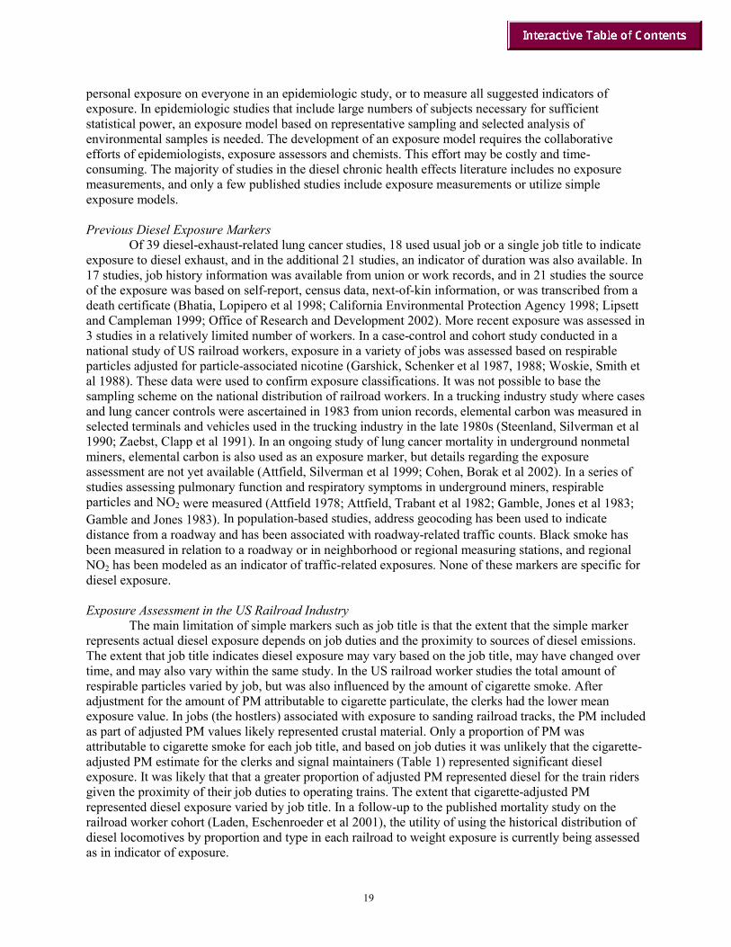
19

personal exposure on everyone in an epidemiologic study, or to measure all suggested indicators of exposure. In epidemiologic studies that include large numbers of subjects necessary for sufficient statistical power, an exposure model based on representative sampling and selected analysis of environmental samples is needed. The development of an exposure model requires the collaborative efforts of epidemiologists, exposure assessors and chemists. This effort may be costly and time-consuming. The majority of studies in the diesel chronic health effects literature includes no exposure measurements, and only a few published studies include exposure measurements or utilize simple exposure models. Previous Diesel Exposure Markers

Of 39 diesel-exhaust-related lung cancer studies, 18 used usual job or a single job title to indicate exposure to diesel exhaust, and in the additional 21 studies, an indicator of duration was also available. In 17 studies, job history information was available from union or work records, and in 21 studies the source of the exposure was based on self-report, census data, next-of-kin information, or was transcribed from a death certificate (Bhatia, Lopipero et al 1998; California Environmental Protection Agency 1998; Lipsett and Campleman 1999; Office of Research and Development 2002). More recent exposure was assessed in 3 studies in a relatively limited number of workers. In a case-control and cohort study conducted in a national study of US railroad workers, exposure in a variety of jobs was assessed based on respirable particles adjusted for particle-associated nicotine (Garshick, Schenker et al 1987, 1988; Woskie, Smith et al 1988). These data were used to confirm exposure classifications. It was not possible to base the sampling scheme on the national distribution of railroad workers. In a trucking industry study where cases and lung cancer controls were ascertained in 1983 from union records, elemental carbon was measured in selected terminals and vehicles used in the trucking industry in the late 1980s (Steenland, Silverman et al 1990; Zaebst, Clapp et al 1991). In an ongoing study of lung cancer mortality in underground nonmetal miners, elemental carbon is also used as an exposure marker, but details regarding the exposure assessment are not yet available (Attfield, Silverman et al 1999; Cohen, Borak et al 2002). In a series of studies assessing pulmonary function and respiratory symptoms in underground miners, respirable particles and NO2 were measured (Attfield 1978; Attfield, Trabant et al 1982; Gamble, Jones et al 1983; Gamble and Jones 1983). In population-based studies, address geocoding has been used to indicate distance from a roadway and has been associated with roadway-related traffic counts. Black smoke has been measured in relation to a roadway or in neighborhood or regional measuring stations, and regional NO2 has been modeled as an indicator of traffic-related exposures. None of these markers are specific for diesel exposure. Exposure Assessment in the US Railroad Industry

The main limitation of simple markers such as job title is that the extent that the simple marker represents actual diesel exposure depends on job duties and the proximity to sources of diesel emissions. The extent that job title indicates diesel exposure may vary based on the job title, may have changed over time, and may also vary within the same study. In the US railroad worker studies the total amount of respirable particles varied by job, but was also influenced by the amount of cigarette smoke. After adjustment for the amount of PM attributable to cigarette particulate, the clerks had the lower mean exposure value. In jobs (the hostlers) associated with exposure to sanding railroad tracks, the PM included as part of adjusted PM values likely represented crustal material. Only a proportion of PM was attributable to cigarette smoke for each job title, and based on job duties it was unlikely that the cigarette-adjusted PM estimate for the clerks and signal maintainers (Table 1) represented significant diesel exposure. It was likely that that a greater proportion of adjusted PM represented diesel for the train riders given the proximity of their job duties to operating trains. The extent that cigarette-adjusted PM represented diesel exposure varied by job title. In a follow-up to the published mortality study on the railroad worker cohort (Laden, Eschenroeder et al 2001), the utility of using the historical distribution of diesel locomotives by proportion and type in each railroad to weight exposure is currently being assessed as in indicator of exposure.

20

US Trucking Industry: Feasibility Assessment

A more comprehensive exposure database is being developed for a study of particle exposure and lung cancer and other chronic health outcomes in the US trucking industry. The assembly of this database will permit the development of a more complex exposure model in contrast to prior chronic health studies. The Trucking Industry Particle Study is funded by the National Cancer Institute and designed to assess lung cancer mortality in a cohort of 62,250 US trucking company workers. Current exposure to PM will be assessed by conducting representative terminal-based sampling throughout the United States. There are four main workplace exposure scenarios in the trucking industry (Figure 1). These scenarios include exposure in the cab of a pick-up and delivery truck (traveling on local roads), in a long haul tractor-trailer (traveling on intercity highways), on the terminal loading dock, and in the terminal shop. A main source of particle exposure is expected to be from diesel exhaust, but this will vary by job title and terminal. In the dock area there are emissions from idling trucks. In the past there were emissions from diesel forklifts, but currently only propane forklifts are used. In the shop areas workers do refueling and repairs, change tires, and change oil. There are emissions coming from the terminal yard, and upwind from the terminal (representing off-site sources of emissions), likely influenced by the extent of local traffic. Exposure in the cabs of local pick-up and delivery trucks will be influenced by local traffic mix.

In a feasibility study (Garshick, Smith et al 2002) conducted as part of the Health Effects Institute Diesel Feasibility Project, exposure was assessed in two large urban truck terminals in Atlanta and four small rural terminals in New England in 1999 over several days. Personal and area work-shift measurements of elemental carbon (EC), organic carbon (OC), and PM2.5 were obtained. High-volume particulate (16.7 LPM) samples were collected on the urban terminal loading dock over twelve hours. The purpose of the collection of samples by high-flow pumps rather than lower-flow personal pumps was to collect sufficient particle-bound organic material to permit the assessment of molecular tracers of exhaust emissions, as developed by Glenn Cass (Cass and Gray 1995) and James Schauer and colleagues (Schauer, Rogge et al 1996; Schauer, Kleeman et al 1998, 1999). Although EC was the main marker of exposure to sources of combustion, molecular markers identified in the particle-associated organics can be used to estimate the source of EC.

To assess the real-time contribution to PM measured on the loading dock from PM infiltrating from off-site, simultaneous recordings of PM2.5 were obtained using a Dust Trak, a technology based on light-scattering methodology (Figure 2). The PM peaks measured on the loading dock were superimposable on the baseline PM level obtained upwind. These tracings indicate that the local PM levels are greatly influenced by conditions surrounding the loading dock as well as local dock activities. This is also illustrated in the EC measurements. On the loading dock in the larger and smaller terminals, approximately half the EC was coming from off-site (Table 2). Therefore work at large urban terminals would indicate both high background and high occupational exposures, and work at small rural terminals would indicate low background and low occupational exposures. EC exposure varied also by job, with the higher EC values in the dockworkers and pick-up and delivery drivers (Table 3). These results indicate that variation in EC exposure on the loading docks in the US trucking industry will be best described by a model that considers terminal size (as a marker of the number of diesel vehicles) and urban or rural location as an indicator of conditions outside the terminal area. Other factors may also be important, such as truck year and model on the loading dock. For exposure in the cab of a truck, design features of the cab may also be important. However, the extent that a truck driver receives exposure from his/her own truck compared to a general mix reflecting vehicular traffic is unknown. EC As an Exposure Marker

EC is not unique to diesel, and a variety of combustion sources contribute, including wood smoke, spark engine emissions, coal emissions, and fuel oil combustion (Schauer, Kleeman et al 1998). Since the mechanism of chronic diseases possibly attributable to diesel exhaust is unknown, EC may be poorly correlated with actual disease agents, and depending on the emission source mix, EC may also be poorly correlated with diesel emissions. The measurement of EC alone would test the hypothesis that

21

combustion sources resulting in EC result in an adverse health effect. The emission contribution mix will vary based on work location, the time of day, and the operating characteristics of the engines. However, in a study that assesses chronic health outcomes such as lung cancer, the goal is to average across all sources of variation and estimate the relative contribution of each emission source to health risk. In the trucking industry pilot study, the composited area sample from loading docks indicated that idling diesel trucks were the main source. Cohort Selection Issues

Exposure measurements made without consideration of the epidemiologic database usually cannot be adequately linked to the assessment of health effects. Linkage between exposure markers and an epidemiologic database requires knowledge of current and historical exposure scenarios and factors influencing exposure. In previous efforts to develop an exposure model in the trucking industry (Steenland, Deddens et al 1998), efforts to link EC to job title were based on heavy-duty truck vehicle miles, engine emission factors, and an estimate of exhaust system leaks into cabs. It was not possible to adequately link the assumptions made about these determinants of exposure to the epidemiologic database or to validate the method of extrapolation. The only variables available in the epidemiologic database to link the proposed exposure model to each subject’s personal exposure were job title and years of work but there was no direct linkage to diesel truck use.

In contrast, much is known about the work history of subjects included in the Trucking Industry Particle Study cohort. The epidemiologic database for the Trucking Industry Particle Study includes nearly all job titles and work locations, company diesel vehicle mix, and dates of diesel vehicle use. Much is known about diesel vehicle use. Supplementary company data will permit the linkage of an exposure model and epidemiologic database based on terminal size and location, truck fleets, vehicle age, and possibly other factors (i.e., cab type, fuel type) to describe variation in exposure. Historical exposure estimation will be based on a matrix defined by job, terminal size and location, calendar interval, vehicle features, and other important characteristics. This will be less precise than current measurements, but will define semiquantitative job-location categories and ranking of exposures. Summary

The ideal marker of diesel exhaust exposure would be a single marker that would be inexpensive, easy to measure, and clearly linked to the source of diesel emissions. However, the reality is that diesel exhaust is a complex mixture, and in many real-life scenarios it may not be the only important source of exposure to the individual particles and gases that constitute diesel exhaust. In addition, the mechanism of health effects and specific causal agents are uncertain. The best diesel exposure marker is likely to be more complex and involve the measurements of molecular organic tracers and elemental carbon. The nature of the exposure assessment and marker chosen may also depend on mechanism of health effect postulated, and may include measurement of exhaust gases (such as ozone and NO2) in the setting of nonmalignant respiratory diseases.

Although current literature identifies diesel exhaust as a health hazard, insight into a dose-response relationship is limited by factors related to both cohort selection and exposure assessment. The development of an exposure model in the existing diesel exhaust epidemiologic literature is hindered by a lack of exposure measurements upon which an exposure model can be developed, uncertainty regarding the best measurement or marker(s) indicative of exposure, and uncertainty regarding historical exposures. Until recently, there has been little effort in understanding determinants of current exposures experienced by subjects driving through traffic or in other exposure scenarios typical of general population exposures. Once factors influencing current exposure (using exposure models proposed for the Trucking Industry Particle Study) have been assessed, it will be possible to address the development of historical exposure models for the trucking industry cohort. At the present time there is little information regarding how changes and differences in engine design, fuel type, and operating conditions influenced various markers of diesel exhaust exposure, or how proposed changes will alter the on-road profile of exposure. It is

22

suggested that research in this area be done to assess how changes in engine technology and operations affect markers of diesel exposure used in epidemiologic studies. References Attfield, M. (1978). The effect of exposure to silica and diesel exhaust in underground metal and

nonmetal miners. Industrial hygiene for mining and tunneling:proceedings of a topical symposium, Denver, CO, The American Conference of Governmental Industrial Hygienists, Inc.

Attfield, M., D. Silverman, et al. (1999). Lung cancer and diesel exhaust among non-metal miners in the United States. Paper presented at the HEI Diesel Workshop-Building a Research Strategy to Improve Risk Assessment. Stone Mountain, GA.

Attfield, M. D., G. D. Trabant, et al. (1982). “Exposure to diesel fumes and dust at six potash mines.” Ann Occup Hyg 26(1-4): 817-31.

Ballester, F., M. Saez, et al. (2002). “The EMECAM project: a multicentre study on air pollution and mortality in Spain: combined results for particulates and for sulfur dioxide.” Occup Environ Med 59(5): 300-8.

Bhatia, R., P. Lopipero, et al. (1998). “Diesel exhaust exposure and lung cancer.” Epidemiology 9(1): 84-91.

Boffetta, P. and D. T. Silverman (2001). “A meta-analysis of bladder cancer and diesel exhaust exposure.” Epidemiology 12(1): 125-30.

Brunekreef, B. and G. Hoek (2000). “Beyond the body count: air pollution and death.” Am J Epidemiol 151(5): 449-51.

Brunekreef, B., N. A. Janssen, et al. (1997). “Air pollution from truck traffic and lung function in children living near motorways.” Epidemiology 8(3): 298-303.

California Environmental Protection Agency (1998). Health Risk Assessment for Diesel Exhaust: Proposed Identification of Diesel Exhaust As a Toxic Air Contaminant. Sacramento, CA, Office of Environmental Health Hazard Assessment, Air Resources Board.

Cass, G. R. and H. A. Gray (1995). “Regional emissions and atmospheric concentrations of diesel engine particulate matter: Los Angeles as a case study. In: Health Effects Institute, Diesel exhaust: a critical analysis of emissions, exposure, and health effects. A special report of the Institute's Diesel Working Group.”.

Cohen, H. J., J. Borak, et al. (2002). “Exposure of miners to diesel exhaust particulates in underground nonmetal mines.” AIHA Journal 63: 651-658.

Diaz-Sanchez, D. (1997). “The role of diesel exhaust particles and their associated polyaromatic hydrocarbons in the induction of allergic airway disease.” Allergy 52(38): 52-6; discussion 57-8.

Diesel Epidemiology Working Group (2002). Research Directions to Improve Estimates of Human Exposure and Risk from Diesel Exhaust. Boston, MA, Health Effects Institute.

Dockery, D. W., A. C. d. Pope, et al. (1993). “An association between air pollution and mortality in six U.S. cities.” N Engl J Med 329(24): 1753-9.

Gamble, J., W. Jones, et al. (1983). “An epidemiological study of salt miners in diesel and nondiesel mines.” Am J Ind Med 4(3): 435-58.

Gamble, J. F. and W. G. Jones (1983). “Respiratory effects of diesel exhaust in salt miners.” Am Rev Respir Dis 128(3): 389-94.

Garshick, E., M. B. Schenker, et al. (1987). “A case-control study of lung cancer and diesel exhaust exposure in railroad workers.” Am Rev Respir Dis 135(6): 1242-8.

Garshick, E., M. B. Schenker, et al. (1988). “A retrospective cohort study of lung cancer and diesel exhaust exposure in railroad workers.” Am Rev Respir Dis 137(4): 820-5.

Garshick, E., T. J. Smith, et al. (2002). Quantitative Assessment of Lung Cancer Risk from Diesel Exhaust Exposure in the US Trucking Industry: A Feasibility Study. Research Directions to Improve Estimates of Human Exposure and Risk from Diesel Exhaust. Diesel Epidemiology Working Group. Boston, MA, Health Effects Institute.

23

HEI (1995). Diesel exhaust: A critical analysis of emissions, exposure, and health effects. Cambridge, MA, Health Effects Institute: 294.

Hoek, G., B. Brunekreef, et al. (2002). “Association between mortality and indicators of traffic-related air pollution in the Netherlands: a cohort study.” Lancet 360(9341): 1203-9.

Laden, F., A. Eschenroeder, et al. (2001). “Historical estimation of diesel exhaust exposure in a cohort study of railroad workers and lung cancer (abstract).” Am J Respir Crit Care Med 163: A717.

Le Tertre, A., S. Medina, et al. (2002). “Short-term effects of particulate air pollution on cardiovascular diseases in eight European cities.” J Epidemiol Community Health 56(10): 773-9.

Lipsett, M. and S. Campleman (1999). “Occupational exposure to diesel exhaust and lung cancer: a meta- analysis.” Am J Public Health 89(7): 1009-17.

Mar, T. F., G. A. Norris, et al. (2000). “Associations between air pollution and mortality in Phoenix, 1995-1997.” Environ Health Perspect 108(4): 347-53.

Nel, A. E., D. Diaz-Sanchez, et al. (1998). “Enhancement of allergic inflammation by the interaction between diesel exhaust particles and the immune system.” J Allergy Clin Immunol 102(4 Pt 1): 539-54.

Office of Research and Development (2002). Health Assessment Document for Diesel Engine Exhaust. Washington, DC, National Center for Environmental Assessment, U.S. Environmental Protection Agency.

Schauer, J. J., M. J. Kleeman, et al. (1998). Characterization and control of organic compounds emitted from air pollution sources. Final Report Contract No. 93-329. Sacramento, CA, California Air Resources Board.

Schauer, J. J., M. J. Kleeman, et al. (1999). Characterization and Control of Organic Compounds Emitted from Air Pollution Sources. PB99-118937. Springfield, VA, California Air Resources Board.

Schauer, J. J., W. Rogge, et al. (1996). “Source apportionment of airborne particulate matter using organic compounds as tracers.” Atmos Environ 30: 3837-3855.

Schwartz, J. (1994). “Air pollution and hospital admissions for the elderly in Birmingham, Alabama.” Am J Epidemiol 139(6): 589-98.

Schwartz, J., F. Ballester, et al. (2001). “The concentration-response relation between air pollution and daily deaths.” Environ Health Perspect 109(10): 1001-6.

Schwartz, J., D. W. Dockery, et al. (1996). “Is daily mortality associated specifically with fine particles?” J Air Waste Manag Assoc 46(10): 927-39.

Schwartz, J. and R. Morris (1995). “Air pollution and hospital admissions for cardiovascular disease in Detroit, Michigan.” Am J Epidemiol 142(1): 23-35.

Schwartz, J. and L. M. Neas (2000). “Fine particles are more strongly associated than coarse particles with acute respiratory health effects in schoolchildren.” Epidemiology 11(1): 6-10.

Steenland, K., J. Deddens, et al. (1998). “Diesel exhaust and lung cancer in the trucking industry: exposure-response analyses and risk assessment.” Am J Ind Med 34(3): 220-8.

Steenland, N. K., D. T. Silverman, et al. (1990). “Case-control study of lung cancer and truck driving in the Teamsters Union.” Am J Pub Health 80(6): 670-674.

van Vliet, P., M. Knape, et al. (1997). “Motor vehicle exhaust and chronic respiratory symptoms in children living near freeways.” Environ Res 74(2): 122-32.

Woskie, S. R., T. J. Smith, et al. (1988). “Estimation of the diesel exhaust exposures of railroad workers: I. Current exposures.” Am J Ind Med 13(3): 381-94.

Zaebst, D. D., D. E. Clapp, et al. (1991). “Quantitative determination of trucking industry workers' exposures to diesel exhaust particles.” Am Ind Hyg Assoc J 52(12): 529-41.

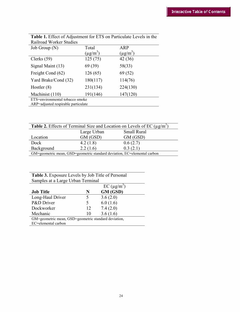
24

Table 1. Effect of Adjustment for ETS on Particulate Levels in the Railroad Worker Studies Job Group (N) Total

(µg/m3) ARP (µg/m3)

Clerks (59) 125 (75) 42 (36) Signal Maint (13) 69 (39) 58(33) Freight Cond (62) 126 (65) 69 (52) Yard Brake/Cond (32) 180(117) 114(76) Hostler (8) 231(134) 224(130) Machinist (110) 191(146) 147(120) ETS=environmental tobacco smoke ARP=adjusted respirable particulate

Table 2. Effects of Terminal Size and Location on Levels of EC (µg/m3) Large Urban Small Rural Location GM (GSD) GM (GSD) Dock 4.2 (1.8) 0.6 (2.7) Background 2.2 (1.6) 0.3 (2.1) GM=geometric mean, GSD=geometric standard deviation, EC=elemental carbon

Table 3. Exposure Levels by Job Title of Personal Samples at a Large Urban Terminal EC (µg/m3) Job Title N GM (GSD) Long-Haul Driver 5 3.6 (2.0) P&D Driver 5 6.0 (1.6) Dockworker 12 7.4 (2.0) Mechanic 10 3.6 (1.6) GM=geometric mean, GSD=geometric standard deviation, EC=elemental carbon

25

Figure 1. Trucking Industry Particle Study potential emission sources.

Figure 2. Variation in real-time PM2.5 in dock area and upwind of an urban Atlanta terminal.

*CAB

Pollution

Traffic Emissions In-Terminal Emissions In-Shop EmissionsYard Emissions

TERMINAL SHOP

Dock area

*Cab== Long haul (highway) or Pick-up and delivery truck (city)

0

0.02

0.04

0.06

0.08

0.1

0.12

0.14

9:41 AM 10:31 AM 11:21 AM 12:11 PM 1:01 PM 1:51 PM 2:41 PM 3:31 PM 4:21 PM

Time

PM2.

5 (u

g/m

^3)

Dock

Yard Background Level

Contribution of Background PM to occupational exposure

27

Issues in Exposure Assessment in Epidemiologic Studies

of Acute Effects of Diesel Exhaust

Patrick L. Kinney Columbia University, New York, New York

This paper discusses exposure assessment in epidemiology studies of acute air pollution effects, with an emphasis on strengths and limitations of study designs with respect to investigating the specific health impacts of diesel exhaust as distinct from the effects of pollutants emitted by nondiesel sources. To date, acute epidemiology studies have yielded some hints of health impacts from motor vehicle exhaust particles, but have not implicated diesel particulate matter (DPM) specifically. I argue that standard acute study designs, e.g., ecologic designs in which central-site PM monitoring data are correlated over time with daily mortality or morbidity, are unlikely to provide very useful information on DPM-specific effects, whether or not a specific signature of airborne DPM becomes available for use in such studies. This pessimism reflects the fundamental limitations of the standard design for addressing this question, including the high degree of natural temporal correlation between all particle components due to their joint dependence on meteorology, and the relatively greater magnitude of spatial variations in ambient DPM as compared with sulfate and nitrate aerosols, leading to increased exposure misclassification when employing central-site DPM samples. In contrast, innovative acute study designs that exploit uniquely occurring DPM exposure patterns, such as diesel-only roadways or diurnal patterns in traffic, hold more promise for documenting specific health impacts of DPM. Here I define acute studies as those in which exposure and associated health impacts are assessed over short time intervals (e.g., a few minutes to a few days), and short-term variations in exposure are thought to drive health responses. This definition excludes studies that investigate respiratory effects of spatial variations in exposure, even if the health outcomes under study include “acute” respiratory symptoms. Recent Insights from Epidemiology Studies

Several studies using the ecologic time series design have hinted at a motor vehicle signal in the acute effects of central-site air pollution on daily mortality or hospital admission counts in urban areas (Janssen et al., 2002; Burnett et al., 1997a, 1997b, 1998, 2000; Fairley, 1999; Gwynn et al., 2000; Lipfert et al., 2000; Mar et al., 2000; Hoek et al., 2000; Goldberg et al., 2000; Anderson et al., 2001; Laden et al., 2000; Tsai et al., 2000; Wichmann et al., 2000). Most of these studies observed significant health effects for pollutants usually viewed as being dominated by motor vehicle emissions in urban areas, including black carbon (elemental carbon, black smoke, or coefficient of haze), CO, NO2, ultrafine particles, and/or Pb, as well as other pollutants such as PM10. In some cases motor vehicle pollutant associations were more robust than were those for gravimetric PM metrics (e.g., PM10); in other cases they were not. The general conclusion that emerges from this literature is that pollutants derived from motor vehicles often play an important role in acute mortality and morbidity effects of air pollution.

Most of the studies mentioned above based their conclusions on multiple regression analyses on alternative pollutants, a widely understood and accepted approach for investigating effects of various factors on an outcome. However, in several cases, other approaches were used to more explicitly address source-specific effects. In an analysis of regression coefficients of hospital admissions on PM10 from 14 US cities, Janssen et al. 2002 reported larger coefficients in those cities where motor vehicles were thought to contribute larger shares to the total PM loading of the atmosphere. Figure 1 displays these results. Several groups reported motor vehicle health impacts from studies examining mortality impacts of source-related pollutant mixtures, i.e., linear combinations of multiple air pollutants in which the relative weights, derived from factor analysis, suggest the influence of particular sources (Laden et al., 2000; Mar

28

et al., 2000; Tsai et al., 2000). Depending on the mix of pollutants available and the study size, factor analysis often can distinguish several apparent source signals, including motor vehicles (related to elemental Pb, black carbon, CO, and/or NO2), fuel oil combustion (elemental V), coal combustion (elemental Se), and soil particles (Si or other crustal elements).

Although many of the ecologic time series studies noted above suggest the importance of motor vehicle emissions, it has not been possible from these results to uniquely attribute PM effects to motor vehicles or any other particular source class. Nor has it even been possible to quantitatively rank the importance of different PM sources. This has been the case for broadly defined source classes, such as motor vehicles, and certainly would be the case for more specific subclasses, such as diesel vs. spark ignition vehicles, assuming that specific metrics existed. This is due to inherent limitations in the ecologic time series study design, including the aggregation of health and exposure variables into 24-hour time intervals, the high temporal correlations that usually exist among pollutants when measured at the daily level, making statistical separation of pollutant effects nearly impossible, and varying levels of exposure misclassification when using central-site data. It is important to note that merely adding new exposure metrics in this setting will not overcome these limitations and is unlikely to yield major insights on source-specific effects. So, is there value in colocating an extensive array of PM size and compositional monitoring technology at central sites where time series epidemiology studies can be carried out ("super-duper" sites)? I consider such studies valuable in that the monitoring data are inherently important for urban aerosol characterization, and companion ecologic time series studies would be inexpensive and easy to carry out — and might generate hypotheses that are worth following up in other designs. However, we should not expect definitive results regarding component- or source-specific health impacts from these studies. Exposure Challenges The central challenge for any epidemiology study seeking to examine diesel-specific health impacts is the lack of a distinctive aerosol signature for diesel emissions. All available evidence points to the qualitative similarities between emissions from diesel and spark ignition engines. For some components, such as elemental carbon, diesel vehicles tend to emit greater quantities per mile. But since spark ignition vehicles often far outnumber diesel vehicles, these differences are obscured in the ambient aerosol mix.

A related point is that, given the qualitative similarity of emissions, it is not clear that one would expect the health effects resulting from exposure to be different for the two engine types. From a scientific perspective, it may be more productive to treat diesel and spark ignition vehicles as two different sources of the same mix of potentially toxic pollutants. This thinking would lead to studies targeting the further characterization of the health impacts of motor vehicle pollutants, and policy interventions to reduce population exposures to motor vehicle pollutants. In some settings diesel vehicles might be the dominant source; in many others spark ignition vehicles would dominate. While acknowledging this challenge, it is worth noting that elemental carbon has historically been a useful indicator of diesel emission impacts in urban areas. It has many desirable attributes of a useful indicator: diesel vehicles are often the dominant source type in urban areas, elemental carbon is relatively stable in the atmosphere over time; it is inexpensive and easy to measure over short and long time intervals; and it has been shown empirically to correlate with diesel vehicle counts (Kinney et al., 2000; Lena et al., 2002). Atmospheric stability is a particularly valuable characteristic of a source indicator; reactions that occur between the source and the monitor diminish the value of a source indicator. Any new candidate diesel indicator should be assessed with respect to these attributes. For the foreseeable future, EC will remain a useful indicator of DPM in epidemiology studies. Because acute epidemiology studies usually exploit naturally occurring temporal variations in air pollution concentrations to drive population exposure differences, such studies are most suited for pollutants with pronounced temporal variations. Further, since population exposures are usually represented by a very limited number of central-site monitors, acute epidemiology works best for

29

pollutants that have minimal spatial variations over the scale of an urban area, so that the temporal fluctuations measured at the central site reflect fluctuations in population exposures. Recent studies have shown that motor vehicle pollutants possess considerably more spatial than temporal variability in urban areas. For example, EC concentrations in New York City, which in the summer are driven largely by diesel emissions, possessed considerably more spatial than temporal variations within the Hunts Point neighborhood of the South Bronx (Lena et al., 2002). PM2.5 exhibited the reverse, with temporal variations being dominant. The dampened temporal variability for EC probably reflects the nearly constant day-to-day average emissions from local traffic in NYC, whereas the more pronounced spatial variability reflects the marked geographic variations in traffic density. It should also be noted that Lena and colleagues only monitored concentrations on weekdays, thus potentially missing weekend- vs.-weekday temporal variations. These results suggest that typical acute study designs (e.g., daily time series) are less well suited to the study of DPM than of PM2.5, since temporal variations are weak and central-site concentrations are less representative of population exposures. Exposure Opportunities

The above discussion argues against relying on standard acute epidemiology study designs to gain insights into the health impacts of motor vehicle pollutants including DPM because of the inherent limitations of central-site data in representing population exposures. Indeed, given the substantial spatial character of traffic-related emissions and exposures, it has been and will continue to be more productive to examine health effects in the context of spatial study designs, such as those assessing health status among groups living near vs. far from roadways. However, there are opportunities for assessing acute effects of DPM using creative study designs that capture or create short-term variations in exposure.

Most acute studies to date have relied on naturally occurring daily variations in ambient concentrations of pollutants within a single location to drive the outcome. I’ve argued that this is misguided when interest focuses on motor vehicle pollutants. An alternative is to capture the very short-term variations in personal exposures that occur for individuals who move through a spatial distribution of ambient concentrations. Motorists, cyclists, or runners who move in and out of areas dominated by diesel vehicle emissions would be examples. Bus-only vs. car-only tunnels could be studied. Zhang and colleagues recently initiated a study in which volunteers perform programmed 2-hour walks in London, either along a road dominated by diesel vehicles or in a park, and then receive detailed health assessments in a clinic (Jim Zhang, personal communication). Innovative studies like this hold considerable promise to advance our understanding of the acute effects of DPM.

Another approach would be to take advantage of temporal variations in vehicle mix that may occur over hours within days or between weekdays and weekends. Morning rush hours in cities may be dominated by auto traffic whereas late morning traffic may be dominated by diesel delivery vehicles. Trucks are generally more active on weekdays than on weekends. Some areas have restrictions on auto traffic that vary over the day. Numerous opportunities probably exist for innovative study designs; identifying and capitalizing on them will require a high degree of communication between transportation departments and epidemiologists. Looking to the Future An important conclusion of this paper is that acute epidemiology addressing DPM or motor vehicle pollution in general will be challenging, regardless of the airborne signature that is monitored. The patterns of exposure to motor vehicle pollution that have been observed to date indicate that spatial epidemiologic designs generally will be more informative than acute studies. However, innovative acute studies that capture well-characterized temporal variations in personal exposure are valuable to pursue.

New study designs that target individual exposures and health effects will benefit from lightweight, portable, and quiet personal monitors that can capture the particle components of interest (e.g., EC, certain organics, ultrafine particles) over appropriate time scales (1- to 2-hour resolution).

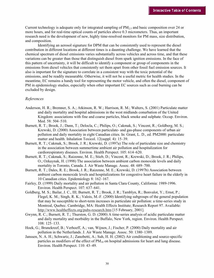
30

Current technology is adequate only for integrated sampling of PM2.5 and basic composition over 24 or more hours, and for real-time optical counts of particles above 0.3 micrometers. Thus, an important research need is the development of new, highly time-resolved monitors for PM mass, size distribution, and composition. Identifying an aerosol signature for DPM that can be consistently used to represent the diesel contribution in different locations at different times is a daunting challenge. We have learned that the chemical spectrum of diesel emissions varies substantially across vehicles and across time, and that these variations can be greater than those that distinguish diesel from spark ignition emissions. In the face of this pattern of uncertainty, it will be difficult to identify a component or group of components in the emissions from diesel vehicles that consistently set them apart from other fossil fuel emission sources. It also is important for the signature to correlate in a consistent way with the toxic potential of the emissions, and be readily measurable. Otherwise, it will not be a useful metric for health studies. In the meantime, EC remains a handy tool for representing the motor vehicle, and often the diesel, component of PM in epidemiology studies, especially when other important EC sources such as coal burning can be excluded by design. References Anderson, H. R.; Bremner, S. A.; Atkinson, R. W.; Harrison, R. M.; Walters, S. (2001) Particulate matter

and daily mortality and hospital admissions in the west midlands conurbation of the United Kingdom: associations with fine and coarse particles, black smoke and sulphate. Occup. Environ. Med. 58: 504–510.

Burnett, R. T.; Brook, J.; Dann, T.; Delocla, C.; Philips, O.; Cakmak, S.; Vincent, R.; Goldberg, M. S.; Krewski, D. (2000) Association between particulate- and gas-phase components of urban air pollution and daily mortality in eight Canadian cities. In: Grant, L. D., ed. PM2000: particulate matter and health. Inhalation Toxicol. 12(suppl. 4): 15–39.

Burnett, R. T.; Cakmak, S.; Brook, J. R.; Krewski, D. (1997a) The role of particulate size and chemistry in the association between summertime ambient air pollution and hospitalization for cardiorespiratory diseases. Environ. Health Perspect. 105: 614–620.

Burnett, R. T.; Cakmak, S.; Raizenne, M. E.; Stieb, D.; Vincent, R.; Krewski, D.; Brook, J. R.; Philips, O.; Ozkaynak, H. (1998) The association between ambient carbon monoxide levels and daily mortality in Toronto, Canada. J. Air Waste Manage. Assoc. 48: 689–700.

Burnett, R. T.; Dales, R. E.; Brook, J. R.; Raizenne, M. E.; Krewski, D. (1997b) Association between ambient carbon monoxide levels and hospitalizations for congestive heart failure in the elderly in 10 Canadian cities. Epidemiology 8: 162–167.

Fairley, D. (1999) Daily mortality and air pollution in Santa Clara County, California: 1989-1996. Environ. Health Perspect. 107: 637–641.

Goldberg, M. S.; Bailar, J. C., III; Burnett, R. T.; Brook, J. R.; Tamblyn, R.; Bonvalot, Y.; Ernst, P.; Flegel, K. M.; Singh, R. K.; Valois, M.-F. (2000) Identifying subgroups of the general population that may be susceptible to short-term increases in particulate air pollution: a time-series study in Montreal, Quebec. Cambridge, MA: Health Effects Institute; Research Report 97. Available: http://www.healtheffects.org/pubs-research.htm [15 February, 2001].

Gwynn, R. C.; Burnett, R. T.; Thurston, G. D. (2000) A time-series analysis of acidic particulate matter and daily mortality and morbidity in the Buffalo, New York, region. Environ. Health Perspect. 108: 125–133.

Hoek, G.; Brunekreef, B.; Verhoeff, A.; van, Wijnen, J.; Fischer, P. (2000) Daily mortality and air pollution in the Netherlands. J. Air Waste Manage. Assoc. 50: 1380–1389.

Janssen, N. A. H.; Schwartz, J.; Zanobetti, A.; Suh, H. H. (2002) Air conditioning and source-specific particles as modifiers of the effect of PM10 on hospital admissions for heart and lung disease. Environ. Health Perspect. 110: 43–49.

31

Kinney, P.L., Aggarwal, M., Northridge, M.E., Janssen, N.A.H., and Shepard, P. (2000) Airborne concentrations of PM2.5 and diesel exhaust particles on Harlem sidewalks: a community-based pilot study. Environ. Health Perspect. 108:213–218.

Laden, F.; Neas, L. M.; Dockery, D. W.; Schwartz, J. (2000) Association of fine particulate matter from different sources with daily mortality in six U.S. cities. Environ. Health Perspect. 108: 941-947.

Lena, T.S., Ochieng, V., Carter, M., Holguín-Veras, J., and Kinney, P.L. (2002) Elemental carbon and PM2.5 levels in an urban community heavily impacted by truck traffic. Environ. Health Perspect. 110:1009–1015.

Lipfert, F. W.; Morris, S. C.; Wyzga, R. E. (2000) Daily mortality in the Philadelphia metropolitan area and size-classified particulate matter. J. Air Waste Manage. Assoc.: 1501–1513.

Mar, T. F.; Norris, G. A.; Koenig, J. Q.; Larson, T. V. (2000) Associations between air pollution and mortality in Phoenix, 1995–1997. Environ. Health Perspect. 108: 347–353.

Tsai, F. C.; Apte, M. G.; Daisey, J. M. (2000) An exploratory analysis of the relationship between mortality and the chemical composition of airborne particulate matter. Inhalation Toxicol. 12(suppl.): 121–135.

Wichmann, H.-E.; Spix, C.; Tuch, T.; Wolke, G.; Peters, A.; Heinrich, J.; Kreyling, W. G.; Heyder, J. (2000) Daily mortality and fine and ultrafine particles in Erfurt, Germany. Part I: role of particle number and particle mass. Cambridge, MA: Health Effects Institute; Research Report 98.

Figure 1.

Janssen et al., Environmental Health Perspectives, January 2002

Univariate relation between percentage of PM10 from highway vehicles and regression coefficients for cardiovascular diseases.

33

US EPA’s Health Assessment Document for Diesel Engine Exhaust

Charles Ris US Environmental Protection Agency. Washington DC

Introduction The US EPA’s Health Assessment Document for Diesel Engine Exhaust (May 2002, EPA/600/9-90/057F) represents its first comprehensive review of the potential health effects from ambient exposure to exhaust from diesel engines. The assessment was developed to provide information about the potential for diesel exhaust (DE) to pose environmental health hazards, information that would be useful in evaluating regulatory needs under provisions of the Clean Air Act. The assessment identifies and characterizes the potential human health hazards of DE (i.e, hazard assessment) and seeks to estimate the relationship between exposure and disease response for the key health effects (i.e., dose-response assessment). A full exposure assessment and risk characterization, the other two components of a complete risk assessment, are beyond the scope of this document. The EPA report has nine chapters and three appendices. Chapter 2 provides a characterization of diesel emissions, atmospheric transformation, and human exposures to provide a context for the hazard evaluation of DE. Other chapters provide reviews of relevant information for the evaluation of potential health hazards of DE, including dosimetry (Chapter 3), mutagenicity (Chapter 4), noncancer effects (Chapter 5), and carcinogenic effects (Chapter 7). Chapters 6 and 8 contain dose-response analyses to provide insight about the significance of the key noncancer and cancer hazards. Chapter 9 summarizes and characterizes the overall nature of the health hazard potential in the environment and the overall confidence and/or uncertainties associated with the conclusions. Composition of Diesel Exhaust DE is a complex mixture of hundreds of constituents in either a gas or particle form. Gaseous components of DE include carbon dioxide, oxygen, nitrogen, water vapor, carbon monoxide, nitrogen compounds, sulfur compounds, and numerous low molecular weight hydrocarbons. Among the gaseous hydrocarbon components of DE that are individually known to be of toxicologic relevance are the aldehydes (e.g., formaldehyde, acetaldehyde, acrolein), benzene, 1,3-butadiene, and polycyclic aromatic hydrocarbons (PAHs) and nitro-PAHs. The particles present in DE (i.e., diesel particulate matter [DPM]) are composed of a center core of elemental carbon and adsorbed organic compounds, as well as small amounts of sulfate, nitrate, metals, and other trace elements. DPM consists of fine particles (fine particles have a diameter <2.5 µm), including a subgroup with a large number of ultrafine particles (ultrafine particles have a diameter <0.1 µm). Collectively, these particles have a large surface area which makes them an excellent medium for adsorbing organics. Also, their small size makes them highly respirable and able to reach the deep lung. A number of potentially toxicologically relevant organic compounds are on the particles. The organics, in general, range from about 20% to 40% of the particle weight, though higher and lower percentages are also reported. Many of the organic compounds present on the particles and in the gases are individually known to have mutagenic and carcinogenic properties. For example, PAHs, nitro-PAHs, and oxidized PAH derivatives are present on the diesel particles, with the PAHs and their derivatives constituting about 1% or less of the DPM mass. DE emissions vary significantly in chemical composition and particle size between different engine types (heavy-duty, light-duty), engine operating conditions (idle, accelerate, decelerate), and fuel formulations (high/low sulfur fuel). Also, there are emission differences between on-road and nonroad engines simply because the nonroad engines to date are generally of older technology. The mass of particles and the organic components on the particles emitted from on-road diesel engines have been reduced over the years. Available data for on-road engines indicate that toxicologically relevant organic components of DE (e.g., PAHs, nitro-PAHs) emitted from older vehicle engines are still present in

34

emissions from newer engines, though relative amounts have decreased. There is currently insufficient information to characterize the changes in the composition of DE from nonroad diesel engines over time. Diesel Exhaust as a Component of Ambient Particulate Matter DE is emitted from on-road diesel engines (vehicle engines) or nonroad diesel engines (e.g., locomotives, marine vessels, heavy-duty equipment). Nationwide, data in 1998 indicated that DE as measured by DPM made up about 6% of the total ambient PM2.5 inventory (i.e., particles with aerodynamic diameter of 2.5 µm or less) and about 23% of the inventory, if natural and miscellaneous sources of PM2.5 were excluded. Estimates of the DPM percentage of the total inventory in urban centers are higher. For example, estimates range from 10% to 36% in some urban areas in California, Colorado, and Arizona. Available data also indicate that over the years there have been significant reductions in DPM emissions from the exhaust of on-road diesel engines, whereas limited data suggest that exhaust emissions from nonroad engines have increased. Atmospheric Transformation of Diesel Exhaust After emission from the tailpipe, DE undergoes dilution and chemical and physical transformations in the atmosphere, as well as dispersion and transport in the atmosphere. The atmospheric lifetime for some compounds present in DE ranges from hours to days. DPM is directly emitted from diesel-powered engines (primary particulate matter) and can be formed from the gaseous compounds emitted by diesel engines (secondary particulate matter). Limited information is available about the physical and chemical transformation of DE in the atmosphere. It is not clear what the overall toxicological consequences of DE’s transformations are because some compounds in the DE mixture are altered to more toxic forms while others are made less toxic. Exposure to Diesel Exhaust DPM mass (expressed as µg DPM/m3) has historically been used as a surrogate measure of exposure for whole DE. Although uncertainty exists as to whether DPM is the most appropriate parameter to correlate with human health effects, it is considered a reasonable choice until more definitive information about the mechanisms of toxicity or mode(s) of action of DE becomes available. In the ambient environment, human exposure to DE comes from both on-road and nonroad engine exhaust. A large percentage of the US population also is exposed to ambient PM2.5, of which DPM is typically a significant constituent. Although this EPA document does not provide an exposure assessment, DE exposure information is included to provide a context for the health effects information. Exposure estimates for the early to mid-1990s suggest that national annual average DE exposure from on-road engines alone ranged in many rural and urban areas between about 0.5 and 0.8 µg DPM/m3 of inhaled air. Exposures can be higher if a nonroad DE source adds to the exposure from on-road vehicles. For example, preliminary estimates show that, on a national average basis, accounting for nonroad DE emissions increases the on-road exposure twofold. For localized urban areas where people spend a large portion of their time outdoors, the exposures are higher and, for example, may range up to 4.0 µg DPM/m3 of inhaled air. Health Effects of Diesel Exhaust

Available evidence indicates that there are human health hazards associated with exposure to DE. The hazards include acute exposure-related symptoms, chronic exposure- related noncancer respiratory effects, and lung cancer. The health hazard conclusions are based on exhaust emissions from diesel engines built prior to the mid-1990s. With current engine use including some new and many more older engines (engines typically stay in service for a long time), the health hazard conclusions, in general, are applicable to engines currently in use. As new and cleaner diesel engines, together with different diesel fuels, replace a substantial number of existing engines, the general applicability of the health hazard conclusions will need to be re-evaluated. With new engine and fuel technology expected to produce significantly cleaner engine exhaust by 2007 (e.g., in response to new federal heavy-duty engine

35

regulations), significant reductions in public health hazards are expected for those engine uses affected by the regulations. Acute (Short-Term Exposure) Effects

Information is limited for characterizing the potential health effects associated with acute or short-term exposure. However, on the basis of available human and animal evidence, it is concluded that acute or short-term (e.g., episodic) exposure to DE can cause acute irritation (e.g., eye, throat, bronchial), neurophysiological symptoms (e.g., lightheadedness, nausea), and respiratory symptoms (cough, phlegm). There also is evidence for an immunologic effect—the exacerbation of allergenic responses to known allergens and asthma-like symptoms. The lack of adequate exposure-response information in the acute health effect studies precludes the development of recommendations about levels of exposure that would be presumed safe for these effects.

Chronic (Long-Term Exposure) Noncancer Respiratory Effects

Information from the available human studies is inadequate for a definitive evaluation of possible noncancer health effects from chronic exposure to DE. However, on the basis of extensive animal evidence, DE is judged to pose a chronic respiratory hazard to humans. Chronic-exposure, animal inhalation studies show a spectrum of dose-dependent inflammation and histopathological changes in the lung in several animal species including rats, mice, hamsters, and monkeys.

This assessment provides an estimate of inhalation exposure to DE (as measured by DPM), to which humans may be exposed throughout their lifetime without being likely to experience adverse noncancer respiratory effects. Known as the reference concentration (RfC), this expsoure level for DE of 5 µg/m3 of DPM was derived on the basis of dose-response data on inflammatory and histopathological changes in the lung from rat inhalation studies. In recognition of the presence of DPM in ambient PM2.5, it also is appropriate to consider the wealth of PM2.5 human health effects data. In this regard, the 1997 National Ambient Air Quality Standard for PM2.5 of 15 µg/m3 (annual average concentration) also would be expected to provide a measure of protection from DPM, reflecting the current approximate proportion of DPM to PM2.5. Chronic (Long-Term Exposure) Carcinogenic Effects

This EPA assessment concludes that DE is “likely to be carcinogenic to humans by inhalation” and that this hazard applies to environmental exposures. This conclusion is based on the totality of evidence from human, animal, and other supporting studies. There is considerable evidence demonstrating an association between DE exposure and increased lung cancer risk among workers in varied occupations where diesel engines historically have been used. The human evidence from occupational studies is considered strongly supportive of a finding that DE exposure is causally associated with lung cancer, though the evidence is less than that needed to definitively conclude that DE is carcinogenic to humans. There is some uncertainty about the degree to which confounders are having an influence on the observed cancer risk in the occupational studies, and there is uncertainty evolving from the lack of actual DE exposure data for the workers. In addition to the human evidence, there is supporting evidence for the carcinogenicity of DPM and associated DPM organic compound extracts in rats and mice exposed by noninhalation routes. Other supporting evidence includes the demonstrated mutagenic and chromosomal effects of DE and its organic constituents, and suggestive evidence for bioavailability of the DPM organics in humans and animals. Although high-exposure chronic rat inhalation studies show a significant lung cancer response, this is not thought predictive of a human hazard at lower environmental exposures. The rat response is considered to result from an overload of particles in the lung caused by the high exposure, and such an overload is not expected to occur in humans at environmental exposures. Although the available human evidence shows a lung cancer hazard to be present at occupational exposures that are generally higher than environmental levels, it is reasonable to presume that the hazard extends to environmental exposure levels. While the mode of action for DE-induced lung cancer that may

36

occur in humans is not completely understood, there is the potential for a nonthreshold mutagenic mode of action stemming from the organics in the DE mixture. A case for an environmental hazard also is shown by the simple observation that the estimated higher environmental exposure levels are close to, if not overlapping, the lower range of occupational exposures for which lung cancer increases are reported. These considerations taken together support the prudent public health choice of presuming a cancer hazard for DE at environmental levels of exposure. Overall, the evidence for a potential cancer hazard to humans resulting from chronic inhalation exposure to DE is persuasive, even though assumptions and uncertainties are involved. While the hazard evidence is persuasive, this does not lead to similar confidence in understanding the exposure/dose-response relationship. Given a carcinogenicity hazard, EPA typically performs a dose-response assessment of the human or animal data to develop a cancer unit risk estimate that can be used with exposure information to characterize the potential cancer disease impact on an exposed population. The DE exposure-response data for humans are considered too uncertain to derive a confident quantitative estimate of cancer unit risk, and with the chronic rat inhalation studies not being predictive for environmental levels of exposure, EPA has not developed a quantitative estimate of cancer unit risk. In the absence of a cancer unit risk, simple exploratory analyses were used to provide a perspective of the range of possible lung cancer risk from environmental exposure to DE. The analyses make use of reported lung cancer risk increases in occupational epidemiologic studies, and the differences between occupational and environmental exposures. The purpose of having a risk perspective is to illustrate and have a sense of the possible significance of the lung cancer hazard from environmental exposures. The risk perspective cannot be viewed as a definitive quantitative characterization of cancer risk, nor is it suitable for estimation of exposure-specific population risks. Sources of Uncertainty in the EPA Assessment

Even though the overall evidence for potential human health effects of DE is persuasive, many uncertainties exist because of the use of assumptions to bridge data and knowledge gaps about human exposures to DE and the general lack of understanding about underlying mechanisms by which DE causes observed toxicities in humans and animals. A notable uncertainty of this assessment is whether the health hazards identified from studies using emissions from older engines can be applied to present-day environmental emissions and related exposures, as some physical and chemical characteristics of the emissions from certain sources have changed over time. Available data are not sufficient to provide definitive answers to this question because changes in DE composition over time cannot be confidently quantified, and the relationship between the DE components and the mode(s) of action for DE toxicity is unclear. While recognizing the uncertainty, for this assessment, a judgment is made that prior-year toxicologic and epidemiologic findings can be applied to more current exposures, both of which use DPM mass in air as the measure of DE exposure. Other uncertainties include the assumptions that health effects observed at high doses may be applicable to low doses, and that toxicologic findings in laboratory animals generally are predictive of human responses. In the absence of a more complete understanding of how DE may cause adverse health effects in humans and laboratory animals, related assumptions (i.e., the presence of a biological threshold for chronic respiratory effects based on cumulative dosage and absence of a threshold for lung cancer stemming from subtle and irreversible effects) are considered reasonable and prudent. Although parts of this assessment, particularly the noncancer RfC estimate, have been derived with a generic consideration of sensitive subgroups within the population, the actual spectrum of the population that may have a greater susceptibility to DE is unknown and cannot be better characterized until more information is available regarding the adverse effects of DPM in humans. Increased susceptibility, for example, could result from above-average increases in DE deposition and retention in the respiratory system or intrinsic differences in respiratory system tissue sensitivity. There is no DE-specific information that provides direct insight to the question of differential human susceptibility. Given the nature of DE’s noncancer effects on the respiratory system, it would be reasonable, for example, to

37

consider possible vulnerable subgroups to include infants and children, the elderly, and individuals with preexisting health conditions, particularly respiratory conditions. In developing a perspective on the possible significance of the environmental cancer hazard of DE, this assessment uses information about the differences in the magnitude of DE exposures between occupational and environmental settings. Although an appreciation for differences in exposure is needed only at an order-of-magnitude level for this assessment, one should recognize that individual exposure is a function of both the variable concentrations in the environment and the related breathing and particle-retention patterns of the individual. Because of variations in these factors across the population, different subgroups could receive lower or higher exposure to DE than the groups mentioned in this assessment. Lastly, this assessment considers only potential heath effects from exposures to DE alone. Effects of DE exposure could be additive to or synergistic with concurrent exposures to many other air pollutants. However, in the absence of more definitive data demonstrating interactive effects (e.g., potentiation of allergenicity effects, potentiation of DPM toxicity by ambient ozone and oxides of nitrogen) from combined exposures to DE and other pollutants, it is not possible to address this issue. Further research is needed to improve knowledge of and data on DE exposures and potential human health effects, and thereby reduce uncertainties of future assessments of the DE health effects data.

39

The Future of Diesel Emissions

Robert F. Sawyer University of California at Berkeley

The application of new technology and improved fuels to reduce pollutant emissions from diesel engines, the consequence of tightening emission standards, will be sufficient to overcome pollutant emission increases which that otherwise result from the growth in the use of diesel engines and diesel fuel.

The popularity of diesels results from their efficiency (relative to gasoline and gas turbine engines), durability, and reliability. They are relatively low emitters of hydrocarbons and carbon monoxide. On the negative side, historically diesels have been smoky (high PM1 emissions), noisy, and smelly (related in part to relatively high aldehyde emissions). In addition, they emit high levels of oxides of nitrogen.

Practically all heavy-duty trucks and busses use diesel engines, and an increasing fraction of medium-duty trucks employ diesels. It seems likely that diesel engines will find increased use in light-duty trucks, vans, and sport utility vehicles as a means of improving fuel economy. About half of new passenger car sales in Europe are now diesel; practically no new passenger car sales in the United States are diesel. Diesel engines are widely used in construction and farm equipment, in locomotives, in marine vessels, and find additional application in water pumping, refrigeration, and electric power generation.

The diesel technology used in heavy-duty trucks and busses in 2002 employs a number of technological advances including turbocharging, intercooling, computer controlled high-pressure fuel injection that improves the combustion process, and exhaust gas recirculation for reducing oxides of nitrogen. Most engines in this application are 4-stroke but 2-stroke designs are used in the largest engines, for example, in marine vessels. Some exhaust aftertreatment is appearing in lighter-duty applications. Low sulfur, low aromatic, high cetane number “clean diesel” fuels are beginning to appear. Gas-to-liquid (Fischer-Tropsch), biodiesel, and water emulsion fuels are finding limited application.

Diesel provides about a quarter of the fuel used in mobile sources in the United States (Figure 1) (Sawyer et al 2000). In most other countries the fraction is greater. Its use in the United States is growing at about 4% per year, about twice that of gasoline (Davis et al 2002). This growth is projected to continue (Figure 2).

Reductions in emissions from diesel engines are being driven by increasingly stringent emission standards, in the United States, Europe, and Japan (Figure 3). In the United States light-duty vehicle emission standards are the same for gasoline and diesel engines. Particulate standards to be phased in beginning in 2003 require about a 98% reduction from uncontrolled engines. European and Japanese standards are significantly less stringent. Increasingly stringent emission standards also apply to heavy-duty diesels with the 2007 United States standard representing a more than 98% reduction (Figure 4) (US EPA 2002). Meeting this standard requires exhaust after treatment.

United States standards for nonroad diesel applications are much less stringent than those being applied to light and heavy-duty road vehicles (Figure 5). The differences are large with nonroad sources being allowed particulate emissions 20 to 30 times greater than road vehicles. Combined with the low turnover of nonroad vehicles, this indicates that nonroad vehicles will dominate diesel particulate emissions, even if their emission standards are tightened in the future.

In-use particulate emissions from on-road heavy-duty trucks have decreased over time (Figure 6). [In contrast, little or no reduction of oxides of nitrogen from these vehicles has occurred, even though mandated by regulation (Gertler et al 2002).]

The 2007 emission standards will result in the application of advanced engine technologies and of exhaust gas after treatment (Clean Diesel Independent Review Subcommittee 2002). These include:

Engine modification

Exhaust gas recirculation Fuel injection/combustion improvement Camless engine (valve control) Homogeneous charge compression ignition (HCCI)

Exhaust aftertreatment Oxidation catalysts NOx adsorption catalysts Particulate traps

Continuous regeneration Active regeneration

Selective catalytic NOx reduction (urea)

A combined particulate trap and NOx adsorber with active control is the likely new technology. The NOx adsorber requires a very low sulfur fuel. The USEPA will require a 15 ppm sulfur level beginning in 2006. Alternative fuels will find limited diesel applications. A list of future diesel fuels is provided below.

Ultra low sulfur diesel (in 2006, required for 2007 heavy duty standards)

15 ppm sulfur Lower (5, 0 ppm) is better

Natural gas derived fuels Fischer-Tropsch diesel DME, other oxygenates Bio-diesel Water emulsions Metal additives (use uncertain) Diesel particulate emissions for the next 30 years will be dominated by nonroad vehicles and by

pre-2007 heavy-duty on-road vehicles. This suggests that the characteristics of the emissions will not change greatly during this period. It seems likely that there will be an increased use of diesels in light-duty vehicles but stringent emission standards should assure that their impact is secondary to the nonroad and heavy-duty contributions. Emissions resulting from in-use failure of exhaust aftertreatment systems are uncertain. A reasonable conclusion is that future diesel particulate will look like the past because emissions will come predominately from present day technology engines. Selected Internet Sites

Diesel Emissions Online. http://www.dieselnet.com/ Union of Concerned Scientists (1999). Diesel Passenger Vehicles and the Environment.

http://www.ucsusa.org/clean_vehicles/cars_and_suvs/page.cfm?pageID=230 Coordinating Research Council (1998). Mobile Sources Critical Review 1998 NARSTO Assessment.

http://www.crcao.com Health Effects Institute (1999). Diesel Emissions and Lung Cancer: Epidemiology and Quantitative Risk

Assessment. http://www.healtheffects.org/Pubs/DieselEpi-C.pdf USEPA (2000). Health assessment document for diesel exhaust.EPA/600/8-90/057E July 2000.

http://cfpub.epa.gov/ncea/cfm/recordisplay.cfm?deid=17881

41

USEPA Clean Diesel Independent Review Subcommittee, Clean Air Act Advisory Committee (2002). Meeting Technology Challenges for the 2007 Heavy-Duty Highway Diesel Rule. October 31, 2002. http://www.epa.gov/air/caaac/diesel/finalcdirpreport103002.pdf

References Clean Diesel Independent Review Subcommittee, Clean Air Act Advisory Committee (2002). Final

Report: Meeting Technology Challenges for the 2007 Heavy-Duty Highway Diesel Rule. Washington, D.C., October 30, 2002

Davis SC and Diegel SW (2002). Transportation Energy Data Book: Edition 22. ORNL-6967, Center for Transportation Analysis, Engineering Science and Technology Division, Oak Ridge National Laboratory.

Gertler AW, Gillies JA, Pierson WR, Rogers CF, Sagebiel JC, Abu-Allaban M, Coulombe W, Tarnay L, Cahill TA (2002). Real-World Particulate Matter and Gaseous Emissions from Motor Vehicles in a Highway Tunnel, in Health Effects Institute Report 107, Emissions from Diesel and Gasoline Engines Measured in Highway Tunnels, 2002.

Sawyer RF, Harley RA, Cadle SH, Norbeck JM, Slott R, and Bravo HA (2000). Mobile Sources Critical Review: 1998 NARSTO Assessment. Atmospheric Environment 34, 2161–2181.

USEPA (2002). Highway Diesel Progress Review. EPA420-R-02-016. Figure 1.

UCB/LBNL COMBUSTION

MOBILE SOURCE FUEL MOBILE SOURCE FUEL CONSUMPTIONCONSUMPTION

G a s o lin e6 5 %

D ie s e l2 3 %

J e t F u e l8 %

R e s id u a l F u e l O il

4 %

(on-road and off-road)

42

Figure 2.

UCB/LBNL COMBUSTION

UNITED STATES DIESEL UNITED STATES DIESEL FUEL CONSUMPTIONFUEL CONSUMPTION

0

10

20

30

40

50

60

1970 1980 1990 2000 2010

YEAR

BIL

LIO

NS

OF

GA

LLO

NS

PE

R

YE

AR

Figure 3.

UCB/LBNL COMBUSTION

DIESEL PARTICULATE DIESEL PARTICULATE EMISSION STANDARDSEMISSION STANDARDS

LIGHT DUTY CARS AND TRUCKS [g/km]LIGHT DUTY CARS AND TRUCKS [g/km]

.081996.08-.11996Euro II

0.38Before control

.025-.12005Euro IV

.0062004-9Tier 2

.0522002.05-.12000Euro III

.21993.14-.251992Euro I

.051993Tier 1

.121986

JapanEuropeUnited States

43

Figure 4.

UCB/LBNL COMBUSTION

DIESEL PARTICULATE DIESEL PARTICULATE EMISSION STANDARDSEMISSION STANDARDS

HEAVY DUTY TRUCKS AND BUSES [g/kWHEAVY DUTY TRUCKS AND BUSES [g/kW--h]h]

.251997.15-.251998Euro II

.07-.131994

0.8Before control

.022005Euro IV

.0132007-

.182003.10-.132000Euro III

.71994.36-.611992Euro I

.341990

JapanEuropeUnited States

Figure 5.

UCB/LBNL COMBUSTION

US DIESEL EMISSIONUS DIESEL EMISSIONSTANDARDS STANDARDS [g/kW[g/kW--h]h]

.27-.327.4-10.92.0-3.2.40-.802005 locomotive

.27-.679.6-14.76.72004-7 marine

.80-.9612.7-18.86.7-10.71.3-2.82000 locomotive

.20-.294.0-7.53.5-5.01.32002-5 off-road

.549.211.41.32000 off-road

.013.2721.192007-10 on-road

.07-.135.4211.32000 on-road

0.617101.7Uncontrolled on-road

PMHC+NOXNOXCOHC

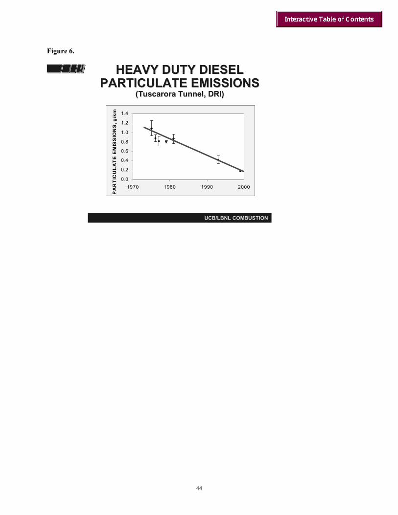
44

Figure 6.

UCB/LBNL COMBUSTION

HEAVY DUTY DIESEL HEAVY DUTY DIESEL PARTICULATE EMISSIONSPARTICULATE EMISSIONS

(Tuscarora Tunnel, DRI)(Tuscarora Tunnel, DRI)

0.0

0.2

0.4

0.6

0.8

1.0

1.2

1.4

1970 1980 1990 2000

PA

RTI

CU

LA

TE E

MIS

SIO

NS

, g/k

m

45

Difference Between Off-Road and On-Road Emissions

Terry L. Ullman Heavy-Duty Technology Assessment, Department of Emissions Research,

Southwest Research Institute Emissions from diesel engines are a function of the technology used, heavily influenced by the emission regulations in force for the engine model year. Therefore, emission regulations have a major influence on engine development and the engine emission signature. On-road diesel engines were regulated in 1979 using a steady-state process to characterize emissions of HC, CO, and NOx. Although particulate matter was not regulated, limits on smoke emissions were established for transient operation of the engine during accelerations, as well as for high load conditions. In 1984, gaseous emissions of on-road engines were regulated using a new transient cycle that included numerous accelerations, decelerations, idle, and limited motoring conditions in an effort to regulate on-road diesel engine emissions in a more realistic manner. In 1988, limits on particulate matter emissions were established. Since then, more restrictive limits on gaseous and particulate emissions have been established for on-road engines, as shown in Figure 1. As on-road emission regulations became more restrictive, the fuel sulfur level was limited to 500 ppm for 1991 and beyond, to assist diesel engine manufacturers in meeting the 0.25 g/hp-hr particulate emission limit. Largely due to emission regulations, on-road engines have developed differently than off-road engines. On-road engines of today are direct injected, turbocharged, aftercooled, use computer controlled fuel management along with high pressure fuel injection, and have good in-cylinder oil control; features that are only in limited use for current off-road engines. Some off-road engines use indirect injection and remain naturally aspirated. Off-road emission regulations took effect in 1996 and were phased in according to power level, using steady-state operation. It is planned that a transient cycle, representative of off-road equipment operation, will be used after 2007. It is likely that exhaust emission controls, such as EGR, catalyst, and particulate filter technologies, will be added to the state-of-the-art on-road engines of today to meet the more stringent regulations of 2007, which represent a 98 percent reduction from PM and NOx levels of the early 1980s. On-road and off-road engines also differ due to application. On-road engines ranging from 100 to 600 hp are used in trucks of various types, designed in common to work almost exclusively on roadways, placing the engine in front, with radiator, air intake, and exhaust positioned for optimum performance for typical roadway operation. Off-road engines are found in a variety of construction and agriculture equipment, as well as in welders, pumps, and generators, air compressors, and other off-road equipment. The breadth of off-road equipment is powered with engines that range from 5 to 750 hp. In several applications, the engine, radiators, air intake, and exhaust placement are optimized to meet the special requirements of the application. Fuel economy is important for both on-road and off-road engines. The sulfur level for on-road fuel was limited to 500 ppm in 1991 and will be reduced to 15 ppm for 2007. Off-road fuel is allowed to have sulfur levels to 5000 ppm, but in most cases, practical limitations on handling segregated fuel favors distribution of on-road fuel with red dye, to meet the needs of the off-road market. Off-road fuel may also be stored for much longer periods of time than on-road fuel due to intermittent use in some applications. Only after emission compliance is achieved, do both on-road and off-road engines have an opportunity to compete in their respective marketplace on the basis of fuel economy, performance, and cost. Figure 2 shows emissions from two on-road engines and one off-road engine plotted on the on-road and off-road regulatory space for NOx and PM. Recall that for on-road, the transient FTP cycle is required, designated with the letter "F" within the "Î" symbol used for the two on-road engines. Unlike

46

on-road emission regulations, off-road regulations are phased in by model year and power level. In the case of the 1995, 160 hp off-road engine, results from the 8-mode steady-state emission testing are given, designated with an "8". This off-road engine was tested over a backhoe-loader cycle, derived for off-road engine testing and designated with a "B" in the symbol "Î". In addition, the off-road engine was tested using the on-road transient FTP, designated with an "F". Note that the 1995, 160 hp off-road engine, designated by "" is not regulated. Emissions for three off-road engines are displayed in Figure 3. For each engine, results for the required 8-mode are given, along with results on the FTP transient and the backhoe-loader cycle given for comparison purposes. The 1997, 270 hp off-road engine had less than 6.9 g/hp-hr NOx and 0.4 g/hp-hr PM, complying with its respective 1996-2002 emission regulations for engines between 175 and 750 hp. The 2001, 420 hp, off-road emission results for the 8-mode, the FTP, and backhoe-loader cycles are also shown, designated with the "~". Although this engine's 8-mode results fall outside the compliance "box" given for 2001, 300-600 hp engines, the 420 hp rating represents a special case for this engine, which offers multiple, application-selectable ratings.

The data shown in Figure 3 illustrate that emission regulations force the implementation of engine technology to meet the tougher requirements as a condition to compete for market share. Transient cycle results for FTP or backhoe loader are higher in PM emissions and, except for the 1995 off-road engine, give higher NOx levels than were obtained over the 8-mode steady-state process. This points out that there can be significant differences in emissions with different engine operations. Although not shown, transient cycle HC and CO emissions can also be well above 8-mode steady-state levels.

As mentioned earlier, there can be a significant difference in sulfur levels between on-road and off-road fuels, although this difference is not universal. Figure 4 illustrates the increase in PM and change in NOx with a heavy black line extending from the respective engine/cycle point. Most of this increase in PM is due to sulfate emissions and associated water measured as PM in the process.

In addition to differences in NOx and PM between the off-road and on-road emissions, emission levels on 2-D fuel for 35 other compounds were compared. Table 1 lists all the FTP transient emissions that were notably different between on-road and off-road for the limited data set of two on-road and three off-road engines. Notably the means of two organic carbon compounds, chrysene and naphthalene, for the on-road and off-road engines were examined with respect to the level of soluble organic fraction of total PM. As shown in Table 2, the ratios of chrysene to SOF and naphthalene to SOF for off-road were both higher than for on-road, by a factor of 2. When the ratios were recomputed using soot, defined as total PM minus SOF, the ratios for off-road were both higher than for on-road, but this time, by a factor of 4 or 5. Although these ratios are based on a small data set, perhaps more rigorous analysis of a larger data set would yield more robust relationships to delineate differences between on-road and off-road engines. As time passes and on-road engine emissions are regulated to minute levels compared to off-road engines, soot emissions will be more strongly correlated to off-road engines. In summary, differences between on-road and off-road engine emissions exist because of engine technology, due to differences in engine application, fuel, competition, and mostly emission regulations. Off-road emissions of today are likely representative of on-road engine emissions of the past. Ratios of selected PAH-to-soot emissions may serve as indicators of off-road emissions. Finally, as on-road emissions approach zero beyond 2007, off-road engine activities may be indicated by the presence of soot (total PM-SOF).

47

Table 1. Emissions That Were Substantially Different Between On-Road and Off-Road, using 2-D Fuel

Table 2. Selected Ratios of Emissions That Show Difference Between Off-Road and On-Road

NOx

N2OBenzeneXyleneBenzo(a)anthraceneBenzo(a)pyreneBenzo(b)fluorantheneBenzo(k)fluoranthene

Off-Road Higher

Off-Road Lower6-Nitro benzo(a)pyrene

Benzo (g,h,i) peryleneChryseneIndeno (1, 2, 3-cd) pyreneAcenepthyleneFluorantheneNapthalene6-Nitro Chrysene

SOF Chrysene

Consider Off-Road On-RoadChrysene =SOF 2.3x10-5 1.2x10-5 2:1

SOF Napthlene Napthlene =SOF 0.6x10-5 0.3x10-5 2:1

PM - SOF SootChrysene

Soot 2.1x10-5 0.5x10-5 4:1

Consider

NapthleneSoot 0.5x10-5 0.1x10-5 5:1

Consider

After 2007 Soot May Become an Off-Road Signature

48

Figure 1. On-road transient emissions regulation space.

Figure 2. On-road and off-road regulation space.

0

0.1

0.2

0.3

0.4

0.5

0.6

0 1 2 3 4 5 6 7 8 9 10 11

Part

icul

ate,

G/H

P-H

R

NOx, G/HP-HR

1991

19941998

1990 (1988 CARB)

2002 (NOx + HC)

StandardsFor 2007

19841988

F

F

2001190 hp

1991350 hp

F - FTP Transient

0

0.1

0.2

0.3

0.4

0.5

0.6

0 1 2 3 4 5 6 7 8 9 10 11

Part

icul

ate,

G/H

P-H

R

NOx, G/HP-HR

BF

81991

19941998

1990 (1988 CARB)

(NOx + HC)2002

19841988

1996-2002 175<750 hp

1998-2002 50<175 hp

2004 50<100 hp

2003 100<175 hp

F

F

2001190 hp

1991350 hp

F - FTP Transient, 8 - 8 Mode S.S., B - Backhoe Loader

2001 300<600 hp

2003 175<300 hp2002 600<750 hp

1995160 hp

49

Figure 3. On-road and off-road engine emissions.

Figure 4. Effect of 2500 ppm sulfur fuel on on-road and off-road engine emissions.

0

0.1

0.2

0.3

0.4

0.5

0.6

0 1 2 3 4 5 6 7 8 9 10 11

Part

icul

ate,

G/H

P-H

R

NOx, G/HP-HR

BF

81991

19941998

1990 (1988 CARB)

(NOx + HC)2002

BF

BF

88F B

19841988

8

1996-2002 175<750 hp

1998-2002 50<175 hp

8

F

2001 300<600 hp 2001190 hp

1991350 hp


1995160 hp

1997270 hp

2001420 hp

0

0.1

0.2

0.3

0.4

0.5

0.6

0 1 2 3 4 5 6 7 8 9 10 11

Part

icul

ate,

G/H

P-H

R

NOx, G/HP-HR

BF

81991

19941998

1990 (1988 CARB)

(NOx + HC)2002

BF

BF

88F B

19841988

8

1996-2002 175<750 hp

1998-2002 50<175 hp

8

F

2001 300<600 hp 2001190 hp

1991350 hp


1995160 hp

1997270 hp

2001420 hp

51

Some Characteristics of Diesel and Gasoline Particulate Emissions

David Kittelson

Center for Diesel Research, Department of Mechanical Engineering, University of Minnesota

Introduction

Particle signatures from diesel and gasoline engines are briefly discussed here along with differences that might allow the two types of particles to be distinguished. Fundamental differences in PM formation processes in diesel and gasoline might offer hope for a particle signature. Some possible markers are briefly discussed here. They include particle size and particle composition. Most of the discussion focuses on the overall size and composition of particles from the two engine types. After these are presented the uniqueness of their signatures will be discussed briefly. This is not intended to be a literature survey, and only work done at the University of Minnesota is cited. Composition and Structure of Diesel Particulate Matter from Current Engines

The overall chemical composition of diesel particles is highly variable; however, the major constituents are always carbonaceous agglomerates (mainly elemental carbon [EC]), organic carbon (OC), sulfates, and ash. EC and OC are typically 80% or more of the particle mass. The OC/EC ratio generally decreases with load and is typically about 1:3 for highway cruise conditions.

Most of the particles emitted by engines are in the submicron diameter range, in two principal size modes: a nuclei mode containing most of the particle number in the 3 to 30 nm diameter range and an accumulation mode containing most of the particle mass in the 30 to 500 nm range. The nuclei mode typically contains less than 1% of the particle mass, but often more than 90% of the particle number. Nuclei mode particles consist primarily of volatile or semivolatile matter, mainly heavy organics and sulfur compounds. Solid metallic ash particles may also be present in this mode when metallic additives are used in the fuel or under very light load conditions in some engines. Most of the particle mass is found in the accumulation mode. Accumulation mode particles consist of carbonaceous agglomerates as well as adsorbed hydrocarbons and sulfates. Metallic ash from lubricating oil is also found in the accumulation mode.

The size and concentration of volatile and semivolatile particles emitted by diesel engines are strongly dependent upon dilution and sampling conditions. This is because the materials that comprise these particles (sulfur compounds and organics) are generally in the vapor phase in the tailpipe and undergo gas-to-particle conversion processes, nucleation, condensation, and adsorption, during dilution and cooling. These processes, especially nucleation, are highly nonlinear and extremely sensitive to conditions. As a result, dilution conditions, for example temperature and dilution rate, may change the concentration of particles in the nuclei mode by an order of magnitude or more. Conversely, solid particles, mainly carbon agglomerates and ash, are formed in the engine itself and thus not influenced by dilution conditions.

The size of the nuclei mode is usually sensitive to fuel sulfur content, but a significant nuclei mode may form even with very low-sulfur fuel and lubricating oil. Figure 1 shows some typical size distribution measurements made as a Cummins Engine Company funded extension of the DOE/CRC E-43 program (Kittelson et al., 2002b). These measurements were made with a Cummins ISM engine (1999 technology) running on specially formulated low-sulfur lubricating oil and fuels with sulfur content varying from 1 to 325 ppm. The same base fuel was used in all tests; fuel sulfur was varied with an additive. Four different operating conditions are shown: idle; light-medium load cruise (1400 rpm, 366 N-

52

m torque, 18% rated power); very light load cruise (1800 rpm, 154 N-m, 10% rated power); and heavy load cruise (1800 rpm, 776 N-m, 50% rated power). Measurements were made with and without a thermal denuder that removed all particles that evaporate at 300°C or less. The size distributions clearly show the submicron bimodal size distribution typical of diesel exhaust particles. The size of the mainly volatile nuclei mode is influenced by fuel sulfur, but that of the mainly solid accumulation mode is not. At idle the largest nuclei mode was observed with the 325 ppm sulfur fuel. The 26 and 1 ppm sulfur fuels gave smaller nuclei modes of essentially the same size. The thermal denuder reduced, but did not eliminate, the nuclei mode, indicating the presence of nonvolatile particles. At 1800 rpm, 154 N-m, the nuclei mode decreases, but does not disappear, as the sulfur content of the fuel is reduced. In this case, however, nuclei mode particles are nearly entirely removed by the thermal denuder, indicating that they are mainly volatile. At 1400 rpm, 366 N-m, a very large nuclei mode is present that is not strongly influenced by the sulfur content of the fuel. It is completely removed by the thermal denuder, indicating that it consists of volatile material. At 1800 rpm, 776 N-m, only the highest sulfur fuel, 325 ppm, exhibits a nuclei mode. Again, this mode is volatile and is removed by the thermal denuder. This series of tests reveals a complex behavior with respect to the fuel sulfur content, ranging from forming a large nuclei mode regardless of the fuel sulfur to only forming a nuclei mode with the highest sulfur fuel. A variety of physical and chemical methods were used to characterize the composition and size of diesel particles from modern engines as part of the CRC/DOE E-43 program (Kittelson et al., 2002a; Ziemann et al., 2002a; Sakurai et al., 2002; Tobias et al., 2001). A thermal desorption particle beam mass spectrometer (TDPBMS) was used to measure the volatility and mass spectra of the volatile fraction of all the particles in selected size ranges between 15 and 300 nm. Three different engines and fuels with sulfur contents from ~0 to 360 ppm were tested. For these engines and fuels, the organic component of total diesel particles and nanoparticles appeared to be mainly unburned lubricating oil. The major organic compound classes found were alkanes, cycloalkanes, and aromatics. Low-volatility oxidation products and PAHs that have been found in previous GC-MS analyses were only a minor component of the organic mass. Nanoparticles formed with 360 ppm sulfur fuel contained small amounts of sulfuric acid but those formed with fuels with less than 100 pm sulfur showed no evidence for sulfuric acid — the nanoparticles were nearly pure heavy organics. The physical properties of the particles were also studied using tandem differential mobility analyzers (TDMA). These experiments allowed size-resolved measurements of volatility and hygroscopicity to be made. In the volatility experiments the particles were heated and the shrinkage was monitored. For the hygroscopicity measurements the particles were humidified and their growth was monitored. The volatility measurements showed that diesel exhaust particles consist of an external mixture of more volatile and less volatile particles. At 30 nm, roughly the boundary between the nucleation and accumulation modes, both volatile and less volatile particles were found. For smaller sizes, volatile nuclei mode particles dominated; for larger sizes, less volatile carbonaceous agglomerates from the accumulation mode dominated. The volatile particles were found to evaporate in the TDMA like C24-C32 normal alkanes. These heavy alkanes are much more prevalent in lubricating oil than in fuel. The hygroscopicity measurements were used to estimate the concentration of sulfuric acid in the particles. Hygroscopic particles were observed with the 360 ppm sulfur fuel. The growth increased with decreasing particle size, suggesting that the smallest particles were enriched with sulfuric acid. The growth observed with the smallest particles tested, 6.5 nm diameter, was consistent with a sulfuric acid content of 20% by mass. The estimated mass fraction for 30 nm particles was only 5%. No detectable hygroscopic growth was observed for particles produced when the fuel sulfur content was less than 100 ppm.

Taken together, the size distribution, TDPBMS, and tandem DMA measurements led to several conclusions about the formation and composition of the nuclei mode. On the one hand, the size distribution measurements show that, in general, increasing the fuel sulfur increases the size of the nuclei mode. On the other hand, the TDPBMS and TDMA measurements show that the nuclei mode consists mainly of heavy hydrocarbons, with significant sulfuric acid found only in the smallest particles with the highest sulfur fuel. Thus it would appear that the presence of sulfur in the fuel facilitates the nucleation and growth of nuclei mode particles that consist of mainly heavy hydrocarbons. This same hypothesis was based solely on size distribution measurements and physical arguments by Khalek and coworkers

53

(2000). In most cases the nuclei mode contains less than 1% of the particle mass. Since DPM often contains 10% or more sulfate and water and 20 % or more OC, most of the sulfate and OC mass must reside in the accumulation mode, presumably adsorbed on the carbonaceous agglomerates formed by combustion. The nonvolatile material found in the nuclei mode at idle is likely to be ash formed from metallic additives in the lubricating oil. Emission standards for engines built for 2007 and beyond are so stringent that it will almost certainly be necessary to use exhaust filters. These filters are very effective at removing solid particles, so very little EC or ash is likely to leave the filters. Thus particles emitted by future trap-equipped engines are likely to consist of mainly volatile materials like sulfuric acid and heavy hydrocarbons. Many exhaust filters are catalyzed to facilitate combustion of collected particles. These catalysts are also effective at oxidizing SO2 in the exhaust to SO3, which reacts with water to form sulfuric acid. Consequently, the volatile particles emitted by such systems are likely to contain a higher fraction of sulfuric acid than currently observed, although the absolute concentrations will be low.

To summarize the findings on size and composition of diesel particles: • Diesel engines produce a bimodal size distribution in the submicron range with a nuclei mode

containing most of the particle number in the 3-30 nm diameter range and an accumulation mode containing most of the particle mass in the 30-500 nm range.

• Nuclei mode particles form mainly from volatile precursors, like heavy hydrocarbons from lubricating oil and sulfuric acid.

o Their formation is very dependent on dilution conditions, especially dilution rate and dilution air temperature.

o An insoluble core, probably related to lubricating oil metals, may be present in some cases, e.g., idle.

• The accumulation mode is where most “soot” or “smoke” resides o It consists primarily of carbonaceous agglomerates, adsorbed hydrocarbons, and sulfates. o It has been reduced sharply by better engine technology and may be nearly eliminated by

filtration. • Particles from future engines with exhaust filters are likely to consist of mainly volatile materials

like sulfuric acid and heavy hydrocarbons. Physical and Chemical Characteristics of Particles from Gasoline Engines

The mechanism of particle formation in gasoline engines is very different from that in diesels and not as well understood. In a gasoline engine, fuel and air are premixed before combustion and combustion takes place under chemically correct conditions. In a diesel engine combustion initially takes place in a fuel-rich jet that subsequently continues to oxidize as it mixes with air. The primary combustion process in a gasoline engine should not make particles. Particle formation in a gasoline engine results from local inhomogeneous conditions – fuel pooling, big droplets, cracks, crevices, etc. Formation is much more dependent on operating conditions than with diesel engines, increasing strongly at high loads. During cold starts, the fuel-air mixture in a gasoline engine is very rich, leading to significant EC formation. Gasoline “high emitters” with some combination of high oil consumption and rich operation may produce particles much like those from older diesel engines.

Gasoline engine exhaust particles are usually smaller than those emitted by diesel engines, mainly in the nuclei mode region (Graskow et al., 1998, 1999). They are often composed primarily of volatile and semivolatile materials, although ash may be the major constituent in some cases. Lube oil may play an important role in their formation. Most of the PM emitted under moderate operating conditions consists of so-called unresolved complex mixture, (a complex mix of organic carbon including branched and cyclic compounds) and ash.

New, well-maintained gasoline engines had very low PM emissions when warmed up, under moderate speed and load conditions (Graskow et al., 1998, 1999; Abdul-Khalek and Kittelson, 1995) but

54

were more sensitive to operating conditions than diesel and increased strongly at higher loads and with the richer mixtures that are associated with cold starts. Graskow and colleagues (1998) also showed that a catalytic converter did not effectively remove gasoline engine particles at high loads.

Studies of particle size and concentration on Minnesota highways (Kittelson et al., 2001 and 2003a) have shown that high concentrations of particles smaller than 50 nm diameter, nanoparticles, are present over gasoline-dominated roadways. Concentrations of both nuclei mode and accumulation mode particles were higher in the presence of diesel traffic, but road speed was observed to have more influence on nanoparticle concentrations, than vehicle mix, with high speed leading to higher concentrations. Some of this effect was attributed to storage of volatile nuclei mode precursors in the exhaust system during low speed operation and their subsequent release under high speed and load conditions that lead to high exhaust temperatures. The main influence of diesel traffic was an increase in the concentration of particles in the accumulation mode range.

In a recent DOE study Kittelson and others (2003b) measured particle mass, chemical composition, number, surface area, and size for a small fleet of gasoline vehicles consisting of nearly new “low emitters” and older “high emitters.” Measurement conditions included on-road chase experiments; on-road urban fleet, weekday, and weekend measurements; chassis dynamometer tests involving hot and cold unified cycles and steady operation at idle, 20, 35, 65, and 70 mph; outdoor Minnesota cold start and idle tests; and engine dynamometer tests of a simulated high emitter. The work supports earlier observations of very low PM emissions from modern, well-maintained gasoline engines under normal cruise conditions. However, under very high load or cold start conditions, these emissions increase dramatically. High speeds led to high nanoparticle emissions, especially after a period of low speed operation. This was attributed to storage of nanoparticle precursors at light load and their subsequent release under high speed, high exhaust temperature conditions. Number emissions at 70 mph ranged from 1011 to 1015 particles per mile. This is in the same range as reported for on-road measurements in Minnesota (Kittelson et al., 2001, 2003a).

Chemical compositions of particles emitted under several operating conditions were also determined. High elemental carbon emissions, ranging from 40% to 70% of the emitted mass, were observed during 0°C cold start unified cycles, even with modern ‘low emitters.” This study also showed that a gasoline engine with high oil consumption produced a diesel-like particle size distribution with higher nuclei mode concentrations than typical modern diesel engines. Two Possible Markers for Diesel and Gasoline PM Are Size and Bulk Composition

• New well-maintained gasoline engines operating under moderate speed and load conditions emit low concentrations of very small particles. The ratio of the concentration of particles in the nuclei mode to that in the accumulation mode is higher than for diesel engines. This might offer promise as part of a particle signature. Unfortunately, gasoline high emitters and even normal emitters when operating under very high load, or rich cold start conditions, produce size distributions that are similar to diesel.

• EC is sometimes used as a marker for diesel but has many other sources including gasoline engines. Under 0°C cold start conditions even modern well-maintained gasoline engines may emit particles containing 40% to 70% EC. Gasoline high emitters may also be associated with high EC emissions.

• Both size and EC are likely to be better markers in roadside freeway samples than in area samples because vehicles on such roadways are more likely to be operating under warmed-up, cruise conditions.

• Both diesel and high emitting gasoline engines emit particles with a significant fraction derived from lube oil. Organics and metals from lube oils provide markers for such engines, but diesel and gasoline oils contain similar constituents. Lube oil components are a marker for particles

55

produced by piston engines but are unlikely to be suitable for differentiating between different engine and fuel types.

• Future diesel engines equipped with exhaust filters will have very different particle signatures and will likely consist mainly of sulfates and heavy hydrocarbons with little or no EC or ash.

Other Markers That Might Be Considered

• Rare earth metals have been used in Austria as a tracer for diesel. If an area of the US could be identified where most of the diesel fuel used came from local supplies, experiments with doped diesel fuel might yield useful information.

• The ratio of NO2 to CO is much higher in diesel exhaust than in gasoline exhaust. This ratio changes quickly away from roadways but might be a useful marker near them.

References Abdul-Khalek, I.S. and D.B. Kittelson, 1995. "Real Time Measurement of Volatile and Solid Exhaust

Particles Using a Mini-Catalyst," SAE Paper No. 950236, SAE International Congress & Exposition, Detroit, MI, February 27-March 2, 1995.

Graskow, B.R., D.B. Kittelson, I.S. Abdul-Khalek, M.R. Ahmadi, and J.E. Morris. “Characterization of Exhaust Particulate Emissions from a Spark Ignition Engine,” SAE Paper No. 980528 and SP-1326 also in 1998 Transactions of the Society of Automotive Engineering, Vol. 3, Engine, Fuels and Lubricants, 1998.

Graskow, B.R., D.B. Kittelson, M.R.Ahmadi, and J.E. Morris. 1999. “Exhaust Particulate Emissions from Two Port Fuel Injected Spark Ignition Engines,” SAE Paper No. 1999-01-1144, 1999.

Khalek, I.A., D.B. Kittelson, and F. Brear. 2000. "Nanoparticle Growth During Dilution and Cooling of Diesel Exhaust: Experimental Investigation and Theoretical Assessment," SAE Paper No. 2000-01-0515, 2000.

Kittelson, D.B, W. Watts, and J. Johnson, 2002a. “Diesel Aerosol Sampling Methodology,” Final Report, CRC Project E-43, August 2002.

Kittelson, D, W. Watts, J. Johnson, N. Bukowiecki, M. Drayton, D. Paulsen, Q. Wei, A. Ng, and H-J. Jung, 2002b. “Diesel Aerosol Sampling Methodology - CRC E-43 Cummins Final Report,” October 2002.

Kittelson, D.B., W.F. Watts and J. P. Johnson, 2001. “Fine Particle (Nanoparticle) Emissions on Minnesota Highways.” Final report submitted to Minnesota Department of Transportation, 2001.

Kittelson, D.B., W.F. Watts and J. P. Johnson, 2003a. “Nanoparticle Emissions on Highways,” manuscript in preparation for submission to Atmos. Environ., 2003.

Kittelson, D.B., W.F. Watts, J. P. Johnson, and J. Schauer, 2003b. “Gasoline Vehicle Exhaust Particle Sampling Study,” final report in preparation for submission to U. Dept of Energy, June 2003.

Sakurai, H., H.J. Tobias, K. Park, D. Zarling, K.S. Docherty, D.B. Kittelson, P.H. McMurry, and P.J. Ziemann, 2002. “On-Line Measurements of Diesel Nanoparticle Composition, Volatility, and Hygroscopicity,” Submitted to Atmos. Environ., 2002.

Tobias, H.J., D.E. Beving, and P.J. Ziemann, H. Sakurai, M. Zuk, P.H. McMurry, D. Zarling, R. Waytulonis, and D.B. Kittelson. 2001. "Chemical Analysis of Diesel Engine Nanoparticles Using a Nano-DMA/Thermal Desorption Particle Beam Mass Spectrometer," Environ. Sci. Technol. 2001, 35, 2233–2243.

Ziemann, P.J., H. Sakurai, and P.H. McMurry, 2002. “Chemical Analysis of Diesel Nanoparticles Using a Nano-DMA/Thermal Desorption Particle Beam Mass Spectrometer,” Final Report, CRC Project No. E-43-4, April 2002.

Figu

re 1

. Par

ticle

size

dis

tribu

tions

mea

sure

d w

ith a

Cum

min

s ISM

eng

ine

(199

9) ru

nnin

g w

ith lo

w su

lfur l

ubric

atin

g oi

l and

var

ying

fuel

sulfu

r lev

els.

TD

indi

cate

s tha

t a th

erm

al d

enud

er o

pera

ting

at 3

00°C

was

use

d to

rem

ove

vola

tile

parti

cles

. Not

e th

at th

e nu

clei

mod

e is

usu

ally

sens

itive

to fu

el su

lfur c

onte

nt, b

ut

a si

gnifi

cant

nuc

lei m

ode

may

form

eve

n w

ith v

ery

low

sulfu

r fue

l and

lube

oil.

1.00

E+05

1.00

E+06

1.00

E+07

1.00

E+08

1.00

E+09

1.00

E+10

110

100

1000

dN/dlogDp, part/cm3

325

ppm

S26

ppm

S1

ppm

S1

ppm

S w

ith T

D

Cor

rect

ed fo

r DR

Not

cor

rect

ed fo

r pa

rtic

le lo

sses

ISM

eng

ine,

Idle

1.00

E+05

1.00

E+06

1.00

E+07

1.00

E+08

1.00

E+09

1.00

E+10

110

100

1000

dN/dlogDp, part/cm3

325

ppm

S49

ppm

S26

ppm

S32

5 pp

m S

with

TD

Cor

rect

ed fo

r DR

Not

cor

rect

ed fo

r pa

rtic

le lo

sses

ISM

eng

ine,

18

00 rp

m, 1

54 N

-m

1.00

E+05

1.00

E+06

1.00

E+07

1.00

E+08

1.00

E+09

1.00

E+10

110

100

1000

Dp

(nm

)

dN/dlogDp, part/cm3

325

ppm

S49

ppm

S26

ppm

S1

ppm

S32

5 pp

m S

with

TD

Cor

rect

ed fo

r D

RN

ot c

orre

cted

for

part

icle

loss

es

ISM

eng

ine,

14

00 rp

m, 3

66 N

-m

1.00

E+05

1.00

E+06

1.00

E+07

1.00

E+08

1.00

E+09

1.00

E+10

110

100

1000

Dp

(nm

)

dN/dlogDp, part/cm3

325

ppm

S49

ppm

S26

ppm

S32

5 pp

m S

with

TD

Cor

rect

ed fo

r D

RN

ot c

orre

cted

for p

artic

le lo

sses

ISM

eng

ine,

18

00 rp

m, 7

76 N

-m

1.00

E+05

1.00

E+06

1.00

E+07

1.00

E+08

1.00

E+09

1.00

E+10

110

100

1000

dN/dlogDp, part/cm3

325

ppm

S26

ppm

S1

ppm

S1

ppm

S w

ith T

D

Cor

rect

ed fo

r DR

Not

cor

rect

ed fo

r pa

rtic

le lo

sses

ISM

eng

ine,

Idle

1.00

E+05

1.00

E+06

1.00

E+07

1.00

E+08

1.00

E+09

1.00

E+10

110

100

1000

dN/dlogDp, part/cm3

325

ppm

S49

ppm

S26

ppm

S32

5 pp

m S

with

TD

Cor

rect

ed fo

r DR

Not

cor

rect

ed fo

r pa

rtic

le lo

sses

ISM

eng

ine,

18

00 rp

m, 1

54 N

-m

1.00

E+05

1.00

E+06

1.00

E+07

1.00

E+08

1.00

E+09

1.00

E+10

110

100

1000

Dp

(nm

)

dN/dlogDp, part/cm3

325

ppm

S49

ppm

S26

ppm

S1

ppm

S32

5 pp

m S

with

TD

Cor

rect

ed fo

r D

RN

ot c

orre

cted

for

part

icle

loss

es

ISM

eng

ine,

14

00 rp

m, 3

66 N

-m

1.00

E+05

1.00

E+06

1.00

E+07

1.00

E+08

1.00

E+09

1.00

E+10

110

100

1000

Dp

(nm

)

dN/dlogDp, part/cm3

325

ppm

S49

ppm

S26

ppm

S32

5 pp

m S

with

TD

Cor

rect

ed fo

r D

RN

ot c

orre

cted

for p

artic

le lo

sses

ISM

eng

ine,

18

00 rp

m, 7

76 N

-m

57

Morphological Aspects of Combustion Particles

Douglas A. Blom, John M.E. Storey, and R.L. Graves Oak Ridge National Laboratory

The high spatial resolution imaging and analytical information available from transmission

electron microscopy (TEM) is well suited to the characterization of individual combustion particles. TEM provides information on the morphology, crystal structure, and elemental composition of PM from the nanometer to micron level. Most often, scanning electron microscopy (SEM) is performed on combustion particles collected on filters. SEM of filter-bound particles gives little information about the size and shape of individual particles. By obtaining a representative sample of individual particles, it may be possible to come up with mathematical descriptions of their morphology, density, and size. Models that examine the impact of airborne particles on the lungs could thus have much better representations of combustion particles. This would improve greatly the understanding of the health impacts of atmospheric particles.

As part of an ongoing research project into the health effects of motor vehicle particulate matter, Southwest Research Institute (SWRI) performed chassis dynamometer tests of vehicles with spark ignition and compression ignition engines. They utilized the unified driving cycle, derived from the US EPA’s Federal Test Procedure, in their tests of the vehicles. PM was collected from three different portions of that cycle: the initial cold-start idle, a high-speed cruise event, and a hot idle event.

SWRI agreed to sample the exhaust stream from a number of different vehicles for TEM examination. The vehicle exhaust was passed through a dilution tunnel to stop the agglomeration of the PM and simulate the effect of the exhaust exiting the tailpipe. Two methodologies are commonly used to collect PM for characterization: filters and impactors. Filters are used mostly for measuring the weight of the PM emitted at different points in a drive cycle. Wet chemistry methods can extract the soluble fraction of the PM for chemical analysis. These filtration and extraction methods do not preserve the particle morphology or provide spatially resolved chemical information. Impactor methods can be adapted to provide samples appropriate for TEM examination. By collecting for short times, we were able to preserve the initial shape of the particles. TEM grids coated with thin holey carbon films are available to serve as the support substrate. A line was run from a sampling port on the dilution tunnel to a micro-orifice uniform deposit impactor (MOUDI) (Marple et al 1991). Copper TEM grids coated with a holey amorphous carbon film were placed on different stages of the MOUDI. PM was collected from the following vehicle types: current technology, gasoline-fueled, spark ignition vehicle; current technology, diesel-fueled, compression ignition light-duty vehicle; current technology, diesel-fueled, compression ignition pickup (engine-certified on heavy-duty cycle); pre–emission control, gasoline-powered vehicle using both unleaded and leaded fuels; and an advanced technology, gasoline-fueled, spark ignition, direct injection vehicle.

Typical “particles” from the current technology, gasoline spark ignition vehicle are seen in Figure 1. The thin carbon support film stretches from lower left to upper right across the micrograph with two holes on either side. Figure 2 is a higher magnification micrograph illustrating how each particle is composed of a number of small spheres linked together to form a three-dimensional object. This is the dominant morphology of combustion particulate matter. The primary particles are typically between 30 and 60 nm in diameter. Figure 3 shows the turbostratic crystal structure commonly observed. The contrast in the image is created by diffraction of the electrons from the various planes of atoms. The carbon atoms form sheets that are all perpendicular to the surface of the particle, but without long-range order among the sheets. This crystal structure is observed for most moderate temperature combustion events. Figure 4 is a high resolution micrograph of a particle that is graphitic in nature. The faceting and long-range order are clearly seen in the micrograph. This particular particle was formed via a much higher temperature combustion event.

Figure 5 is a typical exhaust particle collected from the light-duty diesel vehicle. The overall morphology and turbostratic crystal structure are very similar to those of gasoline vehicle PM. A diesel

58

engine in a pickup truck certified on the heavy-duty cycle emitted the PM seen in Figure 6. The inset is a lower magnification micrograph illustrating typical morphology from this vehicle-engine combination.

The emissions from a 1967 Chrysler 300 were collected and characterized as part of a program investigating the historical trends of PM emission. Figure 7 shows typical PM. The morphology is very similar to that of PM emitted by modern gasoline engines. Figure 8 illustrates the PM emissions from this same vehicle when operated on leaded fuel. Note the large crystalline particle embedded in the carbonaceous PM. Figure 9 is an energy dispersive X-ray spectroscopy (EDS) spectrum from the particle shown in Figure 8. The high-energy electrons as they pass through the thin sample sometimes remove a valence electron from the sample. An electron from a higher energy shell of the atom relaxes into the lower energy state by emitting an X-ray photon. Because the energy differences between electronic states in atoms are well known, measuring the X-rays emitted from a sample during electron irradiation provides a measurement of the chemical composition of the sample. The leaded fuel PM contains carbon, oxygen, lead, and bromine. The lead and bromine are byproducts of the lead additive used.

A vehicle containing an advanced technology, spark ignition, direct injection engine produced the particulate matter in Figure 10. Of special note is the apparent bimodal distribution of the primary carbon particle size. One set of particles is made up of primary spheres that are 10 nm in diameter, while the other particles are more similar to traditional gasoline and diesel particles with a primary particle size between 30 and 60 nm.

Particulate matter from a variety of in-use and test vehicles has been collected for TEM characterization. Well-designed sampling methods are required to provide a specimen that maintains the geometry and composition of the source emissions. Most solid PM from combustion processes is carbonaceous and consists of chains of turbostratic carbon spheres linked together in a complex three-dimensional way. TEM provides very high spatial resolution information on the structure, arrangement and elemental composition of individual emission particles. The carbonaceous fractions of PM from the various vehicles are quite similar in general, although some of the details vary according to engine and emission control technology. References V. P. Marple et al., Aerosol Science and Technology, 14, 434–446, 1991.

Figure 1. Low magnification micrograph of motor vehicle PM. The chain-like objects are the PM on top of the amorphous carbon support film. On either side is a hole.

Figure 2. Micrograph of motor vehicle PM showing the size of the component carbon spheres.

Figure 3. High resolution electron micrograph showing the turbostratic crystal structure common for combustion particles.

Figure 4. Graphitic emission particle formed via high temperature combustion.

Figure 5. Turbostratic PM typically observed from a light-duty diesel vehicle.

Figure 6. Particulate matter emitted by a heavy-duty certified diesel engine in a light truck.

60

Figure 7. PM from a pre–emission control vehicle running on unleaded gasoline.

Figure 8. PM emitted from a pre–emission control vehicle burning leaded gasoline.

Figure 9. EDS spectrum from the particle seen in Figure 8. The particle is composed of C, O, Pb and Br. The Cu signal detected is a background signal from the Cu support grid.

61

Figure 10. PM emitted from an advanced technology, gasoline-powered vehicle.

63

Characterization of Vehicle Emissions and Urban Aerosols by an Aerosol Mass Spectrometer

Douglas R. Worsnop, Manjula Canagaratna, and John Jayne

Aerodyne Research, Inc.

Jose Jimenez University of Colorado

Over the last several years a new Aerosol Mass Spectrometer (AMS) has been developed for real-

time measurement of size-resolved chemical composition of submicron atmospheric aerosol (Jayne et al., 2000b). In multiple deployments of the AMS worldwide clear patterns in aerosol chemistry have been observed, distinguishing primary and secondary aerosol chemistry (Allan et al., 2003a, 2003b; Jiménez et al., 2003). Small organic particles (<200 nm diameter) are consistently observed in urban areas while larger (> 200 nm) particles appear to be composed of organic/sulfate mixtures, which are associated with regional evolution and transport of aerosol. Based on direct characterization of the size and chemical composition of vehicle aerosol emissions, the small organic mode is identified as primary combustion soot aerosol.

We believe AMS monitoring of this small organic mode can provide a tracer of local vehicle-derived aerosol levels. Below we briefly describe the operation of the AMS and then describe results from PM2.5 Technology Assessment and Characterization Study in New York City (PMTACS-NY; Project description is available at www.asrc.cestm.albany.edu/pmtacsny). Two AMS instruments were deployed during July 2000: vehicle chasing observations (Aerodyne Research, Inc.) measured emission factors of individual on-road vehicles (Canagaratna et al., manuscript in preparation) while monitoring at a fixed site (SUNY Albany) provided continuous ambient aerosol loadings (Drewnick et al., 2002a, 2000b). Taken together, these results provide a picture of the role of combustion soot aerosol in ambient aerosol in an urban environment.

A schematic of the AMS is shown in Figure 1. The AMS uses an aerodynamic lens to sample submicron particles (between 0.03 and 1.5 µm vacuum aerodynamic diameter) into vacuum, where they are aerodynamically sized, thermally vaporized on a heated surface, and chemically analyzed via electron impact (EI) ionization quadrupole mass spectrometry (Jayne et al., 2000a). Results from measurements obtained at a variety of field campaigns show that the AMS has the potential to quantitatively measure size-dependent volatile and semivolatile chemical compositions, including most organic carbon (OC) and inorganic (acid, salt) components for the aerosol ensemble, with limited single-particle information (Allan et al., 2002a; Drewnick et al., 2002a; Jimenez et al., 2003). The AMS operates in two modes. In time-of-flight (TOF) mode aerosol size distributions are determined at several preselected fragment ions using a beam-chopping technique. In mass spectrum (MS) mode, the chopper is moved out of the particle beam and ensemble mass spectra (0-300 amu) are obtained for the sampled aerosol. Depending on the type of experiment, the AMS is alternated between the MS and TOF modes at time intervals of 2 to 30 seconds.

Detection is performed by directing the particle beam onto a resistively heated surface under high vacuum (~ 10-8 Torr). Upon impaction, the volatile and semivolatile components in/on the particles flash vaporize. The vaporization source is integrally coupled to an electron impact ionizer at the entrance of a quadrupole mass spectrometer as shown in Figure 2. The separation of the vaporization and ionization steps is essential to the aerosol mass quantification that is possible with the AMS. Since the AMS requires aerosol species to be vaporized in order to be detected, this technique does not detect refractory components whose vapor pressure is very low at the temperature of the AMS vaporizer (~ 550oC), such as mineral dust or elemental carbon (EC) aerosols. However, volatile/semivolatile components internally mixed with nonvolatile aerosol components can be detected by the AMS. For example, recent measurements during the ACE-Asia campaign have shown that while most mineral dust particles could not be detected by the AMS, Ca(NO3)2 on these particles could be detected (Bower et al., 2002).

64

Analysis of MS signatures (based on comparison with standard EI mass spectral libraries, as well as laboratory calibrations) easily distinguishes inorganic (e.g., ammonium, nitrate, sulfate) and organic species. Detailed identification of organic components is not possible from EI mass spectra, which are composed of overlapping ion fragmentation patterns from complex mixtures. However, organic composition can be classified (distinguishing hydrocarbon and oxygenated hydrocarbon classes, for example) by comparing the chemically resolved aerosol size distributions measured for different organic signature fragments in the TOF mode. Source Characterization Experiments

Aerosol emissions from mobile sources were characterized during PMTACS-NY by “chasing” in-use vehicles with the Aerodyne mobile laboratory, which was instrumented with the AMS and a suite of other gas-phase measurements. Aerosol emission indices, including chemical composition and size distributions of the exhaust aerosol, were measured for each vehicle that was chased (together with emission indices for NOx and other gas-phase species).

Figure 3 shows an example of data collected while chasing an individual New York City bus. The plot shows the time trend of total volatile particulate matter (2-second resolution, measured with the AMS) as well as analogous trends in the 1-second measurements of CO2 mixing ratio, total particle number concentration, and mobile lab speed during a single vehicle chase event. The mobile lab speed is a proxy for the target vehicle’s speed. The baseline signal levels in the gas and particle time trends represent ambient concentrations of the various species during the chase event. The peaks in the particle and gas-phase signals, which last for approximately 10-20 seconds, represent separate instances during the chase when the sampling inlet of the mobile lab continuously captured the target vehicle’s exhaust plume. Thus, one vehicle chase is made up of a series of “plume captures” that average emissions from the target vehicle over a range of driving conditions.

Emission Ratios

Since CO2 is a tracer for the dilution of the exhaust plume, the correlation of PM and CO2 measurements (evident in Figure 3) is key to this experiment. A PM emission index that is referenced to CO2 can be converted to a fuel-use-based emission index because CO2 emissions are proportional to fuel burned. Figure 4 shows a linear fit of the PM mass vs CO2 concentration over the entire chase event. This fit is performed with the intercept fixed at representative ambient CO2 and PM values for the event. The single emission index determined from a chase event characterizes the average PM emission characteristics of the given vehicle over the entire measurement time period.

Figure 5 summarizes the results of all the emissions ratios calculated in this study categorized by vehicle type. The height of the bar denotes the average emission ratio calculated over all the relevant chase events that represent the particular vehicle class, while the error bar represents one standard deviation of the mean (calculated for the number of vehicles sampled, as labeled). The vehicle classes sampled include NYC Metropolitan Transit Authority (MTA) buses, non-MTA buses, and other heavy-duty vehicles. “Non-MTA buses” consist of passenger buses used in the city that are operated by companies other than the MTA. The “other heavy-duty” vehicle category contains trucks as well as school and charter buses. In general, Figure 5 indicates that passenger buses have lower emission ratios than coach and school buses and heavy-duty trucks. It is of interest to note that the dirtiest vehicle sampled was a “smoking” car, with an emission factor 10 times higher than that from a typical diesel vehicle. Within the MTA fleet, it appears that the newer diesel engine technology (Series 50) is cleaner than the older technology (6V_92). Likewise, diesel buses with CRT (continuously regenerating technology) trap systems and nondiesel buses fueled by CNG (compressed natural gas) are much cleaner than traditional diesel buses. It is important to note that the emission indices shown in Figure 5 do not include black carbon (not measured by the AMS), which typically represents more than one half of the total organic emission. Overall, the measured emission indices are consistent with reported values for organic carbon in the literature (Allan et al., 2000; Kirchstetter et al., 1999). For reference, the tunnel

65

measurements by Kirchstetter et al. (1999) of PM2.5 emissions from trucks and gasoline vehicles are plotted on the right side of Figure 5.

Chemical Composition

The majority of studies of exhaust aerosol chemical composition have involved collection of the particles on filters followed by solvent extraction and GC-MS analysis of the resulting chemical species (Rogge et al., 1993; Schauer et al., 1999, 2002). In these studies, only 5% to 10% of the elutable particulate mass can be resolved and speciated. The rest of the eluted particulate mass is usually referred to as unresolved complex mixture (UCM) and is not speciated. Recent measurements by Tobias and colleagues (2001), in which a Thermal Desorption Particle Beam Mass Spectrometer (TDPBMS) was used to study particles emitted by a heavy-duty diesel engine operating under heavy and light-load laboratory conditions, have shown that for the conditions under which the experiment was operated, the volatile component of diesel aerosol was at least 95% unburned lubricating oil.

The detection scheme used by the AMS is very similar to the TDPBMS, so that mass spectral signatures measured by the two instruments can be directly compared. Figure 6 shows the mass spectrum obtained by averaging the exhaust fuel mass spectra obtained over many diesel vehicle chase events. The exhaust fuel spectrum for each chase event was obtained by taking the difference between the average mass spectrum obtained during plume captures in the event and the average mass spectrum obtained during background sampling time periods. All spectra are dominated by the ion series CnH2n+1

+ (m/z 43,57,71,85, …), which is typical of normal and branched alkanes; in addition, the series CnH2n-1

+ (m/z 41,55,69,83, …) and CnH2n-3

+ (m/z 53,67,71, …), typical of cycloalkanes, and C6H5CnH2n+ (m/z

77,91,105,119…), typical of aromatics, are observed. In the study by Tobias and colleagues, the ratio of the alkane to cycloalkane series in the m/z 41-43, 53-57, 67-71 and m/z 81-85 ranges was used to distinguish the condensed fuel/lubricant oil ratio in the aerosol. In particular, the increasing dominance of the cycloalkane series compared to the normal/branched alkane series within the m/z 67-71 and m/z 81-85 range were used as strong signatures of a high lubricant oil/fuel ratio. These trends, which have also been observed in laboratory AMS studies of pure lubricant oil aerosols, are observed in Figure 6. This suggests, as observed in TDPBMS study (Tobias et al., 2001), that under most operating conditions the organic carbon fraction of in-use diesel vehicle exhaust aerosol is dominated by condensed lubricant oil.

Size Distribution

It is known that diesel exhaust particle size distributions are typically trimodal with a small nano mode (0-50 nm), an accumulation mode (50-500 nm), and a larger coarse mode. While the nano mode dominates number-weighted size distributions, the accumulation mode accounts for most of the PM mass and dominates the mass-weighted size distributions. Since the AMS provides mass-weighted aerodynamic size distributions for submicron aerosol, these measurements are expected to be most sensitive to the accumulation and coarse modes of the exhaust aerosol. Sensitivity to the coarse mode is limited by reduced aerosol focusing in the aerodynamic lens for large particle sizes (> 600 nm).

Figure 7 shows an average of the chemically resolved mass distributions provided by the AMS during the chase events shown in Figure 3. Size distributions of both sulfate and organic-containing aerosols are displayed. For each species separate size distribution averages were obtained according to a CO2 concentration-based data processing filter that defined time periods which distinguished “in-plume” sampling from the ambient background aerosol. These size distributions are plotted as solid and dotted curves in Figure 7, respectively.

Observed increases of a few hundred ppm CO2 (see x-axis of Figure 4) correspond to about a 1000-fold dilution of the exhaust plume in the atmosphere. Thus, as is clear in Figure 7, the “in-plume” size distributions are a combination of both exhaust and ambient aerosol; the vehicle emission is given by the difference between the solid and dotted lines. For example, the sulfate ambient mass loading dominates the larger mode (vacuum aerodynamic diameter ~ 400 nm), but vehicle emissions dominate the smaller mode (~90 nm). For organics the “in-plume” mass loading is larger than both the small and large mode ambient background loading. The similar aerodynamic size of the “in-plume” sulfate and organic

66

mass distributions (particularly for the small 90-nm mode) suggests that the two species are internally mixed in the exhaust aerosol. The AMS cannot definitively confirm the state of mixing, however, because it measures the ensemble aerosol rather than single particles.

Ambient Aerosol Measurements The vehicle emission results can be related directly to ambient measurements taken during the same period in New York City during PEMTACS (Drewnick et al., 2002a, 2002b). Figure 8 shows a speciated mass distribution averaged over the month of July (2000). This distribution is typical of observations in a number of urban environments (Allan et al., 2003a, 2003b; Jiménez et al., 2003). AMS ambient mass distributions typically consist of two modes: one small mode that peaks at a vacuum aerodynamic diameter of ~100 nm and a large mode that peaks at ~ 400 nm. The similarity between the dotted curves in Figure 7 and the curves in Figure 8 is consistent with the fact that they are both measurements of urban ambient aerosol distributions. As noted above, the small mode is dominated by organics while the large mode is typically a mixture of sulfate and organics. The small mode peaks in the morning hours, decreases in the afternoon, and then rises again in the evening, reaching another peak around midnight. This pattern likely reflects peaks in vehicle emissions during morning rush hour, followed by rising and lowering boundary-layer height in the afternoon and evening, respectively.

The mass distribution of the small ambient mode is very similar to that in the vehicle chase plumes. Furthermore, during periods with large contributions from the small mode, the aerosol mass spectra contain long hydrocarbon ion-series that are characteristic of vehicle exhaust aerosol. In contrast, during the afternoon period, when the larger particles are more dominant, the mass spectra are dominated by an organic fragment (m/z 44, CO2

+) that is a signature of oxidized, secondary organic species. This same pattern has been observed in multiple urban and rural environments.

Summary

The similarity between the size distributions and mass spectra of the small-mode aerosol and the exhaust aerosol, when combined with the correlation between small-mode time trends and traffic activity, indicates that in AMS ambient aerosol measurements, the small-mode aerosol provides a clear signature of motor-vehicle-related aerosol. In contrast, the larger aerosol mode, largely composed of sulfate and secondary organics, appears to be associated with regional aerosol processing and transport. The larger mode is relatively more important in summer versus winter, presumably reflecting levels of photochemical activity; while the smaller mode is favored on days with low wind, when accumulation of local emissions is enhanced (Allan et al., 2002a, 2002b). Further studies are underway to more quantitatively evaluate the primary/secondary distribution of the organic carbon in both the mass spectra and size distributions. The combination of in-use vehicle emission measurements with ambient sampling of aerosol loading provides a powerful tool for characterizing the contribution of vehicle particle emissions to ambient aerosol mass loading. It is important to note that AMS detects only organic carbon; black carbon measurement requires other techniques. It is also important to note that the AMS measurements cannot resolve the contributions of gasoline and diesel emissions. As has been observed by others, both the chemistry and microphysics of the particles emitted from both vehicle types appear to be indistinguishable, i.e., hydrocarbon (oil)–like mass spectra dominated by sub-100-nm particle diameters. The typical gasoline vehicle has lower emission factors, which are counter-balanced by the larger number of gasoline vehicles in the total contributing to ambient loading. It is not clear whether the on-road mobile sampling approach presented here is capable of sampling sufficient numbers of vehicles to statistically evaluate the relative contributions of different vehicle types to the ambient aerosol. However, the AMS ambient aerosol loading data, represented by Figure 8, give a quantitative signature of the contribution of vehicle emissions to the local environment.

67

References Allan, J.D., H. Coe, K.N. Bower, P.I. Williams, M.W. Gallagher, M.R. Alfarra, J.L. Jimenez, D.R. Worsnop, J.T.

Jayne, M.R. Canagaratna, E. Nemitz, and A.G. McDonald, Quantitative Sampling Using an Aerodyne Aerosol Mass Spectrometer. Part 2: Measurements of Fine Particulate Chemical Composition in Two UK Cities., Journal of Geophysical Research – Atmospheres, in press, 2002a.

Allan, J.D., H. Coe, K. N.Bower, P.I. Williams, M.W. Gallagher, M.R. Alfarra, J.L. Jiménez, D.R. Worsnop, J.T. Jayne, M.R. Canagaratna, E. Nemitz, and A.G. McDonald, Quantitative Sampling Using an Aerodyne Aerosol Mass Spectrometer. Part 1: Techniques of Data Interpretation and Error Analysis, J. Geophys. Res., in press, 2003a.

Allan, J.D., J.L. Jiménez, H. Coe, K.N. Bower, P.I. Williams, M.W. Gallagher, and D.R. Worsnop, Quantitative Sampling Using an Aerodyne Aerosol Mass Spectrometer. Part 2: Measurements of Fine Particulate Chemical Composition in Two UK Cities, J. Geophys. Res., in press, 2003b.

Allan, J.D., J.L. Jimenez, H. Coe, K.N. Bower, P.I. Williams, and D.R. Worsnop, Quantitative Sampling Using an Aerodyne Aerosol Mass Spectrometer. Part 1: Techniques of Data Interpretation and Error Analysis., Journal of Geophysical Research – Atmospheres, in press, 2002b.

Allan, J.D., P.R. Mayo, L.S. Hughes, L.G. Salmon, and G.R. Cass, Emissions of Size-Segregated Aerosols from On-Road Vehicles in the Caldecott Tunnel, Env. Sci. and Tech., 35, 4189–4197, 2000.

Bower, K.N., T.W. Choularton, H. Coe, J.D. Allan, R. Burgess, M.C. Facchini, M.R. Alfarra, D. Topping, P.I. Williams, and G.B. McFiggans, Aerosol-Cloud Interactions in ACE-Asia, in Abstracts of the 21st Annual AAAR conference, pp. 128, 2002.

Canagaratna, M.R., J.T. Jayne, D.A. Ghertner, H. S., J. Shorter, Zahniser M., S. Q., J.L. Jimenez, P. Silva, P. Williams, T. Lanni, F. Drewnick, K.L. Demerjian, C.E. Kolb, and D.R. Worsnop, Chase Studies of Particulate Emissions from in-use New York City Vehicles, Manuscript in Preparation.

Drewnick, F., J.J. Schwab, J.T. Jayne, M.R. Canagaratna, D.R. Worsnop, and K.L. Demerjian, Measurement of Ambient Aerosol Composition during the PMTACS-NY 2001 using an Aerosol Mass Spectrometer. Part I: Mass Concentrations, Aerosol Science & Technology, submitted, 2002a.

Drewnick, F., J.J. Schwab, J.T. Jayne, M.R. Canagaratna, D.R. Worsnop, and K.L. Demerjian, Measurement of Ambient Aerosol Composition during the PMTACS-NY 2001 using an Aerosol Mass Spectrometer. Part II: Chemically Speciated Mass Distributions, Aerosol Science & Technology, submitted, 2002b.

Jayne, J.T., D.C. Leard, X. Zhang, P. Davidovits, K.A. Smith, C.E. Kolb, and D.R. Worsnop, Development of an Aerosol Mass Spectrometer for Size and Composition Analysis of Submicron Particles, Aerosol Science and Technology, 33 (1-2), 49–70, 2000a.

Jayne, J.T., D.C. Leard, X. Zhang, P. Davidovits, K.A. Smith, C.E. Kolb, and D.R. Worsnop, Development of an Aerosol Mass Spectrometer for Size and Composition Analysis of Submicron Particles, Aerosol Sci. Technol., 33, 49–70, 2000b.

Jiménez, J.L., J.T. Jayne, Q. Shi, C.E. Kolb, D.R. Worsnop, I. Yourshaw, J.H. Seinfeld, R.C. Flagan, X. Zhang, K.A. Smith, J. Morris, and P. Davidovits, Ambient Aerosol Sampling Using the Aerodyne Aerosol Mass Spectrometer, J. Geophys Res., in press, 2003.

Kirchstetter, T.W., R.A. Harley, N.M. Kreisberg, M.R. Stolzenburg, and S. Hering, On-Road Measurement of Fine Particle and Nitrogen Oxide Emissions from Light and Heavy-Duty Motor Vehicles, Atmos. Env., 33, 2955–2968, 1999.

Rogge, W.F., L.M. Hildermann, M.A. Mazurek, G.R. Cass, and B.R. Simoneit, 27, 636-651, 1993. Schauer, J., J., M.P. Fraser, G.R. Cass, and B.R. Simoneit, Source Reconciliation of Atmophseric Gas-Phase and

Particle-Phase Pollutants during a Severe Photochemical Smog Episode, Env. Sci. and Tech., 36 (17), 3806–3814, 2002.

Schauer, J., J., M.J. Kleeman, G.R. Cass, and B.R. Simoneit, Measurement of Emissions from Air Pollution Sources. 2. C1 through c30 Organic Compounds from Medium Duty Diesel Trucks, Environ.Sci.Technol., 33 (10), 1578–1587, 1999.

Tobias, H.J., D.E. Beving, P.J. Ziemann, H. Sakurai, M. Zuk, P. McMurry, D. Zarling, R. Waytulonis, and D.B. Kittleson, Chemical Analysis of Diesel Engine Nanoparticles Using a Nano-DMA/Thermal Desorption Particle Beam Mass Spectrometer, Env. Sci. and Tech., 35, 2233–2243, 2001.

68

Figure 1. Schematic representation of the Aerosol Mass Spectrometer.

Figure 2. Schematic representation of the AMS ionization region.

Aerosol Mass Spectrometer (AMS)

Quadrupole

Aerodynamic Lens

Chopper

TOF

Particle Beam Generation

Aerodynamic Sizing Particle Composition

Particle Vaporization & Ionization

Turbo Pump

Turbo Pump

Turbo Pump

Positive IonMass

Spectrometry

Oven

e-

Electron EmittingFilament

R+

Focused Particle Beam

FlashVaporizationof Volatiles

and Semi-Volatiles

1000 C

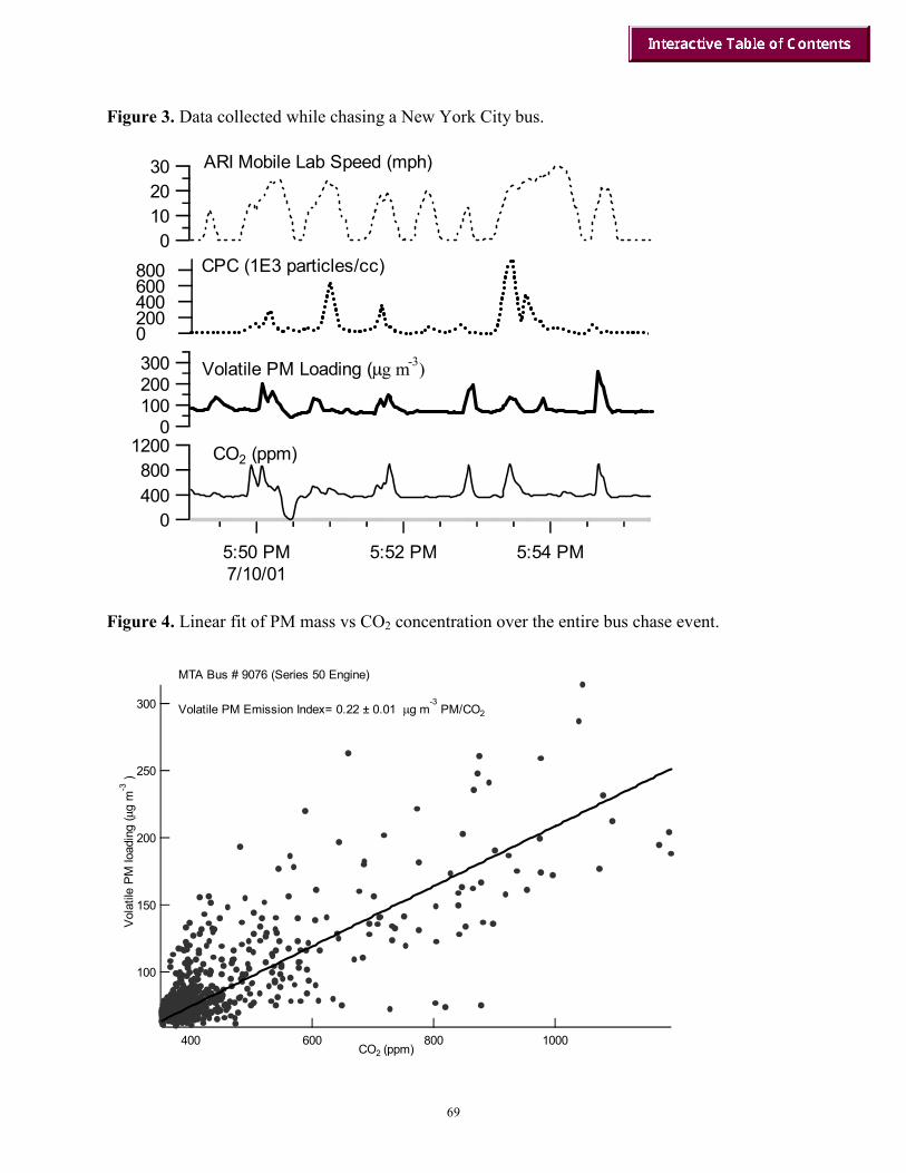
69

Figure 3. Data collected while chasing a New York City bus.

Figure 4. Linear fit of PM mass vs CO2 concentration over the entire bus chase event.

5:50 PM7/10/01

5:52 PM 5:54 PM

1200800400

0

CO2 (ppm)

300200100

0

Volatile PM Loading (µg m-3)

8006004002000

CPC (1E3 particles/cc)

3020100

ARI Mobile Lab Speed (mph)

300

250

200

150

100

Vol

atile

PM

load

ing

(µg

m-3

)

1000800600400CO2 (ppm)

MTA Bus # 9076 (Series 50 Engine) Volatile PM Emission Index= 0.22 ± 0.01 µg m

-3 PM/CO2

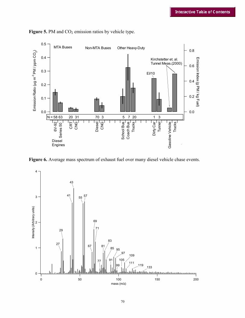
70

Figure 5. PM and CO2 emission ratios by vehicle type.

Figure 6. Average mass spectrum of exhaust fuel over many diesel vehicle chase events.

0.5

0.4

0.3

0.2

0.1

0.0Em

issi

on R

atio

(µg

m-3

PM

/ pp

m C

O2)

6V-9

2S

erie

s 50

C

RT

CN

G D

iese

lC

NG

Sch

ool B

usC

oach

Bus

Truc

ks

D

irty

Car

Tunn

el G

asol

ine

Veh

icle

Truc

ks

0.8

0.6

0.4

0.2

0.0

Em

ission Index (g PM

/ kg Fuel)

58 63 20 31 70 3 5 7 20 1 3

EI/10

MTA Buses Non-MTA Buses Other Heavy-Duty

Diesel Engines

N =

Kirchstetter et. al. Tunnel Meas.(2000)

4

3

2

1

0

Inte

nsity

(Arb

itrar

y un

its)

200150100500mass (m/z)

27

29

41

43

55 57

67

69

71

81

83

85 9597

9977 91 105

109

111119 133

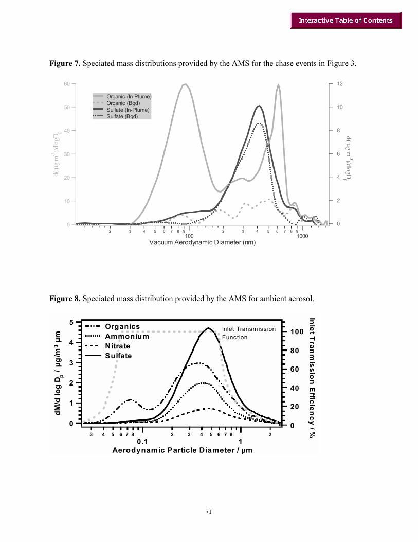
Figure 7. Speciated mass distributions provided by the AMS for the chase events in Figure 3.

Figure 8. Speciated mass distribution provided by the AMS for ambient aerosol.

5

4

3

2

1

0

dM/d

log

D p / µ

g/m

3 µ

m

3 4 5 6 7 80.1

2 3 4 5 6 7 81

2

Aerodynamic Particle Diameter / µm

100

80

60

40

20

0

Inlet Tranmissio

n E

fficiency / %

Organics Ammonium Nitrate Sulfate

Inlet TransmissionFunction

60

50

40

30

20

10

0

d( µ

g m

-3)/d

logD

p

2 3 4 5 6 7 8 9100

2 3 4 5 6 7 8 91000

Vacuum Aerodynamic Diameter (nm)

12

10

8

6

4

2

0

d( µg m-3)/dlogD

p

Organic (In-Plume) Organic (Bgd) Sulfate (In-Plume) Sulfate (Bgd)

On-Line Mass Spectral Analysis of Thermally Evaporated Diesel Exhaust Particles

Paul J. Ziemann and Herbert J. TobiasAir Pollution Research Center, University of California, Riverside, California 92521

Hiromu Sakurai and Peter H. McMurryParticle Technology Laboratory, Department of Mechanical Engineering,

University of Minnesota, Minneapolis, Minnesota 55455

David B. KittelsonCenter for Diesel Research, University of Minnesota, Minneapolis, Minnesota 55455

IntroductionIn this paper, we describe the use of a thermal desorption particle beam mass

spectrometer (TDPBMS) for chemical analysis of the volatile component of diesel particles. Thisinstrument is especially well-suited to this task because the volatile component of particulateengine exhaust (i.e., organics and sulfuric acid) has only a few potential sources. Here, wedescribe two TDPBMS techniques developed for this study which employ mass spectralmatching methods to obtain quantitative information on particle composition: one employs thedistinctive mass spectra of lubricating oil and a synthetic fuel, while the other involves themeasurement of temperature-dependent mass spectra, in order to evaluate the contributions offuel, oil, organic oxidation products, and sulfuric acid to diesel particles. From the results of thisstudy, we then evaluate the potential for using the mass spectra of the volatile component ofambient particles as a signature for diesel particulate matter.

ExperimentalExhaust from a heavy-duty diesel engine operating on an engine dynamometer was

diluted in a two-stage, variable residence time dilution system (Khalek et al., 1999) and thensampled directly into the TDPBMS for particle chemical analysis. In the TDPBMS (Tobias et al.,2000), particles are sampled into aerodynamic lenses and focused into a narrow beam fortransport through two flat-plate skimmers separating three differentially-pumped chambers. Inthe detection chamber (~10-7 torr), they impact in a V-shaped molybdenum foil vaporizer with~40-100% efficiency. The vaporizer is mounted on a copper rod outside the mass spectrometerionizer and the temperature is monitored by an attached thermocouple. Particles are eithercontinuously vaporized for real-time analysis by resistively heating the foil at ~250 oC, or theyare collected for temperature-programmed thermal desorption (TPTD) analysis (Tobias andZiemann, 1999) by cooling the foil to –50 oC using an external liquid nitrogen bath and thenheating at 90 oC/min to desorb components according to volatility. Desorbing molecules areionized by 70 eV electrons and analyzed using a quadrupole mass spectrometer with a pulsecounting detector. The fuels used in this study were California [CA] low-sulfur (96 ppm S),Fischer-Tropsch [FT] (<1 ppm S), and U.S. Environmental Protection Agency [EPA] on-highway (360 ppm S), and the lubricating oil was a commercially available 15W40 oil for dieselengines. Standard particles for TDPBMS analysis were generated by atomizing solutions of CAfuel, FT fuel, and used oil .

74

Results and DiscussionIn this study, TDPBMS analysis focused on determining the relative contributions of fuel,

oil, organic oxidation products, and sulfuric acid to diesel particle composition. The approachused here to interpret TDPBMS mass spectra is the following:

(1) Mass spectra are representative of “volatile” diesel particulate components that evaporate attemperatures less than ~200-400 oC, including organics and sulfuric acid, but “nonvolatiles”such as soot (elemental carbon), metals, or metal oxides are not analyzed.

(2) The major components that can contribute to mass spectra are unburned fuel, unburned oil,oxidized organic combustion products, and sulfuric acid.

(3) Unburned fuel, unburned oil, oxidized organic combustion products, and sulfuric acid havecharacteristic mass spectra that can be used to identify these components by comparison withdiesel particle mass spectra. As shown in Figure 1, CA fuel (Figure 1A) and oil (Figure 1C)have complex spectra with contributions from many compounds, including primarilybranched and cyclic alkanes and aromatics. They also have significant signal at many of thesame masses because they contain the same classes of hydrocarbons. The important featurefor identification purposes is that the relative intensities of many neighboring peaks in thespectra are consistently different between fuel and oil. The mass spectrum of FT fuel (Figure1B), which is a synthetic fuel, is dominated by a series of alkane peaks and is therefore easierto distinguish from oil than CA fuel. Mass spectra of monocarboxylic acids, which are themajor oxidized organic combustion products found in diesel particles by GC-MS analysis,have major peaks at m/z (mass/charge) 60 and 73 (palmitic acid [CH3(CH2)14C(O)OH] isshown in Figure 1D) that can be used as markers for oxidized organic combustion products.The mass spectrum of sulfuric acid has large peaks at m/z 64, 81, and 98 as shown in Figure1E. The m/z 64 peak is not abundant in fuel, oil, or carboxylic acids and therefore serves asan indicator of this compound.

(4) The relative amounts of the major components of diesel particles can be estimated bycomparing diesel particle mass spectra to those created by mixing different fractions ofnormalized, standard component mass spectra. Because the total mass spectral signalobtained from hydrocarbons is proportional to the mass of sample, the component spectra arenormalized by dividing the signal at each mass by the total signal. The standard spectrum thatyields the best match to the particle spectrum is then used to determine the mass fraction ofeach component in the mixture.

Figure 2A shows a real-time mass spectrum of diesel particles sampled with the enginerunning on FT fuel. Note first that the markers for oxidized organic combustion products at m/z60 and 73 (Figure 1D) and for sulfuric acid at m/z 64 (Figure 1E) are very small, indicating thatthese species contribute little to the diesel particle mass. The major components are thereforesome combination of unburned fuel and oil. In Figures 2B-D are shown standard spectra of fueland synthesized fuel:oil mixtures. The diesel particle mass spectrum is clearly different from thatof pure fuel, as indicated by the different patterns and relative intensities in the m/z 67-71 and 81-85 regions, and the m/z 71, 85, 99, …, 183, 197 series of alkyl [CH3(CH2)n

+] fragments that isprominent in fuel but not particles. The mass spectra of particles and standard fuel:oil mixtures

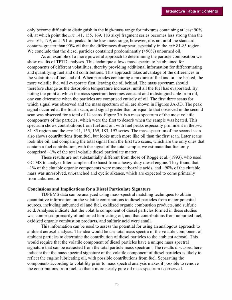
75

only become difficult to distinguish in the high-mass range for mixtures containing at least 90%oil, at which point the m/z 141, 155, 169, 183 alkyl fragment series becomes less strong than them/z 165, 179, and 191 oil peaks. In the low-mass range, however, it is not until the standardcontains greater than 90% oil that the differences disappear, especially in the m/z 81-85 region.We conclude that the diesel particles contained predominantly (>90%) unburned oil.

As an example of a more powerful approach to determining the particle composition weshow results of TPTD analyses. This technique allows mass spectra to be obtained forcomponents of different volatilities, thereby providing additional information for differentiatingand quantifying fuel and oil contributions. This approach takes advantage of the differences inthe volatilities of fuel and oil. When particles containing a mixture of fuel and oil are heated, themore volatile fuel will evaporate first, leaving the oil behind. The mass spectrum shouldtherefore change as the desorption temperature increases, until all the fuel has evaporated. Bynoting the point at which the mass spectrum becomes constant and indistinguishable from oil,one can determine when the particles are comprised entirely of oil. The first three scans forwhich signal was observed and the mass spectrum of oil are shown in Figures 3A-3D. The peaksignal occurred at the fourth scan, and signal greater than or equal to that observed in the secondscan was observed for a total of 14 scans. Figure 3A is a mass spectrum of the most volatilecomponents of the particles, which were the first to desorb when the sample was heated. Thisspectrum shows contributions from fuel and oil, with fuel peaks especially prominent in the m/z81-85 region and the m/z 141, 155, 169, 183, 197 series. The mass spectrum of the second scanalso shows contributions from fuel, but looks much more like oil than the first scan. Later scanslook like oil, and comparing the total signal from the first two scans, which are the only ones thatcontain a fuel contribution, with the signal of the total sample, we estimate that fuel onlycomprised ~1% of the total volatile diesel particulate matter.

These results are not substantially different from those of Rogge et al. (1993), who usedGC-MS to analyze filter samples of exhaust from a heavy-duty diesel engine. They found that~1% of the elutable organic components were monocarboxylic acids, and ~90% of the elutablemass was unresolved, unbranched and cyclic alkanes, which are expected to come primarilyfrom unburned oil.

Conclusions and Implications for a Diesel Particulate SignatureTDPBMS data can be analyzed using mass-spectral matching techniques to obtain

quantitative information on the volatile contributions to diesel particles from major potentialsources, including unburned oil and fuel, oxidized organic combustion products, and sulfuricacid. Analyses indicate that the volatile component of diesel particles formed in these studieswas comprised primarily of unburned lubricating oil, and that contributions from unburned fuel,oxidized organic combustion products, and sulfuric acid were small.

This information can be used to assess the potential for using an analogous approach toambient aerosol analysis. The idea would be use total mass spectra of the volatile component ofambient particles to determine the contribution of diesel particles to the ambient aerosol. Thiswould require that the volatile component of diesel particles have a unique mass spectralsignature that can be extracted from the total particle mass spectrum. The results discussed hereindicate that the mass spectral signature of the volatile component of diesel particles is likely toreflect the engine lubricating oil, with possible contributions from fuel. Separating thecomponents according to volatility prior to mass spectral analysis makes it possible to removethe contributions from fuel, so that a more nearly pure oil mass spectrum is observed.

76

Unfortunately, using this oil signature to identify diesel contributions to ambient aerosol isprobably not possible, since there will be oil emissions from non-diesel vehicles and othercombustion sources. Furthermore, although we have not analyzed a selection of lubricating oils,it is quite possible that they vary in their mass spectral signatures. Nonetheless, it would beuseful to search out data on the mass spectra of various engine lubricating oils and the total massspectra of particles from other combustion sources, specifically those with similar volatility todiesel engine lubricating oils. Particle mass spectrometer data of this type are probably notreadily available (although such measurements could be made), but may not be necessary. Anumber of researchers have used GC-MS for analysis of filter-collected particles from a widearray of combustion sources. Although the focus of these analysis was usually on theidentification and quantification of individual compounds, there may be mass spectra availableon the large, low-volatility, unresolved complex mixture that is typically observed in theseanalyses. This material is usually ignored because it cannot be resolved, but it is the majorcomponent of the particulate organic matter and would contain any unburned diesel oil.

AcknowledgementsWe are grateful to the Coordinating Research Council and the California Air Resources

Board for funding this research, which is co-sponsored by the Engine ManufacturersAssociation, Southcoast Air Quality Management District, Cummins, Caterpillar, and Volvo.

ReferencesKhalek, I.A., Kittelson, D.B., Brear, F., 1999. SAE Technical Paper Series, 1999-01-1142.Rogge, W.F., Hildemann, L.M., Mazurek, M.A., Cass, G.R., Simoneit, B.R.T., 1993. Environ.

Sci. Technol. 27, 636.Tobias, H.J., Ziemann, P.J., 1999. Anal. Chem. 71, 3428.Tobias, H.J., Kooiman, P.M., Docherty, K.S., Ziemann. P.J., 2000. Aerosol Sci. Technol. 33,170.

77

Figure 1. Real-Time TDPBMS mass spectra of (A) CA fuel, (B) FT fuel, (C) used oil, (D)palmitic acid, and (E) sulfuric acid.

60 80 100 120 140 160 1800

20

40

60

80

100

Rel

ativ

e In

tens

ity

m/z200

141

97

111

149

CA Fuel 8571

127

197183169

A

155

60 80 100 120 140 160 1800

20

40

60

80

100

Rel

ativ

e In

tens

ity

m/z200

141

99

113

FT Fuel 8571

127

197183169

B

155

60 80 100 120 140 160 1800

20

40

60

80

100

Rel

ativ

e In

tens

ity

m/z200

137

97

111

Used Oil8169

123

191179

C

149 165141

0

2 0

4 0

6 0

8 0

100

5 0 100 150 200 250

Rel

ativ

e In

tens

ity

m/z

Palmitic AcidC H

3( C H

2)

1 4COOH6 0

7 3

256

129

213

D

60 80 100 120 140 160 1800

20

40

60

80

100

Rel

ativ

e In

tens

ity

m/z200

81

80

Sulfuric Acid98

64

E

78

Figure 2. Real-Time TDPBMS mass spectra of (A) diesel particles obtained from the engineoperating with FT fuel at 20% load and (B-D) synthesized mass spectra obtained by mixingfractions of the real-time TDPBMS mass spectra of FT fuel and used oil.

6 0 8 0 100 120 140 160 1800

2 0

4 0

6 0

8 0

100

Rel

ativ

e In

tens

ity

m/z200

137

9 7111

149

Total Diesel Particles�

8 1

6 9

123

191179165

141

6 0 8 0 100 120 140 160 1800

2 0

4 0

6 0

8 0

100

Rel

ativ

e In

tens

ity

m/z200

9 7

111

50% FT Fuel : 50% Oil7 1

127

197183

141

169

8 5

155

6 0 8 0 100 120 140 160 1800

2 0

4 0

6 0

8 0

100

Rel

ativ

e In

tens

ity

m/z200

141

9 7

111

10% FT Fuel : 90% Oil8 1

6 9

125

191179149 165

8 5

155137

6 0 8 0 100 120 140 160 1800

2 0

4 0

6 0

8 0

100

Rel

ativ

e In

tens

ity

m/z200

137

9 7

111

Used Oil8 16 9

123

191179

149 165141

A

B

C

D

79

Figure 3. Temperature-dependent TPTD mass spectra of diesel particles obtained from theengine operating with CA fuel at 20% load. The first scan in which signal was observed is (A)Scan 1, (B) and (C) are the next scans, and (D) is the mass spectrum of used oil.

6 0 8 0 100 120 140 160 1800.0

1.8 103

3.6 103

5.4 103

7.2 103

9.0 103

Sign

al In

tens

ity (c

ps)

m/z200

137

9 7111

149

Scan 1

8 1

7 1

125

197181

165153

8 5

169141 155

183

6 0 8 0 100 120 140 160 1800.0

1.2 104

2.4 104

3.6 104

4.8 104

6.0 104

Sign

al In

tens

ity (c

ps)

m/z200

139

9 7111

149

Scan 2

6 9

125

191181165

8 3

6 0 8 0 100 120 140 160 1800.0

4.8 104

9.6 104

1.4 105

1.9 105

2.4 105

Sign

al In

tens

ity (c

ps)

m/z200

137

9 7

111

149

Scan 3

6 9125

191179165

8 1

6 0 8 0 100 120 140 160 1800

2 0

4 0

6 0

8 0

100

Rel

ativ

e In

tens

ity

m/z200

137

9 7

109

Used Oil

8 1

6 9

125

191179153 165

D

C

B

A

Figures 1, 2A, 2C, 2D, and 3A–D are reprinted with permission from Sakurai H, Tobias HJ, Park K, Zarling D, Doherty KS, Kittelson DB, McMurry PH, Ziemann PJ. On-line measurements of diesel nanoparticle composition and volatility. Atmos Environ 37:1199-1210.

Using Individual Particle Signatures to DiscriminateBetween HDV and LDV Emissions

Sergio A. Guazzotti and Kimberly A. PratherDepartment of Chemistry and Biochemistry

University of California, San Diego

Introduction

Results from several epidemiological studies have shown a relationship between exposure toPM and increases in mortality and morbidity (e.g., Schwartz, 1991; Dockery et al., 1993; Pope et al.,1995; Vedal, 1997; Zhu et al., 2002; Brunekreef and Holgate, 2002). Emissions of particles frommotor vehicles are one of the major contributors to the concentration of fine particles in theatmosphere (e.g., Finlayson-Pitts and Pitts, 2000), and are considered the most significant source ofultrafine particles in urban environments (Zhu et al., 2002). As indicated in the HEI Research onDiesel Exhaust Program Summary, diesel engines are a significant fraction of the transportation fleetas well as an essential component of the industrial infrastructure (HEI, 1999). Thereforedifferentiation between particulate emissions emitted from gasoline and diesel-powered vehiclescould help in determining the relative contributions of these sources to the ambient aerosol.

Recently, single particle mass spectrometry techniques, such as aerosol time-of-flight massspectrometry (ATOFMS), have been used to characterize particulate emissions from differentcombustion sources including biomass, vehicular, and coal-burning emissions. ATOFMS allows forthe determination of the size and chemical composition of individual particles as they are emitteddirectly from a given source. By carrying out source characterization studies, exclusive combinationsof ion markers are being determined and unique fingerprints are being established. Efforts toapportion particles in the atmosphere from different sources by using combinations of unique singleparticle fingerprints are underway. Such research is vital to understanding the effects of specificsources on health (Laden et al., 2000; Morawska and Zhang, 2002). In addition, single particleanalysis allows monitoring of transformations of the chemical composition of the particles after theyare emitted from the corresponding sources. In this presentation, several source characterizationstudies using the ATOFMS technique are presented. Combinations of single particle mass spectralfingerprints are discussed that allow distinction between HDV and LDV emissions and ultimately theapportionment of particles from these sources in ambient measurements.

Experimental Methods

Aerosol time-of-flight mass spectrometryTransportable aerosol time-of-flight mass spectrometers (ATOFMS) were developed in our

former laboratory at the University of California, Riverside (US Patents 5,681,752 and 5,998,215). Asdescribed in previous publications (Prather, Nordmeyer et al. 1994; Noble and Prather 1996; Gard etal. 1997), ATOFMS allows for characterization of the aerodynamic diameter and chemicalcomposition of individual particles from a polydisperse aerosol in real time. Details on the function ofthe transportable ATOFMS are described elsewhere (Gard et al., 1997). There are a number ofresearch groups working in this area; three recent review articles describe the differences betweensingle particle mass spectrometry techniques (Suess and Prather, 1999; Johnston, 2000; Noble andPrather, 2000).

Briefly, individual aerosol particles are introduced into the instrument, where they areaccelerated through a converging nozzle, achieving different terminal velocities depending on theiraerodynamic diameters. Particles are drawn from atmospheric pressure through a converging nozzleinto an initial vacuum region held at approximately 3 Torr. Due to the pressure differential, the gasundergoes supersonic expansion resulting in smaller particles being accelerated to higher terminalvelocities than larger particles. After this first stage, the aerosol beam passes through two stages ofdifferential pumping separated by skimmers. The collimated particle beam then enters the light-

scattering region, where the transit time for particles traveling between two scattering lasers ismeasured and recorded. Upon instrument calibration, the particle transit time is used to obtain theaerodynamic size of each particle. After exiting the sizing region, the particles immediately enter theion source region of a dual-ion reflectron time-of-flight mass spectrometer. The measured velocity ofthe particle and known distances between lasers are used to fire a frequency-quadrupled Nd:YAGlaser (266 nm) at the exact time the particle arrives in the ion source region, desorbing and ionizingspecies from each sized particle in flight. Typically, the laser has a pulse energy of ~1 mJ, pulse widthof ~7 ns, and spot size of ~0.5 mm, resulting in a power density of approximately 108 Wcm-2.

Positive and negative ions from the particle are simultaneously accelerated in oppositedirections by the ion optics in the ATOFMS and detected using a pair of microchannel plate detectors.Both positive and negative ion time-of-flight mass spectra are then correlated with the aerodynamicdiameter measured for each particle. It is important to note that ATOFMS acquires both positive andnegative ion mass spectra for each particle, providing information on all cations and anions presentsimultaneously. Dual ion measurements are essential for source apportionment of particles as well asdetermining whether the particles have undergone reactions with gas-phase species in the atmosphere(Kane et al., 2002). The transportable ATOFMS instruments are calibrated for aerodynamic size usingpolystyrene latex spheres (PSL, Interfacial Dynamics Corporation) of known aerodynamic diameter.These standardized particles are suspended in water, atomized using a Collison atomizer, dried usingtwo 30-cm diffusion dryers filled with silica gel, and then sent directly into the ATOFMS for sizecalibration.

The ATOFMS instruments currently in use have been modified from the ones described inthe literature to allow for increased dynamic range data acquisition. This modification in the dataacquisition system has the advantage of preventing peaks in the mass spectra of detected particlesfrom being off-scale. This is important for particle analysis, in which the ion signals in each particlemass spectrum can differ by several orders of magnitude. This is achieved by using two identicaldigitizers, one with the input attenuated by 30 dB, connected via a signal splitter to the signal source.The signals from both digitizers (attenuated and nonattenuated) are acquired and recombined in theATOFMS acquisition software (after proper baseline-subtraction and multiplication of the attenuatedsignal by the corresponding attenuation factor). Another instrumental modification that has beenperformed involves the use of a new inlet to focus sampled particles with aerodynamic diametersbetween 0.05 and 0.3 µm into the ATOFMS. The concentrating inlet consists of a series of orificeswith decreasing diameters along the axis of the inlet (Liu et al., 1995a and 1995b), and allows fortransferring particles into a narrow centerline (<1 mm) with close to 100% transmission efficiencyover the desired size range. The integration of this inlet into the ATOFMS system has resulted in animprovement in transmission efficiency of 6 orders of magnitude for particles with aerodynamicdiameter below 0.3 µm (Su et al., manuscript in preparation).

ATOFMS single particle data analysis and quantitationData sets obtained during ambient sampling with ATOFMS instruments are analyzed using

various analytical tools developed in our laboratory over the past 10 years. For example, particles canbe classified into exclusive classes by carrying out searches in a Matlab-based database or in MSAccess, where specified threshold values (ion area, relative ion area, mass/charge ratios, etc.) forspecific ions can be chosen (e.g., Gard et al., 1997; Silva et al., 1999; Liu et al., 2000; Angelino et al.,2001; Guazzotti et al., 2001). Also, automatic sorting and classification of particles with similarspectral characteristics is achieved by using an adaptive resonance theory-based neural networkalgorithm, ART-2a (Song et al., 1999). ART-2a separates particles into distinct classes of chemicallysimilar particles within large ATOFMS data sets and generates new classes whenever a data point(mass spectrum) falls outside a present proximity to all existing classes, therefore having theadvantage of determining contributions from previously detected particle classes while introducinginformation on new particle types. General descriptions of the ART-2a algorithm have been presentedin previous publications (e.g., Carpenter et al., 1991; Xie et al., 1994; Hopke and Song, 1997).

Proper scaling of ATOFMS data to account for differences in transmission efficiencies forparticles of different aerodynamic diameters is typically performed by comparing ATOFMS data withsimultaneously acquired data from colocated instrumentation such as Optical Particle Counters,Aerodynamic Particle Sizers, Scanning Mobility Particle Sizers, and micro-orifice uniform deposit

impactors (MOUDI) (e.g., Hughes et al., 1999; Allen et al., 2000; Guazzotti et al., 2001; Wenzel etal., 2002). Using this scaling method, particle number concentrations for different particle classes areevaluated and compared with other relevant data so accurate concentrations of the various types areobtained. This scaling procedure is extremely important since the ATOFMS with its standard nozzleconfiguration detects larger particles much more efficiently than smaller ones. Also, massconcentration values of size-segregated chemical composition for various elements obtained withMOUDI are compared with those values inferred from ATOFMS single particle analysis, showingexcellent agreement between the techniques (e.g., Fergenson et al., 2001; Guazzotti et al., 2002).

Correlations with semicontinuous techniques are carried out as well. For example,comparison of ATOFMS data with those obtained with an Automated Particle Nitrate (APN) monitor(Stolzenburg and Hering, 2000) has been performed, allowing for evaluation of the temporal variationof the mass concentration of nitrate-containing particles as determined by the ATOFMS and APNsystems, showing good agreement between the two techniques (Liu et al., 2000). Quantification of 44different chemical species from ATOFMS data has been carried out using a multivariate method, two-dimensional partial least squares analysis (Fergenson et al., 2001), showing the applicability of thisroutine, which is less labor-intensive than a univariate approach. Most recently, MOUDI comparisonshave allowed ATOFMS data to be scaled to yield precise mass concentrations of ammonium, nitrate,and sulfate (Bhave et al., 2002). All of these evaluation, calibration, and comparison studies clearlyshow the ability of ATOFMS to produce quantitative information on the concentrations of size-resolved particle classes and chemical species.

Results and Discussion

Source characterization and apportionment using ATOFMS single particle informationA number of single particle studies by ATOFMS have focused on determining distinct

chemical fingerprints from particles emitted from different vehicular sources, i.e., light-duty vehicles(gasoline and diesel-powered vehicles), and heavy-duty vehicles (e.g., Silva and Prather, 1997; Silvaet al., 1999; Gross et al., 2000; Silva et al., 2000; Suess and Prather, 2002; Suess et al., 2002). Theseincluded two tunnel studies (at the Caldecott Tunnel), three dynamometer studies, and one freewaystudy.

Three dynamometer studies have been carried out in which several light-duty gasoline-powered vehicles and diesel-powered vehicles were tested while operating under the Federal TestProcedure (FTP) (Figures 1 and 2). Different vehicular combustion particles were identified, andqualitative ion markers for distinct particle types have been determined. In a recent dynamometerstudy investigating heavy-duty diesel particle emissions, ATOFMS was used to characterize thecomposition of particles emitted under a variety of driving cycles. The effects of various parameterson particle composition including dilution conditions, truck age, and engine type were investigated. Itwas shown that the ATOFMS coupled with the dynamometer/dilution system resulted in highlyreproducible single particle chemical signatures (Suess and Prather, 2002). Figures 3, 4, and 5 showresults from the ART-2a classification of particles emitted from diesel-powered vehicles, withrepresentative mass spectra being presented for the top three clusters (particle classes). From the massspectral information these clusters can be classified as cluster1, particles containing calcium,elemental carbon, and sulfates; cluster 2, particles containing elemental carbon, calcium, and sulfates;and cluster 3, particles containing calcium, nitrates, and phosphates. Using the ATOFMS techniquethe temporal evolution of these particle classes during the FTP cycle could be evaluated, with distinctcontributions during different stages in the cycle being observed (Figure 6). In general, highercontributions of particles containing EC were observed from diesel emissions when compared withgasoline-powered vehicles (for particles with aerodynamic diameters between 0.2 and 2.5 µm).Calcium was, in general, more associated with diesel emissions, whereas vanadium was morefrequently observed in particles emitted from gasoline-powered vehicles.

The studies performed in the Caldecott Tunnel allowed for the determination of differencesbetween single particle signatures from LDV versus HDV, since both LDV and HDV are allowedthrough one bore of the tunnel, whereas only LDV are allowed to pass through a second bore in thesame direction. Single particles were characterized with distinct particle classes observed. Themarkers in these particles were similar to those obtained in several dynamometer studies.

Apportionment of gasoline and diesel particles in ambient aerosol samples has beenperformed taking into consideration ATOFMS results obtained in these studies (Gross et al., 2000;Suess et al., 2002), and applying ART-2a analysis in combination with a multivariate method, partialleast squares analysis (Song et al., 2002). Comparison of single particle signatures observed fromsource characterization studies and ambient studies carried out in Atlanta also have been performed,allowing the evaluation of similarities in observed signatures from ambient particles and those fromdiesel-powered and gasoline-powered vehicles. Finally, it is important to mention that the sourceapportionment accuracy of ART-2a has been tested with synthetic single particle data generated by asource-oriented aerosol processes trajectory model, a model that allows for chemical transformationof particles to take place during transport (Bhave et al., 2001). The strength of single particle analysisusing a technique such as ATOFMS lies in the ability to establish chemical signatures andassociations (fingerprints) that can be used to unequivocally separate particle source contributions inambient air. Being able to perform accurate source apportionment is vital to understanding the role ofaerosols in affecting human health and regional and local climates.

References

Allen, J.O., D.P. Fergenson, E.E. Gard, L.S. Hughes, B.D. Morrical, M.J. Kleeman, D.S. Gross, M.E.Gaelli, K.A. Prather, and G.R. Cass, Particle detection efficiencies of aerosol time of flightmass spectrometers under ambient sampling conditions, Environmental Science &Technology, 34 (1), 211–217, 2000.

Angelino, S., D.T. Suess, and K.A. Prather, Formation of aerosol particles from reactions ofsecondary and tertiary alkylamines: Characterization by aerosol time-of-flight massspectrometry, Environmental Science & Technology, 35 (15), 3130–3138, 2001.

Bhave, P.V., D.P. Fergenson, K.A. Prather, and G.R. Cass, Source apportionment of fine particulatematter by clustering single-particle data: Tests of receptor model accuracy, EnvironmentalScience & Technology, 35 (10), 2060–2072, 2001.

Bhave, P., J.O. Allen, B.D. Morrical, D.P. Fergenson, G.R. Cass, and K.A. Prather, A field-basedapproach for determining ATOFMS instrument sensitivities to NH4

+ and NO3- in size-

segregated atmospheric particles, Environmental Science and Technology, ASAP article,2002.

Brunekreef, B. and S.T. Holgate, Air pollution and health, The Lancet, 360, 1233-1242, 2002.Carpenter, G.A., S. Grossberg, and D.B. Rosen, Art 2-a — An adaptive resonance algorithm for rapid

category learning and recognition, Neural Networks, 4 (4), 493–504, 1991.Dockery, D.W., A. Pope, X. Xu, J.D. Spengler, J.H. Ware, M.E. Fay, B.G. Ferris, F.E. Speizer, An

association between air pollution and mortality in six US cities, New England Journal ofMedicine, 329, 1753–1759, 1993.

Fergenson, D.P., X.H. Song, Z. Ramadan, J.O. Allen, L.S. Hughes, G.R. Cass, P.K. Hopke, and K.A.Prather, Quantification of ATOFMS data by multivariate methods, Analytical Chemistry, 73(15), 3535–3541, 2001.

Finlayson-Pitts, B.J., and J.N. Pitts, Chemistry of the upper and lower atmosphere: Theory,experiments, and applications, Academic Press, 2000.

Gard, E., J.E. Mayer, B.D. Morrical, T. Dienes, D.P. Fergenson, and K.A. Prather, Real-time analysisof individual atmospheric aerosol particles: Design and performance of a portable ATOFMS,Analytical Chemistry, 69 (20), 4083–4091, 1997.

Gross, D.S., M.E. Galli, P.J. Silva, S.H. Wood, D.Y. Liu, and K.A. Prather, Single particlecharacterization of automobile and diesel truck emissions in the Caldecott Tunnel, AerosolScience and Technology, 32 (2), 152–163, 2000.

Guazzotti, S.A., K.R. Coffee, and K.A. Prather, Continuous measurements of size-resolved particlechemistry during INDOEX-intensive field phase 99, Journal of Geophysical Research-Atmospheres, 106 (D22), 28607–28627, 2001.

Guazzotti, S.A., D.T. Suess, K.R. Coffee, K.A. Prather, P.K. Quinn, T.S. Bates, A. Wisthaler, A.Hansel, W. Ball, R.R. Dickerson, C. Neusuess, AND P.J. Crutzen, Characterization OFPollution Outflow From India and Arabia: Biomass Burning and Fossil Fuel Combustion,Submitted to Journal of Geophysical Research-Atmospheres, 2002.

HEI, The Health Effects Institute, Research on Diesel Exhaust Program Summary, Cambridge MA,1999.

Hopke, P.K., and X.H. Song, Classification of single particles by neural networks based on thecomputer-controlled scanning electron microscopy data, Analytica Chimica Acta, 348 (1-3),375–388, 1997.

Hughes, L.S., J.O. Allen, M.J. Kleeman, R.J. Johnson, G.R. Cass, D.S. Gross, E.E. Gard, M.E. Galli,B.D. Morrical, D.P. Fergenson, T. Dienes, C.A. Noble, P.J. Silva, and K.A. Prather, Size andcomposition distribution of atmospheric particles in southern California, EnvironmentalScience & Technology, 33 (20), 3506–3515, 1999.

Johnston, M.V. Sampling and analysis of individual particles by aerosol mass spectrometry, Journalof Mass Spectrometry, 35¸585–595, 2000.

Kane, D.B., J. Wang, K. Frost, M.V. Johnston, Detection of negative ions from individual ultrafineparticles, Analytical Chemistry, 74, 2092–2096, 2002.

Laden, F., L.M. Neas, D.W. Dockery, J. Schwartz, Association of particulate matter from differentsources with daily mortality in six U.S. cities, Environmental Health Perspectives, 108(10),941–955, 2000.

Liu, D.Y., K.A. Prather, and S.V. Hering, Variations in the size and chemical composition of nitrate-containing particles in Riverside, CA, Aerosol Science and Technology, 33 (1-2), 71–86,2000.

Liu, P., P.J. Ziemann, D.B. Kittelson, and P.H. McMurry, Generating particle beams of controlleddimensions and divergence. 1. Theory of particle motion in aerodynamic lenses and nozzleexpansions, Aerosol Science and Technology, 22 (3), 293–313, 1995a.

Liu, P., P.J. Ziemann, D.B. Kittelson, and P.H. McMurry, Generating particle beams of controlleddimensions and divergence. 2. Experimental evaluation of particle motion in aerodynamiclenses and nozzle expansions, Aerosol Science and Technology, 22 (3), 314–324, 1995b.

Morawska, L., J. Zhang, Combustion sources of particles. 1. Health relevance and source signatures,Chemosphere, 49, 1045–1058, 2002.

Noble, C.A., and K.A. Prather, Real-time measurement of correlated size and composition profiles ofindividual atmospheric aerosol particles, Environmental Science & Technology, 30 (9), 2667–2680, 1996.

Noble, C.A. and K.A. Prather, Real-time single particle mass spectrometry: A historical review of aquarter century of the chemical analysis of aerosols, Mass Spectrometry Reviews, 19(4), 248–274, 2000.

Pope, C.A., M.J. Thun, M.M. Namboodiri, D.W. Dockery, J.S. Evans, F.E. Speizer, C.W. Heath Jr.,Particulate pollution as a predictor of mortality in a prospective study of U.S. adults,American Journal of Respiratory and Critical Care Medicine, 151, 669, 1995.

Prather, K.A., T. Nordmeyer, and K. Salt, Real-time characterization of individual aerosol particlesusing time-of-flight mass spectrometry, Analytical Chemistry, 66 (9), 1403–1407, 1994.

Schwartz, J., Air pollution and daily mortality in Philadelphia, Meeting of the American LungAssociation, Anaheim, CA, 1991.

Silva, P.J., and K.A. Prather, On-line characterization of individual particles from automobileemissions, Environmental Science & Technology, 31 (11), 3074–3080, 1997.

Silva, P.J., D.Y. Liu, C.A. Noble, and K.A. Prather, Size and chemical characterization of individualparticles resulting from biomass burning of local southern California species, EnvironmentalScience & Technology, 33 (18), 3068–3076, 1999.

Silva, P.J., R.A. Carlin, and K.A. Prather, Single particle analysis of suspended soil dust fromSouthern California, Atmospheric Environment, 34 (11), 1811–1820, 2000.

Song, X.H., P.K. Hopke, D.P. Fergenson, and K.A. Prather, Classification of single particles analyzedby ATOFMS using an artificial neural network, ART-2A, Analytical Chemistry, 71 (4), 860–865, 1999.

Stolzenburg, M.R., and S.V. Hering, Method for the automated measurement of fine particle nitrate inthe atmosphere, Environmental Science & Technology, 34 (5), 907–914, 2000.

Suess, D. T. and K.A. Prather, Mass spectrometry of aerosols, Chemical Reviews, 99, 3007–3035,1999.

Suess, D. T. and K.A. Prather, Reproducibility of single particle chemical composition during heavyduty diesel truck dynamometer study, Aerosol Science and Technology, 36(12), 1139–1141,2002.

Suess, D.T., D.S. Gross, P.J. Silva, K.A. Prather, J.J. Schauer, G.R. Cass, Single particle types from agasoline and diesel powered vehicular combustion source characterization study, inpreparation, 2002.

Vedal, S., Ambient particles and health: lines that divide, Journal of the Air and Waste ManagementAssociation, 47, 551–581, 1997.

Wenzel, R.J., D.Y. Liu, E. Edgerton, and K.A. Prather, ATOFMS scaling procedures for the AtlantaSupersite experiment: Part 2, accepted for publication in Journal of Geophysical Research-Atmospheres, 2002.

Xie, Y., P.K. Hopke, and D. Wienke, Airborne particle classification with a combination of chemicalcomposition and shape index utilizing an adaptive resonance artificial neural network,Environmental Science & Technology, 28 (11), 1921–1928, 1994.

Zhu, Y., W.C. Hinds, S. Kim, S. Shen, and C. Sioutas, Study of ultrafine particles near a majorhighway with heavy-duty diesel traffic, Atmospheric Environment, 36, 4323–4335, 2002.

Figure 1. Heavy-duty diesel vehicles tested.

Table 1. Truck Descriptions

# Year Type Make1 1985 HDD Tractor International2 1990 HDD Tractor Peterbuilt3 1994 HDD Tractor Freightl iner4 1995 HDD Tractor Freightl iner5 1995 HDD Tanker Freightl iner6 1996 HDD Tractor Kenworth7 1998 HDD Tractor Peterbuilt8 2000 HDD Tractor Navistar International9 2000 HDD Tractor Freightl iner

10 2000 HDD Tractor Freightl iner

GVW (lbs) Miles32000 501,58650000 399,22452000 639,10550000 241,84345000 689,53632000 50785548000 607,96852000 92,36252000 16698135000 17048

Major goals: Test effects of dilution conditions, vehicle, dyno cycles*Also, refuse truck, MDD truck, 2 city buses**With WDR capabilities

HDV Dyno Study (Fall, 2001)

Figure 2. Light-duty vehicles tested.

Cars Light Duty TrucksCategory Year Make Category Year MakeSmoker 1968 Mercury Cougar 3-way cat. 1995 Chevy SuburbanSmoker 1993 Chevy Blazer 3-way cat. 1996 Nissan Pickup

Non-catalyst 1966 Ford Mustang 3-way cat. 1987 Suzuki SamuriNon-catalyst 1953 Chevy Bel-Air 3-way cat. 1989 Toyota SR-5

Oxidation 1980 Honda Accord 3-way cat. 1989 Dodge CaravanOxidation 1979 Toyota Corolla LEV 2000 Toyota TacomaOxidation 1977 Mercedes 280e LEV 2000 Jeep Gd. Cherokee3-way cat. 1998 Ford Mustang LEV 1998 Ford Explorer3-way cat. 1988 Plymoth Horizon LEV 2002 Nissan Pathfinder3-way cat. 1991 Ford Taurus LEV 2003 Chevy Silverado3-way cat. 1991 Toyota Camry3-way cat. 1994 Honda Integra Cycles: FTP, UC, UCC12, UCC503-way cat. 1999 Cadillac DeVille Total: 29 vehicles3-way cat. 1988 Honda Civic

LEV 1996 Honda Civic Size range (50-300 nm: ~40,000 part.)LEV 1998 Honda Accord Size range (0.2-2.5 microns: ~20,000 partLEV 1999 Nissan SentraLEV 2002 Chevy Monte CarloLEV 1999 Toyota Camry

0 10 20 30 40 50 60 70 80 90 1000

0.2

0.4

0.6

0.8

mass/charge

Cluster 1 from dyno3b with 702 members

0 10 20 30 40 50 60 70 80 90 1000

0.1

0.2

0.3

0.4

0.5

mass/charge

Arb

itra

ry I

nte

nsi

ty2

Arb

itra

ry I

nte

nsi

ty+

Figure 3. Mass spectrum representative of particles in cluster 1.


0 10 20 30 40 50 60 70 80 90 1000

0.2

0.4

0.6

0.8

Arb

itrar

y In

tens

ity +

mass/charge

Cluster 2, from dyno3b with 635 members.

0 10 20 30 40 50 60 70 80 90 1000

0.2

0.4

0.6

0.8

mass/charge

Arbi

trary

Inte

nsity

-


0 10 20 30 40 50 60 70 80 90 1000

0.2

0.4

0.6

0.8

Arbi

trary

Inte

nsity

+

mass/charge

Cluster 3, from dyno3b with 376 members.

0 10 20 30 40 50 60 70 80 90 1000

0.1

0.2

0.3

0.4

0.5

mass/charge

Arb

itrar

y In

tens

ity -

Figure 6. Contribution of stages of the FTP cycles to particle clusters.

15:50 16:19 16:48 17:16 17:45 18:140

10

20

30

40

50

60

Time

c1c2c3

Temporal Histogram of c1, c2, and c3

Idle

Creep

Transient

Extended Idle

Ext. Creep

Cruise

Cou

nts

Ca/EC/SO4

EC/Ca/SO4

Ca/NO3/PO4

93

Diesel Exhaust Signatures for Source Attribution: Part 1

James J. Schauer University of Wisconsin–Madison

Diesel particulate matter is a complex mixture of organic compounds, elemental carbon, and other tracer elements. Considerable efforts have been directed at identifying a “tracer” for diesel particulate matter that can be readily measured to help regulators and health scientists understand the concentration of diesel particulate matter in a given atmospheric particulate matter sample. It has been well recognized that the particulate matter from diesel emissions, as well as from emissions from catalyst-equipped gasoline-powered motor vehicles, food-cooking operations, biomass burning, secondary organic aerosol, and cigarette smoke are predominately carbonaceous, and that their trace elemental composition cannot be accurately used to track the emissions back to these sources. In recent years, a variety of studies have used elemental carbon as a tracer for diesel particulate matter in the urban atmosphere. It is important to recognize, however, that there are other important sources of elemental carbon in the atmosphere including gasoline-powered motor vehicles, coal combustion, and wood smoke (Hildemann et al 1991; Watson et al 1998, 2001). Figure 1 shows the contribution of elemental carbon to some of these sources.

A further complication in the use of elemental carbon as a tracer for diesel particulate matter is the fact that there exist different methods for the analysis of elemental carbon, which are not equivalent (Chow et al 1993, 2001; Schauer et al 2003). Figure 2 shows the dependence of the fraction of carbon that is measured as elemental carbon for two different organic and elemental carbon analysis methods. Unfortunately, past integration of EC measurements, which were obtained by different EC analytical techniques, has led to considerable confusion concerning the viability and utility of elemental carbon measurements. A recent elemental carbon interlaboratory comparison study (Schauer et al 2003) demonstrated consistent organic and elemental carbon measurements for a series of ambient and source samples among participants of the ACE-Asia field study when a consistent method for the analysis of elemental carbon was employed. The results of the intercomparison study are significant since they demonstrate that although elemental carbon cannot be used as a unique tracer for diesel particulate matter, elemental carbon measurements are robust and can be used to help in source identification.

Methods developed over the past decade to speciate particle-phase organic compounds present in source emissions and atmospheric samples have provided new opportunities for fingerprinting particulate matter emissions that can be used in source apportionment efforts (Rogge et al 1991, 1993a,b,c,d, 1997a,b, 1998; Schauer et al 1999a,b, 2000, 2001, 2002a,b,c). As a result of these efforts, several approaches could be used that exploit the organic speciation data for source attribution. To this end, it is important to identify the attributes of tracer compounds that will provide a robust methodology for source attribution in the context of diesel particulate matter. Key considerations include:

1. No single tracer can be universally applied to all environments. The use of tracers must be

employed with knowledge of the domain of the receptor site that includes a qualitative understanding of the sources of particulate matter at that location and all of the potential sources of that tracer.

2. Source fingerprints, which are composed of a series of tracers, have higher specificity for

sources than single tracer compounds.

3. The ability to use source fingerprints to accurately apportion source contribution depends on the ability to identify differences in the source profiles that are sufficiently unique in the context of the atmospheric mixture of sources.

94

4. Source tracers that have low specificity need to be used with extreme caution. It is important to recognize that generic combustion species, including elemental carbon and polycyclic aromatic hydrocarbons, come from many sources, and if all sources are not appropriately represented, significant biases will occur in source attribution calculations. In contrast, tracers that have specificity to the source (i.e., molecular markers) are much less prone to interferences from unidentified sources.

5. Source profiles for diesel and gasoline-powered vehicles cannot be derived from factor

analysis tools, since a subset of the diesel fleet follows the same driving patterns as gasoline-powered vehicles. As shown by Ramadan and colleagues (Ramadan et al 2000) factor analysis based tools can be used to separate segments of the motor vehicle fleet, but this approach does not separate the contribution of gasoline-powered motor vehicles and diesel vehicles.

6. Extreme caution is needed in the use of gas-phase tracers to track particulate matter since the

wet and dry deposition rates of gases and particles are not the same.

7. The relative composition of diesel particulate matter is greatly affected by engine operating condition (Kweon et al 2002). There is no generic average composition of diesel particulate matter that can be broadly employed for all environments. Accurate source attribution that seeks to understand the relative contribution of particulate matter from gasoline and diesel-powered engines must employ profiles that reflect average emissions for the specific environments. Specific parameters that affect the emissions profile of motor vehicles include vehicle fleet distribution, driving cycle distribution, cold start, and vehicle fuel.

Schauer and others (Schauer et al 1999b, 2002b) provided a detailed description of the emissions

of gasoline and diesel engines. These results for diesel engines are shown in Figure 3. Although the relative composition of the components identified by Schauer and others (Schauer et al 1999b, 2002b) will vary as a function of the operating conditions discussed above, these species are very characteristic of motor vehicle exhaust. Likewise, there is a clear understanding of which emissions components originated from lube oil, unburned fuel, and pyrolyzed fuel and lube oil. In the context of the criteria listed above, Schauer and colleagues (Schauer et al 1996) used an emissions inventory approach to identify the appropriate tracer species for dominant particulate matter species present in southern California. Due to the fact that primary emissions of carbonaceous aerosols from coal combustion and fuel oil combustion are not major sources of particulate matter in southern California, the tracers identified by Schauer and colleagues ( Schauer et al 1996) should be applied with caution to locations where significant primary emissions of carbonaceous particulate matter exist. In such locations, additional tracers must be employed to properly account for these additional sources.

In several studies in California, where primary emissions of carbonaceous particulate matter from coal and fuel oil combustion were found to be small, contributions to atmospheric concentrations of hopanes and steranes were found to be dominated by the emissions of diesel and gasoline powered engines, and contributions to elemental carbon concentrations were found to be dominated be these same engines plus wood burning (Schauer et al 1996, 2000, 2002a). Figure 4 shows the contributions of sources to these tracers for a study conducted in Bakersfield during a high-pollution episode that was found to have been significantly impacted by wood smoke. Since highly specific tracers for wood burning have been identified (Simoneit 1999; Schauer et al 2001), hopanes, steranes, wood smoke markers, and elemental carbon measurements provide a robust mechanism to track the presence of diesel particulate matter. The ability of these tracers to provide meaningful results, however, still depends on accurate source profiles that provide an accurate representation of the average emissions from these sources. Likewise, it is important to recognize that these source fingerprints will vary as a function of location and season as a result of the factors discussed above.

95

The initial source apportionment studies that used organic compounds as tracers (Schauer et al 1996, 2000, 2002a; Zheng et al 2002) provide a powerful strategy for tracking the contributions of particulate matter in the atmosphere. In order for this strategy to be applied more broadly and to further reduce the uncertainty of such calculations, the following are needed:

1. More source profiling is needed to develop source profiles that represent a larger and more

statistically selected vehicle fleet. Efforts should be focused on both gasoline and diesel-powered vehicles.

2. Efforts need to be directed at understanding the primary engine parameters that affect the

distribution of tracers in motor vehicle exhaust emissions. Due to the cost associated with source characterization and the broad distribution of vehicle fleets, fuels, and engine operating parameters, there is a great need to have predictive capabilities to assess the impact of such changes on emissions. Clearly, more source profiles are needed than are likely to be generated by vehicle dynamometer tests.

3. Source profiles for coal combustion and fuel oil combustion need to be developed to better

understand the impact of these sources and how the presence of emissions from these sources impacts abilities to apportion diesel particulate matter.

4. Methods need to be developed that can greatly reduce the resources and costs associated with

the analysis of organic compounds in particulate matter samples. In addition, efforts need to be directed at reducing the mass of particulate matter needed for organic speciation in particulate matter samples.

5. Larger data sets of measurements of particle-phase organic compounds need to be generated

to allow the application of factor analysis tools to be employed as a consistency check for chemical mass balance models.

References Chow, J. C.; Watson, J. G.; Crow, D.; Lowenthal, D. H.; Merrifield, T. Aerosol Sci. Technol. 2001, 34,

23-34. Chow, J. C.; Watson, J. G.; Pritchett, L. C.; Pierson, W. R.; Frazier, C. A.; Purcell, R. G. Atmospheric

Environment Part a-General Topics 1993, 27, 1185-1201. Hildemann, L. M.; Markowski, G. R.; Cass, G. R. Environ. Sci. Technol. 1991, 25, 744-759. Kweon, C. B.; Foster, D. E.; Schauer, J. J.; Okada, S. SAE 2002, In Press. Ramadan, Z.; Song, X. H.; Hopke, P. K. J. Air Waste Manage. Assoc. 2000, 50, 1308-1320. Rogge, W. F.; Hildemann, L. M.; Mazurek, M. A.; Cass, G. R.; Simoneit, B. R. T. Environ. Sci. Technol.

1998, 32, 13-22. Rogge, W. F.; Hildemann, L. M.; Mazurek, M. A.; Cass, G. R.; Simoneit, B. R. T. Environ. Sci. Technol.

1997a, 31, 2726-2730. Rogge, W. F.; Hildemann, L. M.; Mazurek, M. A.; Cass, G. R.; Simoneit, B. R. T. Environ. Sci. Technol.

1997b, 31, 2731-2737. Rogge, W. F.; Hildemann, L. M.; Mazurek, M. A.; Cass, G. R. Environ. Sci. Technol. 1994, 28, 1375-

1388. Rogge, W. F.; Hildemann, L. M.; Mazurek, M. A.; Cass, G. R.; Simoneit, B. R. T. Environ. Sci. Technol.

1993a, 27, 2700-2711. Rogge, W. F.; Hildemann, L. M.; Mazurek, M. A.; Cass, G. R.; Simoneit, B. R. T. Environ. Sci. Technol.

1993b, 27, 2736-2744.

96

Rogge, W. F.; Hildemann, L. M.; Mazurek, M. A.; Cass, G. R.; Simoneit, B. R. T. Environ. Sci. Technol. 1993c, 27, 1892-1904.

Rogge, W. F.; Hildemann, L. M.; Mazurek, M. A.; Cass, G. R.; Simoneit, B. R. T. Environ. Sci. Technol. 1993d, 27, 636-651.

Rogge, W. F.; Hildemann, L. M.; Mazurek, M. A.; Cass, G. R.; Simonelt, B. R. T. Environ. Sci. Technol. 1991, 25, 1112-1125.

Rogge, W. F.; Mazurek, M. A.; Hildemann, L. M.; Cass, G. R.; Simoneit, B. R. T. Atmospheric Environment Part a-General Topics 1993e, 27, 1309-1330.

Schauer, J. J.; Cass, G. R. Environ. Sci. Technol. 2000, 34, 1821-1832. Schauer, J. J.; Fraser, M. P.; Cass, G. R.; Simoneit, B. R. T. Environ. Sci. Technol. 2002a, In Press. Schauer, J. J.; Kleeman, M. J.; Cass, G. R.; Simoneit, B. R. T. Environ. Sci. Technol. 1999a, 33, 1566-

1577. Schauer, J. J.; Kleeman, M. J.; Cass, G. R.; Simoneit, B. R. T. Environ. Sci. Technol. 1999b, 33, 1578-

1587. Schauer, J. J.; Kleeman, M. J.; Cass, G. R.; Simoneit, B. R. T. Environ. Sci. Technol. 2001, 35, 1716-

1728. Schauer, J. J.; Kleeman, M. J.; Cass, G. R.; Simoneit, B. R. T. Environ. Sci. Technol. 2002b, 36, 1169-

1180. Schauer, J. J.; Kleeman, M. J.; Cass, G. R.; Simoneit, B. R. T. Environ. Sci. Technol. 2002c, 36, 567-575. Schauer, J. J.; Mader, B. T.; DeMinter, J. T.; Heidemann, G.; Bae, M. S.; Seinfeld, J. H.; Flagan, R. C.;

Bertram, T.; Howell, S.; Kline, J. T.; Quinn, P. K.; Bates, T.; Turpin, B. J.; Lim, H. J.; Yu, J. Z.; Yang, H.; Heyword, M. D. Environ. Sci. Technol. 2003, 37,993–1001.

Schauer, J. J.; Rogge, W. F.; Hildemann, L. M.; Mazurek, M. A.; Cass, G. R. Atmos. Environ. 1996, 30, 3837-3855.

Simoneit, B. R. T. Environ. Sci. Pollut. Res. 1999, 6, 159-169. Watson, J. G.; Chow, J. C.; Houck, J. E. Chemosphere 2001, 43, 1141-1151 Watson, J. G.; Fujita, E. M.; Chow, J. C.; Zielinska, B.; Richards, L. W.; Neff, W. D.; Dietrich, D.

"Northern Front Range Air Quality Study (NFRAQS) Final Report, Chapter 4," DRI, 1998. Zheng, M.; Cass, G. R.; Schauer, J. J.; Edgerton, E. S. Environ. Sci. Technol. 2002, 36, 2361-2371.

Figure 1. Reprinted with permission from Schauer et al. 2003 © American Chemical Society. Figure 2. Reprinted with permission from Hildemann et al. 1991 © American Chemical Society.

98

Figure 3. Reprinted with permission from Schauer et al. 1999b © American Chemical Society.

99

Figure 4. Reprinted with permission from Schauer and Cass 2000 © American Chemical Society.

101

Diesel Exhaust Signatures for Source Attribution: Part 2

James J. Schauer University of Wisconsin–Madison

Previous studies have demonstrated that in locations where primary carbonaceous particulate matter emissions from coal combustion and fuel oil combustion are minor sources of atmospheric particulate matter, contributions to atmospheric concentrations of hopanes and steranes are dominated by internal combustion engines. The structures of hopanes and steranes are shown in Figure 1 along with those of other molecular markers that have been used for source identification. In these environments, elemental carbon concentrations are typically dominated by these same internal combustion engines and biomass burning. Under these circumstances, the predominant factor affecting the ability to accurately apportion the contribution of diesel engine emissions on particulate matter concentrations is the ability to accurately represent the average spark ignition (gasoline-powered) vehicle emissions and the average compression ignition (diesel-powered) vehicle emissions. Inaccuracies in these profiles will translate into biases in the split between the estimated contributions from gasoline-powered motor vehicles and diesel vehicles but will not have a significant impact on the estimated source contribution from other sources. This is due to the fact that the estimates for source contributions from non–motor vehicle sources and internal combustion engines are very different. As presented by Schauer and Cass (2000), the source contributions from wood smoke are determined by specific wood smoke markers, which also provide the contribution of wood smoke to the elemental carbon concentrations. The remainder of the elemental carbon and the hopanes and steranes are used to quantify the contributions of gasoline-powered engines and diesel-powered engines by exploiting the difference in the ratios of hopanes plus steranes to elemental carbon between diesel engine exhaust and gasoline engine exhaust. It is important to recognize that these calculations are sensitive to the organic and elemental carbon analysis technique (Schauer et al 2003) and have been specifically developed with the use of the method described by Birch and Cary (1996).

Although significant efforts have been directed at understanding the split between gasoline and diesel engine emissions, it is important to recognize that the difficulty in separating spark ignition and compression ignition engine emissions is due to the similarities in their chemical compositions. The carbonaceous particulate matter emissions from internal combustion engines are basically composed of unburned lubricating oil, the heavy components of unburned fuel, and pyrolyzed fuel and lubricating oil. Because the lubricating oils for compression emissions and spark ignition vehicles are very similar and the chemical natures of pyrolized organic materials are very similar (i.e., elemental carbon), the constituents that make up diesel particulate matter and emissions from gasoline-powered motor vehicles are very similar. The major difference between the particulate matter emissions from these two types of engines is the average relative distribution of the constituents. With this said, however, the emissions of a diesel engine that is emitting high organic carbon (i.e., under idling or cold start conditions) can have a chemical composition more similar to the emissions of a smoking gasoline-powered engine than a diesel engine operating under high load. This is due to the fact that the emissions from the diesel vehicle emitting high organic carbon and the smoking gasoline engine are typically dominated by lubricating oil emissions (Schauer et al 2002). In contrast, the emissions of the diesel engine operating at high load are dominated by pyrolyzed material (i.e., elemental carbon). This raises a question as to the importance of understanding the relative contribution of emissions from the two types of engines.

It is plausible that exposures to specific components of emissions (i.e., unburned lubricating oil, pyrolized material, or engine wear) from diesel engines and gasoline-powered engines have similar health impacts. To this end, efforts to understand the impact of emissions from motor vehicles may be better directed at understanding the contribution of unburned lubricating oil and pyrolyzed fuel or lubricating oil in the atmosphere. Although this strategy has implications for the regulatory process, it is important to recognize that this apportionment strategy can be implemented with a much higher level of certainty than

102

the apportionment of diesel engine and gasoline engine emissions. This results from the fact that the hopanes and steranes (in the absence of primary carbonaceous aerosol emissions from fuel oil combustion and coal combustion) are excellent tracers for unburned lubricating oil in the atmosphere. Likewise, after correcting for the contribution of biomass aerosol to elemental carbon concentrations, the residual elemental carbon concentration is an excellent tracer for “elemental carbon” from motor vehicles. In the presence of fuel oil combustion and coal combustion, additional tracer species can be used to understand the contribution of these sources to the atmospheric concentrations of hopanes and steranes, as well as elemental carbon. Although this apportionment strategy deviates from the traditional approach to understating the impact of source emissions on air quality and human health, if such a strategy can lead to better control strategies and ultimately can better protect human health, then this new paradigm should be pursued. References Birch, M. E.; Cary, R. A. Aerosol Sci. Technol. 1996, 25, 221-241. Schauer, J. J.; Cass, G. R. Environ. Sci. Technol. 2000, 34, 1821-1832. Schauer, J. J.; Kleeman, M. J.; Cass, G. R.; Simoneit, B. R. T. Environ. Sci. Technol. 2002, 36, 1169-

1180. Schauer, J. J.; Mader, B. T.; DeMinter, J. T.; Heidemann, G.; Bae, M. S.; Seinfeld, J. H.; Flagan, R. C.;

Bertram, T.; Howell, S.; Kline, J. T.; Quinn, P. K.; Bates, T.; Turpin, B. J.; Lim, H. J.; Yu, J. Z.; Yang, H.; Heyword, M. D. Environ. Sci. Technol. 2003, In Press.

Figure 1. Examples of Molecular Markers

HOH

H

H

Cholestanol

H

OOHO

HO

OH

LevoglucosanO

OH

Pimaric Acid

RHopanes R

Steranes

Picene

103

Chemical Characterization of On-Road Motor Vehicle PM Emissions

Eric Fujita and Barbara Zielinska Division of Atmospheric Sciences, Desert Research Institute,

University and Community College System of Nevada, Reno, Nevada

HEI has identified development of a signature for diesel exhaust as an important short-term research need to improve exposure assessments in both prospective and retrospective epidemiology studies. The emission rate and chemical composition of gaseous and particulate pollutants from diesel and gasoline vehicles depend upon many factors, which include vehicle age and mileage, fuel, lubricating oil, emission control technology, vehicle operating mode (cold start, hot stabilized), load, ambient temperature, and state of maintenance. The Desert Research Institute has participated in several relevant studies during the past five years. They include the Northern Front Range Air Quality Study (NFRAQS) (Watson et al., 1998; Fujita et al., 1998; Zielinska et al., 2002), the Comparative Toxicity Study (Zielinska and Sagebiel, 2001), the Characterization of PM Emissions from DoD Sources (Zielinska et al., 2002), and the EC Diesel Fuel Emission Characterization Study (Lev-On et al., 2002 ). Ongoing studies include the Gas/Diesel Split Study and Heavy-Duty Vehicle Chassis Dynamometer Testing for Emission Inventory, Air Quality Modeling, Source Apportionment, and Air Toxic Inventory (CRC E-55). These studies are expected to significantly expand the available information on the source signature of motor vehicle exhaust. The following summary describes relevant findings from our previous studies, our ongoing work, and questions that need to be addressed in future work.

Elemental Carbon as a Marker for Diesel Exhaust

Organic carbon and elemental carbon are the most abundant species in motor vehicle exhaust, accounting for over 95% of the total PM mass. The relative abundances of organic and elemental carbon can be quite variable in motor vehicle exhaust profiles. Elemental carbon is dominant in diesel exhaust, but is lower in newer-technology diesel engines. The relative abundance of EC is generally less at lower engine loads. While most gasoline vehicles are relatively clean, especially in hot-stabilized mode, high emitters can have particulate emission rates that are comparable to or exceed those of most diesel vehicles (Figure 1). We have found that gasoline vehicles emit relatively higher amounts of elemental carbon during cold starts and during high accelerations. Gasoline exhaust measured during the NFRAQS (Watson et al., 1998) had an average split of 75% organic carbon and 25% elemental carbon with higher relative EC during cold starts (based on TOR/IMPROVE carbon measurements). Because of the variability of OC/EC splits, gasoline and diesel vehicles cannot be apportioned by carbon analysis alone, and EC is not a unique tracer for diesel exhaust.

Hopanes and Steranes as Markers for Motor Vehicle Exhaust

Hopanes and steranes are present in lubricating oil, with similar compositions for gasoline and diesel vehicles, but are not present in gasoline or diesel fuels (Figure 2). Emission rates of hopanes and steranes are the highest for both gasoline and diesel “high-emitting” vehicles. While hopanes and steranes are useful markers for motor vehicle emission, they cannot be used to distinguish gasoline and diesel exhaust.

Polycyclic Aromatic Hydrocarbons in Motor Vehicle Exhaust

Polycyclic aromatic hydrocarbons (PAHs) are present in emissions from all combustion sources, and the relative proportions of different PAH compounds in emissions from a given source may vary over

104

several orders of magnitude. PAHs exhibit a wide range of volatility, with naphthalene existing almost entirely in the gas phase, while BaP, other five-ring PAHs, and higher-ring PAHs are predominantly adsorbed on particles. The intermediate three- and four-ring PAHs (semivolatile PAHs) are distributed between the two phases. Data from NFRAQS (Figure 3) and the NREL Comparative Toxicity Study (Figure 4) (Zielinska and Sagebiel, 2001) show that gasoline vehicles emit certain PAHs in greater relative abundance to other PAHs than do diesel vehicles. Gasoline vehicles, whether low or high emitters, emit greater amounts of high molecular weight particulate PAHs (e.g., benzo(b+j+k)fluoranthene, benzo(ghi)perylene, ideno(1,2,3-cd)pyrene, and coronene). Figure 5 shows that these PAHs are found in used gasoline motor oil (but not in fresh oil and not in diesel engine oil). The oil acting as a scrubber to remove combustion-produced PAH may explain this. Diesel vehicles also emit particulate PAHs, but in lower relative proportions to other PAHs, especially the semivolatile methylated PAHs. Diesel emissions contained higher proportions of dimethylnaphthalenes, methyl- and dimethylphenanthrenes, and methylfluorenes. These compounds are distributed between the gas and particle phase and thus require backup traps to be quantitatively collected.

Current Study

The Desert Research Institute and University of Wisconsin–Madison are currently conducting a DOE/NREL-sponsored study to apportion the contributions of tailpipe emissions from gasoline-powered and diesel-powered motor vehicles to ambient concentrations of PM2.5 in the South Coast Air Basin (SoCAB). This study is designed to address the range of uncertainties that may be associated with the methods and procedures for sample collection, chemical analysis, and source apportionment. The study calls for DRI and UWM to work cooperatively on sample collection and quality assurance aspects of the project, but to work independently, at least initially, on chemical analysis and data analysis. DRI is using sample collection and analysis methods and CMB procedures that are consistent with those employed in the Northern Front Range Air Quality Study (NFRAQS), and UWM is adhering to methods and procedures used in PM apportionment studies in the Los Angeles area by the California Institute of Technology. As part of the NREL gas/diesel split study, the Environmental Protection Agency and Clean Air Vehicle Technology Center (CAVTC) conducted dynamometer tests during summer 2001 for 57 light-duty SI and two light-duty CI vehicles and West Virginia University (WVU) tested 30 medium-duty and heavy-duty diesel trucks and two diesel buses. Samples were collected during these tests by DRI and UWM for speciation of particulate matter and semivolatile organic compounds (SVOCs). DRI also monitored PM mass and elemental carbon continuously during the dynamometer tests to examine changes in emission rates and ratios of black carbon to PM with varying operating conditions. Other chemical characterizations include fuel and lube oil from the test vehicles and local road dust samples. DRI and UWM also collected daily 24-hour ambient PM and SVOC samples at downtown Los Angeles and Azusa over a period of one month. Additional ambient samples were collected from a mobile van along roadway loops and locations with varying amounts of SI and CI vehicle traffic, and emissions from wood combustion (from a wildfire and campfires at the RV park) and meat cooking (grilled hamburgers at the RV park). Continuous measurements were also made in the mobile laboratory to relate real-time variations in concentrations of black carbon and total particulate to varying traffic conditions, and mix of traffic.

Questions for Further Work

1. What similarities and differences in chemical composition exist between ambient PM2.5 and SVOC samples collected in the South Coast Air Basin and those collected in other urban areas?

2. What are the direct contributions of SI and CI vehicle exhaust and other major source categories to ambient PM2.5 in the other urban areas, and how do the source attributions and associated

105

uncertainties differ in summer and winter and differ from results obtained for the South Coast Air Basin? Based upon receptor modeling performance parameters, are the source composition profiles developed in the gas/diesel split study from SI and CI vehicles in the South Coast Air Basin suitable for apportioning the contributions of SI and CI vehicles to ambient PM in the other cities?

3. What differences exist in the apportionment of PM2.5 samples collected along major roadways versus samples collected at regional air monitoring sites during weekday and weekends? Are these differences consistent with spatial gradients in the relative concentrations of black carbon, PM1.0, CO, and NO?

4. How much of the particulate carbon is explained by direct emissions from motor vehicles and other major sources of particulate carbon? Are the unexplained fractions greater during summer, and are these fractions correlated with oxidation products that are associated with secondary organic aerosols?

5. What differences exist in the relative ambient concentrations of particulate organic carbon and elemental carbon, and total PM2.5 along major roadways versus samples collected at regional air monitoring sites? How do the OC thermograms and OC/EC ratios of fresh on-road emissions differ from downwind regional samples? How do the results vary by measurement method (e.g., TOR versus TOT methods and IMPROVE versus NIOSH protocols)?

6. With appropriate considerations for spatial and temporal (diurnal and day-of-the-week) variations in actual emissions, how well do the source contribution estimates from receptor modeling compare with corresponding source contributions derived from local emissions inventory data?

7. Are the relative ambient concentrations of PM2.5, NOx, CO, and VOCs along roadways and at air monitoring sites consistent with corresponding ratios derived from emission inventory data?

References Fujita, E., J.G. Watson, J.C. Chow, N. Robinson, L. Richards, and N. Kumar (1998). Northern Front

Range Air Quality Study. Volume C: Source Apportionment and Simulation Methods and Evaluation. Final report prepared for Colorado State University, Fort Collins, CO, June 30, 1998.

Lev-On, M., C. LeTavec, J. Uihlein, K. Kimura, T. L. Alleman, D. R. Lawson, K. Vertin, G. J. Thompson, N. Clark, M. Gautam, S. Wayne, R. Okamoto, P. Rieger, G. Yee, B. Zielinska, J. Sagebiel, S. Chatterjeee, K. Hallstrom (2002). Chemical Speciation of Exhaust Emissions from Trucks and Buses Fueled on Ultra-Low Sulfur Diesel and CNG. SAE Technical Paper 2002-01-0432.

Watson, J., E. Fujita, J.C. Chow, B. Zielinska, L. Richards, W. Neff, and D. Dietrich (1998). Northern Front Range Air Quality Study. Final report prepared for Colorado State University, Fort Collins, CO, June 30, 1998.

Zielinska, B., J. McDonald, T. Hayes, J.C. Chow, E.M. Fujita, and J.G. Watson (1998). “Northern Front Range Air Quality Study, Volume B: Source Measurements.” DRI Document No. 6580-685-8750.3F2, prepared for Colorado State University, Fort Collins, CO, and Electric Power Research Institute, Palo Alto, CA, by Desert Research Institute, Reno, NV.

Zielinska, B. and J.C. Sagebiel (2001) Collection of In-Use Mobile Source Emissions Samples for Toxicity Testing, Project # RCI-8-18148-01, Final Report prepared for DoD/NREL, February 2001.

Zielinska, B., J. Sagebiel, C.F. Rogers, W. P. Arnott, K.E. Kelly, D.A. Wagner, J. S. Lighty, A.F. Sarofim, and G. Palmer (2003), Phase and Size Distribution of Polycyclic Aromatic Hydrocarbons in Diesel Vehicle Emissions, in preparation.

Figure 1. Speciated PM2.5 emission rates for LD and HD diesel (top panel) and gasoline (bottom panel) vehicles measured on a dynamometer during the Northern Front Range Air Quality Study (Watson et al, 1998). Speciated data are composites of several vehicles by emission rate (L=low, ML=medium low, M=medium, H=high, and S=smoker) and for Phases 1 (P1) and 2 (P2) of the Federal Test Procedure.

0

1000

2000

3000

D1P

1

D2P

1

D3P

1

D4P

1

D5P

1

D1P

2

D2P

2

D3P

2

D4P

2

D5P

2

HD

D2

HD

D5

HD

D6

HD

D7

HD

D8

HD

D10

HD

D12

HD

D13

HD

D14

HD

D15

HD

D16

HD

D17

HD

D18

HD

D24

HD

D32

Em

issi

ons

(mg/

mile

)PAH_g

hop&ster

PAH_p

NH4

SO4

NO3

Cl

elements

EC

OC_adj

0

250

500

750

1000

L1P1

L2P1

ML1

P1

ML2

P1

M1P

1

M2P

1

M3P

1

H1P

1

H2P

1

L1P2

L2P2

ML1

P2

ML2

P2

M1P

2

M2P

2

M3P

2

H1P

2

H2P

2

S1P1

S1P2

S2P1

S2P2

S3P1

S3P2

Em

issi

ons

(mg/

mile

)

PAH_g

hop&ster

PAH_p

NH4

SO4

NO3

Cl

elements

EC

OC_adj

106

107

Figure 2. Speciated hopanes and steranes in gasoline fuel (gf), diesel fuel (df), gasoline vehicle lube oil (go), and diesel vehicle lube oil (do) for average gasoline or diesel vehicles (av), gasoline vehicle black smoker (blsm), new technology gasoline vehicle (ulev), diesel high PM emitter (hiem), new technology diesel vehicle (nt) (Zielinska and Sagebiel, 2001).

Hopanes

0500

10001500200025003000

35004000

df,a

v

gf,a

v

df,h

iem

gf,b

lsm df,n

t

gf,u

lev

do,a

v

go,a

v

do,h

iem

go,b

lsm

do,n

t

go,u

lev

ug/g

hop9hop27hop26hop25hop24hop23hop22hop21hop20hop19hop18hop17hop16hop15hop14hop13hop12hop11hop10

Steranes

0200400600800

10001200140016001800

df,a

v

gf,a

v

df,h

iem

gf,b

lsm

df,n

t

gf,u

lev

do,a

v

go,a

v

do,h

iem

go,b

lsm do,n

t

go,u

lev

ug/g

ster53ster52ster51ster50ster49ster48_41ster47ster46ster45_40ster44ster43ster42ster39ster38ster37ster36ster35

108

Figure 3. Emission rates of gas-phase PAH (upper panel) and semivolatile and particulate PAH (lower panel) for LD and HD diesel (right panel) and gasoline (left panel) vehicles measured on a dynamometer during the Northern Front Range Air Quality Study (Watson et al., 1998, Zielinska et al., 1998). Speciated data are composites of several vehicles by emission rate (L=low, ML=medium low, M=medium, H=high, and S=smoker) and for Phases 1 (P1) and 2 (P2) of the Federal Test Procedure.

Heavy-Duty Diesel Vehicles

0

10

20

30

40

50

60

HDD2

HDD5

HDD6

HDD7

HDD8

HDD10

HDD12

HDD13

HDD14

HDD15

HDD16

HDD17

HDD18

HDD24

HDD32

naphth mnaph2 mnaph1 dmn267 dm1367 d14523 dmn12 dmn18 biphen m_2bph m_3bph m_4bph

atmnap em_12n btmnap ctmnap em_21n etmnap ftmnap gtmnap htmnap tm128n acnapy acnape

Light-Duty Gasoline Vehicles

0

10

20

30

40

50

60

Low Cold

Low Hot

Low Comp

Med Cold

Med Hot

Med Comp

High Cold

High Hot

High Comp

Su

m o

f PA

H (m

g/m

i)

Heavy-Duty Diesel Vehicles

0

1

2

3

4

5

6

7

HDD2

HDD5

HDD6

HDD7

HDD8

HDD10

HDD12

HDD13

HDD14

HDD15

HDD16

HDD17

HDD18

HDD24

HDD32

phenan fluore a_mflu m_1flu b_mflu c_mflu a_mpht m_2pht b_mpht c_mpht m_1phtdm36ph a_dmph b_dmph c_dmph dm17ph d_dmph e_dmph anthra m_9ant fluora pyrenea_mpyr b_mpyr c_mpyr d_mpyr e_mpyr f_mpyr retene bntiop baanth m_7baa chrysnbbjkfl bepyrn bapyrn m_7bpy incdpy dbanth bbchrn bghipe corone

Light-Duty Gasoline Vehicles

0

1

2

3

4

5

6

7

Low Cold

Low Hot

Low Com

p

Med Cold

Med Hot

Med Com

p

High Cold

High Hot

High Com

p

Su

m o

f PA

H (m

g/m

i)

109

Figure 4. Speciated PAH concentrations in gasoline exhaust (upper panel) and diesel exhaust (lower panel) (Zielinska et al., 2003). Gasoline vehicle exhaust contains higher relative abundances of high molecular weight particulate PAHs than does diesel exhaust. The reverse applies to methylated PAHs.

Gasoline, Load, Filter

0102030405060708090

phen

an

mef

lu

xano

ne

mep

hen

dmep

hen

anth

ra

fluor

a

pyre

ne

bntio

p

mef

l/py

bzcp

hen

baan

th

chry

sn

bbjk

fl

bepy

rn

bapy

rn

incd

py

bghi

pe

dban

th

coro

ne

ng/m

3

Diesel, High Load, Filter

0

500

1000

1500

2000

2500

3000

phen

an

mef

lu

xano

ne

mep

hen

dmep

hen

anth

ra

fluor

a

pyre

ne

bntio

p

mef

l/py

bzcp

hen

baan

th

chry

sn

bbjk

fl

bepy

rn

bapy

rn

incd

py

bghi

pe

dban

th

coro

ne

ng/m

3

Denuded Filter Undenuded Filter

Diesel, High Load, Filter

0

20

40

60

80

100

chry

sn

bbjk

fl

bepy

rn

bapy

rn

incd

py

bghi

pe

dban

th

coro

ne

ng/m

3

110

Figure 5. Speciated PAHs in gasoline fuel (gf), diesel fuel (df), gasoline vehicle lube oil (go), and diesel vehicle lube oil (do) for average gasoline or diesel vehicles (av), gasoline vehicle black smoker (blsm), new technology gasoline vehicle (ulev), diesel high PM emitter (hiem), new technology diesel vehicle (nt) (Zielinska and Sagebiel, 2001).

Oil, Particle PAH

0

100

200

300

400

do,a

v

do,h

iem

do,n

t

go,a

v

go,b

lsm

go,u

lev

ug/g

coronedbanthbghipeincdpybapyrnbepyrnm_7bpybbjkflchry56mchrysn

baanthbzcphen

Fuel, Particle PAH

0

4

8

12

16df

,av

df,h

iem

df,n

t

gf,a

v

gf,b

lsm

gf,u

lev

ug/g

coronedbanthbghipeincdpybapyrnbepyrnm_7bpybbjkflchry56mchrysnbaanthbzcphen

111

A Brief Summary of DOE’s Gasoline/Diesel PM Split Study1

Douglas R. Lawson National Renewable Energy Laboratory, Golden, Colorado 80401

The overall objective of the Gasoline/Diesel PM Split Study, which began in the summer of 2001, is to quantify the relative contributions of tailpipe emissions from gasoline-powered motor vehicles and diesel-powered motor vehicles to ambient concentrations of fine particulate matter (PM2.5) in the urbanized region of Southern California using an organic compound-based chemical mass balance (CMB) model. A fundamental goal of this study is to obtain a better understanding of the uncertainties associated with the CMB receptor modeling approach. This study is necessary, particularly in light of conclusions regarding the relative contributions of diesel and gasoline combustion to ambient concentrations of fine particles from studies in the Los Angeles area (Schauer et al., 1996) and the Northern Front Range of Colorado (Watson et al., 1998; Fujita et al., 1998). These studies are referred to below as the CalTech study and the Northern Front Range Air Quality Study (NFRAQS), respectively.

Several groups will work cooperatively on sample collection and quality assurance aspects of the study, but independently, at least initially, on chemical and data analysis. One group will use sample collection analysis methods and CMB procedures that are consistent with those employed in the CalTech study, and the second group will adhere to methods and procedures used in the NFRAQS. Source and ambient samples must be collected in a manner that can support these independent receptor-modeling calculations. The final result of the following tasks is to separately quantify the primary source contributions of both gasoline-powered vehicles and diesel-powered vehicles and uncertainties associated with these apportionments. It is the responsibility of the investigators to assure that the individual tasks of the project are implemented and integrated in a manner to meet this overall objective. The efforts should build on the efforts previously reported by Schauer et al. (1996) and Fujita et al. (1998). In addition, recommendations outlined by White and Gunst (2000), funded under separate subcontracts by NREL and the Coordinating Research Council, should be properly addressed.

Task 1: Source Testing

The U.S. Environmental Protection Agency (EPA) with the Clean Air Vehicle Technology Center (CAVTC), and West Virginia University (WVU), under separate subcontracts with DOE and NREL, will operate gasoline-powered motor vehicles and diesel-powered motor vehicles, respectively, on their transportable dynamometers at a location in the Los Angeles area. The U.S. EPA with the assistance of the California Bureau of Automotive Repair and the South Coast Air Quality Management District, and WVU will recruit vehicles, drive the vehicles over specified test cycles, and operate their primary dilution tunnels during the testing operations. The investigators will supply a secondary dilution sampler capable of collecting diluted exhaust samples from the primary dilution tunnels of each group’s transportable

1 Summarized from:“Gasoline/Diesel PM Split Study: Source and Ambient Sampling, Chemical Analysis, and Apportionment Phase — Program Plan,” July 25, 2001 by E.M. Fujita, P. Arnott, B. Zielinska, J.C. Sagebiel, D. Campbell, H. Moosmüller, J.C. Chow (Desert Research Institute), J. J. Schauer (University of Wisconsin–Madison), N.N. Clark, S. Wayne (West Virginia University), P.A. Gabele (US Environmental Protection Agency), W. Crews (Clean Air Vehicle Technology Center), D. Saito, C. Stover (California Bureau of Automotive Repair), M. Nazemi (South Coast Air Quality Management District), and other Study documents. NREL Subcontract Nos. ACL-131046-01 and ACL-1-31046-02. Prepared for the National Renewable Energy Laboratory; funding provided by U.S. Department of Energy's Office of Heavy Vehicle Technologies, James Eberhardt, Office Director.

112

dynamometer. The two dynamometers will operate at different times, such that simultaneous operations of different secondary dilution samplers are not required. Sixty gasoline-powered motor vehicles will be tested on the EPA transportable dynamometer using a modified Unified Driving Cycle composed of three phases, with an optional fourth phase that will be added on selected vehicles (Table 1). Separate samples are to be collected for each phase of each vehicle. Including ten percent test repeats and blank tests, 246 sets of samples will be collected for the gasoline-powered motor vehicles. In addition, 126 diesel vehicle tests will be conducted on 32 vehicles (Table 2). Exhaust samples from each diesel vehicle source test will not be divided into separate phases for sample collection. To this end, a total of 372 sets of source samples will be collected. The required samples to be collected for each source test are listed in Table 3.

The second-stage dilution sampler should be operated in a manner consistent with the overall objective of the study to assure that suitable source samples are collected. The researchers are responsible for cleaning and operating the sampler in a manner consistent with the needs of the project. They will also be responsible for providing and preparation of the sampling equipment and sampling substrates required for the collection of the samples listed in Table 3. In addition to the motor vehicle exhaust samples listed above, ten road dust samples should be collected at locations within the urbanized region of Southern California that will be best suited for the source apportionment effort. The road dust samples will be resuspended by the investigators under laboratory conditions to obtain samples compatible with the samples listed in Table 1 that can be analyzed by the same techniques that will be employed for the exhaust and ambient samples.

Task 2: Ambient Sampling Ambient samples are to be collected using ambient samplers that parallel the source samples specified in Tables 1-3. Samples will be collected on the schedule and at the locations given in Table 4. Task 3: Continuous Measurements of Fine Particulate Mass and “Elemental” Carbon

In addition to the substrate-based samples that are to be collected during the source tests, real-time monitors for the measurement of fine particle mass and fine particle “elemental” carbon are to be supplied and operated by the investigators. They will provide estimates of cumulative particulate mass loading for each of the samples collected for subsequent chemical analysis at the conclusion of each run.

The researchers also will install and operate a real-time monitor for measurement of fine particulate “elemental” carbon in the sampling van described in Task 1. They will collect data during times corresponding to the 28 source-dominated ambient samples. Task 4: Chemical Analysis

Measurement of fine particle mass, water-soluble ions by ion chromatography (IC), and trace metals by X-ray fluorescence (XRF) should use methods specified by the EPA Fine Particle Chemical Speciation Network. “Elemental” carbon (EC) and “organic” carbon (OC) are to be measured using four parallel protocols: (1) the IMPROVE temperature/oxygen cycle using the TOR instrument, (2) the NIOSH 5040 temperature/oxygen cycle using the TOR instrument, (3) the IMPROVE temperature/oxygen cycle using the Sunset Labs Instrument, and (4) the NIOSH 504 temperature/oxygen cycle using the Sunset Labs Instrument. Any one method can be used for the analysis of denuded filter samples, but a consistent method must be used throughout all of the denuded samples. Unless noted otherwise in Table 1, each sample collected for mass, water sample ions, trace metals, and EC/OC should be analyzed separately (i.e., no compositing).

Samples for organic compound speciation will be composited to obtain 82 gasoline-powered motor vehicle exhaust samples, 63 diesel exhaust samples, 10 road dust samples, and 43 ambient samples. The compositing schedule was decided collectively by the investigators and NREL after reviewing the

113

mass and EC/OC data for all of the sample sets. A list of the measurements and samples collected for the entire study is given in Table 5. Task 4: Data Analysis and CMB Source Apportionment Modeling Analysis of continuous PM and EC data

The continuous particulate measurements from both the ambient and the source measurements will be made available promptly for the relevant personnel attached to the project. The data will be provided in individual files pertaining to a given day of measurement in the case of ambient sampling, or to a particular vehicle in the case of source sampling. The data will be calibrated to an agreed upon standard of pressure and temperature. In the case of source sampling, the data will be processed and interpolated as appropriate to provide a real-time assessment of the elemental carbon and total carbon content. The data will also be time averaged and accumulated over the entire sampling period and will be compared with filter-based measurements.

1. Instrument comparison for particulate emissions. From dynamometer tests; PM mass versus TEOM, EC/TC by [Photoacoustic (PA)/(TEOM and DustTrak)] versus EC/TC by TOR and TOT. Compare ambient EC by PA with EC by TOR and TOT. 2. Analysis of PM mass, OC/TC, and EC/TC by mode (phase, speed, and acceleration) and

vehicle emitter type.

Evaluation and characterization of source composition profiles The source profiles will be weight fractions of total reconstructed mass with one-sigma analytical

errors for individual measurements. The uncertainties in the composite profiles are the larger of either the one-sigma variations in fractional species abundance among members of the composite or the root mean square of the individual analytical uncertainties. Prior to the actual CMB calculations, initial CMB runs will be performed to select a default combination of source profiles and fitting species. A preliminary set of source profiles consisting of at least one source profile from each of the major source categories will be applied to test ambient samples. Characterization of ambient and emission inventory data

DRI and UWM will summarize the ambient data collected in the field study, along with source data collected at different sampling sites described in the statement of work and quantify associated uncertainties. CMB receptor modeling and emission inventory reconciliation

DRI and UWM will apply the CMB receptor model to the source and ambient data collected during the study and assess the relative importance of gasoline and diesel engine emissions for the sampling locations and times studied in this project. References Fujita, E., J.G. Watson, J.C. Chow, N. Robinson, L. Richards, and N. Kumar (1998). Northern Front

Range Air Quality Study. Volume C: Source Apportionment and Simulation Methods and Evaluation. Final report prepared for Colorado State University, Fort Collins, CO, June 30, 1998.

Schauer, JJ, W.F. Rogge, L.M. Hildemann, M.A. Mazurek, G.R. Cass, B.R.T. Simoneit, (1996). “Source apportionment of airborne particulate matter using organic compounds as tracers.” Atmos. Environ., 30, 3837-3855.

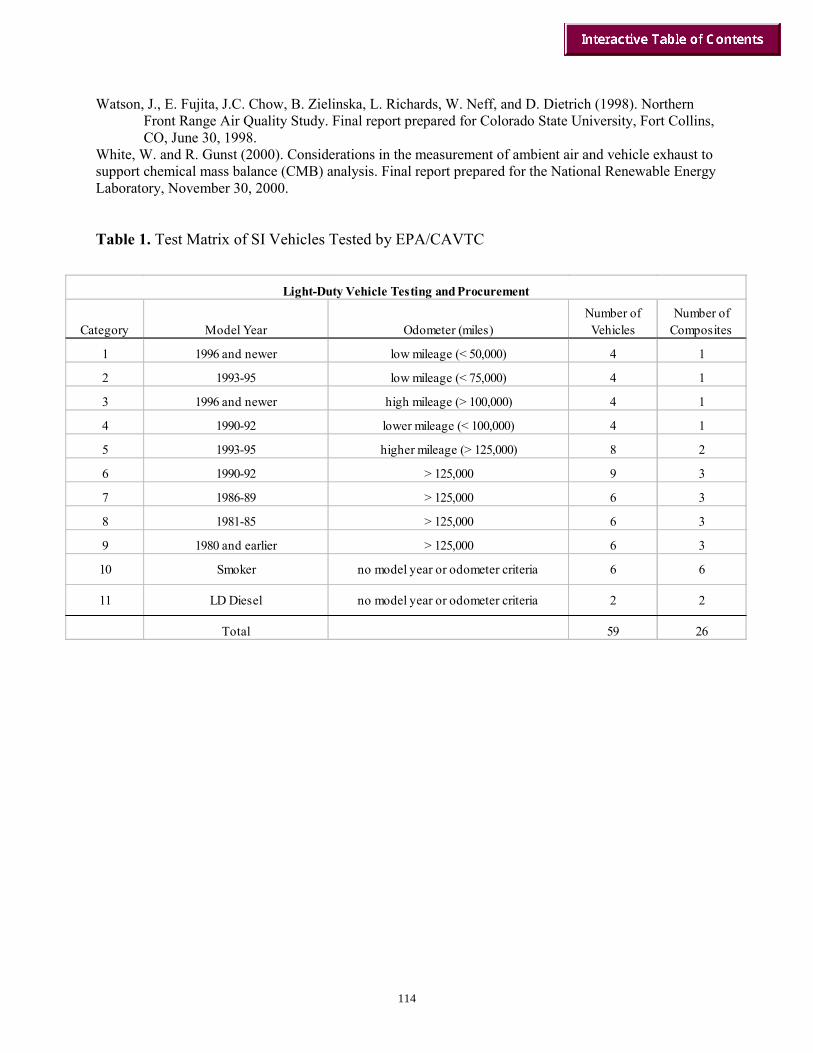
114

Watson, J., E. Fujita, J.C. Chow, B. Zielinska, L. Richards, W. Neff, and D. Dietrich (1998). Northern Front Range Air Quality Study. Final report prepared for Colorado State University, Fort Collins, CO, June 30, 1998.

White, W. and R. Gunst (2000). Considerations in the measurement of ambient air and vehicle exhaust to support chemical mass balance (CMB) analysis. Final report prepared for the National Renewable Energy Laboratory, November 30, 2000.

Table 1. Test Matrix of SI Vehicles Tested by EPA/CAVTC

Light-Duty Vehicle Testing and Procurement

Category Model Year Odometer (miles)Number of Vehicles

Number of Composites

1 1996 and newer low mileage (< 50,000) 4 1

2 1993-95 low mileage (< 75,000) 4 1

3 1996 and newer high mileage (> 100,000) 4 1

4 1990-92 lower mileage (< 100,000) 4 1

5 1993-95 higher mileage (> 125,000) 8 2

6 1990-92 > 125,000 9 3

7 1986-89 > 125,000 6 3

8 1981-85 > 125,000 6 3

9 1980 and earlier > 125,000 6 3

10 Smoker no model year or odometer criteria 6 6

11 LD Diesel no model year or odometer criteria 2 2

Total 59 26

115

Table 2. Test Matrix of CI Vehicles Tested by WVU

GVW (lbs.) Pre 90 90-93 94-97 98-current Total BOX 1 BOX 2 BOX 3 BOX 4

Total 1 Total 1 Total 2 Total 4 8 (C) [1] (C) [2] (B) [3] (D) [5]

(C) [4] (C) [6] (C) [7]

8501 – 14000 (C) [34]

BOX 5 BOX 6 BOX 7 BOX 8 Total 2 Total 0 Total 3 Total 3 8 (C) [8] (B) [10] (D) [13] (C) [9] (C) [11] (B) [14]

14001 – 33000 (C) [12] (C) [15]

BOX 9 BOX 10 BOX 11 BOX 12 Total 2 Total 3 Total 6 Total 5 16 (B) [16] (B) [18] (C) [21] (E) [26] (E) [17] (C) [19] (C) [22] (B) [27]

(C) [20] (C) [23] (C) [28] (C) [24] (C) [29] (C) [25] (C) [30]

33001 – 80000 (C) [33] Total 5 4 11 12 32

Transit Buses

One Powered By Electronic Controlled Diesel - (A) [32] One Powered By Manual Controlled Diesel - (A) [31] Notes: Letters in ( ) are Set ID. Numbers in [ ] are Vehicle Number.

Cycle Set:

(A) CSHVR + Manhattan + Idle

(B) Cold CSHVR + CSHVR + Highway +Idle

(C) CSHVR + Highway +Idle

(D) Cold CSHVR + Highway + Idle + Repeat CSHVRs

(E) Cold CSHVR w/engine brake + CSHVR + Highway + Idle + Cold Idle + UDDS

+ CSHVR w/engine brake

116

Table 3. Fine Particle Sample for Collection for Off-line Analysis During Each Source Test Period

Sample

No. Sample Type

Substrate

Flowrate(lpm)

Intended Analysis

1 Exhaust Teflon Membrane 10 Mass, Elements, and Ions 2 Exhaust Teflon Membrane 10 Mass, Elements, and Ions 3 Exhaust Quartz Fiber 10 EC/OC (Methods 1 and 2)* 4 Exhaust Quartz Fiber 10 EC/OC (Methods 3 and 4)* 5 Exhaust Denuder/Quartz Fiber 10 EC/OC 6 Exhaust Teflon/Denuder/Quartz Fiber 10 EC/OC 7 Exhaust TIGF PUF/XAD 80-120 Organic Compound Speciation 8 Exhaust Quartz Fiber/PUF 80-120 Organic Compound Speciation 9 Dilution

Air Teflon 10 Mass, Water Soluble Ions by

IC≈, and Trace Metals by XRF≈ 10 Dilution

Air Quartz Fiber 10 EC/OC and Organic Compound

Speciation♦ Notes: * See Task 4: Chemical Analysis for details ≈ Half of the samples for IC analysis and half of the samples for X-ray fluorescence (XRF) analysis

♦ Composites of selected samples for organic compound speciation

117

Table 4. Ambient Sampling Plan

118

Table 4. Ambient Sampling Plan (cont.)

119

Table 5. Summary of Measurements and Sample Collection for the Gasoline/Diesel Split Study

121

Particulate Matter from Gasoline Engines

Chad R. Bailey, Carl R. Fulper, Richard W. Baldauf, and Joseph H. Somers US Environmental Protection Agency, Ann Arbor, MI

Mobile Source Emission Models and PM Emission Inventories: Nonroad & On-road, Gasoline & Diesel Mobile source emission inventories for particulate matter (PM) include both on-road and nonroad sources. On-road sources include automobiles, light-duty gasoline trucks, light-duty diesel trucks, heavy-duty gasoline trucks, and heavy-duty diesel trucks. Nonroad sources include the following general categories: Recreational vehicles Construction equipment Industrial equipment Farm/agricultural equipment Light commercial equipment Logging equipment Airport service equipment Each of these categories includes a number of subcategories; the total number of subcategories is about 80. Also, each category includes — to varying degrees — 2-stroke gasoline engines, 4-stroke gasoline engines, and diesel engines for a total of about 240 equipment categories. Also, other nonroad equipment includes aircraft emissions (from both piston and gas turbine aircraft), locomotive engines (all diesel), and commercial marine vessels (which are mostly diesel). The EPA on-road models (MOBILE6, MOBILE6.1, and MOBILE6.2) produce emission factors (e.g., grams emitted per mile of travel) for a fleet average for each of the on-road categories. The fleet average includes emissions for vehicles from the past 25 years weighted by vehicle population estimates. The g/mile emission factors are then coupled with vehicle-miles-traveled data to calculate a total inventory. These data are produced by a variety of transportation agencies, including the U.S. Department of Transportation, state agencies, and metropolitan planning organizations. In the current models, emission factors are estimated for exhaust and tire/brake wear but not, at present, high emitters. The EPA nonroad emission model (NONROAD) is based on g/BHP-hr (grams per brake-horsepower hour) emission factors, which are comparable to fuel or energy-specific emission rates. These are coupled with hours of usage and brake-horsepower hour level of the engine (plus a load factor which accounts for how much of the engine’s available power is used). Also, the model includes total equipment population and estimates of engine activity. The end calculation of the model is the total metric tons for each of the approximately 240 equipment types. Commercial marine, locomotive, and aircraft emissions are calculated by a different methodology and are not, at present, in the nonroad model. These calculations account for emission factors and usage plus the equipment population. In EPA’s National Emission Trends inventory, total yearly mass emissions estimates are developed at the county level for each of approximately 3000 counties in the country. They are also generally developed for each month of the year. Emission inventories are also calculated for a wide variety of stationary sources. These emission inventories serve as the basis for tracking federal progress in air pollution and for conducting regulatory analyses. States and local governments collaborate in developing their own inventories for use in State Implementation Plans to determine how much reduction is needed in various sources. These agencies make use of a wide variety of methods, with differing degrees of sophistication. EPA established guidance for state bodies for the preparation of inventories. It is important that the mobile source emission

122

inventories be accurate to assure that the correct sources are addressed and, also, that needed regulation can be proposed for mobile sources in an accurate manner. EPA’s national emission inventories for the year 2000 show that diesel vehicle/engine emissions dominate the mobile source inventory. In PM, nonroad diesel PM2.5 represents 61% of mobile source PM2.5 emission while on-road diesels represent 29%.

The truck fleet has been subject to federal emissions regulations since the early 1980s. EPA has implemented regulations for new engines built in and after model year 1988. These regulations were made significantly stricter for model years 1991 and 1994. EPA recently finalized a rule that will ensure even greater reductions in PM2.5 emission rates in the 2007 model year, and following. At that point, PM2.5 emissions will be controlled well over 90% (e.g., roughly 99%) compared to emissions from a noncontrol engine. There has been relatively little regulation for nonroad diesel engines, although EPA plans to propose regulations shortly. Thus, it is not surprising that nonroad diesels represent a larger fraction of the PM2.5 inventory than on-road diesels. In the EPA’s Trends inventory, on-road gasoline PM2.5 represents only 12% of primary mobile source PM emissions with primary nonroad gasoline PM representing 17% of PM2.5. Figure 1 shows these contributions. On a national basis, mobile source PM2.5 is currently responsible for about 20% of total PM2.5 in the emission inventories from all sources excluding natural and miscellaneous sources (such as earth crustal material). Several substantial effects are unquantified in EPA on-road emission models. The EPA emission factor models do not at present include high emitters for either on-road or nonroad vehicles/engines. That is, a single emission factor is used in the models which is representative of typical emitters. High emitters can result from normal deterioration as well as malmaintenance. High emitters represent only a small fraction of the vehicles although the g/mile or g/BHP-hr emission factor is considerably higher than that of normal emitters. An additional uncertainty is the lack of estimation of emissions effects from certain driving conditions (high accelerations and heavy-load conditions). They also do not incorporate the effect of lower temperatures. The EPA test procedure for PM is conducted at ambient temperatures of 75o F. Lower temperatures generally result in increased PM emissions. Also, the effect of fuel composition (such as the use of oxygenated compounds in gasoline) is not considered. If high emitters and other conditions were considered, the total amount of PM2.5 from mobile sources would increase beyond the approximately 20% in current national inventories. Also, the relative distribution of diesel and gasoline PM2.5 may change.

The bottom line is that the EPA mobile source PM2.5 emission models used to develop emission inventories must be as accurate as possible. Emission inventories are needed by states to prepare a State Implementation Plan. They are also used in making decisions on what new regulations are needed for PM2.5 such as additional mobile source controls. At present, EPA is undertaking several efforts to improve emission factor models. Ambient PM 2.5 and Receptor Modeling

When state and local agencies prepare State Implementation Plans, they also conduct air quality modeling to predict ambient PM2.5 levels. Air quality modeling for PM accounts for secondary formation of PM. Secondary PM forms from sulfur oxides (for which power plants are a major source), converting to sulfate and nitrogen oxides (for which mobile sources are major contributors), converting to nitrate. The role of organics in forming secondary PM is not entirely clear, although a number of studies recently published have indicated that secondary organic aerosols may be a substantial contributor to overall PM mass in some areas (Strader et al 1999; Brown et al 2002).

Also, a number of air quality monitoring networks measure the amount and composition of PM2.5 in both urban and rural areas. Urban PM2.5 levels and composition shown in Figure 2 are based on data

123

from the EPA Speciation Network in 2001. These data show the importance of carbonaceous PM, which includes both organic and elemental carbon. Rural PM2.5 levels are shown in Figure 3 based on data from the IMPROVE network in 1999. These data also show that carbonaceous PM is an important contributor to total PM but somewhat less so than in urban areas. Also, the levels of PM2.5 are, as expected, lower in the rural areas. Figure 4 shows the excess level and its composition for PM2.5 in urban areas compared to a local rural area. It is clear that both nitrates and carbonaceous PM contribute to this excess. Mobile sources are major contributors to carbonaceous PM2.5.

Also, ambient PM2.5 samples are used in source apportionment studies that analyze ambient PM2.5 and compare its detailed chemical characteristics to the composition of the sources contributing to the PM2.5. These approaches are generally referred to as “chemical mass balance.” Other receptor modeling approaches make use of multivariate statistics to ascertain sources and their ambient mass contributions based on the internal organization of data. Included among these approaches are principal components analysis, factor analyses, and the recently developed “Positive Matrix Factorization” and UNMIX (Paatero and Tapper, 1994; Henry 1997). Both chemical mass balance and multivariate approaches can be applied to ambient monitoring data to ascertain information about sources of PM2.5. Examining the contribution of mobile sources, PM2.5 source apportionment studies using the EPA Chemical Mass Balance (CMB) model have come to different conclusions regarding the contribution to ambient PM2.5 mass from gasoline and diesel exhaust (Watson et al 1998; Zheng et al 2002). The National Renewable Energy Laboratory with Department of Energy funding is sponsoring a study in Los Angeles with Desert Research Institute and Jamie Schauer to see if these investigators, who found differing results in different areas, can reach similar conclusions in applying their methods to the same area (Los Angeles ambient PM2.5). The methods employed by these studies warrant further scrutiny. The CMB model requires the user to define a set of “fitting species” and the concentration of each of these in ambient and source samples (“profiles”). The exclusion of any major sources of the fitting species that are linearly independent of sources that are included in the model can lead to incorrect apportionment of mass by CMB. Different research groups have employed different fitting species in defining source profiles. In recent years, extractable organics have become the basis for much CMB-related research. Just as it is important to consider high emitters for on-road gasoline, on-road diesels, nonroad gasoline, and nonroad diesels, it is important to be sure that adequate mobile source signatures are developed to reflect these four categories. One group of species used to define source profiles in some studies is the polycyclic aromatic hydrocarbons (PAHs). PAHs are present in combustion products, and are characterized by relatively refractory properties that allow them to survive the combustion process, as demonstrated in radiotracer studies. PAH-based CMB studies examining gasoline and diesel separately have employed sampling of on-highway diesel and gasoline vehicles to represent exhaust profiles from all mobile sources. However, different mobile sources may be subject to different uses, and furthermore, may be powered by fuels of varying quality and composition. Several recent studies of highway diesel vehicles have shown that the composition of diesel exhaust varies by driving mode. While diesel exhaust is traditionally thought to be primarily composed of elemental carbon, Ayala and coworkers (2002) recently observed greater than a 50% mass fraction of elemental carbon in idling engines. Similarly, earlier studies have shown a high abundance of elemental carbon in gasoline vehicles under cold-starting conditions. As a result, single modes of operation may be inadequate for the characterization of emissions from mobile sources. Nonroad engines, such as bulldozers, may be engaged in conditions that maximize the load on the engine. It is unclear whether the same engine operated under highway truck driving conditions will adequately represent such engine operations. Of greater relevance to CMB is the exclusion of engines operating on different fuels from highway vehicles. Many two-stroke engines burn a combination of gasoline and motor oil. The exhaust from these engines may be similar in composition to that from a malfunctioning gasoline vehicle, although whether the relative enrichment of oil products in these engines is adequately represented by the variance in the source profiles used in CMB modeling is unclear.

124

Diesel engine applications other than highway use, such as agricultural combines or trains, may use high sulfur diesel fuel. While current highway diesel fuel is limited to 500 ppm sulfur by EPA regulations, off-road diesel fuel sulfur levels are unregulated, and can reach several thousand ppm by concentration. Certain refining processes are used to remove sulfur and produce higher quality fuel for highway use, including hydrotreatment and hydrocracking. Another function of these technologies is the reduction of PAHs in diesel fuel. Being relatively refractory, PAHs do not deliver good combustion performance in engines. Different catalyst formulations can result in different rates of reaction for desulfurization and saturation of PAHs. However, several studies of petroleum manufacturing processes have indicated that the saturation of PAHs is not uniform across species. Chishti and Williams (1999) observed that as hydrotreatment of an unrefined petroleum stock became more severe, the concentration of 3-ring and 4-ring PAHs increased, while 2-ring PAHs were reduced. While this study was conducted on shale oil, diesel desulfurization is subject to similar chemistry. If the preponderance of PAHs in diesel exhaust originate in fuel, as researchers at the University of Leeds have illustrated using isotopic tracers, the relative mass fractions of higher and lower-ring PAHs may differ substantially between engines using on-highway and nonroad fuel.

Some studies have indicated that such PAH profile differences may bear out in emission results. In a presentation at the 2002 Diesel Engine Emissions Reduction Conference, Gautam and colleagues (2002) of West Virginia University illustrated data showing that when a California bus switched from California highway diesel fuel to ultra-low-sulfur fuel, 3-ring and 4-ring PAHs decreased, while 2-ring PAHs increased in concentration in exhaust PM. The inference that may be drawn from this study is that reduced sulfur diesel fuel altered the mass fraction of different PAHs. In the Northern Front Range Air Quality Study, the diesel mass apportionment was most sensitive to 1-methylphenanthrene and dimethylphenanthrenes. In the region of the country in which Denver is located, approximately half the diesel fuel is hydrotreated, while half is not. If the variance assigned to mass profiles employed therein is substantially greater than the change in PAH concentrations from different fuels, then the diesel profiles should be sufficiently representative of nonroad diesel engine exhaust. However, if the fuel differences result in a linearly independent source being excluded or poorly represented by source profiles, then the mass apportionment may be incorrect. However, insufficient characterization of nonroad sources has been conducted to allow for such an evaluation at this time. It is unclear which other organics may be subject to similar concerns. However, such considerations merit caution in the addition of large numbers of organic species to CMB analyses of ambient data. Careful consideration of whether the a priori selection of sources for speciation merits the use of a large number of analytes as fitting species. Multivariate statistical approaches do not suffer from the same concerns, but the lack of speciation of ambient monitors precludes carbonaceous source profiles derived therein from being interpreted as strictly diesel or gasoline exhaust. A number of studies employing the PMF and UNMIX receptor models have used elemental carbon and organic carbon determined by two different thermogravimetric methods as the basis of determining source identity. However, as noted above, elemental and organic carbon are not selective markers of diesel and gasoline exhaust. Furthermore, the 24-hour sampling time of the monitors that have been analyzed thus far implies that source identification is problematic. Several publications have indicated that secondary organic aerosol (SOA) can form in laboratory experiments on gasoline exhaust, specifically via the toluene oxidation pathway. If during a 24-hour sample a large amount of primary particulate and photooxidation-derived SOA are emitted concurrently, the use of elemental and organic carbon will preclude identification of sources definitively. In particular, methods based on the singular value decomposition, such as principal components analysis, will be unable to distinguish these sources. The addition of good “tracer species” to ambient monitors and exposure studies will assist in the identification of sources. Some investigators have used gas species such as carbon monoxide and ozone to identify gasoline engine exhaust and secondary PM, respectively. Signature organic species or ratios of organic species will also be of assistance.

125

Receptor models play an important role in identifying some of the potential sources of PM2.5 and, to a degree, identifying source contributions. However, it should be recognized that inventories and receptor models answer fundamentally different questions. While inventories are region-specific, receptor models need to also consider regional transport of PM2.5 and precursor species from regions far from the study domain. Receptor models provide a valuable insight into certain air quality questions. However, substantial limitations still exist in their implementation for distinguishing gasoline and diesel exhaust. As a result, EPA is undertaking new research to ensure that inventories answer many of the questions raised by receptor modeling studies. High-Emitting On-Road Gasoline Vehicles A joint project is being implemented with the following organizations to investigate the fleet emissions of gasoline PM from light-duty passenger cars and light-duty gasoline trucks. Light-duty gasoline trucks are defined as trucks below 8500 lb gross vehicle weight (the typical pick-up truck). A number of projects in the past have measured emissions from about 400-500 vehicles. However, these vehicles were not chosen from the fleet at random, so the data cannot be used as an emission distribution representative of the fleet as a whole. The largest project is one done by the Coordinating Research Council in Riverside, CA and San Antonio, TX testing about 200 vehicles. Also, the Coordinating Research Council participated in a project with the Northern Front Range Air Quality Study to test about 250 vehicles. These test programs show what are defined as “normal” vehicle emitters to emit about 0.004-0.06 g/mile PM, while what are defined as high emitters emit about 0.4 g/mile, with smokers emitting somewhat over 1 g/mile PM. By contrast, a new vehicle designed to meet current emission standards emits about 0.001 g/mile PM.

Again, these data cannot be used to define the emission distribution in the fleet because the vehicles were not randomly selected. The following organizations plan to join in a project to test about 500 randomly selected light-duty gasoline vehicles in an area of the country (tentatively Kansas City) not subject to a vehicle inspection/maintenance program for emissions: EPA Office of Transportation and Air Quality EPA Emission Inventory Improvement Program EPA Office of Research and Development Department of Energy/National Renewable Energy Lab Coordinating Research Council University of Kansas Department of Transportation Various state/local pollution control agencies Tentative funding level for the entire project might be about $2,000,000. The results from this project will be used to update the EPA emission factor model for PM, MOBILE6.1. In the longer term, the results will also be used in developing a more advanced EPA mobile source emission factor model, MOVES. Initial results should be available in late 2003 with MOBILE6.1 to be revised sometime afterwards. The end result of this work is that the total contribution to PM2.5 from light-duty gasoline vehicles will increase. This contribution will be a larger share of the emission inventory.

126

High-Emitting On-Road Diesel Trucks A number of organizations listed below are engaged in a project to test about 75 heavy-duty diesel trucks in California: California Air Resources Board Coordinating Research Council Department of Energy/National Renewable Energy Laboratory Engine Manufacturers Association South Coast Air Quality Management District Environmental Protection Agency About 75 in-use diesel trucks representative of the in-use fleet in California will be tested. To date, about 25 of these trucks have already been tested. Conclusion There is a major disagreement between emission inventories for PM and some source apportionment studies. There is also disagreement among source apportionment studies on the relative magnitude of gasoline and diesel PM. Since emission inventories are used in programs to decide what PM control is needed, it is important that they be as accurate as possible and, when the data are available, account for high emitters. References Ayala, A.; Kado, N.; Okamoto, R.; Gebel, M.; Rieger, P. (2002) ARB’s Study of Emissions from Diesel

and CNG Heavy-duty Transit Buses. http://www.arb.ca.gov/research/cng-diesel/DEER2002-ARB.pdf.

Brown, S.G.; Herckes, P.; Ashbaugh, L.; et al. (2002) Characterization of organic aerosol in Big Bend National Park, Texas. Atm Env 36:5807–5818.

Chisti, H.M.; Williams, P.T. (1999) Aromatic and hetero-aromatic compositional changes during catalytic hydrotreatment of shale oil. Fuel 78:1805–1815.

Gautam, M.; Wayne, S.; Thompson, G.; Clark, N.; Lyons, D.; Carder, D.; Mehta, S.; Riddle, W. (2002) Concentrations and Size Distributions of Particulate Matter Emissions from Catalyzed Trap-Equipped Heavy-duty Diesel Vehicles Operating on Ultra-low Sulfur EC-D Fuel. http://www.orau.gov/deer2002/Session4/guatam.pdf.

Henry, R. C. (1997) History and fundamentals of multivariate air quality receptor models. Chemometrics Intel Lab Sys 37:525–530.

Paatero, P. and Tapper, U. (1994) Positive Matrix Factorization - a nonnegative factor model with optimal utlization of error-estimates of data values. Environmentrics 5:111–126.

Strader, R.; Lurmann, F.; Pandis, S.N. (1999) Evaluation of secondary organic aerosol formation in winter. Atm Env 33:4849–4863.

Watson, J.G.; Fujita, E.M.; Chow, J.C.; et al. (1998) Northern Front Range Air Quality Study Final Report. Desert Research Institute, Neno, NV. Prepared for Colorado State University, Fort Collins, CO.

Zheng, M..; Cass, G.R.; Schauer, J.J.; et al. (2002) Source apportionment of PM2.5 in the southeastern United States using solvent-extractable organic compounds as tracers. Environ Sci Technol 36:2361–2371.

127

Figure 1.

Figure 2.

2000 PM-2.5 Inventory Fractions

0.120.17

0.290.61

Gasoline onroadGasoline nonroadDiesel onroadDiesel nonroad

128

Figure 3. Figure 4. Urban Exess PM Emissions (Difference Between Urban and Corresponding Rural Areas)

Urban Excess (ug/m3)

Sulfate:

0.1 0.5 0.9

Calculated Ammonium:

0.2 1.0 1.8

Nitrate:

0.1 2.6 5.0

Total Adjusted Carbon:

0.9 3.7 6.4

Crustal:

0.0 0.5 0.9

Salem, OR

S. Rosa, CA

Sacramento, CA

Fresno, CA

S.L., MO

Birmingham, AL

Tampa, FL

Charlotte, NC

Charleston, SC

Baltimore, MD

Phila., PA

N.Brnswck, NJ

NYC

Historical Efforts at Source Apportionment

Philip K. HopkeDepartment of Chemical Engineering

Clarkson UniversityPotsdam, NY 13699-5705

The purpose of this report is to summarize the data analyses that have been donepreviously to resolve motor vehicles from other particle sources and particularly to be able toresolve spark ignition from diesel vehicles with the mixture of ambient particle sources. Priorwork has included the analysis of elemental and organic carbon data along with elementalcomposition data as well as specific organic compounds resolved from airborne particulate matterby gas chromatorgraph/mass spectrometric analysis. A variety of data analysis methods have beenused with varying degrees of apparently success in resolving the likely sources.

The fundamental principle of receptor modeling is that mass conservation can be assumedand a mass balance analysis can be used to identify and apportion sources of airborne particulatematter in the atmosphere. This methodology has generally been referred to within the airpollution research community as receptor modeling [Hopke, 1985; 1991]. The approach toobtaining a data set for receptor modeling is to determine a large number of chemical constituentssuch as elemental concentrations in a number of samples. Alternatively, automated electronmicroscopy can be used to characterize the composition and shape of particles in a series ofparticle samples. In either case, a mass balance equation can be written to account for all mchemical species in the n samples as contributions from p independent sources.

(1)

where xij is the measured concentration of the jth species in the ith sample, fpj is the concentrationof the jth species in material emitted by source p, gip is the contribution of the pth source to the ithsample, and eij is the portion of the measurement that cannot be fit by the model.

There are a variety of ways to solve equation 1 depending on what information isavailable. If the number and nature of the sources in the region are known (i.e., p and fik's), thenthe only unknown is the mass contribution of each source to each sample, gkj. This approach wasfirst independently suggested by Winchester and Nifong [1971] and by Miller et al. [1972]. Solution methods using multivariate calibration methods have been proposed, and are summarizedin the earlier review [Seigneur et al., 1997].

Filter-Based MethodsSources Known

The effective variance least squares method incorporates the errors in the source profilesinto the analysis and has been widely used as the EPA’s Chemical Mass Balance (CMB) model. The data that are typically available are organic and elemental carbon (Oc and EC) along withelemental compositions measured by techniques such as XRF, PIXE, or neutron activationanalysis [Hopke, 1985]. In a recent review by Chow and Watson [2002] of the applications ofCMB to elemental composition data including OC and EC, they conclude OC and EC

measurements are not sufficient to permit separation of diesel from spark-ignition vehicleemissions.

Within OC and EC, it is possible to resolve individual peaks in the thermograms whensufficient time is allocated to the analysis as it is using the IMPROVE protocol [Chow et al.,2001]. Earlier work by Watson et al. [1994] suggested that utilization of the OC and ECfractiosn might provide sufficient information to be able to separate diesel from spark ignitionengine emissions. However, there has not be any published work based on the fractions.

Cass and his students developed good sampling and GC/MS analysis procedures fororganic compounds in airborne particle samples [Schauer et al., 1996; Schauer and Cass, 2000;Schauer et al., 2002; Zheng et al., 2002]. DRI has used similar methods in the Northern FrontRange Air Quality Studies [Watson et al., 1998]. However, these methods are expensive and timeconsuming so that it is hard to analyze a large number of samples. Also there is a problem ofobtaining a large enough sample of particulate matter. For example, monthly composites wereused in the Zheng et al. study [2002]. A special 600 lpm sampler was specifically developed toprovide three-hour time resolved samples at the Baltimore Supersite (J. Ondov, U. Maryland,personal communication). Such samplers will make collection of samples more practical, but thesample preparation and analysis processes will still be extensive and expensive and thus, unlikelyto be possible to support large scale daily time series studies of the health effects of motorvehicles.

Sources UnknownAn alternative approach to solving equation (1) when source profiles are not know is

through the application of advanced factor analysis models. There are two models that have beenactively under development over the past decade, UNMIX and Positive Matrix Factorization(PMF). UNMIX is an approach that imposes external constraints on an eigenvector analysis ofthe data and has been developed by Henry [Henry and Kim, 1989; Kim and Henry 1999; Kim andHenry, 2000a]. It has been applied to data from Los Angeles [Kim and Henry, 2000b]. PMFrecognizes that an eigenvector analysis is an implicit least-squares solution and thus, reformulatesthat factor analysis problem as an explicit least-squares task. It has been developed by Paatero[1997; 1999]. It has been applied in a number of problems with Polissar et al. [2001] and Song etal. [2001a] presenting typical results.

In 2000, the US EPA organized a workshop [Willis, 2000] to examine these techniques byhaving them applied to two sets of data; simulated data produced from running a dispersion modeland real sample analytical data from Phoenix, AZ. The results of the UNMIX analysis have beenreported by Lewis et al. [2003] while two PMF analyses have been reported by Ramadan et al.[2000; 2003]. In all of these analyses, the authors report the separation of spark-ignition fromheavy duty diesel traffic. The distinguishing features between the two profiles are the relativeamounts of OC and EC. In addition Mn is observed in the “diesel” factor. One suggestion is thatthe Mn is the result of individual truckers adding methylcyclopentadienyl manganese tricarbonyl(MMT) in the belief it is an antifouling agent. A number of websites for truck drivers suggest thisuse. In addition, Mn can be part of the additive package that is included in diesel fuels [Owen andCooley, 1995]. However, Mn has not been previously noted in the source measurements ofheavy duty diesel engines. It would appear that it may be useful to further examine the potentialof Mn as a diesel tracer. The three different analyses produced different estimates of the diesel contribution to the PM2.5 mass. However, all of the studies suggest a very strong

Figure 1. Profiles derived by UNMIX (left) and PMF (right) using the particle sizedistribution data from

weekend/weekday effect with significantly less diesel emission on weekend days. In addition, unpublished studies have been made of the application of PMF to particle

composition data including IMPROVE OC/EC fractions in Seattle, QA and Atlanta, GA. In thesestudies, multiple source profiles that appear related to motor vehicles. One has higher OC thanEC and is assigned to spark-ignition vehicles. The other profile was found to have higher EC thanOC and is considered to represent diesel emissions. However, the relative concentrations of EC1and EC2 are not similar to those observed in dynamometer samples of heavy duty dieselemissions. Further work on the use of carbon fraction data appears warranted given these initialresults. However, if OC/EC fractions prove useful, it will mean that one of the major monitoringnetworks is obtaining the data needed to separate spark ignition from diesel (IMPROVE), but theother major network, the EPA Speciation Network, is not. EPA is about to rebid the contract forSpeciation Network analysis and thus, attention to this problem is urgently needed.

Summary of Filter-Based MethodsTo summarize the current state of the art with filter based methods, it is possible to

separate diesels from spark ignition using a full GC/MS individual compound analysis. It does ntoappear possible to separate diesel from spark ignition on OC and EC alone, but if Mn is presentfrom fuel doping, it may be possible. There are intriguing possibilities of the use of OC/ECfraction data that require further study.

Particle Size DistributionsAnother possible method to separate diesel from spark-ignition vehicles is through the

analysis of particle size distribution data. If sources emit a distribution of particle sizes thatremains relatively constant in the atmosphere, then it should be possible to deconvolute themeasured size distributions into particle size profiles that are indicative of major sources and

estimate the contribution to the particle number or volume distribution. Ruuskanen et al. [2001]and Wahlin et al. [2001] have published results of simple analyses of such data. Kim et al. [2003]have examined hourly integrated particle size distribution measured at Beacon Hill urbanmonitoring site at Seattle, WA with PMF and UNMIX. A Differential Mobility Particle Sizer(DMPS) was used to obtain 1051 distributions covering the period of December 28, 2000 toFebruary 20, 2001 in 17 size intervals covering the size range of 20 – 600 nm. Four sources wereresolved that have been assigned to wood smoke, secondary aerosol, heavy duty diesel (includingship diesel emissions) and mixed highway emissions. The profiles are shown in Figure 1. Suchanalyses need to be examined further, but if a reasonable separation of sources can bedemonstrated, such systems could provide highly time resolved source contributions that wouldbe suitable for time series epidemiological studies.

Single Particle DataFinally, the aerosol can now be characterized on a particle-by-particle basis using systems

such as the Aerosol Time-of-Flight Mass Spectrometer (ATOFMS). There are a number ofstudies that suggest that there are sufficient differences between spark-ignition and dieselemissions that they can be distinguished [Song et al., 2001b]. The basis for the analysis ofATOFMS data is the classification of the particles into well defined composition classes [Song etal., 1999]. Using the mass fractions in those classes, it is possible to perform either CMB orfactor analysis studies to obtain source identification and apportionment. Further studies usingsuch data are in progress and can be expected to appear in the literature in the near future.

Continuous Speciation MeasurementsThere are now a number of new continuous or semi-continuous methods for measuring

the concentrations of constituent in the ambient aerosol including OC and EC, sulfate, nitrate, andtrace elements. These methods are being tested as part of the EPA Supersite Program. Thehigher time resolution should provide more resolution of sources. Although there are significantsimilarities in the emissions of spark-ignition and diesel engines, there will be very differentemission rates from these two source types over the course of a day. A strong weekend/weekdayeffect has already been observed as noted previously in this report. The higher proportion ofspark-ignition vehicles during rush hour periods and lower proportion in the early morning hoursmay provide sufficient differences in concentrations to be separable in a factor analysis,particularly if the field systems can provide some degree of carbon fraction data as well as justtotal OC and EC. Advanced factor analysis models that can effectively use such data are alsobeing investigated [Paatero and Hopke, 2002].

SummarySince the time that lead was removed from gasoline, there have been efforts to develop

techniques to separate the contributions of spark-ignition and diesel motor vehicles to ambientaerosol mass concentrations. At this time, the use of specific organic compounds in a chemicalmass balance analysis provides the most definitive quantitative apportionment. However, the costand complexity of the method limits its applicability. The development of continuous or semi-continuous measurement methods including size distribution measurements, single particle massspectrometry systems, and continuous chemical species monitors offer the potential for theadditional temporal resolution that will permit a better separation of the multiple sources of

airborne particulate matter on a cost and time resolved basis that will be useful in studies that aretrying to relate adverse human health effects to the resolved contributions from the variousparticle sources.

ReferencesChow, J., Watson, J., Crow, D., Lowenthal, D., Merrifield, T. (2001) Comparison of IMPROVE

and NIOSH Carbon Measurements, Aerosol Sci. Technol. 34:23-34. Chow, J. and Watson, J. (2002) Review of PM2.5 and PM10 Apportionment for Fossil Fuel

Combustion and Other Sources by the Chemical Mass Balance Receptor Model, Energy &Fuels 16: 222-260 (2002).

Henry, R.C., Kim, B.M. (1989) Extension of Self-Modeling Curve Resolution to Mixtures ofMore Than Three Components. Part 1. Finding the Basic Feasible Region, Chemom.Intell. Lab. Syst. 8:205-216.

Hopke, P.K. (1985) Receptor Modeling in Environmental Chemistry, John Wiley & Sons, Inc.,New York.

Hopke, P.K., ed. (1991) Receptor Modeling for Air Quality Management, Elsevier Science, Amsterdam.

Kim, B.M. and Henry, R.C. (1999) Extension of self-modeling curve resolution to mixtures ofmore than three components Part 2. Finding the complete solution, Chemom. Intell. Lab.Syst. 49: 67-77

Kim, B.M. and Henry, R.C. (2000a) Extension of self-modeling curve resolution to mixtures ofmore than three components - Part 3. Atmospheric aerosol data simulation studies,Chemom. Intell. Lab. Syst. 52:145-154.

Kim, B.M. and Henry, R.C. (2000b) Application of SAFER model to the Los Angeles PM10 data,Atmospheric Environ. 34:1747-1759.

Kim, E., Hopke, P.K., Larson, T.V., Covert, D.S. (2003) Analysis of Ambient Particle SizeDistributions using UNMIX and Positive Matrix Factorization, Environ. Sci. Technol. (Inpress).

Lewis, C.W., Norris, G.A., Henry, R.C., Conner, T.L. (2003) Source Apportionment of PhoenixPM2.5 Aerosol with the Unmix Receptor Model, J. Air Waste Manage. Assoc. (In press).

Owen, K., Coley, T. (1995) Automotive Fuels Reference Book-Second Edition, Chapter 17,Society of Automotive Engineers, Warrendale, PA. pp. 423-442.

Paatero, P. (1997) Least Squares Formulation of Robust, Non-Negative Factor Analysis,Chemom. Intell. Lab. Syst. 37:23-35.

Paatero, P. (1999)The Multilinear Engine --- a Table-driven Least Squares Program for SolvingMultilinear Problems, Including the n-way Parallel Factor Analysis Model, J.Computational and Graphical Stat. 8: 854-888.

Paatero, P., and Hopke, P.K. (2002) Utilizing Wind Direction and Wind Speed as IndependentVariables in Multilinear Receptor Modeling Studies, Chemom. Intell. Lab. Syst. 60: 25-41.

Polissar, A.V., P. K. Hopke, and R.L. Poirot (2001) Atmospheric Aerosol over Vermont:Chemical Composition and Sources, Environ. Sci. Technol. 35: 4604-4621.

Ramadan, Z., Song, X.-H., Hopke, P.K. Identification of Sources of Phoenix Aerosol by PositiveMatrix Factorization, J. Air & Waste Manage. Assoc. 2000, 50, 1308-1320.

Ramadan, Z., eickhout, B., Song, X.-H., Buydens, L.M.C., Hopke, P.K., (2003) Comparison ofPositive Matrix Factorization (PMF) and Multilinear Engine (ME-2) for the Source

Apportionment of Particulate Pollutants, Chemom. Intell. Lab. Syst. (In press).Ruuskanen, J.; Tuch, T.; Brink, H.T.; Peters, A.; Khlystov, A.; Mirme, A.; Kos, G.P.A.;

Brunekreef, B.; Wichmann, H.E.; Buzorius, G.; Vallius, M.; Kreyling, W.G.; Pekkanen,J.(2001) Concentrations of Ultrafine, Fine and PM2.5 Particles in Three European Cities;Atmospheric Environment , 35, 3729-3738.

Schauer, J. J., Cass, G. R. (2000) Source Apportionment of Wintertime Gas-Phase andParticle-Phase Air Pollutants Using Organic Compounds as Tracers, Environ. Sci.Technol. 34: 1821-1832.

Schauer, J.J., Rogge, W.F., Hildemann, L.M., Mazurek, M.A., Cass, G.R., Simoneit, B.R.T.(1996) Atmospheric Environ. 30:3837-3855.

Schauer, J. J., Fraser, M. P., Cass, G. R., Simoneit, B. R. T., (2002) Source Reconciliation ofAtmospheric Gas-Phase and Particle-Phase Pollutants during a Severe PhotochemicalSmog Episode, Environ. Sci. Technol. 36: 3806-3814.

Seigneur, C., Pai, P., Louis, J.F., Hopke, P.K., and Grosjean, D. (1997) Review of Air QualityModels for Particulate Matter, Report 4669, American Petroleum Institute, Washington,DC, 311 pp.

Song, X.-H., Polissar, A.V., Hopke, P.K. (2001a) Sources of Fine Particle Composition in theNortheastern US, Atmos. Environ. 35: 5277-5286.

Song, X-H., Faber, N.M., Hopke, P.K., Suess, D.T., Prather, K.A., Schauer, J., Cass, G.R.(2001b) Anal. Chim. Acta 446: 329-343.

Wahlin, P.; Palmgren, F.; Dingenen, R.V.; Raes, F. Experimental Studies of Ultrafine Particles inStreets and the Relationship to Traffic; Atmospheric Environment 35(S1), S63-S69.

Watson, J.G., Fujita, E.M., Chow, J.C., Zielinska, B., Richards, L.W., Ne., W.D., Dietrich, D.,(1998) Northern Front Range Air Quality Study. Final report. Prepared for ColoradoState University, Fort Collins, CO, by Desert Research Institute, Reno, NV.

Willis, R.D. (2000) Workshop on UNMIX and PMF As Applied to PM2.5, 14-16 February 2000,U.S. EPA, RTP, NC, U.S. Environmental Protection Agency, Report No. EPA/600/A-00/048, Research Triangle Park, NC, pp 26.

Winchester, J.W. and Nifong, G.D. (1971) Water Pollution in Lake Michigan by Trace Elementsfrom Pollution Aerosol Fallout, Water, Air, Soil Pollut., 1:50-64.

Zheng, M., Cass, G. R., Schauer, J. J., Edgerton, E. S. (2002) Source Apportionment of PM2.5in the Southeastern United States Using Solvent-Extractable Organic Compounds asTracers, Environ. Sci. Technol. 36: 2361-2371.

135

Estimates of Diesel and Other Emissions: Overview of the Supersite Program

Spyros N. Pandis Department of Chemical Engineering, Carnegie Mellon University

Overview of the EPA PM Supersite Program

The seven Phase II Supersites (Baltimore, Fresno, Houston, Los Angeles, New York, Pittsburgh, and St. Louis) (Figure 1) are conducting hypothesis-driven ambient monitoring research projects. These competitively selected programs started in January 2000 and will last for approximately four years. They are intended to address the scientific uncertainties associated with fine particulate matter. Their general objectives (EPA, 2001) are as follows:

(1) Characterize particulate matter: obtain atmospheric measurements to characterize PM, its constituents, precursors, copollutants, atmospheric transport, and source categories that affect the PM in any region. This information is essential for understanding source-receptor relationships and the factors that affect PM at a given site (e.g., meteorology, sources, and transport distances). This information is also essential for improving the scientific foundation of atmospheric models that investigate exposure and risk management questions.

(2) Conduct methods testing: obtain atmospheric measurements that will allow comparison and evaluation of different methods of characterizing PM (e.g., emerging sampling methods, routine monitoring techniques, and federal reference methods). Testing new and emerging measurement methods ultimately may advance significatnly the scientific community's ability to investigate exposure and effects questions.

(3) Support health effects and exposure research: obtain atmospheric measurements to address the research questions and scientific uncertainties about PM source-receptor exposure-effects relationships. Examples of these questions include, "What are the relationships between sources, ambient PM concentrations, human exposures, and health effects such as respiratory tract disease and mortality?"

While estimation of the diesel contribution to ambient PM levels is not a major objective of any of these projects, the Supersites are using a variety of methods (traditional and new) to attribute the observed PM levels to their sources. At the same time, a number of projects in various Supersites are closely related to the problem of this workshop. These efforts will be briefly summarized here.

Measurements of Black Carbon and Organic Carbon

The Supersite program is contributing one of the largest data sets of concentrations of carbonaceous particulate matter. The St. Louis and Pittsburgh Supersites are collecting 1.5 to 2 years of semicontinuous (hourly) measurements of organic carbon (OC) and black carbon (BC)1 concentrations using the new Sunset Laboratories semicontinuous analyzer. An example of these measurements is presented in Figure 2. This information allows the investigation of variation in ambient organic PM concentrations during the day and provides insights about the processes and sources that affect it.

All the Supersites measured OC and BC using the more traditional filter-based approaches. The NIOSH protocol was used for the analysis of the filters in all programs. A number of different samplers were used to investigate the sampling artifacts during the collection of organic PM. For example, the Pittsburgh Supersite used five different sampling configurations that led to five different values of OC/BC (Figure 3). The researchers (Subramanian et al., 2003a) proposed a method to "translate" the results of one approach to the other. These differences illustrate once more the importance of the 1 BC and elemental carbon (EC) are used interchangeably in this paper.

136

sampling approach for OC/BC measurements. Health researchers should be cautious about using data collected by different programs that utilized different experimental techniques.

One of the surprising results from the Pittsburgh study is the indication that the BC concentration depended not only on the sampling and analysis method but also on the sampling time. The BC concentrations measured in Pittsburgh using a sampling period of 4 to 6 hours were significantly higher than the concentrations measured using a daily sampling period (Subrahamanian et al., 2003b). These problems are directly related to the operational definition of BC in thermal analysis methods.

Despite these problems related to the measurement of BC, it is still possible to use these data sets to answer important questions. The Pittsburgh team applied the BC tracer method to their data set to quantify the contribution of secondary organic aerosol (SOA) to the observed OC concentrations. This analysis approach uses BC as a tracer for the primary organic aerosol. After estimating the primary OC/BC ratio for the period of interest (Cabada et al., 2003), the measured BC concentrations are used to estimate the primary OC and then, by subtraction, the secondary OC. Using this approach with four of their OC/BC time series, the investigators found relatively consistent results (Figure 4). Atmospheric Processing of PM

The age of atmospheric PM measured in the different studies was investigated by most Supersites. Most of the PM in Southern California is produced locally and is transported from the source areas (e.g., Downtown LA) to the receptor areas (e.g., Riverside), picking up fresh particles along the way. However, this is not the case in most cities in the northeastern US, where most of the PM measured has been produced elsewhere and has been in the atmosphere for several days. For example, the Pittsburgh program measured PM at three sites inside the city (Schenley Park, Hazelwood, and Lawrenceville) as well as a site in Florence, which is upwind most of the time, and a site in Greensburg, which is downwind most of the time (Figure 5). There was little difference in the measured sulfate concentrations and PM2.5 concentrations of sulfate and organics (Figure 6) in any season (Stanier et al., 2002). The investigators estimated that 80% to 90% of the PM2.5 mass (mainly sulfates and organics) was transferred to the city from elsewhere during most days of the year. BC was the exception (Figure 7), with the city having twice the BC concentration compared to the upwind area during July.

These results show that the carbonaceous aerosol in several big cities in the country, especially in the Northeast, is to a large extent (depending on distance from major roads) "aged". These particles have spent several days in the atmosphere, where they have reacted with oxidants, collected sulfate or other inorganics that have condensed on them, been processed by clouds (e.g., they have become cloud droplets and then the water has evaporated), etc. Most of these particles are different both chemically and morphologically from the "fresh" particles coming from the respective sources. Sources of Organic PM

BC is emitted to the atmosphere by a number of combustion sources. While diesel emissions are a major contributor to ambient BC concentrations, often they are not the only source or not even the dominant source. A BC emissions inventory for a typical northeastern city is shown in Figure 8. These estimates illustrate that the number of sources contributing to BC is large and also that nondiesel sources (commercial and industrial coal combustion, residential wood burning, fires, etc.) may contribute more than the diesel sources, especially during the winter.

Several Supersites (Baltimore, Houston, Los Angeles, Pittsburgh, and St. Louis) have been measuring the concentrations of individual organic PM compounds, in an effort to quantify the organic PM sources. These studies have collected some of the richest organic PM composition data sets (1-2 years of daily measurements). Their plan is to combine the concentrations of organic tracers with measurements of BC, metals, etc., to apportion the contributions of the various sources. For example, the St. Louis Supersite team is collecting daily samples over two years and will be analyzing them for the

137

concentrations of 200 molecular markers A unique feature of the Baltimore Supersite is the collection and analysis of eight 3-hour samples per day, providing for the first time a look at diurnal changes of the concentrations in these tracers. Source Characterization Studies

The Fresno, Houston, Los Angeles, New York, and Pittsburgh Supersites have a source characterization component accompanying their ambient measurements. The Houston Supersite has examined the variation in composition of fine particle emissions from heavy-duty diesel vehicles using a dynamometer. In this study Prof. Fraser and his collaborators are investigating the concentrations of the potential tracer compounds in various vehicles in three different cycles to improve our understanding of the fingerprints of these sources. These dynamometer experiments are accompanied by a tunnel study (Washburn Tunnel) focusing on the estimation of emission factors for cars and small diesel trucks.

The Los Angeles Supersite has been systematically evaluating ultrafine particles in the vicinity of freeways (with gasoline-only vehicle traffic or mixed traffic), particularly as they are transported downwind. The New York program has been monitoring the effectiveness of new emission control technologies (e.g., compressed natural gas, continuously regenerating technology) by following buses during their operation and analyzing the PM in the plume of their exhaust. These provide valuable information about the "real-world" emissions of buses using a variety of technologies. The Fresno team is collecting detailed organic speciation source samples of diesel and other carbon emitters. Their analyses of these samples include a significant part of their effort will focus on the chemical characterization of off-road diesel engines. The results of the ambient measurements and the source tests will be combined in a complete source apportionment study.

The Pittsburgh Supersite is focusing on PM sources characteristic of the area (coke processing plants, steel mills, coal-fired power plants) together with the more traditional sources (wood combustion, transportation, vegetation, resuspension). This study uses the same state-of-the-art instruments for the ambient measurements and the source characterization. For example, the Single Particle Mass Spectrometer of Prof. Wexler is used to obtain unique fingerprints of the various sources at the individual particle level. A tunnel study (Squirrel Hill Tunnel) is also part of the Pittsburgh program. Conclusions

Measurements of BC concentrations are based on an operational definition. These measurements depend on the temperature profile used (e.g., NIOSH or IMPROVE protocol), the sampling approach, and probably the duration of sampling. The results from the Supersite programs should be useful in deriving algorithms for making different data sets consistent with each other.

The preliminary analysis of the Supersite results indicates that the majority of the PM mass in several of the large US cities has undergone significant chemical and physical processing since its emission to the atmosphere. Several projects are attempting to characterize the fraction and age of these particles together with the corresponding changes.

A large number of measurements of organic and elemental tracers are available from the different Supersite programs. Together with measurements of size distributions, single particle composition, high temporal resolution measurements of major aerosol components, and metals, these data sets will allow the investigators to attribute the observed PM to its sources. The rich data sets should allow investigators to estimate the diesel contribution using a variety of approaches of different complexity and with different data requirements. This could serve as the "testing ground" for any proposed approach to diesel source apportionment.

Most of the Supersites are characterizing a variety of sources in their vicinity and are combining their ambient and source measurements to apportion the observed PM concentrations.

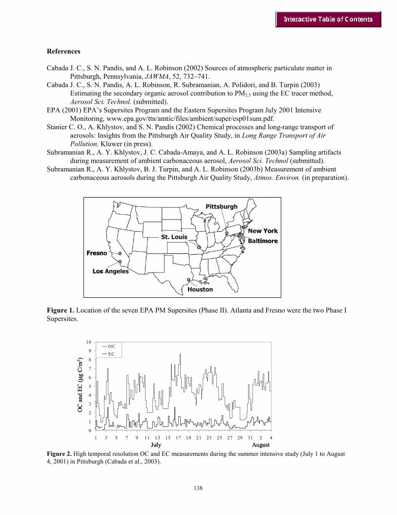
138

References Cabada J. C., S. N. Pandis, and A. L. Robinson (2002) Sources of atmospheric particulate matter in

Pittsburgh, Pennsylvania, JAWMA, 52, 732–741. Cabada J. C., S. N. Pandis, A. L. Robinson, R. Subramanian, A. Polidori, and B. Turpin (2003)

Estimating the secondary organic aerosol contribution to PM2.5 using the EC tracer method, Aerosol Sci. Technol. (submitted).

EPA (2001) EPA’s Supersites Program and the Eastern Supersites Program July 2001 Intensive Monitoring, www.epa.gov/ttn/amtic/files/ambient/super/esp01sum.pdf.

Stanier C. O., A. Khlystov, and S. N. Pandis (2002) Chemical processes and long-range transport of aerosols: Insights from the Pittsburgh Air Quality Study, in Long Range Transport of Air Pollution, Kluwer (in press).

Subramanian R., A. Y. Khlystov, J. C. Cabada-Amaya, and A. L. Robinson (2003a) Sampling artifacts during measurement of ambient carbonaceous aerosol, Aerosol Sci. Technol (submitted).

Subramanian R., A. Y. Khlystov, B. J. Turpin, and A. L. Robinson (2003b) Measurement of ambient carbonaceous aerosols during the Pittsburgh Air Quality Study, Atmos. Environ. (in preparation).

Figure 1. Location of the seven EPA PM Supersites (Phase II). Atlanta and Fresno were the two Phase I Supersites.

Figure 2. High temporal resolution OC and EC measurements during the summer intensive study (July 1 to August 4, 2001) in Pittsburgh (Cabada et al., 2003).

Los Angeles

Fresno

Houston

New York

Baltimore

Pittsburgh

St. Louis

Los Angeles

Fresno

Houston

New York

Baltimore

Pittsburgh

St. Louis

OC

and

EC

(µg

C/m

3 )

AugustJuly

0

1

2

3

4

5

6

7

8

9

10

1 3 5 7 9 11 13 15 17 19 21 23 25 27 29 31 2 4

OCEC

OC

and

EC

(µg

C/m

3 )

AugustJuly

0

1

2

3

4

5

6

7

8

9

10

1 3 5 7 9 11 13 15 17 19 21 23 25 27 29 31 2 4

OCEC

139

Figure 3. Average OC and BC concentrations during the July 2001 intensive in Pittsburgh (Subramanian et al., 2003a) based on five different approaches. All samples were analyzed using the same analytical method.

Figure 4. Estimated average SOA fraction of the measured organic aerosol for Pittsburgh during July 2001 using four different data sets from different samplers. Despite the difference in absolute concentrations, all approaches suggest that roughly 40% of the organic aerosol was secondary and the rest was primary.

0

1

2

3

4

5

Und

enud

edSa

mpl

er(f

ront

quar

tz)

Und

enud

edSa

mpl

er(f

ront

quar

tz-

teflo

nqu

artz

)

Und

enud

edSa

mpl

er(f

ront

quar

tz-

back

upqu

artz

)

Den

uded

In-s

ituA

naly

zer

Den

uded

Sam

pler

OC

and

EC

(µg

C/m

3 )OCBC

UndenudedSampler

(QF)

UndenudedSampler(QF – QB,F)

UndenudedSampler(QF – QB,T)

DenudedIn-Situ

Analyzer

DenudedSampler

(QFden + CIFB,Fden)

0

1

2

3

4

5

Und

enud

edSa

mpl

er(f

ront

quar

tz)

Und

enud

edSa

mpl

er(f

ront

quar

tz-

teflo

nqu

artz

)

Und

enud

edSa

mpl

er(f

ront

quar

tz-

back

upqu

artz

)

Den

uded

In-s

ituA

naly

zer

Den

uded

Sam

pler

OC

and

EC

(µg

C/m

3 )OCBC

UndenudedSampler

(QF)

UndenudedSampler(QF – QB,F)

UndenudedSampler(QF – QB,T)

DenudedIn-Situ

Analyzer

DenudedSampler

(QFden + CIFB,Fden)

0% 20% 40% 60% 80% 100%

Undenuded frontquartz (4-6 hrs)

Undenuded, Q-TQcorrection (4-6 hrs)

Undenuded, Q-Qcorrection (4-6 hrs)

Denuded In-situAnalyzer(2-6 hrs)

140

Figure 5. Sampling sites used in the Pittsburgh Supersite study. Four sites were inside the city of Pittsburgh, while the Florence site was upwind and the Greensburg site was downwind (most of the time). For parts of the study, additional sites existed in Holbrook and Athens.

Figure 6. Daily average sulfate concentrations for July 2001 in the central Pittsburgh site, two more sites inside Pittsburgh, and the two sites outside the city.

Greensburg

Holbrook

Athens

Florence

Greensburg

Holbrook

Athens

FlorenceFlorence

PM 2.5 sulfate

0.0

10.0

20.0

30.0

6/30/0

17/2

/017/4

/017/6

/017/8

/01

7/10/0

1

7/12/0

1

7/14/0

1

7/16/0

1

7/18/0

1

7/20/0

1

7/22/0

1

7/24/0

1

7/26/0

1

7/28/0

1

7/30/0

1

Date

PM2.

5 su

lfate

, ug/

m^3

Florence

Greensburg

Hazelw ood (PIT)

Law renceville (PIT)

Main site (PIT)

141

0.0

0.5

1.0

1.5

6/30/2

001

7/2/20

01

7/4/20

01

7/6/20

01

7/8/20

01

7/10/2

001

7/12/2

001

7/14/2

001

7/16/2

001

7/18/2

001

7/20/2

001

7/22/2

001

7/24/2

001

7/26/2

001

7/28/2

001

7/30/2

001

Date

PM2.

5 EC

, ug/

m^3

FlorenceHazelwood (PIT)Lawrenceville (PIT)Main site (PIT)

Figure 7. Daily average EC concentrations for July 2001 in two sites inside Pittsburgh, and the two sites outside the city. The upwind site (Florence) has the lowest concentrations.

Figure 8. Estimated EC (elemental carbon) emission inventory for the Pittsburgh Metropolitan Area in 1995 (Cabada et al., 1992).

0

40

80

120

160

200

Jan Feb Mar Apr May Jun Jul Aug Sep Oct Nov Dec

Tons

EC

Steel works (coke burning)Heavy Duty TrucksRiver VesselsLight Duty TrucksRailroadStructural firesAircraftResidential WoodburningCatalytic AutosResidential Natural GasTire AttritionOthers

143

Contribution of Local Versus Regional Sources to Exposure

Constantinos Sioutas† University of Southern California,

Department of Civil and Environmental Engineering Introduction

Epidemiological studies have demonstrated a strong link between particulate matter concentrations and health effects (Dockery et al., 1996). However, it is not clear whether it is number, mass or surface area concentrations, or chemical composition that poses the greatest health risk. In an urban environment, there are generally two main contributors to the PM concentrations: primary or direct emissions from particle sources and secondary PM formed by photochemical or physical processes in the atmosphere. The air at a downwind receptor location will contain particles emitted from local sources, as well as particles emitted or formed far upwind that have aged during transport.

The literature on systematic monitoring of the physical and chemical characteristics of ultrafine particles (typically defined as those having diameters below 0.1 µm) in either urban or rural settings has not been as abundant as that for PM2.5 or PM10, mainly because current regulation does not single out the concentration of these particles. Nevertheless, there has been rapidly increasing epidemiological and toxicological evidence linking respiratory health effects and exposures to ultrafine particles (Peters et al., 1997; Pekannen et al., 1997; Li et al., 2002, 2003).

Most of the studies examining the size distributions of PM were conducted in urban areas in which the vast majority of ultrafine PM originates from primary sources (Harrison et al., 2000; Morawska et al., 1998; Woo et al., 2001); thus their diurnal concentration profiles match those of local vehicular sources. The majority of these studies were also intense in nature, ranging for periods of a few weeks to a few months. Depending on the lower detectable particle size of the condensation counter used to detect ultrafine particles, these investigations indicated that the size distribution of a “typical” ultrafine aerosol has a number mean or mode diameter in the range of 20 to 40 nm, and over 90% to 99% of particle counts are associated with particles below 100 nm.

The work presented in this paper intends to add to the body of information on continuous spatial and temporal variations in aerosol parameters such as number, mass, size distribution, and chemical composition in different locations and seasons in one of the most unique air basins of the U.S., the Los Angeles Air Basin (LAB). The research described here is part of the activities of the Southern California Supersite, a large monitoring program funded by the U.S. Environmental Protection Agency (EPA). One of the main objectives of this program is to conduct research that contributes to a better understanding of the measurement, sources, size distribution, chemical composition, physical state, spatial and temporal variability, and health effects of suspended particulate matter (PM). In order to study the geographical and seasonal variation of PM, the primary sampling site was moved to a new location within the LAB every 6 to 12 months. The data analyzed in the current study were collected over the past two years by the sampling activities of the Southern California Particle Center and Supersite (SCPCS). A better understanding of the sources and formation mechanisms of PM with respect to spatial, diurnal, and seasonal variability will aid in the design of future control strategies for PM as well as refine the parameters used in epidemiological studies that attempt to link particulate levels and observed health effects.

† Contributors: USC: Seongheon Kim, Si Shen, Chandan Misra, Philip Fine; UCLA: William Hinds, Yifang Zhu, Andre Nel, Art Cho, John Froines. Funded by: Southern California Particle Center and Supersite (US EPA).

144

Methods The PM data presented in this paper were generated at three types of locations within the LAB.

The sampling locations considered in this work were chosen to represent 3 distinct air pollution regimes: sites in the “zone of influence of freeways,” sites reflective of typical urban areas, and receptor locations of the LAB. These sites are (Figure 1):

• Sites up and downwind of a mostly gasoline-vehicle freeway (I-405) • Sites up and downwind of a freeway with heavy diesel vehicle traffic (I-710) • Source Sites: USC and Downey, located 2 miles south and east of downtown LA, respectively • Several inland “receptor” locations in the LAB (Riverside, Rubidoux, Claremont)

Sampling was conducted during the cooler and warmer seasons in Los Angeles in order to determine the effects of meteorology on PM characteristics. Receptor sites, located towards the east of the LAB, can be considered downwind receptor sites, and are associated with some of the highest PM2.5 concentrations in the US. The sources and formation mechanisms of PM in these sites are also of particular interest. Unlike a typical urban environment, these sites are influenced by local primary sources, the advection of primary, but aged, particulate emissions from areas situated upwind, and the formation of secondary aerosols in the atmosphere. The data collected by several near-continuous instruments are used to infer information on sources and formation mechanisms at each location as well as their prevalence over different times of day and different seasons. Results and Discussion

Size-segregated PM10 mass and chemical composition data from MOUDI and Partisol measurements are presented. Included are results from Downey, Riverside, and Rubidoux. Figure 2 presents MOUDI-collected mass concentrations, by chemical group (Singh et al., 2002). The mass median diameter (MMD) of PM2.5 in Downey (a source area) is smaller than that of Riverside, consistent with the notion of the aerosol in Downey being reliably “fresh” as opposed to “aged”. Similarly, results of the PAH size distributions measured at the two sites, using the regular and the denuded MOUDI configurations, shown in Figure 3, indicate a few striking differences between the size distributions obtained with the regular MOUDI at Downey (source site) and Rubidoux (downwind receptor site) (Eiguren-Fernandez et al., 2003). At the source site, with only one exception—fluoranthene (FLU), the measured PAHs are mostly associated with the ultrafine mode particles. Again, these results are consistent with the fact that the Central Los Angeles area is strongly impacted by fresh vehicular emissions. By contrast, in Rubidoux, except for naphtalene (NAP) and anthracene (ANT), the PAH peaks (Figure 3b) are associated with accumulation mode particles (0.18<dp<2.5 µm). Vehicular emissions in the Rubidoux area are not negligible, but are much smaller compared to those generated by light and heavy-duty vehicles near Central Los Angeles. Except for FLU, the total PAH concentrations measured in the receptor site (Rubidoux) were, on average, about 6 times smaller that at Downey. Previous studies conducted nearby in Riverside (~6 km southeast of Rubidoux) have shown that the fine PM fraction consists mainly of particles generated by atmospheric reactions as well as those that reach this area and were originally emitted in much higher concentrations in the Central Los Angeles area (Pandis et al., 1992; Kim et al., 2002). By the time they reach the Riverside area, after a period on the order of 15-25 hrs, the particles in the air parcel agglomerate to form more stable accumulation mode particles.

PM data collected in the vicinity of freeway sites were also of particular note with respect to human exposure to air pollutants originating from traffic sources. Particle number concentration and size distributions in the size range from 6 to 220 nm were measured by a condensation particle counter (CPC) and a scanning mobility particle sizer (SMPS), respectively, in the vicinity of freeways. Measurements were taken at 30, 60, 90, 150, and 300 m downwind, and 300 m upwind from Interstate 405 at the Los Angeles National Cemetery (Zhu et al., 2002b). The range of average concentration of CO, black carbon, total particle number, and mass concentration at 30 m was 1.7 to 2.2 ppm, 3.4 to 10.0 µg/m3, 1.3 × 105 to 2.0 × 105 /cm3, and 30.2 to 64.6 µg/m3, respectively. For the conditions of these measurements, relative concentration of CO, black carbon, and particle number track each other well as one moves away from

145

the freeway. Particle number concentration (6-220 nm) decreased exponentially with downwind distance from the freeway. Data show that both atmospheric dispersion and coagulation contribute to the rapid decrease in particle number concentration and change in particle size distribution with increasing distance from the freeway. Average traffic flow during the sampling periods was 13,900 vehicles/hr; 93% of vehicles were gasoline-powered cars or light trucks. Measured number concentration tracked traffic flow well. Three distinct ultrafine modes were observed 30 m downwind from the freeway, with geometric mean diameters of 12.6 nm, 27.3 nm, and 65.3 nm. The smallest mode, with a peak concentration of 1.6×105 /cm3, disappeared at distances greater than 90 m from the freeway. Ultrafine particle number concentration measured at 300 m downwind from the freeway was indistinguishable from upwind background concentration. Similar data were also obtained at sites in the vicinity of the I-710 freeway, impacted primarily by heavy-duty diesel traffic, with the most notable difference between the 2 sites being the elemental carbon (EC) levels, which were substantially more elevated in the I-710 freeway (Figures 4-5).

The effect of season on freeway PM characteristics was also investigated. The decay rates of CO and BC are slightly greater in summer than in winter for both freeways suggesting a weaker atmospheric dilution effect in winter (Figure 6) (Zhu et al., 2002a). Particle number concentration in the size range of 6-12 nm is significantly higher in winter than in summer. The associated concentration in that size range decreased at a slower rate in winter than in summer. The surface area concentrations in the size range of 6-220 nm are consistently higher in summer for all sampling locations. These results suggest that wintertime conditions favor greater particle formation, possibly due to increased condensation of organic vapors, coupled with decreased atmospheric mixing depth. The lower degree of atmospheric mixing in the winter may also result in a lower degree of coagulation of nanoparticles. These data may be useful for epidemiological studies to estimate exposure to ultrafine particles in the vicinity of major highways and to evaluate their adverse health effects.

Investigations were also conducted in source and receptor areas of Southern California (Downey and Riverside), in order to examine the effect of different sources and formation mechanisms on the size distribution and temporal trends of ultrafine particles. Near-continuous data were collected for a period of five months at each location. The data clearly identified Downey as a source site, primarily affected by vehicular emissions from nearby freeways, and Riverside as a receptor site, where photochemical secondary reactions form a substantial fraction of particles, along with local vehicular emissions (Kim et al., 2002). In Downey, the diurnal trends of total particle number concentration and elemental carbon appear to be almost identical throughout the day and irrespective of season, thereby corroborating the role of primary emissions in the formation of these particles (Figure 7). This agreement between elemental carbon and particle number was not observed in Riverside during the warmer months of the year, while very similar trends to Downey were observed during the winter months in that area. Similarly, the size distribution of ultrafine particles in Downey is generally unimodal with a mode diameter of 30 to 40 nm and without significant monthly variations. The number-based particle size distributions obtained in Riverside were bimodal, with a significant increase in accumulation mode as the season progresses from winter to summer. During the warmer months, there was also an increase in sub-100-nm particles in the afternoon hours, between 2 PM and 4 PM, that also increased with the temperature. The differences observed in the ultrafine particle distribution and temporal trends clearly demonstrated that mechanisms other than direct emissions play an important role in the formation of ultrafine particles in receptors sites of the LAB (Figure 8.)

The substantial spatial variability of ultrafine PM is of particular note in terms of human exposure and health effects, considering that studies undertaken by the SCPCS also show that these particles appear to be more toxic on a per-mass basis compared to other PM modes. The premise for this series of studies, which occurred concurrently to the collection of the physical and chemical data discussed above, was the increasing awareness that various PM components induce pulmonary inflammation through the generation of oxidative stress. Coarse, fine, and ultrafine particles (UFPs) were collected by ambient particle concentrators in the LAB, and used to assess their chemical composition in

146

parallel with assays to show their redox cycling capacity and ability to generate oxidative stress in macrophages and epithelial cells (Li et al., 2002a). UFPs were most potent towards inducing cellular heme oxygenase-1 (HO-1) expression and depleting intracellular glutathione as markers for oxidative stress. HO-1 expression is directly correlated to the high organic carbon and polycyclic aromatic hydrocarbon (PAH) content of UFPs (Figure 9). The dithiothreitol (DTT) assay, a quantitative measure of reactive oxygen species (ROS) formation was correlated with PAH content and HO-1 expression. UFPs also had the highest ROS activity in the DTT assay. Because the small size of UFPs allows better tissue penetration, we used electron microscopy to study subcellular localization. UFPs and, to a lesser extent, fine particles localize in mitochondria, where they induce major structural damage. This may contribute to oxidative stress. Our studies demonstrate that the increased biological potency of UFPs is related to the content of redox cycling organic chemicals and the ability to damage mitochondria. References Dockery, D. W., Cunningham, J., Damokosh, A.I., Neas, L.M., Spengler, J.D., Koutrakis, P., Ware, J.H., Raizenne,

M., Speizer, F.E. “Health Effects of Acid Aerosols on North American Children: Respiratory Symptoms”. Environmental Health Perspectives, 104: 500–505, 1996

Eiguren-Fernandez A., Miguel A.H, Jaques, P.A. and Sioutas, C. “Evaluation of a Denuder-MOUDI-PUF Sampling System to Measure the Size Distribution of Semivolatile Polycyclic Aromatic Hydrocarbons in the Atmosphere”. Aerosol Science and Technology, 37: 201–209, 2003

Fine, P.M., Si, S., Geller, M.G., and Sioutas, C. “Diurnal and Seasonal Characteristics and Size of Ultrafine PM in Receptor Areas of the Los Angeles Basin”. Aerosol Science and Technology, in press, January 2003

Harrison, R. M., Shi, J.P., Xi, S., Khan, A., Mark, D., Kinnersley, R., and Yin, J. “Measurement of Number, Mass and Size Distribution of Particles in the Atmosphere”. The Royal Society, (358): 2567–2580, 2000.

Kim, S., Shen, S., Sioutas, C., Zhu, Y., and Hinds, W.C. “Size Distribution and Diurnal and Seasonal Trends of Ultrafine Particles in Source and Receptor Sites of the Los Angeles Basin”. Journal of Air and Waste Management Association, 52:297–307, 2002

Li, N., Kim, S., Wang, M., Froines, J.R., Sioutas, C. and Nel, A. “Use of a Stratified Oxidative Stress Model to Study the Biological Effects of Ambient Concentrated and Diesel Exhaust Particulate Matter”. Inhalation Toxicology, 14(5): 459–486, 2002a

Li, N., Sioutas, C , Froines, J.R., Cho, A., Misra, C and Nel, A., “Ultrafine Particulate Pollutants Induce Oxidative Stress and Mitochondrial Damage” Environmental Health Perspectives, in press, 2003

Morawska, L., Thomas, S., Bofinger, N., Wainwright, D., and Neale, D. “Comprehensive Characterization of Aerosols in a Subtropical Urban Atmosphere: Particle Size Distribution and Correlation with Gaseous Pollutants”. Atmospheric Environment, 32 (14-15): 2467–2478, 1998

Pandis, S. N., Harley, R.A., Cass, G.R., and Seinfeld, J.H. “Secondary Organic Aerosol Formation and Transport”. Atmospheric Environment, 26A: 2269–2282, 1992

Pekkanen, J., Timonen, K.L., Ruuskanen, J., Reponen, A., and Mirme, A. “Effects of Ultrafine and Fine Particles in Urban Air on Peak Flow Expiratory Flow Among Children with Asthmatic Symptoms” Environmental Respiratory, 74: 24–33, 1997

Peters, A., Wichmann, H.E., Tuch, T., Heinrich, J., Heyder, J. “Respiratory Effects are Associated with the Number of Ultrafine Particles”. American Journal of Respiratory Critical Care Medicine, 155: 1376–1383, 1997

Singh, M., Jaques, P.A., Sioutas, C. “Size distribution and diurnal characteristics of particle-bound metals in source and receptor sites of the Los Angeles Basin”. Atmospheric Environment, 36(10):1675–1689, 2002

Woo, K.S., Chen, D.R., Pui, D.Y.H., and McMurry, P.H. “Measurement of Atlanta Aerosol Size Distributions: Observation of Ultrafine Particles Events”. Aerosol Science and Technology, 34: 75–87, 2001

Zhu, Y., Hinds, W.C., Kim, S., Shen, S. and Sioutas, C. “Study of Ultrafine Particles near a Major Highway with Heavy-Duty Diesel Traffic”. Atmospheric Environment. 36, 4323–4335, 2002a

Zhu, Y., Hinds, W.C., Kim, S and Sioutas, C. “Concentration and Size Distribution of Ultrafine Particles near a Major Highway”. Journal of Air and Waste Management Association, 52:1032–1042, 2002b

147

Figure 1. Source and receptor areas in the Los Angeles basin. Copyright from Evaluation of a denuder-MOUDI-PUF sampling system to measure the size distribution of semi-volatile polycyclic aromatic hydrocarbons in the atmosphere by Diguren-Fernandez et al. Reproduced by permission of Taylor & Francis, Inc, http://www.routledge-ny.com.

Figure 2. Average 24-hr PM10 mass and chemical composition in Riverside (top) and Downey (bottom)

2 4 - h A v e r a g e P M 1 0 M a s s a n d C h e m ic a l C o m p o s it io n in D o w n e y

0

2

4

6

8

1 0

1 2

1 4

2 . 5 - 1 01 - 2 . 50 . 3 5 - 1 . 00 . 1 - 0 . 3 5< 0 . 1

P a r t i c le S iz e R a n g e , m ic r o n s

Con

cent

ratio

n (µ

g/m

3)

M e t a l sO CE C( N H 4 ) 2 O S 4N H 4 N O 3

S i n g h e t a l A t m o s p h e r i c E n v i r o n m e n t , 3 6 ( 1 0 ) : 1 6 7 5 - 1 6 8 , 2 0 0 2

M M D ~ 0 . 3 5 u m

24-h Average PM10 Mass and Chemical Composition in Riverside (top) and Downey (bottom)

0

2

4

6

8

10

12

14

2.5 - 101 - 2.50.35 - 1.00.1 - 0.35< 0.1

Size range, microns

conc

entr

atio

n ( ?g

/m3)

metals

OC

EC

(NH4)2SO4NH4NO3

24-h Average PM10 Mass and Chemical Composition in Riverside (top) and Downey (bottom)

0

2

4

6

8

10

12

14

2.5 - 101 - 2.50.35 - 1.00.1 - 0.35< 0.1

Size range, microns

conc

entr

atio

n ( ?g

/m3)

metalsOC

EC

(NH4)2SO4NH4NO3

MMD ~ 0.7 um

AtascaderoLompoc

Riverside

USC

MLUpland

SD

Boyles Height

AtascaderoLompoc

Riverside

USCUSC

MLUpland

SD

Boyles Height

148

Figure 3. Effect of transport on PAH size distribution

Figure 4. Relative Particle Number, Mass, Black Carbon, CO Concentration, vs. Downwind Distance from Freeway 405. JOURNAL OF THE AIR & WASTE MANAGEMENT ASSOCIATION by ZHU Y, HINDS WC, KIM S, SIOUTAS C. Copyright 2002 by AIR & WASTE MGMT ASSN. Reproduced with permission of AIR & WASTE MGMT ASSN in the format Other Book via Copyright Clearance Center.

Riverside Regular MOUDI - Aug.-Oct. 2001

0.0

0.2

0.4

0.6

0.8

1.0

FLT PYR BAA CRY BBF BKF BAP DBA BGP IND

D o w n e y R e g u la r M O U D I - A u g .- O c t. 2 0 0 0

0 . 0

0 . 2

0 . 4

0 . 6

0 . 8

1 . 0

F L T P Y R B A A C R Y B B F B K F B A P D B A B G P IN D

Figure 3. Effect of transport on PAH size distribution

Frac

tion

by m

ass

Frac

tion

by m

ass

Figure 5. Ultrafine size distributions at different sampling locations near the 710 freeway in (a) summer and (b) winter. Reprinted from Zhu et al (2000) with permission from Elsevier.

Figure 6. Elemental Carbon (EC) concentrations as function of distance for the 405 (gasoline) and 710(diesel) traffic freeways. Reprinted from Zhu et al (2000) with permission from Elsevier.

Figure 7. Diurnal Particle Number(PN) and Elemental Carbon (EC) Concentrations in Downey, CA from October, 2000 to January 2001. JOURNAL OF THE AIR & WASTE MANAGEMENT ASSOCIATION by KIM S, SHEN S, SIOUTAS C, ZHU Y, HINDS WC, Copyright 2002 by AIR & WASTE MGMT ASSN. Reproduced with permission of AIR & WASTE MGMT ASSN in the format Other Book via Copyright Clearance Center.

Figure 8. Ultrafine PM modes in Riverside on May 16, 2001. JOURNAL OF THE AIR & WASTE MANAGEMENT ASSOCIATION by KIM S, SHEN S, SIOUTAS C, ZHU Y, HINDS WC, Copyright 2002 by AIR & WASTE MGMT ASSN. Reproduced with permission of AIR & WASTE MGMT ASSN in the format Other Book via Copyright Clearance Center.

0

2000

4000

6000

8000

0 6 12 18 24

Hour of the Day

Par

ticle

Num

ber C

once

ntra

tion

(par

ticle

s/cm

3)

0

2

4

6

8

EC

(µg/

m3 )

PN

EC

Direct Vehicular Emissions are not the only source of Ultrafine PM (UFP)

Data in Riverside (May 16, 2001; Kim et al., JAWMA52:174-185, 2002)

Larger UFP Mode:Advection from Upwind Urban LA

Smaller UFP Mode:Photochemistry

0

5 0 0 0

1 0 0 0 0

1 5 0 0 0

1 0 1 0 0 1 0 0 0

dN/d

logD

p

(par

ticle

s/cm

3 )

( a ) 1 2 P M

0

5 0 0 0

1 0 0 0 0

1 5 0 0 0

1 0 1 0 0 1 0 0 0

dN/d

logD

p

(par

ticle

s/cm

3 )

( b ) 2 P M

0

5 0 0 0

1 0 0 0 0

1 5 0 0 0

1 0 1 0 0 1 0 0 0

dN/d

logD

p

(pas

rticl

es/c

m3 )

( c ) 4 P M

0

5 0 0 0

1 0 0 0 0

1 5 0 0 0

1 0 1 0 0 1 0 0 0

P a r t ic le D ia m e t e r ( n m )

dN/d

logD

p

(par

ticle

s/cm

3 )

( d ) 6 P M

f ix e d a t 1 6 4 n md g = 3 9 n m3 2 % o f t o ta l n u m b e r

d g = 5 5 n m6 5 % o f t o ta l n u m b e r



F ig u r e 1 2 . S im u la te d s u b - m o d e s o f p a r t ic le s in t h e a f t e r n o o n : R iv e r s id e , 5 / 1 6 / 2 0 0 1 .

151

0

1 0

2 0

3 0

4 0

5 0

0

1 0

2 0

3 0

4 0

5 0

∅ 2 5 5 0 1 0 0 2 5 5 0 1 2 2 5 5 0 1 0 0 2 5 5 0 1 0 0 8

C o a r s e F in e U F P C o a r s e F in e U F P

Rel

ativ

e Sc

anni

ng D

ensi

ty

C L - J a n 0 2 U S C - J a n 0 2

C o a r s e

F in e

U F P

C o a r s e

F in e

U F P

D o s e : µ g /m l

H O -1

0

1 0

2 0

3 0

4 0

5 0

0

1 0

2 0

3 0

4 0

5 0

∅ 2 5 5 0 1 0 0 2 5 5 0 1 2 2 5 5 0 1 0 0 2 5 5 0 1 0 0 8

C o a r s e F in e U F P C o a r s e F in e U F P

Rel

ativ

e Sc

anni

ng D

ensi

ty

C L - J a n 0 2 U S C - J a n 0 2

C o a r s e

F in e

U F P

C o a r s e

F in e

U F P

D o s e : µ g /m l

H O -1

C o a r s e

F in e

U F P

C o a r s e

F in e

U F P

D o s e : µ g /m l

H O -1

U F P a t m u c h lo w e r c o n c e n t r a t io n s

Figure 9. UFP Induce Much Higher Oxidative Stress

Data Analytic Procedures for Monitoring Specific Pollutants in

Epidemiological Studies

Richard L. Smith∗

December 31, 2002

Abstract

This note describes some statistical procedures relevant to studying the effect of a specificpollutant, such as emissions from diesel fuel, in epidemiological studies. After some initialremarks about the formulation of the problem in statistical terms, we consider two methodologiesin detail. The first concerns exposure modeling via spatio-temporal interpolation of a pollutantbased on a limited network of monitors. The second is about the assessment of health effectswhen data on multiple constituents of air pollution data are available; an example is given basedon data from Phoenix, where data on PM2.5 broken into individual elements were available.However the discussion also highlights the inadequacy of many existing data bases for this kindof study.

1 Introduction: What is the Question?

Time series studies of air pollution and health, such as the NMMAPS study (Samet et al. 2000a,2000b), are designed to answer questions about the short-term impact (e.g. excess numbers ofdeaths per year) of an atmospheric pollutant, such as PM10 or PM2.5, on some measure of humanhealth. Similarly, prospective studies (Krewski et al. (2000)), which attempt to measure long-termas well as short-term effects, are ultimately designed to assess the total impact on the humanpopulation of some aspect of air pollution health effects. It seems to me that the ultimate objectiveof research in diesel fuel emissions, or any other specific component of air pollution, is to answersimilarly broad-brush questions of total impact on human health, but restricted to that componentof the total pollution. I emphasize this point because the effective design of an epidemiologicalstudy depends on a clear articulation of its objectives. By focussing on these objectives and thekind of statistical analysis needed to achieve them, we gain insight into the data that need tobe collected, and the sample sizes required to answer the questions of interest with a satisfactorydegree of precision.

In the case of diesel pollution, a key aspect seems to be that it is not possible to measuredirectly the emissions of diesel fuel: realistic methods of measurement depend on proxies, such asthe concentrations of certain chemical markers in the ambient air, from which we can infer thediesel emissions with some measurement error.

The effect of measurement error in epidemiological studies of air pollution is one of the knowndifficulties of this area of research. It is widely acknowledged that pollution measured by ambient air

∗Department of Statistics, University of North Carolina, Chapel Hill, NC 27599-3260; [email protected]. Pre-sented at the HEI Workshop to Improve Estimates of Diesel and Other Emissions in Epidemiologic Studies, Baltimore,December 4–5 2002. This paper is based in part on research supported by EPA Cooperative Agreement CR-827737-01-0 and by NSF grants DMS-9971980 and DMS-0084375.

153

monitors differs substantially from that measured by personal monitors, and some limited attemptshave been made to account quantitatively for the effect this has on regression relationships (e.g.,Dominici et al. (2000)). If proxy variables are used for diesel emissions, then the question of howto deal with measurement error is central to the analysis. A typical analysis may use the followingvariables:

X: Measured air pollution variables (e.g. criteria pollutants, PM2.5, specific chemical markers)Y : Response, e.g. mortality, hospital admissions due to asthma,Z: True variable of interest, e.g. diesel emissions

We would like to fit a model of the form

f(Y ) = βZ + other fixed effects + random error (1)

where f(Y ) is some function of the response Y , and the other fixed effects include confounders suchas meteorology, terms to represent time trends and seasonal effects, etc. The measurement errorproblem arises because in epidemiological studies, we are not able to measure Z directly but mustuse X as a set of proxy variables.

However, we also have available training data (e.g. from supersites) that can allow us to studyin detail the joint distributions of X and Z. With this information, the probability distributionswe need to specify are

1. p(X|Z), the distribution of X given Z — this may come from detailed chemical analyses

2. p(Z), the prior distribution of Z — this is needed for Bayesian analyses

Using Bayes’ Theorem, the last two distributions may be combined to produce p(Z|X), theconditional distribution of Z given X. This in turn may be combined with (1) to produce aposterior distribution of β.

This approach, being explicitly Bayesian and taking into account the uncertainty of our knowl-edge about Z, is different from the conventional non-Bayesian approach to measurement error inregression. While there is much room for discussion about details, I believe that an approach ofthis broad structure is needed to take account of the different sources of uncertainty.

Two questions are:

1. What should X be? — In other words, what are the best variables to use as proxies for dieselfuel? Possibly that question is already answered by other presentations at this workshop, buta balance may need to be struck between using a good chemical marker and one that is easyand cheap to measure on the extensive scale needed for a good epidemiological study.

2. What kind of information should be use to assess p(Z)? A crude measure might be based ontraffic patterns, but perhaps something more sophisticated is needed.

2 Spatial Statistics

One way of reducing measurement error would be if we had better methods of spatial interpolationbetween monitors. Patrick Kinney, at this workshop, has highlighted some of the difficulties withdiesel particulate matter (DPM) in comparison with the more extensively studied fine particulatematter (PM2.5). The spatial-temporal variability of PM2.5 is dominated by the temporal component— at any fixed point in time, the field tends to be fairly homogeneous spatially, and this makes it

154

relatively easy to interpolate based on a limited set monitors. With DPM, it appears, the situationis reversed — the variability is dominated by the spatial component. Limited studies with personalmonitors have highlighted the difficulty of interpolating DPM.

There is no ready answer to this problem, but in a recent study, Smith et al. (2003) haveproposed a new approach to interpolating PM2.5, and this method may provide some clues as tohow to deal with the harder problem of DPM.

This particular analysis was based on one year’s PM2.5 data from 74 monitors in three southernstates (NC, SC, GA). Weekly averages were computed based on data available at each monitor.Also available were the latitude-longitude coordinates of the monitor, and a “land use” variable(agricultural, commercial, forest, industrial or residential). Preliminary analysis of the data sug-gested showed a strong weekly variability common to all sites, but with upward or downward shiftsdepending on the characteristics of the sites (Fig. 1).

A model was fitted of the form

yst = ωt + ψs + `s + ηst (2)

where yst is the square root of PM2.5 for week t at site s (the square root transformation was foundto improve the fit of the model), ωt is a week effect, ψs represents a fixed spatial component ofthe variability, `s is a land-use effect (one value for each of the five possible land uses) and ηst

is a random component. The “spatial interpolation” aspect of this only applies to ηst, the othercomponents being regarded as fixed. The parameters ωt and `s were treated as fixed effects, similarto an analysis of variance, while ψs was modeled as a smooth function of s through a thin-platespline representation.

As an example of the output of this analysis, a map of overall mean PM2.5 was produced,and compared with the (much rougher) map produced by simply averaging and interpolating theraw values (Fig. 2). Another feature of the spatial analysis, not possible with non-statisticalinterpolation methods, is the possibility of creating a standard error map (Fig. 2(b)). This wouldbe needed to pursue the kind of analysis discussed in Section 1: for example, if Z represents thePM2.5 at a specific location, and X represents a set of PM2.5 measurements from monitors, then theconditional distribution p(Z|X) involves some measure of variability and not just the conditionalmean of Z given X.

It is conjectural whether a similar technique could be applied to the interpolation of DPM.However, some features of the method should be noted. It has been pointed out that for DPM,although the spatial variability is typically much higher than for PM2.5, the pattern of spatial vari-ability seems to be fairly constant in time (for example, because of consistent traffic patterns). Thissuggests that a model of the form (2), in which there is a fixed term ψs to represent the consistentspatial pattern of observations, would do much better than simple geostatistical interpolation ofthe spatial field at each time point. The method is also well adapted to missing data, since typically(even with PM2.5 data) observations are not available from all monitors at all time points.

3 PCA, Empirical Bayes and Related Methods

We now turn to a different aspect of the analysis, using examples based on Kim et al. (1999), Smithet al. (2000), in which PM10 and PM2.5 data were available from the Phoenix site (1995–1997),along with data on the contributions of individual chemical elements to the PM2.5 total. Dailymortality and meteorological data were also available. The challenge in this study was how toincorporate a large number of possible covariates into a regression analysis.

155

(a)

Week�

Mea

n P

M

0 10 20 30 40

0

20

40

60

(b)

Week�

Mea

n P

M0 10 20 30 40

0

20

40

60

N

NNN

N

NNNNNNNNNNNNNNNNNNNNNNN

N

NNNNNNNNNNNNNNNNNNNNNNNNNNNN

NNNNNNNNNNNNNNNNNNNNNNNNNN

NNNNNNNNNNNNNNNNNNNNN

NNNNN


NNNNNNNNNNNNNNNNNNNNNNNNN

N


N


NNNNNNNNNNNNNNNNNNNNNNNNNNN

N


N

NNNNNNNNNNNNNNNNNNNNNNNNNNNNNNNN

NNNNNNNNNNNNNNNNNNNNNNNNNNNNNN

NN


NNNNNNNNNNNNNNNNNNNNNNNNNNNNNNN

N



N


NNNNNNNNNNNNNNNNNNNNNNNNNNNNN

N






N



NNNNN

NNNNNNNNNNNNNNNNNNNNNNNNNNNNNNNNN

NNNNNNNNNNNNNNNNNNNN

NNNN

NNNNNN


N



N


N

NNNNN


NNN


N






NNNNNNNNNNNNNNNNNNNNNNNN

NNN

NNNN

NNNN

NN

N

(c)

Week

Mea

n P

M

0 10 20 30 40

0

20

40

60

S

SSS

SSSSS

SSSSSSSSSSS

S

SSSSSSSS

SS

SSSSSSSSSS

S

S

SSSSSSSSSS

S

SSSSSSSSS

S

SSSSSSSSSS

SSSSSSSSSSSS

SSSSSSSSSSSS

SSSSSSSSSSS

SSSSSSSSSSS

S

SSSSSSSSSSSS

SSSSSSSSSSSS

SSSSSSSSSSSSS

S

SSSSSSSSSSSS

SSSSSSSSSSSSS

SSSSSSSSSSSSSS

SSSSSSSSSSSSSS

SSSSSSSSSSSSS

S

SSSSSSSSSSSSS

SSSSSSSSSSSSSS

SSSSSSSSSSSSSSS

SSSSS

SSSSSSSSSSS

SSSSSSSSSSSSSS

SS

SSSSSSSSSSSSSSSS

SSSSSSSSSSSSSSSS

SSSSSSSSSSSSSSSS

SSSSSSSSSSSSSSS

S

S

SSSSSSSSSSSSSSS

SSSSSSSSSSSSSSS

S

S

SSSSSSSSSSSSSSS

SSSSSSSSSSSSSSSS

SSSSSSSSSSSSSSS

S

S

SSSSSSSSSSSSSSS

SSSSSSSSSSS

SSSSS

SSSSSSSSSSSSSSSS

SSSSSSSSSSSSSSSS

SSSSSSSSSSSSSS

S

SSSSSSSSSSSSSSS

S

SSSSSSSSSSSSSSSS

SSSSSSSSSSSSSSSS

SSSSSSSSSSSSSSSS

S

SSSSSSSSSSSS

SS

SSSSSSSSSSSSSSSS S

SSSSSSSSSSSSSSS

SSSSSSSSSSSSSSS

S

SSSSSSSSSSSSSSS

SSSSSSSSSSSSS

(d)

Week

Mea

n P

M

0 10 20 30 40

0

20

40

60

G

G

G

GGG

GGG

G

GGGGGGGGGGGG

GGGG

GGG

GGGGG

GGGGGGGGGGGGGG

G

G

GGGGGGGGGGGGGGGGG

GGGGGGGGGGGGGGGG

GGGGGGGGG

GGGGGGGGG

G

GGGGGGGGGGGGGGGGGG

G

GGGGGGGGGGGGGGGGGGGG

GGGGGGGGGGGGGGGGGGGGG

G

G

GGGGGGGGGGGGGGGGGG

GG

GGGGGGGGGGGGGGGG

G

G

G


GGGGGGGGGGGGGGGGGGGGGG

G


GG

G

G


G

GGGGGGGGGGGGGGGGGGGGGGG

GG


GGGGGGGGGGGGGGGGGGGGGGG


G

GG


G


G



G


G


G


GG


G

GGGGGGGGGGGGGGGGG

G

G


G

GGGGGGGGGGGGGGGGG

G

G

G

GG

GGGGGGGGGGGGGGGGG

G

GGGGGGGGGGGGGGGGGGG

G

G


G

G

GG

GGGGGGGGGGGGGGGGGGG


G

G



(e)

Week

Mea

n P

M

0 10 20 30 40

0

20

40

60

A

AAA

A�AAA�

A

AA

AAAA

A

A�AAA�A

AAAAA

AAA�A�

AAAA�A�

AAAA

AAAAAAAA

AAAAA

AAAA�A�

AA

AA

A

AAA

AA

A�A�AA

A

AAAA

A�AAA�AA AA

�AAA

A

AAAAA

A�AAA

A

AA

AAA

A

AAAAAA

A

AAAA

A�

AA

A

AA

AAAA

AA

A�AAA

A�

A�

AAAAAA

A

AA

A

A�A�

A

AAAA

A

AAAA

A

A

AA�A�AAA

A

AAAA

AAAA

AA

AAAA

A�

A

AAAAA

A

A�

AA�A�A�

AAA�AA

A�

AAAAAAA

AA

AAA A

AA

A

A�A�

A

AA

A

AA

AAA

AAA

A�A�A

(f)

Week

Mea

n P

M

0 10 20 30 40

0

20

40

60

C

C

CCCCCCCC

C

CCCCCCCCCC

C

C

CCCCCCCCCCCCC

C

CCCCCC

CCCCC

CCCCCCCCCCCC

C

C

CCCCCCCCCCCCCCC

CCCCCCCCCCCC

CCCCCCCCCCC

CCC

C

CCCCCCCCCCC

C

CCCCCCCCCCCCCCC

CCCCCCCCCCCCCCCCC

C

CCCCCCCCCCCCCCC

C

C

C

CCCCCCCCCCCCC

C

C

CCCCCCCCCCCCCCCCCC

CC

CCCCCCCCCCCCCCC

C

CCCCCCCCCCCCCCCCCCC

CCCCCCCCCCCCCCCCC

C

CCCCCCCCCCCCCCCCC

CCCCCCCCCCCCCCCCCC

CCCCCCCCCCCCCCCCC

CCCCCCCCCCCCCCCCCC

CCCCCCCCCCCCCCCCCC

CCCC

CCCCCCCCCCCCC

C

CCCCCCCCCCCCCCCCCC

CC

CCCCCCC

CCCCCCCCC

CCCCCCCCCCCCCCCCCCC

CC

C

CCCCCCCCC

CCCC

CCCCCCCCCCCCCCC

CCCCCCCCCC

CCCCCC

CCCCCCCCCCCCC

C

C

CCCCCCCC

CCCCCCC

CC

CC

CCCCCCCCC

C

C

CC

C

CCCCCCCCCCCC

CCC

CC

CCCCCCCCCC

C

CCCCCCCCCCCC

CCCC

CCC

CCCCCCC

CCCCCC

CCCCCCCCCCCCCCCC

C

CCCCCCCCCCCCCC

CCCCCCCCCCCCCCC

CC

CC

CCCCC

C

CC

CCC

CC

C

CCC

C

CC

CCC

(g)

Week

Mea

n P

M

0 10 20 30 40

0

20

40

60

F

FF F

FF

F

F

F

FF

FF F

F

FF

FF

F

FF

FFF

F

F

F

FF

F

FFF

F

F

F

F

FF

F F

F

F

F

F

F

FF F

F

FF

F

F

F

FF

F

FF

FF

F

F

F

F

F

FF

F

FF

F

FF

FF

F

FF

FF

F F

F

FF F

F

F

F

FF

FF

F

F

F

F F

(h)

WeekM

ean

PM

0 10 20 30 40

0

20

40

60

I

I

II

I

I

IIIII

I

I

III

II

IIIII

II

IIIIII

I

I

IIIIII

II

I

IIIIIIII

IIIIII

I

II

IIIIII

IIII

IIIIIIII

I

IIIIIIIIII

IIIIIIII

I

IIIIII

III

I

IIIIIIIII

IIIIIIIIII

IIIIIIII

I

I

I

IIIIIIII

IIIIIIIIII

IIIIIIIIII

IIIIII

II

II

IIII

III

II

I

IIIIIIIII

I

II

III

II

III

IIII

III

II

II

IIIIII

I

I

IIIIIIII

IIIIIII

II

IIIIIIIII

IIIIIIII

I

IIIII

IIII

IIII

I

II

I

I

IIIIIII

II

IIIIIIIII

IIIIIIIII

I

II

II

IIII

I

II

II

IIIII

IIIIIIIIII

IIIIIIIIII

IIIIIIIII

III

I I II

I

I

(i)

Week

Mea

n P

M

0 10 20 30 40

0

20

40

60

R

RRRR

R

RRRRRRRRRRRRRRRRR

RRRRRRRRRRRRRRRRRRRR

RRRRR

RRRRRRRRRRRRRRRRRR

RRRRRRRRRRRRRRRRRRRRR

RR

RRRRRRRRRRRRRRRRRRRRRRRRRR

RRRRRRRRRRRRRRRRRRRRRRRR

RRRRRRRRRRRRRRRRRRRRRRRRR

R

RRRRRRRRRRRRRRRRRRRRRRRRRRRR

RRRRRRRRRRRRRRRRRRRRRRRRRRRRRR

R


RRRRRRRRRRRRRRRRRRRRRRRRRRRRRRR

R




R

RRRRRRRRRRRRRRRRRRRRRRRRRRRRRRRR

RRRRRRRRRRRRRRRRRRRRRRRRRRRRRRRRR




RRRRRRRRRRRRRRRRRRRRRRRRRRRRRRRRRR


RR


RRR


RRRRRRRRRRRRRRRRRRRRRRRRRRRRRRRRRRR


R

R

R


R

RR

RRRRRRRRRRRRRRRRRRRRRRRRRRRRR

RRR


R

RR



RRR

R


RR

R

RR


R

R


R

RR


R


R

RRR



R



RR

RRRRRRRR

RR

RRRRRRRRR

R

RRRRRRRRRRR

RRRRRR

RRRRRRR

R

RRRRRRR

RRRRRR

R

RRRRRRRRR

RRRR

Figure 1. Comparison of fitted trend and raw data for subpopulations. (a) All data combined,(b) NC, (c) SC, (d) GA, (e) Agricultural sites, (f) Commercial, (g) Forest, (h) Industrial, (i)Residential. A single common weekly trend is shown (same on all plots), with superimposed datapoints from the individual stations in each subpopulation.

10 16 22�

(a) Mean PM2.5 Surface

0.8 1.2 1.6

(b) Standard Error Surface

12 16 20�

(c) Raw PM2.5 Means

Figure 2. Reconstructed surface for overall annual mean PM2.5. (a) Mean surface. (b) Standarderror. (c) Plot of raw data with linear interpolation on a triangulation (S-PLUS “interp” routine).

156

• • • • • ••

•• • • • •

• • ••

•• • •

-0.6

-0.4

-0.2

0.0�

0.2�

0.4�

•

•

• ••

•

•

•

•

• •

•• • •

•

•

• ••

•• • • • • ••

• •• •

•• • •

••

• • ••

AL�

SI P S CL K CA SC TI�

V CR MN FE CO NI CU ZN�

GA GE AS�

SE

• •• • • • • • • •

• • • • •• •

• • • •

-0.6

-0.4

-0.2

0.0�

0.2�

0.4�

•

•• • • • • • • • •

•

••

•

•

•• • • ••

•• • • • • • •

••

•• • •

• • • • • •

BR RB SR Y�

ZR�

MO RH PD AG�

CD SN SB TE�

I CS BA LA W �

AU�

HG PB

Figure 3. Estimates and 95% confidence bands obtained for each of 42 elements. Three estimatesfor each element: (left) ordinary least squares (OLS) estimates when elements are added one ata time; (middle) OLS estimate when elements are added all together; (right) Ridge regressionestimates.

One conclusion that contradicted conventional wisdom on air pollution health effects was thatfor this data set, it appeared that the effect due to coarse particles (difference between PM10 andPM2.5) was stronger than that due to PM2.5, though the PM2.5 effect was significant above athreshold in the region of 20–25 µg/m3 (Smith et al. (2000)).

In further analysis, we considered regressions in which the covariates of a pollution-mortalityrelationship included the measured concentrations (for 300 days of data) of 42 chemical elements.In Fig. 3, the regression coefficients and 95% confidence limits are plotted, computed three differentways: (a) putting in the 42 elements one at a time (the left-hand member of each group of threeestimates), (b) including all 42 elements at once (middle), (c) including all 42 elements but reducingthe variability of the estimates by ridge regression (right). Method (a) produces reasonable-lookingestimates, but the difficulty is that we do not believe that any single element is responsible for

157

the mortality effect: the intention behind the analysis is to identify groups of elements, or specificcombinations of elements, that might act as some kind of marker. The analysis (b) includes allthe elements, but many of the individual estimates have very large standard errors as indicated bythe length of the vertical bars. Ridge regression, method (c), is a method described in many textson regression analysis, that aims to reduce the variability of the individual estimates at the costof introducing a small amount of bias. In this case, the ridge estimates are quite similar to thesingle-variable estimates in (a), and apparently superior to those in (b).

Ridge regression is just one of a number of so-called shrinkage methods that have been designedto improve the performance of regression estimates when there are very many regressors or a highdegree of multicollinearity. Other methods include the lasso method (Tibshirani 1996), variousmethods developed in the context of calibration (Brown 1993), and empirical Bayes methods (Carlinand Louis 1996). As an example of the latter, Kim et al. (1999) adapted the triple-goal estimatesof Shen and Louis (1998) to this regression setting.

For this particular data set, none of the methods was successful in identifying any particularelement or group of elements that was especially strongly associated with pollution health effects,a conclusion that was scarcely surprising given the overall weak association between PM2.5 andmortality in this data set.

For an alternative analysis, Smith et al. (2000) looked at seasonal effects with a view toexamining whether seasonal patterns in the PM-mortality effect could in any way be associated withseasonal pattern in the pollutants. Table 1 shows seasonal coefficient estimates for the mortalityeffect of coarse PM (the corresponding results for fine PM showed no evidence of any seasonaleffect). The effects are strongest in the spring and summer.

Season Mean coarse Regression Standard t statistic p valuePM (µg/m3) Coefficient Error

Winter 33.6 0.0036 0.0023 1.5 0.13Spring 28.9 0.0139 0.0026 5.3 0.0001

Summer 31.6 0.0063 0.0026 2.4 0.018Fall 39.3 0.0023 0.0022 1.0 0.3

Table 1. Effect of coarse PM on mortality, measured by season.

A subset of the single-element data (Al, Si , S, Ci, K, Ca, Ti, Mn, Fe, Cu , Zn, Pb) was furtherclassified using a principal components analysis which showed that the crustal elements (Al, Si,K, Ca, Ti, Mn, Fe) explained 55% of the variation of coarse PM, the anthropogenic elements (Fe,Cu, Zn, Pb) explained 30%, and the elements of marine origin (Cl in NaCl; Na was not measured)explained 5%. Table 2 shows a breakdown by season of the means of three principal componentscorresponding to each of these groups.

Season Crustal Anthropogenic MarineWinter –.144 .503 –.589Spring –.278 –.323 .073

Summer .004 –.483 .41Fall .245 .222 .03

Table 2. Breakdown by season of mean level of each of the three principal groups of elements(standardized to overall mean 0 for each component)

It appears that the seasons in which the anthropogenic effect is low are also the ones withhighest effect due to PM. This is, of course, contrary to the common understanding that the effect

158

of naturally occuring particulate matter in the atmosphere is much less important than the effectof industrial and other anthropogenic sources. There may be some natural explanation of thisphenomenon in the case of Phoenix, or the whole result may just be an artifact of the relativelysmall scale of the study, but either way, it suggests questions for further study.

4 Summary and Conclusions

Any meaningful attempt to integrate measures of diesel emissions into large-scale epidemiologicalstudies will have to deal up front with the issue of bias induced by measurement error. Section 1 ofthis discussion has outlined a possible conceptual approach and some of the main issues that needto be addressed in order to apply it.

One aspect of measurement error bias comes from the fact that any measure of air pollutionis only available at ambient monitoring sites and these are not typically in good agreement withmeasurements derived from personal exposure monitors. This is an issue with studies based onPM2.5, but is expected to be a much more serious issue with measures of diesel fuel emissionsbecause of the much greater spatial variability of the latter compared with PM2.5. In Section 2,I have outlined some current thinking about the spatial interpolation of PM2.5, which improvesubstantially on simple geostatistical methods, and may be applicable to other pollutants as well.

Section 3 of this discussion has highlighted some of the issues involved in regression analysisof pollution-mortality relationships when there are a large number of pollution-related covariates,represented here by the individual elements in chemical analyses of PM2.5. Ordinary least-squaresregression estimates do not perform where when there are many covariates and/or a high degree ofmulticollinearity. Alternative methods such a ridge regression or empirical Bayes analysis are avail-able, and may be expected to improve the simultaneous estimation of many regression coefficients.These methods will not help with very limited data sets. The biggest obstacle to this whole fieldof research, as I see it, is designing and collecting data for epidemiological studies on a sufficientlylarge spatial-temporal scale to make meaningful health effects estimates.

5 References

Brown, P.J. (1993), Measurement, Regression and Calibration. Oxford University Press.Carlin, B.P. and Louis, T.A. (1996), Bayes and Empirical Bayes Methods for Data Analysis.

Chapman and Hall, London.Dominici, F., Zeger, S.L. and Samet, J.M. (2000), A measurement error model for time series

studies of air pollution and mortality. Biostatistics 1, 157–175.Kim, Y., Spitzner, D., Zhang, Z., Smith, R.L. and Fuentes, M. (1999), Accounting for multiple

pollutants in pollution-mortality studies. Proceedings of the ASA Biometrics Section, 1–10.Krewski, D., Burnett, R.T., Goldberg, M.S., Hoover, K., Siemiatycki, J., Jerrett, M., Abra-

hamowicz, M. and White, W.H. (2000), Reanalysis of the Harvard Six Cities Study and the Amer-ican Cancer Society Study of Particulate Air Pollution and Mortality. A Special Report of theInstitute’s Particulate Epidmiology Reanalysis Project. Health Effects Institute, Cambridge, MA.

Samet, J.M., Dominici, F., Zeger, S.L., Schwartz, J. and Dockery, D.W. (2000a), Nationalmorbidity, mortality and air pollution study. Part I: methods and methodologic issues. ResearchReport 94, Health Effects Institute, Cambridge, MA.

Samet, J.M., Zeger, S.L., Dominici, F., Curriero, F., Coursac, I, Dockery, D.W., Schwartz,J. and Zanobetti, A. (2000b), National morbidity, mortality and air pollution study. Part II:

159

morbidity, mortality and air pollution in the United States. Research Report 94, Health EffectsInstitute, Cambridge, MA.

Shen, W. and Louis, T.A. (1998), Triple-goal estimates in two-stage hierarchical models. J.R.Statist. Soc. B 60, 455–471.

Smith, R.L., Kim, Y., Fuentes, M. and Spitzner, D. (2000), Threshold dependence of mortalityeffects for fine and coarse particles in Phoenix, Arizona. Journal of the Air and Waste ManagementAssociation 50, 1367–1379.

Smith, R.L., Kolenikov, S. and Cox, L.H. (2003), Spatio-temporal modeling of PM2.5 data withmissing values. Tentatively accepted for Journal of Geophysical Research–Atmosphere.

Tibshirani, R. (1996), Regression shrinkage and selection via the lasso. J.R. Statist. Soc. B58, 267–288.

160

Appendix: HEI Workshop to Improve Estimates of Diesel and Other Emissions for Epidemiologic Studies

Marriott Baltimore WaterfrontBaltimore, Maryland December 4-5, 2002

Agenda

Wednesday December 4 (Dover ABC)

9:00 AM Welcome Dan Greenbaum, Health Effects Institute

9:10 AM Context setting Ted Russell, Georgia Institute of Technology

9:25 AM Necessary attributes for a signature for health effects studies Jonathan Samet, Johns Hopkins University


9:45 AM Issues in retrospective epidemiology studies and lessons learned in assessing exposure Eric Garshick, Brigham &Women's Hospital

10:15 AM Issues in exposure assessment in epidemiologic studies of acute effects Patrick Kinney, Columbia University Mailman School of Public Health

10:45 AM Break

11:10 AM EPA Health Assessment Document Charles Ris, US EPA National Center Environmental Assessment

Overview of Diesel Emissions

11:30 AM Diesel emissions characteristics David Kittelson, University of Minnesota

12:00 PM Morphological aspects of particles Douglas Blom, Oak Ridge National Laboratory

12:20 PM The future of diesel emissions Robert Sawyer, University of California, Berkeley

12:40 PM Lunch (Grand Ballroom Salons 3 and 4)

2:00 PM Differences between off-road vs. on-road emissions Terry Ullman, Southwest Research Institute


2:25 PM Organic compound signature studies and uncertaintiesJamie Schauer, University of WisconsinEric Fujita, Desert Research Institute

3:35 PM Break

4:00 PM Mass Spectrometry approachesDouglas Worsnop, Aerodyne Research, Inc Sergio Guazzotti, University of California, San DiegoPaul Ziemann, University of California, Riverside

4:45 PM Overview of the Supersite program Spyros Pandis, Carnegie Mellon University

5:00 PM Panel Discussion: How big are the uncertainties, what are the opportunities? Jamie Schauer, Eric Fujita, Douglas Worsnop, Sergio Guazzotti, Paul Zieman

5:45 PM Adjourn for free evening

Thursday December 5 (Dover ABC)

Air Quality Studies Using Diesel Signatures

9:00 AM Ongoing research Gasoline/diesel split study and other NREL directions Doug Lawson, National Renewable Energy LaboratoryGasoline PM study & CRC in-use vehicle study Joe Somers, US EPA National Vehicle and Fuel Emissions Laboratory

9:40 AM Ambient studiesHistorical efforts at source apportionment Phil Hopke, Clarkson University

10:10 AM Source apportionment studies and other source signatures Jamie Schauer, University of Wisconsin

10:30 AM Break

11:00 AM Contribution of local versus regional sources to exposure Constantinos Sioutas, University of Southern California

11:25 AM Data analytic procedures Richard Smith, University of North Carolina at Chapel Hill

11:50 PM Closing: What do we need out of a signature for use in epidemiology studies? Jonathan Samet, Johns Hopkins University Bloomberg School of Public Health, and Ted Russell, Georgia Institute of Technology

12:30 PM Adjourn and Lunch

Charlestown Navy Yard

120 Second Avenue

Boston MA 02129-4533 USA

Phone +1-617-886-9330

Fax +1-617-886-9335

www.healtheffects.org

H E A L T HE F F E C T SINSTITUT E

COMMUNICATION 10

April 2003

contentsmelvyn c branch*, university of colorado at boulder, hei health research committee steven...

Documents