2020 REVIEW

PHYSICAL AND FINANCIAL ASSETS

STAFF DRAFT ASSESSMENT PAPERCGC 2018-01/21-S

APRIL 2018

Paper issued 20 April 2018

Commission contact officer Carrie Dreese, 02 6229 8884, carrie.dreese@cgc.gov.au

Submissions sought by 31 August 2018

Submissions should be emailed in Word format to secretary@cgc.gov.au .

Submissions of more than 10 pages in length should include a summary section.

Confidential material It is the Commission’s normal practice to make State submissions available on its website under the CC BY licence, allowing free use of content by third parties.

Further information on the CC BY licence can be found on the Creative Commons website (http://creativecommons.org).

Confidential material contained in submissions must be clearly identified or included in separate attachment/s, and details provided in the covering email. Identified confidential material will not be published on the Commission’s website.

CONTENTSPHYSICAL AND FINANCIAL ASSETS 1

2015 REVIEW APPROACH 1

Category and component expenses 3Data sources and assessment methods 4GST redistribution 6

ISSUES AND ANALYSIS 7

Functionalising the assessment 7Refining our assessment of infrastructure needs 9Conclusions 18Other issues considered 20Issues considered and settled 25

CONCLUSION AND WAY FORWARD 25

Potential assessment structure 26Presentation 27Data / information sought from States 28

PHYSICAL AND FINANCIAL ASSETS

1 This paper provides the Commission staff proposals for the assessment of physical and financial assets for the 2020 Review.

2015 REVIEW APPROACH

2 The 2015 Review assessment of capital spending was first developed in the 2010 Review and refined in the 2015 Review to include Urban Transport and Housing public non-financial corporations (PNFCs).

3 The 2010 Review approach was intended to respond to changes in capital needs in an immediate way and also to recognise the different needs associated with physical and financial assets. The approach recognised the impact of population growth on State asset holdings, both physical and financial.

4 The current approach provides States with the capacity to hold the average per capita assets according to their specific capital requirements and it does so in the year the needs arise. These include factors which affect the quantity of assets required, such as Indigeneity and age profile, and factors which affect the cost of assets such as location, wages and cost of inputs to construction.

5 The Commission assumes all States start the year with the average per capita assets adjusted according to their State specific capital requirements. As the population grows through the year, the level of physical and financial assets per capita fall (this is referred to as population dilution of assets).

6 The current approach is applied in three capital assessments: net investment in new physical assets (gross fixed capital formation less

depreciation) net borrowing (or lending) to change holdings of net financial assets depreciation (or replacement of existing physical assets).

7 Collectively, the assessments provide the States with the capacity to: invest in additional physical assets to provide the new population added through

the year with the same per capita stock the existing population had at the start of the year (to offset the effect of population dilution)

invest in additional physical assets for new and existing populations to account for changes in its capital requirements during the year (changes in disabilities)

1

invest in physical assets to ensure new and existing populations receive the increase in assets brought about by a national increase in capital intensity and the quality of capital (referred to as capital deepening) during the year

acquire new financial assets (or new financial liabilities if States are collectively in a net financial liability position) to provide the new population with the same per capita financial assets (liabilities) the existing population had at the start of the year (this ensures net financial assets per capita remain equal to national average net financial assets per capita)

depreciate its assets (adjusted to reflect the States’ capital requirements) according to the national average rate of depreciation (depreciation, or replacement infrastructure).

8 The box below shows the algebraic expression for the assessment of new investment and depreciation in physical assets.

Assessed Net Investment=[(K 1

P1p i ,1 δi ,1

u )−(K 0

P0pi ,0 δ i ,0

u )]δicAssessed Depreciation=( K1P1 pi , 1δ i ,1

u

) DK1×δ ic¿ DP1p i ,1δi ,1

u δ icWhere:

δ i ,0u and δ i ,1u are the disabilities affecting the quantity of infrastructure required by State i (i=1,..,8) at the start (t=0) and the end of the year (t=1) δ ic is the relative cost of building capital for State i across the year pi,1 and pi,0 are the populations of State i at the end and the start of the year P1 and P0 are the Australian populations at the end and the start of the year K1 and K0 are the Australian total value of infrastructure stocks at the end and start of the year. Ko is calculated as K1 minus net investment D is the Australian total depreciation expenses (while D is a flow, representing the depreciation through the year, other elements are stocks at the start (t=0) or end of the year (t=1))

2

9 Assessed net borrowing is calculated using the same method as assessed net investment. Net financial assets are used instead of physical stock. No disabilities associated with the quantity and cost of financial assets are recognised. The box below shows the algebraic expression for the assessment of financial assets.

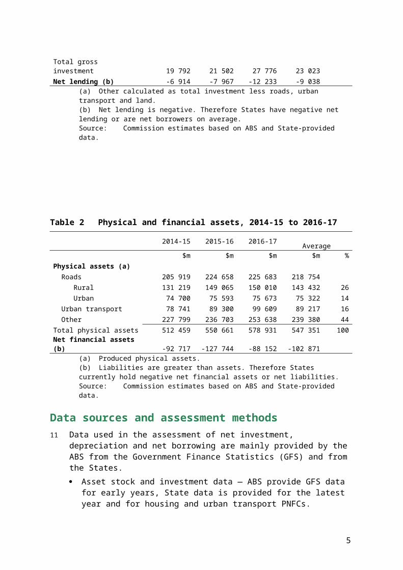
Assessed Net borrowing=[( K1P1 ) p i, 1−( K0P0 ) pi , 0]Where: pi,1 and pi,0 are the populations of State i at the end and the start of the year P1 and P0 are the Australian populations at the end and the start of the year K1 and K0 are the Australian total value of financial asset stocks at the end and start of the year, K0 is calculated as K1 minus net lendingCategory and component expenses10 Table 1 shows that States’ total net investment in physical assets was close to

$14 billion in 2016-17, with about half of that in urban transport. The total value of States’ physical assets, as shown in Table 2, is over half a trillion dollars.

Table 1 Investment, depreciation and net borrowing, 2014-15 to 2016-17

2014-15 2015-16 2016-17 Average

$m $m $m $m %Investment Roads 2 274 2 986 3 261 2 840 Rural 683 1 080 790 851 9 Urban 1 591 1 906 2 471 1 989 21 Urban transport 2 653 3 736 7 774 4 721 50 Other (a) 817 41 2 431 1 096 12 Land 775 1 299 332 802 8Total net investment 6 519 8 062 13 798 9 460 100Depreciation 13 273 13 440 13 978 13 564Total gross investment 19 792 21 502 27 776 23 023Net lending (b) -6 914 -7 967 -12 233 -9 038

(a) Other calculated as total investment less roads, urban transport and land. (b) Net lending is negative. Therefore States have negative net lending or are net borrowers on average. Source: Commission estimates based on ABS and State-provided data.

3

Table 2 Physical and financial assets, 2014-15 to 2016-17

2014-15 2015-16 2016-17 Average

$m $m $m $m %Physical assets (a) Roads 205 919 224 658 225 683 218 754 Rural 131 219 149 065 150 010 143 432 26 Urban 74 700 75 593 75 673 75 322 14 Urban transport 78 741 89 300 99 609 89 217 16 Other 227 799 236 703 253 638 239 380 44Total physical assets 512 459 550 661 578 931 547 351 100Net financial assets (b) -92 717 -127 744 -88 152 -102 871

(a) Produced physical assets.(b) Liabilities are greater than assets. Therefore States currently hold negative net financial assets or net

liabilities. Source: Commission estimates based on ABS and State-provided data.

Data sources and assessment methods11 Data used in the assessment of net investment, depreciation and net borrowing are

mainly provided by the ABS from the Government Finance Statistics (GFS) and from the States. Asset stock and investment data — ABS provide GFS data for early years, State

data is provided for the latest year and for housing and urban transport PNFCs. Department of Transport and Infrastructure provides data on national network road payments.

Population data — ABS. Stock disabilities — are derived in the relevant assessment category assessments. Cost disabilities — construction cost disabilities are derived from the regional and

capital city indices from the Rawlinsons Australian Construction Handbook1. Recurrent location factors are derived in the wage and regional costs assessments.

Net investment assessment 12 Net investment expenditure is assessed in four components. Investment in roads,

urban transport and land have specific drivers and are assessed separately. Investment in all other services is assessed in the other services component.

13 For all investment components, excluding land, population growth is the primary driver of needs. As a State’s population grows it needs to invest more to maintain the average per capita level of infrastructure required to provide services.

1 Australian Construction Handbook, Rawlinsons Publishing

4

14 The level of capital per capita required by each State varies based largely on its socio-demographic profile, and this profile changes over time. These factors are also taken into account in calculating a State’s net investment needs.

15 The cost of investing in assets (other than land) is also recognised through a cost factor which reflects a State’s relative construction, wage and regional costs. Regional and capital city construction cost indices from Rawlinsons are used to derive population weighted construction cost factors. These are combined 50/50 with recurrent regional and wage factors.

16 The drivers, in addition to population and capital costs, are discussed briefly below for each component.

17 Roads. The assessment of roads net investment recognises the impact of road length, road use and bridges on the need for road infrastructure. Urban and rural roads needs are assessed separately.

18 Urban transport. The assessment of urban transport net investment recognises the impact of city size on the need for infrastructure. Urban areas with a population over 20 000 are included in the assessment as population centres with higher needs, with the assessed need for infrastructure per capita being assumed to be proportional to population. That is, a population centre of 5 million people requires twice the urban transport infrastructure per capita, and four times the total infrastructure, as a population centre of 2.5 million.

19 Other services. Net investment in services other than roads and urban transport is assessed in the other services component. Disabilities reflecting the quantity of infrastructure required to provide services are combined and applied to total infrastructure. Recurrent disabilities, adjusted to exclude elements that do not relate to infrastructure need, have been used as a proxy for infrastructure need. For example, enrolments in government schools affect infrastructure needs and are included while enrolments in private schools do not affect government infrastructure needs and are not included.

20 Land. Investment in land is assessed on an equal per capita (EPC) basis. Stocks of general government land and investment in the acquisition of land and other non-produced assets do not affect the relativities.

Depreciation 21 The depreciation assessment provides States with the capacity to meet the

depreciation expenses on their assessed infrastructure stocks assuming they applied the average depreciation rate. The disabilities relating to the quantity and cost of infrastructure required for roads and other services infrastructure are the same as those applied in the investment assessment.

5

22 The assessment does not include urban transport depreciation because those expenses are part of the net expenses covered by the urban transport assessment.

Net borrowing23 Net borrowing reflects the extent to which the States’ total outlays on service

delivery and investment in infrastructure exceed their total revenue. The Commission assesses how much each State would need to borrow if it were to finish a year with the average per capita net financial assets, assuming it began the year with the average value at that time.

24 Interstate differences in population growth rates are the only driver of differences in net borrowing recognised in this assessment. When net financial assets are negative, as is currently the case, States hold net liabilities. A State with an above average share of population growth requires less GST revenue to maintain average levels of net financial liabilities because its fast growing population dilutes the State’s net financial liabilities at a faster rate than a slow growing State, leaving it in a stronger financial position. Put another way, States with below average population growth will not be able to borrow the average per capita amount (to achieve the average per capita net financial liabilities) and so will require additional GST revenue.

GST redistribution25 In the 2018 Update, the Investment assessment redistributed $1 585 million towards

New South Wales and Victoria away from all other States. While Victoria experienced above average population growth over the assessment years, New South Wales’ above average investment needs were largely driven by the major national investment in urban transport, where New South Wales has well above average needs.

26 Depreciation redistributed $838 million towards Queensland, Western Australia, South Australia, Tasmania and the Northern Territory from New South Wales, Victoria and the ACT. This largely mirrors the pattern in recurrent expense assessments. States with above average costs of service delivery have above average capital requirements and therefore above average consumption of capital.

27 Net borrowing redistributed $185 million from New South Wales, Victoria and the ACT towards the other States. This reflects the above average population growth in these States.

6

Table 3 GST redistribution, Investment, Depreciation and Net borrowing, 2018 Update

NSW Vic Qld WA SA Tas ACT NT Redist

$m $m $m $m $m $m $m $m $mInvestment

Roads 82 153 -14 -132 -61 -25 -4 1 236

Urban transport 198 595 -338 -147 -173 -78 -25 -33 793

Other services 53 504 -74 -206 -97 -56 9 -133 566

Total Investment 332 1 252 -425 -484 -332 -159 -20 -165 1 585

Depreciation -241 -560 105 320 90 23 -37 300 838

Net borrowing -8 -182 27 70 47 22 -3 11 185Source: Commission calculation for the 2018 Update.

ISSUES AND ANALYSIS

28 Staff consider assessing capital needs directly as they arise remains an appropriate method. However, staff think some modifications could be made to the current assessment to improve equalisation outcomes and provide greater transparency.

29 In this paper, staff focus on issues relating to the broad structure of the current assessments of physical and financial assets. Issues related to category specific infrastructure disabilities are discussed more fully in the relevant staff draft assessment paper, in particular: CGC 2018-01/17-S, Roads CGC 2018-01/18-S, Transport.

Functionalising the assessment30 In the 2010 Review, when the Commission first developed the capital assessment, in

the interests of simplicity it attempted to keep investment as a single category. It did so assuming the drivers of recurrent spending were sufficiently similar to the drivers of investment spending. However, the drivers of investment for urban and rural roads and urban transport were very different from the drivers of recurrent expenditure in those categories.2 The Commission decided that this warranted splitting those elements off from the rest of the capital assessment.3 Other services was left as a residual.

2 Roads and urban transport also represent a large proportion of total net investment (average of around 80% over 2014-15 to 2016-17) and asset stocks (about 56%).

3 The decision to separately assess urban transport investment was made in the 2015 Review with the inclusion of urban transport PNFCs.

7

31 The method for assessing infrastructure need in each category is conceptually the same. The total redistribution in the roads, urban transport and other services components is influenced by: the level of stock (including the composition of that stock) — K1

the change in the level of stock (including changes in composition) — (K1 – K0)

the stock factor — δ i ,1u

the change in the stock factor — (δ i ,1u −δi ,0

u ¿.

32 However, in the case of other services, these elements are the amalgam of ten different categories. This makes it difficult to associate redistributive impacts with any particular category.

33 Staff consider moving to a functionalised assessment, where investment in every category is assessed separately, would make the assessment easier to interpret, more accessible and more transparent. The ability to identify all expenditure needs, both recurrent and investment, related to a particular category would provide a more complete view of the service provision task. While investment for each category would be calculated separately, the assessment could be presented as part of the category assessment, part of the investment assessment or included in both.

34 The stock factors for each category in the others services component are weighted together in proportion to the value of stock of assets in each category. This means that the closing stocks for the amalgamated other services component are equivalent to those in a functionalised assessment. However, while we define opening stocks as closing stocks less net investment, when we combine them in the other services component, we use the share of assets in the previous year. Therefore, differences in revaluations of assets between categories affects the assessment of investment in other services under the current approach, but would have no effect in a functionalised assessment.

35 For example, in the 2018 Update, Victoria revised down its stock of services to communities assets by $2.5 billion for 2016-17. This implied a national disinvestment of assets in this category (where the Northern Territory had very high needs) and a corresponding national investment in all other categories within Other services. This effect reduced the Northern Territory’s GST by $37 million. Under a functionalised assessment, such revaluations would have no effect on the redistribution of GST. Other than this change, the two approaches are equivalent.

8

36 The data required to make this change — stock and investment data by ABS General Purpose Classification (GPC)4 — are available from the ABS. However, in addition to data currently provided by States in an update, investment expenditure for all relevant GPCs, not just roads and urban transport, for the most recent year will also be required.

37 Staff recognise that functionalising the assessment will introduce more steps in the Investment assessment for what is essentially a matter of presentation and could be considered a more complicated approach. On the other hand, staff consider removing the need to combine ten distinct stock factors into one factor represents a significant simplification both technically and in terms of comprehension. On balance, staff consider the benefits associated with interpretation and accessibility compensate for any increase in the quantity of calculations necessary.

38 In addition to this, assessing investment on a category by category basis allows for further refinements to be made to the assessment method, which are discussed below.

Staff propose to recommend the Commission: separately assess investment in all category and component service areas.

Refining our assessment of infrastructure needs

Averaging disabilities 39 In the 2010 Review, the Commission addressed volatility concerns and recognised

States do not respond immediately to changes in State circumstances by applying a three year averaging process for the end of year and beginning of year disabilities. While reducing volatility slightly, averaging disabilities has resulted in complicating the assessment, making it more difficult to interpret results and therefore reducing transparency. Averaging disabilities also has the effect of removing the alignment where changes in disabilities offset changes in population. This issue is most pronounced, and most easily illustrated, in reference to the rural roads assessment.

4 GPC refers to the GFS classification used to classify transactions according to their government purpose (e.g. health and education). GPC will soon be replaced by classification of the functions of government – Australia (COFOG-A). For more information, see ABS, Australian System of Government Finance Statistics: Concepts, Sources and Methods, Australia, 2015.

9

40 Each State’s share of assessed rural roads is fixed, as its geographic form does not change over time. Each State’s share of investment for rural roads is therefore driven by its share of the rural road network. As States, collectively, improve the rural road network, we assume that each kilometre of road receives the same upgrade. Unlike other asset types, there is no dilution effect. The current assessment of rural roads was designed to fully offset the impact of dilution; the box below outlines the algebra.We start with our standard formula (as expressed in the box in paragraph 8 and ignoring the cost factor for simplicity)

Assessed Investment=K1P1Pi1δi1−

K0P0Pi0δi0

A State’s rural roads disability is its share of rural road length over its share of population.Ruralroad disability=δi=

Li /LPi /PWhere L is the assessed road length of State i (i=1,..,8) for any time.When we expand out the rural road disability in the standard formula we get:

(1)K 1P1Pi1

Li / LPi1/P1

−K 0

P0Pi0

Li /LPi 0/P0Which can be significantly simplified, with all population terms cancelling out:

¿ (K1−K 0 )LiL

41 Because changes in disabilities can be volatile, we smooth them by using a three year rolling average. As shown in Table 4, a disability in an assessment year (a State’s share of road length divided by its share of population) multiplied by its share of population gives its assessed share of capital stock.5 Without three-year averaging this obviously simplifies to merely represent the State’s share of road length. However if we average three consecutive years of disability, but multiply it by a single year’s share of population, the assessed share of capital stock is no longer a constant share, and can be quite volatile.

5 As Formula (1) in the box in paragraph 40 represents K i0−K i1, the formula can be rearranged to

solve for K i

K (the share of assessed stock for a State i) at the end and start of the year.

K i

K=PiP×Li /LPi /P

10

Table 4 Worked illustration of impact of averaging length, the Northern Territory

Single year disability 3-year average disability

Share of road length

Share of population Disability (a)

Assessed share of capital stock (b) Disability (c)

Assessed share of capital stock

% % % %2010-11 9.171 1.039 8.828 9.1712011-12 9.171 1.033 8.874 9.1712012-13 9.171 1.044 8.783 9.171 8.829 9.2182013-14 9.171 1.043 8.793 9.171 8.817 9.1962014-15 9.171 1.029 8.916 9.171 8.831 9.0842015-16 9.171 1.019 9.002 9.171 8.904 9.071

(a) Calculated as share of road length divided by share of population.(b) Calculated as disability multiplied by population share.(c) Calculated as the three year average of single year disabilities.Source: Commission calculation.

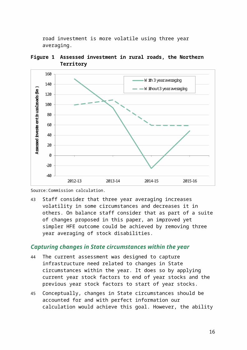
42 For a State such as the Northern Territory with volatile population growth, Figure 1 shows that the assessed rural road investment is more volatile using three year averaging.

Figure 1 Assessed investment in rural roads, the Northern Territory

-40

-20

0

20

40

60

80

100

120

140

160

2012-13 2013-14 2014-15 2015-16

Asse

ssed

inve

stm

ent i

n ur

al ro

ads (

$m)

With 3 year averaging

Without 3 year averaging

Source: Commission calculation.

43 Staff consider that three year averaging increases volatility in some circumstances and decreases it in others. On balance staff consider that as part of a suite of

11

changes proposed in this paper, an improved yet simpler HFE outcome could be achieved by removing three year averaging of stock disabilities.

Capturing changes in State circumstances within the year 44 The current assessment was designed to capture infrastructure need related to

changes in State circumstances within the year. It does so by applying current year stock factors to end of year stocks and the previous year stock factors to start of year stocks.

45 Conceptually, changes in State circumstances should be accounted for and with perfect information our calculation would achieve this goal. However, the ability to measure the change accurately is largely dependent on the capacity of the data to reliably capture the change. Taking schools as an example, in determining the level of infrastructure required to provide school services, the 2015 Review approach recognises changes in student to population ratios the socio-demographic attributes of students the cost attributed to each socio-demographic group, resulting from running the

regression on new ACARA6 data each year.

46 For each of these measures, staff consider the data provided in any given year to be the best available measure of a State’s relative need at that point in time. However, staff confidence in the capacity of these measures to accurately reflect changes over time varies from measure to measure. Staff have high confidence that variation in student to population ratios reflect real world changes, but considerably less confidence that changes in cost allocations from the regression reflect real world changes in how States fund different groups. When taking the year to year change, in addition to changes in State circumstances, the data may also incorporate changes in data collection methods and the consequences of mismatched timing of different elements contributing to the disability.

47 So, conceptually the Investment assessment should recognise observed changes in State student to population ratios and, to some extent, the socio-demographic attributes of those students. However, changes in the estimated costs for each socio-economic group should only be recognised where it is certain they reflect actual change, but not if they may reflect improvements to, or simply variation in, the cost estimates.

6 The Australian Curriculum, Assessment and Reporting Authority.

12

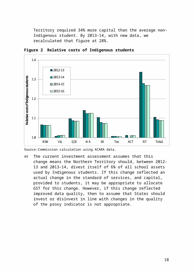
48 For example, Figure 2 shows that in 2012-13, we assessed that the average Indigenous student in the Northern Territory required 34% more capital than the average non-Indigenous student. By 2013-14, with new data, we recalculated that figure at 28%.

Figure 2 Relative costs of Indigenous students

1.0

1.1

1.2

1.3

1.4

NSW Vic Qld WA SA Tas ACT NT Total

Rela

tive

cost

of I

ndig

enou

s stu

dent

s

2012-13

2013-14

2014-15

2015-16

Source: Commission calculation using ACARA data.

49 The current investment assessment assumes that this change means the Northern Territory should, between 2012-13 and 2013-14, divest itself of 6% of all school assets used by Indigenous students. If this change reflected an actual change in the standard of services, and capital, provided to students, it may be appropriate to allocate GST for this change. However, if this change reflected improved data quality, then to assume that States should invest or disinvest in line with changes in the quality of the proxy indicator is not appropriate.

13

50 This issue is easy to identify with a hypothetical example in which the Commission had historically assessed stock need for schools EPC and then decided to improve this measure by using student numbers. Staff do not consider it would be appropriate or necessary to give all States with above average student to population ratios large amounts of GST to build schools, and to remove large amounts of GST from States with below average student to population ratios. It would be more appropriate to merely retain the implicit assumption that States start the year with the average stock per capita adjusted for their stock disabilities. This assumption allows for the actual investment requirements arising in a year to be assessed in that year.

51 Staff consider a potential solution to this issue would be to recognise the impact of service use on investment needs using a single disability and to capture the changes in circumstances that can be reliably measured in a separate disability. Staff consider the change could be captured by category specific measures of growth, as discussed in the next section.

Category specific measures of growth 52 Total population growth is currently used as a global indicator of States’ need for

investment across all categories, with States with fast growing populations assumed to have greater investment needs than States with slow growing populations. While population growth is a good proxy, a functionalised assessment would allow us to further refine this measure to capture growth in the service use populations or asset requirements of each category more specifically. For example, investment in schools is better driven by growth in government school enrolments, not growth in population. We examine this issue below in the health, schools and rural roads categories.

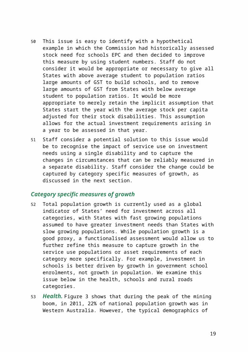
53 Health. Figure 3 shows that during the peak of the mining boom, in 2011, 22% of national population growth was in Western Australia. However, the typical demographics of people migrating to Western Australia at the time were people of prime working age. These people tend to have relatively low hospital use. The flow of people in their 70s and 80s to Western Australia was much more subdued. Therefore, Western Australia’s share of the growth in the population that typically uses hospitals was also much more subdued.

54 Over 2014 to 2015, as Western Australia’s economic growth slowed, its population aged 15 to 44 declined, while its older population continued to grow faster than the national average. So while its share of total population growth was well below average, its share of the hospital use weighted population growth was only slightly below average.

14

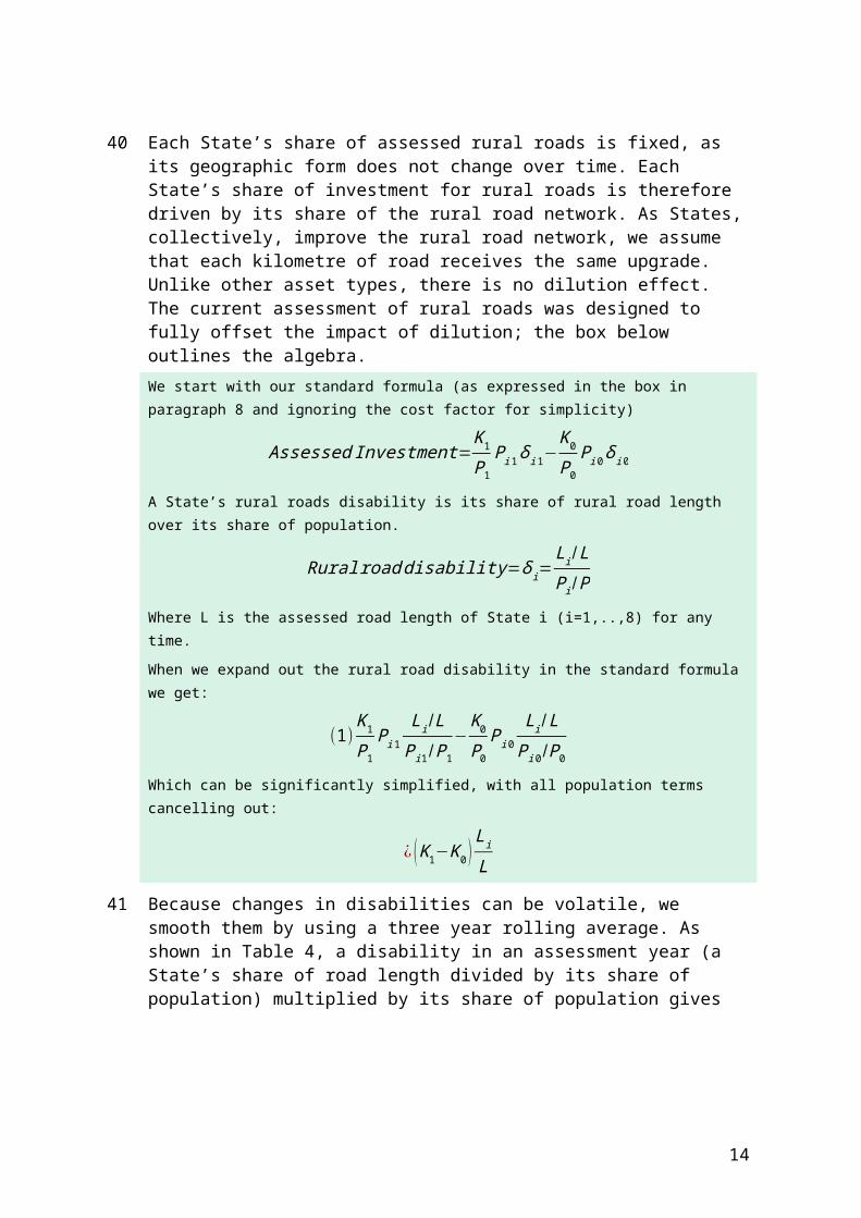
Figure 3 Western Australian share of population, growth in population and hospital user population

0

5

10

15

20

25

2000 2001 2002 2003 2004 2005 2006 2007 2008 2009 2010 2011 2012 2013 2014 2015

% o

f nati

onal

tota

l

Population growth

Weighted pop

Population

Source: Commission calculation using ABS and Independent Hospital Pricing Authority (IHPA) data.

55 Schools. Figure 4 shows that Western Australia's share of Australia's population grew until around 2013, reflecting a faster than average population growth. Since then, its share has fallen slightly. Its share of government school students has exhibited a somewhat different pattern. Between 2002 and 2011 Western Australia’s population was rapidly growing while its share of government school students was relatively stable. The reverse was true from 2013 to 2015.

15

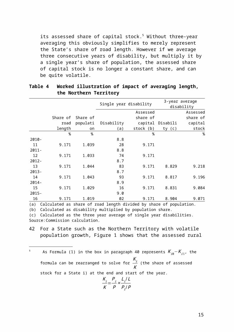
Figure 4 Growth in population and government school students, Western Australia

9.2

9.4

9.6

9.8

10.0

10.2

10.4

10.6

10.8

11.0

11.2

2002 2003 2004 2005 2006 2007 2008 2009 2010 2011 2012 2013 2014 2015 2016

% o

f nati

onal

tota

l

Population

Government school students

Source: Commission calculation using ABS and Australian Curriculum, Assessment and Reporting Authority (ACARA) data.

56 Rural roads. The current approach to rural road investment allows for dilution of the rural road stock. A State with fast population growth requires more investment per capita to retain its stock per capita. The current approach also incorporates a change in disabilities element, where fast growing States have a falling need for rural roads per capita, and therefore need less GST. These two elements were designed to offset, as discussed in the section on averaging disabilities (from paragraph 39), but due to the three year averaging approach they do not. While government school enrolments is the driver of school investment need, there is no driver of changing rural road investment need. Any investment in rural roads would be allocated between States according to their share of rural roads, not their share of change in any other indicator.

57 Changing to a category specific measure of growth makes the analysis and interpretation more appropriate. For example, as discussed from paragraph 39, if we remove three year averaging, the rural roads assessment would redistribute GST towards fast growing States, and this would be perfectly offset by a redistribution away from States with falling rural road length per capita. While the GST distribution is not changed by this, the explanation of the effect of population growth is potentially misleading.

16

58 As discussed at paragraph 44 and following, there are disabilities where the Commission has confidence in the approximate level, but not in annual change in the disability. Changing to a category specific measure of growth means that the level of these disabilities can have an appropriate effect in assessing State capital needs, but annual change in the disabilities does not.

59 Measure of service user and population growth. Introducing category based growth measures would more accurately reflect service use patterns and therefore additional infrastructure need. It would also allow for categories whose infrastructure needs are not related to population growth to use a measure that reflects actual need, for example in rural roads.

60 Under this approach it would no longer be possible to refer to population growth as the major driver of infrastructure need. Instead it would be necessary to be more specific, for example, referring to growth in service use populations such as government school students and the demographic groups that typically use hospitals.

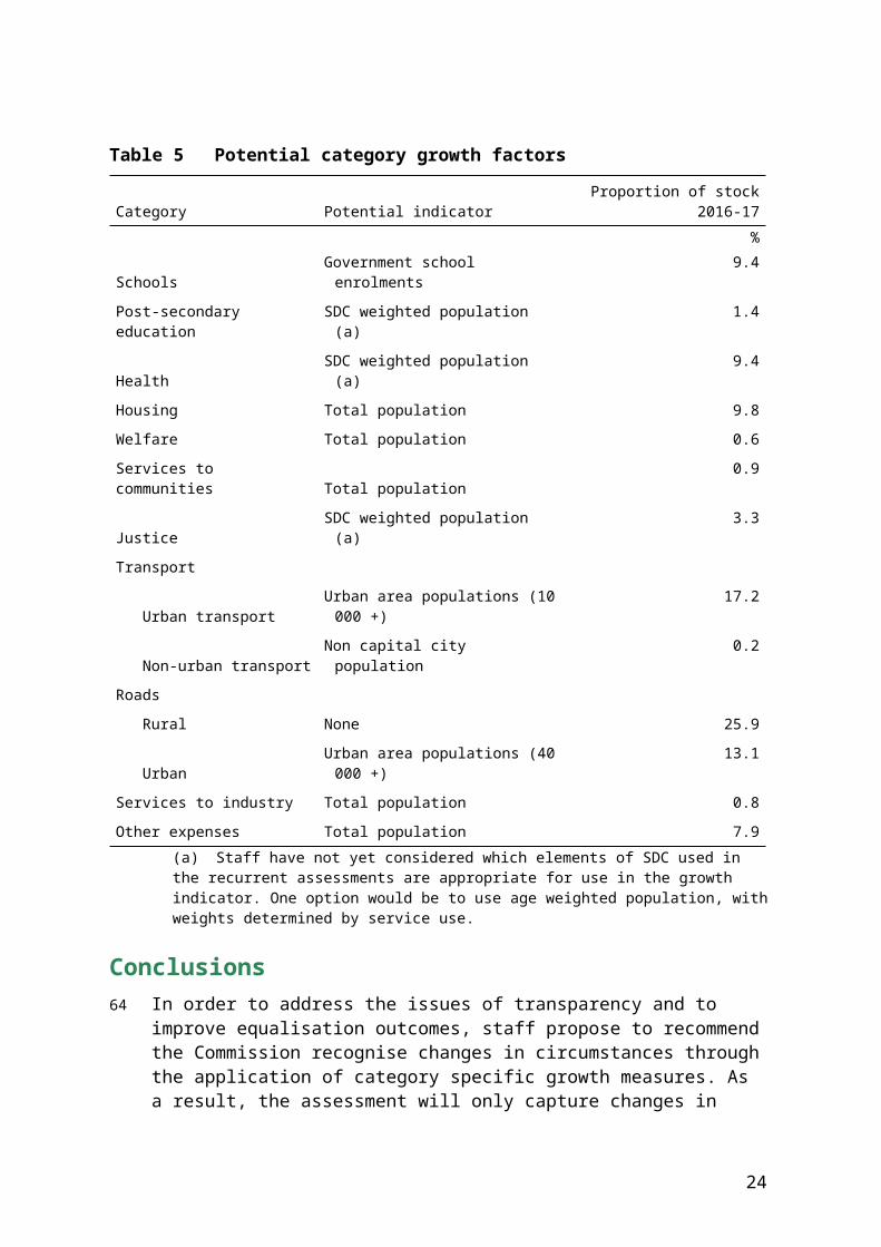
61 Staff consider reliable data and methods are available to derive category specific growth factors in a number of categories. Where data are not available or where a method cannot be derived, total population growth could be used. Table 5 lists a preliminary consideration of potential growth indicators for each category.

62 For some categories, population will remain the indicator of growth (either total population or use weighted population). In the 2018 Update, the Commission was faced with a choice of whether or not to include intercensal difference in its measure of population growth. This highlights that from time to time measures of population growth, while the best available, may incorporate measurement errors.

63 Following the 2021 Census, the ABS measure of population growth will likely incorporate an intercensal difference. Obviously the size and direction of any intercensal difference for any State cannot be known until after the 2021 Census. Staff propose to recommend the Commission establish a method of using change in population levels, incorporating any intercensal difference into its measure of population growth, in all updates using the 2020 Review methods.

17

Table 5 Potential category growth factors

Category Potential indicator Proportion of stock 2016-17

%Schools Government school enrolments 9.4

Post-secondary education SDC weighted population (a) 1.4

Health SDC weighted population (a) 9.4

Housing Total population 9.8

Welfare Total population 0.6

Services to communities Total population 0.9

Justice SDC weighted population (a) 3.3

Transport

Urban transport Urban area populations (10 000 +) 17.2

Non-urban transport Non capital city population 0.2

Roads

Rural None 25.9

Urban Urban area populations (40 000 +) 13.1

Services to industry Total population 0.8

Other expenses Total population 7.9

(a) Staff have not yet considered which elements of SDC used in the recurrent assessments are appropriate for use in the growth indicator. One option would be to use age weighted population, with weights determined by service use.

Conclusions64 In order to address the issues of transparency and to improve equalisation

outcomes, staff propose to recommend the Commission recognise changes in circumstances through the application of category specific growth measures. As a result, the assessment will only capture changes in those disabilities staff consider can be measured reliably and not those that cannot.

65 For most categories there are likely to be service use disabilities which are considered relevant to State infrastructure needs that will not be captured in the growth indicator. In order to recognise these needs, staff propose to apply the latest year’s stock disability to both opening and closing stocks.

66 For example, in schools, the growth measure would capture changes in school student numbers, and the stock disability would capture whether a State’s students needed more or less capital per student than average. We would no longer redistribute GST for the changes within the year in the socio-demographic attributes of students or changes within the year in the costs attributed to each student

18

regardless of whether it reflected unreliable data or an actual change in State priorities.

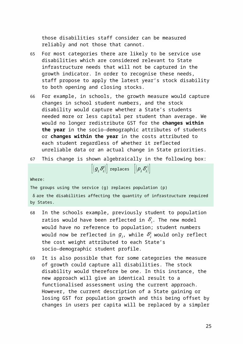
67 This change is shown algebraically in the following box:

[( gi δig )] replaces [( p i δiu ) ]Where:The groups using the service (g) replaces population (p) δ are the disabilities affecting the quantity of infrastructure required by States.68 In the schools example, previously student to population ratios would have been

reflected in δ iu. The new model would have no reference to population; student

numbers would now be reflected in gi, while δ ig would only reflect the cost weight

attributed to each State’s socio-demographic student profile.

69 It is also possible that for some categories the measure of growth could capture all disabilities. The stock disability would therefore be one. In this instance, the new approach will give an identical result to a functionalised assessment using the current approach. However, the current description of a State gaining or losing GST for population growth and this being offset by changes in users per capita will be replaced by a simpler description of whether service users are growing faster or slower than the national average.

70 For categories where a reliable growth indicator based on service use cannot be identified or where data cannot reliably support a growth indicator, population growth will continue to be used as a proxy for additional infrastructure need during the year.

71 Staff understand that by introducing category specific growth factors it will no longer be possible to refer to population growth as the global indicator of additional infrastructure need. We also understand that having multiple measures of growth could be viewed as a less simple method. However, on balance, staff consider the potential improvements to the reliability, transparency and comprehension of the assessment will make the assessment more robust, more accessible and easier to interpret. In addition, the proposal to refine the way we capture changes in State circumstances, by not including elements of the change that cannot be reliably measured, will also remove an element of volatility and the reason for three year averaging of disabilities.

19

Staff propose to recommend the Commission:

remove three year averaging of stock disabilities capture the change in circumstances through the use of category specific growth

measures, where methods can be developed and reliable data are available. If no alternative measure is available, use total population growth as a proxy where population growth is used, specify change in population levels,

rather than births, deaths and net migration, as the measure of population growth

where there are considered to be additional stock requirements not captured by the growth indicator, use the assessment year’s stock disability for both opening and closing stocks.

Other issues considered

Privately provided assets72 Smaller States may find it more difficult to attract private ownership in government

type assets compared with larger States. For example New South Wales, Victoria and Queensland have some roads built, owned and operated by the private sector. Smaller States arguably are disadvantaged in their ability to attract such investment. In the case of roads, staff consider it reflects the lack of congestion in smaller cities, and lack of demand for such assets. As such, there is no disability to assess.

73 Staff consider it would be difficult to quantify the disability faced by smaller States. and to develop an assessment of the relative need between States. Staff seek State input and data to progress this issue.

New and Old assets74 The Investment assessment assumes that a new $1 billion asset is equivalent to

holding an existing $1 billion asset. There have been various concerns raised with this assumption.

75 Costs and benefits of new capital. States own depreciated assets. For example the asset stock of schools reflects the average age of school buildings. A growing State, under our model, is given the capacity to purchase new schools for its new population at the average depreciated stock value per capita. This means it has the capacity to purchase a new depreciated asset. This is not what States do or, in most categories, can do.

76 New assets must comply with current building standards and meet community expectations both in terms of function and form. Updated methods of service delivery may demand different building methods or design. For example, the

20

increasing use of ICT in schools might lead to different classroom design and configurations. The increasing use of robot technology will require hospitals and health facilities to be built to support these new technologies.

77 How this affects the quantity and cost of the infrastructure provided is not clear to staff. While it is true that new assets may differ in structure and use to older assets previously used for the same purpose, it is also true that new capital should have greater capacity to meet State needs than capital acquired at a time when State needs, including the use of technology, were different. This could mean that States with a younger average age of assets (fast growing States) may have lower recurrent or maintenance costs.

78 Staff consider it would be difficult to quantify the costs and benefits associated with the construction of assets and to develop an assessment of the relative need between States. Staff seek State input before progressing this issue any further.

79 Under-utilisation of new assets. Because of the inefficiency of building new capital in a piecemeal way, States may choose to build new capital to cover more than one year’s growth in demand. If States build in advance of demand, then new assets will be under-utilised. Western Australia contends that this effect means that fast growing States have, on average, more under-utilised assets than slow growing States, and this represents a disability. However, States build some assets in advance of demand, and some to clear a backlog, following demand. The current approach gives all States the capacity to have average utilisation of assets over time. Staff consider this is an appropriate approach.

Treatment of Land 80 Table 6 shows the investment in land for each category in recent years. The only

category for which investment in land is large and where staff consider the appropriate disabilities are likely to be materially different from an EPC assessment is roads.

81 States spent nearly $400 million net on land purchases for road construction on average over 2013-14 to 2015-16. This was almost exclusively undertaken by the three largest States. Resuming land in cities for road construction is much more common and much more expensive in the larger cities than in the smaller cities. Some of this, and strategies such as tunnelling to avoid the requirement to resume land, is often done by private sector companies who recover these costs from motorists rather than from the general government. However governments do face significant land costs for some of this road investment. Unlike the urban transport disabilities, the urban roads disabilities do not reflect higher costs for larger cities. Staff will consider whether a proxy of need can be developed that is better than either an EPC distribution or existing disabilities.

21

Table 6 Net investment in land (a), average 2013-14 to 2015-16

Category Purchase Sales Other transactions Total

$m $m $m $mSchool education 150 -112 0 38Post-secondary education -71 -23 0 -93Health 92 -41 -10 41Housing 105 -119 5 -9Welfare 25 -9 0 16Services to communities 238 -372 -67 -201Justice 41 -10 1 32Roads 494 -109 0 385Transport (b) 40 -37 -2 1Services to industry 38 -127 -74 -164Other expenses 150 -533 -3 -386Total 1 303 -1 493 -149 -339

(a) Includes other non-produced assets.(b) Net investment in land for urban transport is not included in these data. Source: ABS, General Finance Statistics, 2013-14 to 2015-16

Net vs gross investment 82 The Commission currently recognises the use of existing infrastructure during the

year and the need for new infrastructure separately through the Depreciation and Investment assessments. For the purposes of the Commission’s assessments, depreciation is a proxy for expenditure on the replacement of existing assets.

83 The infrastructure use and cost disabilities recognised in the Investment assessment are the same as those currently used in the Depreciation assessment (with the exception of urban transport where depreciation expenses are assessed with recurrent expenses). There is a case for considering whether to assess depreciation and net investment together in a single assessment of gross investment.

84 The structure of the assessment means that changes in capital stock per capita are not subject to population dilution. Therefore, including depreciation with net investment would mean it would not be subject to population dilution. The algebra is shown in the box below.

An assessment of gross investment would combine the current assessments of net investment and depreciation (as defined in the box in paragraph 8).Investment=[( K1P1 pi ,1δ i ,1u )−( K0P0 pi , 0 δi ,0u )]δ iC

22

Depreciation= DP1p i ,1 δi , 1

u δ iC

Opening stock of capital K0 is defined as closing stock less net investment: K1−(GI−D ) , where GI is gross investment.If we replace K0 with K1−(GI−D), the full equation of both assessments becomes:

[( K1P1 pi ,1 δ i, 1u )−( K1−(GI−D)P0

pi , 0δi ,0u )]δ iC+( DP1 p i ,1δi , 1u δ iC)

This can be rearranged to:(1 )[( K1P1 pi , 1δ i ,1u )−( K1−GIP0

pi ,0 δ i ,0u )]δiC+( DP1 pi , 1δ i ,1u δiC)−( DP0 pi ,0δ i ,0u δiC)

85 The two last bracketed terms of equation (1) are very similar estimates of depreciation. If these were identical and cancelled each other out, then an assessment of gross investment would be exactly equivalent to a net assessment with an accompanying depreciation assessment.

86 However, the two depreciation terms are not identical. One uses the opening population share and stock factors while the other uses the closing population share and stock factors. This difference can, in some years, be material. For example, in the 2018 Update, the Northern Territory had rapidly changing capital stock disabilities and population. Earlier in this paper, we discussed the option of using single year disabilities in the capital assessment (see paragraph 65). If this were to be adopted, the only difference would be population.

87 Gross and net assessments produce similar outcomes. Moving to an assessment of gross investment would simplify the assessments by removing moving parts. It would also arguably increase transparency, as depreciation reflects an allowance for spending, rather than actual state expenditure. This change would also dramatically reduce the confusing prospect of negative net investment that sometimes occurs in the current assessment.

88 Staff note that the calculation of a single gross investment assessment does group together a recurrent expense (depreciation) and a capital expense (net investment). This makes presentation of total recurrent expenses difficult. For presentation purposes it would be possible to split depreciation and investment, although this would remove most of the benefits of combining them.

Recurrent versus capital disabilities89 Currently stock disabilities for all categories excluding roads and urban transport are

based on recurrent disabilities. When category assessments are more settled, staff

23

will examine recurrent disabilities and determine whether they reflect asset needs adequately. At that time we will determine whether capital specific disabilities, supported by reliable data, can be developed for individual assessments, or whether recurrent disabilities remain the best available proxy for capital needs.

Effect of population growth on financial assets (net borrowing)90 The Net borrowing assessment has one single disability. It allows for the dilution of

net financial assets or liabilities through population growth. In the 2010 Review, when this assessment was first developed, the Commission adopted a 25% discount to reflect uncertainty over the coverage of disabilities and also because some concerns were expressed about data quality. This discount was reduced to 12.5% in the 2015 Review.

91 The uncertainties associated with the disabilities related to the theory put forward by some States that population growth led to advantages as well as dilution. As States are now net borrowers rather than net lenders, the effect of the discount (relative to not having a discount) is to redistribute GST towards fast growing States. While States have articulated arguments for population growth leading to revaluations of financial assets, it is hard to conceive of a disability relating to population growth leading to revaluations of financial liabilities.

92 In the 2018 Update, the effect of the discount was to redistribute $6 per capita away from the slow growing States of Tasmania and the Northern Territory. Staff do not consider an immaterial discount warranted in these circumstances. Staff consider an assessment of net financial worth should include a disability for population dilution with no adjustments or discounts.

Staff propose to recommend the Commission: not consider differential assessment of investment in land for any category other

than roads assess the suitability of recurrent disabilities in assessing capital stock needs

when assessments are further progressed consider whether to assess depreciation expenses with net investment expenses

in an assessment of gross investment continue to assess the impact of population dilution on net financial assets,

remove the 12.5% discount and not recognise any other disabilities.

24

Issues considered and settled

Cost factors93 In the 2015 Review, the Commission introduced a construction cost index to

measure capital costs. Construction cost indices published by Rawlinsons were considered reliable and comprehensive indicators of underlying differences in construction costs. However, because the indices are based on the costs associated with commonly constructed buildings, the Commission recognised they may not represent the full costs associated with constructing some State owned assets such as hospitals and roads. The indices also do not cover investment in equipment. In light of this, the Commission decided to use an average of the capital cost disabilities and the recurrent wage and regional cost factors.

94 Separate cost factors were derived for roads, urban transport and other services investment based on the relevant populations to which the components relate.

95 Staff consider the cost factors, as developed for the 2015 Review, remain the best available measure of capital costs.

Staff propose to recommend the Commission retain the 2015 Review method of assessing capital costs through a

combination of construction cost indices and recurrent cost factors.

CONCLUSION AND WAY FORWARD

96 In conclusion, staff consider the 2015 Review assessments of physical and financial assets could be refined to: simplify the assessment and improve transparency improve the accuracy of the calculations and address volatility concerns make it easier to analyse, interpret and present results.

97 Staff propose to recommend the following refinements to the Commission: assess investment on a category by category basis apply category specific growth factors to assess change in State circumstances apply the same single year stock disability to end and beginning of year stocks explore the trade-offs of incorporating depreciation and net investment

expenditure into a single assessment of physical assets.

98 Input from States is sought prior to determining whether disabilities exist in relation to the valuation of assets and whether a reliable assessment method can be developed.

25

99 Staff propose to recommend the Commission continue to assess the impact of population growth on net financial assets with no discount or adjustment to reflect other potential disabilities.

Potential assessment structure 100 A proposed approach to assessing physical and financial assets would be applied via

assessments of: gross investment in new and replacement physical assets in each category net borrowing (or lending) to change holdings of net financial assets.

101 Collectively, the assessments would provide States with the capacity to: invest in additional physical assets to provide the new relevant user population

group added through the year with the same per user stock the existing user population had at the start of the year at the capital intensity of that State’s user population

invest in physical assets to ensure new and existing populations receive the increase in assets brought about by a national increase in capital intensity and the quality of capital (capital deepening) during the year

acquire new financial assets (or new financial liabilities if States are collectively in a net financial liability position) to provide the new population with the same per capita financial assets (liabilities) the existing population had at the start of the year (this ensures net financial assets per capita remain equal to national average net financial assets per capita).

102 The box below shows the algebraic expression for an assessment of gross investment in physical assets.

Assessed Investment=[( K1g1 gi ,1δi , 1g )−( K0g0 gi , 0δi ,1g )]δicThis is expressed in the same form as the current algebra. However, using closing year disabilities means it can be simplified to:

¿( K1g1 gi , 1−K 0

g0gi ,0)δi , 1g δ ic

This follows the same definitions as the current equation (presented in the box in paragraph 8)except, while:preferred¿ the population ,grefers ¿the groupsusing the service

δ i ,1u referred¿ the category specific disabilities per capita ,

δ i ,1g refers¿ the category specific disabilities per user

K0was calculated as K1minus net investment∈the current method ,

26

K0 is calculated as K1minus grossinvestment∈the proposedmethod .

103 This assessment would be applied separately to asset stock and investment in each category. Using schools as an example, under this model: gi ,1 and gi , 0 and would represent the number of government students in State i

at the end and start of the year. δ i ,1

g would represent the extent to which a State’s students required more expensive capital than the national average, but not whether a State had more students per capita than average, at the end of the year.

K1 would represent stocks of produced school assets and K0 would be calculated as K1 less gross investment.

104 The assessment for net borrowing would remain the same as the 2015 Review method. Staff propose no discount be applied.

Presentation 105 As noted in paragraph 33, functionalising the investment assessment, with the

separate calculation of investment needs for each category, raises the prospect of whether investment in schools is best treated as part of the schools assessment, part of the investment assessment, or some combination.

106 In addition, as noted in paragraph 88 the combination of depreciation and net investment combines recurrent and capital elements of the budget. For analysis of recurrent and capital expenditures, the impact of both can be determined separately but this will negate some of the benefits of combining them.

107 While presentation options will be considered more fully when the assessments are more settled and State views have been received, staff consider it may be best to continue to assess investment separately from recurrent expenses. Given the relative size and volatile nature of investment expenditure compared with the generally stable nature of recurrent expenditure, assessing investment within the category will likely introduce volatility to the recurrent assessments and dominate redistribution in a category.

108 Because Net borrowing redistributes GST away from fast growing States7 and Investment towards fast growing States, staff consider it should remain a separate assessment.

109 We welcome States’ advice on which presentation framework would make the assessment more transparent and aid the interpretation of results.

Staff propose to recommend the Commission:

7 This relationship holds as long as State hold, on average, net financial liabilities.

27

determine the best presentation framework based on staff and State recommendations.

Data / information sought from States110 To complete a functionalised assessment including a differential assessment of land,

in addition to the current data requirements, States will be asked to provide gross investment (net investment and depreciation) by category for the latest assessment year.

111 To progress issues related to the valuation of assets staff require States to provide evidence of the presence of a disability.

28