contents · pdf file9.4 formulas for curved beams of compact cross-section loaded normal to...

iii

Contents

List of Tables vii

Preface to the Seventh Edition ix

Preface to the First Edition xi

Part 1 Introduction

Chapter 1 Introduction 3

Terminology. State Properties, Units, and Conversions. Contents.

Part 2 Facts; Principles; Methods

Chapter 2 Stress and Strain: Important Relationships 9

Stress. Strain and the Stress–Strain Relations. Stress Transformations.Strain Transformations. Tables. References.

Chapter 3 The Behavior of Bodies under Stress 35

Methods of Loading. Elasticity; Proportionality of Stress and Strain.Factors Affecting Elastic Properties. Load–Deformation Relation for a Body.Plasticity. Creep and Rupture under Long-Time Loading. Criteria of ElasticFailure and of Rupture. Fatigue. Brittle Fracture. Stress Concentration.Effect of Form and Scale on Strength; Rupture Factor. Prestressing. ElasticStability. References.

Chapter 4 Principles and Analytical Methods 63

Equations of Motion and of Equilibrium. Principle of Superposition.Principle of Reciprocal Deflections. Method of Consistent Deformations(Strain Compatibility). Principles and Methods Involving Strain Energy.Dimensional Analysis. Remarks on the Use of Formulas. References.

For more information about this title, click here

Copyri

ghted

Mate

rial

http://dx.doi.org/10.1036/007072542X

Chapter 5 Numerical Methods 73

The Finite-Difference Method. The Finite-Element Method. The Boundary-Element Method. References.

Chapter 6 Experimental Methods 81

Measurement Techniques. Electrical Resistance Strain Gages. Detection ofPlastic Yielding. Analogies. Tables. References.

Part 3 Formulas and Examples

Chapter 7 Tension, Compression, Shear, and CombinedStress 109

Bar under Axial Tension (or Compression); Common Case. Bar under AxialTension (or Compression); Special Cases. Composite Members. Trusses.Body under Pure Shear Stress. Cases of Direct Shear Loading. CombinedStress.

Chapter 8 Beams; Flexure of Straight Bars 125

Straight Beams (Common Case) Elastically Stressed. Composite Beams andBimetallic Strips. Three-Moment Equation. Rigid Frames. Beams onElastic Foundations. Deformation due to the Elasticity of Fixed Supports.Beams under Simultaneous Axial and Transverse Loading. Beams ofVariable Section. Slotted Beams. Beams of Relatively Great Depth. Beams ofRelatively Great Width. Beams with Wide Flanges; Shear Lag. Beams withVery Thin Webs. Beams Not Loaded in Plane of Symmetry. Flexural Center.Straight Uniform Beams (Common Case). Ultimate Strength. Plastic, orUltimate Strength. Design. Tables. References.

Chapter 9 Bending of Curved Beams 267

Bending in the Plane of the Curve. Deflection of Curved Beams. CircularRings and Arches. Elliptical Rings. Curved Beams Loaded Normal to Planeof Curvature. Tables. References.

Chapter 10 Torsion 381

Straight Bars of Uniform Circular Section under Pure Torsion. Bars ofNoncircular Uniform Section under Pure Torsion. Effect of End Constraint.Effect of Longitudinal Stresses. Ultimate Strength of Bars in Torsion.Torsion of Curved Bars. Helical Springs. Tables. References.

Chapter 11 Flat Plates 427

Common Case. Bending of Uniform-Thickness Plates with CircularBoundaries. Circular-Plate Deflection due to Shear. Bimetallic Plates.Nonuniform Loading of Circular Plates. Circular Plates on ElasticFoundations. Circular Plates of Variable Thickness. Disk Springs. NarrowRing under Distributed Torque about Its Axis. Bending of Uniform-Thickness Plates with Straight Boundaries. Effect of Large Deflection.Diaphragm Stresses. Plastic Analysis of Plates. Ultimate Strength. Tables.References.

iv Contents

Copyri

ghted

Mate

rial

Chapter 12 Columns and Other Compression Members 525

Columns. Common Case. Local Buckling. Strength of Latticed Columns.Eccentric Loading: Initial Curvature. Columns under CombinedCompression and Bending. Thin Plates with Stiffeners. Short Prisms underEccentric Loading. Table. References.

Chapter 13 Shells of Revolution; Pressure Vessels; Pipes 553

Circumstances and General State of Stress. Thin Shells of Revolution underDistributed Loadings Producing Membrane Stresses Only. Thin Shells ofRevolution under Concentrated or Discontinuous Loadings ProducingBending and Membrane Stresses. Thin Multielement Shells of Revolution.Thin Shells of Revolution under External Pressure. Thick Shells ofRevolution. Tables. References.

Chapter 14 Bodies in Contact Undergoing Direct Bearingand Shear Stress 689

Stress due to Pressure between Elastic Bodies. Rivets and Riveted Joints.Miscellaneous Cases. Tables. References.

Chapter 15 Elastic Stability 709

General Considerations. Buckling of Bars. Buckling of Flat and CurvedPlates. Buckling of Shells. Tables. References.

Chapter 16 Dynamic and Temperature Stresses 743

Dynamic Loading. General Conditions. Body in a Known State of Motion.Impact and Sudden Loading. Approximate Formulas. Remarks on Stressdue to Impact. Temperature Stresses. Table. References.

Chapter 17 Stress Concentration Factors 771

Static Stress and Strain Concentration Factors. Stress ConcentrationReduction Methods. Table. References.

Appendix A Properties of a Plane Area 799

Table.

Appendix B Glossary: Definitions 813

Appendix C Composite Materials 827

Composite Materials. Laminated Composite Materials. LaminatedComposite Structures.

Index 841

Contents v

Copyri

ghted

Mate

rial

vii

List of Tables

1.1 Units Appropriate to Structural Analysis 4

1.2 Common Prefixes 5

1.3 Multiplication Factors to Convert from USCU Units to SI Units 5

2.1 Material Properties 33

2.2 Transformation Matrices for Positive Rotations about an Axis 33

2.3 Transformation Equations 34

5.1 Sample Finite Element Library 76

6.1 Strain Gage Rosette Equations Applied to a Specimen of a Linear, Isotropic

Material 102

6.2 Corrections for the Transverse Sensitivity of Electrical Resistance Strain Gages 104

8.1 Shear, Moment, Slope, and Deflection Formulas for Elastic Straight Beams 189

8.2 Reaction and Deflection Formulas for In-Plane Loading of Elastic Frames 202

8.3 Numerical Values for Functions Used in Table 8.2 211

8.4 Numerical Values for Denominators Used in Table 8.2 212

8.5 Shear, Moment, Slope, and Deflection Formulas for Finite-Length Beams on

Elastic Foundations 213

8.6 Shear, Moment, Slope, and Deflection Formulas for Semi-Infinite Beams on

Elastic Foundations 221

8.7a Reaction and Deflection Coefficients for Beams under Simultaneous Axial and

Transverse Loading: Cantilever End Support 225

8.7b Reaction and Deflection Coefficients for Beams under Simultaneous Axial and

Transverse Loading: Simply Supported Ends 226

8.7c Reaction and Deflection Coefficients for Beams under Simultaneous Axial and

Transverse Loading: Left End Simply Supported, Right End Fixed 227

8.7d Reaction and Deflection Coefficients for Beams under Simultaneous Axial and

Transverse Loading: Fixed Ends 228

8.8 Shear, Moment, Slope, and Deflection Formulas for Beams under

Simultaneous Axial Compression and Transverse Loading 229

8.9 Shear, Moment, Slope, and Deflection Formulas for Beams under

Simultaneous Axial Tension and Transverse Loading 242

8.10 Beams Restrained against Horizontal Displacement at the Ends 245

8.11a Reaction and Deflection Coefficients for Tapered Beams; Moments of Inertia

Vary as ð1þ Kx=lÞn, where n ¼ 1:0 246

8.11b Reaction and Deflection Coefficients for Tapered Beams; Moments of Inertia


8.11c Reaction and Deflection Coefficients for Tapered Beams; Moments of Inertia


8.11d Reaction and Deflection Coefficients for Tapered Beams; Moments of Inertia


8.12 Position of Flexural Center Q for Different Sections 258

8.13 Collapse Loads with Plastic Hinge Locations for Straight Beams 260

9.1 Formulas for Curved Beams Subjected to Bending in the Plane of the Curve 304

9.2 Formulas for Circular Rings 313

9.3 Reaction and Deformation Formulas for Circular Arches 333

Copyright © 2002, 1989 by the McGraw-Hill Companies, Inc.

Copyri

ghted

Mate

rial

9.4 Formulas for Curved Beams of Compact Cross-Section Loaded Normal to the

Plane of Curvature 350

10.1 Formulas for Torsional Deformation and Stress 401

10.2 Formulas for Torsional Properties and Stresses in Thin-Walled Open

Cross-Sections 413

10.3 Formulas for the Elastic Deformations of Uniform Thin-Walled Open Members

under Torsional Loading 417

11.1 Numerical Values for Functions Used in Table 11.2 455

11.2 Formulas for Flat Circular Plates of Constant Thickness 457

11.3 Shear Deflections for Flat Circular Plates of Constant Thickness 500

11.4 Formulas for Flat Plates with Straight Boundaries and Constant Thickness 502

12.1 Formulas for Short Prisms Loaded Eccentrically; Stress Reversal Impossible 548

13.1 Formulas for Membrane Stresses and Deformations in Thin-Walled Pressure

Vessels 592

13.2 Shear, Moment, Slope, and Deflection Formulas for Long and Short Thin-Walled

Cylindrical Shells under Axisymmetric Loading 601

13.3 Formulas for Bending and Membrane Stresses and Deformations in Thin- Walled

Pressure Vessels 608

13.4 Formulas for Discontinuity Stresses and Deformations at the Junctions of Shells

and Plates 638

13.5 Formulas for Thick-Walled Vessels Under Internal and External Loading 683

14.1 Formulas for Stress and Strain Due to Pressure on or between Elastic Bodies 702

15.1 Formulas for Elastic Stability of Bars, Rings, and Beams 718

15.2 Formulas for Elastic Stability of Plates and Shells 730

16.1 Natural Frequencies of Vibration for Continuous Members 765

17.1 Stress Concentration Factors for Elastic Stress (Kt) 781

A.1 Properties of Sections 802

C.1 Composite Material Systems 830

viii List of Tables

Copyri

ghted

Mate

rial

ix

Preface to theSeventh Edition

The tabular format used in the fifth and sixth editions is continued in

this edition. This format has been particularly successful when imple-

menting problem solutions on a programmable calculator, or espe-

cially, a personal computer. In addition, though not required in

utilizing this book, user-friendly computer software designed to

employ the format of the tabulations contained herein are available.

The seventh edition intermixes International System of Units (SI)

and United States Customary Units (USCU) in presenting example

problems. Tabulated coefficients are in dimensionless form for conve-

nience in using either system of units. Design formulas drawn from

works published in the past remain in the system of units originally

published or quoted.

Much of the changes of the seventh edition are organizational, such

as:

j Numbering of equations, figures and tables is linked to the parti-

cular chapter where they appear. In the case of equations, the

section number is also indicated, making it convenient to locate

the equation, since section numbers are indicated at the top of each

odd-numbered page.

j In prior editions, tables were interspersed within the text of each

chapter. This made it difficult to locate a particular table and

disturbed the flow of the text presentation. In this edition, all

numbered tables are listed at the end of each chapter before the

references.

Other changes=additions included in the seventh addition are as

follows:

j Part 1 is an introduction, where Chapter 1 provides terminology

such as state properties, units and conversions, and a description of

the contents of the remaining chapters and appendices. The defini-


Copyri

ghted

Mate

rial

tions incorporated in Part 1 of the previous editions are retained in

the seventh edition, and are found in Appendix B as a glossary.

j Properties of plane areas are located in Appendix A.

j Composite material coverage is expanded, where an introductory

discussion is provided in Appendix C, which presents the nomen-

clature associated with composite materials and how available

computer software can be employed in conjunction with the tables

contained within this book.

j Stress concentrations are presented in Chapter 17.

j Part 2, Chapter 2, is completely revised, providing a more compre-

hensive and modern presentation of stress and strain transforma-

tions.

j Experimental Methods. Chapter 6, is expanded, presenting more

coverage on electrical strain gages and providing tables of equations

for commonly used strain gage rosettes.

j Correction terms for multielement shells of revolution were

presented in the sixth edition. Additional information is provided

in Chapter 13 of this edition to assist users in the application of

these corrections.

The authors wish to acknowledge and convey their appreciation to

those individuals, publishers, institutions, and corporations who have

generously given permission to use material in this and previous

editions. Special recognition goes to Barry J. Berenberg and Universal

Technical Systems, Inc. who provided the presentation on composite

materials in Appendix C, and Dr. Marietta Scanlon for her review of

this work.

Finally, the authors would especially like to thank the many dedi-

cated readers and users of Roark’s Formulas for Stress & Strain. It is

an honor and quite gratifying to correspond with the many individuals

who call attention to errors and=or convey useful and practical

suggestions to incorporate in future editions.

Warren C. Young

Richard G. Budynas

x Preface to the Seventh Edition

Copyri

ghted

Mate

rial

xi

Preface tothe First Edition

This book was written for the purpose of making available a compact,

adequate summary of the formulas, facts, and principles pertaining to

strength of materials. It is intended primarily as a reference book and

represents an attempt to meet what is believed to be a present need of

the designing engineer.

This need results from the necessity for more accurate methods of

stress analysis imposed by the trend of engineering practice. That

trend is toward greater speed and complexity of machinery, greater

size and diversity of structures, and greater economy and refinement

of design. In consequence of such developments, familiar problems, for

which approximate solutions were formerly considered adequate, are

now frequently found to require more precise treatment, and many

less familiar problems, once of academic interest only, have become of

great practical importance. The solutions and data desired are often to

be found only in advanced treatises or scattered through an extensive

literature, and the results are not always presented in such form as to

be suited to the requirements of the engineer. To bring together as

much of this material as is likely to prove generally useful and to

present it in convenient form has been the author’s aim.

The scope and management of the book are indicated by the

Contents. In Part 1 are defined all terms whose exact meaning

might otherwise not be clear. In Part 2 certain useful general princi-

ples are stated; analytical and experimental methods of stress analysis

are briefly described, and information concerning the behavior of

material under stress is given. In Part 3 the behavior of structural

elements under various conditions of loading is discussed, and exten-

sive tables of formulas for the calculation of stress, strain, and

strength are given.

Because they are not believed to serve the purpose of this book,

derivations of formulas and detailed explanations, such as are appro-

priate in a textbook, are omitted, but a sufficient number of examples


Copyri

ghted

Mate

rial

are included to illustrate the application of the various formulas and

methods. Numerous references to more detailed discussions are given,

but for the most part these are limited to sources that are generally

available and no attempt has been made to compile an exhaustive

bibliography.

That such a book as this derives almost wholly from the work of

others is self-evident, and it is the author’s hope that due acknowl-

edgment has been made of the immediate sources of all material here

presented. To the publishers and others who have generously

permitted the use of material, he wishes to express his thanks. The

helpful criticisms and suggestions of his colleagues, Professors E. R.

Maurer, M. O. Withey, J. B. Kommers, and K. F. Wendt, are gratefully

acknowledged. A considerable number of the tables of formulas have

been published from time to time in Product Engineering, and the

opportunity thus afforded for criticism and study of arrangement has

been of great advantage.

Finally, it should be said that, although every care has been taken to

avoid errors, it would be oversanguine to hope that none had escaped

detection; for any suggestions that readers may make concerning

needed corrections the author will be grateful.

Raymond J. Roark

xii Preface to the First Edition

Copyri

ghted

Mate

rial

3

Chapter

1Introduction

The widespread use of personal computers, which have the power to

solve problems solvable in the past only on mainframe computers, has

influenced the tabulated format of this book. Computer programs for

structural analysis, employing techniques such as the finite element

method, are also available for general use. These programs are very

powerful; however, in many cases, elements of structural systems can

be analyzed quite effectively independently without the need for an

elaborate finite element model. In some instances, finite element

models or programs are verified by comparing their solutions with

the results given in a book such as this. Contained within this book are

simple, accurate, and thorough tabulated formulations that can be

applied to the stress analysis of a comprehensive range of structural

components.

This chapter serves to introduce the reader to the terminology, state

property units and conversions, and contents of the book.

1.1 Terminology

Definitions of terms used throughout the book can be found in the

glossary in Appendix B.

1.2 State Properties, Units, and Conversions

The basic state properties associated with stress analysis include the

following: geometrical properties such as length, area, volume,

centroid, center of gravity, and second-area moment (area moment of

inertia); material properties such as mass density, modulus of elasti-

city, Poisson’s ratio, and thermal expansion coefficient; loading proper-

ties such as force, moment, and force distributions (e.g., force per unit

length, force per unit area, and force per unit volume); other proper-


Copyri

ghted

Mate

rial

ties associated with loading, including energy, work, and power; and

stress analysis properties such as deformation, strain, and stress.

Two basic systems of units are employed in the field of stress

analysis: SI units and USCU units.y SI units are mass-based units

using the kilogram (kg), meter (m), second (s), and Kelvin (K) or

degree Celsius (�C) as the fundamental units of mass, length, time,

and temperature, respectively. Other SI units, such as that used for

force, the Newton (kg-m=s2), are derived quantities. USCU units are

force-based units using the pound force (lbf), inch (in) or foot (ft),

second (s), and degree Fahrenheit (�F) as the fundamental units of

force, length, time, and temperature, respectively. Other USCU units,

such as that used for mass, the slug (lbf-s2=ft) or the nameless lbf-

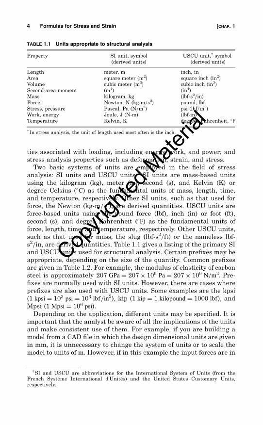
s2=in, are derived quantities. Table 1.1 gives a listing of the primary SI

and USCU units used for structural analysis. Certain prefixes may be

appropriate, depending on the size of the quantity. Common prefixes

are given in Table 1.2. For example, the modulus of elasticity of carbon

steel is approximately 207 GPa ¼ 207� 109 Pa ¼ 207� 109 N=m2. Pre-

fixes are normally used with SI units. However, there are cases where

prefixes are also used with USCU units. Some examples are the kpsi

(1 kpsi ¼ 103 psi ¼ 103 lbf=in2), kip (1 kip ¼ 1 kilopound ¼ 1000 lbf ), and

Mpsi (1 Mpsi ¼ 106 psi).

Depending on the application, different units may be specified. It is

important that the analyst be aware of all the implications of the units

and make consistent use of them. For example, if you are building a

model from a CAD file in which the design dimensional units are given

in mm, it is unnecessary to change the system of units or to scale the

model to units of m. However, if in this example the input forces are in

TABLE 1.1 Units appropriate to structural analysis

Property SI unit, symbol

(derived units)

USCU unit,y symbol

(derived units)

Length meter, m inch, in

Area square meter (m2) square inch (in2)

Volume cubic meter (m3) cubic inch (in3)

Second-area moment (m4) (in4)

Mass kilogram, kg (lbf-s2=in)Force Newton, N (kg-m=s2) pound, lbf

Stress, pressure Pascal, Pa (N=m2) psi (lbf=in2)

Work, energy Joule, J (N-m) (lbf-in)

Temperature Kelvin, K degrees Fahrenheit, �F

y In stress analysis, the unit of length used most often is the inch.

ySI and USCU are abbreviations for the International System of Units (from theFrench Systeme International d’Unites) and the United States Customary Units,respectively.

4 Formulas for Stress and Strain [CHAP. 1

Copyri

ghted

Mate

rial

Newtons, then the output stresses will be in N=mm2, which is correctly

expressed as MPa. If in this example applied moments are to be

specified, the units should be N-mm. For deflections in this example,

the modulus of elasticity E should also be specified in MPa and the

output deflections will be in mm.

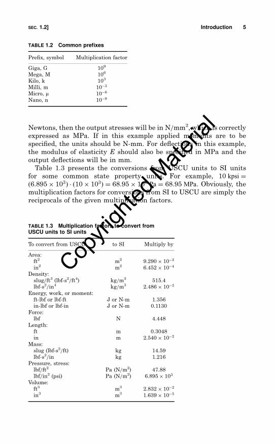
Table 1.3 presents the conversions from USCU units to SI units

for some common state property units. For example, 10 kpsi ¼ð6:895� 103Þ � ð10� 103Þ ¼ 68:95� 106 Pa ¼ 68:95 MPa. Obviously, the

multiplication factors for conversions from SI to USCU are simply the

reciprocals of the given multiplication factors.

TABLE 1.2 Common prefixes

Prefix, symbol Multiplication factor

Giga, G 109

Mega, M 106

Kilo, k 103

Milli, m 10�3

Micro, m 10�6

Nano, n 10�9

TABLE 1.3 Multiplication factors to convert fromUSCU units to SI units

To convert from USCU to SI Multiply by

Area:

ft2 m2 9:290� 10�2

in2 m2 6:452� 10�4

Density:

slug=ft3 (lbf-s2=ft4) kg=m3 515.4

lbf-s2=in4 kg=m3 2:486� 10�2

Energy, work, or moment:

ft-lbf or lbf-ft J or N-m 1.356

in-lbf or lbf-in J or N-m 0.1130

Force:

lbf N 4.448

Length:

ft m 0.3048

in m 2:540� 10�2

Mass:

slug (lbf-s2=ft) kg 14.59

lbf-s2=in kg 1.216

Pressure, stress:

lbf=ft2 Pa (N=m2) 47.88

lbf=in2 (psi) Pa (N=m2) 6:895� 103

Volume:

ft3 m3 2:832� 10�2

in3 m3 1:639� 10�5

SEC. 1.2] Introduction 5

Copyri

ghted

Mate

rial

1.3 Contents

The remaining parts of this book are as follows.

Part 2: Facts; Principles; Methods. This part describes importantrelationships associated with stress and strain, basic materialbehavior, principles and analytical methods of the mechanics ofstructural elements, and numerical and experimental techniques instress analysis.

Part 3: Formulas and Examples. This part contains the many applica-tions associated with the stress analysis of structural components.Topics include the following: direct tension, compression, shear, andcombined stresses; bending of straight and curved beams; torsion;bending of flat plates; columns and other compression members; shellsof revolution, pressure vessels, and pipes; direct bearing and shearstress; elastic stability; stress concentrations; and dynamic andtemperature stresses. Each chapter contains many tables associatedwith most conditions of geometry, loading, and boundary conditions fora given element type. The definition of each term used in a table iscompletely described in the introduction of the table.

Appendices. The first appendix deals with the properties of a planearea. The second appendix provides a glossary of the terminologyemployed in the field of stress analysis.

The references given in a particular chapter are always referred to

by number, and are listed at the end of each chapter.


Copyri

ghted

Mate

rial

9

Chapter

2Stress and Strain: Important

Relationships

Understanding the physical properties of stress and strain is a

prerequisite to utilizing the many methods and results of structural

analysis in design. This chapter provides the definitions and impor-

tant relationships of stress and strain.

2.1 Stress

Stress is simply a distributed force on an external or internal surface

of a body. To obtain a physical feeling of this idea, consider being

submerged in water at a particular depth. The ‘‘force’’ of the water one

feels at this depth is a pressure, which is a compressive stress, and not

a finite number of ‘‘concentrated’’ forces. Other types of force distribu-

tions (stress) can occur in a liquid or solid. Tensile (pulling rather than

pushing) and shear (rubbing or sliding) force distributions can also

exist.

Consider a general solid body loaded as shown in Fig. 2.1(a). Pi and

pi are applied concentrated forces and applied surface force distribu-

tions, respectively; and Ri and ri are possible support reaction force

and surface force distributions, respectively. To determine the state of

stress at point Q in the body, it is necessary to expose a surface

containing the point Q. This is done by making a planar slice, or break,

through the body intersecting the point Q. The orientation of this slice

is arbitrary, but it is generally made in a convenient plane where the

state of stress can be determined easily or where certain geometric

relations can be utilized. The first slice, illustrated in Fig. 2.1(b), is

arbitrarily oriented by the surface normal x. This establishes the yz

plane. The external forces on the remaining body are shown, as well as

the internal force (stress) distribution across the exposed internal


Copyri

ghted

Mate

rial

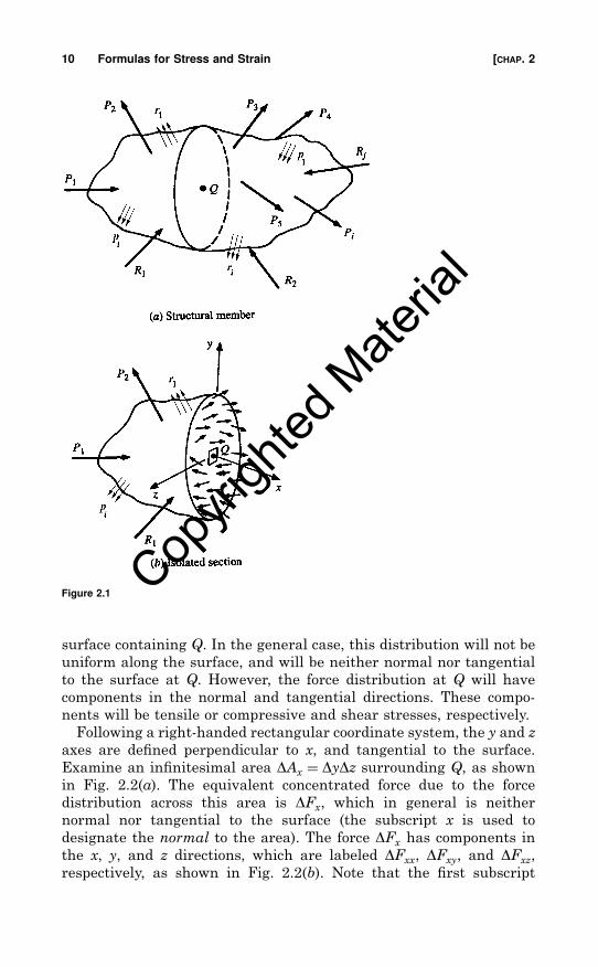
surface containing Q. In the general case, this distribution will not be

uniform along the surface, and will be neither normal nor tangential

to the surface at Q. However, the force distribution at Q will have

components in the normal and tangential directions. These compo-

nents will be tensile or compressive and shear stresses, respectively.

Following a right-handed rectangular coordinate system, the y and z

axes are defined perpendicular to x, and tangential to the surface.

Examine an infinitesimal area DAx ¼ DyDz surrounding Q, as shown

in Fig. 2.2(a). The equivalent concentrated force due to the force

distribution across this area is DFx, which in general is neither

normal nor tangential to the surface (the subscript x is used to

designate the normal to the area). The force DFx has components in

the x, y, and z directions, which are labeled DFxx, DFxy, and DFxz,

respectively, as shown in Fig. 2.2(b). Note that the first subscript

Figure 2.1


Copyri

ghted

Mate

rial

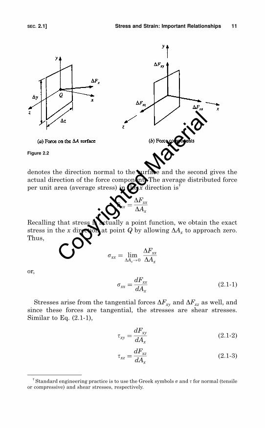
denotes the direction normal to the surface and the second gives the

actual direction of the force component. The average distributed force

per unit area (average stress) in the x direction isy

�ssxx ¼DFxx

DAx

Recalling that stress is actually a point function, we obtain the exact

stress in the x direction at point Q by allowing DAx to approach zero.

Thus,

sxx ¼ limDAx!0

DFxx

DAx

or,

sxx ¼dFxx

dAx

ð2:1-1Þ

Stresses arise from the tangential forces DFxy and DFxz as well, and

since these forces are tangential, the stresses are shear stresses.

Similar to Eq. (2.1-1),

txy ¼dFxy

dAx

ð2:1-2Þ

txz ¼dFxz

dAx

ð2:1-3Þ

Figure 2.2

yStandard engineering practice is to use the Greek symbols s and t for normal (tensileor compressive) and shear stresses, respectively.

SEC. 2.1] Stress and Strain: Important Relationships 11

Copyri

ghted

Mate

rial

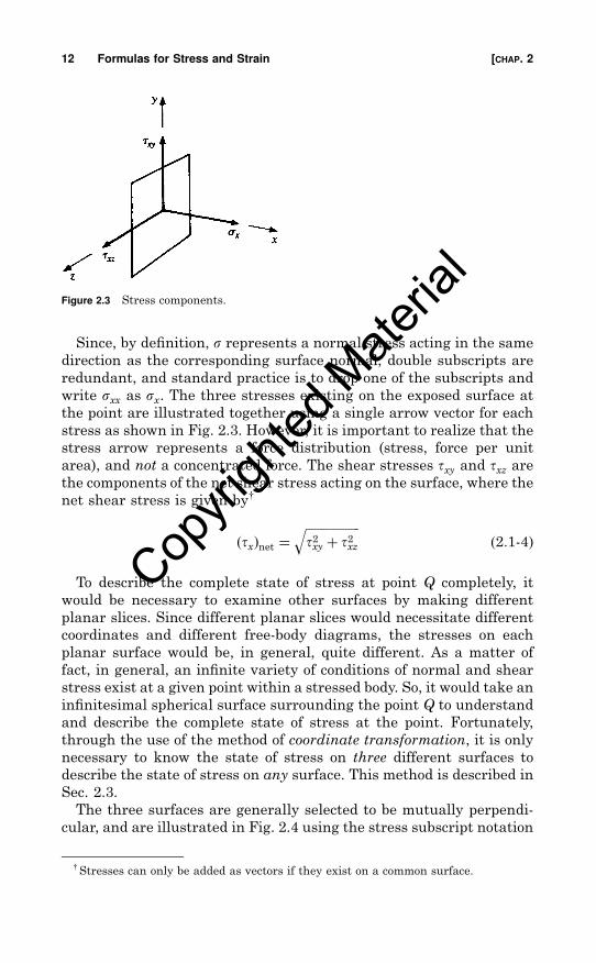
Since, by definition, s represents a normal stress acting in the same

direction as the corresponding surface normal, double subscripts are

redundant, and standard practice is to drop one of the subscripts and

write sxx as sx. The three stresses existing on the exposed surface at

the point are illustrated together using a single arrow vector for each

stress as shown in Fig. 2.3. However, it is important to realize that the

stress arrow represents a force distribution (stress, force per unit

area), and not a concentrated force. The shear stresses txy and txz arethe components of the net shear stress acting on the surface, where the

net shear stress is given byy

ðtxÞnet ¼ffiffiffiffiffiffiffiffiffiffiffiffiffiffiffiffiffiffit2xy þ t2xz

qð2:1-4Þ

To describe the complete state of stress at point Q completely, it

would be necessary to examine other surfaces by making different

planar slices. Since different planar slices would necessitate different

coordinates and different free-body diagrams, the stresses on each

planar surface would be, in general, quite different. As a matter of

fact, in general, an infinite variety of conditions of normal and shear

stress exist at a given point within a stressed body. So, it would take an

infinitesimal spherical surface surrounding the point Q to understand

and describe the complete state of stress at the point. Fortunately,

through the use of the method of coordinate transformation, it is only

necessary to know the state of stress on three different surfaces to

describe the state of stress on any surface. This method is described in

Sec. 2.3.

The three surfaces are generally selected to be mutually perpendi-

cular, and are illustrated in Fig. 2.4 using the stress subscript notation

yStresses can only be added as vectors if they exist on a common surface.

Figure 2.3 Stress components.


Copyri

ghted

Mate

rial

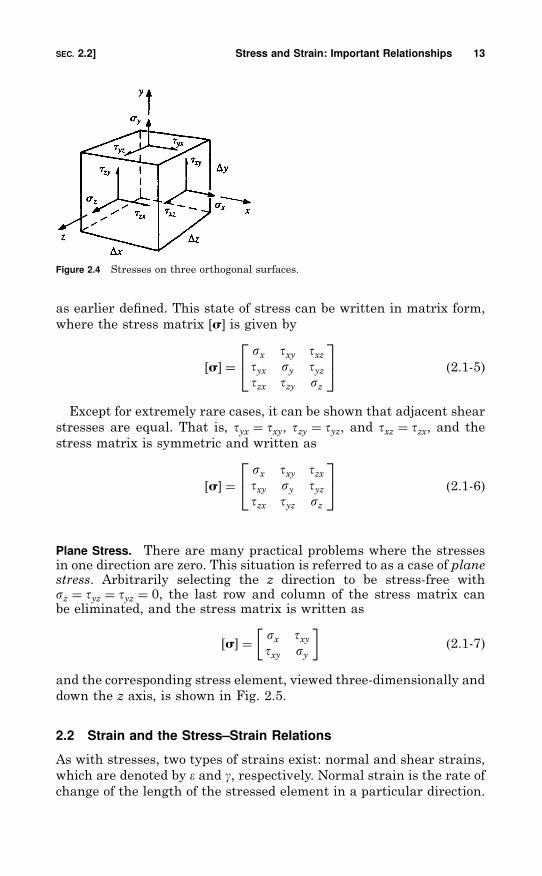
as earlier defined. This state of stress can be written in matrix form,

where the stress matrix ½s� is given by

½s� ¼sx txy txztyx sy tyztzx tzy sz

24 35 ð2:1-5Þ

Except for extremely rare cases, it can be shown that adjacent shear

stresses are equal. That is, tyx ¼ txy, tzy ¼ tyz, and txz ¼ tzx, and the

stress matrix is symmetric and written as

½s� ¼sx txy tzxtxy sy tyztzx tyz sz

24 35 ð2:1-6Þ

Plane Stress. There are many practical problems where the stressesin one direction are zero. This situation is referred to as a case of planestress. Arbitrarily selecting the z direction to be stress-free withsz ¼ tyz ¼ tyz ¼ 0, the last row and column of the stress matrix canbe eliminated, and the stress matrix is written as

½s� ¼ sx txytxy sy

� �ð2:1-7Þ

and the corresponding stress element, viewed three-dimensionally and

down the z axis, is shown in Fig. 2.5.

2.2 Strain and the Stress–Strain Relations

As with stresses, two types of strains exist: normal and shear strains,

which are denoted by e and g, respectively. Normal strain is the rate of

change of the length of the stressed element in a particular direction.

Figure 2.4 Stresses on three orthogonal surfaces.


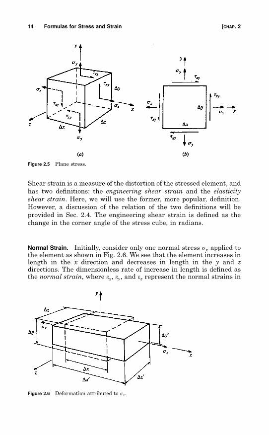
Shear strain is a measure of the distortion of the stressed element, and

has two definitions: the engineering shear strain and the elasticity

shear strain. Here, we will use the former, more popular, definition.

However, a discussion of the relation of the two definitions will be

provided in Sec. 2.4. The engineering shear strain is defined as the

change in the corner angle of the stress cube, in radians.

Normal Strain. Initially, consider only one normal stress sx applied tothe element as shown in Fig. 2.6. We see that the element increases inlength in the x direction and decreases in length in the y and zdirections. The dimensionless rate of increase in length is defined asthe normal strain, where ex, ey, and ez represent the normal strains in

Figure 2.5 Plane stress.

Figure 2.6 Deformation attributed to sx.


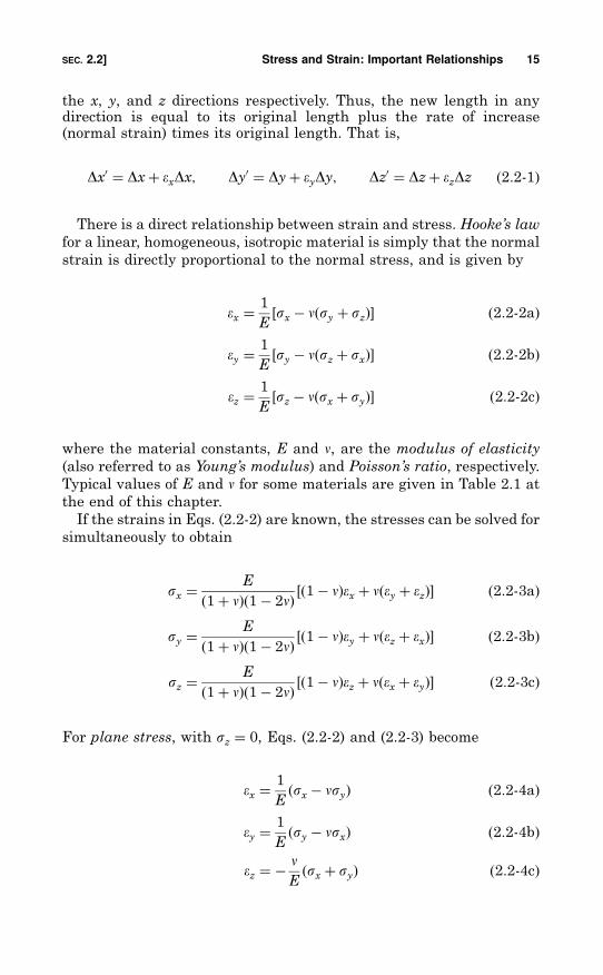
the x, y, and z directions respectively. Thus, the new length in anydirection is equal to its original length plus the rate of increase(normal strain) times its original length. That is,

Dx0 ¼ Dxþ exDx; Dy0 ¼ Dyþ eyDy; Dz0 ¼ Dzþ ezDz ð2:2-1Þ

There is a direct relationship between strain and stress. Hooke’s law

for a linear, homogeneous, isotropic material is simply that the normal

strain is directly proportional to the normal stress, and is given by

ex ¼1

E½sx � nðsy þ szÞ� ð2:2-2aÞ

ey ¼1

E½sy � nðsz þ sxÞ� ð2:2-2bÞ

ez ¼1

E½sz � nðsx þ syÞ� ð2:2-2cÞ

where the material constants, E and n, are the modulus of elasticity

(also referred to as Young’s modulus) and Poisson’s ratio, respectively.

Typical values of E and n for some materials are given in Table 2.1 at

the end of this chapter.

If the strains in Eqs. (2.2-2) are known, the stresses can be solved for

simultaneously to obtain

sx ¼E

ð1þ nÞð1� 2nÞ ½ð1� nÞex þ nðey þ ezÞ� ð2:2-3aÞ

sy ¼E

ð1þ nÞð1� 2nÞ ½ð1� nÞey þ nðez þ exÞ� ð2:2-3bÞ

sz ¼E

ð1þ nÞð1� 2nÞ ½ð1� nÞez þ nðex þ eyÞ� ð2:2-3cÞ

For plane stress, with sz ¼ 0, Eqs. (2.2-2) and (2.2-3) become

ex ¼1

Eðsx � nsyÞ ð2:2-4aÞ

ey ¼1

Eðsy � nsxÞ ð2:2-4bÞ

ez ¼ � nEðsx þ syÞ ð2:2-4cÞ


and

sx ¼E

1� n2ðex þ neyÞ ð2:2-5aÞ

sy ¼E

1� n2ðey þ nexÞ ð2:2-5bÞ

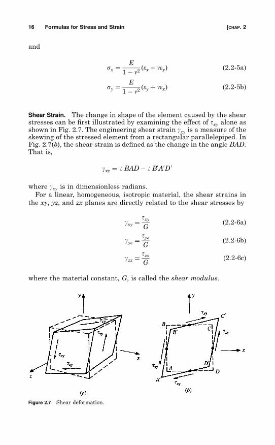
Shear Strain. The change in shape of the element caused by the shearstresses can be first illustrated by examining the effect of txy alone asshown in Fig. 2.7. The engineering shear strain gxy is a measure of theskewing of the stressed element from a rectangular parallelepiped. InFig. 2.7(b), the shear strain is defined as the change in the angle BAD.That is,

gxy ¼ ff BAD� ff B0A0D 0

where gxy is in dimensionless radians.

For a linear, homogeneous, isotropic material, the shear strains in

the xy, yz, and zx planes are directly related to the shear stresses by

gxy ¼txyG

ð2:2-6aÞ

gyz ¼tyzG

ð2:2-6bÞ

gzx ¼tzxG

ð2:2-6cÞ

where the material constant, G, is called the shear modulus.

Figure 2.7 Shear deformation.


It can be shown that for a linear, homogeneous, isotropic material

the shear modulus is related to Poisson’s ratio by (Ref. 1)

G ¼ E

2ð1þ nÞ ð2:2-7Þ

2.3 Stress Transformations

As was stated in Sec. 2.1, knowing the state of stress on three

mutually orthogonal surfaces at a point in a structure is sufficient to

generate the state of stress for any surface at the point. This is

accomplished through the use of coordinate transformations. The

development of the transformation equations is quite lengthy and is

not provided here (see Ref. 1). Consider the element shown in Fig.

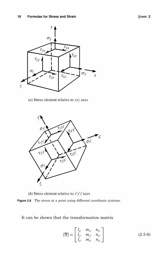
2.8(a), where the stresses on surfaces with normals in the x, y, and z

directions are known and are represented by the stress matrix

½s�xyz ¼sx txy tzxtxy sy tyztzx tyz sz

24 35 ð2:3-1Þ

Now consider the element, shown in Fig. 2.8(b), to correspond to the

state of stress at the same point but defined relative to a different set of

surfaces with normals in the x0, y0, and z0 directions. The stress matrix

corresponding to this element is given by

½s�x0y0z0 ¼sx0 tx0y0 tz0x0tx0y0 sy0 ty0z0tz0x0 ty0z0 sz0

24 35 ð2:3-2Þ

To determine ½s�x0y0z0 by coordinate transformation, we need to

establish the relationship between the x0y0z0 and the xyz coordinate

systems. This is normally done using directional cosines. First, let us

consider the relationship between the x0 axis and the xyz coordinate

system. The orientation of the x0 axis can be established by the angles

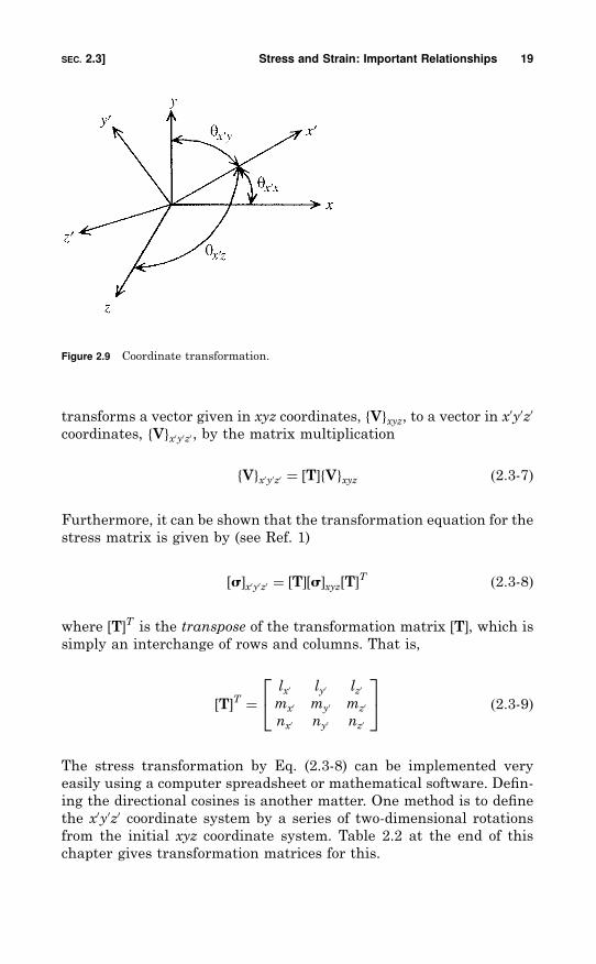
yx0x, yx0y, and yx0z, as shown in Fig. 2.9. The directional cosines for x0 aregiven by

lx0 ¼ cos yx0x; mx0 ¼ cos yx0y; nx0 ¼ cos yx0z ð2:3-3Þ

Similarly, the y0 and z0 axes can be defined by the angles yy0x, yy0y, yy0zand yz0x, yz0y, yz0z, respectively, with corresponding directional cosines

ly0 ¼ cos yy0x; my0 ¼ cos yy0y; ny0 ¼ cos yy0z ð2:3-4Þlz0 ¼ cos yz0x; mz0 ¼ cos yz0y; nz0 ¼ cos yz0z ð2:3-5Þ


It can be shown that the transformation matrix

½T� ¼lx0 mx0 nx0

ly0 my0 ny0

lz0 mz0 nz0

24 35 ð2:3-6Þ

Figure 2.8 The stress at a point using different coordinate systems.


transforms a vector given in xyz coordinates, fVgxyz, to a vector in x0y0z0

coordinates, fVgx0y0z0 , by the matrix multiplication

fVgx0y0z0 ¼ ½T�fVgxyz ð2:3-7Þ

Furthermore, it can be shown that the transformation equation for the

stress matrix is given by (see Ref. 1)

½s�x0y0z0 ¼ ½T�½s�xyz½T�T ð2:3-8Þ

where ½T�T is the transpose of the transformation matrix ½T�, which is

simply an interchange of rows and columns. That is,

½T�T ¼lx0 ly0 lz0mx0 my0 mz0

nx0 ny0 nz0

24 35 ð2:3-9Þ

The stress transformation by Eq. (2.3-8) can be implemented very

easily using a computer spreadsheet or mathematical software. Defin-

ing the directional cosines is another matter. One method is to define

the x0y0z0 coordinate system by a series of two-dimensional rotations

from the initial xyz coordinate system. Table 2.2 at the end of this

chapter gives transformation matrices for this.

Figure 2.9 Coordinate transformation.


EXAMPLE

The state of stress at a point relative to an xyz coordinate system is given bythe stress matrix

½s�xyz ¼�8 6 �2

6 4 2

�2 2 �5

24 35 MPa

Determine the state of stress on an element that is oriented by first rotatingthe xyz axes 45� about the z axis, and then rotating the resulting axes 30�about the new x axis.

Solution. The surface normals can be found by a series of coordinatetransformations for each rotation. From Fig. 2.10(a), the vector componentsfor the first rotation can be represented by

x1y1z1

8<:9=; ¼

cos y sin y 0

� sin y cos y 0

0 0 1

24 35 x

y

z

8<:9=; ðaÞ

The last rotation establishes the x0y0z0 coordinates as shown in Fig. 2.10(b), andthey are related to the x1y1z1 coordinates by

x0

y0

z0

8<:9=; ¼

1 0 0

0 cosj sinj0 � sinj cosj

24 35 x1y1z1

8<:9=; ðbÞ

Substituting Eq. (a) in (b) gives

x0

y0

z0

8><>:9>=>; ¼

1 0 0

0 cosj sinj

0 � sinj cosj

264375 cos y sin y 0

� sin y cos y 0

0 0 1

264375 x

y

z

8><>:9>=>;

¼cos y sin y 0

� sin y cosj cos y cosj sinj

sin y sinj � cos y sinj cosj

264375 x

y

z

8><>:9>=>; ðcÞ

Figure 2.10


Equation (c) is of the form of Eq. (2.3-7). Thus, the transformation matrix is

½T� ¼cos y sin y 0

� sin y cosj cos y cosj sinjsin y sinj � cos y sinj cosj

24 35 ðdÞ

Substituting y ¼ 45� and j ¼ 30� gives

½T� ¼ 1

4

2ffiffiffi2

p2

ffiffiffi2

p0

� ffiffiffi6

p ffiffiffi6

p2ffiffiffi

2p � ffiffiffi

2p

2ffiffiffi3

p

264375 ðeÞ

The transpose of ½T� is

½T�T ¼ 1

4

2ffiffiffi2

p � ffiffiffi6

p ffiffiffi2

p

2ffiffiffi2

p ffiffiffi6

p � ffiffiffi2

p

0 2 2ffiffiffi3

p

264375 ð f Þ

From Eq. (2.3-8),

½s�x0y0z0 ¼1

4

2ffiffiffi2

p2

ffiffiffi2

p0

� ffiffiffi6

p ffiffiffi6

p2ffiffiffi

2p � ffiffiffi

2p

2ffiffiffi3

p

264375 �8 6 �2

6 4 2

�2 2 �5

264375 1

4

2ffiffiffi2

p � ffiffiffi6

p ffiffiffi2

p

2ffiffiffi2

p ffiffiffi6

p � ffiffiffi2

p

0 2 2ffiffiffi3

p

264375

This matrix multiplication can be performed simply using either a computerspreadsheet or mathematical software, resulting in

½s�x0y0z0 ¼4 5:196 �3

5:196 �4:801 2:714�3 2:714 �8:199

24 35 MPa

Stresses on a Single Surface. If one was concerned about the state ofstress on one particular surface, a complete stress transformationwould be unnecessary. Let the directional cosines for the normal ofthe surface be given by l, m, and n. It can be shown that the normalstress on the surface is given by

s ¼ sxl2 þ sym

2 þ szn2 þ 2txylmþ 2tyzmnþ 2tzxnl ð2:3-10Þ

and the net shear stress on the surface is

t ¼ ½ðsxlþ txymþ tzxnÞ2 þ ðtxylþ symþ tyznÞ2

þ ðtzxlþ tyzmþ sznÞ2 � s2�1=2 ð2:3-11Þ


The direction of t is established by the directional cosines

lt ¼1

t½ðsx � sÞlþ txymþ tzxn�

mt ¼1

t½txylþ ðsy � sÞmþ tyzn� ð2:3-12Þ

nt ¼1

t½tzxlþ tyzmþ ðsz � sÞn�

EXAMPLE

The state of stress at a particular point relative to the xyz coordinate system is

½s�xyz ¼14 7 �7

7 10 0

�7 0 35

24 35 kpsi

Determine the normal and shear stress on a surface at the point where thesurface is parallel to the plane given by the equation

2x� yþ 3z ¼ 9

Solution. The normal to the surface is established by the directionalnumbers of the plane and are simply the coefficients of x, y, and z terms ofthe equation of the plane. Thus, the directional numbers are 2, �1, and 3. Thedirectional cosines of the normal to the surface are simply the normalizedvalues of the directional numbers, which are the directional numbers divided

by

ffiffiffiffiffiffiffiffiffiffiffiffiffiffiffiffiffiffiffiffiffiffiffiffiffiffiffiffiffiffiffiffiffi22 þ ð�1Þ2 þ 32

q¼ ffiffiffiffiffiffi

14p

. Thus

l ¼ 2=ffiffiffiffiffiffi14

p; m ¼ �1=

ffiffiffiffiffiffi14

p; n ¼ 3=


p

From the stress matrix, sx ¼ 14, txy ¼ 7, tzx ¼ �7, sy ¼ 10, tyz ¼ 0, and sz¼ 35kpsi. Substituting the stresses and directional cosines into Eq. (2.3-10)gives

s ¼ 14ð2=ffiffiffiffiffiffi14

pÞ2 þ 10ð�1=


pÞ2 þ 35ð3=


pÞ2 þ 2ð7Þð2=


pÞð�1=


pÞ

þ 2ð0Þð�1=ffiffiffiffiffiffi14

pÞð3=


pÞ þ 2ð�7Þð3=


pÞð2=


pÞ ¼ 19:21 kpsi

The shear stress is determined from Eq. (2.3-11), and is

t ¼ f½14ð2=ffiffiffiffiffiffi14

pÞ þ 7ð�1=


pÞ þ ð�7Þð3=


pÞ�2

þ ½7ð2=ffiffiffiffiffiffi14

pÞ þ 10ð�1=


pÞ þ ð0Þð3=


pÞ�2

þ ½ð�7Þð2=ffiffiffiffiffiffi14

pÞ þ ð0Þð�1=


pÞ þ 35ð3=


pÞ�2 � ð19:21Þ2g1=2 ¼ 14:95 kpsi


From Eq. (2.3-12), the directional cosines for the direction of t are

lt ¼1

14:95½ð14� 19:21Þð2=


pÞ þ 7ð�1=


pÞ þ ð�7Þð3=


pÞ� ¼ �0:687

mt ¼1

14:95½7ð2=


pÞ þ ð10� 19:21Þð�1=


pÞ þ ð0Þð3=


pÞ� ¼ 0:415

nt ¼1

14:95½ð�7Þð2=


pÞ þ ð0Þð�1=


pÞ þ ð35� 19:21Þð3=


pÞ� ¼ 0:596

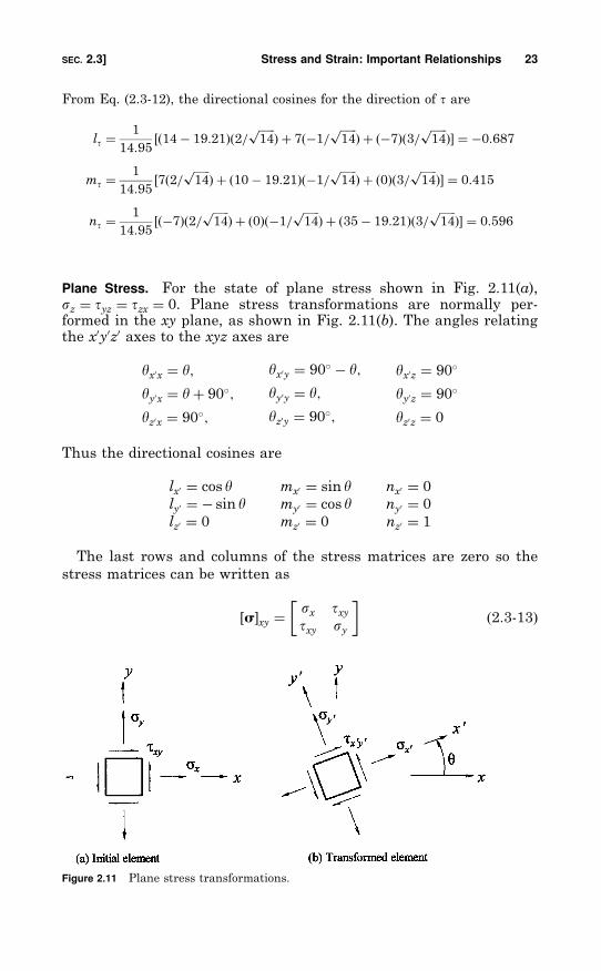
Plane Stress. For the state of plane stress shown in Fig. 2.11(a),sz ¼ tyz ¼ tzx ¼ 0. Plane stress transformations are normally per-formed in the xy plane, as shown in Fig. 2.11(b). The angles relatingthe x0y0z0 axes to the xyz axes are

yx0x ¼ y;

yy0x ¼ yþ 90�;

yz0x ¼ 90�;

yx0y ¼ 90� � y;

yy0y ¼ y;

yz0y ¼ 90�;

yx0z ¼ 90�

yy0z ¼ 90�

yz0z ¼ 0

Thus the directional cosines are

lx0 ¼ cos yly0 ¼ � sin ylz0 ¼ 0

mx0 ¼ sin ymy0 ¼ cos ymz0 ¼ 0

nx0 ¼ 0

ny0 ¼ 0

nz0 ¼ 1

The last rows and columns of the stress matrices are zero so the

stress matrices can be written as

½s�xy ¼sx txytxy sy

� �ð2:3-13Þ

Figure 2.11 Plane stress transformations.


and

½s�x0y0 ¼sx0 tx0y0tx0y0 sy0

� �ð2:3-14Þ

Since the plane stress matrices are 2� 2, the transformation matrix

and its transpose are written as

½T� ¼ cos y sin y� sin y cos y

� �; ½T�T ¼ cos y � sin y

sin y cos y

� �ð2:3-15Þ

Equations (2.3-13)–(2.3-15) can then be substituted into Eq. (2.3-8) to

perform the desired transformation. The results, written in long-hand

form, would be

sx0 ¼ sx cos2 yþ sy sin

2 yþ 2txy cos y sin y

sy0 ¼ sx sin2 yþ sy cos

2 y� 2txy cos y sin y ð2:3-16Þtx0y0 ¼ �ðsx � syÞ sin y cos yþ txyðcos2 y� sin

2 yÞ

If the state of stress is desired on a single surface with a normal

rotated y counterclockwise from the x axis, the first and third equa-

tions of Eqs. (2.3-16) can be used as given. However, using trigono-

metric identities, the equations can be written in slightly different

form. Letting s and t represent the desired normal and shear stresses

on the surface, the equations are

s ¼ sx þ sy2

þ sx � sy2

cos 2yþ txy sin 2y

t ¼ � sx � sy2

sin 2yþ txy cos 2y

ð2:3-17Þ

Equations (2.3-17) represent a set of parametric equations of a circle in

the st plane. This circle is commonly referred to as Mohr’s circle and is

generally discussed in standard mechanics of materials textbooks.

This serves primarily as a teaching tool and adds little to applications,

so it will not be represented here (see Ref. 1).

Principal Stresses. In general, maximum and minimum values of thenormal stresses occur on surfaces where the shear stresses are zero.These stresses, which are actually the eigenvalues of the stressmatrix, are called the principal stresses. Three principal stressesexist, s1, s2, and s3, where they are commonly ordered as s1 5s2 5s3.


Considering the stress state given by the matrix of Eq. (2.3-1) to be

known, the principal stresses sp are related to the given stresses by

ðsx � spÞlp þ txymp þ tzxnp ¼ 0

txylp þ ðsy � spÞmp þ tyznp ¼ 0 ð2:3-18Þtzxlp þ tyzmp þ ðsz � spÞnp ¼ 0

where lp, mp, and np are the directional cosines of the normals to the

surfaces containing the principal stresses. One possible solution to

Eqs. (2.3-18) is lp ¼ mp ¼ np ¼ 0. However, this cannot occur, since

l2p þm2p þ n2

p ¼ 1 ð2:3-19Þ

To avoid the zero solution of the directional cosines of Eqs. (2.3-18), the

determinant of the coefficients of lp,mp, and np in the equation is set to

zero. This makes the solution of the directional cosines indeterminate

from Eqs. (2.3-18). Thus,

ðsx � spÞ txy tzxtxy ðsy � spÞ tyztzx tyz ðsz � spÞ

�� ¼ 0

Expanding the determinant yields

s3p � ðsx þ sy þ szÞs2p þ ðsxsy þ sysz þ szsx � t2xy � t2yz � t2zxÞsp� ðsxsysz þ 2txytyztzx � sxt

2yz � syt

2zx � szt

2xyÞ ¼ 0 ð2:3-20Þ

where Eq. (2.3-20) is a cubic equation yielding the three principal

stresses s1, s2, and s3.To determine the directional cosines for a specific principal stress,

the stress is substituted into Eqs. (2.3-18). The three resulting equa-

tions in the unknowns lp, mp, and np will not be independent since

they were used to obtain the principal stress. Thus, only two of Eqs.

(2.3-18) can be used. However, the second-order Eq. (2.3-19) can be

used as the third equation for the three directional cosines. Instead of

solving one second-order and two linear equations simultaneously, a

simplified method is demonstrated in the following example.y

yMathematical software packages can be used quite easily to extract the eigenvalues(sp) and the corresponding eigenvectors (lp, mp, and np) of a stress matrix. The reader isurged to explore software such as Mathcad, Matlab, Maple, and Mathematica, etc.


EXAMPLE

For the following stress matrix, determine the principal stresses and thedirectional cosines associated with the normals to the surfaces of eachprincipal stress.

½s� ¼3 1 1

1 0 2

1 2 0

24 35 MPa

Solution. Substituting sx ¼ 3, txy ¼ 1, tzx ¼ 1, sy ¼ 0, tyz ¼ 2, and sz ¼ 0 intoEq. (2.3-20) gives

s2p � ð3þ 0þ 0Þs2p þ ½ð3Þð0Þ þ ð0Þð0Þ þ ð0Þð3Þ � 22 � 12 � 12�sp� ½ð3Þð0Þð0Þ þ ð2Þð2Þð1Þð1Þ � ð3Þð22Þ � ð0Þð12Þ � ð0Þð12Þ� ¼ 0

which simplifies to

s2p � 3s2p � 6sp þ 8 ¼ 0 ðaÞ

The solutions to the cubic equation are sp ¼ 4, 1, and �2MPa. Following theconventional ordering,

s1 ¼ 4 MPa; s2 ¼ 1 MPa; s3 ¼ �2 MPa

The directional cosines associated with each principal stress are determinedindependently. First, consider s1 and substitute sp ¼ 4MPa into Eqs. (2.3-18).This results in

�l1 þm1 þ n1 ¼ 0 ðbÞl1 � 4m1 þ 2n1 ¼ 0 ðcÞl1 þ 2m1 � 4n1 ¼ 0 ðdÞ

where the subscript agrees with that of s1.Equations (b), (c), and (d) are no longer independent since they were used to

determine the values of sp. Only two independent equations can be used, andin this example, any two of the above can be used. Consider Eqs. (b) and (c),which are independent. A third equation comes from Eq. (2.3-19), which isnonlinear in l1, m1, and n1. Rather than solving the three equations simulta-neously, consider the following approach.

Arbitrarily, let l1 ¼ 1 in Eqs. (b) and (c). Rearranging gives

m1 þ n1 ¼ 1

4m1 � 2n1 ¼ 1


solving these simultaneously gives m1 ¼ n1 ¼ 12. These values of l1, m1, and n1

do not satisfy Eq. (2.3-19). However, all that remains is to normalize their

values by dividing by

ffiffiffiffiffiffiffiffiffiffiffiffiffiffiffiffiffiffiffiffiffiffiffiffiffiffiffiffiffiffiffi12 þ ð1

2Þ2 þ ð1

2Þ2

q¼ ffiffiffi

6p

=2: Thus,y

l1 ¼ ð1Þð2=ffiffiffi6

pÞ ¼

ffiffiffi6

p=3

m1 ¼ ð1=2Þð2=ffiffiffi6

pÞ ¼

ffiffiffi6

p=6

n1 ¼ ð1=2Þð2=ffiffiffi6

pÞ ¼

ffiffiffi6

p=6

Repeating the same procedure for s2 ¼ 1MPa results in

l2 ¼ffiffiffi3

p=3; m2 ¼ �

ffiffiffi3

p=3; n2 ¼ �

ffiffiffi3

p=3

and for s3 ¼ �2MPa

l3 ¼ 0; m3 ¼ffiffiffi2

p=2; n3 ¼ �

ffiffiffi2

p=2

If two of the principal stresses are equal, there will exist an infinite set

of surfaces containing these principal stresses, where the normals of

these surfaces are perpendicular to the direction of the third principal

stress. If all three principal stresses are equal, a hydrostatic state of

stress exists, and regardless of orientation, all surfaces contain the

same principal stress with no shear stress.

Principal Stresses, Plane Stress. Considering the stress element shownin Fig. 2.11(a), the shear stresses on the surface with a normal in the zdirection are zero. Thus, the normal stress sz ¼ 0 is a principal stress.The directions of the remaining two principal stresses will be in the xyplane. If tx0y0 ¼ 0 in Fig. 2.11(b), then sx0 would be a principal stress, spwith lp ¼ cos y, mp ¼ sin y, and np ¼ 0. For this case, only the first twoof Eqs. (2.3-18) apply, and are

ðsx � spÞ cos yþ txy sin y ¼ 0

txy cos yþ ðsy � spÞ sin y ¼ 0ð2:3-21Þ

As before, we eliminate the trivial solution of Eqs. (2.3-21) by setting

the determinant of the coefficients of the directional cosines to zero.

That is,

ðsx � spÞ txytxy ðsy � spÞ

�� ¼ ðsx � spÞðsy � spÞ � t2xy

¼ s2p � ðsx þ syÞsp þ ðsxsy � t2xyÞ ¼ 0 ð2:3-22Þ

yThis method has one potential flaw. If l1 is actually zero, then a solution would notresult. If this happens, simply repeat the approach letting either m1 or n1 equal unity.


Equation (2.3-22) is a quadratic equation in sp for which the two

solutions are

sp ¼ 1

2ðsx þ syÞ �

ffiffiffiffiffiffiffiffiffiffiffiffiffiffiffiffiffiffiffiffiffiffiffiffiffiffiffiffiffiffiffiffiffiffiffiðsx � syÞ2 þ 4t2xy

q� �ð2:3-23Þ

Since for plane stress, one of the principal stresses (sz) is always zero,

numbering of the stresses (s1 5s2 5s3) cannot be performed until Eq.

(2.3-23) is solved.

Each solution of Eq. (2.3-23) can then be substituted into one of Eqs.

(2.3-21) to determine the direction of the principal stress. Note that if

sx ¼ sy and txy ¼ 0, then sx and sy are principal stresses and Eqs.

(2.3-21) are satisfied for all values of y. This means that all stresses in

the plane of analysis are equal and the state of stress at the point is

isotropic in the plane.

EXAMPLE

Determine the principal stresses for a case of plane stress given by the stressmatrix

½s� ¼ 5 �4

�4 11

� �kpsi

Show the element containing the principal stresses properly oriented withrespect to the initial xyz coordinate system.

Solution. From the stress matrix, sx ¼ 5, sy ¼ 11, and txy ¼ �4kpsi and Eq.(2.3-23) gives

sp ¼ 12

ð5þ 11Þ �ffiffiffiffiffiffiffiffiffiffiffiffiffiffiffiffiffiffiffiffiffiffiffiffiffiffiffiffiffiffiffiffiffiffiffiffiffiffiffiffið5� 11Þ2 þ 4ð�4Þ2

q� �¼ 13; 3 kpsi

Thus, the three principal stresses (s1;s2; s3), are (13, 3, 0) kpsi, respectively.For directions, first substitute s1 ¼ 13kpsi into either one of Eqs. (2.3-21).Using the first equation with y ¼ y1

ðsx � s1Þ cos y1 þ txy sin y1 ¼ ð5� 13Þ cos y1 þ ð�4Þ sin y1 ¼ 0

or

y1 ¼ tan�1 � 8

4

� �¼ �63:4�

Now for the other principal stress, s2 ¼ 3kpsi, the first of Eqs. (2.3-21) gives

ðsx � s2Þ cos y2 þ txy sin y2 ¼ ð5� 3Þ cos y2 þ ð�4Þ sin y2 ¼ 0

or

y2 ¼ tan�1 2

4

� �¼ 26:6�


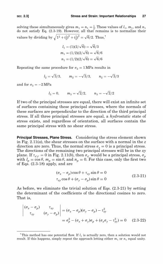
Figure 2.12(a) illustrates the initial state of stress, whereas the orientationof the element containing the in-plane principal stresses is shown in Fig.2.12(b).

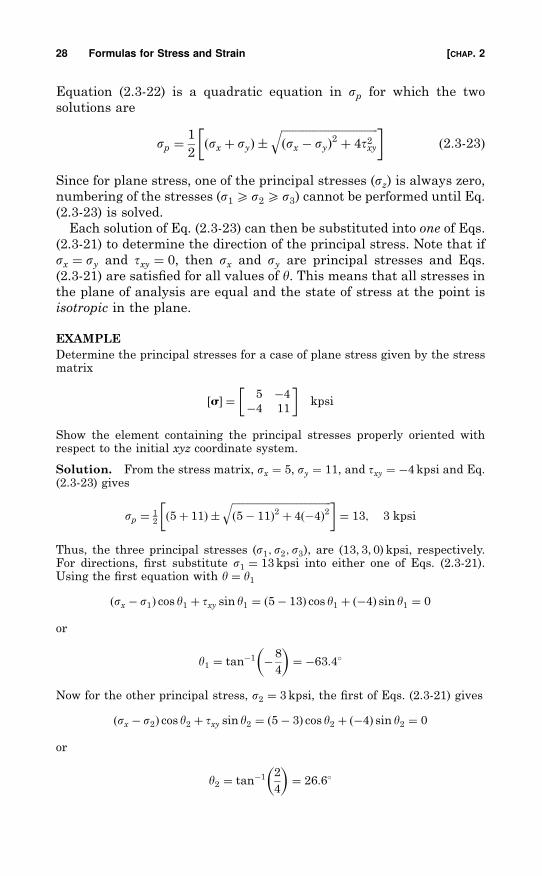
Maximum Shear Stresses. Consider that the principal stresses for ageneral stress state have been determined using the methods justdescribed and are illustrated by Fig. 2.13. The 123 axes represent thenormals for the principal surfaces with directional cosines determinedby Eqs. (2.3-18) and (2.3-19). Viewing down a principal stress axis(e.g., the 3 axis) and performing a plane stress transformation in theplane normal to that axis (e.g., the 12 plane), one would find that theshear stress is a maximum on surfaces �45� from the two principalstresses in that plane (e.g., s1, s2). On these surfaces, the maximumshear stress would be one-half the difference of the principal stresses[e.g., tmax ¼ ðs1 � s2Þ=2] and will also have a normal stress equal to theaverage of the principal stresses [e.g., save ¼ ðs1 þ s2Þ=2]. Viewingalong the three principal axes would result in three shear stress

Figure 2.12 Plane stress example.

Figure 2.13 Principal stress state.


maxima, sometimes referred to as the principal shear stresses. Thesestresses together with their accompanying normal stresses are

Plane 1; 2: ðtmaxÞ1;2 ¼ ðs1 � s2Þ=2; ðsaveÞ1;2 ¼ ðs1 þ s2Þ=2Plane 2; 3: ðtmaxÞ2;3 ¼ ðs2 � s3Þ=2; ðsaveÞ2;3 ¼ ðs2 þ s3Þ=2Plane 1; 3: ðtmaxÞ1;3 ¼ ðs1 � s3Þ=2; ðsaveÞ1;3 ¼ ðs1 þ s3Þ=2

ð2:3-24Þ

Since conventional practice is to order the principal stresses by

s1 5s2 5s3, the largest shear stress of all is given by the third of

Eqs. (2.3-24) and will be repeated here for emphasis:

tmax ¼ ðs1 � s3Þ=2 ð2:3-25Þ

EXAMPLE

In the previous example, the principal stresses for the stress matrix

½s� ¼ 5 �4

�4 11

� �kpsi

were found to be (s1; s2;s3Þ ¼ ð13; 3;0Þkpsi. The orientation of the elementcontaining the principal stresses was shown in Fig. 2.12(b), where axis 3 wasthe z axis and normal to the page. Determine the maximum shear stress andshow the orientation and complete state of stress of the element containingthis stress.

Solution. The initial element and the transformed element containing theprincipal stresses are repeated in Fig. 2.14(a) and (b), respectively. Themaximum shear stress will exist in the 1, 3 plane and is determined bysubstituting s1 ¼ 13 and s3 ¼ 0 into Eqs. (2.3-24). This results in

ðtmaxÞ1;3 ¼ ð13� 0Þ=2 ¼ 6:5 kpsi; ðsaveÞ1;3 ¼ ð13þ 0Þ=2 ¼ 6:5 kpsi

To establish the orientation of these stresses, view the element along the axiscontaining s2 ¼ 3kpsi [view A, Fig. 2.14(c)] and rotate the surfaces �45� asshown in Fig. 2.14(c).

The directional cosines associated with the surfaces are found throughsuccessive rotations. Rotating the xyz axes to the 123 axes yields

1

2

3

8><>:9>=>; ¼

cos 63:4� � sin 63:4� 0

sin 63:4� cos 63:4� 0

0 0 1

264 x

y

z

8><>:9>=>;

¼0:4472 �0:8944 0

0:8944 0:4472 0

0 0 1

264375 x

y

z

8><>:9>=>; ðaÞ


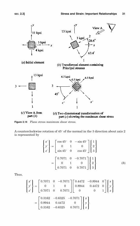
A counterclockwise rotation of 45� of the normal in the 3 direction about axis 2is represented by

x0

y0

z0

8><>:9>=>; ¼

cos 45� 0 � sin 45�

0 1 0

sin 45� 0 cos 45�

264375 1

2

3

8><>:9>=>;

¼0:7071 0 �0:7071

0 1 0

0:7071 0 0:7071

264375 1

2

3

8><>:9>=>; ðbÞ

Thus,

x0

y0

z0

8><>:9>=>; ¼

0:7071 0 �0:7071

0 1 0

0:7071 0 0:7071

264375 0:4472 �0:8944 0

0:8944 0:4472 0

0 0 1

264375 x

y

z

8><>:9>=>;

¼0:3162 �0:6325 �0:7071

0:8944 0:4472 0

0:3162 �0:6325 0:7071

264375 x

y

z

8><>:9>=>;

Figure 2.14 Plane stress maximum shear stress.


The directional cosines for Eq. (2.1-14c) are therefore

nx0x nx0y nx0zny0x ny0y ny0znz0x nz0y nz0z

24 35 ¼0:3162 �0:6325 �0:70710:8944 0:4472 0

0:3162 �0:6325 0:7071

24 35The other surface containing the maximum shear stress can be found similarlyexcept for a clockwise rotation of 45� for the second rotation.

2.4 Strain Transformations

The equations for strain transformations are identical to those for

stress transformations. However, the engineering strains as defined in

Sec. 2.2 will not transform. Transformations can be performed if the

shear strain is modified. All of the equations for the stress transforma-

tions can be employed simply by replacing s and t in the equations by eand g=2 (using the same subscripts), respectively. Thus, for example,

the equations for plane stress, Eqs. (2.3-16), can be written for strain

as

ex0 ¼ ex cos2 yþ ey sin

2 yþ gxy cos y sin y

ey0 ¼ ex sin2 yþ ey cos

2 y� gxy cos y sin y ð2:4-1Þgx0y0 ¼ �2ðex � eyÞ sin y cos yþ gxyðcos2 y� sin

2 yÞ

2.5 Reference

1. Budynas, R. G.: ‘‘Advanced Strength and Applied Stress Analysis,’’ 2nd ed., McGraw-Hill, 1999.


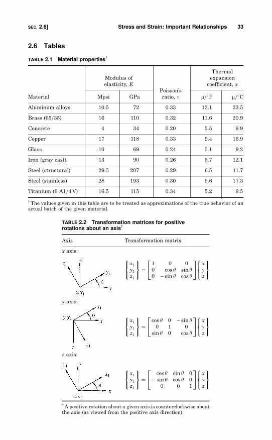
2.6 Tables

TABLE 2.1 Material propertiesy

Modulus of

elasticity, E

Thermal

expansion

coefficient, aPoisson’s

Material Mpsi GPa ratio, n m=�F m=�C

Aluminum alloys 10.5 72 0.33 13.1 23.5

Brass (65=35) 16 110 0.32 11.6 20.9

Concrete 4 34 0.20 5.5 9.9

Copper 17 118 0.33 9.4 16.9

Glass 10 69 0.24 5.1 9.2

Iron (gray cast) 13 90 0.26 6.7 12.1

Steel (structural) 29.5 207 0.29 6.5 11.7

Steel (stainless) 28 193 0.30 9.6 17.3

Titanium (6 A1=4V) 16.5 115 0.34 5.2 9.5

yThe values given in this table are to be treated as approximations of the true behavior of anactual batch of the given material.

TABLE 2.2 Transformation matrices for positiverotations about an axisy

Axis Transformation matrix

x axis:

x1y1z1

8<:9=; ¼

1 0 0

0 cos y sin y0 � sin y cos y

24 35 x

y

z

8<:9=;

y axis:

x1y1z1

8<:9=; ¼

cos y 0 � sin y0 1 0

sin y 0 cos y

24 35 x

y

z

8<:9=;

z axis:

x1y1z1

8<:9=; ¼

cos y sin y 0

� sin y cos y 0

0 0 1

24 35 x

y

z

8<:9=;

yA positive rotation about a given axis is counterclockwise aboutthe axis (as viewed from the positive axis direction).


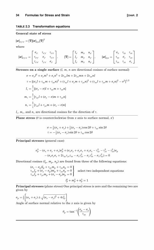
TABLE 2.3 Transformation equations

General state of stress

½s�x0y0z0 ¼ ½T�½s�xyz½T�T

where

½s�x0y0z0 ¼sx0 tx0y0 tz0x0

tx0y0 sy0 ty0z0

tz0x0 ty0z0 sz0

264375; ½T� ¼

lx0 mx0 nx0

ly0 my0 ny0

lz0 mz0 nz0

264375; ½s�xyz ¼

sx txy tzxtxy sy tyztzx tyz sz

264375

Stresses on a single surface (l, m, n are directional cosines of surface normal)

s ¼ sxl2 þ sym

2 þ szn2 þ 2txylmþ 2tyzmnþ 2tzxnl

t ¼ ½ðsxlþ txymþ tzxnÞ2 þ ðtxylþ symþ tyznÞ2 þ ðtzxlþ tyzmþ sznÞ2 � s2�1=2

lt ¼1

t½ðsx � sÞlþ txymþ tzxn�

mt ¼1

t½txylþ ðsy � sÞmþ tyzn�

nt ¼1

t½tzxlþ tyzmþ ðsz � sÞn�

lt, mt, and nt are directional cosines for the direction of t.

Plane stress (y is counterclockwise from x axis to surface normal, x0)

s ¼ 12ðsx þ syÞ þ 1

2ðsx � syÞ cos 2yþ txy sin 2y

t ¼ � 12ðsx � syÞ sin 2yþ txy cos 2y

Principal stresses (general case)

s3p � ðsx þ sy þ szÞs2p þ ðsxsy þ sysz þ szsx � t2xy � t2yz � t2zxÞsp� ðsxsysz þ 2txytyztzx � sxt

2yz � syt

2zx � szt

2xyÞ ¼ 0

Directional cosines (lp, mp, np) are found from three of the following equations:

ðsx � spÞlp þ txymp þ tzxnp ¼ 0

txylp þ ðsy � spÞmp þ tyznp ¼ 0

tzxlp þ tyzmp þ ðsz � spÞnp ¼ 0

9=; select two independent equations

l2p þm2p þ n2

p ¼ 1

Principal stresses (plane stress) One principal stress is zero and the remaining two are

given by

sp ¼ 12

ðsx þ syÞ �ffiffiffiffiffiffiffiffiffiffiffiffiffiffiffiffiffiffiffiffiffiffiffiffiffiffiffiffiffiffiffiffiffiffiffiðsx � syÞ2 þ 4t2xy

q� �Angle of surface normal relative to the x axis is given by

yp ¼ tan�1sp � sxtxy

!


841

Index

Allowable stress, 813

Alternating stress, 49

Aluminum alloys, buckling strength of,

in columns, 541

Analogies, 100, 101

electrical, for isopachic lines, 101

membrane, for torsion, 100

Analysis:

dimensional, 67

photoelastic, 84–86

Analytical methods and principles, 63–71

Apparent elastic limit, 813

Apparent stress, 813

Arches (see Circular arches; Circular

rings)

Area:

centroid of, 815

properties of, 799–801

table,802–812

Autofrettage, 587

Axial strain, 109

Axial stress, 110

Axis:

central, 815

elastic, 815

neutral (see Neutral axis)

principal, 821

Ball bearings, 689, 690

Barrel vaults, 555

Bars:

buckling of, 710

table, 718–727

lacing, 534, 535

lattice, buckling of, 535–537

Bars (Cont.):

rotating, 744, 745

torsion:

of circular, 381, 382

of noncircular , 382–389

table, 401–412

Bauschinger effect, 48

Beams, 125–263

bending moment in, 125, 814

tables, 189–201, 213–224, 229–244

bimetallic, 137–139

buckling of, 711

buckling of, 710

table, 728, 729

buckling of flange in, 182

buckling of web in, 181

change in length of, 130

composite, 137

continuous, 140

curved (see Curved beams)

deflection of:

due to bending, 125, 127

table, 189–201

due to shear, 166, 167

diagonal tension and compression in,

176, 181

on elastic foundations, 147, 148

table, 211–224

flexural center of, 177

table, 258, 259

form factors of, 181

of great depth, 166–169

of great width, 169–173

concentrated load on, 171

under impact, 752, 756–758


Beams (Cont.):

under loads not in plane of symmetry

177

neutral axis of, 177

with longitudinal slots, 165

moving loads on, 754

plastic design of, 184–188

table of collapse loads and plastic

hinge locations, 260–263

radius of curvature of, 127

resonant frequencies of, 754, 755

table, 765–768

restrained against horizontal

displacement at the ends, 155

table, 245

shear in, 129, 130, 165–167

under simultaneous axial and

transverse loading, 153–158

tables, 225–244

strain energy of, 127

stresses in, 125–130

ultimate strength of, 179

of variable section, 158–165

continuous variation, 158, 159

table, 246–257

stepped variation, 163

vertical shear in, 127

with very thin webs (Wagner beam),

175–177

with wide flanges, 173–175

Bearing stress, 689

Belleville springs, 443

Bellows:

buckling:

due to axial load, 586

due to internal pressure, 585, 717

stresses in, 634, 635

Bending:

due to torsion, 389

ultimate strength in, 179

(See also Beams; Flat plates; Shells)

Bending moment:

in beams, 814, 125

tables, 189–201, 213–224, 229–244

equivalent, 817

Bimetallic beams, 137–140

buckling of, 711

Bimetallic circular plates, 436–439

Bolts, 698

Boundary conditions, 814

Boundary element method (BEM), 73, 77

Brittle coatings, 83, 100

Brittle fracture, 814, 51

Buckling:

of arches, 711, 727

Buckling (Cont.):

of bars, 710

table, 718–727

of beam flanges, 182

of beam webs, 181

of beams, 710

table, 728, 729

of bellows, 585, 586, 717

of bimetallic beams, 711

of column flanges, 531

of column plates and webs, 533

determination of, 709

by Southwell plot, 711

due to torsion, 727

of lattice bars, 535–537

local (see Local buckling)

of plates and shells, 713

table, 730–738

of rings, 711, 727

of sandwich plates, 714

of thin plates with stiffeners, 542–544

of tubular columns, 534

Bulk modulus of elasticity, 814

formula for, 122

Bursting pressure for vessels, 588

Bursting speed of rotating disks, 751

Cable, flexible, 245

Capacitance strain gage, 84

Cassinian shells, 554

Cast iron:

general properties of, 33, 38

Castigliano’s second theorem, 66

Center:

elastic, 816

of flexure, 817

table, 802–812

of shear, 822

table, 413–416

of torsion, 824

of twist, 824

Centroid of an area, 815

table, 802–812

Centroidal axis, 815

Chafing fatigue, 818

Circular arches, 290–295

bending moments, axial and shear

forces, and deformations, table,

333–349

elastic stability of, 711

table, 727

Circular plates, 428–443, 448–450, 455–

501

bending moments, shears and

deformations, table, 333–499

842 Index

Circular plates (Cont.):


bursting speeds, 751

concentrated loads on, 428, 439

deformations due to shear, 433

table, 500, 501

dynamic stress due to rotation, 745–750

on elastic foundations, 439

elastic stability of, 714

table, 734

large deflections, effect of, 448, 449

table, 449, 450

nonuniform loading of, 439

of variable thickness, 441

vibration of, 755

resonant frequencies and mode

shapes, table, 767, 768

Circular rings, 285–290, 313–332

bending moments, axial and shear

forces, and deformations, table,

313–332

under distributed twisting couples, 444

dynamic stress due to rotation, 332, 745

elastic stability of, 711, 727

loaded normal to the plane of curvature,

297

Circumference in shells, 553

Classical laminated plate theory (CLPT),

831

Coatings, brittle, 83, 100

Collapsing pressure for tubes, 585

table, 736

Columns, 525–552

coefficient of constraint, 526

under eccentric loading, 537–540

short prisms, 544–547

table, 548–551

formulas for, 526–529

with initial curvature, 537

interaction formulas for combined

compression and bending, 540

latticed, 535

local buckling of, 529–535

in flanges, 531

in lattice bars, 535–537

in thin cylindrical tubes, 534

in thin webs, 533

long, 526

short, 527

stresses in, 529

transverse shear in, 535

Combined stresses, 121

Composite materials, 827–840

laminated, 829

material properties, table, 830

Composite members, 114, 137

Concentrated loads:

on flat plates, 428, 439

tables, 491–493, 502, 517–519

on thin shells, 610, 611, 636, 637

on wide beams, 171

Concrete:

general properties, 33, 38

under sustained stress, 40

Conical-disk spring, 443

Conical shells, 566

buckling, 715

table, 737, 738

table, 611–633

Consistent deformations, method of, 64

Contact stress, 689–707

under dynamic conditions, 693

in gear teeth, 699

in pins and bolts, 698

table, 702–704

Coordinate transformations, 17

Corrections, strain gages, 95

tables, 104, 105

Corrosion fatigue, 48, 815

Corrugated tubes, 634, 635

buckling of, 585, 717

Coulomb-Mohr theory of failure, 45

Crack initiation, 47

Crack propagation, 47

Creep, 40, 815

Criteria of failure, 41–46

Critical slenderness ratio, 526

Curve, elastic, 127, 816

Curved beams, 267–380

helical springs, 398

loaded normal to the plane of curvature:

closed circular rings, 297, 298

compact cross sections, 297

moments and deformations of,

table, 350–378

flanged sections, 302

loaded in the plane of curvature, 267–

296

circular arches, 348–350


table, 333–349

circular rings, 285–290


table, 313–332

deflection of, 275–285

with large radius of curvature, 275

with small radius of curvature, 278

with variable cross section, 283

with variable radius, 283

distortion of tubular sections, 277

Index 843

Curved beams (Cont.):

elliptical rings, 295

neutral axis of, table, 304–312

normal stress, 267

radial stress, 271

shear stress, 270

U-shaped members, 275, 794

with wide flanges, 273

Cyclic plastic flow, 47

Cylinder:

hollow, temperature stresses in, 761,

762

thin-walled, concentrated load on,

636, 637

solid, temperature stresses in, 763

Cylindrical rollers:

allowable loads on, 691

deformations and stresses, table, 703

tests on, 691

Cylindrical vessels:

thick, stresses in, 587–589

table, 683–685

thin:

bending stresses in, 557–564

table,601–607

under external pressure, 585, 716

table, 736

membrane stresses in, 554

table, 592, 593

on supports at intervals, 589–591

Damage law, linear, 51

Damaging stress, 815

Damping capacity, 815

in vibrations, 754

Deep beams, 166–169

deflections of, 167

stresses in, 168

Deflections:

of beams (see Beams, deflection of)

of diaphragms, 448, 450

of plates (see Circular plates; Flat

plates)

of trusses, 116–119

Deformation, 815

lateral, 110

torsional, table, 401–412

Diagonal tension:

field beam, 176

in thin webs, 175–177

Diaphragm, flexible, 448, 450

Diaphragm stresses (see Membrane

stresses)

Differential transformer, linear, 84

Diffraction grating strain gage, 84

Dimensional analysis, 67

Directional cosines, 17

Discontinuity stresses in shells, 572

table, 638–682

Disk:

bimetallic, 436

dynamic stresses in rotating, 745–750

temperature stresses in, 760

Disk spring, 443, 444

Dynamic loading, 36, 743–758

Dynamic stress, 744–758

Eccentric loading:

on columns, 537–540

defined, 815

on prisms, 544–547

on riveted joints, 697

Eccentric ratio for columns, 527

Effective length of columns, 526

Effective width:

of thin curved plates in compression,

543

of thin flat plates in compression,

542

of wide beams, 170

of wide flanges, 173

Elastic axis, 816

Elastic center, 816

Elastic curve, 127, 816

Elastic deformation, 815

Elastic failure, 41–46

Elastic foundations:

beams on, 147, 148

table, 211–224

plates on, 439

Elastic limit, 816

apparent, 813

Elastic ratio, 816

Elastic stability, 58, 709–742

tables, 718–738

Elastic strain energy, 823

Elastic stress, factors of stress

concentration for, table, 781–794

Elasticity, 37

modulus of, 819

Electrical analogy for isopachic lines, 101

Electrical resistance strain gage, 83, 87–

100

Electrical strain gages, 83

Ellipsoid:

of strain, 816

of stress, 816

Elliptic cylinders, 555

844 Index

Elliptical plates:

large deflections for, 451

table, 499

Elliptical rings, 295

Elliptical section in torsion, table, 401, 404

Embedded photoelastic model, 85

Endurance limit, 47, 816

Endurance ratio, 817

Endurance strength, 817

Energy:

losses in impact, 756

of rupture, 817

strain (see Strain energy)

Equation of three moments, 140

Equations of motion and equilibrium,

63

Equivalent bending moment, 817

Equivalent eccentricity for columns, 527

Equivalent radius for concentrated loads

on plates, 428

Equivalent twisting moment, 817

Euler’s column formula, 526

Experimental methods of stress

determination, 81–106

Extensometers, 82

Factor:

form, 54, 166, 181, 818

of safety, 817

of strain concentration, 823

of strength reduction, 53

of stress concentration, 53, 824

elastic, table, 781–794

at rupture, 53

Failure:

criteria of, 41–46

of wood, 45

Fatigue, 36, 46–51, 817

chafing (fretting), 818

corrosion, 48

life gage, 51

limit, 29, 817

strength, 817

Fiber stress, 126

Fillet welds, 700

Finite difference method (FDM), 73

Finite element method (FEM), 73–77

Fixed supports, 817

deformations due to the elasticity of, 152

Flange:

in beams, buckling of, 182, 710

table, 729

in columns, 531

effective width of, 173

Flat plates, 427–524

circular, 428–443, 448–450, 455–501


coefficients and formulas for, 428, 429

table, 455–499

under concentrated loading, 428, 439

table, 491–493, 502, 517–519

deflection due to shear of, 433

table, 500, 501

on elastic foundations, 439

with large deflections, 448, 449

table, 449, 450

membrane (diaphragm) stresses in,

448

under nonuniform loading, 439

perforated, 443

stability of, 713

table, 734

thermal stresses in, 484–487, 491

trunnion loading on, 493, 494

ultimate strength of, 453


elliptical, table, 499

large deflection for, 451

with straight edges, 446

coefficients for, 447

table, 502–520

with large deflections, 451

table, 452


plastic analysis of, 451, 453

stability of, 713, 714

table, 730–733

ultimate strength of, 453, 454


Flexural center, 177–179, 817

table, 258, 259

Flow, 40, 815

Flow analogy, 776

Forces, inertia, 743

Form, effect on strength of, 54

Form factor, 54, 166, 181, 818

Formulas, use of, 69, 70

Fracture, brittle, 51, 52

Frames (see Rigid frames)

Fretting fatigue, 818

Gear teeth, 168, 169, 699

contact stresses in, 699

Goodman diagram, 49

Guided boundaries, 818

Gyration, radius of, 800, 801, 822

table, 802–812

Index 845

Haigh diagram, 50

Held boundaries, 818

Helical springs, 398

Hemispherical shells, 565

table, 608–611

Hollow cylinders:

thick-walled, 699

temperature stresses in, 762, 763

thin-walled (see Cylindrical vessels,

thin)

Hollow pins, 699

Hollow rollers, 699

Hollow sphere, temperature stresses in,

763

Holographic interferometry, 86

Hooke’s law, 37

Hoop, rotating, stresses in, 332, 745

Hoop stresses (see Shells)

Hyperbolic paraboloid, 555

Hysteresis, mechanical, 818

Impact loading, 36, 752–758

Impact stresses, remarks on, 758

Inductance strain gage, 84

Inertia:

moment of (see Moment, of inertia)

product of, 800, 821

table, 802–812

rotary, 755

Inertia forces, 743

Influence line, 819

Initial curvature of columns, 537

Initial stress, 56–58

Interferometric strain gage, 84

Interferometry, 84–87

holographic, 86

laser speckle, 86

moire, 86

shadow optical method of caustics, 87

Isoclinic lines, 819

Isopachic lines, electrical analogy for,

101

Isostatic, 824

Isotropic, 819

Joints:

riveted, 695–698

welded, 700

Kern, 8, 505

shape of, table, 548–551

Keys, shear in, 700

Lacing bars, 534, 535

Laminated composite materials, 829

properties, table, 830

Laminated composite structures, 837

axially loaded, 839

in bending, 837

Large deflection of plates, 448–451

circular, 448

table, 449, 450

elliptical, 451

parallelogram, 451

rectangular, 451

table, 452

Lateral buckling of beams, 710

table, 728, 729

Lateral deformation, 110

Latticed columns, 534–537

local buckling of, 535–537

Least work, principle of, 66, 117

Limit:

elastic, 816

endurance, 47, 816

proportional, 821

Linear damage law, 51

Linear differential transformer, 84

Loading:

dynamic, 36, 743–758

eccentric (see Eccentric loading)

impact, 36, 752–758

methods of, 35

Loads:

concentrated (see Concentrated loads)

unit, method of, 65, 116

Local buckling, 529–535

of attached plates, 534

of lacing bars, 534

of latticed columns, 534

of outstanding flanges, 531

of thin cylindrical tubes, 534

of thin plates with stiffeners, 542–544

of thin webs, 181, 533

Longitudinal stress:

due to torsion, 389

and strain, 110

Luders lines (slip lines), 823

Margin of safety, 819

Material properties, table, 33

Maximum-distortional-energy theory, 42,

43

Maximum-octahedral-shear-stress theory,

42–43

Maximum-principal-strain theory, 42

Maximum-principal-stress theory, 42

846 Index

Maximum-shear-stress theory, 42, 44

Mean stress, 49

Measurement of strain, 62–87

Mechanical hysteresis, 9

Mechanical lever extensometer, 82

Membrane analogy for torsion, 100

Membrane stresses:

in flat plates, 448

in pressure vessels, 554, 555, 557

table, 592–600

Meridian in shells, 553

Methods:

analytical, 63–71

experimental, 81–106

numerical, 73–79

Mode shapes:

in vibrating beams, 754

table, 765, 766

in vibrating plates, 755

table, 767, 768

Modulus:

bulk, 814

formula for, 122

of elasticity, 15, 819

of resilience, 820

of rigidity (shear modulus), 16, 820

of rupture:

in bending, 179, 820

in torsion, 398, 820

section, 129, 822

Moire techniques, 86

Moment:

of area, 820

bending (see Bending moment)

of inertia:

of an area, 799–801, 820

table, 802–812

of composite sections, 137

polar, 381, 800, 821

equivalent constant, 383

tables, 401–416

principal, 800, 821

Motion, equations of, 63

Moving loads on beam, 754

Multielement shells of revolution,

572–585

stresses and deformations, table,

638–682

Multilayer vessel, 587

Narrow ring under distributed torque, 444

Neuber’s formula, 774

Neutral axis, 127, 820

Neutral axis (Cont.):

of beams loaded in plane of symmetry

(centroidal axis), table, 802–812

of beams not loaded in plane of

symmetry, 177

of curved beams, table, 304–312

of prisms eccentrically loaded, table,

548–551

Neutral surface, 125, 820

Notch sensitivity, 53

Notch-sensitivity ratio, 820

Numerical methods, 73–79

the boundary element method, 77

the finite difference method, 73

the finite element method, 74

Ogival shells, 554

Omega joint, 634

Optical-lever extensometer, 82

Optical remote sensing, 82

Orthotropic plates, 453

Parabolic formula for columns, 528

Parallel-axes theorem, 800

Parallelogram plates:

bending of, 447

table, 518, 519

buckling of, 714, 733

large deflection of, 451

Perforated plates, 443

Photoelastic analysis:

three-dimensional, 85

scattered light, 85

by stress freezing, 85

two-dimensional, 84

Photoelastic coatings, 85, 86

Pins, 698

hollow, 699

Pipes, 553

circumferential bending in, table, 327,

331

supported at intervals, 589–591

Plane area, properties of, 799–801

table, 802–812

Plastic analysis:

beams, 184–188

section modulus for, 180, 185, 801, 821

shape factor for, 181

table of collapse loads and plastic

hinge locations, 260–263

plates, 451, 453

Plastic flow, 40, 815

Plastic moment, 180, 821

Plasticity, 39, 821

Index 847

Plastics:

creep of, 40

used in photoelasticity, 85

Plate girders, stiffeners for, 182

Plates (see Flat plates; Large deflection of

plates)

Poisson’s ratio, 15, 121, 821

Polar moment of inertia, 381, 800, 821

equivalent constant, 383

tables, 401–416

Pressure, collapsing, for tubes, 585

table, 736

Pressure vessels (see Shells)

Prestressing, 56–58

Principal axes of inertia, 800, 821

Principal axes of stress, 25, 28, 821

Principal moments of inertia, 800, 821

Principal stresses, 24–29, 821

table, 34

Principle:

of least work, 66, 117

of reciprocal deflections, 64

of superposition, 64, 154

Principles and analytical methods,

63–71

Prisms under eccentric loading, 544–547

table, 548–551

Product of inertia, 800, 821

table, 802–812

Proof stress, 821

Proportional limit, 38, 821

Proportionality of stress and strain, 37

Pure shear, 119

Quasi-static loading, 36

Quick static loading, 36

Radius:

of curvature of beams, 127

of gyration, 800, 801, 822

table, 802–812

Range of stress, 48

Rankine’s column formula, 527

Ratio, elastic, 816

Reciprocal deflections, principle of, 64

Rectangular plates (see Flat plates)

Reducing stress concentrations, 776

Reduction of area, 822

Redundant members, 117

Relative amplification factor, 754

Relaxation, 40, 815

Repeated loading, 36

Repeated stress (see Fatigue)

Residual stress, 50

Resilience (see Strain energy)

Resonant frequencies, 755

table, 765–768

Rigid frames:

circular (see Circular arches)

rectangular, 141–147

table, 202–210

Rigidity, modulus of, 16, 121, 820

Rings:

circular (see Circular rings)

elliptical, 295

Riveted joints, 695–698

eccentrically loaded, 697

Rivets, shear in, 695

Rollers:

hollow, 699

solid, 689

table, 703

Rotary inertia, 755

Rotating bar, 744, 745

Rotating disk, 745–750

Rotating hoop, 332, 745

Rupture:

criterion for, 41–46

energy of, 817

modulus of (see Modulus, of rupture)

Rupture factor, 45, 54, 822

Safety:

factor of, 817

margin of, 819

Sandwich plates, buckling of, 714

Scattered light photoelasticity, 85

Scratch strain gage, 83

Screw threads, 168, 701

Secant column formula, 529

Secondary principal stress differences, 85

Section modulus:

elastic, 129, 822

plastic, 180, 185, 801, 821

table, 802–812

Set, 822

Shadow moire, 86

Shafts (see Torsion)

Shakedown load, 822

Shape factor, 822

table, 802–812

Shear:

in beams, 129, 130, 165–167

in columns, 535

in flat plates, 433

deflection due to, table, 500, 501

in keys, 700

on oblique section, 21, 24

848 Index

Shear (Cont.):

pure, 119

in rivets, 695

in shafts (see Torsion)

Shear center (see Flexural center)

Shear lag, 173, 175, 823

effect of, on compression flange

instability, 175

Shear stresses, maximum, 29

Shells, 553–688

conical (see Conical shells)

spherical (see Spherical vessels)

thick-walled, 587–589

stresses and deformations, table,

683–685

thin-walled, 553–587

bending stresses in, cylindrical, table,

601–607

of revolution, table, 608–637

under external pressure, 585, 586

membrane stresses in, table, 592–600

stability of, table, 734–738

toroidal, 567, 600, 634, 635

Simply supported (condition of support),

823

Singularity function, 131, 429, 823

Skew plate (see Parallelogram plates)

Slenderness ratio, 526, 823

Slip lines, 100, 823

Slotted beams, 165

S-N curve, 47

S-N fatigue life gage, 51

Soap-film analogy, 100

Southwell plot, 711

Sphere:

hollow, temperature, stresses in, 763

solid, temperature stresses in, 763

Spherical vessels:

thick, stresses in, 587, 685

bursting pressure for, 588

thin:

bending stresses in, 565

table, 608–611


table, 597, 598

stability of, 716, 737

Springs:

disk, 443, 444

helical, 398

Squirming instability of bellows and

cylinders, 585, 717

Stability, elastic, 58, 709–742

tables, 718–738

Static loading:

Static loading (Cont.):

short time, 35

long time, 36

Steel, fatigue properties, 47

Step function, 131

Stiffeners:

for plate girders, 182

for thin plates in compression, 542–544

Straight beams (see Beams)

Straight-line column formula, 528

Strain, 823

axial, 109

compatibility, 64

due to weight, 112

ellipsoid of, 816

lateral, 109

measurement of, 82–87

normal:

plane, 15


proportionality of, 37

shear, 16,120

transformations, 32

Strain concentration factor, 823

Strain energy, 823

of bar axially stressed, 110

of flexure, 127

methods involving, 65–67

of torsion, 382

Strain gage configurations, 90

Strain gage corrections, 95

tables, 104, 105

Strain gage factor, 88

Strain gage rosettes, 90–94

tables, 102–105

Strain gages, 83, 84, 87–100

Strain rosette, 823

Strength:

effect of form on, 54

ultimate (see Ultimate strength)

Stress, 824

allowable, 813

alternating, 49

apparent, 813

axial, 110

behavior of bodies under, 35–61

combined, 121

damaging, 815

due to pressure between elastic bodies,

689–695

due to weight, 112

dynamic, 743–758

ellipsoid of, 816

fiber, 125, 126

Index 849

Stress (Cont.):

impact, remarks on, 758

longitudinal, 110

due to torsion, 389

membrane (see Membrane stresses)

on oblique section:

plane, 24


principal, 24–29, 821

table, 34

proportionality of, 37

repeated (see Fatigue)

temperature, 758–764

torsional deformation and, table, 401–

412

transformations, 17–32

working, 813

Stress concentration, 52–54, 771–797

factors of, 52, 53, 773, 824

in fatigue, 35, 54

table, 781–794

reduction methods, 776

Stress determination, experimental

methods of, 81–105

Stress freezing, 85

Stress history, 50

Stress raisers, 52, 771, 824

Stress trajectory, 824

Stress-transmission velocity, 752

Struts (see Columns)

Sudden loading, 37, 753, 755

Superposition, principle of, 64, 154

Surface, neutral, 125, 820

Surface conditions, effect on fatigue, 48

Temperature effect on metals, 49, 51

Temperature stresses, 758–764

due to external constraint, 759

due to internal constraint, 760

Theorem:

of least work, 66, 117

of minimum energy, 66

of minimum resilience, 66

of three moments, 140

Theories of failure:

Coulomb-Mohr, 45

maximum-distortion-energy, 42, 43

maximum-octahedral-shear-stress,

42–43

maximum-principal-strain, 42

maximum-principal-stress, 42

maximum-shear-stress, 42, 44

Thick-walled cylinder, 587

table, 683–685

Thick-walled sphere, table, 685

Thin plates (see Flat plates)

Thin-walled open cross section, torsion of,

389

tables, 413–425

Thin-walled shells (see Shells, thin-

walled)

Thin webs, 175–177

local buckling of, 182

Thread-load concentration factor, 701

Three-moment equation, 140

Toroidal shells, 567, 600, 634, 635

buckling of, 716

Torsion, 381–426

analogies for, 100

bending due to, 389

buckling due to, 727

of circular bars, 381

of curved bars, 398

effect on:

of end constraint, 389

of initial twist of thin strip, 397

of longitudinal stresses, 396, 397

of multicelled structures, 384

of noncircular uniform section, 382–389

table, 401–412

strain energy of, 382

of thin-walled open cross section, 389

tables, 413–425

ultimate strength in, 397

warping restraint, 389

constants for, table, 413–416

Torsional center, 824

Torsional deformation, table, 401–412

Torus, stresses in, table, 600, 634

Transformation equations, 17–32

table, 34

Transformation matrices, 18

table, 33

Transformations:

strain, 32

stress, 17–32

Transition temperature, 51

Trapezoidal plates, 447, 451, 518

Triangular plates:

buckling of, table, 733

stresses and deformations, 447

table, 519, 520

Triaxial stress, 121

effect on brittle fracture, 52

True strain, 825

True stress, 825

Trusses:

deflection of, 116

850 Index

Trusses (Cont.):

statically indeterminate, 117

Tubes:

collapsing pressure for, 585

table, 736

as columns, 534

corrugated, 634

instability under internal pressure of,

585, 717

distortion under bending of, 277

elastic stability of, table, 735, 736

Turbine disks, 747–750

Twisting moment, 825

Ultimate elongation, 825

Ultimate strength, 825

in bending, 179

design, plastic, 184–188

of flat plates, 453

in torsion, 397

Understressing, effect on steel, 51

Unit loads, method of, 65, 116

Units, 3

conversions, 5

prefixes, 5

used in structural analysis, 4

Unsymmetrical bending, 177

Useful limit point, 813

Velocity of stress transmission, 752

Vertical shear, 127

Vessels:

conical (see Conical shells)

cylindrical (see Cylindrical vessels)

pressure (see Shells)

spherical (see Spherical vessels)

toroidal (see Toroidal shells)

Vibration, 754

frequency of, table, 765–768

Viscous creep, 40, 815

Wagner beam, 176

Web, buckling of:

in beams, 181

in columns, 533

Weight, stress and strain due to, 112

Welded joints, 700

Wide beams, 169

Wood:

bearing strength of, at angle to grain,

698, 699

elastic properties of, effect of moisture

on, 38

failure of, 45, 46

under sustained stress, 41

Working stress, 813

X-ray diffraction, 87

Yield point, 826

Yield strength, 826

Young’s modulus, 15, 819

Index 851

852

About the Authors

Warren C. Young is Professor Emeritus in the Department of

Mechanical Engineering at the University of Wisconsin, Madison,

where he was on the faculty for over 40 years. Dr. Young has also

taught as a visiting professor at Bengal Engineering College in

Calcutta, India, and served as chief of the Energy, Manpower, and

Training Project sponsored by US Air in Bandung, Indonesia.

Richard G. Budynas is Professor of Mechanical Engineering at

Rochester Institute of Technology. He is author of a newly revised

McGraw-Hill textbook, Applied Strength and Applied Stress Analysis,

2nd Edition.


contents · pdf file9.4 formulas for curved beams of compact cross-section loaded normal to...

Documents