content of lecture - otto von guericke university · pdf filecontent of lecture 1....

1

Dr.-Ing. Frank Beyrau 2005

Content of Lecture

1. Phenomenology of Combustion

2. Thermodynamic Fundamentals

3. Chemical Reaction Kinetics

4. Ignition and Ignition Limits

5. Laminar Flame Theory

6. Turbulent Combustion

7. Pollutants of Combustion

8. Combustion of Liquid and Solid Fuels

9. Numerical Simulation

10. Measurement Techniques of Combustion Processes

11. Applied Aspects of Turbulent Combustion

12. Technical Burner Systems

13. Internal Combustion Engines

2

0

6. Fundamentals of turbulent combustion

6.0 Motivation for turbulent combustion

6.1 Turbulence quantities

6.2 Turbulent premixed flames• The Borghi diagram

• Structure of turbulent flames

• Turbulent flame speed

• Approaches for calculation

6.3 Turbulent diffusion flames• Examples

• Flame length

• Concept of mixture fraction

Contents

3

Motivation for turbulent combustion

• Two flows of two species at

different velocities behind

splitter plate

• Shear at interface lead to

formation of eddies, which

grow.

• Fluid B convected upward,

and Fluid A convected

downward

• Interfacial area over which

diffusion occurs is increased

->enhanced mixing

Tomomi Uchiyama, Nagoya University Japan

4



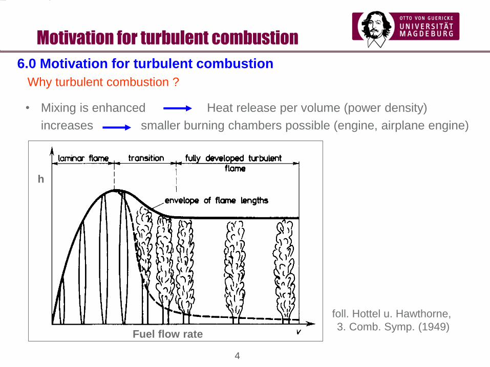
6.0 Motivation for turbulent combustion

Why turbulent combustion ?

• Mixing is enhanced Heat release per volume (power density)

increases smaller burning chambers possible (engine, airplane engine)

foll. Hottel u. Hawthorne,

3. Comb. Symp. (1949)Fuel flow rate

h

5



Why turbulent combustion ?

Pratt & Whitney

PW4000 Engine

e.g. Boeing 747-400

Airbus A310-300

6


• time dependent fluctuating velocities

• three dimensional

• eddy structures (e.g. Karman's eddy street)

2 possible approaches:

• statistical

• -> Mean value

• -> Standard deviation etc.

• structural

• eddy description, LES, DNS

Turbulence quantities

6.2 Turbulence Quantities

Turbulent Flow:

an einem Ort x gemessen

t

u(t)

)()( tuutu

7



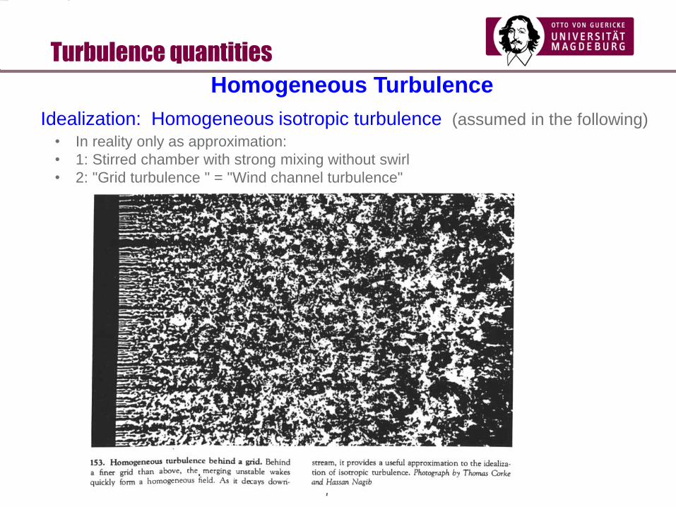
Idealization: Homogeneous isotropic turbulence (assumed in the following)

• In reality only as approximation:

• 1: Stirred chamber with strong mixing without swirl

• 2: "Grid turbulence " = "Wind channel turbulence"

Homogeneous Turbulence

8


Homogeneous Turbulence


Common statistical approach: Reynolds decomposition

"Turbulence degree" (v. Kármán Number)

(typ. Tu < 10% for grid turbulence )

(6.1)

2)(

)()(

tuuu

tuutu

rms

Mean value

"Turbulence intensity" (Fluctuation velocity =

Root-Mean-Square Velocity)

0)( tu

(6.2)

(6.3)

u

uTu

(6.4)

an einem Ort x gemessen

t

u(t)

)()( tuutu

9



Concept of Eddy cascade

Eddies of different size

"Concept of eddy cascade" (eddy spectrum)

Hindrance -> Large eddies -> smaller eddies -> very small eddies

-> Molecular dissipation

(to heat)

"Integral length scale" Lx "Kolmogorov-scale" h (or lk )

("Macro length scale") ("Micro length scale")

(Energy transport = Dissipation rate e)

10



Transition laminar - turbulent

Reynolds number

"Turbulent Reynolds number"

Note: Ret is about 100 - 1000 times smaller than Re

DuRe

Note: depends on geometry !

D = geometrical size

= kin. viscosity

Rekr 2200 Flow in tube

100 - 1000 Axial free jet flow

(6.5)

x

t

LuRe

Independent from geometry !

characteristic local quantity

turbulent: Ret > 1

(6.6)

11



Turbulence characterization:

(Assumption: fully developed turbulence, homogeneous, isotropic)

Turbulent fluctuation velocity u' = urms (measured)

Integral length scale (Macro length) Lx (measured)

Turbulent Reynolds number Ret = u' Lx / (6.7)

Kolmogorov length (Micro length) h = Lx / Ret3/4 (6.8)

Increase of turbulent Reynolds number broadens turbulence spectrum

Note aside: in some articles the Taylor length is used:

Taylor length ll = 6,3 Lx / Ret1/2 (6.9)

Local mean turbulent strain rate a = u' / ll (6.10)

(Scherrate)

12


Turbulent premixed flames

6.2 Turbulent premixed Flames


• Fuel and air are premixed

• Danger of flash back

• Lean premixed flames can have low pollutant emissions:

• No soot

• Very low NOX formation (stationary gas turbines, 'Blue burner')

• Turbulence increases the density of reaction (Pthermal / Vflame). How ?

6.2.1 Structure of turbulent premixed flames

6.2.2 The Borghi diagram

6.2.3 Turbulent flame speed

6.2.4 Flamelet model for calculation of turbulent premixed flames

13




Bunsen

flame

(Heidelberg)

D=80 mm

100 kW

Photograph:

Laser-

diagnostics

(15x10 cm)

14




Flame brush

(Flammen-

zone)

Flame front

(Flammenfront)

Several instantaneous images Average image

Fuel + Air

15



Turbulence - Flame Interaction

Turbulent flow field has strong influence on

premixed flames

• Details of turbulence-flame interaction only barely known for long time.

• Theoretical analysis:

Regime diagram following Borghi and Peters

• Experimental verification was difficult for long time

• Flame front fluctuates fast

• Spatial flame structure < 1mm

16



Borghi diagram (Borghi 1985, Peters 1986)

laminar

Ret = 1

Turbulence

intensity

(normalized

)

Turbulence

macro

length

(normalized)

L

xL

log

Ls

ulog Ret =

100

Ret = 104 Ret = 106

Two Turbulence

quantities: u', Lx

Scaled with two laminar

flame quantities sL, L

Log. Scales

Ret = u' Lx /

indicates transition:

laminar - turbulent

and intensity of turbulence

Assumption: Le = a/D = 1

and Sc = /D = 1

hence:

turbulent

Zeld

LLsa

17


Da <<1

Da >>1

Damköhler (Turn over time of large eddy)

number (Transit time through lam. flame)

Turbulent Regime:

Two extreme Cases:

mixing time << reaction time

reaction time << mixing time

"Stirred reactor"

"Wrinkled laminar flame"

(however in a turbulent flow)


Time Scales

LL

x

reak

turb

s

uLDa

/

/

laminar

Ret = 1

Turbulence

intensity

(normalized

)

Turbulence -

Macro

length

(normalized)

L

xL

log

Ls

ulog

turbulent"Stirred reactor"

fast mixing

Da << 1

Da = 1

Da >> 1 fast chemistry

(6.11)

L

"Wrinkled laminar flame"

18



Length Scales

Model:

Large Eddies ( l >> L) -> wrinkle flame front

Small Eddies ( l << L) -> enter the flame front, increase diffusive transport

within the flame front ->

they thicken the flame front

L

Reaction zone

Lx

unburnt burnt

hComparison of length scales:

Karlovitz number:

Ka = (L / h )²

with smallest "Kolmogorov-Eddies"

h = Lx / Ret3/4

(6.12)

19



Distributed reaction zone

Model for the regime of distributed

reaction zones

(foll. Turns)

Above which limit the smallest

eddies enter the reaction zone ?

Supposition

("Klimov-Williams Criterion"):

Thickening, if h < L

i.e. Ka > 1 (6.13)

20



Borghi diagram

laminar

"stirred reactor"

Da = 1

Ka = 1

L

Turbulenc

eintensity

(norm.)

Turbulence-

macro length

(norm.)L

xL

log

Ls

ulog

u' = sL

Ret =

1

"thickened

flames"

"Wrinkled flames"

"Corrugated

flames"

"verdickte turbulente

Flammen"

"Gewellte

Flammen"

"Gefaltete

Flammen"

fast mixing

Da << 1

Da >> 1 fast chemistry

21



Turbulent flame speed sT

Definition: 'turbulent flame speed' sT

Idea: Kinematic Balance between

turbulent flame speed sT and the

normal velocity component un for

stationary flames.a

sT un

u

sTasin

u

u

22




Height of flame

as approximation

with unburnt gas velocity u and angle

a between u and flame front.

For Bunsen flame (assumed u =

const.) follows with

as (rough) approximation the flame

height H.

u

sTasin

a

sT un

H

R

u

sTasin

H

Ratan

(6.14)

(6.15)

u

u

23




Turbulent flame speed sT is effective propagation velocity of premixed flame

in turbulent flow field.

Necessary for calculation:

• Relation for sT as function of

• flame parameters (fuel, stoichiometry, p, T --> sL)

• Turbulence parameters (u', Lx , Ret , Da, ...)

Is discussed in literature with several different approaches:

• Theory (Damköhler 1940): For wrinkled laminar flame surfaces the turbulent

reaction rate and thus also the turbulent flame speed is proportional to

geometrical flame surface area

LT

L

L

T

s

u

A

A

s

s ' 1 (6.16)

24




Measurements of flame propagation in turbulent stirred ignition bomb experiments

(Bradley et al.): Correlation from Gülder (1990)

Measurement of normal component un directly before the flame front as function of

turbulence and flame parameter from Liu et al. (1993)

Zimont (1995) (for u' > sL), A = 0,5 ... 1

25,0

5,0

' 62,01 t

LL

T Res

u

s

s

44,0

4,0

' 435,01 t

LL

T Res

u

s

s

Ret = 150

0

5

10

15

20

25

0 5 10 15 20

u'/sL

sT/s

LDamköhler

Gülder

Liu ...

(6.17)

(6.19)

2/1

4/14/1 '

L

t

L

T

s

uRePrA

s

s

(6.18)

25



Calculation of turbulent premixed flames

• Numerical calculation procedure for turbulent premixed flames is difficult

• Aim: Combustion model to be coupled to computational fluid dynamics

(CFD)

• Not yet for practical applications, current research topic

• Possible approach:

Borghi diagram shows:

Typical: Wrinkled thin flame fronts, locally similar to laminar, if Ka < 1

(Measurement (--> LTT) shows, even if Ka < 10 ... 100)

then ...

26



“Flamelet“ –Approach: Peters 1986

For laminar-like wrinkled flame fronts a decoupling is possible between

turbulence and reaction :

• Turbulent flow field wrinkles the flame

• Reaction remains similar as in laminar case (maybe modified from

curvature or strain effects)

Flamelet-approach simplifies numerical calculation significantly !

Calculate basically the place of reaction (averaged), while the detailed

chemistry is known from laminar flames.

27



“Flamelet“ –Approach

for that introduce a mean reaction progress variable

For this variable basically one balance equation is enough instead of N

equations for energy and species.

This equation can be calculated numerically together with the flow field

(+ turbulence model).

Several approaches for this c-equation (sometimes also called G- or S-

equation) are discussed in the literature

One approach, based on turbulent flame speed, gives e.g.

(Dinkelacker, Helbig, Hölzler 1999): (next page)

c

0

0

TT

TT c c

max

:remember gas burnt find toy Probabilit

28

Idea:

• Average reaction rate ~Turbulent flame speed

• This yields a "Turbulent-Flame-Speed-Closure" for averaged reaction term

(Zimont & Lipatnikov 1995)

• Turbulent burning velocity, e.g., from equation (6.19), for application with

pre-factor of A = 0,52 (Zimont & Lipatnikov 1995)

• Solution as subroutine with standard-CFD-program (e.g.,Fluent)

place of reaction

cxsw Tuc ˆ

Example for Flamelet-Model Turbulent-Flame-Speed-Closure (TFC)

(6.21)


29



Testcase: turbulent premixed V-flame: Reaction progress c

Simulation

Experiment

2-dim. Rayleigh-

Thermometry (A.

Soika)

l = 1.43 l = 1.72 l = 2.00

1,0

0,9

0,8

0,7

0,6

0,5

0,4

0,3

0,2

0,1

0,0

c

30


D = 80 mm

1,0

0,9

0,8

0,7

0,6

0,5

0,4

0,3

0,2

0,1

0,0

Reaction Progress

140

120

1,0

0,9

0,8

0,7

0,6

0,5

0,4

0,3

0,2

0,1

0,0

Reaction Progress

Experiment

(Heidelberg) Numerics

Testcase: 80 mm - Bunsen Flame

(F. Dinkelacker, R. Muppala, SIAM 2002)

c c


31


Turbulent non-premixed flames

6.3 Turbulent non-premixed flames

• Fuel and air are mixed in burning chamber

• Turbulence supports mixing

• Large practical relevance

• Also for solid and liquid fuels

• Disadvantage: More pollutants and soot as premixed flames

3.1 Examples

3.2 Flame length

3.3 Mixture fraction-concept

32



Snap-shot of a turbulent jet-

diffusion flame (schematics)

33



Example: Burning chamber of air gas turbine (schematic)

Use of non-premixed (diffusion) flames owing to safety reasons (flashback)

34



Mixture fraction concept

Numerical calculation of diffusion flame

Aim: Numerical calculation of flame location and flame length.

Models for diffusion flames often are based on observation, that mixing

controls the reaction. Then the flow field couples with mixture fraction f ;

to be calculated instead of species and temperature:

Allocation only once (ideal situation, see -> )

) ,( fieldfraction Mixture

) ( field Turbulence

) ( averaged field, Flow

ff

k,

p,ui

e

ondistributi Species

releaseHeat

field eTemperatur ,

ff

ffst10

YBrYPr

T

YOx

Mixture fraction approach (like lam. Fla.)

35




Temperature as function of mixture fraction

Turbulent non-premixed hydrogen jet flame, left: low turbulence, right: higher

turbulence intensity

Measured (Laser-Raman-Scattering) vs. equilibrium calculation

(Magre, Dibble 1988, cit. after Warnatz et. al. 96)

36




Example: Mixing field of a typical non-premixed turbulent flame

Mixture fraction, instantaneous

distribution (iso-line for f = 0,07)

Mixture fraction, mean value

Mixture fraction, average

fluctuations

f. Bilger

37


Summary

Turbulent combustion to enhance mixing

• Turbulence-Flame Interaction

• Two extreme cases allow 'separation' of turbulence and reaction:

• 'Fast mixing limit' (Stirred reactor model):

spatially homogeneous chem. reactions

• 'Fast chemistry limit': Wrinkled laminar 'flamelet'

'flamelet' - approach


• Typically: fluctuating wrinkled thin flame fronts result in a broad

flame brush

• Turbulent flame speed sT

• Flamelet models for calculation

Turbulent diffusion flames

• Turbulence enhances fuel-air mixing

• Mixture fraction concept

38



Results of experiment of premixed turbulent flame structure

No significant

thickening

(partly even thinned

flames instead *)

Thin reactions zone,

Locally modified

preheat zone

V 8 hkalt

0,1

1

10

100

0,1 1 10 100 1000

l x / L

u'/s L

h0 = F

hi = i

Ret = 600

* Dinkelacker, 20. Deutscher Flammentag, VDI-Berichte Nr. 1629, S. 473 (2001)

Range of wrinkled laminar-like flames (Flamelet) is more extended

Details, see *

39




foll. Bradley,

24. Comb. Symp. (92):

RL = turb. Reynolds number

Le = Lewis number

K = dimensionless

Strain rate

sT

/ s

L

u' / sL

LLLL s

u

s

aK

l

'

Critics:

Measured flames

have been very small

40




For increasing turbulence (u'/sL) the turbulent flame speed increases slower

("Bending Effect").

Possible reasons:

• Flame area increases not with u'/sL, but annihilates due to interaction

• Reaction locally reduced compared with "laminar flamelets", due to

• local curvature

• Influence of small scale eddies

• local breaks in reaction front (flame quench) ?

For further increase of u'/sL flame quenches totally.

41



Length of turbulent jet non-premixed flames

Length of flame nearly independent on fuel exit velocity, for developed

turbulent flame

Fuel flow rate

42



Length of turbulent jet non-premixed flames

Empirical relation for flame length of turbulent jet non-premixed flame

(Delichatsios 93, Turns 96)

Length of diffusion flame is controlled by mixing. From that the following relation is

derived for jet flames (here for "sufficiently" large momentum of the fuel flow,

buoyancy is neglected, calm surroundings; for other conditions see Turns 96).

stB

L

Bj

fY

d

L,

/ 21

23

Flame length Lf

Diameter of fuel inlet dj

Density ratio between fuel and air B/L

Stoichiometric fuel mass fraction YB,st (Lecture 2,

Table 2.1)

Note:

Length of flame is (approx.) independent of inlet velocity !

Length of flame is proportional to diameter of inlet!

Length of flame depends on fuel

Example: Methane in air, dj = 10 mm, gives length Lf = 3,1 m

(6.20)

43



Example: rotary furnace

Turbulent diffusion flame in rotary furnace for production of cement

(n. Görner)

44


0

1

2

3

0 1 2 3

Ret

Lx

h

(Assumption: fully developed turbulence, homogeneous, isotropic)

Turbulent fluctuation velocity u' = urms (measured)

Integral length scale (Macro length) Lx (measured)

Turbulent Reynolds number Ret = u' Lx / (6.7)

Kolmogorov length (Micro length) h = Lx / Ret3/4 (6.8)

Increase of turbulent Reynolds number broadens turbulence spectrum

content of lecture - otto von guericke university · pdf filecontent of lecture 1....

Documents