REPORT No.2/11_20_2001

1

CONTAINER MOVEMENT BY TRUCKS IN METROPOLITAN NETWORKS: MODELING AND OPTIMIZATION1

Hossein Jula∗, Maged Dessouky∗∗, Petros Ioannou∗♣, and Anastasios Chassiakos∗∗∗

* Department of Electrical Engineering, University of Southern California, Los Angeles, CA 90089-2562

** Department of Industrial and Systems Engineering, University of Southern California, Los Angeles, CA 90089-0193

*** College of Engineering, California State University at Long Beach, Long Beach, CA 90840-5602

♣ Corresponding author: Email: ioannou@rcf.usc.edu, Tel: (213) 740 4452

Abstract:. Today, in the trucking industry, dispatchers still perform the tasks of cargo assignment, and driver scheduling. The growing number of containers processed at marine centers and the increasing traffic congestion in metropolitan areas adjacent to marine ports, necessitates the investigation of more efficient and reliable ways to handle the increasing cargo traffic. In this paper, it is shown that the problem of container movement by trucks can be modeled as an asymmetric “multi-Traveling Salesmen Problems with Time Windows” (m-TSPTW). A two-phase exact algorithm based on dynamic programming (DP) is proposed that finds the best routes for a fleet of trucks. Since the m-TSPTW problem is NP-hard, the computational time for optimally solving large size problems becomes prohibitive. For the case of medium to large size problems, we develop a hybrid methodology consisting of DP in conjunction with genetic algorithms. Computational results demonstrate the efficiency of the exact and the hybrid algorithms.

Keywords: Modelling systems, Travelling salesman, Dynamic programming, Genetic Algorithms, Routing.

1 This work is supported by METRANS located at University of Southern California and The California State

University at Long Beach, and by the National Science Foundation under grant DMI-9732878. The contents of this paper reflect the views of the authors who are responsible for the facts and the accuracy of the data presented herein.

REPORT No.2/11_20_2001

2

I. INTRODUCTION

The growth in the number of containers has already introduced congestion and

threatened the accessibility to many terminals at port facilities [24]. The congestion at a

port, in turn, magnifies the congestion in the adjacent metropolitan traffic network and

affects the trucking industry on three major service dimensions: travel time, reliability,

and cost. Trucking is a commercial activity, and trucking operations are driven by the

need to satisfy customer demands and the need to operate at the lowest possible cost

[18].

Today, in the trucking industry, human operators (dispatchers) still play the major

role in cargo assignment, route planning and driver scheduling. Dispatchers inform

drivers about traffic conditions, in addition to assisting them in departure/arrival

decisions and providing navigational information [19]. Dispatchers currently obtain

information about traffic conditions, mostly through radio traffic reports and through

information relayed back by the drivers [11]. The growing number of containers at

marine centers and the increasing traffic congestion in metropolitan areas necessitates

the investigation of more efficient, reliable and systematic ways to handle the increasing

amount of cargo in a metropolitan traffic network.

The purpose of this paper is to investigate methods for improving the scheduling of

trucks, where ISO containers2 need to be transferred between marine terminals,

intermodal facilities, and end customers. The objective is to reduce empty miles, and to

improve customer service. As a consequence of reduced miles and better service,

container terminals can become more competitive, vehicle emissions will be reduced,

and drivers will incur less congestion related delays.

2 Most containers are sized according to International Standards Organization (ISO). Based on ISO, containers are

described in terms of TEU (Twenty-foot Equivalent Units) in order to facilitate comparison of one container system with another. A TEU is 8 feet wide, 8 feet high and 20 feet long container. An FEU is an eight-foot high forty-foot container and is equivalent to two TEUs.

REPORT No.2/11_20_2001

3

In this paper, we show that the container movements by trucks in metropolitan areas

can be modeled as a multi-Traveling Salesmen Problem with Time Windows (m-

TSPTW). This problem is often referred to as the full-truck-load problem in the

academic literature [22]. The problem entails the determination of routes for the fleet of

trucks so that the total distribution costs are minimized while various requirements

(constraints) are met. The m-TSPTW is an interesting special case of the Vehicle Routing

Problem with Time Windows (VRPTW) where the capacity constraints are relaxed.

Savelsbergh [21] has shown that finding a feasible solution to the single Traveling

Salesman Problem with Time Windows (TSPTW) is an NP-complete problem.

Although there has been a significant amount of research on the VRPTW (e.g., see

[2, 4, 5, 7, 10, 14]), there has been little work on the m-TSPTW. Since the m-TSPTW is

a relaxation of the VRPTW, it may appear at first that the procedures developed for the

latter could be applied to the m-TSPTW. However, as Dumas et al. [6] point out, these

procedures are not well suited to the m-TSPTW. Hence, new procedures need to be

developed for the m-TSPTW. We note that Dumas et al. [6] presented an efficient exact

solution procedure for the single vehicle TSPTW. However, in contrast to the simple

transformation of the m-TSP to the TSP, m-TSPTW cannot be easily converted to a

single vehicle TSPTW.

The main contributions of this paper are as follows: 1) we show that the container

movements by trucks can be modeled as a m-TSPTW problem, and 2) we propose the

following two methodologies for solving the m-TSPTW problem.

a. An exact method based on Dynamic Programming (DP) is proposed. The

method consists of two phases: 1) generating feasible solutions, and 2) finding

the optimum solution among all feasible solutions (set-covering problem).

Computational experiments show that the proposed exact method can optimally

solve problems with up to 15-20 nodes on randomly generated problems.

REPORT No.2/11_20_2001

4

b. For medium size problems, we develop a hybrid methodology consisting of

dynamic programming for generating feasible solutions in conjunction with

genetic algorithms (GA). The GA algorithm is used to find a ‘good’ solution

among all feasible solutions. Experimental results show the efficiency of the GA

set-covering algorithm for medium to large size problems.

The paper is organized as follows. In Section II, the container movement and

trucking operations in metropolitan areas are described. The problem is formulated as an

asymmetric m-TSPTW. In Section III, the existing solution methods for the TSPTW

and m-TSPTW are briefly reviewed, and two methodologies for solving the m-TSPTW

problem are proposed. Section IV concludes this paper.

II. CONTAINER MOVEMENT: PROBLEM DESCRIPTION AND FORMULATION

In this section, it is shown that the container movements by trucks can be modeled as

an asymmetric multi-Traveling Salesmen Problem with Time Windows (m-TSPTW). We

start with describing the container movement and trucking operations in metropolitan

areas.

II.1. Problem Description

Today, in the trucking industry, human operators (dispatchers) perform the tasks of

cargo assigning, route planning and driver scheduling. Each day, the list of containers to

be handled during the day is passed to the dispatcher early in the morning. The list

contains information about the origin and the destination of containers. The dispatcher

assigns a driver to each container based on the availability of the driver and his/her skills.

In today’s container industry, there is a lot of discussion about appointment windows.

The appointment systems are being considered as part of a solution for terminal

congestion. These systems are becoming more important because of the terminals’ need

to 'manage the demand' (the flow of trucks). For instance, the Hanjin terminal at the

REPORT No.2/11_20_2001

5

Port of Long Beach has just started informing the local trucking companies of the list of

containers they want to be picked up on the hoot shift (i.e., 3:00 a.m. - 7:00 a.m.).

The problem of interest can be stated more formally as follows: A set of loads

(containers) needs to be moved in a metropolitan (local) area. The local area contains

one truck depot (which thereafter will be called depot), as well as many end customers

including marine terminals and intermodal facilities. Associated to each load is hard time

windows imposed by customers for pickup and delivery at origin and destination points,

respectively.

A set of trucks (vehicles) is deployed to move the loads among the customers, and

the depot. Each truck can only serve a single load (e.g. one FEU3 size container) at a

time, and initially, all trucks are located at the depot. We assume that each driver may not

be at the wheel for more than a certain number of hours (working shift) in each working

day and has to drive his truck back to the depot within this time limit.

The objective is to minimize the total cost of providing service to the loads within

their specified time constraints.

Let L be a set of n cargos (containers) to be transferred in a transportation network

G, i.e., L={l1,l2,…,ln}; and V be a set of p vehicles labeled vm, m=1,2,..,p assigned to

transfer the containers, i.e., V={v1,v2,…,vp}.

We assume that, at any time, a vehicle vm∈V can transfer at most a single container,

say li∈L, and that the information of the origin and the destination of container li is

known in advance. We denote by O(li) and D(li) the origin and the destination of

container li, respectively. Container li must be picked up from its corresponding origin

during a specific period of time known as the pickup time window and denoted by

3 FEU: Forty-foot Equivalent Units (See also footnote 2).

REPORT No.2/11_20_2001

6

],[ )()( ii lOlO ba . Likewise, container li must be delivered at its corresponding destination

during a delivery time window denoted by ],[ )()( ii lDlD ba .

Let K(m) be the total number of containers assigned to be transferred by vehicle

vm∈V. Let also δmk∈L be the kth container assigned to vehicle vm. The sequence of

containers assigned to vehicle vm is called a route and is denoted by rm, i.e. rm={δm1,

δm2,…,δmk,…,δmK(m)}. Route rm is said to be feasible if it satisfies the time window

constraints at the origins and the destinations of all assigned containers, and the total

time needed for traveling on the route is less than a certain amount of time called the

working shift (time) and denoted by T.

Figure 1 shows three routes (r1, r2, and r3) starting from the depot and ending at the

same depot. Solid lines, in Figure 1, illustrate the traveling between the origin and the

destination when the vehicle is loaded, while dashed lines indicate empty traveling

between the destination of the last drop-off and the origin of the next pick-up.

Let's denote by f(rm) the cost associated with each route m.

∑∑==

++=

)(

0)()(

)(

1)()( 1

)(mK

kOD

mK

kDOm mkmkmkmk

ccrf δδδδ ( 1 )

Where:

− )()( mkmk DOc δδ is the cost of carrying the kth container from its origin to its

destination, and

− )()( 1+mkmk ODc δδ is the cost of empty travel between the destination of the kth

container to the origin of the (k+1)th container. The depot is denoted by k=0

and k=n+1.

REPORT No.2/11_20_2001

7

Figure 1: Typical routes starting from depot and ending at the same depot. The large empty circle denotes the depot. Each small black circle denotes the origin (O) or the destination (D) of a container.

The objective is to find optimum routes for the p vehicles providing the services to

the n containers by traveling between origins and destinations of containers and

satisfying the time window constraints such that the completion of handling all

containers results in minimizing the total travel cost. The objective function, J, can be

written as follows:

∑=

=p

mmrfMinJ

1)( ( 2 )

Let's assume that the travel cost for a vehicle, either loaded or empty, is static and

deterministic, and the cost associated with transferring a container li∈L between its

origin and destination, )()( ii lDlOc , is independent of the order of transferring the

Route r1

Route r2

Route r3

O(δ31)

D(δ31)

O(δ32)

D(δ32)

O(δ33)

D(δ33)

O(δ11)

O(δ12)

O(δ13)

D(δ13)

D(δ12) D(δ11)

D(δ21)

O(δ21)

Route r1

Route r2

Route r3

O(δ31)

D(δ31)

O(δ32)

D(δ32)

O(δ33)

D(δ33)

O(δ11)

O(δ12)

O(δ13)

D(δ13)

D(δ12) D(δ11)

D(δ21)

O(δ21)

REPORT No.2/11_20_2001

8

container by a vehicle. Let’s also assume that the fleet of vehicles is homogenous.

Therefore, no matter what the assignment and order of handling the n containers are,

the costs (.)(.)DOc don't affect the cost function in ( 2 ) and can be considered to be

fixed. That is, the total cost function in ( 2 ) is only affected by the cost associated with

vehicles' empty traveling between the destinations of the kth and (k+1)th containers; and

the problem of interest is reduced to finding the best feasible assignment and sequencing

of n containers to p vehicles such that the total empty travel cost of the vehicles is

minimum.

Figure 2: Each origin-destination pair in Figure 1 can be grouped as a node.

Thus, each origin-destination pair, O(δmk)-D(δmk), in Figure 1 can be replaced by a

node OD(δmk) where δmk∈ rm and k=1,...,K(m), and the cost between two nodes is equal

to the cost of empty travel between the destination of the first node to the origin of the

second one (see Figure 2).

OD(δ11)OD(δ12)

OD(δ13)

Route r1

Route r2

Route r3

OD(δ21)

OD(δ31)

OD(δ32)OD(δ33)

OD(δ11)OD(δ12)

OD(δ13)

Route r1

Route r2

Route r3

OD(δ21)

OD(δ31)

OD(δ32)OD(δ33)

REPORT No.2/11_20_2001

9

The time window at node OD(δmk) can be expressed in terms of: 1) time window at

its origin, 2) time window at its destination, and 3) the traveling time between the origin

and the destination, )()( mkmk DOt δδ . Figure 3 demonstrates a typical relation between these

three factors and the time window ],[ DD ba ′′ , where ],[ DD ba ′′ is the time window at the

destination shifted back in time by )()( mkmk DOt δδ . For the sake of simplicity, we eliminate

all subscripts δmk in Figure 3.

Figure 3: Time window at origin [aO, bO], destination [aD, bD], and time window at destination shifted back in time [a’D, b’D].

Figure 4 presents all possible situations between time windows ],[ DD ba ′′ and

],[ OO ba . The dashed areas, in Figure 4, indicate the time window at the origin of node

OD during which a vehicle can be loaded and yet meet the time window constraint at the

destination. Case IV is infeasible and cannot happen in a real situation.

The problem of interest can now be restated as follows: p vehicles are initially located

at the depot. They have to visit nodes OD(li), i=1,..,n. The task is to select some (or all)

of these vehicles and assign routes to them such that each node is visited exactly once

during the time window ],[ii ll ba , where ],[

ii ll ba is expressed as follows (see Figure 4).

),( min )()()()(

)(

iiiii

ii

lDlOlDlOl

lOl

tbbb

aa

−=

= ( 3 )

aOaD

a’D

bObD

tOD

b’D

aOaD

a’D

bObD

tOD

b’D

time

REPORT No.2/11_20_2001

10

Figure 4: All possible situations between time window at origin, and time window at destination shifted back in time. The dashed area presents the time window at node OD.

The problem now falls in the class of asymmetric Multi-Traveling Salesmen Problems

with Time windows (m-TSPTW). In m-TSPTW, m salesmen are located in a city (i.e.

node: n+1) and have to visit n cities (nodes: 1,..,n). The task is to select some or all of

the salesmen and assign tours to them such that in the collection of all tours together the

cost (distance) is minimized and each city is visited exactly once within a specified time

window [20]. The problem is asymmetric since the traveling cost between each two

nodes i and j depends on the direction of the move. Note that,

.)()()()()()()()( ijijjiji lODlODlOlDlOlDlODlOD cccc =≠= ( 4 )

II.2. M-TSPTW Mathematical Formulation

Let G=(ND,A) be a graph with node set ND={o,d,N} and arc set A={(i,j)| i, j ∈

ND}. The nodes {o} and {d} represent the single depot (origin-depot and destination-

depot), and N={1,2,…,n} is the set of customers. To each arc (i,j)∈A, a cost cij and a

����������������������������������������������������������������aO

a’D

bO

b’D

������������������������aO

a’D

bO

b’D

����������������������������������������������������������������aO

a’D

bO

b’D

aO

a’D

bO

b’D

��������������������������������������������������������������������������������aO

a’D

bO

b’D

������������������������������������aO

a’D

bO

b’D

I II III

IV V VI

����������������������������������������������������������������aO

a’D

bO

b’D

������������������������aO

a’D

bO

b’D

����������������������������������������������������������������aO

a’D

bO

b’D

aO

a’D

bO

b’D

��������������������������������������������������������������������������������aO

a’D

bO

b’D

������������������������������������aO

a’D

bO

b’D

I II III

IV V VI

REPORT No.2/11_20_2001

11

duration of time tij are associated representing the cost and the time of traveling between

nodes i and j, respectively. In addition, to each node i∈ ND, a service time si and a time

window ],[ ii ba are associated. The service time si is the duration of time for a vehicle to

be served at node i, and ai and bi are the earliest and latest time to visit node i,

respectively. An arc (i,j)∈A is feasible iff jijii btsa ≤++ . Let V be the set of vehicles

v. A route in the graph G is defined as assigning a set of nodes rv={o, wv1,wv

2,…,wvk, d}

to vehicle v such that each arc in rv belongs to A, and the time that service begins at node

j∈ rv is within the time window of that node. Let's also define:

xvij=1 if arc (i,j)∈A is traveled by vehicle v and is in the optimal path4. xv

ij=0

otherwise,

Tvi is the time when service begins at node i by vehicle v.

The m-TSPTW can be formulated as follows:

4 The optimal path is a cycle of all nodes with the smallest possible total cost of arcs.

REPORT No.2/11_20_2001

12

Constraints ( 5b ) require that only one vehicle visit each node in N. Constraints ( 5c )

ensure that at most |V| number of vehicles are used. To fix the number of vehicles, the

inequality should be replaced by equality. Constraints ( 5d ) guarantee that the number of

vehicles leaving node j is the same as the number of vehicles entering the node.

Therefore, constraints ( 5b )-( 5d ) together enforce that at most |V| number of vehicles

visit all nodes in N only once. Constraints ( 5e ) enforce the time feasibility condition on

consecutive nodes. Constraints ( 5f ) specify the time window constraints at each node.

Constraints ( 5g ) require that each vehicle shall be used less than a certain number of

hours per day, and finally constraints ( 5h ) are the binary constraints.

III. PROPOSED SOLUTION METHODS FOR M-TSPTW

The m-TSPTW is an interesting special case of the Vehicle Routing Problem with

Time Windows (VRPTW) where the capacity constraints are relaxed. Consequently, one

may think of applying the same solution methods for m-TSPTW by relaxing the capacity

Min ∑ ∑∈ ∈Vv Aji

vijij xc

),( ( 5a )

Subject to

∑ ∑∈ ∪∈

=Vv dNj

vijx}{

1 ∀ i∈N ( 5b )

∑∑∈ ∈

≤Vv Nj

voj Vx ∀ i∈N, v∈V ( 5c )

∑ ∑∪∈ ∪∈

=−}{ }{

0dNj oNj

vji

vij xx ∀ i,j∈ND,

v∈V ( 5d )

0)( ≤−++ vjiji

vi

vij TtsTx ∀ i,j∈ND,

v∈V ( 5e )

iv

ii bTa ≤≤ ∀ i∈ND, v∈V ( 5f )

TTT vo

vd ≤− ∀ v∈V ( 5g )

{ }1 ,0∈vijx ∀ (i,j)∈A,

v∈V ( 5h )

REPORT No.2/11_20_2001

13

constraints in the VRPTW. Although the idea of using solution methods on VRPTW in

m-TSPTW looks very rational, the experimental results show otherwise. In their work,

Dumas et al. [6] state: ‘Even though the TSPTW is a special case of VRPTW, the best known

approach to the latter problem [4] is not well suited to solve the TSPTW. This column generation

approach would experience extreme degeneracy difficulties in this case.’

In the shed of this light researchers have sought methods tailored for the TSPTW

and m-TSPTW. However, despite the importance of m-TSPTW in the trucking

industry, research on m-TSPTW has been scant [5].

III.1. Solution Methods for TSPTW and m-TSPTW

Since finding a feasible solution to the TSPTW and m-TSPTW is a NP-complete

problem [21], most research has focused on heuristic algorithms. Lin and Kernighan [16]

proposed a heuristic algorithm based on a k-interchange concept for the TSPTW. The

method involves the replacement of k arcs currently in the solution with k other arcs.

Lee [15] developed two heuristics based on the Vehicle Scheduling Problem (VSP) for

the m-TSPTW. The VSP algorithms are exact in that they can find the optimal solution

to the VSP in polynomial time. However, solutions found by VSP algorithms may be

infeasible for the m-TSPTW. Two construction heuristics are developed to assign each

customer to a route. Improvement heuristics are then developed to combine the initial

routes. Calvo [3] proposed the use of a new heuristic method for the TSPTW based on

solving an auxiliary assignment problem. To find better solutions, the algorithm uses two

objective functions. When the algorithm gets trapped in a local minimum, it uses the

second objective function to widen its neighborhood region. Gendreau et al. [9]

developed a generalized insertion heuristic algorithm for TSPTW. The algorithm

gradually builds a route by inserting at each step a vertex on to the route, and performing

a local optimization. Once a feasible route has been determined, a post optimization

algorithm is used to improve the objective function.

REPORT No.2/11_20_2001

14

Despite the difficulty of the TSPTW, few authors have focused on exact solution

approaches. Dumas et al. [6] used Dynamic Programming (DP) enhanced by a variety of

elimination tests to solve the single vehicle TSPTW optimally. These tests took

advantage of the time window constraints to significantly reduce the number of arcs in

the graph to eliminate states. The authors managed to solve problems of up to 200

nodes with small window size, and problems of up to 80 nodes with larger time

windows.

As we noted previously, in contrast to the relation between the TSP and the m-TSP

(see [20]), the m-TSPTW cannot be transformed into an equivalent TSPTW. In this

paper, the following methodologies are developed to extend the earlier work on the

single vehicle TSPTW:

− An exact two-phase Dynamic Programming (DP), and

− A hybrid methodology consisting of DP in conjunction with genetic algorithms

(GA),

We next describe our approaches for solving the m-TSPTW.

III.2. Proposed Exact Method for m-TSPTW

A two-phase Dynamic Programming (DP) based method is proposed for solving m-

TSPTW. The method is an extension of the algorithm used for the TSPTW and

proposed in [6]. However, contrary to [6], partial paths, which cannot be extended to

other nodes, will not be eliminated, as it may be on the optimum set of solutions.

Moreover, at each node tests are conducted to ensure the reachability of the depot

according to constraint ( 5g ).

In phase one, of the exact method, a forward DP is used to generate all feasible

solutions, which will be called states. To reduce the computational time and the number

of states, extensive elimination tests are performed before and during running the DP

REPORT No.2/11_20_2001

15

algorithm. The elimination tests take advantage of the time window constraints in ( 5e ),

( 5f ) and ( 5g ) to significantly reduce the number of states. The outcome of the first

phase will be sets of feasible solutions. The sets, then, will be fed to another DP

algorithm in order to find a set of routes with minimum total cost which covers all

nodes. That is, the second DP solves a set-covering problem in order to extract the

optimum set of solutions among all sets of solutions. In the followings, we explain the

exact method in detail.

III.2.1. Methodology:

Phase One: We require that the triangular inequality hold for both the travel costs

and the travel times between each two nodes of the graph G (see Section II for

definition of G). That is, for any i,j,k∈ND, we have cik ≤cij +cjk and tik ≤tij +tjk. Let i∈S

be the last visited node by vehicle v (i.e., on path v); t be the time at which service begins

at node i; and S⊆N be an unordered set of visited nodes. Associated to each state (S,i,t),

defined above, is a cost denoted by F(S,i,t) and defined as the least cost with minimum

spanned time of a path starting at node {o}∈ND passing through every node of S

exactly once and ending at node i. Note that, there are several paths that visit set S and

end at node i. Among them, we choose the one with minimum cost and minimum

spanned time (see the state elimination test 2, below). Let also fr(S)∈N be the first node

in set S. The starting time of set S is denoted by tfr(S)and is defined as tfr(S)= max(ao, afr(s)

– so – to,fr(s)). This time indicates the earliest possible vehicle dispatching time from the

depot such that no waiting time is necessary at node fr(S).

In order to reduce the computational time, two types of elimination tests are

performed: arc elimination, and state elimination.

1) Arc elimination tests: The arc elimination tests take advantage of the time window

constraints ( 5e ), ( 5f ) and ( 5g ) to significantly reduce the number of states. These tests

are performed before and during running the DP algorithm.

REPORT No.2/11_20_2001

16

a. Arc elimination before running the algorithm. Let EAT(i,j) be the earliest arrival

time at node j from node i. EAT(i,j) is defined as follows:

ijii tsajiEAT ++=),( ( 6 )

Let also BEFORE(j) be the set of all nodes that should be visited before

node j, and is defined as follows:

{ }kbkjEATNDkjBEFORE >∈= ),()( ( 7 )

Nodes which can not be covered by set BEFORE(j) will be added to set

FORBID(j). In the arc elimination tests, as soon as the algorithm reaches a node

j which cannot be added to set S of state (S,i,t), neither node j nor FORBID(j)

will be explored at any other state generated from that state. The Forbidden

nodes for set S will be kept in the set U(S).

b. Arc elimination during running the algorithm. Given state (S,i,t), ai≤t≤bi, the

time to visit node j∈N after node i is t+si+tij. The reachability time of the depot,

{d}∈ND, after visiting node j is denoted by t’ and is defined as t’=max(aj,

t+si+tij)+sj+tj,d. Node j can be added to set S if all of the following tests are

satisfied.

Tttbt

btst

sfr

d

jiji

≤−′≤′

≤++

)(

( 8 )

Note that, if node j can not meet any of the tests in ( 8 ), node j as well as all

nodes in FORBID(j) will be kept in the set U(S) and will not be explored at any

other states generated from S.

REPORT No.2/11_20_2001

17

2) State elimination tests. This set of tests implements the dynamic programming

algorithm to reduce the number of states: a) during performing phase one, and b) after

finishing this phase.

a. State elimination during running the algorithm. Given states (S,i,t1) and

(S,i,t2), the second state is eliminated if t1≤t2 and F(S,i,t1)≤F(S,i,t2).

b. State elimination after finishing the algorithm, Given states (S,d,t1) and

(S,d,t2), the second state is eliminated if F(S,d,t1)≤F(S,d,t2). Test 2-b

reduces the number of states passing to the next phase in order to

reduce the computational time in phase II.

Algorithm:

Step 1: Initialization: level l=1,

Form {S,i,t}: S={o,i}, t=tfr(S), F(S,i,t)=co,i,

U(S)=FORBID(i) ∀(o,i)∈A,

Step 2: During: Set level l=l+1

For all states S in l-1

If U(S)∪S≠N,

For ∀(i,j)∈A, j∉U(S), i is the last node in S, j satisfying tests in ( 8 )

Generate new state {Sj,j,tj}

S/{d}∪{j} Sj,

tj= max(aj, t+si+tij)

F(Sj,j,tj)=F(S,i,t)+cij

REPORT No.2/11_20_2001

18

U(Sj)=U(S) ∪ FORBID(j)

Perform test 2-part a

Step 3: Termination: If no node was generated in level l

Form S∪{d}, F(S,d,t’)=F(S,j,t)+cj,d where j is the last node in S

Perform test 2- part b, Stop

Otherwise: Go to Step 2

Phase Two: The outcome of the first phase is sets of feasible solutions (routes) with

their associated costs. Let’s assume that R routes were generated in Phase I. Let xr be

one if the route r∈R is selected among the optimum routes, and zero otherwise.

Associated with route r is the cost Fr which was calculated in the previous phase. Let

also βir be equal to one if route r visits node i∈N, and zero otherwise. The set-covering

problem can be formulated as follows:

Min ∑=

R

rrr xF

1

Subject to 11

=∑=

R

rrir xβ ∀ i∈N ( 9 )

}1,0{=rx

In order to find the set of routes in ( 9 ) which covers all nodes in G exactly once

with minimum total cost, the routes generated in Phase I are fed to another DP

algorithm. That is, the second DP solves a set-covering problem in order to extract the

optimum set of solutions among all sets of solutions. It should be mentioned that the set

covering problem has also been proven to be NP-hard [8].

REPORT No.2/11_20_2001

19

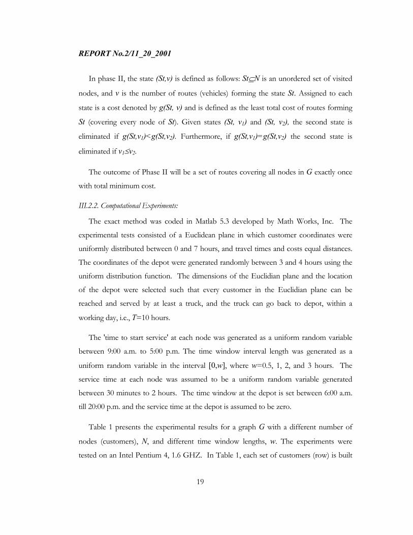
In phase II, the state (St,v) is defined as follows: St⊆N is an unordered set of visited

nodes, and v is the number of routes (vehicles) forming the state St. Assigned to each

state is a cost denoted by g(St, v) and is defined as the least total cost of routes forming

St (covering every node of St). Given states (St, v1) and (St, v2), the second state is

eliminated if g(St,v1)<g(St,v2). Furthermore, if g(St,v1)=g(St,v2) the second state is

eliminated if v1≤v2.

The outcome of Phase II will be a set of routes covering all nodes in G exactly once

with total minimum cost.

III.2.2. Computational Experiments:

The exact method was coded in Matlab 5.3 developed by Math Works, Inc. The

experimental tests consisted of a Euclidean plane in which customer coordinates were

uniformly distributed between 0 and 7 hours, and travel times and costs equal distances.

The coordinates of the depot were generated randomly between 3 and 4 hours using the

uniform distribution function. The dimensions of the Euclidian plane and the location

of the depot were selected such that every customer in the Euclidian plane can be

reached and served by at least a truck, and the truck can go back to depot, within a

working day, i.e., T=10 hours.

The 'time to start service' at each node was generated as a uniform random variable

between 9:00 a.m. to 5:00 p.m. The time window interval length was generated as a

uniform random variable in the interval [0,w], where w=0.5, 1, 2, and 3 hours. The

service time at each node was assumed to be a uniform random variable generated

between 30 minutes to 2 hours. The time window at the depot is set between 6:00 a.m.

till 20:00 p.m. and the service time at the depot is assumed to be zero.

Table 1 presents the experimental results for a graph G with a different number of

nodes (customers), N, and different time window lengths, w. The experiments were

tested on an Intel Pentium 4, 1.6 GHZ. In Table 1, each set of customers (row) is built

REPORT No.2/11_20_2001

20

upon the previous row. For instance, for the number of customers (nodes) equal to 10,

we used the same randomly generated customers for N=7 and added 3 newly generated

customers. At each row of Table 1, we used the same 'times to start service' at

customers’ locations while the time window interval lengths were generated randomly, as

described above. Table 1 also demonstrates the number of vehicles deployed at each

scenario to achieve the minimum cost.

Table 1: The exact method: computational experiments.

w=0.5 hour w=1 hour w=2 hours w=3 hours

No of nodes

Opt

imum

C

ost

CPU

tim

e5

No

Veh

icle

s

Opt

imum

C

ost

CPU

tim

e

No

Veh

icle

s

Opt

imum

C

ost

CPU

tim

e

No

Veh

icle

s

Opt

imum

C

ost

CPU

tim

e

No

Veh

icle

s

7 15.10 0.27 4 15.43 0.28 4 13.69 0.38 3 13.69 0.44 3

10 28.82 0.39 6 28.82 0.39 6 23.88 1.70 5 23.16 3.40 4

15 48.49 1.81 10 48.49 3.35 10 35.38 326.3 7 37.70 625.7 7

20 66.00 85.52 13 66.00 302.3 13 NAa NA NA NA NA NA

a) NA: The result couldn’t be obtained.

As shown in Table 1, for the first three sets of tests, where the problem size was

relatively small (around 15 nodes), the exact method was able to find the optimal

solution for all window sizes.

III.3. Genetic Algorithms for m-TSPTW

The exact method is applied to a few sets of problems as shown in Table 1. Since the

problem is NP-hard, the computational time for large size problems is fairly high. What

we observed in our computational experiments is the DP algorithm for the set covering

5 CPU time: is the time in seconds that has been used by the program to obtain the final result.

REPORT No.2/11_20_2001

21

problem (phase II) is computationally slow for problems involving around 20 or more

nodes.

Although the proposed method is capable of finding the exact solution for small size

problems, the algorithm becomes computationally very costly for problems of medium

or larger size. Hence, it is desirable to find a mechanism that results in a compromise

between the quality of the solution and the computational time needed to obtain that

solution. Meta-heuristic methods such as Tabu Search, Simulated Annealing (SA), and

Genetic Algorithms (GA) offer such a mechanism that forces the algorithm out of the

locally optimal solutions in their search for the globally optimal solution. These methods

have been recently considered and applied to Set Covering Problems (SCP) with

promising results, for instance see [1, 12, 17, 23].

Since it is computationally prohibitive to find the optimal solution among the feasible

set of solutions, we propose using a genetic algorithm for solving the second phase in

order to find an approximate solution for large size problems.

III.3.1. Methodology:

First, the sets of the routes found in Phase I are encoded in the form of matrix β

presented in ( 9 ). Matrix β is an n×m matrix, where n is the number of customers in

graph G and m is the number of the routes generated in phase I. Each element βij of this

matrix has a binary value, i.e., it is either one or zero. The βij is one if route j visits node

i∈N, and zero otherwise. Without loss of generality, we assume that the columns of β

are ordered in decreasing order of the number of ones in each column (nodes visited by

route j), and columns with equal number of ones are ordered in increasing order of cost.

Equation ( 10 ) illustrates a typical matrix β for a graph of 4 nodes where 11 feasible

routes were generated in Phase I.

REPORT No.2/11_20_2001

22

=

10001001010001001110110100110011100010010101

β ( 10 )

A solution to the set-covering problem is a set of routes that visited all customers

exactly once. Using the encoded representation of feasible routes in ( 10 ), a solution will

be a set of columns in matrix β, e.g. columns 2 and 8, such that the summation over the

rows of these columns generate a unit vector column, i.e., has the value one at every row.

We used an m-bit binary string, which will be called chromosome thereafter, to represent

a solution structure. A value 1 for the ith bit in the string implies that column i is in the

solution set. Equation ( 11 ) shows two typical solutions (chromosomes) obtained from

matrix β in ( 10 ).

]00000001100[1]00010000010[1

==

chrmchrm

( 11 )

To each chromosome a cost (fitness function) is associated which determines how

'good' each chromosome is. With binary representation, the fitness function ψj of

chromosome j can be simply calculated by

∑=

⋅=m

iijij F

1ρψ ( 12 )

where ρij is the value of the ith bit in the chromosome j, and Fi is the cost of

traveling on route i calculated in phase I.

The initial population of chromosomes is generated by randomly assigning feasible

route i to chromosome j. The route i is weighted more if it covers more of the remaining

nodes with less total costs. Among all population of chromosomes two are “selected”

REPORT No.2/11_20_2001

23

for generating a new chromosome (offspring). We used the binary tournament selection

method by forming two groups of chromosomes with equal number of chromosomes in

each group. The chromosomes are randomly placed in each group. One chromosome

from each group with the best fitness function is selected to produce an offspring.

Crossover and mutation operators are then applied on two selected chromosomes to

generate the offspring. Let’s assume that chromosomes j and k have been selected for

producing the offspring l. By applying the crossover operator, the value of ρil (the ith bit

in chromosome l) is set equal to ρij with probability p, which is equal to

,kj

jpψψ

ψ+

= ( 13 )

and to ρik with probability (1-p). Obviously, if the values of ρij and ρik are equal, the

value of ρil will be equal to this value, i.e., ρil=ρij=ρik. By applying the mutation operator,

the value of ρil will be inverted by some small probability q. However, the new generated

offspring, i.e. lth chromosome, may not be feasible. A heuristic method can be used to

make the chromosome feasible [1].

The newly generated offspring substitutes one of the chromosomes in the initial

population with a fitness function worse than the average fitness of all the population.

This procedure will continue till the termination criterion is met, which is a

predetermined number of iterations.

The GA algorithm is summarized as follows:

Step 1: Form matrix β; generate the initial population.

Step 2: Select two chromosomes for generating offspring.

Step 3: Apply the crossover operator.

REPORT No.2/11_20_2001

24

Step 4: Apply the mutation operator.

Step5: Make the offspring feasible.

Step 6: Calculate the fitness function associated to the offspring.

Step 7: Substitute one of the chromosome in the initial population with the

offspring.

Step 8: Repeat steps 2-8 until the termination criterion is met. The best

solution is the one with the minimum fitness function in the population.

It is worth mentioning that it is generally believed that GA is slow and would take

time to find a high quality solution [25]. The amount of computational effort required

by this algorithm depends on the size of the problem, i.e., the number of the nodes in

graph G (number of the rows in matrix β) and the number of the generated feasible

solutions in Phase I (number of the columns in matrix β).

III.3.2. Computational Experiments:

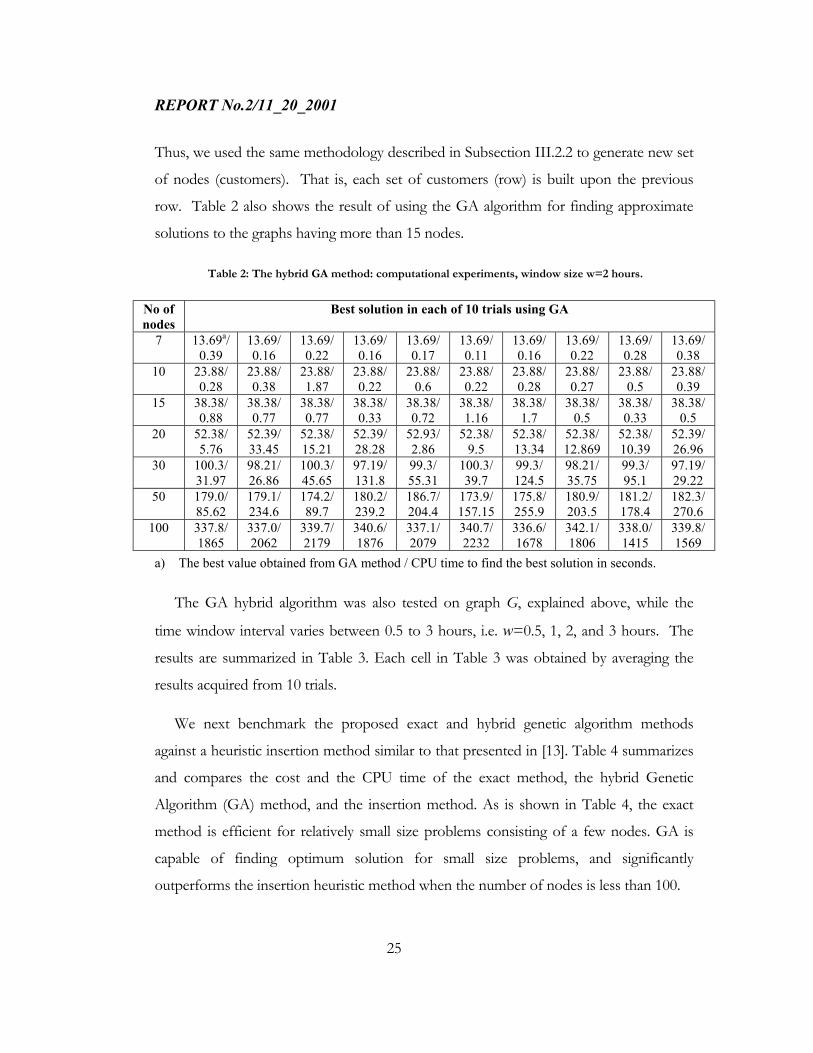
The hybrid GA method was also coded in Matlab 5.3. Table 2 shows the results of

using the hybrid GA method for finding the best solution among all feasible solutions

for different number of customers while the time window length, w, was set to 2 hours.

The top number in each cell of Table 2 is the value of the objective function, whereas

the lower number is the computational time to find the best solution in seconds, as

supplied by Matlab. The same data sets generated in Subsection III.2.2 were used here to

evaluate the efficiency of the GA method.

For each set of nodes, the genetic algorithm was applied 10 times in order to assess

the reliability and repeatability of the algorithm. A comparison of Table 1 and Table 2

indicates that the hybrid GA algorithm was able to find the optimum solution for 7, 10

and 15 number of nodes at every trial in a relatively short amount of time. These

promising results encouraged us to extend the number of nodes in graph G up to 100.

REPORT No.2/11_20_2001

25

Thus, we used the same methodology described in Subsection III.2.2 to generate new set

of nodes (customers). That is, each set of customers (row) is built upon the previous

row. Table 2 also shows the result of using the GA algorithm for finding approximate

solutions to the graphs having more than 15 nodes.

Table 2: The hybrid GA method: computational experiments, window size w=2 hours.

No of nodes

Best solution in each of 10 trials using GA

7 13.69a/ 0.39

13.69/ 0.16

13.69/ 0.22

13.69/ 0.16

13.69/ 0.17

13.69/ 0.11

13.69/ 0.16

13.69/ 0.22

13.69/ 0.28

13.69/ 0.38

10 23.88/ 0.28

23.88/ 0.38

23.88/ 1.87

23.88/ 0.22

23.88/ 0.6

23.88/ 0.22

23.88/ 0.28

23.88/ 0.27

23.88/ 0.5

23.88/ 0.39

15 38.38/ 0.88

38.38/ 0.77

38.38/0.77

38.38/ 0.33

38.38/ 0.72

38.38/ 1.16

38.38/ 1.7

38.38/ 0.5

38.38/ 0.33

38.38/ 0.5

20 52.38/ 5.76

52.39/ 33.45

52.38/ 15.21

52.39/ 28.28

52.93/ 2.86

52.38/ 9.5

52.38/ 13.34

52.38/ 12.869

52.38/ 10.39

52.39/ 26.96

30 100.3/ 31.97

98.21/ 26.86

100.3/ 45.65

97.19/ 131.8

99.3/ 55.31

100.3/ 39.7

99.3/ 124.5

98.21/ 35.75

99.3/ 95.1

97.19/ 29.22

50 179.0/ 85.62

179.1/ 234.6

174.2/ 89.7

180.2/ 239.2

186.7/ 204.4

173.9/ 157.15

175.8/ 255.9

180.9/ 203.5

181.2/ 178.4

182.3/ 270.6

100 337.8/ 1865

337.0/ 2062

339.7/ 2179

340.6/ 1876

337.1/ 2079

340.7/ 2232

336.6/ 1678

342.1/ 1806

338.0/ 1415

339.8/ 1569

a) The best value obtained from GA method / CPU time to find the best solution in seconds.

The GA hybrid algorithm was also tested on graph G, explained above, while the

time window interval varies between 0.5 to 3 hours, i.e. w=0.5, 1, 2, and 3 hours. The

results are summarized in Table 3. Each cell in Table 3 was obtained by averaging the

results acquired from 10 trials.

We next benchmark the proposed exact and hybrid genetic algorithm methods

against a heuristic insertion method similar to that presented in [13]. Table 4 summarizes

and compares the cost and the CPU time of the exact method, the hybrid Genetic

Algorithm (GA) method, and the insertion method. As is shown in Table 4, the exact

method is efficient for relatively small size problems consisting of a few nodes. GA is

capable of finding optimum solution for small size problems, and significantly

outperforms the insertion heuristic method when the number of nodes is less than 100.

REPORT No.2/11_20_2001

26

Table 3: The hybrid GA method: the summary of the computational experiments for different window size (based on the results of 10 trials).

w=0.5 hour w=1 hour w=2 hours w=3 hours No of nodes Best

Cost CPU time

Best Cost

CPU time

Best Cost

CPU time

Best Cost

CPU time

7 15.10 o 0.20 15.43 o 0.18 13.69 o 0.22 13.69 o 0.27

10 28.82 o 0.19 28.82 o 0.19 23.88 o 0.5 23.16 o 0.9

15 48.49 o 0.59 48.49 o 0.99 35.38 o 0.76 37.70 o 6.34

20 66.00 o 2.17 66.00 o 2.89 52.44 15.86 48.97 11.71

30 112.2 28.76 104.0 23.64 98.97 61.61 95.96 50.56

50 196.9 126.7 189.5 240.9 179.4 191.91 172.0 236.76

100 359.7 1234 352.4 1368 338.9 1876 329.5 1743

o) Optimum Value.

Table 4: Comparing exact, hybrid GA, and insertion methods, N=20 nodes, w=2 hours.

Dynamic Programming Genetic Algorithm a Insertion method No of nodes Cost CPU time Cost CPU time Cost CPU time

7 13.69 0.38 13.69 0.22 17.69 0.11

10 23.88 1.70 23.88 0.50 26.96 0.11

15 35.38 326.4 35.38 0.76 42.25 0.16

20 NAb NA 52.44 15.86 59.91 0.27

30 NA NA 98.97 61.61 107.0 0.49

50 NA NA 179.4 191.91 194.45 1.45

100 NA NA 338.9 1876 359.08 4.67

a) In average (based on the results of 10 trials). b) NA: The result couldn’t be obtained.

REPORT No.2/11_20_2001

27

It should be noted that in our computational experiments the maximum number of

generated solutions (offspring) in GA was limited to 1000. Obviously, by increasing this

number a better solution may be found.

IV. CONCLUSIONS

In this paper, we investigated the cargo movement in metropolitan areas adjacent to

marine ports. In particular, we were interested in improving the methods for truck

scheduling and route planning, where ISO containers need to be transferred between

marine terminals, intermodal facilities, and end customers. The objective was to reduce

empty miles, and to improve customer service. We showed that the container movement

by trucks can be modeled as an asymmetric multi-Traveling Salesmen Problem with

Time Windows (m-TSPTW). Moreover, we proposed two methodologies for solving the

m-TSPTW:

− An exact two-phase Dynamic Programming (DP), and

− A hybrid methodology consisting of DP in conjunction with genetic algorithms

(GA).

The results of our computational experiments indicate that the exact method was

efficient for relatively small size problems consisting of a few nodes. However, the

hybrid GA was capable of finding the optimum solution for small size problems and a

sub-optimum solution for medium to large size problems (more than 30 nodes).

Acknowledgments

We would like to thank Ms. Patty Senecal, Mr. Mike Johnson, and Mr. J.R. Barba of

Transport Express for supplying us with useful information on the problem.

References

[1] J.E. Beasley, P.C. Chu, A genetic algorithm for the set covering problem, European Journal of Operational Research, vol. 94, pp. 392-404, 1996.

REPORT No.2/11_20_2001

28

[2] L. Bodin, B. Golden, A. Assad, M. Ball, Routing and scheduling of vehicles and crews: the state of the art, Computers & Operations Research, vol.10, no.2, pp. 63-211, 1983.

[3] R.W. Cavo, A new heuristic for the traveling salesman problem with time windows, Transportation Science, vol. 34, no. 1, pp. 113-124, 2000.

[4] M. Desrochers, J. Desrosiers, M. Solomon, A new optimization algorithm for the vehicle routing problem with time windows, Operations Research, vol. 40, pp. 342-354, 1992.

[5] J. Desrosiers, Y. Dumas, M.M Solomon, F. Soumis, Time constrained routing and scheduling, in: M.O. Ball, T.L. Magnati, C.L. Monma, G.L. Nemhauser, (eds.) Network Routing, Handbooks in Operations Research and management Science, Volume 8, INFORMS, Elsevier Science, pp. 35-130, 1995.

[6] Y. Dumas, J. Desrosiers, E. Gelinas, M.M. Solomon, An optimal algorithm for the traveling salesman problem with time windows, Operations Research, vol. 43, no. 2, pp. 367-371, 1995.

[7] M. Fisher, “Vehicle routing,” in: M.O. Ball, T.L. Magnati, C.L. Monma, G.L. Nemhauser, (eds.) Network Routing, Handbooks in Operations Research and management Science, Volume 8, INFORMS, Elsevier Science, pp. 1-33, 1995.

[8] M.R. Garey, D.S. Johnson, Computers and Intractability: A Guide to the Theory of NP-Completeness, W.H. Freeman, San Francisco, 1979.

[9] M. Gendreau, A. Hertz, G. Laporte, M. Stan, A generalized insertion heuristic for the traveling salesman problem with time windows, Operations Research, vol. 43, no. 3, pp. 330-335, 1998.

[10] B.L. Golden, A.A. Assad, Vehicle Routing: Methods and Studies, North Holland Publication, Amsterdam 1988.

[11] R.W. Hall, C. Intihar, Commercial Vehicle Operations: Government Interfaces and Intelligent Transportation Systems, California PATH Research Report UCB-ITS-PRR-97-12, 1997.

[12] L.W. Jacobs, M.J. Brusco, A simulated annealing based heuristic for the set-covering problem, Proceedings of Decision Sciences Institute, vol. 2, pp. 1189-91, 1994.

[13] J.J. Jaw, A.R Odoni., H.N. Psaraftis, N.H.M. Wilson, A heuristic algorithm for the multi-vehicle advance request dial-a-ride problem with time windows, Transportation Research, vol. 20B, no. 3, pp. 243-257, 1986.

REPORT No.2/11_20_2001

29

[14] N. Kohl, J. Desrosiers, O.B.G. Madsen, M.M. Solomon, F. Soumis 2-path cuts for the vehicle routing problem with time windows, Transportation Science, vol. 33, no. 1, pp. 101-16, 1999.

[15] M.S. Lee, New Algorithms for the m-TSPTW, Ph.D. Thesis, University of Maryland Collage Park, 1992.

[16] S. Lin, B. Kernighan, An effective heuristic algorithm for the traveling salesman problem, Operations Research, vol. 1, pp. 498-516, 1973.

[17] L. Lorena, L.S. Lopes, Genetic algorithms applied to computationally difficult problems, Journal of Operational Research Society, vol. 48, pp. 440-445, 1997.

[18] Meyer, Mohaddes Associates, Inc., Gateway Cities Trucking Study. Gateway Cities Council of Governments Southeast Los Angeles County, 1996.

[19] L. Ng, R.L. Wessels, D. Do, F. Mannering, W. Barfield, Statistical Analysis of Commercial Driver and Dispatcher Requirements for Advanced Traveller Information Systems. Transportation Research-C, vol. 3, no.6, 353-369, 1995.

[20] G. Reinelt, The traveling salesman problem: computational solutions for TSP applications, Lecture Notes in Computer Science, Springer-Verlag, 1994.

[21] M.W.P. Savelsbergh, Local search in routing problems with time windows, Annals of Operations Research, vol. 4, no. 1-4, pp. 285-305, 1985.

[22] M.W.P Savelsbergh, N. Sol, The general pickup and delivery problem, Transportation Science, vol. 29, no. 1, pp. 17-29, 1995.

[23] S. Sen, Minimal cost set covering using probabilistic methods, Proceeding of 1993 ACM/SIGAPP Symposium of Applied Computing, pp. 157-164, 1993.

[24] M.J. Vickerman, Next-Generation Container Vessels: Impact on transportation Infrastructure an Operations, TR News, vol. 196, pp. 3-15, May-June, 1998.

[25] A.M.S. Zalzala, P.J. Fleming, Genetic Algorithms in Engineering Systems, IEE control Engineering Series 55, 1997.