contagion - leonid zhukov€¦ · contagion is said to occur if one action—say, action 1—can...

Review of Economic Studies (2000) 67, 57–78 0034-6527y00y00040057$02.00 2000 The Review of Economic Studies Limited

ContagionSTEPHEN MORRIS

Yale University

First version received February 1997; final version accepted August 1998 (Eds.)

Each player in an infinite population interacts strategically with a finite subset of that popu-lation. Suppose each player’s binary choice in each period is a best response to the populationchoices of the previous period. When can behaviour that is initially played by only a finite set ofplayers spread to the whole population? This paper characterizes when such contagion is possiblefor arbitrary local interaction systems. Maximal contagion occurs when local interaction is suffic-iently uniform and there is low neighbour growth, i.e. the number of players who can be reachedin k steps does not grow exponentially in k.

1. INTRODUCTION

When large populations interact strategically, players may be more likely to interact withsome players than others. A local interaction system describes a set of players and specifieswhich players interact with which other players. If in addition, each player at each locationhas a set of available actions and a payoff function from each of his various interactions,we have a local interaction game. The strategic problem becomes interesting when it isassumed that players cannot tailor their behaviour for each neighbour, but must choosea constant action for all neighbours.

A recent literature has examined such local interaction games.1 A key finding of thatanalysis is that local interaction may allow some forms of behaviour to spread in certaindynamic systems. For example, suppose that players are arranged along a line, and eachplayer interacts with his two neighbours. An action is 1

2-dominant if it is a best responsewhen a player has at least one neighbour playing that action.2 Ellison (1993) showed thatif an action was 1

2-dominant at every location and was played at any pair of neighbouringlocations, then best response dynamics alone would ensure that it would eventually beplayed everywhere.3

A number of papers have explored how robust this type of phenomenon is to thestructure of the local interaction. For example, two-dimensional lattices have been muchstudied (Anderlini and Ianni (1995), Blume (1995), Ellison (2000)). Blume (1995) con-sidered local interaction systems where locations are on an m-dimensional lattice and thereis a translation invariant description of the set of neighbours. Unfortunately, it is hard toknow what to make of results which rely on a particular geometric structure. It is not

1. The relevant pure game theory literature includes Anderlini and Ianni (1996), Berninghaus andSchwalbe (1996a, 1996b), Blume (1993, 1995), Ellison (1993, 2000), Goyal (1996), Galeshoot and Goyal (1997),Ianni (1997), Mailath, Samuelson and Shaked (1997a) and Young (1998, Chapter VI). See Durlauf (1997) for asurvey of the closely related economics literature on local interaction. This paper follows those literatures intaking the local interaction system as exogenous. See Ely (1997) and Mailath, Samuelson and Shaked (1997b)for models with endogenous local interaction.

2. If there are only two possible actions in a symmetric two player game, both players choosing the 12-

dominant action is risk dominant in the sense of Harsanyi and Selten (1988).3. Ellison (1993) and much of the literature cited above are concerned with stochastic versions of best

response dynamics; as I discuss briefly in Section 7, some of the conclusions are driven by properties of determin-istic best response dynamics.

57

ps322$p827 10-02-:0 14:13:03

58 REVIEW OF ECONOMIC STUDIES

clear that the study of lattices will explain which qualitative features of neighbourhoodrelations determine strategic behaviour.

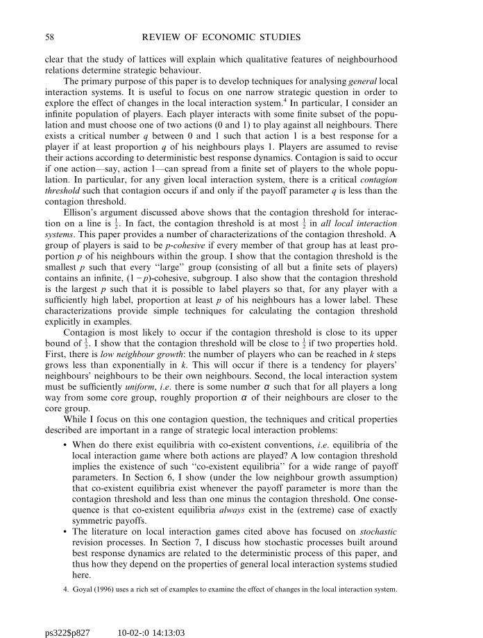
The primary purpose of this paper is to develop techniques for analysing general localinteraction systems. It is useful to focus on one narrow strategic question in order toexplore the effect of changes in the local interaction system.4 In particular, I consider aninfinite population of players. Each player interacts with some finite subset of the popu-lation and must choose one of two actions (0 and 1) to play against all neighbours. Thereexists a critical number q between 0 and 1 such that action 1 is a best response for aplayer if at least proportion q of his neighbours plays 1. Players are assumed to revisetheir actions according to deterministic best response dynamics. Contagion is said to occurif one action—say, action 1—can spread from a finite set of players to the whole popu-lation. In particular, for any given local interaction system, there is a critical contagionthreshold such that contagion occurs if and only if the payoff parameter q is less than thecontagion threshold.

Ellison’s argument discussed above shows that the contagion threshold for interac-tion on a line is 1

2 . In fact, the contagion threshold is at most 12 in all local interaction

systems. This paper provides a number of characterizations of the contagion threshold. Agroup of players is said to be p-cohesive if every member of that group has at least pro-portion p of his neighbours within the group. I show that the contagion threshold is thesmallest p such that every ‘‘large’’ group (consisting of all but a finite sets of players)contains an infinite, (1Ap)-cohesive, subgroup. I also show that the contagion thresholdis the largest p such that it is possible to label players so that, for any player with asufficiently high label, proportion at least p of his neighbours has a lower label. Thesecharacterizations provide simple techniques for calculating the contagion thresholdexplicitly in examples.

Contagion is most likely to occur if the contagion threshold is close to its upperbound of 1

2 . I show that the contagion threshold will be close to 12 if two properties hold.

First, there is low neighbour growth: the number of players who can be reached in k stepsgrows less than exponentially in k. This will occur if there is a tendency for players’neighbours’ neighbours to be their own neighbours. Second, the local interaction systemmust be sufficiently uniform, i.e. there is some number α such that for all players a longway from some core group, roughly proportion α of their neighbours are closer to thecore group.

While I focus on this one contagion question, the techniques and critical propertiesdescribed are important in a range of strategic local interaction problems:

• When do there exist equilibria with co-existent conventions, i.e. equilibria of thelocal interaction game where both actions are played? A low contagion thresholdimplies the existence of such ‘‘co-existent equilibria’’ for a wide range of payoffparameters. In Section 6, I show (under the low neighbour growth assumption)that co-existent equilibria exist whenever the payoff parameter is more than thecontagion threshold and less than one minus the contagion threshold. One conse-quence is that co-existent equilibria always exist in the (extreme) case of exactlysymmetric payoffs.

• The literature on local interaction games cited above has focused on stochasticrevision processes. In Section 7, I discuss how stochastic processes built aroundbest response dynamics are related to the deterministic process of this paper, andthus how they depend on the properties of general local interaction systems studiedhere.

4. Goyal (1996) uses a rich set of examples to examine the effect of changes in the local interaction system.

ps322$p827 10-02-:0 14:13:03

MORRIS CONTAGION 59

This paper builds on two literatures. The questions studied and the formal frameworkused are very close to the earlier literature on local interaction games (see Footnote 1).When applied to lattice examples, the contribution of this paper is to provide a usefullanguage for discussing the structure of local interaction that can be used to generalizearguments already used in that literature (especially, those of Blume (1995)). But muchmore importantly, this approach allows a discussion of the key qualitative properties oflocal interaction systems that does not rely on special features of lattices.

The inspiration for this work is an apparently unrelated literature on the role ofhigher-order beliefs in incomplete information games. It is possible to show a formalequivalence between local interaction games and incomplete information games. The for-mal techniques in this paper are then analogues of the belief operator techniques, intro-duced by Monderer and Samet (1989), and used in the higher-order beliefs literature.5

However, this relationship is explored in detail in a companion piece (Morris (1997b)), soin this paper, the ideas are developed independently.

The paper is organized as follows. Local interaction games are introduced, and con-tagion threshold defined, in Section 2. Some examples are discussed in Section 3; theseillustrate the questions studied but also highlight the risks of taking simple interactionsystems too seriously. The crucial general properties of interaction systems are introducedand discussed in Section 4. The main results—characterizations of the contagion thresh-old—are presented in Section 5. Section 6 presents the results on the co-existence of con-ventions. Various ways of adding random elements to this paper’s deterministic dynamicare discussed in Section 7. Section 8 concludes.

2. LOCAL INTERACTION GAMES

A local interaction game consists of a local interaction system describing how playersinteract and their payoffs from those interactions.

A local interaction system consists of an infinite population, each of whom interactswith a finite subset of the population.6 So fix a countably infinite set of players X and let∼ be a binary relation on X. If x′∼x, say that ‘‘x′ is a neighbour of x.’’ The followingare assumed, for all x, x′∈X ,

1. Irreflexivity: xïx. No player is his own neighbour.2. Symmetry: x′∼x ⇒ x∼x′. If x′ is a neighbour of x, then x is a neighbour of x′.3. Bounded Neighbours: there exists M such that #{y∈X : y∼x}oM. Each player has

at most M neighbours.4. Connectedness: there exist {x1 , x2 , . . . , xK}⊆ X such that x1Gx′, xKGx and

xk∼xkC1 for each kG1, . . . , KA1. There is some path connecting any pair ofplayers.

A local interaction system is a pair (X , ∼ ), where ∼ satisfies properties [1] through [4].7

Write Γ(x) for the set of neighbours of x, i.e. Γ(x)≡{x′: x′∼x}; a group of players, X, is

5. The papers of Monderer and Samet (1989, 1996), Morris, Rob and Shin (1995) and Kajii and Morris(1997) are especially relevant.

6. The assumption of an infinite population is for analytic convenience. Analogous results could be provenfor large finite populations, although some of the simplicity of the results would be lost.

7. Irreflexivity and Symmetry imply that (X , ∼ ) is an (infinite) graph. Bounded Neighbours implies thateach player has a small number of neighbours (i.e. finite) relative to the whole (infinite) population. Connec-tedness is assumed for convenience only; if the graph were disconnected, the paper’s results could be applied toeach connected component. Symmetry is a substantive assumption, necessary for many of the results that follow.It will imply that if player 1 cares about player 2’s action, then player 2 must care about player 1’s action.

ps322$p827 10-02-:0 14:13:03


an arbitrary subset of X ; the complementary group of X in X is written as Xr , i.e. Xr G{x∈X : x∉X}.

Each player has two possible actions, 0 and 1. Write u(a, a′ ) for the payoff of a playerfrom a particular interaction if he chooses a and his neighbour chooses a′. This payofffunction corresponds to symmetric payoff matrix:

0 1

0 u(0, 0), u(0, 0) u(0, 1), u(1, 0) ·

1 u(1, 0), u(0, 1) u(1, 1), u(1, 1)

It is assumed that this game has two strict Nash equilibria, so that u(0, 0)Hu(1, 0) andu(1, 1)Hu(0, 1). However, for the analysis of this paper, only the best response correspon-dence matters. In particular, observe that action 1 is best response for some player exactlyif he assigns probability at least

qGu(0, 0)Au(1, 0)

(u(0, 0)Au(1, 0))C(u(1, 1)Au(0, 1))

to the other player choosing action 1. Thus payoffs are parameterized by the criticalprobability q∈(0, 1). All analysis in the paper is unchanged if we restrict attention to thepayoff matrix

0 1

0 q, q 0, 0 (2.1)·

1 0, 0 1Aq, 1Aq

Now a local interaction game is a 3-tuple (X , ∼ , q).A conventional description of best responses would proceed as follows. A (pure)

configuration is a function s: X →{0, 1}. Given configuration s, player x’s best response isto choose an action which maximizes the sum of his payoffs from his interactions witheach of his neighbours. Thus action a is a best response to configuration s for player x,i.e. a∈b(s, x), if

∑y∈Γ (x) u(a, s ( y))n∑y∈Γ (x) u(1Aa, s( y)).

Configuration s′ is a best response to configuration s if s′(x) is a best response to s foreach x, i.e. if s′(x)∈b(s, x) for all x∈X .

But notice that action 1 is a best response for a player if at least proportion q of hisneighbours choose action 1; and action 0 is a best response if at least proportion 1Aq ofhis neighbours choose action 0. So it is convenient to describe configurations of play andbest responses as follows. Identify a configuration with the group of players who chooseaction 1 in that configuration. Thus configuration s is identified with the group XG{x: s(x)G1}; group X is identified with configuration s where

s(x)G51,

0,

if x∈X

if x∉X.

ps322$p827 10-02-:0 14:13:03

MORRIS CONTAGION 61

Now let π [X ux] be the proportion of x’s neighbours who are in group X, i.e.

π [X ux]G# (X∩Γ(x))

#Γ(x).

Write Πp (X ) for the players for whom at least proportion p of their interactions are withplayers in X, i.e.

Πp (X )G{x∈X : π [X ux]np}.

In this notation, X is a best response to Y if X⊆Πq(Y ) and Xr ⊆Π1Aq(Yr ). For simplicity, Iassume the tie-breaking rule that action 1 is chosen if a player is indifferent between thetwo actions. Thus Πq (X ) will be referred to as the best response to X. This tie-breakingrule makes no difference to the contagion results, except for non-generic values of q.8

This paper is concerned with the following question. Does there exist a finite groupof players, such that if that group starts out playing some action (say, without loss ofgenerality, action 1), best response dynamics will ensure that that action is eventuallyplayed everywhere? If so, action 1 spreads contagiously. The contagion threshold ξ isdefined to be the largest q for which such contagious dynamics are possible.

Definition 1. The contagion threshold, ξ, of local interaction system (X , ∼ ) is thelargest q such that action 1 spreads by best response dynamics from some finite group tothe whole population, i.e.9

ξGmax {q:*kn1 [Πq ]k (X )GX for some finite X}.

3. EXAMPLES

The examples described in this section provide some intuition for the contagion threshold(as well as fixing the notation described in the previous section). For each example, I state(without proof) the contagion threshold. Techniques described in Section 5 are later usedto establish these results. The examples will also be used to illustrate the critical graphtheoretic properties of interaction described in the next section. I write Z for the set ofintegers.

Example 1: Interaction on a line. The population is arranged on a line and eachplayer interacts with the player to his left and the player to his right. See Figure 1. Thisis represented formally as follows:

• X GZ ; x′∼x if x′GxA1 or x′GxC1.

If qF12 in the payoff matrix (2.1), action 1 is a best response whenever at least one

FIGURE 1

8. For generic values of q (in particular, as long as q≠nym for all integers nomoM ), π [X ux]≠q for allx∈X and X⊆X . In this case, Πq (X )GΠ1Aq (Xr ) for all X⊆X (so there is a unique best response always) andthus the tie-breaking rule does not matter. Section 7.1 describes the precise sense in which the tie-breaking ruledoes not matter.

9. The maximum can be shown to always exist, using the continuity properties of the operator Πp

described in Lemma 1 in the Appendix.

ps322$p827 10-02-:0 14:13:03


neighbour chooses action 1. Thus if two neighbours x and xC1 initially choose action 1,players xA1, x, xC1 and xC2 must all choose action 1 in the next period, players xA2,xA1, x, xC1, xC2 and xC3 must all choose action 1 in the period after that, and so on.So action 1 eventually spreads to the whole population. But if qH1

2 , no player switchesto action 1 unless both neighbours are already choosing 1. Thus the contagion thresholdis 1

2 .

Example 2: Nearest neighbour interaction in m dimensions. More generally, we canimagine the population situated on an m-dimensional lattice. Each player interacts withall players who are immediate neighbours in the lattice, i.e. whose coordinates differ inonly one dimension. If mG1, then we have the interaction on a line of the previousexample. See Figure 2 for the case where mG2.

• X GZm; x′∼x if ∑m

iG1 ux′iAxi uG1.

In this case, each player has 2m neighbours. The contagion threshold is 12m (i.e.

contagion occurs if and only if qo12m). Thus it appears that as interaction becomes ‘‘rich-

er’’ (i.e. as the number of dimensions increases) contagion becomes impossible. However,the next example suggests that this conclusion is premature.

Example 3: n-max distance interaction in m dimensions. The population is againsituated on an infinite m dimensional lattice. Each player interacts with all players whoare less than n steps away in each of the m dimensions. See Figure 3 for the case wheremG2 and nG1.

• X GZm; x′∼x if 1o maxiG1,...,m ux′mAxm uon.

The contagion threshold is n(2nC1)mA1y(2nC1)mA1. Table 1 gives the values of thisexpression for different values of m and n.

This example illustrates the lack of robustness of the nearest neighbour analysis. Ifwe simply add players at one diagonal remove (holding nG1), then increasing the numberof dimensions (m) never lowers the contagion threshold below 1

3; If we fix the number ofdimensions (m) and increase the radius of interaction (n), the contagion threshold tendsto 1

2 .

FIGURE 2

ps322$p827 10-02-:0 14:13:03

MORRIS CONTAGION 63

FIGURE 3

1 2 3 · n · n→S

1 12

12

12 · 1

2 · 12

2 38

512

716 ·

n(2nC1)

(2nC1)2A1 · 12

926

2562

147342 ·

n(2nC1)2

(2nC1)3A1123 ·

· · · · · · · · ·3mA1

3mA1

n(2nC1)mA1

(2nC1)mA112· ·m

2·5mA1

5mA1

3·7mA1

7mA1

· · · · · · · ·

M→S 13

25

37 ·

n

2nC1 · 12

TABLE 1

Example 4: Regions. The population is divided into an infinite number of ‘‘regions’’of m players each. Each player in a region interacts with every other player in that region.The regions are arranged in a line and each player also interacts with one player in eachneighbouring region. See Figure 4 for the case where mG3.

• X GZ B{1, . . . , m}; x′∼x if either (i) x′1Gx1 ; or (ii) ux′1Ax1 uG1 and x′2Gx2 .

The contagion threshold is 1y(mC1).

FIGURE 4

ps322$p827 10-02-:0 14:13:03


FIGURE 5

Example 5: Hierarchy. The population is arranged in a hierarchy. Each player hasm subordinates. Each player, except the root player, has a single superior. See Figure 5for the case where mG2.

• X G*S

kG0 Xk , where X0G{∅} and XkG{1, . . . , m}k for all kn1, with mn2;

x∼y if and only if xG( y, n) or yG(x, n) for some n∈{1, . . . , m}.

The contagion threshold is again 1y(mC1).

4. PROPERTIES OF INTERACTION

Three types of properties important in local interaction systems are described in thissection.

4.1. Cohesion

One natural measure of the ‘‘cohesion’’ of a social group is the relative frequency of tiesamong group members compared to non-members.10 For any given group of players X,do players in the group mostly interact with players within the group or with playersoutside the group? Let the cohesion of group X be the smallest p such that each player inX has proportion p of his interactions within X, i.e.

c(X )Gminx∈X

π [X ux]Gmax {p: X⊆Πp(X )}.

The minimum and maximum exist since, for all players x and groups X, π [X ux] is arational number with denominator less than or equal to M.

Definition 2. Group X is p-cohesive if c(X )np.

We can use the examples of the previous section to illustrate this concept.

• Example 1: Interaction on a line. Any non-trivial group (non-empty and not equalto the whole population) is at most 1

2-cohesive, since at least one player must haveone neighbour outside the group. For example, consider the group of players

10. Wasserman and Faust (1994, Chapter 7), identify four independent concepts of cohesion in the soci-ology literature: (i) the relative frequency of ties among group members compared to non-members [the notionstudied here]; (ii) the mutuality of ties; (iii) the closeness or reachability of members; and (iv) the frequency ofties among members.

ps322$p827 10-02-:0 14:13:03

MORRIS CONTAGION 65

{1, . . . , N} for some very large N. Most players have all of their interactions withinthe group. But the cohesion of the group is only 1

2 , because of the two criticalplayers, 1 and N, who have only 1

2 their interactions with the group.

• Example 2: Nearest neighbour interaction in m dimensions. Any group consistingof all players above some horizontal plane (i.e. taking the form {x∈Zm: x1nc})will be (2mA1)y2m-cohesive.

• Example 3: n-max distance in m dimensions. Any group consisting of all playersabove some horizontal plane (i.e. taking the form {x∈Zm: x1nc}) will be[(nC1)(2nC1)mA1A1]y[(2nC1)mA1]-cohesive. To see why, consider a player x withx1Gc. He has (2nC1)mA1A1 neighbours with first coordinate c; he hasn(2nC1)mA1 neighbours with first co-ordinate greater than c; and he hasn(2nC1)mA1 neighbours with first co-ordinate less than c. Thus proportion[(nC1)(2nC1)mA1A1]y[(2nC1)mA1] of his neighbours have first co-ordinategreater than or equal to c.

• Example 4: Regions. A pair of neighbouring regions (i.e. a group of the form {x∈Z B{1, . . . , m}: x1Gc or cC1}) is my(mC1)-cohesive, since each player in thatgroup has m neighbours within that group, and one neighbour outside.

• Example 5: Hierarchy. Any group consisting of all direct or indirect subordinatesof some player x∈X n , i.e. taking the form

{x∈*n′nn X n′ : xkGxk for each kG1, . . . , n},

will be my(mC1)-cohesive. To see why, note that player x has all neighbours excepthis superior in that group, while all other players in the group have all their neigh-bours in the group.

4.2. Weak links, strong links and neighbour growth

Granovetter (1973) introduced the distinction between ‘‘weak’’ and ‘‘strong’’ social links.11

Strong social links are often transitive: if A is a close friend of B and B is a close friendof C, then B and C are more likely to be close friends than two randomly chosen individ-uals. This ‘‘neighbour correlation’’ will be less pronounced the weaker the social link beingstudied.

In this section, I introduce a natural way of capturing this distinction for the infinitegraphs studied in this paper. Fix an individual, and calculate the number of players thatcan be reached in no more than n steps from that individual. If there is no neighbourcorrelation in the graph (i.e. links are weak), then the numbers of players reached willgrow exponentially. But if a significant proportion of players’ neighbours’ neighbours aretheir own neighbours, then this will tend to slow down the exponential growth. We willbe interested in the case where there is enough neighbour correlation to preventexponential growth.

The Erdos distance between player x and group X is n if it takes at most n steps toreach x from X; i.e. writing Γn(X ) for the set of players within Erdos distance n, Γ0(X )GX and ΓnC1(X )GΓn(X )∪{x′: x′∼x for some x∈Γn(X )}.

11. I am grateful to Michael Chwe for bringing this literature to my attention. See Chwe (2000) for moreon the strategic implications of different kinds of social links.

ps322$p827 10-02-:0 14:13:03


Definition 3. Local Interaction System (X, ∼ ) satisfies low neighbour growth ifγ −n#Γn(X )→0 as n→S, for all finite groups X and γ H1.12

In the hierarchy example, #Γ1(X0)G1Cm, #Γ2(X0)G1CmCm2, etc., so that

#Γ k(X0)G(1CmC· · ·Cmn)G(mnC1A1)y(mA1).

Thus the low neighbour growth property is not satisfied. In all the other examples con-sidered in Section 3, #Γn(X ) is a polynomial function of n, and thus low neighbour growthis satisfied.

Researchers in the sociology literature have empirically verified that #Γn(X ) growsslower for graphs describing more important relationships.13 To get a feel for the growthof #Γn(X ), consider the experimental finding of Milgram (1967) that the median Erdosdistance (derived from the relation ‘‘personally acquainted’’) between two randomlychosen individuals in the U.S. was five. To interpret this finding, consider two extremecases. The U.S. population at the time was around 200 million and Milgram estimatedthat each individual had approximately 500 acquaintances. Suppose that one individualhas no overlap between his acquaintances, his acquaintances’ acquaintances and hisacquaintances’ acquaintances’ acquaintances. Then over half the population would bewithin Erdos distance 3 of this individual (5003G125,000,000). On the other hand, sup-pose the population of 200 million was arranged in a circle and each individual knew 250people on either side, the median Erdos distance would be 200,000.

4.3. δ -Uniformity

The last property considered is more technical and requires some additional notation. Alabelling of players X is a bijection l: Z ++→X . Write L for the set of labellings and α l (k)for the proportion of neighbours of player l (k) who have a lower label under labelling l,i.e.

α l (l )G#{ j: l ( j )∼ l (k) and jFk}

#{ j : l ( j )∼ l (k)}.

Labelling l is an Erdos labelling if there exists a finite group X such that l (i)∈Γn(X ) andl ( j )∉Γn(X ) ⇒ iFj.

Definition 4. Local Interaction System (X, ∼ ) satisfies δ -uniformity if there exists anErdos labelling l such that for all sufficiently large K,

maxk′,knK

uα l (k′ )Aα l (k)uoδ . (4.1)

This seems to be a weak property. There must be some way of labelling players,consistent with Erdos distance from some finite group X, such that for players sufficiently

12. In fact, requiring the definition to hold ‘‘for all’’ finite X is redundant: if it holds for any finite X, itholds for all finite X. To see why, suppose that for some finite X and γ H1, γ −k#Γ k (X )HεH0, for infinitelymany k (i.e. γ −k#Γ k (X )→y 0). Fix any finite group Y. By connectedness, X⊆Γn (Y ) for some n. Now Γ k (X )⊆ΓnCk (Y), so γ −(nCk)#ΓnCk (Y )Hεγ −nH0 for infinitely many k, i.e. γ −k#Γ k (Y )→y 0.

13. In one classic study, Rapoport and Horvarth (1961) examined levels of friendship among junior highschool students. In a graph based on seventh and eighth best friends, #Γn(X ) grows fast. In a graph based onbest and second best friends, #Γn(X ) grows much more slowly.

ps322$p827 10-02-:0 14:13:03

MORRIS CONTAGION 67

FIGURE 6

far away from X, the proportion of neighbours with lower labels tends (roughly) to some-thing (with no restrictions on what that something is). Two examples illustrate theproperty.

• Example 5: Hierarchy. 0-uniformity is satisfied. Consider any Erdos labelling withinitial (singleton) group X0 . Now Γn(X0)G*

n

jG0 Xj . For any k, player l (k) hasexactly one neighbour with a lower label. Thus α l (k)G1y(mC1) for all k.

• Example 2: Nearest neighbour interaction in 2 dimensions. For any δF14 , δ -uni-

formity fails. Consider any Erdos labelling l. For any n, there are 4(nC1) playerswho are contained in ΓnC1({x}) but not Γn({x}) (see Figure 6). Those locationsform an empty square with nC2 players on each side; now 4n of those locations(those not on the corners) have α l (k)G

12 . But the four corners have α l (k)G

14 .

The latter example illustrates how δ -uniformity fails because of the lumpiness of thelattice. With sufficiently large neighbourhoods on a lattice, δ -uniformity is satisfied forsmall δ .

5. CHARACTERIZATIONS OF THE CONTAGION THRESHOLD

Recall that the contagion threshold, for a given local interaction system (X , ∼ ), wasdefined as follows

ξGmax {q:*kn1 [Πq ]k (X )GX for some finite X}.

Note that operator Πp is non-monotonic: X may contain Πp(X ), X may be contained inΠp(X ), or neither might be true. It is useful to analyse instead the following monotonicoperator

Πp+ (X )≡X∪Πp(X ).

It is straightforward to construct examples where X is finite, *kn1 [Πp ]k (X ) is finite, but*kn1 [Πp

+ ] k (X )GX . But it turns out that it must then be possible to find another,possibly larger but still finite, group Y with *kn1 [Πp ]k (Y )GX . This means that the

ps322$p827 10-02-:0 14:13:03


same contagion threshold arises if the monotonic operator Πq+ is substituted in the defi-

nition of the contagion threshold, i.e. ξ also equals

max {q:*kn1 [Πq+ ] k (X )GX for some finite X}.

This equivalence result is key to the characterizations that follow. It and the followingtwo propositions are proved in the Appendix.

Proposition 1. The contagion threshold is the smallest p such that every co-finite groupcontains an infinite, (1Ap)-cohesive, subgroup.14

Fix the parameter q in the payoff matrix (2.1). How can contagion be prevented?Suppose that there is a (1Ap)-cohesive group, with pFq, where action 0 is played initially.Since each player in that group has more than proportion 1Aq of his neighbours playing0, no player in that group will ever switch away from that group. So a sufficient conditionfor no contagion is that for any finite initial group X, the complement of X contains a(1Ap)-cohesive group, for some pFq. This sufficient condition turns out to be necessaryalso, and we get Proposition 1.

Proposition 2. The contagion threshold is the largest p such that under some labellingl, α l (k)np for all sufficiently large k. Formally

ξGmaxi∈L

1 limK→S

1minknK

α l (k)22 . (5.1)

That is, roughly speaking, the contagion threshold is the largest p such that we canlabel the players such that at least proportion p of all players’ neighbours have a lowerlabel (except for some initial group).

The following immediate corollaries of Propositions 1 and 2 respectively areespecially useful in identifying contagion thresholds in practice.

Corollary 1. [Upper Bound ]. If every co-finite group contains an infinite, (1Ap)-cohes-ive, subgroup, then ξop.

Corollary 2. [Lower Bound I ]. If there exists a labelling l with α l (k)np for all suffic-iently large k, then ξnp.

An even simpler lower bound is a consequence of Corollary 2. Recall that M was anupper bound on the number of possible neighbours.

Corollary 3. [Lower Bound II ]. The contagion threshold ξ is at least 1yM.

These corollaries can be used to establish the contagion threshold in earlier examples.

• Example 2: Nearest neighbour interaction in m dimensions. Every co-finite groupcontains an infinite (2mA1)y2m -cohesive group of the form {x∈Zm: x1nc}, so (byCorollary 1) ξo1y2m . But ξn1y2m by Corollary 3.

14. A group X is co-finite if its complement Xr is co-finite.

ps322$p827 10-02-:0 14:13:03

MORRIS CONTAGION 69

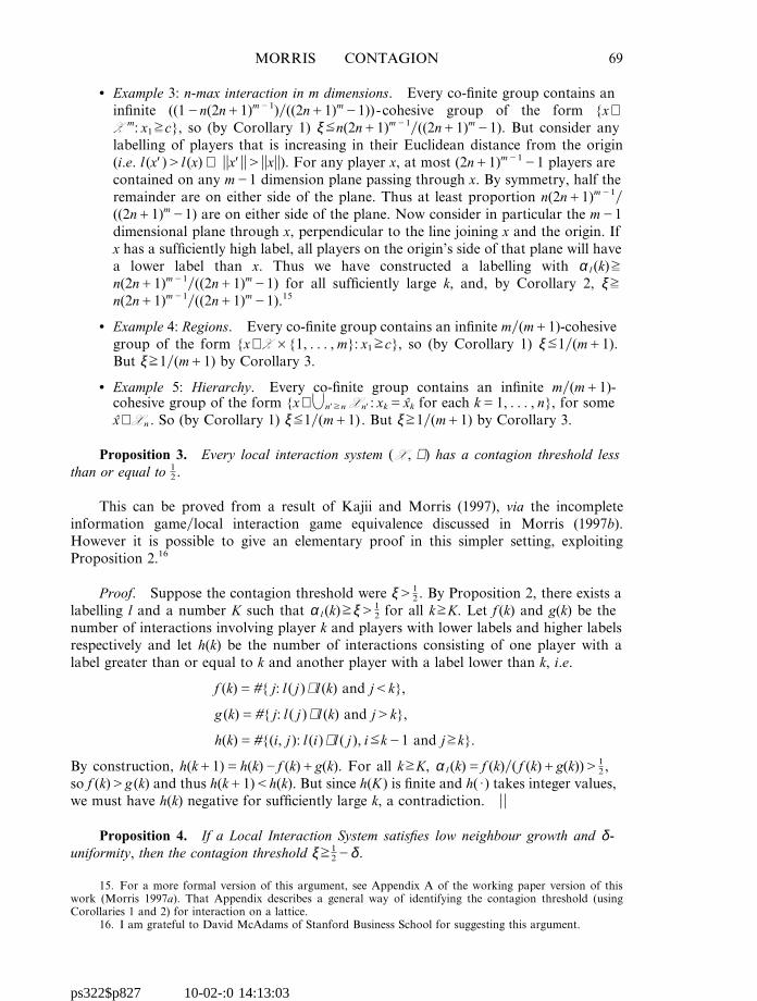
• Example 3: n-max interaction in m dimensions. Every co-finite group contains aninfinite ((1An(2nC1)mA1)y((2nC1)mA1))-cohesive group of the form {x∈Z

m: x1nc}, so (by Corollary 1) ξon(2nC1)mA1y((2nC1)mA1). But consider anylabelling of players that is increasing in their Euclidean distance from the origin(i.e. l (x′ )Hl (x) ⇒ uux′ uuHuuxuu). For any player x, at most (2nC1)mA1A1 players arecontained on any mA1 dimension plane passing through x. By symmetry, half theremainder are on either side of the plane. Thus at least proportion n(2nC1)mA1y((2nC1)mA1) are on either side of the plane. Now consider in particular the mA1dimensional plane through x, perpendicular to the line joining x and the origin. Ifx has a sufficiently high label, all players on the origin’s side of that plane will havea lower label than x. Thus we have constructed a labelling with α l (k)nn(2nC1)mA1y((2nC1)mA1) for all sufficiently large k, and, by Corollary 2, ξnn(2nC1)mA1y((2nC1)mA1).15

• Example 4: Regions. Every co-finite group contains an infinite my(mC1)-cohesivegroup of the form {x∈Z B{1, . . . , m}: x1nc}, so (by Corollary 1) ξo1y(mC1).But ξn1y(mC1) by Corollary 3.

• Example 5: Hierarchy. Every co-finite group contains an infinite my(mC1)-cohesive group of the form {x∈*n′nn X n′ : xkGxk for each kG1, . . . , n}, for somex∈X n . So (by Corollary 1) ξo1y(mC1). But ξn1y(mC1) by Corollary 3.

Proposition 3. Every local interaction system (X , ∼ ) has a contagion threshold lessthan or equal to 1

2 .

This can be proved from a result of Kajii and Morris (1997), via the incompleteinformation gameylocal interaction game equivalence discussed in Morris (1997b).However it is possible to give an elementary proof in this simpler setting, exploitingProposition 2.16

Proof. Suppose the contagion threshold were ξH12 . By Proposition 2, there exists a

labelling l and a number K such that α l (k)nξH12 for all knK. Let f (k) and g(k) be the

number of interactions involving player k and players with lower labels and higher labelsrespectively and let h(k) be the number of interactions consisting of one player with alabel greater than or equal to k and another player with a label lower than k, i.e.

f (k)G#{ j: l ( j )∼ l (k) and jFk},

g (k)G#{ j: l ( j )∼ l (k) and jHk},

h(k)G#{(i, j ): l (i)∼ l ( j ), iokA1 and jnk}.

By construction, h(kC1)Gh(k)Af (k)Cg(k). For all knK, α l (k)Gf (k)y( f (k)Cg(k))H12 ,

so f (k)Hg (k) and thus h(kC1)Fh(k). But since h(K ) is finite and h( · ) takes integer values,we must have h(k) negative for sufficiently large k, a contradiction. u u

Proposition 4. If a Local Interaction System satisfies low neighbour growth and δ -uniformity, then the contagion threshold ξn1

2Aδ .

15. For a more formal version of this argument, see Appendix A of the working paper version of thiswork (Morris 1997a). That Appendix describes a general way of identifying the contagion threshold (usingCorollaries 1 and 2) for interaction on a lattice.

16. I am grateful to David McAdams of Stanford Business School for suggesting this argument.

ps322$p827 10-02-:0 14:13:03


Blume (1995) showed that if players interact on a two dimensional lattice in suffic-iently large symmetric neighbourhoods, then the contagion threshold is close to 1

2 .17 Prop-

osition 4 generalizes Blume’s result to arbitrary interaction structures.

Proof. Suppose Erdos labelling l satisfies (4.1). Then there exist α and K with

αAδo#{ j: l ( j )∼ l (k) and jFk}

#{ j : l ( j )∼ l (k)}oα ,

for all knK. By Corollary 2, ξnαAδ . So if αn12 , we are done. Suppose then that αF1

2 .Now

#{ j : l ( j )∼ l (k) and jFk}o1 α1Aα2#{ j: l ( j )∼ l (k) and jHk}, (5.2)

for all knK. Since l is an Erdos labelling, there exists a finite group X such that l (i)∈Γn(X ) and l ( j )∉Γn(X ) ⇒ iFj. Let X0GX and XnGΓn(X )∩ΓnA1(X ) for nG1, 2, . . . .Choose N such that l (K )∈XNA1 . Now if nnN, summing equation (5.2) across all k withl (k)∈Xn implies

5#{( j, k): l ( j )∼ l (k), l ( j )∈XnA1 and l (k)∈Xn}

C#{( j, k): l ( j )∼ l (k), {l ( j ), l (k)}⊆Xn and jFk}6o1 α

1Aα25#{( j, k): l ( j )∼ l (k), l ( j )∈XnC1 and l (k)∈Xn}

C#{( j, k): l ( j )∼ l (k), {l ( j ), l (k)}⊆Xn and jHk}6 .

Writing FnG#{{x, y}: x∼y, x∈XnA1 and y∈Xn},

and HnG#{{x, y}: x∼y, x∈Xn and y∈Xn},

the above expression can be re-written as

F nCHno1 α1Aα2(F nC1CHn).

Since αF12 , this implies F nC1n ((1Aα)yα )F n for all nnN so F nn ((1Aα)yα )nANF N for all

nnN. But #XnnF nyMn ((1Aα)yα )nANFNyM. Thus γ −n#Γn(X )→S if γ F((1Aα)yα ),contradicting the assumption of low neighbour growth. Thus the hypothesis that αF1

2 isfalse and the lemma is proved. uu

Two examples illustrate why both conditions are required:

• The hierarchy example satisfied 0-uniformity but failed low neighbour growth. Thecontagion threshold was 1y(mC1) and thus not close to 1

2 .• Nearest neighbour interaction in 2 dimensions satisfied low neighbour growth but

failed δ -uniformity, for any δF14 . The contagion threshold was 1

4 .

The intuition for Proposition 4 is that behaviour must always spread slowly whencontagion occurs: if it spreads fast initially, it must spread to players who do not interactmuch with each other, and therefore it will not spread further. Given the uniformitycondition, low neighbour growth ensures that it spreads slowly.

17. Blume considered a different (stochastic) revision process; but as I show in Section 7, this differencedoes not influence contagion properties.

ps322$p827 10-02-:0 14:13:03

MORRIS CONTAGION 71

The uniformity condition is quite necessary for this result. The following example—where uniformity does not hold—demonstrates this.

Example 6: Combined weak links and strong links. Players are situated on a line andeach player interacts with all players within r steps. This generates 2r neighbours for eachplayer. But in addition, a hierarchy is super-imposed.

• X GZ ; let ∼1 correspond to be r-max distance interaction in 1 dimension(Example 3), i.e. x′∼1x if ux′Axuor; let ∼2 correspond to a hierarchy with m subor-dinates (Example 5); let x′ and x be neighbours if they are neighbours under eitherof these relations.

In this example, #Γn(X ) grows at exponential rate m. But the contagion thresholdξnry(2rCmC1), by Corollary 2 (consider the labelling l with l (k)G1

2k if k is even, l (k)G−1

2(kC1) if k is odd). By choosing m large but r larger, it is possible to get arbitrarilylarge growth of #Γn(X ) with a contagion threshold arbitrarily close to 1

2 . Thus it is possibleto have high neighbour growth (as the evidence of Milgram (1967) suggests for acquaint-ances in the U.S. population) but still have high contagion if, as in this example, mostneighbours are ‘‘local’’ but a few relations generate most of the growth.

6. THE CO-EXISTENCE OF CONVENTIONS

When do there exist equilibria of local interaction games where different players takedifferent actions? How does the answer depend on the structure of interaction? This ques-tion has been studied by researchers under the rubric of the co-existence of conventions.Goyal (1996), Galesloot and Goyal (1997), Sugden (1995) and Young (1996) all discusswhich properties of the interaction structure make co-existence more or less likely.18 Thecontagion threshold can be used to show when co-existence is possible in general interac-tion structures.

Equilibrium in local interaction game (X , ∼ , q) is defined as follows.

Definition 5. X is an equilibrium of (X , ∼ , q) if X is a best response to X, i.e. ifX⊆Πq(X ) and Xr ⊆Π1Aq (Xr ).

Thus X is an equilibrium if and only if X is q-cohesive and Xr is (1Aq)-cohesive.19 Anequilibrium X is said to be a co-existent equilibrium if X is an equilibrium and X∉{∅, X }.

Proposition 5. Suppose local interaction system (X , ∼ ) satisfies low neighbour growthand has contagion threshold ξ. Then for all q∈[ξ, 1Aξ ], local interaction game (X , ∼ , q)has a co-existent equilibrium.

Low neighbour growth implies the existence of a non-empty finite 12-cohesive group.

For any q∈[ξ, 12 ], this finite group is also q-cohesive. By Proposition 1, there exists a

disjoint non-empty (1Aq)-cohesive subgroup. Now there exists an equilibrium with co-existent conventions where action 1 is played by the q-cohesive group and action 0 is

18. See also Shin and Williamson (1996) for an analysis of conventions with a continuum of actions(Morris (1997b) shows how their incomplete information results translates to a local interaction setting).

19. For generic q, X is an equilibrium if and only if XGΠq (X ), since no one will have exactly proportionq of their neighbours taking action 1; see Footnote 8.

ps322$p827 10-02-:0 14:13:03


played by the (1Aq)-cohesive group. A symmetric argument shows the existence of a co-existent equilibrium if q∈[ 1

2 , 1Aξ ]. (The proof of Proposition 5 is in the Appendix.)Since ξo1

2 (by Proposition 3), the following corollary holds.

Corollary 4. Local interaction game (X , ∼ , 12 ) has a co-existent equilibrium whenever

(X , ∼ ) satisfies low neighbour growth.

Thus with low neighbour growth and in the degenerate case of exactly symmetricpayoffs, there always exists an equilibrium with co-existent conventions.

7. ADDING RANDOMNESS

Deterministic best response dynamics need not converge to an equilibrium. For example,if players are arranged in a line and odd players choose action 1 and even players chooseaction 0, then best responses will lead odd players to switch to 0 and even players toswitch to action 1. Best response dynamics, then, will lead to a two cycle as every playeralternates between actions. Partly to rule out such cycles, a number of researchers haveconsidered adding stochastic elements to the best response dynamics. This section containsa discussion of alternative ways of adding random elements to the dynamic process con-sidered in this paper. We can use this discussion to describe the connection to some ofthe related literature.

7.1. Random revision opportunities

In this paper, all players best responded simultaneously. Consider the more general notionof a best response sequence. Sequence {Xk}

SkG0 is a best response sequence if

1. x∈XkC1 and x∉Xk for some k ⇒ π [Xk ux]nq.2. x∉XkC1 and x∈Xk for some k ⇒ π [Xr k ux]n1Aq.3. π [Xk ux]Hq for all knK ⇒ x∈Xk for some kHK.4. π [Xr k ux]H1Aq for all knK ⇒ x∉Xk for some kHK.

Properties (1) and (2) say that if a player switches action, it must be to a best response;properties (3) and (4) say that if an action is always going to be a unique best response, itis never abandoned (even if it is played only rarely).

The sequence {[Πq ]k (X )}SkG0 studied in this paper is an example of a best responsesequence. Blume (1995) considers a dynamic process where revision opportunities arriverandomly (and only one player revises his action at a time). With probability one, hisprocess will generate a best response sequence. The ‘‘noise at the margin’’ process ofAnderlini and Ianni (1996) allows more than one player to switch to a best response at atime. But again, with probability one, a best response sequence is generated. As long asplayers only switch to best responses and sometimes get opportunities to revise, the timingof revision opportunities makes no difference to contagion properties. More specifically, ifthe contagion threshold is ξ .

• if qFξ , then there exists a finite group X such that every best response sequence

{Xk}SkG0 with X0GX has *kn1 XkGX ;

• if qHξ , then for every finite group X, there exists an infinite group Y such that forevery best response sequence {Xk}

SkG0 with X0GX, *kn1 Xk⊆Yr .20

20. In the non-generic case where qGξ , contagion is sensitive to fine details of the best response dynamic.

ps322$p827 10-02-:0 14:13:03

MORRIS CONTAGION 73

7.2. Random initial conditions

Let the initial actions be chosen randomly, with each player starting out choosing action1 with (independent) probability ε∈(0, 1).21 Let Pε be the implied probability distributionover initial configurations. Define a modified contagion threshold as follows

ξ*Gmax {q: for all εH0, Pε [{X:*kn1 [Πq ]k (X )GX }]G1}.

Intuitively, the modified contagion threshold asks whether action 1 will spread from arandomly chosen ‘‘small’’ infinite group of players to the whole population. The contagionthreshold asked whether action 1 would spread from a finite group of players.

Say that the local interaction system is well behaved if there exist an infinite number ofisomorphisms between players that preserve the neighbourhood structure. This property issatisfied by all the examples in this paper except Examples 5 and 6. If the interactionsystem is well behaved, then there will always exist an infinite number of disjoint groupsof fixed finite size from which action 1 will spread, whenever there exists one such group.By the law of large numbers, with probability one, one of those finite groups will startone playing action 1. So we must then have ξ*nξ in well-behaved local interaction sys-tems; thus contagion from some finite group is sufficient for contagion from a randomlychosen ‘‘small’’ infinite group.

It is straightforward to provide an upper bound on the modified contagion threshold,in the spirit of Corollary 122

ξ*omax 5q:for some N, every co-finite group contains an infinite

number of (1Aq)-cohesive groups of size N or less. 6 . (7.1)

Thus in the regions example (Example 4), the right-hand side of (7.1) is 1y(mC1) and sothe modified contagion threshold equals the contagion threshold. But for nearest neigh-bour interaction (Example 2), the right-hand side of (7.1) is 1

2 .23 A result of Lee and

Valentinyi (2000) suggests that in the case of nearest neighbour interaction in two dimen-sions, the modified contagion threshold would be 1

2 (i.e. the risk dominant action wouldalways spread), whereas the original contagion threshold was 1

4 .24 This important result

suggests that it might be possible to derive much weaker sufficient conditions for a modi-fied contagion threshold close to 1

2 . In particular, a weakening of the δ -uniformity con-dition must be possible.

7.3. Random responses

Blume (1993) and Ellison (1993, 2000) consider (finite population) dynamics in local inter-action games where the possibility of mutations implies that players may switch to non-best responses (and thus all configurations are played with positive probability). The pro-cess is ergodic and in the long run, with small mutation probabilities, the risk dominantaction (i.e. action 1 if qF1

2) will be played by most players most of the time. The risk

21. The models of Blume (1995) and Anderlini and Ianni (1996) both incorporate random initialconditions.

22. For any εH0, an infinite number of the finite groups will (with probability one) start out playingaction 0 and never switch.

23. With nearest neighbour interaction in m dimensions, there exist non-trivial infinite (2mA1)y(2m)-cohesive groups; the existence of these groups was used above to show that the contagion threshold is 1y2m.But non-empty finite p-cohesive groups do not exist for any pH1

2 .24. The argument of Lee and Valentinyi for large finite lattices could presumably be extended to the

infinite lattice of Example 2.

ps322$p827 10-02-:0 14:13:03


dominant equilibrium is also selected with uniform interaction (Kandori, Mailath andRob (1993)), but in that case, convergence is very slow. Ellison (1993) used a contagionargument to show that convergence to the risk dominant action would occur very fast ifthere was interaction on a line. Using the results in this paper, it would be possible toshow very fast convergence to action 1, using a contagion argument, in general localinteraction systems, if the payoff parameter q were less than the contagion threshold.

In fact, the fast convergence properties with local interaction do not rely on contagion(i.e. behaviour spreading by best responses alone from small neighbourhoods to muchlarger neighbourhoods). Young (1998, Chapter VI) provides a set of sufficient conditionson general interaction systems for fast convergence. He requires that all players belong tosome small ‘‘close-knit’’ group. These close-knit groups need not even be connected toeach other for very fast convergence to occur. Thus there is very fast convergence evenwhen contagion is impossible under any best response dynamic.

8. CONCLUSION

This paper focused on one narrow question: when do we get contagion under deterministicbest response dynamics in binary action games? This narrow focus allowed a detailedanalysis of the effect of changes in the local interaction system. However, the techniquesand some of the results presented here are relevant to a broader range of questions: forexample, the existence of equilibria with co-existent conventions and stochastic bestresponse dynamics.

Many of the results extend straightforwardly to more general interaction structures(for example, allowing different interactions to have different weights). A companionpaper, Morris (1997b), considers a very general class of interaction games and it isstraightforward to extend many of the results in this paper.

The contribution of the paper is to characterize contagion in terms of qualitativeproperties of the interaction system, such as cohesion, neighbour growth and uniformity(rather than in terms of, say, the dimensions of lattices or number of neighbours). Butone would like to go one step further and understand how likely these critical propertiesare to emerge.

APPENDIX

For a sequence of groups Xk , write Xk↑X if XG*kn1 Xk and Xk⊆XkC1 for each k; and Xk↓X if XG*kn1 Xk

and XkC1⊆Xk for each k.

Lemma 1. The following properties hold for all X⊆X .

B1 (Operator Monotonicity). Πp(X )⊆Πp+ (X ).

B2 (Group Continuity). If Xk↑X, then Πp(X )G*kn1 Πp(Xk ) and Πp+ (X )G*kn1 Πp

+ (Xk ).B2 implies:B2* (Group Monotonicity). If X⊆Y, then Πp(X )⊆Πp(Y ) and Πp

+ (X )⊆Πp+ (Y ).

B3 (Probability Continuity). If pk↑p, then Πpk (X )↓Πp(X ) and Πpk+ (X )↓Πp

+ (X ).B3 implies:B3* (Probability Monotonicity). If pFr, then Π r(X )⊆Πp(X ) and Π r

+(X )⊆Πp+ (X ).

B4 (Inverse Operator). If pCrH1, then Πp(X )⊆Π r(Xr ).

Proof.

B1: Πp(X )⊆X ∪ Πp(X )GΠp+(X ).

B2*: If X⊆Y, then π [X ux]oπ [Y ux] for all x; so π [X ux]np implies π [Y ux]np, and thus Πp(X )⊆Πp(Y ).Now X⊆Y and Πp(X )⊆Πp(Y ) imply that Πp

+(X )GX ∪ Πp(X )⊆Y ∪ Πp(Y )GΠp(Y ).

ps322$p827 10-02-:0 14:13:03

MORRIS CONTAGION 75

B2: Suppose Xk↑X. First, x∈*kn1 Πp(Xk) ⇒ x∈Πp(Xk ) for some Xk ⇒ x∈Πp(X ) (by B2*); so*kn1 Πp(Xk )⊆Πp(X ). But for any x, there exists k such that Γ (x) ∩ X⊆Xk (by finiteness of Γ (x)). So x∈Πp(X ) ⇒ x∈Πp (Xk ) for some k ⇒ x∈*kn1 Πp(Xk ); therefore, Πp(X )G*kn1 Πp(Xk ). Now Πp

+ (X )GX ∪ Πp(X )G[*kn1 Xk ] ∪ [*kn1 Πp(Xk )]G* kn1 [Xk ∪ Πp(Xk )]G* kn1 Πp

+ (Xk ).B3*: If π [X ux]nr and rHp, then π [X ux]np. Therefore, rHp implies Π r(X )⊆Πp(X ). Now

Π r+ (X )GX ∪ Π r(X )⊆X ∪ Πp(X )GΠp

+ (X ).B3: Suppose pk↑p. By B3*, Πpk(X ) is a decreasing sequence of sets and Πp(X )⊆Πpk(X ) for all k. But now

if x∈) kn1 Πpk(X ), π [X ux]npk for all k, so π [X ux]np, so x∈Πp(X ). Thus Πpk(X )↓Πp(X ). Now Πpk+ (X )G

[X ∪ Πpk(X )]↓ [X ∪ Πp(X )]GΠp+ (X ).

B4: Suppose pCrH1; x∈Πp(X ) ⇒ π [X ux]np ⇒ π (Xr ux)o1ApFr ⇒ x∉Π r(Xr ) ⇒ x∈Π r(Xr ). u u

Lemma 2. If ξ be the contagion threshold of local interaction system (X , ∼ ), the following properties areequivalent:

[0] poξ ;[1] *kn1 [Πp ] k(X ) is co-finite, for some finite X;[2] *kn1 [Πp

+ ] k (X ) is co-finite, for some finite X;

[3] [Πp+ ] k (X )↑X , for some finite X;

[4] [Πp ]k (X )↑X , for some finite X.

Proof. By B3* and the definition of ξ, poξ if and only if *kn1 [Πp ] k (X )GX , for some finite X. Thus[4] ⇒ [0] ⇒ [1]. Thus it is sufficient to show the equivalence of [1], [2], [3] and [4].

If X⊆Y and X is co-finite, then Y is co-finite. With property B1, this gives [1] ⇒ [2].To show [2] ⇒ [3], suppose *kn1 [Πp

+ ] k (X ) is co-finite, for some finite X; let YGX ∪ (*kn1 [Πp+ ] k(X )); Y

is the union of finite sets, and thus finite. But by property B2*, *kn1 [Πp+ ] k (X )⊆*kn1 [Πp

+ ] k (Y ); and

*kn1 [Πp+ ] k (X )⊆Y⊆*kn1 [∏p

+ ] k (Y ),

so *kn1 [Πp+ ] k (Y )GX . But [Πp

+ ] k (Y ) is increasing by construction, so (Πp+ ] k (X )↑X .

To show [3] ⇒ [4], I first show by induction that for all groups X and ko1,

[Πp+ ] k (X )GX ∪ Πp([Πp

+ ]kA1(X )). (8.1)

This is true by definition for kG1. Suppose it is true for arbitrary k. Now

[Πp+ ]kC1(X )GΠp

+ ([Πp+ ] k (X ))

G[Πp+ ] k (X ) ∪ Πp([Πp

+ ] k(X )), by definition of Πp+

GX ∪ Πp([Πp+ ]kA1(X )) ∪ Πp([Πp

+]k(X )), by inductive hypothesis

GX ∪ Πp([Πp+ ] k(X )), by B2*, since [Πp

+ ]kA1(X )⊆ [Πp+]

k(X ).

Now suppose that X is finite and*kn1 [Πp+ ] k(X )GX . Let YGX ∪ {x: Γ (x)∩X≠∅}; since X is finite, Y is finite,

and we can choose K such that Y⊆ [Πp+ ]K (X ) and therefore, Y⊆ [Πp

+ ] k (X ) for all knK. Since x∈X ⇒ Γ (x)⊆Y ⇒ Γ (x)⊆ [Πp

+ ] k (X ) for all knK ⇒ x∈Πp ([Πp+ ] k (X )) for all knK. Thus X⊆Πp ([Πp

+ ] k (X )) for allknK. Now by (8.1), [Πp

+ ]kC1(X )GX ∪ Πp([Πp+ ] k (X ))GΠp([Πp

+ ] k (X )) for all knK. So [Πp ] k ([Πp+ ]K (X ))G

[Πp+ ]KCk (X ) for all kn0. Thus [Πp ] k ([Πp

+ ]K (X )) is increasing and *kn1 [Πp ] k ([Πp+ ]K (X ))GX . Thus [Πp

+ ]K (X )is a finite group satisfying property [4].

Finally, since X is co-finite, [4] ⇒ [1]. u u

Lemma 3. For any local interaction system (X , ∼ ) and probability p∈(0, 1), there exists εH0 such that*kn1 [Π r

+ ] k (X ) is (1Ap)-cohesive for all X⊆X and ropCε .

Proof. Consider the following finite subset of [0, 1]:

F (M )G5α∈(0, 1): αGn

m,

for some integers m, n

with 0FmoM and 0onom6 .

Given p, choose εH0 such that F (M ) ∩ (p, pCε ) is empty. Since (# (X ∩ Γ (x))y(#Γ (x))∈F (M ) for all x∈X andX⊆X , we have Π r(X )GΠ r′(X ) for all X⊆X and r, r′∈(p, pCε ). So for any X⊆X , there exists a group Y with

YG*kn1 [Π r+ ] k (X ) for all r∈(p, pCε ).

Now for all x∈Y and r∈(p, pCε ), π (Y ux)H1Ar, so π (Y ux)n1Ap for all x∈Y. u u

ps322$p827 10-02-:0 14:13:03


Proof of Proposition 1.

The proposition can be re-stated as: ‘‘every co-finite group contains an infinite, (1Ap)-cohesive, subgroup if andonly if ξop.’’ Suppose every co-finite group contains an infinite, (1Ap)-cohesive, subgroup. Let X by any finitegroup. Let Y be any infinite, (1Ap)-cohesive, subgroup of co-finite group Xr . Fix rHp. We will show by inductionthat Y⊆ [Π r

+ ] k (X ). True for kG0 (since Y⊆Xr ). Suppose true for k. Now

Y⊆Π1Ap (Y ), since Y is (1Ap)-cohesive

⊆Π1Ap ([Π r+ ] k (X )), buy inductive hypothesis and B2*

⊆Π r ([Π r+ ] k (X )), by B4.

Thus Y⊆ [Π r+ ] k (X )∩Π r([Π r

+ ] k (X ))

G[Π r+ ] k (X ) ∪ Π r([Π r

+ ] k (X ))

G[Π r+ ]kC1(X ).

So *kn1 [Π r+ ] k (X ) is not co-finite for all X⊆X and thus, by Lemma 2, ξFr. But ξFr for all rHp implies ξop.

Now suppose ξop. Let X be any co-infinite group. By Lemma 3, there exists εH0 such that*kn1 [ΠpCε

+ ] k (Xr ) is (1Ap)-cohesive. Since pCεHξ, we have by Lemma 2 that *kn1 [ΠpCε+ ] k (Xr ) is infinite.

Since *kn1 [ΠpCε+ ] k (Xr )⊆X, every co-finite group contains an infinite (1Ap)-cohesive subgroup. u u


The proposition can be re-stated as: ‘‘There exists a labelling l with α l (k)np for all sufficiently large k if andonly if ξnp.’’ Suppose α l (k)np for all kHK. Now let X be the finite group {l ( j ): joK}. Therefore, by induction

{l ( j ): joKCk}⊆ [Πp+ ] k (X ), so *kn1 [Πp

+ ] k (X )GX ⇒ poξ (by Lemma 2).

Conversely suppose poξ. By Lemma 2, there exists finite group X0 such that *nn1 [Πp+ ]n (X0)GX . Let

XnG[Πp+ ]n (X0)∩ [Πp

+ ]nA1(X0) for nG1, 2 . . . . Consider any labelling with jHk whenever l ( j )∈Xm , l (k)∈Xn andmHn. Now α l (k)np for all kH#X0 . u u

Four additional lemmas are required to prove Proposition 5.

Lemma 4. Suppose X is finite and pH12 . Then # (*kn1 [Πp

+ ] k (X ))o (MC1)#X.

Proof. Let XnG[Πp+ ]n (X ), for each nG0, 1 . . . Take any labelling l with jHk and l ( j )∈Xn ⇒ l (k)∈Xn .

Let XG{l (1), . . . , l (K )}. As in the proof of Proposition 3, let

f (k)G#{ j: l ( j )∼ l (k) and jFk}

g(k)G#{ j: l ( j )∼ l (k) and jHk}

h(k)G#{(i, j ): l (i)∼ l ( j ), iokA1 and jnk}.

By construction, we have h(kC1)Gh(k)Af (k)Cg(k); but α i (k)Gf (k)y( f (k)Cg(k))npH12 if kHK and

l (k)∈*kn1 [Πp+ ] k (X ). So h(kC1)Fh(k) for all kHK. But since h(K )oMK, # (*kn1 [Πp

+ ] k (X ))o (MC1)K. u u

Lemma 5. Suppose (X , ∼ ) satisfies low neighbour growth. Then for all εH0 and all finite groups X⊆X ,there exists n such that [# (Γ nC1(X ) ∩ Γ n(X )y[#Γ nC1(X )]Fε .

Proof. Suppose [# (Γ nC1(X ) ∩ Γ n(X ))]y[#Γ nC1(X )]nε for all n. Then, for all n, # (Γ nC1(X )∩Γ n(X ))n (εy(1Aε ))#Γ n(X ), so #Γ nC1(X )n (1Cεy(1Aε ))#Γ n(X )G(1y(1Aε ))#Γ n(X ) and #Γ n(X )n (1y(1Aε ))n#X.This contradicts low neighbour growth. u u

Lemma 6. (X , ∼ , q) has a co-existent equilibrium if and only if there exist disjoint non-empty q-cohesiveand (1Aq)-cohesive groups in X .

Proof. [only if ] follows from the definition of equilibrium. For [if ], let X0 and Y0 be disjoint non-emptyq-cohesive and (1Aq)-cohesive groups in X . Define Xk inductively as follows: XkC1GΠq

+ (Xk )∩Yr 0 . LetX∏G*kn1 Xk . Now suppose x∈X∏ . If x∈X0 , then x∈Πq (X0)⊆Πq (X∏ ). If x∉X0 , then x∈XkC1 \Xk for some

ps322$p827 10-02-:0 14:13:03

MORRIS CONTAGION 77

kn0, so (by definition of XkC1), x∈Πq (Xk )⊆Πq (X∏ ). Thus X∏ is q-cohesive. But

X∏G*kn1 Xk

G*kn1 XkC1 , since X1⊆X2

G*kn1 ((Xk ∪ Πq (Xk )) ∩ Yr 0)

G((*kn1 Xk ) ∪ (*kn1 Πq (Xk )))∩Yr 0

G(X∏∪ Πq (X∏ ))∩Yr 0 , by B2.

GΠq (X∏ ) ∩ Yr 0 . (8.2)

Now suppose x∈Xr ∏ . If x∈Y0 , then x∈Π1Aq (Y0)⊆Π1Aq (Xr ∏ ), since Y0⊆Xr ∏ . If x∉Y0 , then by (8.2)x∉Πq (X∏ ), so x∈Π1Aq (Xr ∏). Thus Xr ∏ is (1Aq)-cohesive. So X∏ is an equilibrium. u u

Lemma 7. If (X , ∼ ) satisfies low neighbour growth, then there exists a non-empty, finite, 12 -cohesive, group.

Proof. By Lemma 3, there exists εH0 such that *kn1 [Π (1/2Cε )+ ] k (X ) is 1

2-cohesive for all X⊆X . Fix anyfinite group Y. Let

ZnGΓ nC1(Y ) ∩*kn1 [Π(1/2Cε )+ ] k (Γ nC1(Y )∩Γ n(Y )) for all nG0, 1 . . . .

If x∈Zn , then x∈Γ nC1(Y ). But x∈* kn1 [Π (1/2Cε )+ ] k (Γ nC1(Y ) ∩ Γ n(Y )) implies x∉Γ nC1(Y ) ∩ Γ n(Y ). Thus x∈

Γ n(Y ). By construction of Γ nC1(Y ), this implies that π (Γ nC1(Y ) ux)G1. Now since

* kn0 [Π (1/2Cε )+ ] k (Γ nC1(Y ) ∩ Γ n(Y )) is 1

2-cohesive, we have that Zn is 12-cohesive. Also, Zn is finite since Γ nC1(Y )

is finite. Now observe that by Lemma 4,

# ([Π1/2Cε+ ] k (Γ nC1(Y ) ∩ Γ n(Y )))o (MC1)# (Γ nC1(Y ) ∩ Γ n(Y )), for all kn1.

Thus #Znn#Γ nC1(Y )A# (*kn1 [Π(1/2Cε )+ ] k (Γ nC1(Y ) ∩ Γ n(Y )))

n#Γ nC1(Y )A(MC1)# (Γ nC1(Y ) ∩ Γ n(Y ))

G#Γ nC1(Y )11A(MC1)# (Γ nC1(Y ) ∩ Γ n(Y ))

#Γ nC1(Y ) 2 .

By Lemma 5, [# (Γ nC1(Y ) ∩ Γ n(Y ))]y[#Γ nC1(Y )]F1y(MC1) for some n. Thus #ZnH0 and thus Zn is non-emptyfor that n. Thus Zn is a non-empty, finite 1

2-cohesive group. u u


Suppose that ξoqo12 (a symmetric argument applies if 1

2oqo1Aξ ). By Lemma 7, there exists a non-emptyfinite, 1

2-cohesive group X. Thus X is q-cohesive. By Proposition 1, qnξ ⇒ Xr contains an infinite (and thus non-empty) (1Aq)-cohesive subgroup. Thus by Lemma 6, (X , ∼ , q) has a co-existent equilibrium. u u

Acknowledgements. This paper and a companion paper, Morris (1997b), incorporate earlier work on‘‘Local Interaction, Learning and Higher Order Beliefs,’’ prepared for the Second International Conference onEconomic Theory (Learning and Games) at the Universidad Carlos III de Madrid, June 1995. This material hasbeen circulated under various titles and presented at the Social Learning Workshop at SUNY Stony Brook andat Chicago, IGIER (Milan), Johns Hopkins, NYU, Penn, Princeton, Stanford, Tsukuba, UC at Davis, USCand Yale. I am grateful for comments from seminar participants; Carlos Alos-Ferrer, Luca Anderlini, TilmanBorgers, Larry Blume, Antonella Ianni, Michael Chwe, Herve Cres, Atsushi Kajii, In Ho Lee, Bart Lipman,George Mailath, David McAdams, Hyun Song Shin, Rakesh Vohra and Peyton Young; and two anonymousreferees. Financial support from the Alfred P. Sloan Foundation is gratefully acknowledged.

REFERENCESANDERLINI, L. and IANNI, A. (1996), ‘‘Path Dependence and Learning from Neighbours’’, Games and

Economic Behavior, 13, 141–177.BERNINGHAUS, S. and SCHWALBE, U. (1996a), ‘‘Evolution, Interaction, and Nash Equilibria’’, Journal of

Economic Behavior and Organization, 29, 57–85.BERNINGHAUS, S. and SCHWALBE, U. (1996b), ‘‘Conventions, Local Interaction, and Automata Net-

works’’, Journal of Evolutionary Economics, 6, 297–312.BLUME, L. (1993), ‘‘The Statistical Mechanics of Strategic Interaction’’, Games and Economic Behavior, 4, 387–

424.

ps322$p827 10-02-:0 14:13:03


BLUME, L. (1995), ‘‘The Statistical Mechanics of Best-Response Strategy Revision’’, Games and EconomicBehavior, 11, 111–145.

CHWE, M. (2000), ‘‘Communication and Coordination in Social Networks’’, Review of Economic Studies, 67,1–16.

DURLAUF, S. (1997), ‘‘Statistical Mechanics Approaches to Socioeconomic Behavior’’, in B. Arthur, D. Laneand S. Durlauf (eds.), The Economy as an Evolving Complex System II (Reading: Addison WesleyLongman).

ELLISON, G. (1993), ‘‘Learning, Local Interaction, and Coordination’’, Econometrica, 61, 1047–1071.ELLISON, G. (2000), ‘‘Basins of Attraction, Long-Run Stochastic Stability and the Speed of Step-by-Step

Evolution’’, Review of Economic Studies, 67, 17–45.ELY, J. (1997), ‘‘Local Conventions’’ (Northwestern University).GALESLOOT, B. and GOYAL, S. (1997), ‘‘Cost of Flexibility and Equilibrium Selection’’, Journal of Math-

ematical Economics, 28, 249–264.GOYAL, S. (1996), ‘‘Interaction Structure and Social Change’’, Journal of Institutional and Theoretical Econ-

omics, 152, 472–494.GRANOVETTER, M. (1973), ‘‘The Strength of Weak Ties’’, American Journal of Sociology, 78, 1360–1380.HARSANYI, J. and SELTEN, R. (1988) A General Theory of Equilibrium Selection in Games (Cambridge: MIT

Press).IANNI, A. (1997), ‘‘Learning Correlated Equilibria in Normal Form Games’’ (University of Southampton

Discussion Paper No. 9713).KAJII, A. and MORRIS, S. (1997), ‘‘The Robustness of Equilibria to Incomplete Information’’, Econometrica,

65, 1283–1309.KANDORI, M., MAILATH, G. and ROB, R. (1993), ‘‘Learning, Mutation and Long-Run Equilibria in

Games’’, Econometrica, 61, 29–56.LEE, I. and VALENTINYI, A. (2000), ‘‘Noisy Contagion Without Mutation’’, Review of Economic Studies, 67,

47–56.MAILATH, G., SAMUELSON, L. and SHAKED, A. (1997a), ‘‘Correlated Equilibria and Local Interactions’’,

Economic Theory, 9, 551–568.MAILATH, G., SAMUELSON, L. and SHAKED, A. (1997b), ‘‘Endogenous Interactions’’, forthcoming in U.

Pagano and A. Nicita (eds.), The Evolution of Economic Diversity (London: Routledge).MILGRAM, S. (1967), ‘‘The Small World Problem’’, Psychology Today, 1, 60–67.MONDERER, D. and SAMET, D. (1989), ‘‘Approximating Common Knowledge with Common Beliefs’’,

Games and Economic Behavior 1, 170–190.MONDERER, D. and SAMET, D. (1996), ‘‘Proximity of Information in Games with Incomplete Information’’,

Mathematics of Operations Research, 21, 707–725.MORRIS, S. (1997a), ‘‘Contagion’’ (CARESS Working Paper No. 97-01, University of Pennsylvania).MORRIS, S. (1997b), ‘‘Interaction Games: A Unified Analysis of Incomplete Information, Local Interaction

and Random Matching’’ (Santa Fe Institute Working Paper No. 97-08-072E).MORRIS, S., ROB, R. and SHIN, H. (1995), ‘‘p-Dominance and Belief Potential’’, Econometrica, 63, 145–157.RAPOPORT, A. and HORVATH, W. (1961), ‘‘A Study of a Large Sociogram’’, Behavioral Science, 6, 279–

291.SHIN, H. and WILLIAMSON, T. (1996), ‘‘How Much Common Belief is Necessary for a Convention?’’, Games

and Economic Behavior, 13, 252–268.SUGDEN, R. (1995), ‘‘The Coexistence of Conventions’’, Journal of Economic Behavior and Organization, 28,

241–256WASSERMAN, S. and FAUST, K. (1994) Social Network Analysis: Methods and Applications (Cambridge:

Cambridge University Press).YOUNG, P. (1996), ‘‘The Economics of Convention’’, Journal of Economic Perspectives, 10, 105–122.YOUNG, P. (1998) Individual Strategy and Social Structure (Princeton: Princeton University Press),

forthcoming.

ps322$p827 10-02-:0 14:13:03

contagion - leonid zhukov€¦ · contagion is said to occur if one action—say, action 1—can...

Documents