consumption responses to in-kind transfers: evidence from ... · on responses to in-kind transfers,...
TRANSCRIPT

109
American Economic Journal: Applied Economics 2009, 1:4, 109–139http://www.aeaweb.org/articles.php?doi=10.1257/app.1.4.109
P roviding assistance to the poor through in-kind transfers, such as vouchers for food and housing, garners more political support than providing assistance in cash.
Supporters of such policies believe that providing voucher payments for certain goods (such as groceries) will cause recipients to purchase more of the goods being subsidized, and that recipients will not be able to use public assistance to buy other, less socially desirable goods (such as alcohol or cigarettes). According to canonical economic the-ory, providing a transfer in-kind should lead to the same outcome as a similar-sized cash transfer as long as program participants are inframarginal. As a result, depending on consumer preferences, the provision of in-kind transfers (relative to cash) may have little to no impact on purchases of the actual goods being subsidized.
Despite strong theoretical predictions about consumer behavior, little empirical evidence has been brought to bear on the impact of providing in-kind transfers on
* Hoynes: Department of Economics, University of California at Davis, 1152 Social Sciences and Humanities Building, Davis, CA 95616, and National Bureau of Economic Research (e-mail: [email protected]); Schanzenbach: Harris School of Public Policy Studies, University of Chicago, 1155 E. 60th Street, Chicago, IL 60637, and National Bureau of Economic Research (e-mail: [email protected]). We are grateful to Bob Schoeni and Donna Nordquist for help with the Panel Study of Income Dynamics (PSID). We thank James Banks, Richard Blundell, Ken Chay, Steve Haider, Bob Lalonde, Darren Lubotsky, Doug Miller, Jim Ziliak, and seminar participants at the UC Davis EJS Conference, the IRP Summer Workshop, and the NBER Summer Institute, as well as London School of Economics, RWI Essen, Society of Labor Economics (SOLE), University College of London (UCL), and Center for European Economic Research (ZEW) for helpful comments. Alan Barreca, Peter Huckfeldt, Charles Stoecker, and Rachel Henry Currans-Sheehan provided excellent research assistance. Schanzenbach thanks the Joint Center for Poverty Research USDA Food Assistance and Nutrition Research Innovation and Development Grants in Economics Program and the Population Research Center at the University of Chicago for generous financial support. All errors are our own.
† To comment on this article in the online discussion forum, or to view additional materials, visit the articles page at: http://www.aeaweb.org/articles.php?doi=10.1257/app.1.4.109.
Consumption Responses to In-Kind Transfers: Evidence from the Introduction of the Food Stamp Program†
By Hilary W. Hoynes and Diane Whitmore Schanzenbach*
Economists have strong theoretical predictions about how in-kind transfers, such as providing vouchers for food, impact consumption. Despite the prominence of the theory, there is little empirical work on responses to in-kind transfers, and most existing work fails to support the canonical theoretical model. We employ difference-in-difference methods to estimate the impact of program introduction on food spending. Consistent with predictions, we find that food stamps reduce out-of-pocket food spending and increase overall food expenditures. We also find that households are inframarginal and respond similarly to one dollar in cash income and one dollar in food stamps. (JEL D12, H23, I38)
110 AmEriCAn EConomiC JournAL: APPLiED EConomiCS oCToBEr 2009
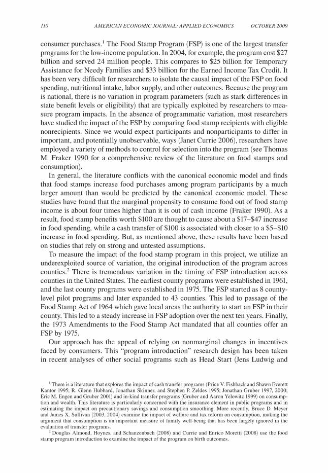
consumer purchases.1 The Food Stamp Program (FSP) is one of the largest transfer programs for the low-income population. In 2004, for example, the program cost $27 billion and served 24 million people. This compares to $25 billion for Temporary Assistance for Needy Families and $33 billion for the Earned Income Tax Credit. It has been very difficult for researchers to isolate the causal impact of the FSP on food spending, nutritional intake, labor supply, and other outcomes. Because the program is national, there is no variation in program parameters (such as stark differences in state benefit levels or eligibility) that are typically exploited by researchers to mea-sure program impacts. In the absence of programmatic variation, most researchers have studied the impact of the FSP by comparing food stamp recipients with eligible nonrecipients. Since we would expect participants and nonparticipants to differ in important, and potentially unobservable, ways (Janet Currie 2006), researchers have employed a variety of methods to control for selection into the program (see Thomas M. Fraker 1990 for a comprehensive review of the literature on food stamps and consumption).
In general, the literature conflicts with the canonical economic model and finds that food stamps increase food purchases among program participants by a much larger amount than would be predicted by the canonical economic model. These studies have found that the marginal propensity to consume food out of food stamp income is about four times higher than it is out of cash income (Fraker 1990). As a result, food stamp benefits worth $100 are thought to cause about a $17–$47 increase in food spending, while a cash transfer of $100 is associated with closer to a $5–$10 increase in food spending. But, as mentioned above, these results have been based on studies that rely on strong and untested assumptions.
To measure the impact of the food stamp program in this project, we utilize an underexploited source of variation, the original introduction of the program across counties.2 There is tremendous variation in the timing of FSP introduction across counties in the United States. The earliest county programs were established in 1961, and the last county programs were established in 1975. The FSP started as 8 county-level pilot programs and later expanded to 43 counties. This led to passage of the Food Stamp Act of 1964 which gave local areas the authority to start an FSP in their county. This led to a steady increase in FSP adoption over the next ten years. Finally, the 1973 Amendments to the Food Stamp Act mandated that all counties offer an FSP by 1975.
Our approach has the appeal of relying on nonmarginal changes in incentives faced by consumers. This “program introduction” research design has been taken in recent analyses of other social programs such as Head Start (Jens Ludwig and
1 There is a literature that explores the impact of cash transfer programs (Price V. Fishback and Shawn Everett Kantor 1995; R. Glenn Hubbard, Jonathan Skinner, and Stephen P. Zeldes 1995; Jonathan Gruber 1997, 2000; Eric M. Engen and Gruber 2001) and in-kind transfer programs (Gruber and Aaron Yelowitz 1999) on consump-tion and wealth. This literature is particularly concerned with the insurance element in public programs and in estimating the impact on precautionary savings and consumption smoothing. More recently, Bruce D. Meyer and James X. Sullivan (2003, 2004) examine the impact of welfare and tax reform on consumption, making the argument that consumption is an important measure of family well-being that has been largely ignored in the evaluation of transfer programs.
2 Douglas Almond, Hoynes, and Schanzenbach (2008) and Currie and Enrico Moretti (2008) use the food stamp program introduction to examine the impact of the program on birth outcomes.

VoL. 1 no. 4 111HoYnES AnD SCHAnZEnBACH: rESPonSES To in-KinD TrAnSFErS
Douglas Miller 2007), Medicare (Amy Finkelstein and Robin McKnight 2008), and Title I (Elizabeth U. Cascio et al. forthcoming). It is also part of a larger literature examining the impact of the Great Society and Civil Rights era (for example, see Almond, Kenneth Y. Chay, and Michael Greenstone 2006).
We use data from the Panel Study of Income Dynamics (PSID) from 1968–1978 to examine the impact of the FSP on food consumption.3 Specifically, we look at expenditures on food spent at home, meals out, and total food spending. We test theoretical predictions that food stamps lead to a decrease in out of pocket spending on food and an increase in total food spending. Further, we examine whether con-sumers are inframarginal—that is a dollar in cash income and a dollar in food stamp benefits generate equal impacts on food spending.
We employ a difference-in-difference model, where the treatment is at the county level, with controls for county and year fixed effects and state linear time trends. In this model, identification requires that there are no contemporaneous county level trends that are correlated with food stamp introduction and family economic out-comes. We also estimate a triple difference model that uses variation across sub-groups with varying propensities for being affected by food stamps.
We control for possible confounders in two ways. First, we examine the determi-nants of the FSP introduction, and find that earlier food stamp program introduction occurs in counties that are more populous, urban, black, low income, and with a smaller fraction of land used in agriculture. While these county characteristics are statistically significant determinants of county FSP implementation, we find that they explain little of the overall variation in food stamp implementation. Nonetheless, we include linear trends interacted with these pretreatment variables to control for possible (observable, parametric) trends across counties. Second, FSP introduction took place during a period of great expansion in programs for the poor in the United States. To control for the possible coincident expansion of other programs such as Aid to Families with Dependent Children (AFDC), Medicaid, Medicare, and Social Security, we include county-by-year controls for federal spending on other social programs. We show that the results are very robust to adding these controls, sug-gesting that our identification is “clean.” Finally, we estimate event study models that further support the validity of the research design.
Overall, our results indicate that people behave as the theory predicts. We find that the introduction of FSP leads to a decrease in out-of-pocket food spending and an increase in overall food expenditures. The expected effect on the propensity to eat meals out at restaurants is theoretically indeterminate, and we find mixed and statis-tically insignificant results. The results are precisely estimated for total food spend-ing, with less precision in estimating the impacts on out-of-pocket food costs and meals out. Further, we find evidence that the marginal propensity to consume food out of food stamp income is close to the marginal propensity to consume out of cash income. In addition, those predicted to be constrained (at the kink in the food/non-food budget set) experience larger increases in food spending with the introduction of food stamps. The results are robust to many sensitivity tests including adding
3 Because the PSID begins in 1968, we can only take advantage of the counties that adopt food stamp pro-grams after that time.

112 AmEriCAn EConomiC JournAL: APPLiED EConomiCS oCToBEr 2009
more fixed effects, examining subgroups of the sample, and placebo tests on groups not likely to use food stamps.
The remainder of the paper proceeds as follows. Section I presents a history of the food stamp program. Section II discusses the expected effects of the program, and Section III reviews the existing literature. Section IV describes the data, and Section V presents the methodology. Section VI presents our results, and Section VII concludes.
I. Introduction of Food Stamp Program
The origins of the modern Food Stamp Program began in 1961 with President John F. Kennedy’s first executive order establishing eight county-level pilot pro-grams.4 The pilot programs were later expanded to 43 counties in 1962 and 1963. The success of these pilot programs led to the Food Stamp Act of 1964 (FSA). The FSA gave local areas the authority to start up an FSP in their county. As with the current FSP, the program was federally funded and benefit levels did not vary across areas. In the period following the passage of the FSA, there was a steady stream of counties initiating food stamp programs. Support for requiring food stamp programs grew due to a national spotlight on hunger (Jeffrey M. Berry 1984). This interest culminated in the passage of the 1973 Amendments to the Food Stamp Act, which mandated that all counties offer an FSP by 1975.
At the time the FSP was introduced and expanded, hunger and nutritional deficien-cies were not uncommon among Americans. For example, a survey of low-income families in Texas, Louisiana, Kentucky, and West Virginia in the period 1968–1970 found that 15 percent of whites and 37 percent of blacks had low hemoglobin levels (Peter K. Eisinger 1998). There were also relatively high rates of deficiencies in vitamin C, riboflavin, and protein. A 1968 CBS documentary, “Hunger in America,” raised national awareness of the problem and possibly influenced the policy debate on the FSP (Berry 1984).
It is important to understand the political context in which the FSP was intro-duced in the United States. Prior to the modern day FSP, some counties provided food aid through the commodity distribution program (CDP). The main goal of the CDP was to support farm prices and farm income by removing surplus commodi-ties from the market. It was seen, however, as inadequate to promote the nutritional well-being of low-income persons, and the Citizens’ Board of Inquiry into Hunger and Malnutrition in the United States declared that “the commodity distribution pro-gram is a failure” in its 1968 report Hunger, uSA (Citizen’s Board of Inquiry 1968). Of the 1,000 poorest counties, one-third offered no food assistance of any kind in 1967. Furthermore, in counties that did offer the program, the commodities rarely reached a majority of the poor population because of obstacles such as distribution centers that were difficult to reach, the limited range of products, and infrequent timing of the distribution of goods. Consequently, debate about moving from the CDP to the FSP pitted powerful agricultural interests against advocates for the poor
4 This section is based on Berry (1984) and Maurice MacDonald (1977).

VoL. 1 no. 4 113HoYnES AnD SCHAnZEnBACH: rESPonSES To in-KinD TrAnSFErS
(MacDonald 1977; Berry 1984). In fact, as described in Berry (1984), passage of the 1964 Food Stamp Act was achieved through classic legislative logrolling. The farm interest coalition (Southern Democrats, Republicans) wanted to pass an impor-tant cotton-wheat subsidy bill, while advocates for the poor (Northern Democrats) wanted to pass the FSA. Neither had majorities, yet they combined forces, supported each others bills, and both bills passed.
This political history is important because it illustrates that there was significant heterogeneity across the country in support for the FSP. Remember that the 1964 Act allowed for counties to voluntarily set up food stamp programs. The above discus-sion suggests that counties with strong support for farming interests may adopt the FSP later in the period while those with strong support for the low-income popula-tion may adopt the FSP earlier in the period. Consequently, the food stamp program introduction may not be completely exogenous. We return to this below.
Figure 1 summarizes the overall pattern of FSP introduction. In particular, the figure plots the percent of counties offering the FSP, where the counties are weighted by their 1970 population. Note that this is not the food stamp caseload, but represents the percent of the national population that lived in an area offering an FSP. The figure shows that there was a long ramp-up period between 1964 and 1975, leading to the eventual universal coverage of the FSP. For example in 1968 (when the PSID begins) about half of the population lived in counties with an FSP and by 1972 this rose to over 80 percent. It is this ramp-up period that forms the basis of our research design.5
It is important to understand the CDP in order to interpret the magnitude of the FSP effects. For example, if all food stamp recipients had previously received an equal amount of commodities, we would not expect to find any impact of the FSP on consumption. On the other hand, if counties adopting the FSP did not previously have access to the CDP or if the FSP provided a “larger” or “better” set of consump-tion choices, then the estimated coefficients would pick up the effect of the introduc-tion of the program.
The evidence shows that the FSP represents an important “treatment” over and above the CDP. First, as shown in Figure 2, the FSP caseload quickly overtakes the CDP caseload. In fact, the CDP was far from universally available prior to the FSP. For example, in 1967, 35 percent of counties (not population-weighted) offered nei-ther an FSP nor a CDP, 38 percent of counties offered only a CDP, 21 percent offered only an FSP, and 6 percent of counties offered both a CDP and an FSP. Second, the CDP provided a very narrow set of commodities. The most frequently available commodities were flour, cornmeal, rice, dried milk, peanut butter, and rolled wheat (Citizens’ Board of Inquiry 1968). In contrast, the food stamp benefits can be used to purchase all food items (except hot foods for immediate consumption, alcoholic beverages, and vitamins). Further, the commodities were distributed infrequently. Finally, analyses of food intake in counties converting from a CDP to an FSP found that in its allowing participants to purchase a wide variety of food, including fresh meat and vegetables, the FSP represented an important increase in the quality and
5 County FSP implementation dates are reported in USDA annual reports on county food stamp caseloads (US Department of Agriculture, various years).

114 AmEriCAn EConomiC JournAL: APPLiED EConomiCS oCToBEr 2009
0
20
40
60
80
100
1960 1962 1964 1966 1968 1970 1972 1974
Cou
ntie
s pa
rtic
ipat
ing
in F
SP
(w
eigh
ted
perc
ent) 1961: Pilot
programs
inititated
1964 FSA:
counties can
start FSP
1973 Amend:
mandatory FSP by
1975
1968: PSID
begins
Figure 1. Cumulative Percent of Counties with Food Stamp Program, 1960–1975
Source: Authors’ tabulations of county FSP start dates. Counties are weighted by their 1960 population.
0
4
8
12
16
20
1969 1970 1971 1972 1973 1974 1975 1976
Year
Mon
thly
ave
rage
par
ticip
atio
n (m
illio
ns)
Food stamp program Commodity distribution program
Figure 2. Food Assistance Program Participation, 1968–1976
Source: Author created figure based on a table from the book Feeding Hungry People: rulemaking in the Food Stamp Program (Berry 1984).

Vol. 1 No. 4 115HoYNES AND SCHANZENBACH: RESPoNSES To IN-KIND TRANSFERS
quantity of food in comparison to the CDP (US Congressional Budget Office 1977, Currie and Moretti 2008).6
To get more insight into the geographic variation in the ramp-up to a univer-sal FSP, Figure 3 shows the timing of food stamp introduction by county. In the figure, the shading of the counties is assigned by county FSP startup date, with darker shading denoting a later startup date. This shows a great deal of variation in FSP introduction within and across states. Our basic identification strategy uses this county-level variation in food stamp “treatment.”
To further explore the degree of within-state variation in FSP start dates, Figure 4 presents FSP coverage rates for selected states for 1961–1975.7 This figure, as in Figure 1, plots the percent of the population (in this case, in the state) that lives in a county offering food stamps. In some states, such as Massachusetts and Florida, there was little or no within-state variation in food stamp start dates. In other states, such as California and North Carolina, the ramp-up was gradual within state. In most states, the county-level food stamp introduction took place in a narrower period than for the country as a whole.
As discussed above, the 1964 FSA allowed counties to start an FSP—but it was voluntary. Therefore, the validity of our research design requires exogeneity of the county FSP start dates. The previous discussion suggests that northern, urban counties, with large poor populations, were more likely to adopt food stamp pro-grams earlier while southern, rural counties, with strong agricultural interests, adopted food stamp later. This systematic variation in food stamp adoption could
6 Theoretically, counties were not supposed to have both an FSP and a CDP in place at the same time, but, in practice, some places did offer both. We have not been able to find a consistent time series for county participation in the CDP. Consequently, we are unable to use this information in our empirical analysis.
7 Similar figures for the full panel of states are available on the Web as Appendix Figures 1a and 1b.
Figure 3. Food Stamp Program Start Date, by County (1961–1975)
Source: Authors’ tabulations of food stamp administrative data (US Department of Agriculture, various years).
1961–1966
1967–1968
1969–1971
1972–1973
1974–1976

116 AmEriCAn EConomiC JournAL: APPLiED EConomiCS oCToBEr 2009
lead to spurious estimates of the programs’ impact if those same county characteris-tics are associated with differential trends in the outcome variables.
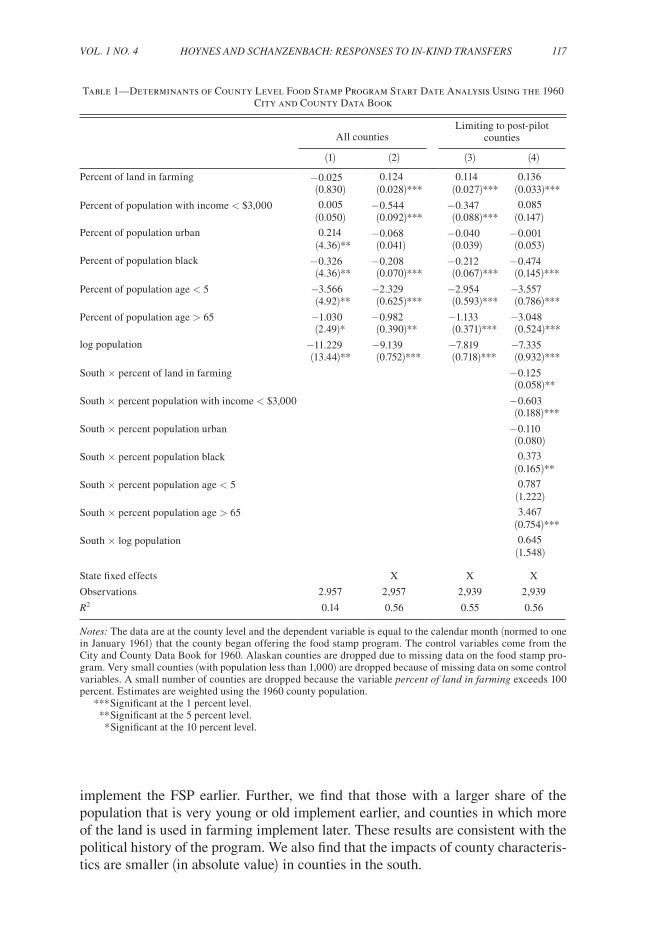
To explore this, we compiled characteristics of counties in 1960, on the eve of the first food stamp pilot programs. We use these “pre” characteristics to predict the date that the county adopted a food stamp program. The dependent variable is the month and year of the county’s food stamp start date, expressed as an index equal to one, beginning in January 1961. The independent variables include the percent of the 1960 population that lives in an urban area, is black, is less than 5 years of age, is 65 years old or older, has income less than $3,000 (in 1959 dollars), the percent of land in the county that is farmland, and log of the county population (constructed from the 1960 Census of Population and Census of Agriculture). We include the population to capture the fact that large counties might find the application process less costly relative to the benefits of application. All regressions are weighted by the 1960 county population.8
The results, presented in Table 1, include models with and without state fixed effects and with and without the early pilot counties (which were clearly nonran-dom). We find that counties that are more populous, urban, black, and low income
8 In this analysis, and in the subsequent analyses of the PSID, we drop observations from Alaska due to incon-sistencies in county definitions across samples and over time. Here, we also drop the (few) counties in which the percent of land used in farming was greater than 100 percent, and we drop very small counties (with population less than 1,000) because of missing data.
0
50
100
0
50
100
0
50
100
0
50
100
61 63 65 67 69 71 73 75 61 63 65 67 69 71 73 75
61 63 65 67 69 71 73 75 61 63 65 67 69 71 73 75
CA FL
MA NC
Wei
ghte
d pe
rcen
t of c
ount
ies
in s
tate
with
FS
P
Years 1961–1975
Figure 4. Trends in Weighted Percent of Counties with an FSP, Selected States
Source: Authors’ tabulations of food stamp administrative data (US Department of Agriculture, various years). Counties weighted by 1960 population.
VoL. 1 no. 4 117HoYnES AnD SCHAnZEnBACH: rESPonSES To in-KinD TrAnSFErS
implement the FSP earlier. Further, we find that those with a larger share of the population that is very young or old implement earlier, and counties in which more of the land is used in farming implement later. These results are consistent with the political history of the program. We also find that the impacts of county characteris-tics are smaller (in absolute value) in counties in the south.
Table 1—Determinants of County Level Food Stamp Program Start Date Analysis Using the 1960 City and County Data Book
All countiesLimiting to post-pilot
counties
(1) (2) (3) (4)
Percent of land in farming −0.025 0.124 0.114 0.136(0.830) (0.028)*** (0.027)*** (0.033)***
Percent of population with income < $3,000 0.005 −0.544 −0.347 0.085(0.050) (0.092)*** (0.088)*** (0.147)
Percent of population urban 0.214 −0.068 −0.040 −0.001(4.36)** (0.041) (0.039) (0.053)
Percent of population black −0.326 −0.208 −0.212 −0.474(4.36)** (0.070)*** (0.067)*** (0.145)***
Percent of population age < 5 −3.566 −2.329 −2.954 −3.557(4.92)** (0.625)*** (0.593)*** (0.786)***
Percent of population age > 65 −1.030 −0.982 −1.133 −3.048(2.49)* (0.390)** (0.371)*** (0.524)***
log population −11.229 −9.139 −7.819 −7.335(13.44)** (0.752)*** (0.718)*** (0.932)***
South × percent of land in farming −0.125(0.058)**
South × percent population with income < $3,000 −0.603(0.188)***
South × percent population urban −0.110(0.080)
South × percent population black 0.373(0.165)**
South × percent population age < 5 0.787(1.222)
South × percent population age > 65 3.467(0.754)***
South × log population 0.645(1.548)
State fixed effects X X X
Observations 2.957 2,957 2,939 2,939
r2 0.14 0.56 0.55 0.56
notes: The data are at the county level and the dependent variable is equal to the calendar month (normed to one in January 1961) that the county began offering the food stamp program. The control variables come from the City and County Data Book for 1960. Alaskan counties are dropped due to missing data on the food stamp pro-gram. Very small counties (with population less than 1,000) are dropped because of missing data on some control variables. A small number of counties are dropped because the variable percent of land in farming exceeds 100 percent. Estimates are weighted using the 1960 county population.
*** Significant at the 1 percent level. ** Significant at the 5 percent level. * Significant at the 10 percent level.

118 AmEriCAn EConomiC JournAL: APPLiED EConomiCS oCToBEr 2009
While these regression results show statistically significant impacts of the county characteristics on the timing of food stamp implementation, the quantitative impor-tance of these predictors is small and most of the variation remains unexplained.9 This is consistent with the characterization of funding limits controlling the move-ment of counties off the waiting list to start up their FSP. “The program was quite in demand, as congressmen wanted to reap the good will and publicity that accompa-nied the opening of a new project. At this time there was always a long waiting list of counties that wanted to join the program. Only funding controlled the growth of the program as it expanded” (Berry 1984, 36–37).
We view the weakness of the fit of the model as a strength when it comes to our identification approach, in that much of the variation in the implementation of FSP appears to be idiosyncratic. We should note that this only speaks to the lack of pre-dictive power of observables. Unobservables may still be a concern. Nonetheless, in order to control for possible differences in trends across counties that are spuri-ously correlated with the county treatment effect, we include interactions of these 1960 pre-treatment county characteristics with time trends in all of our models (as in Daron Acemoglu, David H. Autor, and David Lyle 2004).10 The results are little impacted by the inclusion of these trends.
This period of FSP introduction took place as part of the much larger federal “war on poverty.” For example, this period included the introduction of Medicaid; Medicare; Head Start; and the Supplemental Nutrition Program for Women, Infants and Children (WIC). Further, AFDC, Social Security, and disability income pro-grams expanded. If these programs are mainly varying at the state level, then our controls for state linear time trends or state-year fixed effects should absorb these program impacts. However, to control for the possible coincident expansion of other programs, we also include annual measures of county per capita transfer payments for cash income support, medical care, and retirement and disability programs.11
II. Expected Effects of Food Stamp Introduction
The current FSP provides a benefit to eligible families that is the difference between the cost of a family-size adjusted “thrifty food plan” (e.g., the guarantee in transfer program parlance) and the amount a family can afford to spend on food. In this scenario, as understood in the canonical Herman M. Southworth (1945) model, and illustrated in Figure 5, the original budget line reflects the trade-off between food and all other goods, and is shifted out horizontally by the amount of food stamps received (labeled here as BF). The basic prediction of this transfer is that overall spending on food and other goods will increase as shown by the illustrated
9 To illustrate this, Web Appendix Figure 2 provides scatter plots of county characteristics (x-axis) against the county FSP implementation date (y-axis). This figure shows that the magnitude of the association between the county characteristics and the food stamp start date is weak, and there is an enormous amount of variation that is not explained by the characteristics.
10 Another approach might be to use these estimates to form propensity scores for matching counties. However, the weak fit of the model renders this less appealing.
11 We have no documentation that any of these programs had the county roll out feature that provides the basis for our identification of the FSP. With respect to other nutrition programs, the National School Lunch Program had long been established, having started in 1946, and WIC was implemented more universally in 1972.

VoL. 1 no. 4 119HoYnES AnD SCHAnZEnBACH: rESPonSES To in-KinD TrAnSFErS
optimal points A 0* and A1
*. Out-of-pocket food expenses are expected to decrease (here, the change is F2−F0). Consequently, the increase in total food consumption, shown here as F1−F0, is less than the increase in food stamps BF . It is possible that a household with high demand for nonfood relative to food might be constrained by the in-kind nature of food stamps (relative to a cash transfer) and would locate at the kink, as in point B1
*. For these families, food stamps would lead to a larger increase in food consumption than an equivalent transfer in cash.12
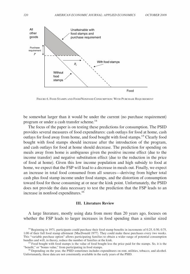
Prior to 1979 (and during the time period studied here), families had to make an up-front cash payment to receive the food stamp benefits. This feature, called the “purchase requirement,” did not change the magnitude of the benefits a family received.13 Figure 6 shows the budget constraint in this case, where the amount of the purchase requirement is P. Note that the sloped part of the budget constraint is still shifted outward by the food stamp benefit (again BF), but the top is censored, and the attainable budget set is smaller. That is, a participant can no longer choose any con-sumption bundles that would have them spending more than their total income (Y ) minus P. As a result, there may be more people consuming at the kink in the budget constraint under the purchase requirement program than under the current program. This suggests that in our analysis, the impact of food stamps on food spending may
12 Implicit in Figure 5 is the assumption that relative prices of food to nonfood are unchanged with the FSP. While it seems possible that the FSP could have led to increases in food prices (through increases in demand among the low-income population), we have no data to test this hypothesis.
13 That is, if the family was deemed able to afford to spend $60 on food, but the cost of the thrifty food plan was $80, the family could purchase $80 in food stamps for the cash price of $60. Under today’s program, a similar family would receive $20 in food stamps and would not have to outlay any cash.
All other goods
Region unattainablewith food stamps
With food stamps[voucher B
F ]
B1*
B0*
A1*
A0*
FoodF2
F0
F1
BF
Figure 5. Food Stamps and Food/Nonfood Consumption: No Purchase Requirement
120 AmEriCAn EConomiC JournAL: APPLiED EConomiCS oCToBEr 2009
be somewhat larger than it would be under the current (no purchase requirement) program or under a cash transfer scheme.14
The focus of the paper is on testing these predictions for consumption. The PSID provides several measures of food expenditures: cash outlays for food at home, cash outlays for food away from home, and food bought with food stamps.15 Clearly food bought with food stamps should increase after the introduction of the program, and cash outlays for food at home should decrease. The prediction for spending on meals away from home is ambiguous given the positive income effect (due to the income transfer) and negative substitution effect (due to the reduction in the price of food at home). Given this low income population and high subsidy to food at home, we expect that the FSP will lead to a decrease in meals out. Finally, we expect an increase in total food consumed from all sources—deriving from higher total cash plus food stamp income under food stamps, and the distortion of consumption toward food for those consuming at or near the kink point. Unfortunately, the PSID does not provide the data necessary to test the prediction that the FSP leads to an increase in nonfood expenditures.16
III. Literature Review
A large literature, mostly using data from more than 20 years ago, focuses on whether the FSP leads to larger increases in food spending than a similar sized
14 Beginning in 1971, participants could purchase their food stamp benefits in increments of 0.25, 0.50, 0.75, 1.00 of their full food stamp allotment (MacDonald 1977). They could make these purchases every two weeks. This “variable purchase option” allows participating families to obtain a wider range of potential consumption bundles and will, in theory, reduce the number of families at the kink.
15 Food bought with food stamps is the value of food bought less the price paid for the stamps. So, it is the “benefit,” or “bonus value,” from participating in food stamps.
16 Depending on the year, the PSID sometimes includes expenditures on rent, utilities, tobacco, and alcohol. Unfortunately, these data are not consistently available in the early years of the PSID.
With food stamps
Food
BF
All other goods
Unattainable with food stamps andpurchase requirement
Purchaserequirement
P
Withoutfood stamps
B0*
Figure 6: Food Stamps and Food/Nonfood Consumption: With Purchase Requirement
Figure 6. Food Stamps and Food/Nonfood Consumption: With Purchase Requirement

VoL. 1 no. 4 121HoYnES AnD SCHAnZEnBACH: rESPonSES To in-KinD TrAnSFErS
cash transfer. The observational studies (summarized in Fraker 1990 and J. William Levedahl 1995) typically estimate the marginal propensity to consume food using the following linear specification (or semi-log or double-log specification):
(1) fspendi = β0 + β1cashi 1 β2 fstampi 1 Zi γ 1 εi,
where fspendi is expenditure on food for household i; cashi and fstampi are income in cash and from food stamps, respectively; Zi is a vector of covariates such as house-hold size and age/gender makeup; and εi is a disturbance term. Here, the primary impact of food stamps is measured as the increased consumption out of food stamps compared to cash income, as measured by the differences in estimated coefficients by income type in equation (1).
This literature suffers from many of the standard shortcomings of observational studies conducted in the 1970s and 1980s. Importantly, food stamp participation is taken as exogenous, and the estimates are identified by comparing food stamp recip-ients and “similar” nonrecipients. (Again, the program is a national one, so there is no scope to use variation in eligibility and benefits across states.) Standard models of program participation (Currie 2006; Robert Moffitt 1983) show that program par-ticipation is a choice variable and, in this case, positively correlated with tastes for food consumption. Critically, then, these naïve comparisons between participants and nonparticipants will overstate the impact of the program.17
This upward bias seems evident in the literature. Fraker (1990), in his summary of the literature, reports that the estimates of the marginal propensity to consume (MPC) food out of food stamps are two to ten times higher than the estimated MPC food out of cash income. The median study in Fraker’s literature review reports a marginal propensity to consume food out of food stamp income that is 3.8 times as large as that from cash income.18 These findings are often interpreted as evidence that food stamps increase food spending by more than an equivalent cash-trans-fer system. Our research design takes this early literature to task and identifies the effects by variation in the timing of food stamp introduction across areas rather than the comparison of recipients and nonrecipients.
Because the previous literature soundly supports the idea that the MPC out of food stamps is larger than it is out of cash, the USDA conducted a handful of ran-domized experiments in the early 1990s in which the treatment group received its food stamp benefits in cash. The results of these experiments indicate that spending on food was about 5 percent higher among the group that received benefits paid in stamps (Fraker et al. 1992; James C. Ohls et al. 1992). Schanzenbach (2007) finds that the mean treatment effect is a combination of no difference in food spending
17 Other studies compare food stamp recipients to higher income families who are not eligible for food stamps. These studies rely heavily on the functional form imposed on income, which may fail to adequately account for the Engel curve, which predicts that spending on food accounts for a larger share of total spending at very low levels of income. If the nonlinearities in food spending implied by the Engel curve coincide with income from food stamps, then the estimated coefficient on food stamp income could be biased (Diane Whitmore 2002).
18 The MPC out of cash is estimated to be 0.03–0.17 (with most estimates between 0.05 and 0.10), and the MPC out of food stamps is estimated to be 0.17–0.47.

122 AmEriCAn EConomiC JournAL: APPLiED EConomiCS oCToBEr 2009
among inframarginal recipients, and a substantial shift in consumption toward food for stamp recipients who are constrained. Note, though, that the experimental lit-erature asks a slightly different question than we do in this paper. The experimen-tal literature measures the impact on spending of replacing food stamps with cash while holding total income constant. In this paper, we measure the impact on spend-ing of the introduction of the FSP, which significantly increased total income for recipients.
IV. Data
The PSID is a panel dataset that began in 1968 with a sample of about 5,000 households, and subsequently all members (and descendants) of these original sur-vey families are re-interviewed annually. The original 1968 sample consists of two subsamples: a nationally representative subsample of 3,000 households, and a sub-sample of 1,900 households selected from an existing sample of low-income and minority populations. To adjust for this nonrandom composition, the PSID includes weights designed to eliminate biases attributable to the oversampling of low-income groups and to attrition. All results use the weights provided by the PSID.
Beyond the labor market and demographic variables that are the focus of the PSID, the survey includes annual food expenditures for food consumed at home, away from home, and food purchased with food stamps (the value of food purchased less the purchase requirement). These data have been used by many researchers examining impacts of social programs on consumption (for example, see Richard Blundell and Luigi Pistaferri 2003; Gruber 1997, 2000; and Hubbard, Skinner, and Zeldes 1995). The public-use release of the PSID includes state identifiers. Through special arrangement, we have obtained county identifiers for each family in each year.
We use data from interview years 1968 to 1978. We stop the sample in 1978 so that our entire analysis period is before the end of the purchase requirement (which occurred in 1979). Our sample excludes 1973 because the food consumption variables were not included in that survey, and 1968 because of inconsistencies in the definition of the food variables in that survey.19 We also exclude observations from Alaska (because of difficulties in matching counties with FSP provision areas), and we trim the sample of a few outliers (observations in which the ratio of food spending to income exceeds 0.85, in which total annual food expenditures were less than $100 in 2005 dollars, or in which annual family income was less than $500 in 2005 dollars). A test of sensitivity to these trimmed observations is included in Web Appendix Table 3.
There is some ambiguity in what time frame the food variables correspond to. The survey is taken in spring and families are asked about “typical food consumption.”20
19 In 1968, “food assistance” (rather than food stamp benefits) is provided that includes commodity distribu-tion program, food stamp program, and other in-kind benefits. Further, the cost of meals away from home is defined more broadly than in later years and the amounts are bracketed.
20 Specifically, spending on food at home and food out were first asked about “weekly” (1968–1969), then for “last year” (1970–1976), then finally settled into “annual spending” starting in 1976. Between 1968 and 1974, respondents were asked to report food stamp receipt “last year,” but it is thought that most respondents answered

VoL. 1 no. 4 123HoYnES AnD SCHAnZEnBACH: rESPonSES To in-KinD TrAnSFErS
The PSID then annualizes this measure and applies it to the prior calendar year. Nonetheless, we assume, as other researchers have, that the food spending vari-ables apply to this year (Blundell and Pistaferi 2003; Gruber 1997, 2000; Hubbard, Skinner, and Zeldes 1995; Zeldes 1989).
Unlike virtually all other US public assistance programs, there is no categorical eligibility for the food stamp program. That is, eligibility depends on income and asset tests, but it is not targeted to particular demographic groups, such as single parents with children. Table 2 presents food stamp participation rates by education, family type, and race, based on the 1976–1978 PSID (chosen to be after all counties have adopted the program and before the elimination of the purchase requirement). These tabulations show that while food stamp participation is highest among single parent families with children, the participation is widespread across many demo-graphic groups. For example, among families where the head of household has less than 12 years of education, 46 percent of single parent families with children, 14 percent of married couples with children, 14 percent of single nonelderly persons
about their current status. As a result, starting in 1975, the question was changed to inquire about food stamp receipt “last month.”
Table 2—Food Stamp Participation Rates by Demographic Group
Education group
All
Less thanhigh school
High school grad
More thanhigh school
Panel A. All races
All family types 0.08 0.14 0.06 0.02Single with children 0.32 0.46 0.23 0.15Married with children 0.07 0.14 0.06 0.01Single, no children 0.07 0.14 0.05 0.03Married, no children 0.02 0.04 0.01 0.01Single, no children, elderly 0.07 0.10 0.03 0.01Married, no children, elderly 0.03 0.05 0.00 0.00
Panel B. White
All family types 0.05 0.10 0.04 0.02Single with children 0.22 0.38 0.14 0.07Married with children 0.05 0.12 0.05 0.01Single, no children 0.05 0.11 0.04 0.03Married, no children 0.01 0.03 0.00 0.01Single, no children, elderly 0.05 0.07 0.02 0.01Married, no children, elderly 0.02 0.04 0.00 0.00
Panel C. nonwhite
All family types 0.22 0.28 0.18 0.09Single with children 0.51 0.56 0.44 0.43Married with children 0.16 0.22 0.14 0.03Single, no children 0.13 0.20 0.09 0.04Married, no children 0.06 0.10 0.02 0.02Single, no children, elderly 0.24 0.25 0.11 0.00Married, no children, elderly 0.10 0.13 0.00 0.00
notes: Weighted means of food stamp participation rates using families in the 1976–1978 Panel Study of Income Dynamics. These years were chosen because, by 1976, all counties had implemented food stamp programs, yet, it was before the elimination of the purchase requirement in 1979.

124 AmEriCAn EConomiC JournAL: APPLiED EConomiCS oCToBEr 2009
with no children, and 10 percent of single elderly persons participate in food stamps. The rates are uniformly higher among black families, with 56 percent of single nonelderly parent families with children (where the head of household has less than 12 years of education) participating in food stamps.21
We start by measuring the impact of FSP introduction on the sample of all nonelderly families (e.g., head of household is less than 65 years old), then restrict the subsamples of the data limited to groups with a higher probability of being affected by food stamps (nonelderly singles and families headed by a person with 12 or fewer years of education, female-headed households).22
Our final samples include 39,623 (family-year) observations for all nonelderly households, 30,905 observations for nonelderly low-education households, and 6,002 observations for female-headed households. Web Appendix Table 1 presents some basic descriptive statistics for these samples. All dollar amounts are in 2005 dollars and real variables are constructed using separate CPIs for food at home and food away from home. For the nonelderly, low-education sample, annual food spending (in 2005 dollars) averages $7,914 overall and $7,280 among food stamp recipient families. Food spending is, on average, 19.6 percent of income overall and 36 percent among food stamp recipients. Among food stamp recipients, food stamp benefits average 33 per-cent of total food spending, suggesting that the typical family is not constrained. In fact, further tabulations show that only 5 percent of food stamp recipients are observed to be constrained (have total food consumption ≤ food stamp benefits).
Using county identifiers, we merge the PSID with the FSP policy variables (US Department of Agriculture, various years), 1960 county characteristics (US Department of Commerce 1978), and annual per capita county transfers from the, Regional Economic Information System (REIS) (US Department of Commerce 2007). The REIS captures all federal transfers to countries that we use to construct three per capita county transfer variables: cash public assistance benefits (AFDC, Supplemental Security Income (SSI), and General Assistance), medical spending (Medicare and Military health care), and cash retirement and disability payments.
V. Methodology
We estimate a difference-in-difference model based on the PSID spanning the period during which the FSP is introduced. In particular, we estimate the following model:
(2) yict = α + δFSPct + Xit β + γ1Zc 60 t + γ2TPct + ηc + δt + λs t + εict,
where yict is the outcome variable (such as the log of total food spending) for family i living in county c in year t. FSPct is an indicator variable equal to one if county c in year t has an FSP program. Xit are family characteristics. Zc 60 are 1960 county
21 The participation rates are very similar when tabulated on the larger sample sizes of the Current Population Survey in 1980 (the first year in which food stamp information is available).
22 We limit the analysis to the nonelderly because of low take-up rates among the elderly (Currie 2003; Steven J. Haider, Alison Jacknowitz, and Robert F. Schoeni 2003). The results are qualitatively unchanged when we include the elderly.

VoL. 1 no. 4 125HoYnES AnD SCHAnZEnBACH: rESPonSES To in-KinD TrAnSFErS
characteristics.23 TPct are the REIS per capita county transfer income variables, ηc are county fixed effects, δt are year effects, and λst are state-specific linear time trends. We also show results with state-year fixed effects. All estimates are weighted using the PSID family weight, and the standard errors are clustered on county (Marianne Bertrand, Esther Duflo, and Sendhil Mullainathan 2004).
The controls X include education, race, urban location, state unemployment rate, and, in some specifications, the log of family cash income. As suggested by Currie (2003), X also includes a full set of fixed effects for the number of children and number of adults in the family to control nonparametrically for the differences in food needs across families.
As described above, the food variables in the PSID measure expenditures as of the time of the interview, which is fielded in spring of each year. Thus, t in equation (2) refers to the interview year. Given this timing, we set the treatment variable FSPct to one if county c has an FSP program in place by January of year t.24
VI. Results for Expenditures on Food
We begin with estimates for the full nonelderly sample and the two subsamples at higher risk to be impacted by the introduction of FSP (households with non-elderly heads with 12 or fewer years of education, and female-headed households). We consider four outcome variables: whether the household reported using any food stamps (i.e., whether there was a program), the log of cash (non food stamp) food expenditure at home, a dummy for any meals out, and the log of total (including food stamp) food expenditures. The meals out variable is equal to one if a household reports spending any money on meals out in a typical week. About 70 percent of the low-educated, nonelderly sample, and just over one-half of single-mother families, report any spending on meals out (Web Appendix Table 1). Total food expenditures includes money spent on food at home, food out, and also includes food purchased with food stamps, and the value of any other free meals or food that the household received.
These difference-in-difference results for the three samples are presented in Table 3. The estimates in panel A show that the introduction of the food stamp pro-gram leads to increases in food stamp receipt (as expected).25 The results in panels B through D show that FSP introduction leads to increases in total food spend-ing, decreases in propensity to eat out, and mixed results for cash food expendi-tures. To scale up the results to be per food stamp family (effect of the treatment on the treated), the numbers in italics divide the parameter estimates by the sample mean food stamp participation (Table 2). For female-headed households (column 3), FSP introduction leads to a large, statistically significant increase in total food
23 The variables in Z include the log of the population; the percent of land in farming; and the percent of popu-lation black, urban, age less than five, age greater than 65, and with income less than $3,000.
24 There is evidence (Berry 1984) that it took some time to ramp up the new county FSP programs. We have explored the sensitivity to lagging the treatment effects, and while the specific estimates change somewhat, the results are qualitatively similar.
25 We can interpret the coefficient as the effective participation rate. Note that these implied participation rates are somewhat lower than those implied in Table 2 and may be due to a program ramp-up period taking place.

126 AmEriCAn EConomiC JournAL: APPLiED EConomiCS oCToBEr 2009
Table 3—Impact of Food Stamp Introduction on Family Food Expenditures Difference-in-Difference Models
All nonelderly
households
Nonelderly, head education
,= 12 yearsFemale heads
(1) (2) (3)
Panel A. Any food stamps (0/1)County FSP implemented 0.035 0.050 0.194
(0.007)*** (0.009)*** (0.040)***
Observations 39,623 30,905 6,002
r2 0.22 0.25 0.40
Panel B. Log of cash (non food stamp) food expenditures at home
County FSP implemented −0.006 −0.008 0.042(0.016) (0.019) (0.055)
−0.081 −0.078 0.116
Observations 39,243 30,541 5,788
r2 0.55 0.53 0.45
Panel C. Any meals out (0/1)County FSP implemented −0.005 −0.003 −0.055
(0.015) (0.019) (0.048)−0.068 −0.029 −0.152
Observations 39,623 30,905 6,002
r2 0.26 0.25 0.38
Panel D. Log of total (including food stamp) food expenditures
County FSP implemented 0.007 0.016 0.102(0.013) (0.016) (0.042)**0.095 0.157 0.282
Observations 39,623 30,905 6,002
r2 0.52 0.51 0.49
Demographics X X X
1960 cty vars × linear time X X X
Year and county fixed effects X X X
Per capita cty transfers X X X
State × linear time X X X
notes: Each parameter is from a separate regression of the outcome variable on a dummy variable equal to one if the county-year observation had a food stamp program in place by January of that year. The samples include 1969–1972 and 1974–1978, and exclude observations from Alaska and observations with unusual expenditure values (annual food expenditures less than $100, annual family income less than $500, or income share on food greater than 0.85). For details on this sample selection, see text. Estimation samples include all nonelderly fami-lies (column 1), nonelderly families with head of household having education less than or equal to 12 years (col-umn 2), and female-headed households (column 3). All outcome variables correspond to annual measures taken as of the interview (in spring of the interview year). Demographic controls include dummies for education, num-ber of children, and number of adults, race, urban location, and state unemployment rate. County variables for 1960 include log of population, percent of land in farming, percent of population black, urban, age < 5, age > 65, and with income less than $3,000, each interacted with a linear time trend. Per capita county transfer income includes measures for public assistance (AFDC, General Assistance), medical care (Medicare, Medicaid, mil-itary), and retirement and disability benefits. Estimates are weighted using the PSID weight and clustered on county. Standard errors are in parentheses. The numbers in italics inflate the parameter estimate by the sample food stamp participation rate in 1978.
*** Significant at the 1 percent level. ** Significant at the 5 percent level. * Significant at the 10 percent level.
VoL. 1 no. 4 127HoYnES AnD SCHAnZEnBACH: rESPonSES To in-KinD TrAnSFErS
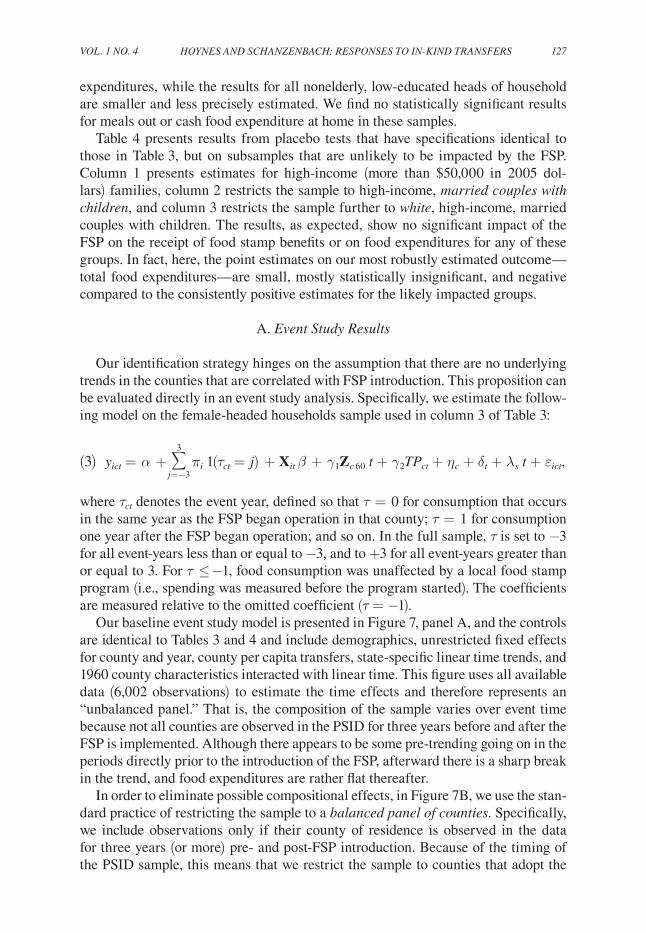
expenditures, while the results for all nonelderly, low-educated heads of household are smaller and less precisely estimated. We find no statistically significant results for meals out or cash food expenditure at home in these samples.
Table 4 presents results from placebo tests that have specifications identical to those in Table 3, but on subsamples that are unlikely to be impacted by the FSP. Column 1 presents estimates for high-income (more than $50,000 in 2005 dol-lars) families, column 2 restricts the sample to high-income, married couples with children, and column 3 restricts the sample further to white, high-income, married couples with children. The results, as expected, show no significant impact of the FSP on the receipt of food stamp benefits or on food expenditures for any of these groups. In fact, here, the point estimates on our most robustly estimated outcome—total food expenditures—are small, mostly statistically insignificant, and negative compared to the consistently positive estimates for the likely impacted groups.
A. Event Study results
Our identification strategy hinges on the assumption that there are no underlying trends in the counties that are correlated with FSP introduction. This proposition can be evaluated directly in an event study analysis. Specifically, we estimate the follow-ing model on the female-headed households sample used in column 3 of Table 3:
(3) yict = α + ∑ j=−3
3
πi 1(τct = j) + Xit β + γ1Zc 60 t + γ2TPct + ηc + δt + λs t + εict,
where τct denotes the event year, defined so that τ = 0 for consumption that occurs in the same year as the FSP began operation in that county; τ = 1 for consumption one year after the FSP began operation; and so on. In the full sample, τ is set to −3 for all event-years less than or equal to −3, and to +3 for all event-years greater than or equal to 3. For τ ≤ −1, food consumption was unaffected by a local food stamp program (i.e., spending was measured before the program started). The coefficients are measured relative to the omitted coefficient (τ = −1).
Our baseline event study model is presented in Figure 7, panel A, and the controls are identical to Tables 3 and 4 and include demographics, unrestricted fixed effects for county and year, county per capita transfers, state-specific linear time trends, and 1960 county characteristics interacted with linear time. This figure uses all available data (6,002 observations) to estimate the time effects and therefore represents an “unbalanced panel.” That is, the composition of the sample varies over event time because not all counties are observed in the PSID for three years before and after the FSP is implemented. Although there appears to be some pre-trending going on in the periods directly prior to the introduction of the FSP, afterward there is a sharp break in the trend, and food expenditures are rather flat thereafter.
In order to eliminate possible compositional effects, in Figure 7B, we use the stan-dard practice of restricting the sample to a balanced panel of counties. Specifically, we include observations only if their county of residence is observed in the data for three years (or more) pre- and post-FSP introduction. Because of the timing of the PSID sample, this means that we restrict the sample to counties that adopt the

128 AmEriCAn EConomiC JournAL: APPLiED EConomiCS oCToBEr 2009
Table 4—Impact of Food Stamp Introduction on Family Food Expenditures Difference-in-Difference Estimates on Placebo groups
All high-incomehouseholds
High-income,married
with children
White, high-income,married
with children
(1) (2) (3)Panel A. Any food stamps (0/1)County FSP implemented 0.005 0.004 0.003
(0.003) (0.004) (0.003)
Observations 16,796 9,813 1,947
r2 0.10 0.12 0.28
Panel B. Log of cash (non food stamp) food expenditures at home
County FSP implemented 0.006 −0.001 −0.036(0.015) (0.019) (0.038)
Observations 16,786 9,807 1,947
r2 0.56 0.46 0.63
Panel C. Any meals out (0/1)County FSP implemented −0.029 −0.009 −0.017
(0.018) (0.021) (0.038)
Observations 16,796 9,813 1,947
r2 0.20 0.24 0.28
Panel D. Log of total (including food stamp) food expenditures
County FSP implemented −0.004 −0.021 −0.067(0.015) (0.020) (0.038)*
Observations 16,796 9,813 1,947
r2 0.46 0.43 0.61
Demographics X X X
1960 cty vars × linear time X X X
Year and county fixed effects X X X
Per capita cty transfers X X X
State × linear time X X X
notes: Each parameter is from a separate regression of the outcome variable on a dummy variable equal to one if the county-year observation had a food stamp program in place by January of that year. The samples include 1969–1972 and 1974–1978, and exclude observations from Alaska and observations with unusual expen-diture values (annual food expenditures less than $100, annual family income less than $500, or income share on food greater than 0.85). For details on this sample selection, see text. Estimation samples include high-income (>$50,000 in 2005 dollars) families (column 1); high-income, married couples with children (column 2); and high income, white, married couples with children (column 3). All outcome variables correspond to annual measures taken as of the interview (in spring of the interview year). Demographic controls include dummies for educa-tion, number of children, and number of adults, race, urban location, and state unemployment rate. County vari-ables for 1960 include log of population, percent of land in farming, percent of population black, urban, age < 5, age > 65, and with income less than $3,000, each interacted with a linear time trend. Per capita county transfer income includes measures for public assistance (AFDC, General Assistance), medical care (Medicare, Medicaid, military), and retirement and disability benefits. Estimates are weighted using the PSID weight and clustered on county. Standard errors are in parentheses.
*** Significant at the 1 percent level. ** Significant at the 5 percent level. * Significant at the 10 percent level.

VoL. 1 no. 4 129HoYnES AnD SCHAnZEnBACH: rESPonSES To in-KinD TrAnSFErS
–0.10
–0.08
–0.06
–0.04
–0.02
0.00
0.02
0.04
0.06
0.08
0.10
Event time in years
–0.10
–0.05
0.00
0.05
0.10
0.15
0.20
0.25
0.30
0.35
–3 –2 –1 0 1 2 3
Event time in years
Include county controls
for FSP endogeneity
Exclude county controls
for policy endogeneity
Panel A. Unbalanced panel
Panel B. Balanced panel
–3 –2 –1 0 1 2 3
Figure 7. Event Study Estimates of Impact of FSP on Total (Including Food Stamp) Food Expenditures
notes: Each figure plots coefficients from an event-study analysis. Coefficients are defined as years relative to the year the Food Stamp Program is implemented in the county. Panel A includes the entire female-headed household sample, and Panel B is a balanced county sample, where observa-tions in a county are included only if there are three years pre- and post-implementation data. The specification includes controls for demographics, unrestricted fixed effects for county and year, county per capita transfers, state-specific linear time trends, and 1960 county characteristics inter-acted with linear time.

130 AmEriCAn EConomiC JournAL: APPLiED EConomiCS oCToBEr 2009
FSP after 1971. These results show strong evidence supporting the exogeneity of the FSP introduction. First, pre-trend is very flat, showing no systematic differences in county trends prior to food stamp adoption. Second, food spending increased sharply when the program was introduced. We view this as strong evidence for the validity of our identification strategy, as any confounding factor would have to very closely mimic the timing of county FSP introduction to result in a pattern like this. We also include, in Figure 7B, the results of the event study that excludes the county controls (REIS transfers TP and pre-treatment county characteristics ZC60t ). The results are nearly identical when we exclude the county trends as controls, providing further evidence of the exogeneity of the treatment.
B. Triple Difference results
In choosing our preferred sample for this analysis, we face a trade-off between sample size (using the larger sample of low-educated, nonelderly families but with overall lower participation rates) and targeting (using the smaller sample of female heads of household with higher participation rates). Here, we refine these earlier results by using the nonelderly, low-educated sample (30,905 observations), but also using a triple-difference specification that accounts for different probabilities of being affected by food stamps. In particular, we estimate the following model:
(4) yict = α + φFSPct + δFSPct Pg + Xit β + γ1Zc60 t + γ2TPct + θg
+ ηc + δt + λs t + εict .
To capture the varying risks of being treated, we multiply the FSP treatment dummy by a group-level food stamp participation rate (as in Hoyt Bleakley 2007). The group food stamp participation rate Pg comes from Table 2 and is defined for 16 groups using education (<12, 12), race (white, nonwhite), marital status (married, not mar-ried), and presence of children (yes, no).26 In addition to the controls used in Tables 3 and 4, we also include fixed effects for each group θg, and (although not shown in equation (4)) interactions of Pg with demographics, ZC60t , TP, and year fixed effects. In this triple difference model, the maintained assumption is that there are no dif-ferential trends for high participation versus low participation groups within early versus late implementing counties.
The results are presented in Table 5. In column 1, the specification is analogous to that presented in Tables 3 and 4 (includes demographics, the 1960 county charac-teristics interacted with linear time, state linear time trends, county-level per capita transfer spending, and year and county fixed effects). In column 2, we add controls for interactions between the group participation rates and the other covariates. Note, now, that the treatment effect is the interaction of FSP and the group participa-tion rate Pg, the parameter estimates represent impacts for families that take up the
26 We explored using group-level poverty rates rather than FSP participation rates, and found very similar results.

VoL. 1 no. 4 131HoYnES AnD SCHAnZEnBACH: rESPonSES To in-KinD TrAnSFErS
program (and no post-estimation scaling needs to be done, it already represents the effect of the treatment on the treated).
The first panel finds—as predicted by the theory—a small, negative impact of food stamps on cash (non food stamp) food expenditures at home. The second panel shows a small increase in the propensity to eat meals out (the theoretical prediction here is ambiguous). Both of these findings are imprecisely measured, however, and not statistically significant. In the third panel, the results show that the FSP is associated with a statistically significant and robust 19 (column 2) to 21 (column 1) percent increase in total (including food stamp) food expenditures. Overall, the results in Table 5 are consistent with the theoretical predictions, but not always statistically significantly so. The parameter estimates vary little across specifications. Finally, note that across the specifications and outcome variables, the coefficient on the main effect for FSP introduction is close to zero and never statistically significant. This is expected and encouraging because it reflects the impact of FSP introduction on a group with zero probability of being affected by food stamps (and shows the same pattern as the placebo tests in Table 4).
Interestingly, the magnitude of the results for total food expenditure from this triple difference specification is quite similar to, but much more precisely estimated than, the double difference results in Table 3. For example, the results in the first two columns of Table 5 show that FSP introduction leads to a precisely estimated 19 to 21 percent increase in total food expenditures for the nonelderly, low-education sample compared to a very imprecisely estimated 16 percent increase for the difference-in-difference estimates for the same sample in Table 3 (column 2).
C. implications for the marginal Propensity to Consume
The results in Tables 3 and 5 show that food consumption responds, as predicted, by theory. An additional test of the theory is that, if households are mostly inframa-rginal (not constrained), then an additional dollar of cash income, and an additional dollar in food stamp benefits, should lead to the same increase in food expenditures. To explore this hypothesis, we add the log of family cash income to specifications (1) and (2) in Table 5. The results are presented in columns 3 and 4. Our main models do not include a control for income because we do not have an experimentally identified estimate of income.27 Nonetheless, it is important to point out that our estimates of the impact of the FSP are little changed by the inclusion of income (columns 3 and 4).
We use these results to calculate the marginal propensity to consume (MPC) food out of cash income and food stamps. Table 6 presents the estimates and 95 percent confidence intervals of the MPC out of both types of income, and the ratio of the MPC from food stamps to the MPC from cash income.28 The top panel displays
27 We explored various instruments for family income including the BEA per capita transfer variables, but these instruments were quite weak with low predictive power.
28 The MPCs are evaluated at the mean values of food spending and income levels among food stamp recipients.

132 AmEriCAn EConomiC JournAL: APPLiED EConomiCS oCToBEr 2009
Table 5—Impact of Food Stamp Introduction on Family Food Expenditures (Triple Difference Estimates for the Nonelderly, Low-Education Sample)
Nonelderly, head education <=12 years
(1) (2) (3) (4)
Panel A. Log of cash (non food stamp) food expenditures at home
County FSP implemented × Pg −0.043 −0.073 −0.081 −0.114(0.105) (0.108) (0.101) (0.115)
County FSP implemented 0.000 0.005 0.009 0.013(0.022) (0.022) (0.021) (0.022)
Observations 30,541 30,541 30,541 30,541
r2 0.54 0.54 0.58 0.58
Panel B. Any meals out (0/1)County FSP implemented × Pg 0.101 0.109 0.079 0.084
(0.101) (0.099) (0.101) (0.099)County FSP implemented −0.014 −0.014 −0.009 −0.008
(0.022) (0.022) (0.022) (0.021)
Observations 30,905 30,905 30,905 30,905
r2 0.26 0.26 0.29 0.29
Panel C. Log of total (including food stamp) food expenditures
County FSP implemented × Pg 0.208 0.187 0.169 0.143(0.096)** (0.101)* (0.090)* (0.097)
County FSP implemented −0.005 −0.003 0.004 0.007(0.020) (0.020) (0.019) (0.020)
Observations 30,905 30,905 30,905 30,905
r2 0.52 0.52 0.58 0.58
Demographics X X X X
1960 cty vars × linear time X X X X
Per capita cty transfers X X X X
Log (real family income) X X
Group fixed effects X X X X
Year fixed effects (main and × Pg) X X X X
County fixed effects X X X X
State × linear time X X X X
Pg × other covariates (except area fixed effects) X X
notes: Each parameter is from a separate regression of the outcome variable on the Food Stamp implementation dummy multiplied by a group food stamp participation rate. The food stamp implementation dummy equals one if the county-year observation had a food stamp program in place by January of that year. The group food stamp par-ticipation rate is calculated for each education-race-marital status-presence of children cell using the 1976–1978 PSID. The sample includes 1969–1972 and 1974–1978 and excludes observations from Alaska and observations with unusual expenditure values (annual food expenditures less than $100, annual family income less than $500, or income share on food greater than 0.85). For details on this sample selection, see text. Estimation sample includes all households (singles and families) where the head is nonelderly and has a high school education or less. All outcome variables correspond to annual measures taken as of the interview (in spring of the interview year). Demographic controls include dummies for education, number of children, number of adults, race, urban location, and state unemployment rate. 1960 county variables include log of population, percent of land in farming, per-cent of population black, urban, age < 5, age > 65, and with income less than $3,000, each interacted with a linear time trend. Per capita county transfer income include measures for public assistance (AFDC, General Assistance), medical care (Medicare, Medicaid, military), and retirement and disability benefits. Estimates are weighted using the PSID weight and clustered on county. Standard errors are in parentheses.
*** Significant at the 1 percent level. ** Significant at the 5 percent level. * Significant at the 10 percent level.

VoL. 1 no. 4 133HoYnES AnD SCHAnZEnBACH: rESPonSES To in-KinD TrAnSFErS
the parameter estimates, while the bottom panel calculates the estimated marginal propensity to consume food. We present results from the low-education, nonelderly sample (using the triple difference results in Table 5), and the results for female heads of household (using the difference-in-difference results from Table 3).
The results for the nonelderly, low-education sample indicate an MPC for food out of food stamp income equal to 0.16, and an MPC for food out of cash income of 0.09. The results are consistent with the theoretical predictions—the MPC food out of food stamps is quite close to the MPC food out of cash income, suggesting that most families are inframarginal. The ratio of the point estimates of the MPCs for this sample is estimated to be 1.9. The standard errors imply that we cannot reject that the ratio is equal to one (as implied by theory), and we can reject that the ratio is four or more. This is in stark contrast to the existing literature that finds the MPC food out of food stamps to be as much as ten times larger than the MPC food out of cash income. The results for female-headed families indicate a higher MPC out of food stamps equal to 0.30 and an MPC out of cash income of 0.10, which suggests
Table 6—Estimated Marginal Propensities to Consume Food Out of Food Stamps and Cash Income
Nonelderly, head education <=12 years
Female-headed households
Table 5, column 1
(1)
Table 5, column 3
(2)
Table 3, column 3
(3)
(4)Parameter estimates
County FSP implemented 0.208 0.169 0.102 0.095(0.096)** (0.090)* (0.042)** (0.042)**
0.282 0.262
Log of real family income — 0.290 — 0.289 (0.009)*** (0.019)***
0.798
Estimated marginal propensity to consume foodMPCf out of food stamps 0.200 0.163 0.318 0.296
[0.02, 0.38] [−0.01, 0.33] [0.05, 0.58] [0.04, 0.55]
MPCf out of cash income — 0.087 — 0.098[0.08, 0.09] [0.08, 0.11]
Ratio of MPCs — 1.9 — 3.0[−0.11, 3.83] [0.33, 5.71]
Observations 30,905 30,905 6,002 6,002
notes: Each column reports results from a separate regression of the log of total food expenditures on the FSP treatment, the log of real family income (for columns 2 and 4), demographics, county variables, state-linear time, and county and year fixed effects. The results in columns 1 and 2 are from the triple-difference estimates for the nonelderly, low-education sample in Table 5 (the county FSP treatment is multiplied by Pg, the participation rate). The results in columns 3 and 4 are from the difference-in-difference estimates for female heads of household in Table 3 (numbers in italics scale up the coefficients to reflect the impact per food stamp participant family). See the notes to Tables 3 and 5 for more details. Standard errors are in parentheses. Estimates are weighted using the PSID weight and clustered on county. The marginal propensities to consume food are evaluated at mean values for food expenditures and family income among food stamp recipient families. The figures in italics in brackets are 95 percent confidence intervals around the estimated MPC.
*** Significant at the 1 percent level. ** Significant at the 5 percent level. * Significant at the 10 percent level.

134 AmEriCAn EConomiC JournAL: APPLiED EConomiCS oCToBEr 2009
that a higher proportion of these families are “constrained.” This is consistent with the Engel curve relationship, which implies that as the sample becomes more disad-vantaged, the MPC food out of cash income increases. The ratio of estimated MPCs is 3.0 among these families, but the 95 percent confidence interval both includes 1.0 and excludes ratios over 5.7 that have been found commonly in the prior literature.
It is worth pointing out that the difference between our results and the previous literature comes entirely from our lower estimate of MPC food out of food stamp income, which is the result of our credible research design. The MPC food out of cash income is not identified by our new research design and, instead, is identified cross-sectionally. We are confident, however, in the validity of this estimate for sev-eral reasons. First, the estimated MPC food out of income is unchanged when we add family fixed effects to the model (and, therefore, is identified by changes over time in income). Second, the MPC food out of income (or, equivalently, the income elasticity of food expenditures) is a widely studied and estimated parameter. Our estimates are squarely in the (quite tight) range of the estimates in a literature that uses a wide range of data (cross sectional, time series) and econometric methods. Reviews of this literature show estimates for the MPC food out of income ranging from 0.03 to 0.17 among studies focused on low-income families (Fraker 1990; Ohls and Harold Beebout 1993). Other estimates not limited to low-income populations also fall into this range (Angus S. Deaton and John Muellbauer 1980; Nicholas S. Souleles 1999; Laura Blanciforti and Richard Green 1983).
While close in magnitude (and certainly much closer than the prior literature sug-gested), our results show that the estimated MPC food out of in-kind transfers (at 0.16 for the full sample) is larger than the MPC food out of cash income at (0.09). Thus far, we have maintained that the only reason for a higher MPC food out of food stamps, compared to the MPC food out of cash income, is that households are constrained by the in-kind nature of the program (as illustrated in Figure 5). There are, however, other reasons why the MPCs may differ. The family member with control over food stamp benefits may be different from the person that controls earn-ings and other cash income. If the person with control over food stamps has greater preferences for food, then, we may find that the MPC food out of food stamps is higher than the MPC food out of cash income. Alternatively, it is possible that the in-kind transfer sets a mental target for how much a family “should” spend on food, and, as a result, alters a family’s preferences toward consuming at the budget kink point. Families may perceive that food stamp benefits are a more permanent source of income compared to earnings.
Finally, we are cautious in interpreting these “marginal” calculations (e.g., MPC) for food stamp income because of the nonmarginal nature of the research design (i.e., the design compares spending when there was no program to spending after the program was introduced, rather than a continuous measure of food stamp income).
D. Consumption Among Families Predicted to be “Constrained”
A further prediction of the theory is that families with preferences for low food consumption relative to their eligible food stamp allotment will be constrained (as in Figure 5). As a result, these families are then predicted to experience a larger

VoL. 1 no. 4 135HoYnES AnD SCHAnZEnBACH: rESPonSES To in-KinD TrAnSFErS
increase in food expenditures with food stamp introduction than other families. We explore this by creating a dummy variable equal to one if a family is predicted to be constrained (PREDCONSTR) and by interacting PREDCONSTR with the main treatment variable. We create PREDCONSTR in two steps. First, we regress food expenditures on demographics (including a rich set of dummy variables capturing the number of persons in the household by age and gender), a cubic in income, and state and year fixed effects. We use this to predict food expenditures for each fam-ily. We, then, compare the predicted food spending to the food stamps the family is eligible for, given their family income.29
The results, presented in Table 7, are consistent with theory but are estimated imprecisely. The introduction of food stamps leads to larger impacts on total food expenditures for those predicted to be constrained compared to those predicted to be inframarginal. Specifically, the coefficients on the interaction of PREDCONSTR and the treatment effect range between 0.06 and 0.07 depending on the specification, with the main treatment effect a statistically significant 0.15. Thus, constrained families increase food consumption by about 22 percent (0.07 + 0.15) compared to 15 percent among those predicted to be inframarginal and 18 percent in the full sample.
E. Sensitivity Checks
In Table 8, we explore the sensitivity of the results to specification and functional form. We present the specification tests for the triple difference models in Table 5, using the sample of low-educated, nonelderly households. (The results are qualita-tively the same for the female-headed sample.) Column 1 restates the results from column 3 in Table 5. In column 2, we include state-by-year fixed effects (instead of state linear time trends). This makes little difference in the results. The other specifi-cations in Table 8 experiment with the functional form, including food expenditures and cash income in levels (rather than logs), and a quadratic in income. To compare the results across specifications, we report MPCs out of food stamp and cash income at the bottom of the table. The results are similar across specifications, although imposing linearity on the relationship between cash income and food spending tends to reduce the MPC out of cash income.
The expansion of the FSP took place during a time of great change in the US system of government support. We address this in the main results by controlling for the county transfer variables. Another, more direct approach, is to examine the impact of the FSP on PSID reported government transfer income. In particular, with the PSID, we can measure income of the head of household and wife from AFDC, other welfare income (SSI, General Assistance), and Social Security. The results of that exercise, presented in Web Appendix Table 2, show no significant impact of the FSP on other sources of income support.30
29 Predicted food stamp levels are based on the 1968 food stamp benefits schedule for a family of three, repro-duced in Nick Kotz (1969). This is the only schedule we could locate. Benefits were predicted for other family sizes based on the ratios of the 1968 poverty thresholds by family size.
30 The results are robust to many other specification checks. Web Appendix Table 3 shows that the results are little changed by adding back in the trimmed observations or dropping allocated observations. The results are also robust to adding family fixed effects.
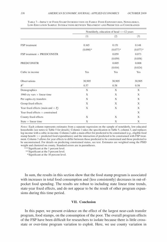
136 AmEriCAn EConomiC JournAL: APPLiED EConomiCS oCToBEr 2009
In sum, the results in this section show that the food stamp program is associated with increases in total food consumption and (less consistently) decreases in out-of-pocket food spending. The results are robust to including state linear time trends, state-year fixed effects, and do not appear to be the result of other program expan-sions during this time period.
VII. Conclusion
In this paper, we present evidence on the effect of the largest near-cash transfer program, food stamps, on the consumption of the poor. The overall program effects of the FSP have been difficult for researchers to isolate because there is little cross-state or over-time program variation to exploit. Here, we use county variation in
Table 7—Impact of Food Stamp Introduction on Family Food Expenditures, Nonelderly, Low-Education Sample: Interactions between Treatment and Predicted as Constrained
Nonelderly, education of head <=12 years
(1) (2) (3)
FSP treatment 0.165 0.151 0.148
(0.090)* (0.077)* (0.077)*FSP treatment × PREDCONSTR 0.059 0.073
(0.059) (0.058)PREDCONSTR 0.005 0.008
(0.014) (0.024)Cubic in income Yes Yes Yes
Observations 30,905 30,905 30,905
r2 0.57 0.58 0.58
Demographics X X X
1960 cty vars × linear time X X X
Per capita cty transfers X X X
Group fixed effects X X X
Year fixed effects (main and × Pg) X X X
Year fixed effects × constrained X
County fixed effects X X X
State × linear time X X X
notes: Each column represents estimates from a separate regression on the sample of nonelderly, low-educated households (see notes to Table 5 for details). Column 1 takes the specification in Table 5, column 3, and replaces log income with a cubic in income. Column 2 adds a main effect for predicted to be constrained (e.g., eligible food stamp benefit >= predicted food expenditures) and the interaction of predicted to be constrained with FSP treat-ment. Column 3 allows for year effects to differ between those predicted to be constrained and those predicted to be unconstrained. For details on predicting constrained status, see text. Estimates are weighted using the PSID weight and clustered on county. Standard errors are in parentheses.
*** Significant at the 1 percent level. ** Significant at the 5 percent level. * Significant at the 10 percent level.

VoL. 1 no. 4 137HoYnES AnD SCHAnZEnBACH: rESPonSES To in-KinD TrAnSFErS
the adoption of the program from 1963–1975 to identify the impact of food stamps. Using the PSID, we find that the FSP significantly increases food expenditures. By introducing and developing this research design, the paper provides an impor-tant contribution to the literature on evaluating the behavioral impacts of transfer programs.
Perhaps, more importantly, the paper tests the economics of in-kind transfers. Economic theory has strong predictions about how consumers will reallocate their spending in response to in-kind transfers. Despite the well-known theoretical pre-dictions, there has been relatively little empirical work to test those predictions. Our results, while mixed in statistical significance, are uniformly consistent with theo-retical predictions. First, the poor react to in-kind transfers by reducing their out-of-pocket spending on the targeted good (although these results are not statistically
Table 8—Impact of Food Stamp Introduction on Family Food Expenditures Sensitivity to Alternative Functional Form:
Nonelderly, education of head <= 12 years
Main estimates (log-log) semi-log linear quadratic
Specification for dep. var. log (total food) log (total food) total food exp. total food exp. total food exp.
Specification for income — — log (income) log (income) income quad. income
County FSP implemented × 0.208 0.238 0.169 1,512 1,513 1,499 group participation rate (0.096)** (0.097)** (0.090)* (762)** (767)** (764)*County FSP implemented −0.005 −0.024 0.004 −37 −56 −48
(0.020) (0.022) (0.019) (147) (148) (148)log (income) — — 0.290 1,875
(0.009)*** (68)***
income 0.038 0.051(0.002)*** (0.003)***
income2 (/$10,000) −0.001(0.000)***
Observations 30,905 30,677 30,905 30,905 30,905 30,905
r2 0.52 0.52 0.58 0.56 0.57 0.56
Estimated MPC food stamps 0.200 0.228 0.163 0.199 0.199 0.197
Estimated MPC income — — 0.087 0.077 0.038 0.048
Demographics X X X X X X
1960 cty vars × linear time X X X X X X
Per capita cty transfers X X X X X X
Group fixed effects X X X X X X
Year fixed effects (main and × Pg) X X X X X X
County fixed effects X X X X X X
State × linear time X X X X X
State × year fixed effects X
notes: Each column presents estimates from a regression of total food expenditures on a dummy variable equal to one if the county-year observation had a food stamp program in place by January of that year interacted with the group participation rate. The models differ with respect to the functional form (logs or levels for dependent vari-able, logs or levels for income) and whether they include state-year fixed effects. All other control variables and sample selection correspond to specification (1) in Table 5. See the notes to that table for more details. Standard errors are in parentheses. Estimates are weighted using the PSID weight and clustered on county. The marginal propensities to consume food are evaluated at mean values for food expenditures and family income among food stamp recipient families.
*** Significant at the 1 percent level. ** Significant at the 5 percent level. * Significant at the 10 percent level.

138 AmEriCAn EConomiC JournAL: APPLiED EConomiCS oCToBEr 2009
significant). Second, total consumption of the targeted good from all sources (cash outlays and in-kind transfers) increases. Third, providing food stamp benefits in voucher form leads to a minimal distortion of the consumption choice relative to what it would be if the benefit were provided in cash.
Our findings contribute to the literature in two distinct ways. First, we provide important and new estimates of the impact of the food stamp program on consumption using a credible research design. Second, we test predictions of the theory of consumer choice and, in particular, the differential impacts of cash versus in-kind transfers.
Even though there have been changes in the US population and the parameters of the FSP since the period we are studying, these results are relevant for today’s policy debates. To date, there have been no studies, that we have found, that provide credible evidence on the impact of the FSP on consumption and income. The FSP (recently renamed the Supplemental Nutrition Assistance Program) is once again receiving considerable political attention, and it is crucial from a policy maker’s perspective to be able to measure the benefits of the program, not only on food spending, but also on other outcomes like income, child well-being, and health.
REFERENCES
Acemoglu, Daron, David H. Autor, and David Lyle. 2004. “Women, War, and Wages: The Effect of Female Labor Supply on the Wage Structure at Midcentury.” Journal of Political Economy, 112(3): 497–551.
Almond, Douglas, Kenneth Y. Chay, and Michael Greenstone. 2006. “Civil Rights, the War on Pov-erty, and Black-White Convergence in Infant Mortality in the Rural South and Mississippi.” MIT Department of Economics Working Paper 07-04.
Almond, Douglas, Hilary W. Hoynes, and Diane Whitmore Schanzenbach. 2008. “Inside the War on Poverty: The Impact of Food Stamps on Birth Outcomes.” National Bureau of Economic Research Working Paper 14306.
Berry, Jeffrey M. 1984. Feeding Hungry People: rulemaking in the Food Stamp Program. New Brunswick, NJ: Rutgers University Press.
Bertrand, Marianne, Esther Duflo, and Sendhil Mullainathan. 2004. “How Much Should We Trust Differences-in-Differences Estimates?” Quarterly Journal of Economics, 119(1): 249–75.
Blanciforti, Laura, and Richard Green. 1983. “An Almost Ideal Demand System Incorporating Hab-its: An Analysis of Expenditures on Food and Aggregate Commodity Groups.” review of Eco-nomics and Statistics, 65(3): 511–15.
Bleakley, Hoyt. 2007. “Disease and Development: Evidence from Hookworm Eradication in the American South.” Quarterly Journal of Economics, 122(1): 73–117.
Blundell, Richard, and Luigi Pistaferri. 2003. “Income Volatility and Household Consumption: The Impact of Food Assistance Programs.” Journal of Human resources, 38(S): 1032–50.
Cascio, Elizabeth, Nora Gordon, Ethan Lewis, and Sarah Reber. Forthcoming. “Paying for Progress: Conditional Grants and the Desegregation of Southern Schools.” Quarterly Journal of Economics.
Citizens’ Board of Inquiry. 1968. Hunger, u.S.A.: A report by the Citizens’ Board of inquiry into Hunger and malnutrition in the united States. Boston: Beacon Press.
Currie, Janet. 2003. “U.S. Food and Nutrition Programs.” In means-Tested Transfer Programs in the united States, ed. Robert A. Moffitt, 199–290. Chicago: University of Chicago Press.
Currie, Janet. 2006. “The Take-Up of Social Benefits.” In Public Policy and the income Distribu-tion, ed. Alan J. Auerbach, David Card, and John M. Quigley, 80–148. New York: Russell Sage Foundation.
Currie, Janet, and Enrico Moretti. 2008. “Did the Introduction of Food Stamps Affect Birth Out-comes in California?” In making Americans Healthier: Social and Economic Policy as Health Policy, ed. Robert F. Schoeni, James S. House, George A. Kaplan, and Harold Pollack, 122–42. New York: Russell Sage Foundation.
Deaton, Angus S., and John Muellbauer. 1980. “An Almost Ideal Demand System.” American Eco-nomic review, 70(3): 312–26.

VoL. 1 no. 4 139HoYnES AnD SCHAnZEnBACH: rESPonSES To in-KinD TrAnSFErS
Eisinger, Peter K. 1998. Toward an End to Hunger. Washington, DC: Brookings Institution Press.Engen, Eric M., and Jonathan Gruber. 2001. “Unemployment Insurance and Precautionary Saving.”
Journal of monetary Economics, 47(3): 545–79.Finkelstein, Amy, and Robin McKnight. 2008. “What Did Medicare Do? The Initial Impact of Medi-
care on Mortality and Out of Pocket Medical Spending.” Journal of Public Economics, 92(7): 1644–68.
Fishback, Price V., and Shawn Everett Kantor. 1995. “Did Workers Pay for the Passage of Workers’ Compensation Laws?” Quarterly Journal of Economics, 110(3): 713–42.
Fraker, Thomas M. 1990. Effects of Food Stamps on Food Consumption: A review of the Literature. Washington, DC: Mathematica Policy Research, Inc.
Fraker, Thomas M., Alberto P. Martini, James C. Ohls, Michael Ponza, and Elizabeth A. Quinn. 1992. The Evaluation of the Alabama Food Stamp Cash-out Demonstration. Vol. 1: recipient impacts. Washington, DC: Mathematica Policy Research, Inc.
Gruber, Jonathan. 1997. “The Consumption Smoothing Benefits of Unemployment Insurance.” American Economic review, 87(1): 192–205.
Gruber, Jonathan. 2000. “Cash Welfare as a Consumption Smoothing Mechanism for Divorced Mothers.” Journal of Public Economics, 75(2): 157–82.
Gruber, Jonathan, and Aaron Yelowitz. 1999. “Public Health Insurance and Private Savings.” Jour-nal of Political Economy, 107(6): 1249–74.
Haider, Steven J., Alison Jacknowitz, and Robert F. Schoeni. 2003. “Food Stamps and the Elderly: Why Is Participation So Low?” Journal of Human resources, 38(S): 1080–1111.
Hubbard, R. Glenn, Jonathan Skinner, and Stephen P. Zeldes. 1995. “Precautionary Saving and Social Insurance.” Journal of Political Economy, 103(2): 360–99.
Kotz, Nick. 1969. Let them Eat Promises: The Politics of Hunger in America. New York: Doubleday.Levedahl, J. William. 1995. “A Theoretical and Empirical Evaluation of the Functional Forms Used
to Estimate the Food Expenditure Equation of Food Stamp Recipients.” American Journal of Agri-cultural Economics, 77(4): 960–68.
Ludwig, Jens, and Douglas L. Miller. 2007. “Does Head Start Improve Children’s Life Chances? Evi-dence from a Regression Discontinuity Design.” Quarterly Journal of Economics, 122(1): 159–208.
MacDonald, Maurice. 1977. Food, Stamps, and income maintenance. New York: Academic Press.Meyer, Bruce D., and James X. Sullivan. 2003. “Measuring the Well-Being of the Poor Using Income
and Consumption.” Journal of Human resources, 38(S): 1180–1220.Meyer, Bruce D., and James X. Sullivan. 2004. “The Effects of Welfare and Tax Reform: The Mate-
rial Well-Being of Single Mothers in the 1980s and 1990s.” Journal of Public Economics, 88(7–8): 1387–1420.
Moffitt, Robert. 1983. “An Economic Model of Welfare Stigma.” American Economic review, 73(5): 1023–35.
Ohls, James C., and Harold Beebout. 1993. The Food Stamp Program: Design Tradeoffs, Policy, and impacts. Washington, DC: Urban Institute Press.
Ohls, James C., Thomas M. Fraker, Alberto P. Martini, and Michael Ponza. 1992. The Effects of Cash-out on Food use by Food Stamp Program Participants in San Diego. USDA, Food and Nutrition Service, Office of Analysis and Evaluation.
Schanzenbach, Diane Whitmore. 2007. “What Are Food Stamps Worth?” Unpublished.Souleles, Nicholas S. 1999. “The Response of Household Consumption to Income Tax Refunds.”
American Economic review, 89(4): 947–58.Southworth, Herman M. 1945. “The Economics of Public Measures to Subsidize Food Consump-
tion.” Journal of Farm Economics, 27(1): 38–66.U.S. Congressional Budget Office. 1977. “The Food Stamp Program: Income or Food Supplementa-
tion?” Washington, DC: US Government Printing Office.U.S. Department of Agriculture, Food and Nutrition Service (various years). “Food Stamp Program,
Year-End Participation and Bonus Coupons Issues.” U.S. Department of Commerce. 1978. Bureau of Census. “City and County Data Bank, Consolidated
File: County Data, 1947–1977.”U.S. Department of Commerce. 2007. Bureau of Economic Analysis. http://www.bea.gov/bea/
regional/reis/. Whitmore, Diane. 2002. “Using the Food Stamp Cash-out to Test Intra-Household Bargaining.”
Unpublished.Zeldes, Stephen P. 1989. “Consumption and Liquidity Constraints: An Empirical Investigation.” Jour-
nal of Political Economy, 97(2): 305–46.