consumption and portfolio decisions when expected returns...

Consumption and Portfolio Decisions When Expected Returns Are Time VaryingAuthor(s): John Y. Campbell and Luis M. ViceiraSource: The Quarterly Journal of Economics, Vol. 114, No. 2 (May, 1999), pp. 433-495Published by: The MIT PressStable URL: http://www.jstor.org/stable/2587014Accessed: 22/02/2009 15:22

Your use of the JSTOR archive indicates your acceptance of JSTOR's Terms and Conditions of Use, available athttp://www.jstor.org/page/info/about/policies/terms.jsp. JSTOR's Terms and Conditions of Use provides, in part, that unlessyou have obtained prior permission, you may not download an entire issue of a journal or multiple copies of articles, and youmay use content in the JSTOR archive only for your personal, non-commercial use.

Please contact the publisher regarding any further use of this work. Publisher contact information may be obtained athttp://www.jstor.org/action/showPublisher?publisherCode=mitpress.

Each copy of any part of a JSTOR transmission must contain the same copyright notice that appears on the screen or printedpage of such transmission.

JSTOR is a not-for-profit organization founded in 1995 to build trusted digital archives for scholarship. We work with thescholarly community to preserve their work and the materials they rely upon, and to build a common research platform thatpromotes the discovery and use of these resources. For more information about JSTOR, please contact [email protected].

The MIT Press is collaborating with JSTOR to digitize, preserve and extend access to The Quarterly Journal ofEconomics.

http://www.jstor.org

http://www.jstor.org/stable/2587014?origin=JSTOR-pdf

http://www.jstor.org/page/info/about/policies/terms.jsp

http://www.jstor.org/action/showPublisher?publisherCode=mitpress

434 QUARTERLY JOURNAL OF ECONOMICS

not hold. Expected asset returns seem to vary through time so that investment opportunities are not constant; the evidence for predictable variation in the equity premium, the excess return on stock over Treasury bills, is particularly strong (see Campbell [1987]; Campbell and Shiller [1988a, 1988b]; Fama and French [1988, 1989]; Hodrick [1992]; or the textbook treatment in Camp- bell, Lo, and MacKinlay [1997, Chapter 7]). Economists research- ing the equity premium puzzle find that average excess stock returns are too high to be consistent with a representative- investor model in which the investor has log utility (see Campbell [1996]; Cecchetti, Lam, and Mark [1994]; Cochrane and Hansen [1992]; Hansen and Jagannathan [1991]; Kocherlakota [1996]; Mehra and Prescott [1985]; or the textbook treatment in Camp- bell, Lo, and MacKinlay [Chapter 8]).

In response to these empirical findings, several recent papers have used numerical methods to solve for optimal portfolios in models with realistic predictability of returns. Investors are generally assumed to have power utility defined over wealth at a single terminal date. Different papers choose different investment horizons and make different assumptions about investors' ability to rebalance their portfolios. Kandel and Stambaugh [1996] consider the effects of predictability on the optimal portfolio of a single-period Bayesian investor who takes account of parameter uncertainty, while Barberis [1999] extends this work to study the optimal portfolio of a long-horizon Bayesian investor who rebalances annually or not at all. Brennan, Schwartz, and Lagnado [1997] consider a long-horizon investor who rebalances frequently, while Balduzzi and Lynch [1997a, 1997b] consider a long-horizon investor who faces fixed and proportional transactions costs which reduce the frequency of optimal rebalancing.1 The results in these papers, though dependent on the particular parameter values they assume, illuminate the effects of predictability on portfolio choice. Kim and Omberg [1996] work with a similar framework but, by assuming continuous time and zero transactions costs, are able to solve the portfolio choice problem analytically.2

A limitation of these models is that they abstract from the

1. Most of these papers, like our paper, work with a single state variable driving the equity premium. Only Brennan, Schwartz, and Lagnado [1997] consider multiple state variables.

2. Kim and Omberg study the choice between a riskless asset with a constant return and a risky asset whose expected return follows a continuous-time AR(1) (Ornstein-Uhlenbeck) process. They assume that the investor is finitely lived and

CONSUMPTION AND PORTFOLIO DECISIONS 435

choice of consumption over time. Since the investor is assumed to value only wealth at a single terminal date, no consumption takes place before the terminal date, and all portfolio returns are reinvested until that date. This simplifies the analysis but makes it hard to apply the results to the realistic problem facing an investor saving for retirement. In addition, these models cannot easily be related to the macroeconomic asset pricing literature in which consumption is used as an indicator of marginal utility.

This paper extends the previous literature in three major respects. First and most important, we consider a model in which a long-lived investor chooses consumption as well as an optimal portfolio, to maximize a utility function defined over consumption rather than wealth.3 Second, we assume that the investor has Epstein-Zin-Weil preferences [Epstein and Zin 1989; Weil 1989]. This allows us to distinguish the coefficient of relative risk aversion from the elasticity of intertemporal substitution in consumption; power utility restricts risk aversion to be the reciprocal of the elasticity of intertemporal substitution, but in fact these parameters have very different effects on optimal consumption and portfolio choice. Third, like Kim and Omberg [1996] but unlike other previous research, we solve the problem analytically. This provides economic insights that are hard to get from numerical solutions, and it enables us to distinguish general properties of the solution from results that depend on particular parameter values.

In order to keep our problem analytically tractable, we make several simplifying assumptions. We assume that there are two assets: a riskless asset with a constant return, and a risky asset whose expected return, the single state variable for the problem, follows a mean-reverting AR(1) process. The assumption that the riskless return is constant simplifies our analysis and enables us to isolate the effects of time variation in the equity premium.

We work in discrete time, and assume that the investor is able to rebalance the portfolio every period. Our approximate solution method becomes more accurate as the period length shrinks; thus,

has HARA utility defined over terminal wealth. They find that the optimal portfolio weight is linear and the value function is quadratic in the state variable.

3. Since the first version of this paper was circulated, some numerical results have been obtained for the long-horizon portfolio choice problem with utility defined over consumption. Balduzzi and Lynch [1997a, 1997b] consider some cases with endogenous consumption, and Brandt [1999] uses the Generalized Method of Moments to estimate consumption and portfolio rules that best satisfy the intertemporal Euler equation given the stochastic properties of historical data.


our model applies to an investor who is able to rebalance frequently. We also abstract from transactions costs and restrictions on borrowing or short sales. We make these assumptions not only for tractability, but also because we want to focus on the pure intertemporal effects of return predictability on optimal consumption and portfolio choice for long-horizon investors. Transactions costs and portfolio restrictions, while interesting in their own right, may obscure these effects.

Finally, we assume that the investor is infinitely lived. In a model with endogenous consumption every period, Fischer [1983] notes that "the notion of the horizon loses its crispness. Date T is still the horizon in the sense that the individual looks no further ahead than T. But now events that occur at t < T matter not only because they affect the situation at T but also because consumption at t and later depends on the state of the world at time t" [p. 155]. An infinite horizon is particularly convenient analytically because the problem becomes one of finding a fixed point rather than solving backward from a distant terminal date. It may be an appropriate assumption for investors with bequest motives, as discussed in the macroeconomic literature on Ricardian equiva- lence, and it approximates well the situation of investors with finite but long horizons.4

The endogeneity of consumption in our model makes it impossible for us to follow Kim and Omberg [1996] and derive an analytical solution that is exact for all parameter values.5 Instead, we find an approximation to the portfolio choice problem that can be solved using the method of undetermined coefficients. We approximate the Euler equations of the problem using second- order Taylor expansions, and we replace the investor's intertemporal budget constraint with an approximate constraint that is linear in log consumption and quadratic in the portfolio weight on the risky asset. This enables us to find approximate analytical solutions for consumption and the portfolio weight. Like Kim and

4. Brandt [1998] compares his finite-horizon results to ours. For the parameter values he uses, the finite-horizon solution converges quickly to the infinite- horizon solution and is very similar by the time the finite horizon reaches twenty years.

5. The lack of an exact analytical solution is not due to the fact that we work in discrete time. Schroder and Skiadas [1998] use stochastic differential utility, a continuous-time version of Epstein-Zin-Weil preferences due to Duffie and Epstein [1992], and show that it is possible to characterize the solution in terms of quasi-linear parabolic partial differential equations-which are relatively easy to solve numerically-but an exact closed-form solution exists only in the same special cases as in discrete time.


Omberg [1996] we find that the optimal portfolio weight is linear in the state variable, while the log consumption-wealth ratio and the log value function are quadratic in the state variable.

The approximate solution holds exactly in some special, but important, cases noted by Giovannini and Weil [1989]. In all other cases its accuracy is an empirical issue. Campbell, Cocco, Gomes, Maenhout, and Viceira [1998] compare the approximate analytical solution to a discrete-state numerical solution, and find that the two are very similar except at the upper extreme of the state space. We briefly summarize these findings in subsection IV.6 of this paper.

Our solution method uses the intertemporal Euler equation as its starting point. In this sense, it belongs to the class of stochastic dynamic programming methods. Cox and Huang [1989] have proposed an alternative solution method which transforms an intertemporal optimization problem with complete markets into an equivalent static optimization problem that can be solved using standard Lagrangian theory. He and Pearson [1991] have extended the Cox-Huang approach to settings with incomplete markets. In a related paper [Campbell and Viceira 1998] we formulate a problem of optimal consumption and portfolio choice with time-varying interest rates, constant risk premiums, and complete markets, and we explore the relation between the log-linear approximate solution method and the Cox-Huang approach.

Our paper builds on the work of Campbell [1993]. Campbell considers the simpler problem where only one asset is available for investment and so the agent need only choose consumption. He shows that this problem becomes tractable if one replaces the intertemporal budget constraint by a log-linear approximate constraint. He uses the solution in a representative-agent model to characterize the equilibrium prices of other assets that are in zero net supply, in the spirit of Merton's [1973] intertemporal CAPM. Campbell [1996] estimates the parameters of the model from U. S. asset market data, while Campbell and Koo [1997] evaluate the accuracy of the approximate analytical solution by comparing it with a discrete-state numerical solution.

The organization of the paper is as follows. Section II states the problem we would like to solve, while Section III explains our approximate solution method. Section IV calibrates the model to postwar quarterly U. S. stock market data and briefly discusses


intertemporal substitution, and the parameter 0 is defined as 0 = (1 - -y)/(l - ij-1). It is easy to see that (6) reduces to the standard time-separable, power utility function with relative risk aversion -y when p = -y-1. In this case 0 = 1, and the nonlinear recursion (6) becomes linear.

(A5). The investor is infinitely lived. Assumptions (Al) and (A2) on the number of risky assets and

state variables are simplifying assumptions, which we adopt for expositional purposes. The approach of this paper can be applied to a more general setting with multiple risky assets and state variables, at the cost of greater complexity in the analytical solutions to the problem. Assumption (A3) is also a simplification that can be relaxed in order to study the effects of conditional heteroskedasticity on portfolio choice. Assumption (A4) on preferences allows us to separate the effects on optimal consumption and portfolio decisions of the investor's attitude toward risk from the investor's attitude toward consumption smoothing over time. Finally, assumption (A5) allows us to ignore the effects of a finite horizon on portfolio choice, but this assumption too can be relaxed in future work.

11.2. Euler Equations and the Value Function

The individual chooses consumption and portfolio policies that maximize (6) subject to the budget constraint,

(7) Wt+1 = Rpt+l(Wt - cd,

where Wt is total wealth at the beginning of time t and Rp,t+1 is the return on wealth (1).

Epstein and Zin [1989, 1991] have shown that with this form for the budget constraint, the optimal portfolio and consumption policies must satisfy the following Euler equation for any asset i:

(8) 1 =Et[I ( C | )Ri .

Equation (8) holds regardless of how many tradable assets are available. In our simple model, i denotes the riskless asset, the single risky asset, or the investor's portfolio p. When i = p, (8) reduces to

(9) 1 = Et[I8 (C+;i) RPlAR jO]


Hence, U1,C-Wt depends on the individual's future portfolio and consumption decisions, and (19) falls short of a complete solution to the model.

III.4. Solving for the Optimal Policies

The final step in solving the dynamic optimization problem is to guess a functional form for the optimal consumption and portfolio policies and to identify the parameters of these policies using the method of undetermined coefficients. We guess that the optimal portfolio weight on the risky asset is linear in the state variable, and that the optimal log consumption-wealth ratio is quadratic in the state variable. Hence, we guess that

(i) ott = ao + alxt,

(ii) ct - wt = bo + blxt + b2xt,

where jao,aj,b0,bj,b2} are fixed parameters to be determined. Under assumptions (A1)-(A5) we can show that guesses

(i)-(ii) are indeed a solution to the intertemporal optimization problem of the recursive-utility-maximizing investor, and we can solve for the unknown parameters jao,aj,bo,bj,b2}. Details are provided in Appendices 1 and 2; here we give a brief intuitive explanation of the solution.

The linear portfolio rule (i) has the simplest form consistent with time variation in the investor's portfolio decisions. This portfolio rule implies that the expected return on the portfolio is quadratic in the state variable xt, because an increase in xt affects the expected portfolio return both directly by increasing the expected return on existing risky-asset holdings and indirectly by changing the investor's optimal allocation to the risky asset. Equation (20) shows that the log consumption-wealth ratio is linearly related to the expected portfolio return, so it is natural to guess that the log consumption-wealth ratio is quadratic in the state variable xt.

Of course, variances and covariances of consumption growth and asset returns also affect the optimal consumption and portfolio decisions. But the homoskedastic linear AR(1) process for xt implies that all relevant variances and covariances are either linear or quadratic in the current state variable, and thus second-moment effects do not change the linear-quadratic form of the solution. Appendix 1 states nine lemmas that express important expectations, variances, and covariances as linear or quadratic functions of the state variable.


We now state two propositions that enable us to solve for the unknown coefficients of the model. The propositions are proved in Appendix 2, using the lemmas from Appendix 1.

PROPOSITION 1. The parameters defining the linear portfolio policy (i) satisfy the following two-equation system:

a o (= 2)( Y 1) Wr _ _ _ _ _ _

ai = (2 ) - _ Y -_2 -1 - 1 2

al = - )-( _) 2(+.

Proof of Proposition 1. See Appendix 2.

The first term in each of these equations is the myopic component of asset demand in equation (19). Therefore, the remaining terms represent intertemporal hedging demand. They depend on the consumption coefficients b1 and b2, divided by one minus the intertemporal elasticity of substitution (1 - tp), as well as on the scaled deviation of risk aversion from one, (-y - 1)/by, and the scaled covariance of the risky asset return with revisions in the expected future return uqu/u 2. There is no hedging demand if this covariance is zero, for then the risky asset cannot be used to hedge changes in investment opportunities. We discuss the effects of these parameters on portfolio selection in more detail in our calibration exercise in Section IV.

Proposition 1 expresses the coefficients of the optimal portfolio policy as linear functions of the parameters of the optimal consumption rule. Proposition 2 shows that these parameters solve a recursive, nonlinear equation system whose coefficients are known constants:

PROPOSITION 2. The parameters defining the consumption policy (ii), 1b0,b1,b21, are given by the solution to the following recursive nonlinear equation system:

(21) 0 = A10 + A11bo + A12b1 + A13bl + A14b2

+ 1 + 16bjb2,

(22) 0 = A20 + A21b, + A22b2 + A23b2 + A24bb2,

(23) 0 = A30 + A31b2 + A32b2,


where Aij; i= 1,2,3,j= 1, . . ., 61 are constants given in Appendix 2. These constants depend on the exogenous parameters of the model and on the log-linearization parameter p.

Proof of Proposition 2. See Appendix 2.

The equation system given in Proposition 2 can be solved recursively, starting with the quadratic equation (23) whose only unknown is b2. This equation has two possible roots, which are always real when -y - 1, and are real when -y < 1 if

-(,2 - (l/p))2(T2 + (1 - )(+2 - (1/p))4(aq]u - (1 - -y)4+2U2 2, 0. The existence of real roots is necessary (but not sufficient) for the value function of the problem, given in Property 1 below, to be finite. We argue in the next section that one of the two roots, the positive root of the equation discriminant, delivers the correct solution to the model.

Once we have solved for b2, the second equation in the system becomes a linear equation in b1. Finally, given 1b1,b21, the first equation of the system is also linear in bo. Using the known values of {b0,b1,b2j in Proposition 1, we can find lao,ail.

All of these calculations are conditional on a value for p, since p helps to determine the constants Aij in (21), (22), and (23). One can write the parameters as functions of p, for example bo(p), b1(p), and b2(p), to express this dependence. But p itself depends on the optimal expected log consumption-wealth ratio and hence on the parameters: p = 1 - exp IE(ct - wt)l = 1 - exp lbo(p) + b1(p)jt + b2(p)(jt2 + o.2)J. The solution of the model is complete only when a value of p has been found to satisfy this nonlinear equation. Unfortunately, an analytical solution is available only in the case t+ = 1, where the optimal consumption policy is myopic and p = 6. In all other cases, we resort to a numerical method. We first set p = 8 and then find the optimal values of {a0,aj,b0,b1,b21 given this value of p. For these optimal values we then compute E(ct - wt) and a, new value of p, for which a new set of optimal policies is computed. We proceed with this recursion until the absolute value of the difference between two consecutive values of p is less than lO-4.

This procedure converges extremely rapidly whenever there exists a solution for p between zero and one. For some parameter values, however, p converges to one, and the implied value function of our model is infinite. It is well-known that this can occur in infinite-horizon optimization problems; Merton [1971]


and Svensson [1989], for example, derive parameter restrictions that are required for finite value functions in continuous-time models with constant expected returns. Unfortunately, the nonlin- earity of the equation for p prevents us from deriving equivalent analytical restrictions in our model with time-varying expected returns, but the problem tends to arise whenever the utility discount rate is too low or the expected excess equity return is too high on average or too variable relative to the risk of equity investment.

III.5. Properties of the Solution

Propositions 1 and 2 identify the parameters of the optimal policies and the value function per unit of wealth. If we pick the solution for b2 given by the positive root of the discriminant in (23), Propositions 1 and 2 also imply the following properties of the solution. Here we merely state these properties; proofs are given in Appendix 3.

PROPERTY 1. The approximate value function per unit of wealth is given by

(bo - ) { log (1 - ) bi b2 }

and b2/(1 - t]) > 0. Therefore, the value function per unit of wealth is a convex function of xt, the expected log excess return on the risky asset.

PROPERTY 2. The slope of the optimal portfolio rule-the coefficient a,-is positive. Also, lim. ax a, = 0 and lim-_0 a, = +xo.

Property 1 characterizes the approximate value function per unit of wealth. Equation (24) shows that the log value function per unit of wealth is a quadratic function of the state variable whose coefficients are the coefficients of the log consumption-wealth function divided by one minus the elasticity of intertemporal substitution.8

Property 1 tells us that the value function per unit of wealth is convex in xt, so it increases with xt when xt is large enough and

8. This expression has a well-defined limit as i - 1. The solutions to equations (22) and (23) imply that b/(1 - tI) and b2/(1 - I) are functions only of p and -y, and do not depend directly on W. Property 3 shows that p = 8 when ' - 1. Finally, equation (21) implies that (bo - vi log (1 - 8))/(1 - vI) does not depend directly on t+ when p = 8. Thus, (24) is well defined as ' - 1.


decreases with xt when xt is small enough. The intuition for this result is as follows. The investor can profit from predictable excess returns on the risky asset, whether these are positive or negative. Property 2 implies that the investor increases the allocation to the risky asset as its expected excess return increases. If excess returns are expected to be sufficiently positive, the investor will profit by going long; whereas if they are expected to be sufficiently negative, the investor will profit by going short. Thus, movements in xt to extreme positive or negative values increase the investor's utility.

Property 2 generalizes a known comparative-statics result for an investor with power utility facing constant expected returns in a continuous-time model. In that setting the allocation to the risky asset is constant over time, and it increases with the expected excess return on the risky asset. In static models with more general utility functions, however, it is possible for the allocation to the risky asset to decline with the expected excess return on the risky asset, because the income effect of an increase in the risk premium can overcome the substitution effect [Ingersoll 1987, Chapter 3]. Property 2 shows that this does not happen in our dynamic model with Epstein-Zin-Weil utility. The coefficient a, is always positive and increases from zero when My is infinitely large to infinitely large values as My approaches zero.

PROPERTY 3. The solution given by Propositions 1 and 2 approaches known, exact solutions as the parameters of utility approach the following special cases:

a) When t] = 1 and My - 1, equation (23) becomes linear and b2/ - 0) - 1/2 2>(1/p - +2) > 0. In this case, the optimal portfolio rule is myopic: ao 1 l/2-y and a, 1b/yo2. This portfolio rule is the known, exact solution of Giovannini and Weil [1989], in which portfolio choice is myopic even though consumption choice is not. The portfolio rule maximizes the conditional expectation of the log return on wealth.

b) When t- 1 and -y f 1, b, 0, b2 0, p 8, and bo log (1 - 6). This consumption rule is the known, exact solution of Giovannini and Weil [1989], in which consumption choice is myopic-in the sense that the consumption- wealth ratio is constant-even though the optimal portfolio rule is not.


c) When ] - 1 and My 1, so that utility is logarithmic, b, -

0, b2 0 0, p - 8, bo log (1 - 6), ao - 1/2, and a, -- 1/of. This is the known, exact solution for log utility in which both the optimal consumption rule and the optimal portfolio rule are myopic.

d) When a 2 0, so that expected returns are constant, both the optimal consumption rule and the optimal portfolio rule converge to the known, exact, myopic solution. The portfolio parameters ao - 1/2-y and a, 1/-y1y.

It is important to note that the previously known results mentioned in parts a) and b) of Property 3 are only partial. That is, the exact portfolio rule is known for the case My = 1, but our approximate solution method is still needed to determine the optimal consumption rule. The exact consumption rule is known for the case tp = 1, but our solution method is still needed to determine the optimal portfolio rule. In this case our solution is exact (in continuous time) since the optimal consumption-wealth ratio is constant so our log-linear version of the intertemporal budget constraint holds exactly.

Property 3 holds only if we choose the positive root of the discriminant in the quadratic equation for b2, (23). If instead we choose the negative root of the discriminant, the approximate solutions diverge as the preference parameters approach the known special cases. This is our main reason for choosing the positive root of the discriminant.9

PROPERTY 4. The optimal portfolio rule does not depend on t] for given p.

This property holds because only the ratios b1/(l - t]) and b2/(l- t]) appear in the portfolio rule, and these ratios do not depend on i for given p. The property shows that the main preference parameter determining portfolio choice is the coefficient of relative risk aversion My and not the elasticity of intertemporal substitution Wp. Conditioning on p, t+ has no effect on portfolio

9. We would like to be able to show analytically that the unconditional mean of the value function, a measure of welfare we study in Section V below, is always higher when we choose the positive root of the discriminant in (23). Unfortunately, we have been unable to do this; but in our calibration exercise we have verified that the positive root always gives the higher unconditional mean for every set of parameter values we consider. We do have a stronger analytical result when -y < 1. In this case the negative root of the discriminant violates a necessary and sufficient condition (derived by straightforward extension of the results of Constan- tinides [1992]) for the existence of the unconditional mean of the value function.


choice. However, p itself is a function of W-recall that p = 1 - exp {E[ct - wt]1-so the optimal portfolio rule depends on tp indirectly through p. Our calibration results in Section IV show that this indirect effect is small.

PROPERTY 5. The parameters a, and b2, the slope of the portfolio policy, and the curvature of the consumption policy, do not depend on jt for given p.

Property 5 shows that some aspects of the optimal policy-the sensitivity of the risky asset allocation to the state variable and the quadratic sensitivity of consumption to the state variable -

are independent of the average level of the excess return on the risky asset. Of course, other aspects-the average allocation to the risky asset, the average consumption-wealth ratio, and the linear sensitivity of consumption to the state variable -do depend on the average risk premium. We discuss this dependence in greater detail in subsection IV.3.

IV. CALIBRATION EXERCISE

IV1. Data and Estimation

An important advantage of our approach is that we can calibrate our model using real data on asset returns. To illustrate this, we use quarterly U. S. financial data for the sample period 1947.1-1995.4.10 In our calibration exercise, the risky asset is the U. S. stock market, and the risk-free asset is a short-term debt instrument. To measure stock returns and dividends, we use quarterly returns, dividends, and prices on the CRSP value- weighted market portfolio inclusive of the NYSE, AMEX, and NASDAQ markets. The short-term nominal interest rate is the three-month Treasury bill yield from the Risk Free File on the CRSP Bond tape. To compute the real log risk-free rate, the beginning-of-quarter nominal log yield is deflated by the end-of- quarter log rate of change in the Consumer Price Index from the Ibbotson files on the CRSP tape. Log excess returns are computed as the end-of-quarter nominal log stock return minus the beginning-of-quarter log yield on the risk-free asset.

10. A similar exercise using annual U. S. data for the period 1872-1993 is reported in the NBER Working Paper version of this article [Campbell and Viceira 1996].


The state variable is taken to be the log dividend-price ratio, measured as the log of the total dividend on the market portfolio over the last four quarters divided by the end-of-period stock price. Campbell and Shiller [1988a], Fama and French [1988], Hodrick [1992], and others have found this variable to be a good predictor of stock returns. We estimate the following restricted VAR(1) model:

rltl- rf' /00 El/01t (E

(25) - + (01 -dt pt) + dt+1i Pt+i \1O/ 4Pi E2,t+lI

where (Et+l,E2,t+1) - N(Oj), and report the maximum likelihood estimation results in Table I. Since (25) is equivalent to a multivariate regression model with the same explanatory variables in all equations, ML estimation is identical to OLS regression equation by equation. The standard errors for the slopes, intercepts, and the residual variance-covariance matrix are based on Proposition 11.2 in Hamilton [1994]; using these standard errors, which assume that the variables in the model are stationary, the slopes and the elements of the variance-covariance matrix all appear to be statistically different from zero.1"

The parameters in (3), (4), and (5) that define the stochastic structure of our model can be recovered from the VAR system (25) as follows: t = 0o + 01io/(l - P13), pig 13i, o] 02Q22, vu = , and

9,qu = OJ112. Table I reports these implied parameters along with standard errors computed using the delta method. All of the derived parameters except ark are significantly different from zero at the 5 percent confidence level. The unconditional expected log excess return jt is estimated at 5 percent per year (1.25 percent per quarter), while the log real risk-free rate rf is a meager .28 percent per year. 12

1V2. Solution of the Model

Using the parameter estimates in Table I, we compute the individual's optimal portfolio allocation and consumption-wealth ratio for a range of values of relative risk aversion and elasticity of

11. Note, however, that 1i is close to one. Elliott and Stock [1994] have shown that the t-ratio for 0 under the null Ho: 0 = 0 does not have a standard asymptotic normal distribution when the log dividend-price ratio follows a unit-root or near-unit-root process, and fQ12 = 0. We do not pursue this issue further here, and proceed to calculate standard errors under the assumption that the estimated system is stationary, but we note that standard errors computed under this assumption should be treated with some caution.

12. These parameter estimates differ slightly from those reported in the NBER Working Paper version of this article. The reason is that there, because of a computational error, we used the dividend-price ratio instead of its log when estimating (25).


and consumption rules implied by low and high risk aversion coefficients. We consider low elasticities of intertemporal substitution, both because we want to include the power-utility cases in which the elasticity of intertemporal substitution is the reciprocal of risk aversion, and because a low elasticity of intertemporal substitution seems to be required to explain the insensitivity of consumption growth to real interest rates in postwar U. S. data [Hall 1988, Campbell and Mankiw 1989].

Tables II, III, and IV and Figures I and II report the results of this exercise. To make it easier to interpret our results, we normalize the parameters defining the optimal portfolio and consumption policies (i) and (ii), so that the intercepts of the optimal policy functions are the optimal allocation to stocks and the optimal consumption-wealth ratio when the expected simple excess return, Et[R1,t~l] - Rf, is zero. At this point in the state space the risky asset is a "fair gamble" offering no risk premium. Thus, a myopic risk-averse investor would allocate no wealth to it, and all the demand for the risky asset is intertemporal hedging demand. The expected simple excess return is zero when the expected log excess return xt is equal to -of/2. Therefore, the parameters reported in the tables are a*, a,, b*, b j, and b2 in

(26) Ott = a* + al(xt + o2 /2)

and

(27) ct - Wt = b* + b* (xt + (U2 /2)) + b2(xt + (2u/2))2,

where a* = ao - a1(o2/2), bt = bo - b1(T2 /2) + b2 (G4/4), b* = b, - b2ff2, and a1 and b2 do not have asterisks because they coincide with the original parameters.

The main diagonal of each panel in the tables corresponds to standard power-utility preferences, since the elasticity of intertemporal substitution is the reciprocal of risk aversion along the main diagonal. The numbers reported in the tables summarize the optimal decisions of a recursive-utility individual who observes the true process for returns. Since we do not observe the true process but must estimate it, we have also computed-but we do not report here to save space-the standard errors for these parameters, using the delta method.13 These standard errors

13. The delta method requires the computation of derivatives of the parameters of interest (for example, a,) with respect to 1oo,oi3op3,f}. Since no analytical formulas are available, we use two-sided numerical derivatives based on a proportional perturbation parameter equal to 10-4. The standard errors are reported in the NBER Working Paper version of this article.


TABLE II OPTIMAL PORTFOLIO POLICY

R.R.A. E.I.S.

(A) Exponentiated intercept: ao x 100

11.75 1.00 1/1.5 1/2 1/4 1/10 1/20 1/40 0.75 -38.6 -29.4 -23.4 -21.0 - 18.2 - 16.7 -16.2 -16.0 1.00 0.0 0.0 0.0 0.0 0.0 0.0 0.0 0.0 1.50 27.1 23.5 20.5 19.2 17.5 16.6 16.3 16.2 2.00 33.8 30.7 27.9 26.6 24.8 23.9 23.6 23.5 4.00 29.9 29.8 29.7 29.6 29.5 29.4 29.4 29.4

10.00 16.0 17.2 18.5 19.2 20.4 21.2 21.4 21.6 20.00 8.8 9.7 10.8 11.4 12.4 13.1 13.3 13.4 40.00 4.6 5.2 5.8 6.2 6.8 7.3 7.4 7.5

(B) Slope: a,

1/.75 1.00 1/1.5 1/2 1/4 1/10 1/20 1/40 0.75 222.5 225.1 227.3 228.3 229.6 230.4 230.6 230.7 1.00 188.8 188.8 188.8 188.8 188.8 188.8 188.8 188.8 1.50 145.5 144.4 143.3 142.9 142.2 141.8 141.7 141.7 2.00 118.5 117.5 116.6 116.1 115.5 115.1 115.0 115.0 4.00 68.1 68.1 68.0 68.0 68.0 67.9 67.9 67.9

10.00 29.9 30.3 30.7 30.9 31.3 31.5 31.6 31.6 20.00 15.5 15.8 16.1 16.3 16.6 16.8 16.8 16.8 40.00 7.9 8.1 8.3 8.4 8.6 8.7 8.7 8.7

Panel A reports the optimal percentage allocation to stocks when the expected gross excess return is zero for different levels of relative risk aversion and elasticities of intertemporal substitution. Panel B reports the change-in percentage points-in the optimal allocation to stocks when the expected log excess return increases by 1 percent per quarter. These numbers are all based on the parameter estimates for the return process reported in Table II (sample period 1947:1-1995:4). The values on the main diagonal correspond to the power utility case.

show that the intercepts of the optimal policies are estimated with less precision than the parameters determining the slope and curvature of the optimal policy.

1V3. The Optimal Portfolio Rule

Tables II Ind III and Figure I summarize the optimal portfolio decision. Panel A in Table II reports a*, the optimal allocation to stocks when the expected gross excess return is zero, while Panel B in the same table reports a,, the slope of the optimal portfolio policy. Panel A in Table III reports the average total demand for stocks as a fraction of wealth, while Panel B reports the share of this average total demand that is attributable to the average hedging demand for stocks.

Figure I, which is divided into four panels, illustrates the portfolio rule at. Figure Ia fixes Wp at 1/0.75 and plots (t for a wide


across rows of the tables, as -y changes, is far greater than the variation across columns, as 4i changes. Similarly, the ott lines in Figures Ic and Id are all close together, whereas those in Figures Ia and Ib vary widely in both slope and intercept. This result can be understood by recalling Property 4 of our solution; i.e., that ott depends on 4i only through the dependence of p on 4i. Our calibration results show that this indirect effect through p is very small.

Panel A in Table II shows that the intercept of at, a*, is positive when -y > 1. It is zero when -y = 1, as we already know from the analysis of the special case with unit relative risk aversion, and negative when y < 1. These results hold regardless of the value of Wp. To interpret this behavior, recall that a * is the optimal allocation to stocks when the expected excess gross return is zero. Since the myopic demand for stocks is zero at this level of the expected excess gross return, a o is completely determined by hedging demand. Thus, at the point in the state space where the risky asset has a zero expected excess return, the sign of hedging demand is positive for investors with -y > 1.

Panel B in Table II shows that the coefficient a,, the slope of the at function, is positive for all levels of -y and 4i as implied by Property 2 of our solution. Like the intercept a*, the slope a, varies substantially across -y for a given level of 4, but changes very little across 4i for a given level of -y. As -y increases, a, rapidly approaches zero, indicating that the optimal portfolio rule is very responsive to changes in expected excess returns when the individual is close to risk-neutral but is almost flat when the individual is highly risk- averse. This finding is also implied by Property 2 of our solution.14

Panel B in Table II also shows that whenever -y > 1, intertemporal hedging demand increases the slope of the portfolio rule; equivalently, hedging demand itself has a positive slope. To see this, note that when -y = 1, hedging demand is zero and the slope coefficient of 188.8 is entirely attributable to the myopic component of asset demand. For higher values of -y, the myopic slope shrinks in proportion to -y. Thus, it is 94.4 for -y = 2, 47.2 for -y = 4, and so forth. The slope coefficients reported in Panel B in Table II shrink more slowly than this, implying a positive slope contribution from hedging demand. The analytical foundation of this result is that from Proposition 1 the slope of hedging demand

14. The standard errors not reported here show that the slope coefficient a, is much more precisely estimated than the intercept of the optimal portfolio rule. One reason for this greater precision is that, as we showed in Property 5, the slope of the portfolio rule is not sensitive to the mean excess stock return y whereas the intercept does depend on y.


is -(b2/(l - OA)Y - 1)/Y)(Uqu/u2)2, which is positive when -y > 1 under our assumption of negative |u. This implies that conservative long-horizon investors who are free to rebalance every period are actually more aggressive market timers than conservative short-horizon investors.15

The results in Table II can be explained in intuitive terms as follows. We have estimated a return-generating process which has a negative sign for uq, the covariance between unexpected stock returns and revisions in expected future stock returns. This implies that stocks tend to have high returns when their expected future returns fall. Since the investor is normally long in stocks, a decline in expected future stock returns is normally a deterioration in the investment opportunity set. There are offsetting considerations that determine an investor's attitudes toward assets that pay off when the investment opportunity set deterio- rates. On the one hand, an investor with low risk aversion (y < 1) wants to hold assets that deliver wealth when wealth is most productive; that is, when investment opportunities are good. This investor has a negative hedging demand. On the other hand, an investor with high risk aversion (by > 1) wants to hold assets that deliver wealth in unfavorable states of the world; that is, when investment opportunities are poor. This investor has a positive hedging demand. Interestingly, the hedging demand is not mono- tonic in risk aversion because an extremely risk-averse investor limits her exposure to the risky asset in all states of the world. Thus, the magnitude of hedging demand first rises and then falls with the coefficient of risk aversion.

Although the investor is normally long in stocks, if the expected excess return becomes sufficiently negative, a decline in expected future stock returns can represent an improvement in the investment opportunity set because it creates a profitable opportunity to short stocks. At this point in the state space, the sign of hedging demand for stocks reverses. This explains why hedging demand has both a positive intercept and a positive slope, allowing a sign reversal of hedging demand for sufficiently negative Xt.16

The average level of excess simple stock returns, jt + vu/2, plays an important role in this argument. We have estimated j + oU/2 to be positive and quite large; this leads the investor normally to maintain a long position in stocks for which a

15. Barberis [1999] finds that conservative buy-and-hold investors who know the parameters of the stock return process are about equally aggressive market timers whether they have a short or a long horizon.


decrease in the expected stock return represents a deterioration in investment opportunities. If j + vu2/2 were negative, however, the investor would normally have a short position in stocks for which a decrease in the expected stock return represents an improvement in investment opportunities. In this case the normal sign of hedging demand would be negative for an investor with -y > 1. The slope of hedging demand is unaffected by the average level of excess returns, however, as shown in Property 5, so in this case a sign reversal of the normal hedging demand occurs for sufficiently positive xt.

This intuitive discussion suggests that we should be able to derive analytical results about the signs of the coefficients a * and b * in our model. Indeed, it is straightforward to show that when jt + o"2/2 = 0, a* = b0 = O. In this case the model is symmetrical; positive deviations of xt from its mean have exactly the same effect (in absolute value) as negative deviations, and both myopic and hedging demand for the risky asset are zero when xt is at its mean. Unfortunately, we have been unable to derive comparable analytical results about the signs of a and bl when jt + vu2/2 # 0. However, in numerical explorations we have found that with -y > 1 andu,|u < 0, a* and b1/(1 - 4i) always have the same sign as jt + -2a/2 whenever the value function is finite, consistent with our

intuitive discussion of hedging demand.17 Panel A in Table III reports the mean optimal allocation to

stocks as a percentage of total wealth. The mean allocation is positive at all levels of -y and Wi. On average, a recursive-utility individual with low or moderate levels of risk aversion will short the riskless asset in order to hold more than 100 percent of her wealth in the risky asset. Large levels of relative risk aversion are needed to keep mean stock demand below 100 percent; this is a manifestation of the equity premium puzzle in our model with exogenous asset returns and endogenous portfolios.

Panel B in Table III shows that average hedging demand is a very important part of total stock demand for investors whose relative risk aversion coefficients are not close to one. Average hedging demand is calculated using (19), by setting xt = j and subtracting from the total risky-asset allocation the total alloca-

16. Kim and Omberg [1996] give a clear account of this effect [Figure 4 and pp. 153-154].

17. Kim and Omberg [1996] obtain more general analytical results for their simpler model with utility defined over terminal wealth.


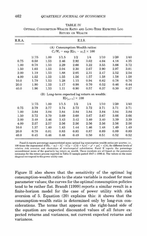
To interpret the patterns in Panel A of Table IV, consider first the right-hand column of the panel. This gives the exponentiated mean optimal log consumption-wealth ratio for an individual who is extremely reluctant to substitute consumption intertemporally (4' = o4o, close to zero). Such an individual wishes to maintain a constant expected consumption growth rate regardless of current investment opportunities. She can do this by consuming the long-run average return on her portfolio, with a precautionary- savings adjustment for risk. But in our model both the risk and the average return are endogenous. If the investor is highly risk-averse, as she is at the bottom of the column (-y = 40), then she holds almost all her wealth in the riskless asset and earns a low return with little risk; if she is close to risk-neutral, as she is at the top of the column (y = 0.75), she borrows at the riskless interest rate to earn a high but risky leveraged return. This explains why the mean consumption-wealth ratio is so much higher at the top of the column than at the bottom.

To clarify this interpretation, Panel B in Table IV reports the unconditional mean log portfolio return, E[rpt+i].18 The mean log returns in the right-hand column are close to the optimal consumption-wealth ratios given in the right-hand column of the upper panel (Panel A). They are particularly close at high levels of risk aversion, shown at the bottom of the tables; at the top of the panels the two variables diverge because the mean log return reaches a maximum when the coefficient of relative risk aversion y = 1, and starts to fall when risk aversion declines from this level, whereas the optimal consumption-wealth ratio keeps on rising as y falls below one. The investor with unit risk aversion maximizes the conditional expectation of the log portfolio return; hence this investor must also have the highest unconditional expected log portfolio return. The increase in the average consumption-wealth ratio as y falls below one is caused by the precaution-

18. We can compute the long-term or unconditional expected log return on wealth by taking unconditional expectations in Lemma 4 of Appendix 1, i.e., by calculating E[Et(rpt+ )], which gives

E[rpt+,] = rf + PO + PlEXt + p2E4t

= rf + po + Ply + P2(Ux2 + i2),

where po, p1, and P2 are functions of ao and a1 defined in Lemma 4. We can rewrite Po, P1, andp2 as functions of the normalized parameters a* and a1 by noticing that

ao - al((ou/2).


ary savings effect, which turns negative when ip and y are on the same side of unity as shown in equation (13).

Now consider what happens as the individual becomes more willing to substitute intertemporally; that is, as ip increases and we move to the left in Panel A of the table. Equation (20) helps us understand this. If we hold fixed the variance terms in (20), the derivative of ct - wt with respect to ip is -[p/(1 - p)](Et[(1 - p)/p]

1j'71 pJrp t~j + log 8), which is negative if the long-run expected portfolio return exceeds the rate of time preference and positive otherwise. Ignoring precautionary savings effects, an individual who is willing to substitute intertemporally will have higher saving and lower current consumption than an individual who is unwilling to substitute intertemporally if the time-preference- adjusted rate of return on saving is positive, but will have lower saving and higher current consumption if the adjusted return on saving is negative. Panel A in Table IV illustrates this pattern. Investors with low risk aversion y at the top of the table choose portfolios with high average returns, so a higher elasticity of intertemporal substitution ip corresponds to a lower average consumption-wealth ratio. Highly risk-averse investors at the bottom of the table choose safe portfolios with low average returns, so for these investors a higher ip corresponds to a higher average consumption-wealth ratio.

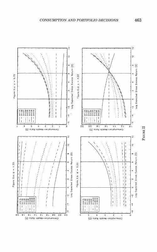
Our discussion so far has concentrated on the average level of consumption in relation to wealth. We now give some intuition about the sensitivity of the optimal ratio to the state variable xt. Although we have noted that the slope of the optimal consumption policy is always small in absolute value relative to the intercept, Figure II shows that around the mean of the state space it is negative when ip > 1, and positive when ip < 1. Moreover, it increases in absolute value as y decreases. The intertemporal substitution effect and the portfolio composition effect explain this pattern. As xt increases in the neighborhood of its positive mean, so does the expected return on wealth, causing income and substitution effects on consumption. When ii > 1, the substitution effect dominates, and the investor will cut consumption to exploit favorable investment opportunities. When 4i < 1, the income effect dominates, and the investor will increase consumption because a given quantity of wealth can sustain a greater flow of consumption. The effect of risk aversion appears because the state variable xt increases only the expected return on the risky asset, not the expected return on the riskless asset. An investor with a low risk


TABLE V VOLATILITY OF CONSUMPTION GROWTH AND VOLATILITY OF THE LOG

CONSUMPTION-WEALTH RATIO

R.R.A. E.I.S.

(A) Volatility of consumption growth: u(Act+l - EJ[A Ct+1]) X 100

11.75 1.00 1/1.5 1/2 1/4 1/10 1/20 1/40 0.75 37.12 31.17 27.41 26.12 24.71 24.13 23.97 23.90 1.00 33.44 27.47 23.49 22.08 20.55 19.91 19.74 19.66 1.50 27.43 22.32 18.63 17.28 15.83 15.26 15.11 15.05 2.00 23.07 18.84 15.62 14.41 13.12 12.65 12.54 12.49 4.00 13.93 11.63 9.69 8.93 8.16 7.95 7.92 7.92

10.0 6.31 5.42 4.61 4.29 3.99 3.97 4.00 4.02 20.0 3.29 2.87 2.47 2.31 2.17 2.19 2.21 2.22 40.0 1.68 1.48 1.28 1.20 1.14 1.15 1.17 1.18

(B) Volatility of the consumption-wealth ratio: (T(Ct+l - Wt+l - Et[ct+l - w t+1]) X 100

1/.75 1.00 1/1.5 1/2- 1/4 1/10 1/20 1/40 0.75 8.97 0.00 6.72 9.49 13.12 15.02 15.61 15.90 1.00 7.77 0.00 6.07 8.65 12.03 13.86 14.43 14.71 1.50 6.11 0.00 5.13 7.38 10.47 12.15 12.69 12.95 2.00 5.04 0.00 4.45 6.48 9.30 10.90 11.41 11.67 4.00 2.94 0.00 2.92 4.38 6.55 7.85 8.28 8.49

10.0 1.30 0.00 1.44 2.22 3.46 4.27 4.55 4.69 20.0 0.67 0.00 0.78 1.22 1.94 2.41 2.58 2.66 40.0 0.34 0.00 0.41 0.64 1.03 1.28 1.38 1.42

Panel A reports the percentage unconditional standard deviation of quarterly log consumption innovations for different levels of relative risk aversion and elasticities of intertemporal substitution, while Panel B reports the percentage unconditional standard deviation of innovations in the quarterly log consumption- wealth ratio. These numbers are all based on the parameter estimates for the return process reported in Table II (sample period 1947:1-1995:4). The values on the main diagonal correspond to the power utility case.

aversion coefficient is more heavily invested in the risky asset, and thus her expected portfolio return is more sensitive to changes in xt.

Finally, we consider the implications of the consumption rule for the volatility of consumption relative to past expectations and relative to wealth. Panel A in Table V reports the unconditional standard deviation of consumption innovations for each set of preferences we have considered, and Panel B reports the unconditional standard deviation of innovations in the log consumption- wealth ratio.

Panel A in Table V shows that investors with low risk aversion have extremely volatile consumption growth, for their


consumption inherits the volatility of their portfolios. Investors with unit elasticity of substitution in consumption have constant consumption-wealth ratios, and so their consumption volatility equals their portfolio volatility. Investors with low elasticity of intertemporal substitution have somewhat less volatile consumption, because they react to mean-reversion in stock returns by cutting their consumption-wealth ratios when the stock market rises. A 1 percent innovation in wealth causes these investors to increase consumption by less than 1 percent; they know that a 1 percent increase in consumption could not be sustained, even with 1 percent greater wealth, because the increase in wealth is accompanied by a decrease in expected portfolio returns. Inves- tors with high elasticity of intertemporal substitution respond to the decrease in expected returns by cutting saving, so their consumption is more volatile than their portfolio returns. Similar results are reported by Campbell [1996] for a model with an exogenous portfolio return process.

Panel B in Table V shows that investors with elasticities of intertemporal substitution different from one have volatile consumption-wealth ratios, because they do not consume a fixed fraction of their wealth each period, but a varying fraction that changes with the expected excess return on the risky asset. The volatility of the consumption-wealth ratio is increasing in the distance of the elasticity of intertemporal substitution from one, and is decreasing in risk aversion since less risk-averse investors have riskier portfolios whose expected returns are more sensitive to changes in investment opportunities.

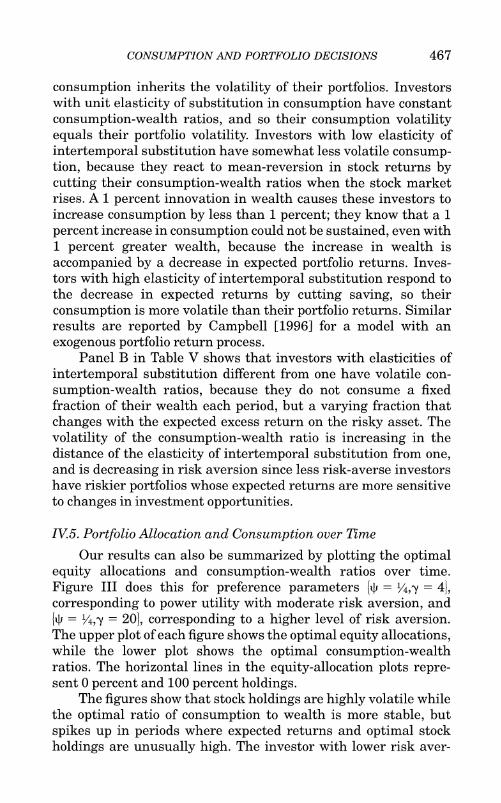
1V5. Portfolio Allocation and Consumption over Time

Our results can also be summarized by plotting the optimal equity allocations and consumption-wealth ratios over time. Figure III does this for preference parameters 1+ = V4,w = 41, corresponding to power utility with moderate risk aversion, and i+ = 4,-y = 201, corresponding to a higher level of risk aversion. The upper plot of each figure shows the optimal equity allocations, while the lower plot shows the optimal consumption-wealth ratios. The horizontal lines in the equity-allocation plots represent 0 percent and 100 percent holdings.

The figures show that stock holdings are highly volatile while the optimal ratio of consumption to wealth is more stable, but spikes up in periods where expected returns and optimal stock holdings are unusually high. The investor with lower risk aver-


0 ~~~~0

C - ~~~~~~~~~~~0 0

0/

IN

c)~~~~~~~

Ln ~ ~ ~~ 969

00'00000000000101 0 0' 0 0'90 00 9 10 0 91 0 90 0

(zcno~o o~o~ z)oo 110-Olwso


sion holds on average a much larger proportion of her wealth in stocks, and her consumption-wealth ratio is also larger on average and more volatile. But both investors are keen stock-market participants. In our model investors do not face restrictions on short sales, so we allow the optimal allocation to stocks to be either larger than 100 percent or negative. Figure III shows that in the U. S. postwar period both investors are long in stocks almost always, and the less risk-averse investor usually wants to short the riskless asset and invest more than 100 percent of her wealth in the market, except in periods of unusually low dividend yields such as the early 1970s and the mid-1990s.

Barberis [1999] has obtained similar results for a Bayesian investor who maximizes power utility defined over terminal wealth and uses the log dividend-price ratio as a state variable; with a ten-year investment horizon and access to historical data over the period 1927-1993, Barberis' investor, who is not allowed to short assets, is mostly 100 percent invested in stocks. Brennan, Schwartz, and Lagnado [1997] have studied a similar problem with power utility of terminal wealth, three state variables, three assets, and frequent portfolio rebalancing. They also do not allow short sales, and their optimal strategy for the period 1972-1992 often switches between 100 percent cash and 100 percent stocks. Their optimal strategy is more volatile than Barberis' or ours because they allow for a larger number of state variables. Brennan, Schwartz, and Lagnado also include long-term bonds in their analysis, but bonds do not play a major role in the optimal portfolio.

IV6. The Accuracy of the Solution

The analytical solutions we present in this paper are exact only in the limit where time is continuous, and for parameter values that imply a constant consumption-wealth ratio (+ = 1 or constant expected returns). For other parameter values our solutions are only approximate. One way to assess their accuracy is to compare them with solutions obtained using standard numerical methods.

In Campbell, Cocco, Gomes, Maenhout, and Viceira [1998], we have solved numerically for optimal policy functions in the calibrated model of this paper. The numerical solution discretizes the state space and approximates the distribution for the innovations in the random variables using Gaussian quadrature with nine quadrature points. The numerical method assumes that the


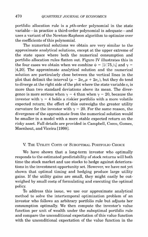
portfolio allocation rule is a pth-order polynomial in the state variable-in practice a third-order polynomial is adequate-and uses a variant of the Newton-Raphson algorithm to optimize over the coefficients of this polynomial.

The numerical solutions we obtain are very similar to the approximate analytical solutions, except at the upper extreme of the state space where both the numerical consumption and portfolio allocation rules flatten out. Figure IV illustrates this in the four cases we obtain when we combine + = 11/75,1,41 and -y = {4,201. The approximate analytical solution and the numerical solution are particularly close between the vertical lines in the plot that delimit the interval (,u - 2ux,,u + 2u,), but they do tend to diverge at the right side of the plot where the state variable xt is more than two standard deviations above its mean. The divergence is more serious when -y = 4 than when By = 20, because the investor with By = 4 holds a riskier portfolio with a more volatile expected return; the effect of this- outweighs the greater utility curvature for the investor with By = 20. For the same reason, the divergence of the approximate from the numerical solution would be smaller in a model with a more stable expected return on the risky asset. Full details are provided in Campbell, Cocco, Gomes, Maenhout, and Viceira [1998].

V. THE UTILITY COSTS OF SUBOPTIMAL PORTFOLIO CHOICE

We have shown that a long-term investor who optimally responds to the estimated predictability of stock returns will both time the stock market and use stocks to hedge against deteriora- tions in the investment opportunity set. However, we have not yet shown that optimal timing and hedging produce large utility gains. If the utility gains are small, they might easily be out- weighed by small costs of formulating and executing the optimal policy.

To address this issue, we use our approximate analytical method to solve the intertemporal optimization problem of an investor who follows an arbitrary portfolio rule but adjusts her consumption optimally. We then compute the investor's value function per unit of wealth under the suboptimal portfolio rule and compare the unconditional expectation of this value function with the unconditional expectation of the value function in the


/ N

/ ~~~~~~~~~00~

0~~~~~~~~~~

o 0

I 0

I I i

_______________________________~~~Lr I n __ _ _ __ _ _ _ __ _ _ _ __ _ _ I 009 O~~~t' 00S 00~~~ 001 0 Oat- 00~~~~~- 00c0' 0n0~ ~ 0- 0~

(4 s~~po~ o~~ uoi~o~o~~ (4 S~l~~O~S O~ U~~i4O~OIIV


unrestricted problem.19 Throughout we assume that the investor knows the stochastic process driving the return on the risky asset; that is, we ignore the parameter uncertainty addressed by Kandel and Stambaugh [1996] and Barberis [1999].

We consider three restricted portfolio rules. The first rule ignores the timing implied by the optimal portfolio policy and sets the equity allocation each period to the average allocation under the optimal rule. This is a fixed portfolio rule that allows for partial hedging in the spirit of the investment strategy advocated by Siegel [1994]. Siegel argues that long-run investors should not try to time the stock market, but should buy and hold large equity positions because these positions involve little risk at long horizons. Siegel's estimates of long-run stock market risk are low because of the mean-reversion in stock returns that we have captured with our VAR system. Thus, one can interpret Siegel's strategy as a hedging strategy without market timing. The second portfolio rule is the myopic rule that times the market but ignores hedging considerations. This rule would be optimal if the covariance u-quwere zero. The third rule sets the equity allocation each period to the average allocation under the myopic rule, ignoring both timing and hedging considerations.

Table VI describes the optimal consumption rules implied by the restricted portfolio rules. For comparison it also includes in its first row the optimal consumption rule (27) under the optimal portfolio rule (26). The parameters of these rules of course depend on the exogenous parameters of the model, but to save space, we do not give further details here.

The top left panel of Table VII reports the unconditional mean of the value function per unit of wealth that is implied by the optimal, unrestricted consumption and portfolio rules in the calibrated example discussed in the previous section. The other three panels report the percentage change in the value function when portfolio choice is restricted to one of the suboptimal rules described above.

The table shows that suboptimal portfolio choice can cause large losses in utility. Failing to hedge intertemporally is harm- less when risk aversion My = 1, since in this case the optimal portfolio is myopic, but it can be a serious error for investors with My > 1. The losses from failing to hedge increase at first as risk

19. The implied value functions are exponentials of quadratic or linear functions of the state variable. The results in Constantinides [1992] allow us to obtain explicit formulas for their unconditional expectations.


TABLE VI OPTIMAL CONSUMPTION RULES IMPLIED BY RESTRICTED PORTFOLIO RULES

Portfolio rule Optimal consumption rule given portfolio rule

Hedging

Timing at = ao + al(xt + u /2) ct - wt b* + b*(xt + ur/2) + b2(xt + U2/2)

No-timing at = a* + al(y + U2 /2) c t - wt b hnt + bhit (xt + U2/2)

No-hedging

Timing xt + (X2/2 ct - Wt = brit + b nh t(xt + U(2/2)

at =

2 + bilit (xt + (2 /2)

No-Timing Y + (X2/2 ct - Wt = bihnt + b nhtnt(xt + (Y2/2) at = 2

-y(t

The second column in Table VI describes the consumption rule followed by an investor who adjusts consumption optimally given the portfolio rule described in the first column of the table. The first row describes the optimal consumption rule implied by the unconstrained optimal portfolio rule. This rule is state-dependent and includes a hedging component. Therefore, the first row of the table describes the solution to the intertemporal optimization problem we solve in Section III. The second row describes the optimal consumption rule followed by an investor who follows a suboptimal portfolio rule consisting in allocating to stocks each period a fixed fraction of her savings that equals the average allocation to stocks implied by the optimal portfolio rule. Therefore, this investor ignores timing in her portfolio decisions, though she allows for (imperfect) hedging. The third row of the table describes the optimal consumption rule followed by an investor who follows a myopic portfolio rule. This suboptimal portfolio rule ignores hedging, but it is time-dependent. Finally, the fourth row of the table describes the optimal portfolio rule followed by an investor who ignores both hedging and timing and invests in stocks each period a fixed fraction of her savings that equals the average myopic allocation to stocks.

aversion increases above one, but eventually diminish as extremely risk-averse investors have only very small equity positions and thus have little to hedge. Failing to time the market causes large losses for all investors except those who are extremely risk-averse but extremely willing to substitute consumption intertemporally. For all parameter values we consider, the failure to time the market causes larger utility losses than the failure to hedge intertemporally. These results confirm, for a variety of investors with different levels of risk aversion and elasticity of intertemporal substitution, the findings of Balduzzi and Lynch [1997b] for finite-horizon investors with isoelastic preferences defined over wealth and relative risk aversion coefficients of 2, 6, and 10.20 The results are also compatible with the

20. Balduzzi and Lynch find that utility losses increase with the horizon of the investor. Since we consider an infinite horizon, this helps to explain why we obtain somewhat larger utility costs than they do for similar levels of risk aversion. Balduzzi and Lynch also find that utility costs remain substantial in the presence of fixed and proportional transaction costs.


findings of Kandel and Stambaugh [1996] and Barberis [1999] that Bayesian investors experience large gains in certainty- equivalent return when they optimally respond to evidence of predictability in stock returns.

VI. CONCLUSION

One of the major objectives of modern financial economics has been to put investment advice on a scientific basis. This task has been accomplished for investors who have short horizons or constant investment opportunities. Unfortunately, most investors have long horizons, and there is considerable evidence that they face time-varying expected returns on risky assets. Until very recently financial economists have not even attempted to give such investors precise quantitative advice about their portfolio strategies.

Recent work on long-horizon portfolio choice has generally ignored the consumption decision and has considered portfolio choice for investors who consume nothing until a fixed terminal date.21 Our objective has been to analyze a model in which investors optimize over both consumption and portfolio allocation. Because the intertemporal consumption and portfolio choice problem is highly intractable when expected returns are time varying, we have resorted to an analytical approximation. We have replaced the Euler equations and budget constraint of the exact problem with approximate equations that are much easier to solve, and we have explored in detail the analytical solution of the approximate problem.

We have used Epstein-Zin-Weil recursive preferences to separate the influence of risk aversion and the elasticity of intertemporal substitution on portfolio choice and consumption. We have shown, for example, that portfolio choice depends on the elasticity of intertemporal substitution only indirectly through the effect of this elasticity on the average level of consumption relative to wealth.

We have used our model to assess the quantitative impor- tance of intertemporal hedging demand for risky assets by long-lived investors. After calibrating the model to postwar quarterly U. S. stock market data, we find that intertemporal hedging

21. Very recent exceptions to this statement include Brandt [1999] and some cases analyzed in Balduzzi and Lynch [1997a,1997b].


motives can easily double the average total demand for stocks by investors whose coefficients of relative risk aversion exceed one. We also find that suboptimal myopic portfolio rules imply large utility losses for such investors. These results support the conclusion of other recent papers such as Barberis [1999], Balduzzi and Lynch [1997a, 1997b], Brandt [1999], Brennan, Schwartz, and Lagnado [1997], and Kim and Omberg [1996] that static models of portfolio choice can be seriously misleading. Intertemporal portfolio choice should not remain an abstruse theoretical topic, but should be integrated into empirical research and investment practice.

An important caveat is that our analysis is partial equilibrium in nature. We solve the macroeconomic problem of a given investor facing exogenous asset returns, but we do not show how these asset returns could be consistent with general equilibrium. One possibility is that the representative investor has different preferences from those assumed here, perhaps the habit- formation preferences of Campbell and Cochrane [1999] that can generate shifts in risk aversion and hence changing risk premiums with a constant riskless interest rate. In this setting the model has only limited applicability, since it describes the behavior of atypical investors whose risk aversion is constant over time. Alternatively, if all investors have the preferences assumed here, their portfolio shifts could be supported in general equilibrium by shifting asset supplies. Supplies of stock would have to fall with the risk premium to accommodate investors' desire to reduce their stockholdings. But such shifts in supplies are unlikely to be consistent with macroeconomic data on aggregate portfolio shares.

Another caveat has to do with approximation error. Our approximate solution is exact when the elasticity of intertemporal substitution is one and the time interval between consumption and portfolio decisions is infinitesimally small. In a companion paper [Campbell, Cocco, Gomes, Maenhout, and Viceira 1998] we have checked the accuracy of the analytical approximate solution in other cases by comparing it with a discrete-state numerical solution in our calibrated example. We have found that our solution is generally a good approximation to the true solution, but the approximation error does increase when the state variable is more than two standard deviations above its mean. We have also found that the numerical solution algorithm converges much more rapidly and reliably when we are able to provide starting values from the approximate solution.


and

rpt+l - Etrp,t+l (aO + alxt)ut+i,

where

Go= aO(I - ao)(u 2z/2). Po It-(1 --

P1= ao + al(l - 2ao)(C2/2)

P2 = a - a,( u/2).

Proof of Lemma 4. From (16) and our guess (i) on the optimal portfolio rule, we have that

Etrpt+l = ultEt[rj't+j - rf] + rf + (o2 /2)tt(l - at)

= (aO + alxt)xt + rf + (u2/2)((ao + alit) - (aO + alxt)2),

where the last line follows from (2). Reordering terms, we get a quadratic expression in xt whose coefficients are those given in the statement of the proposition.

The expression for rpt+1 - Etrpt+l also follows from (16) and guess (i), as well as (Al)-constant rf -and (A2)-(2),

(29) rpt+l - Etrp,t+l = xt((rj,t+j - rf) - Et[rl,t+l - rf])

= (aO + alxt)ut+i.

EL

LEMMA 5. Expected optimal consumption growth over the next period is quadratic in the current state variable, and unexpected consumption growth is linear in the current state variable:

EtAct+l = Etrpt+l + Et[ct+l - wt+]- - (ct - wt) + k

= Co + clxt + C2Xt,

Act+i - EtAct+l = (aO + aixt)ut+l + blqt+l

+ b2(2u(1 - I) + 2+xt),qt+j + b2(,t2q1 - (T),


where

2 co = rf + ao(l - ao) 2 + k + bo 1 - -h + bl(y(l - )

+ b2(j2(1 - 4)2 + U2) 2 I1\~~2

cl ao + al(1 - 2aO) 2 + b - + b2(21z(1-l 2 pj

a,1- a2 - + b2(+2 - -)

Proof of Lemma 5. From (18) and (15) we can write

(30) Act+, = rpt+l + (ct+l - wt+i) - (1/p)(ct - wt) + k.

Therefore,

EtAct+l = Etrp,t+l + Et(ct+l - wt+i) - - (ct - wt) + k p

= Po + PlXt + p2Xt2 rf

+ b(1 ) Etxt+ - -xt + b - + k

= ao(l - ao) 2 + (ao + a - aoal(u)xt + a,(1 - a 2)Xt

+ rf + b0(o 1 p + bi[u(1 - 4) + -

+ b4[t2(1 - 4)2 + U2 + 2yu4(1 - 4)xt + (22 - + k,

where the second equality follows from Lemma 4 and our guess (ii) on the optimal consumption policy, and the last equality follows from (3) and Lemmas 1 and 2. Reordering terms, we get the expression for Etlct+l in the lemma as well as Ico,c1,c22.

The expression for unexpected consumption growth follows from (30), the expression for the unexpected portfolio return derived in Lemma 4, and from noting that our guess (ii) on the


Proof of Lemma 6. From (13), (15), and (18) we have

1 p t= - ( vart (A-ct+i - 4arpt+i)

1 - _ Et[(ct+l - EtAct+) - (rpt+l -Etrpt+l)]2

1 0 - _() Et[(1 - 4j)(rpt+l - Etrpt+i)

+ (ct+l - wt+i) - Et(ct+l - Wt+,)]2.

If we substitute in the bracketed expression above (29) and (31) for (rpt+l - Etrpt+i) and (ct+1 - wt+i) - Et(ct+l - wt+i) and compute Et under assumptions (A2) and (A3), we find that vp t is a quadratic function of xt, with the coefficients given in the statement of the lemma. EZ

LEMMA 7. The parameters defining the optimal consumption rule (ii) satisfy the following three-equation system:

2

O= k - t log 8 + (1 - lj)rf + (1 - l)ao(1 - ao) 2

1~~~~~~~~~

+ bo1 -- + bl(jt(l - 4)) + b2(j2(1 - 4)2 + U2)

V1 =ao(1 - 4') + (1 - t')aj(l - 2ao) 2U + bl(4 - )

+ b2(2jt+(1 -

v2=al(l -4')- (1 - q)a2l + b2(42 \) Proof of Lemma 7. This follows from the log-linearized Euler

equation for the optimal portfolio given in (12), and Lemmas 4, 5,


LEMMA 9. The covariance between unexpected stock returns and changes in the expected value of the intercept in the Euler equation (13) is linear in the state variable:

covt (rlt+l - Etrl,t+i,(Et+l - Et)I piv,,t+j = ((v1 + 2V2j) 1

- 2v2 1-

+ 2V21 _ p Uqu xt,

where {vo,v1,v2} are given in Lemma 6.

Proof ofLemma 9. Lemma 6 implies that

(Et+, - Et) E pivp~t+j = v1E pi(E t+1 - Et)xt+j j=l j=l

+ V2 I pi(E t+1 - Et t+j7 j=1

which is identical to the expression given in the proof of Lemma 8, except that we have v1 and v2 instead of p1 and P2. Therefore, we must have that

(Et+, - Et) I pjvpt+ i = Vi1 + 2V2(Xt - j)

+2V2Y 1 t+l

P 2 P 2 + V2 -p(2T nt+1-V2 p(V V

from which the lemma follows, under the distributional assumptions (A2) and (A3). E


+ [-B21A11 - B22 + (V22 - B25)AjjA2O + V24A20]b1

+ [-B21A12 - B23 + (V22 - B25)(AlOA21 + A12A20)

+ V23A10 + V25A20- B24A2-1b2

+ [V21 + (V22 - B25)A12A21 + V23A12 + V25A21]b2

+[(V22 - B25)AjjA21 + V23A11 + V24A21 + V26]blb2,

0 = (V31 - B33)A20 - B31A

+ [2(V31 -B33)A20A2

- B31A21 - B32 + V33A20]b2

+ [(V31 - B33)A21 + V32+ V33A21]b2. D

APPENDIX 3: PROOFS OF PROPERTIES

Proof of Property 1

The approximate value function per unit of wealth obtains by direct substitution of guess (ii) into (11). We now use equation (23) to characterize b2. This equation is

0 = A30 + A31b2+ A32b22

Substituting Aij's for their values, we get

(35) 0= 2 - [l 2 )4 + --b2

[2(1 - y)4+2[U21)U - 2 2

This equation has two roots, that we denote 1b21,b22}. A sufficient (but not necessary) condition for these roots to be real is that

A32A30 '

0;

i.e.,

(1-)(2[ffy2 + *0-(U 2-(T u)]

2U4 'y o-

This is always true when -y 1, since (1 - y) ' 0;

(36) 2U 2

2U = U 2 u2(1 - corr (u )2) 2

0;


Substituting y = 1 in Proposition 1, we obtain the same myopic portfolio rule as with log utility. It is straightforward to see that this rule maximizes the conditional expectation of the log portfolio return. However, the consumption-wealth ratio is no longer constant unless t = 1, as we can see from Lemma 7 in Appendix 1. Therefore, unit relative risk aversion implies a myopic optimal portfolio policy and a nonmyopic optimal consumption policy. Giovannini and Weil [1989] emphasize this result. D

Part b. When 4i - 1, the equation system in Proposition 2 delivers b1 = b2 =0 and

bo = (p/(l - p))(k - log 6).

After substituting for the value of k, this result simplifies to

(40) bo = log (1 - p).

Moreover, we know from standard arguments that p = 6. There- fore, it is optimal for the individual to consume each period a fixed fraction of her wealth. Following Giovannini and Weil [1989], we call this optimally constant propensity to consume out of wealth a myopic consumption policy.

However, the agent's optimal portfolio policy is not myopic. This is because, from equation (41) in the proof of Property 3 below, we have that b2/(1 - 4i) and b1/(l - 4i) are nonzero constants independent of 4i for given p. Therefore, when i = 1, the terms in 1b1,b2l in the system defining the optimal portfolio policy in Proposition 1 do not vanish, and a nonmyopic portfolio policy obtains. Giovannini and Weil [1989] also emphasize this result.

Part c. The values for bo, bl, and b2 obtain from the proof for Part b. Substituting fory = 1 into Proposition 1, we obtain ao = 0 2 and a, 1/u. D

Part d. With constant expected returns, uqu = 0. From Proposition 1 we obtain the same portfolio policy as in the log utility case, except that -y # 1: a0 = 1/(2y), and a, = 1/yu2. Also, since xt is deterministic, (31) implies that ct - wt is constant. This is the well-known result for the optimal portfolio rule when returns are i.i.d. D

Proof of Property 4

A straightforward analysis of the solutions to equations (22) and (23) in Proposition 2 shows that we can write b1 and


b2as

b 1 = (+- 1)f(-y,p),

(41) b2 = 1)f2(-y,p),

where f1(y,p) and f1(y,p) are functions that do not depend on 4. After substitution in the equation system in Proposition 1, we find that the parameters defining the optimal portfolio rule, Iao,al}, do not depend on 4i for given p. However, p itself is a function of 4i-recall that p = 1 - exp IE[ct - wt]}-so the optimal portfolio rule depends on q indirectly through p. D

Proof of Property 5

To prove this result, note that equation (23) in Proposition 2, that determines b2, is found by equating the right-hand side of the third equation in Lemmas 6 and 7, and substituting out a, using the second equation in Proposition 1. None of these equations depend on jt. F

HARVARD UNIVERSITY AND NATIONAL BUREAU OF ECONOMIC RESEARCH HARVARD UNIVERSITY

REFERENCES

Balduzzi, Perluigi, and Anthony Lynch, "The Impact of Predictability and Transac- tion Costs on Portfolio Choice in a Multiperiod Setting," unpublished paper, Boston College and New York University, 1997a.

Balduzzi, Perluigi, and Anthony Lynch, "Transaction Costs and Predictability: Some Utility Cost Calculations," unpublished paper, Boston College and New York University, 1997b.

Barberis, Nicholas C., "Investing for the Long Run When Returns Are Predictable," Journal of Finance, LIV (1999), forthcoming.

Brandt, Michael W., "Estimating Portfolio and Consumption Choice: A Conditional Euler Equations Approach," Journal of Finance, LIV (1999), forthcoming.

Brennan, Michael J., Eduardo S. Schwartz, and Ronald Lagnado, "Strategic Asset Allocation," Journal of Economic Dynamics and Control, XXI (1997), 1377- 1403.

Campbell, John Y., "Stock Returns and the Term Structure," Journal of Financial Economics, XVIII (1987), 373-399. , "Intertemporal Asset Pricing without Consumption Data," American Eco- nomic Review, LXXXIII (1993), 487-512. , "Understanding Risk and Return," Journal of Political Economy, CIV (1996), 298-345.

Campbell, John Y., and John H. Cochrane, "By Force of Habit: A Consumption- Based Explanation of Aggregate Stock Market Behavior," Journal of Political Economy, CVII (1999), 205-251.

Campbell, JohnY., Jodo Cocco, Francisco Gomes, Pascal J. Maenhout, and Luis M. Viceira, "Stock Market Mean Reversion and the Optimal Equity Allocation of a Long-Lived Investor," unpublished paper, Harvard University, 1998.


Campbell, John Y., and Hyeng Keun Koo, "A Comparison of Numerical and Analytical Approximate Solutions to an Intertemporal Consumption Choice Problem," Journal of Economic Dynamics and Control, XXI (1997), 273-295.

Campbell, John Y., Andrew W. Lo, and A. Craig MacKinlay, The Econometrics of Financial Markets (Princeton, NJ: Princeton University Press, 1997).

Campbell, John Y., and N. Gregory Mankiw, "Consumption, Income, and Interest Rates: Reinterpreting the Time-Series Evidence," in NBER Macroeconomics Annual 1989 (Cambridge, MA: MIT Press, 1989).

Campbell, John Y., and Robert Shiller, "The Dividend-Price Ratio and Expecta- tions of Future Dividends and Discount Factors," Review of Financial Studies, I (1988a), 195-227.

Campbell, John Y., and Robert Shiller, "Stock Prices, Earnings, and Expected Dividends," Journal of Finance, XLIII (1988b), 661-676.

Campbell, John Y., and Luis M. Viceira, "Consumption and Portfolio Decisions When Expected Returns Are Time Varying," NBER Working Paper No. 5857, 1996.

Campbell, John Y, and Luis M. Viceira, "Who Should Buy Long-Term Bonds?" NBER Working paper No. 6801, 1998.

Cecchetti, Steven, Pok-sang Lam, and Nelson C. Mark, "Testing Volatility Restric- tions on Intertemporal Marginal Rates of Substitution Implied by Euler Equations and Asset Returns," Journal of Finance, XLIX (1990), 123-152.

Cochrane, John, and Lars P. Hansen, "Asset Pricing Explorations for Macroeconom- ics," in NBER Macroeconomics Annual 1992 (Cambridge, MA: MIT Press, 1992).

Constantinides, George M., "A Theory of the Nominal Term Structure of Interest Rates," Review of Financial Studies, V-(1992), 531-552.

Cox, John C., and Chi-fu Huang, "Optimal Consumption and Portfolio Policies When Asset Prices Follow a Diffusion Process," Journal of Economic Theory, XXXIX (1989),33-83.

Duffie, Darrell, and Lawrence Epstein, "Stochastic Differential Utility," Economet- rica, LX (1992), 353-394.

Elliott, Graham, and James H. Stock, "Inference in Time Series Regression When the Order of Integration of a Regressor Is Unknown," Economic Theory, X (1994), 672-700.

Epstein, Lawrence, and Stanley Zin, "Substitution, Risk Aversion, and the Temporal Behavior of Consumption and Asset Returns: A Theoretical Frame- work," Econometrica, LVII (1989), 937-969.

Epstein, Lawrence, and Stanley Zin, "Substitution, Risk Aversion, and the Temporal Behavior of Consumption and Asset Returns: An Empirical Investi- gation," Journal of Political Economy, XCIX (1991), 263-286.

Fama, Eugene, and Kenneth French, "Dividend Yields and Expected Stock Returns," Journal of Financial Economics, XXII (1988), 3-27.

Fama, Eugene, and Kenneth French, "Business Conditions and Expected Returns on Stocks and Bonds," Journal of Financial Economics, XXV (1989), 23-49.

Fischer, Stanley, "Investing for the Short and the Long Term," in Zvi Bodie and John B. Shoven, eds., Financial Aspects of the United States Pension System (Chicago, IL: The University of Chicago Press, 1983).

Giovannini, Alberto, and Philippe Weil, "Risk Aversion and Intertemporal Substi- tution in the Capital Asset Pricing Model," NBER Working Paper No. 2824, 1989.

Goldman, M. Barry, "Anti-Diversification or Optimal Programmes for Infrequently Revised Portfolios," Journal of Finance, XXXIV (1979), 505-516.

Hall, Robert E., "Intertemporal Substitution in Consumption," Journal of Political Economy, XCVI (1988),339-357.

Hamilton, James D., Time Series Analysis (Princeton, NJ: Princeton University Press, 1994).

Hansen, Lars P., and Ravi Jagannathan, "Restrictions on Intertemporal Marginal Rates of Substitution Implied by Asset Returns," Journal of Political Economy, XCIX (1991), 225-262.

He, Hua, and Neil D. Pearson, "Consumption and Portfolio Policies with Incom- plete Markets and Short-Sale Constraints: The Infinite-Dimensional Case," Journal of Economic Theory, LIV (1991), 259-304.


Hodrick, Robert J., "Dividend Yields and Expected Stock Returns: Alternative Procedures for Inference and Measurement," Review of Financial Studies, V (1992), 357-386.

Ingersoll, Jonathan E., Jr., Theory of Financial Decision Making (Totowa, NJ: Rowman and Littlefield, 1987).

Kandel, Shmuel, and Robert Stambaugh, "On the Predictability of Stock Returns: An Asset Allocation Perspective," Journal of Finance, LI (1996), 385-424.

Kim, Tong Suk, and Edward Omberg, "Dynamic Nonmyopic Portfolio Behavior," Review of Financial Studies, IX (1996), 141-161.

Kocherlakota, Narayana R., "The Equity Premium: It's Still a Puzzle," Journal of Economic Literature, XXXIV (1996), 42-71.

Mehra, Rajnish, and Edward C. Prescott, "The Equity Premium: A Puzzle," Journal of Monetary Economics, XV (1985), 145-161.

Merton, Robert C., "Lifetime Portfolio Selection under Uncertainty: The Continu- ous Time Case," Review of Economics and Statistics, LI (1969), 247-257. , "Optimum Consumption and Portfolio Rules in a Continuous-Time Model," Journal of Economic Theory, III (1971), 373-413. , "An Intertemporal Capital Asset Pricing Model," Econometrica, XLI (1973), 867-887. ,Continuous Time Finance (Cambridge, MA: Basil Blackwell, 1990).

Restoy, Fernando, "Optimal Portfolio Policies under Time-Dependent Returns," Bank of Spain Working Paper 9207, Bank of Spain, Madrid, Spain, 1992.

Samuelson, Paul A., "Lifetime Portfolio Selection by Dynamic Stochastic Program- ming," Review of Economics and Statistics, LI (1969), 239-246.

Schroder, Mark, and Costis Skiadas, "Optimal Consumption and Portfolio Selection with Stochastic Differential Utility," Working Paper 226, Department of Finance, Kellogg Graduate School of Management, Northwestern University, 1998.

Siegel, Jeremy J., Stocks for the Long Run (Burr Ridge, IL: Richard D. Irwin, 1994).

Svensson, Lars E. O., "Portfolio Choice with Non-Expected Utility in Continuous Time," Economics Letters, XXX (1989), 313-317.

Viceira, Luis M., "Optimal Portfolio Choice for Long-Horizon Investors with Nontradable Income," unpublished paper, Harvard University, 1997.

Weil, Philippe, "The Equity Premium Puzzle and the Risk-Free Rate Puzzle," Journal of Monetary Economics, XXIV (1989), 401-421.

consumption and portfolio decisions when expected returns...

Documents