consumption and debt response to unanticipated income
TRANSCRIPT

1
Consumption and Debt Response to Unanticipated Income Shocks:
Evidence from a Natural Experiment in Singapore *
Sumit Agarwal
National University of Singapore, [email protected]
Wenlan Qian
National University of Singapore, [email protected]
September, 2013
Abstract
This paper uses a unique panel data set of consumer financial transactions to study how
consumers respond to an exogenous unanticipated income shock. We find that consumption rose
significantly subsequent to the fiscal policy announcement: for each dollar received, consumers
on average spent 90 cents during the ten months after the program’s announcement. There was a
moderate decrease in debt. We find a strong announcement effect—consumers increased
spending via their credit cards during the two-month announcement period, but they switched to
debit cards after disbursement, before finally increasing spending on the credit card in the later
months.
Keywords: Consumption, Spending, Debt, Credit Cards, Household Finance, Banks, Loans,
Durable Goods, Discretionary Spending, Fiscal Policy, Tax Rebates, Liquidity Constraints,
Credit Constraints.
JEL Classification: D12, D14, D91, E21, E51, E62, G21, H31
*Corresponding author: Wenlan Qian, 15 Kent Ridge Drive, NUS Business School, Singapore 119245, phone: (65)
65163015, email: [email protected]. We benefited from the comments of Chris Carroll, Souphala
Chomsisengphet, Steve Davis, Takeo Hoshi, Tullio Jappelli, David Laibson, Brigitte Madrian, Neale Mahoney, Jessica Pan, Ivan Png, Nagpurnanand Prabhala, Tarun Ramadorai, David Reeb, Amit Seru, Nick Souleles, Bernard
Yeung, and seminar participants at the World Bank, Oxford University, John Hopkins University, European
Conference on Household Finance, 7th
Singapore International Conference on Finance, Econometric Society Asian
Meeting, Asian Bureau of Finance and Economic Research Inaugural Meeting, Nanyang Technological University,
National University of Singapore. Funding from the NBER Household Finance Working Group through the Alfred P.
Sloan Foundation is gratefully acknowledged.

2
1. Introduction
A central implication of the life-cycle/permanent income hypothesis (LCPIH) is that consumers
should not respond to predictable and temporary changes in their income. Many studies, however,
have rejected the LCPIH, noting declines in spending across time after a temporary change to
income. Researchers have explained these declines across time primarily through liquidity
constraints and precautionary savings (see, Souleles 1999, Carroll 1992, Johnson, Parker, and
Souleles 2006, Agarwal, Liu, and Souleles 2007, Parker et al. 2013).
In this paper, we use a unique panel data set of consumer financial transactions to study how
consumers respond to an exogenous unanticipated income shock.1 Specifically, we use a
representative sample of more than 180,000 consumers in Singapore and study how their credit
card, debit card, and bank checking account spending behavior responded to a positive income
shock, the Growth Dividend Program announced by the Singapore government in February 2011.
The US$1.17 billion package distributed a one-time cash payout, ranging from US$78 to
US$702, to 2.5 million adult Singaporeans. The package is 0.5% of the annual GDP of
Singapore in 2011, which is comparable to the size of the 2001 and 2008 US tax rebate. This
payment represents a significant income bonus, corresponding to about 18 percent of monthly
median income in Singapore in 2011. Our analysis is based on a difference-in-differences
identification that exploits the program’s qualification criteria—foreigners did not qualify for the
program and thus comprise the control group in the study. In addition to allowing us to identify
the causal impact of the fiscal policy on consumption, the richness of our data also lets us study
the response in credit card spending and debit card spending, the change in credit card debt, and
the change in banking transaction behavior in the 10 months following the policy announcement
to help us understand different channels of the consumption response.
As discussed by Gross and Souleles (2002), credit cards play an important role in consumer
finances, so they can be quite useful for studying consumer spending behavior. Half of
consumers in the United States have a credit card, and total credit card debt was close to a trillion
dollars in 2012 with 40 percent of revolving debt (U.S. Census Bureau, Statistical Abstract of the
United States:2012). Consumer credit plays an equally important role in Singapore. More than a
third of consumers in the country have a credit card, and the total credit card debt as a percentage
of GDP was over 2 percent in Singapore in 2011 (Department of Statistics Singapore, 2012).
Hence, the ability of consumers to manage credit well has direct implications for the welfare
impact of consumer credit proliferation. However, Agarwal et al. (2007) point out the limitations
of studying consumption dynamics using only credit card data, because credit cards potentially
miss significant spending via other instruments (debit cards, cash, and checks).2 For example,
1Although our objective is not to test any specific theoretical model, our results can be interpreted as a test of the LCPI
model. If the LCPIH holds, we should not find significant increases in spending over a broad window after a
temporary and unexpected change in income. 2 However, it is important to point out that disposable consumption is likely to be spent on debt or via credit cards and
not by using checks or other instruments.

3
the purchase volume on debit cards was similar in magnitude to that on credit cards in the United
States in 2012 (2.1 trillion vs. 2.3 trillion U.S. dollars) (U.S. Census Bureau, Statistical Abstract
of the United States:2012). Similarly, in Singapore debit and credit cards are important mediums
of disposable consumption. Virtually, everybody in Singapore has a debit card. Close to 30
percent of aggregate personal consumption in the country is already being purchased using credit
and debit cards. The remaining 70 percent of consumption is transacted via checks, direct
transfers, and cash. This study focuses on debt dynamics of households brought on by income
changes and therefore we are particularly interested in credit card usage, because credit cards
represent the leading source of unsecured credit for most households.3
We estimate a distributed lag model using the announcement date of the Dividend Growth
Program as the exogenous event and observe the impulse response of credit card spending, debit
card spending, and debt. Our findings are summarized as follows. First, recipients’ consumption
rose significantly after the fiscal policy announcement: for each dollar received, consumers on
average spent 90 cents (aggregated across different financial accounts) during the ten months
after the announcement. At the same time, consumers’ credit card debt decreased moderately (so
savings effectively increased). Second, we find a strong announcement effect: consumers started
to increase spending during the two-month period after the announcement but before the cash
payout. The magnitude of the response during the announcement period is comparable to that
after disbusrment. The announcement effect is consistent with the life-cycle theory but
inconsistent with past empirical evidence (Poterba, 1988 and Wilcox, 1989). One reason the past
studies could not find any effect is because they had limited time series observations to pick up
any announcement effect or the announcement was not a surprise. Third, consumption response
was concentrated in debit card (25 percent of the total response) and credit card (75 percent of
the total response) spending. Based on Agarwal et al. (2007), we expect the consumption
response to show up in credit card spending. We find that consumers started spending via credit
cards during the announcement period, then switched to debit cards after disbursement, before
finally increasing their credit card use significantly. Consistent with Agarwal et al. (2007), credit
card debt dropped in the first months after disbursement and then reverted back to its original
level. Lastly, consumption response was heterogeneous across spending categories and across
individuals. Consumption rose primarily in the non-food, discretionary category. Liquidity
constrained consumers showed a strong consumption response, whether or not they were credit
constrained.
We conduct a series of robustness tests to ensure that our results are not confounded by other
policy changes in Singapore. For instance, during the sample period two other policy changes
provided positive income shocks that could have affected consumption—all low-income
Singaporeans and citizens above the age of 45 received these shocks. To be certain that these
policies were not confounding our study, we dropped low-income households from our analysis
3Japelli, Pischke, and Souleles (1998) found that people with bankcards were better able to smooth their consumption
past income fluctuations than were people without bankcards.

4
to isolate the consumption response to the Growth Dividend Program. The second policy
targeted older Singaporeans (age ≥ 45) by topping up their illiquid retirement medical accounts,
which can only be applied to hospitalization or certain out-patient care items and cannot be
cashed out. To further validate our results, we carried out a separate analysis on a subsample of
consumers younger than 45 years old who were entitled only to the Growth Dividend Program.
We also perform additional tests against other confounding events or alternative explanations.
The results from these robustness tests are qualitatively and quantitatively similar to those in the
main analysis.
A vast literature examines consumption responses to income shocks (e.g., Shapiro and Slemrod
1995, 2003a, 2003b, Souleles 1999, 2000, 2002, Parker 1999, Hsieh 2003, Stephens 2003, 2006,
2008, Johnson, Parker, and Souleles 2006, Parker et al. 2013). The literature finds mixed
evidence: some studies find that consumption response is essentially zero, while others find that
liquidity constrained consumers respond positively to fiscal stimulus programs. For a review of
the literature see Browning and Collado (2003), and Jappelli and Pistaferri (2010).
Our paper is most closely related to Agarwal et al. (2007). Both our study and theirs look at the
dynamics of consumption and debt as a function of an income shock. Like Agarwal et al., we find
a significant spending response working through the balance sheets of the consumers, and we
confirm that liquidity constraints matter. However, we document the dynamics of the consumption
response across different spending instruments—a rise in credit card spending following the
announcement, then a switch to debit card spending after disbursement of the stimulus, and finally,
a switch back to the credit card in the later months. These dynamics imply that Agarwal et al.
(2007) underestimate the spending response due to limitations in their data. Specifically, they are
unable to measure spending via debit cards, which we show accounts for a significant portion of
the marginal propensity to consume (MPC), especially in the initial months after disbursement.
We are also the first to document that the spending response of credit constrained consumers is
dominated by that of the liquidity constrained consumers. Existing literature finds that
consumption responds significantly to relaxation of the credit constraints (Gross and Souleles,
2002; Agarwal et al., 2007; Leth-Petersen, 2010). Our data allow us to differentiate liquidity
constraints and credit constraints, and we find that credit constrained but liquidity unconstrained
consumers do not respond to the stimulus, while liquidity constrained consumers with credit
capacity respond strongly both in spending and debt behavior. This implies that the MPC for the
liquidity constrained consumers, estimated from the prior studies, might be a lower bound of their
true consumption response.
More broadly, this study points out an important factor in understanding the consumption response
to fiscal stimuli that no other study has been able to capture. Because the specific stimulus program
we study has an unambiguous announcement date, we are able to show that consumption responds
to the announcement. It provides new evidence consistent with the life-cycle theory predictions on
the announcement effect. This also has a significant economic implication. In our study, 18 percent
5
of the total consumption response occurs during the announcement period (prior to actual receipt
of the payments), implying that prior literature underestimates the consumption response to
income shocks.
The rest of the paper flows as follows. Section 2 reviews the literature. Section 3, section 4, and
section 5 discuss the fiscal policy experiment in Singapore, the data, and the econometric
methodology respectively. The results appear in Section 6. Section 7 concludes.
2. Literature Review
Several papers have studied consumers' responses to a permanent predictable change in income
as a means of testing whether households smooth consumption as predicted by the rational
expectation life-cycle permanent-income hypothesis. Much of the previous literature on this
topic uses aggregate data. For example, Wilcox (1989) finds that aggregate consumption rises in
months when Social Security benefits per beneficiary rise. Because benefit increases are
mandated by Congress, they are known well in advance. However, it is not clear if it is the
increase in Social Security benefits or something else that causes consumption to rise. As a result,
his estimates are sensitive to how he accounts for seasonal fluctuations..
More recent studies use micro data that overcome the problems associated with aggregate data.
Shea (1995) tests whether consumption rises in response to increases in income mandated years
earlier in union contracts. Because he uses the Panel Study of Income Dynamics, he is limited to
looking at food consumption only. He finds that a 10 percent increase in income leads to almost
a 10 percent increase in food consumption. Gross and Souleles (2002) use a unique data set of
credit card accounts and test consumers’ spending and debt responses to changes in their credit
limits. They interpret the change in credit limit as a permanent increase in income. They find an
MPC of 13 percent. For accounts that had an increase in credit limit, they find that debt levels
rose by as much as $350. Their results are consistent with models of liquidity constraint and
buffer-stock savings.
More recently, two papers have exploited the end of debt contracts to identify predictable
changes in disposable income. Coulibaly and Li (2006) find that when mortgages end,
households do not alter their consumption of nondurable goods but increase their spending in
durable goods such as furniture and entertainment equipment. Stephens (2008), using the
completion of vehicle loan payments, finds that a 10 percent increase in discretionary income
leads to a 2 to 3 percent increase in nondurable consumption. Thus, the literature shows that
using this identification strategy has led to mixed results related to the size and composition of
the spending change. Other papers have looked at the consumption response to Social Security
checks (Stephens, 2003), food stamp receipts (Shapiro, 2005), and the Alaska Permanent fund
(Hsieh, 2003).
Finally, Aaronson, Agarwal, and French (2012) study the impact of a minimum wage hike on
spending debt. They find that following a minimum wage hike, households with minimum wage

6
workers often buy vehicles. On average, vehicle spending increases more than income among
impacted households. The size, timing, persistence, composition, and distribution of the spending
response are inconsistent with the basic certainty equivalent life-cycle model. However, the
response is consistent with a model in which impacted households face collateral constraints.
There is perhaps even more disagreement over the consumption response to transitory income
changes, dating back to just after the publication of Friedman's permanent income hypothesis
(PIH). In 1959, Bodkin used insurance dividends paid to World War II veterans to reject the PIH,
but Kreinen's 1961 study of restitution payments to certain Israelis was unable to reject the
hypothesis. Among more recent studies, Browning and Collado (2003) and Hsieh (2003) fail to
reject the PIH, but Shea (1995), Parker (1999), and Souleles (1999) all reject it.
Previous papers have also studied consumers' responses to tax cuts and other windfalls. Modigliani
and Steindel (1977), Blinder (1981), and Poterba (1988) study the 1975 tax rebate. They all find
that consumption responded to the rebate, but the authors come to somewhat different conclusions
regarding the relative magnitude of the initial versus lagged response. All three studies use
aggregate time-series data, but there are a number of advantages to using microlevel data. First, it
is difficult to analyze infrequent events like tax cuts using time-series data.4 For example,
time-series analysis of the 2001 rebate is complicated by the recession, changes in monetary
policy, the September 11th
tragedy, and other concurrent macro events. Second, with micro data
one can investigate consumer heterogeneity in the cross-section, for instance by contrasting the
response of potentially constrained and unconstrained households. Among more recent related
studies, Souleles (1999) finds that consumption responds significantly to the federal income tax
refunds that most taxpayers receive each spring. Gross and Souleles (2002) find that exogenous
increases in credit card limits (i.e., windfall increases in liquidity) lead to significant increases in
credit card spending and debt. Leth-Petersen (2010) also studies the spending response to an
exogenous increase in the access to credit provided by a credit market reform that gave access for
house owners to use housing equity as collateral for consumption. These papers all find evidence
of liquidity constraints (as proxied by credit constraints).5
Four recent studies have used micro data to examine the 2001 tax rebates: Shapiro and Slemrod
(2003a,b), Johnson, Parker, and Souleles (2006), and Agarwal et al. (2007). According to Shapiro
and Slemrod (2003a), only 21.8% of their survey respondents reported they would mostly spend
their rebate, consistent with an average MPC of about one third. They find no significant evidence
of liquidity constraints. Shapiro and Slemrod (2003b) use a novel 2002 follow-up survey to try to
determine whether there was a lagged response to the rebate. They find that among respondents
4 Blinder and Deaton (1985) find smaller consumption responses when they consider jointly the 1975 rebate and the
1968–1970 tax surcharges. Nonetheless, they find consumption to be too sensitive to the pre-announced changes in
taxes in the later phases of the Reagan tax cuts. Overall, they conclude that the time-series results are “probably not
precise enough to persuade anyone to abandon strongly held a priori views.” 5 Other related studies include Wilcox (1989, 1990), Parker (1999), Souleles (2000, 2002), Browning and Collado
(2003), Hsieh (2003), and Stephens (2003), among others.

7
who said they initially mostly used the rebate to pay down debt, most reported that they would “try
to keep [down their] lower debt for at least a year.” Johnson et al. (2006) find that consumers spent
only about a third of the rebate initially, within a quarter. But they also find evidence of a
substantial lagged consumption response in the next two quarters. The consumption response was
greatest among illiquid households, which is indicative of liquidity constraints. Agarwal et al.
(2007) find that consumers initially saved much of the rebates, on average, by increasing their
credit card payments and thereby paying down debt. But soon afterwards, spending temporarily
increased, offsetting the initial extra payments, so that debt eventually rose back near its original
level. For people whose most-used credit card account was in the sample, spending on that account
rose by more than $200 in the nine months after rebate receipt, which represents over 40 percent of
the average household rebate. Finally, others have looked at the effect of the 2008 tax rebates on
payday loans payments (Bertrand and Morse 2009) and the 2001 and 2008 tax rebates on
bankruptcy filing (Gross, Notowidigdo, and Wang 2012).
3. The Growth Dividend Program in Singapore
The Ministry of Finance in Singapore announced on February 18th, 2011 during the annual
budget speech that in an attempt to share the nation’s economic growth in 2010, the government
would distribute a one-time pay out of Growth Dividends to all Singaporeans over 21 years old
in 2011. While the amount each Singaporean received depended on his or her wealth, a typical
qualified Singaporean received between US$428 and US$624 in Growth Dividends. This
payment represented a significant income bonus, corresponding to about 18 percent of monthly
median income in Singapore in 2011. The program’s payments totaled US$1.17 billion, which
corresponds to 12 percent of Singapore’s monthly aggregate household consumption expenditure
in 2011.
Eligible Singaporeans received the payment by the end of April 2011, typically via direct bank
transfer. The amount of Growth Dividend an individual received was jointly determined by
income and annual home value. The annual value is the estimated annual rental revenues if the
property were to be rented out, excluding the furniture, furnishings, and maintenance fees, and is
determined by IRAS, Singapore’s tax authority, on an annual basis. We do not have data on the
exact annual home value for each individual in our data set, but we take advantage of the fact
that the government uses the annual value of home criteria to identify less well-off Singaporeans
living in government housing (a.k.a. HDB). Thus, we use the property type (HDB or private)
together with income to identify the size of the Growth Dividend for each qualified Singaporean.
In addition, Singaporean adult men who were serving or who had served in the army received an
additional Growth Dividend of $100 in recognition of their contributions to the nation. The
average Growth Dividend amount that each qualified individual in our sample received was
SG$522 (US$407). See Table 1A for the exact pay out schedule.
Other stimulus programs were announced at the same time in February 2011, but we focus on the
Growth Dividend for several reasons. The Growth Dividend Program was significantly larger
8
than the other stimulus packages. The program was unprecedented and unanticipated by the
population. It also has features that allow better identification of the consumption response: it is
the only one with a cash payment (as opposed to, for example, illiquid retirement account) and a
targeted population, adult Singaporeans, which allows us to use foreigners as the control group.
To control for the confounding effects of other stimulus packages, we drop from our analysis
individuals who qualify for another cash stimulus package, the Workfare Special Bonus.6 We
also perform other robustness checks to verify our results.
4. Data
We use in our analysis a unique, proprietary data set obtained from the leading bank in
Singapore that has more than 4 million customers, or 80 percent of the entire population in
Singapore. Our sample contains consumer financial transactions data of more than 180,000
individuals, which is a random representative sample of the bank’s customers, in the 24-month
period between 2010:04 and 2012:03. For each individual in our sample period, we have
monthly statement information about each of their credit cards, debit cards, and checking
accounts with the bank, including balance, total debit and credit amount (for checking accounts);
spending (for credit and debit cards); and credit limit, payments, and debt (for credit cards). At
the disaggregate level, the data contain transaction-level information about the individual’s credit
card and debit card spending, including the transaction amount, transaction date, merchant name,
and merchant category for each transaction. The data set also contains a rich set of demographic
information about each individual, including age, gender, income, property type (HDB or
private), property address zip code, nationality, ethnicity, and occupation.7
This data set offers several advantages. Relative to traditional household spending data sets in
the United States such as the Survey of Consumer Finance, our sample is larger with little
measurement error, and it allows high frequency analysis. Compared to studies that use
microlevel credit card data (e.g., Gross and Souleles 2002, Agarwal et al. 2007, Aaronson et. al.
2012), we have more complete information on the consumption of each individual in our sample.
Rather than observing a single credit card account, we have information on every credit card,
debit card, and checking account that the individual holds with the bank. Although we do not
have information about accounts individuals have with other banks in Singapore, we suspect the
measurement error is negligible given the market share of the bank. For example, an average
Singaporean consumer has three credit cards, which is also the number of credit cards an average
consumer has in our data set. In other words, we believe we are picking up the entire
consumption of these households through the spending information on the credit and debit cards
6 The qualification criteria for the Workfare Special Bonus were as follows: Singaporean citizens who were age 35 or
older by December 2010 and who worked for at least three months out of any six-month period in 2010 with a monthly
income lower than SG$1700. 7 Unlike the United States, where a zip code represents a wide area with a large population, a zip code in Singapore
represents a building. A unique zip code is assigned to a single family house or for, say, a building with 10 apartment
units.

9
at this bank. In addition, the richness of the transaction-level information as well as the
individual demographics allows us to better understand heterogeneity in consumers’
consumption responses to the positive income shock.
For our purposes, we aggregate the data at the individual month level. Credit card spending is
computed by adding monthly spending over all credit card accounts for each individual. Credit
card debt is computed as the difference between the current month’s credit card payment and the
previous month’s credit card balance. Debit card spending is computed by adding monthly
spending over all debit card accounts for each individual. For the checking account, we compute
the aggregate number of debit (outflow) transactions for each individual every month. We
exclude dormant/closed accounts and accounts that remained inactive (i.e., with no transactions)
throughout the six months before the announcement of the Growth Dividend Program (i.e.,
2010:08–2011:01).
[Insert Table 1 About Here]
Table 1 provides summary statistics of demographics and financial information for the treatment
and control groups in our sample. Panel A shows the demographics of the treatment and control
groups. The control group (non-Singaporeans) is not directly comparable with the treatment
group (Singaporeans) along several key dimensions. For example, the control group on average
has a considerably higher income than the treatment group and is much less likely to live in
government subsidized housing (HDB). This suggests that the treatment group is less wealthy
and may have an inherently different spending pattern than the control group. Furthermore, the
amount of the Growth Dividend depends on wealth level; thus, to reliably identify the policy
effect, individuals in the treatment and control groups should have comparable levels of wealth.
Therefore, we perform propensity score matching based on the wealth variables as well as other
determinants of spending, including income in 2010, property type, as well as age, gender,
ethnicity, and occupation (see Table 2A in the Appendix for the propensity score matching
result). After matching, the difference between the treatment and control groups in income and
property type becomes statistically and economically indistinguishable from zero (Panel A,
Table 1). Differences in other characteristics also shrink significantly. In addition to the mean
statistics, distributions of monthly income in 2010, age, and checking account balance of the
treatment and control group after matching are also similar and comparable (Figure 1a). In sum,
the matched treatment and control group are homogeneous in wealth and demographics, hence
the difference of the two groups’ change in spending (and debt) after the stimulus program
should reflect the causal impact of the policy. For this reason, we report the results of our main
analysis using the matched sample of the control and treatment groups. It is important to note
that with the unmatched sample, the bias should go in the opposite direction: the control group is
wealthier and so their spending will be higher, which implies a likely underestimation of the
response.
[Insert Figure 1]

10
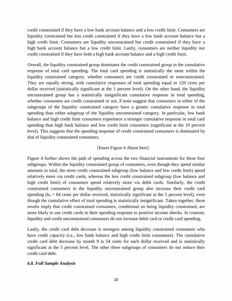
We also plot, in Figure 1b, the unconditional mean total spending of the treatment and control
group in the matched sample during the period of 2010:04 to 2011:11. On average, the treatment
group has a higher total spending than the control group. Moreover, the difference in total
spending between the treatment group and the control group before the announcement of the
Growth Dividend program remains constant, which confirms the underlying identifying
assumption of a parallel trend. Note that the gap between the treatment group and the control
group visibly increases after the program, which provides the first suggestive evidence of
consumer spending response to the income shock.
5. Methodology
We analyze the response of credit card spending, debit card spending, and checking account
balances as a function of the fiscal policy stimulus, beginning with the monthly individual-level
data. First, we study the average monthly spending response to the stimulus using the following
specifications:
The dependent variable represents the dollar amount of total card spending, debit card
spending, credit card spending, and credit card debt held by individual i at the end of month t.
Because the Growth Dividend is a temporary event and debt is a stock variable, to allow for
potentially persistent effects of the stimulus on debt, the specification for debt uses the change in
debt as the dependent variable. Spending is a flow variable and is therefore analyzed in levels.
is the amount of the Growth Dividend that individual i received, and is equal to zero
for the control group. is a binary variable equal to one for the months after the
announcement of the Growth Dividend Program (i.e., later than 2011:01). is the year-month
dummy, used to absorb the seasonal variation in consumption expenditures as well as the
average of all other concurrent aggregate factors, and is the individual dummy included to
absorb differences in consumption preferences at the individual level. The in Equation (1)
captures the average monthly spending (or debt) response per dollar received for a treated
individual after the announcement of the stimulus program, relative to the change in spending (or
debt) of the control group. We also divide the post-policy window into the announcement period
and the disbursement period, to compare the policy effect in these two windows separately.
is a binary variable equal to one for the months during the announcement window
(2011:02–2011:03), and is a binary variable equal to one for the months after the
disbursement of the Growth Dividends (i.e., later than 2011:04). Therefore, the coefficients
and in Equation (2) capture the average monthly spending (or debt) response per dollar
received, relative to the change in spending (or debt) of the control group, for a treated individual
during the announcement period and after the disbursement, respectively.
11
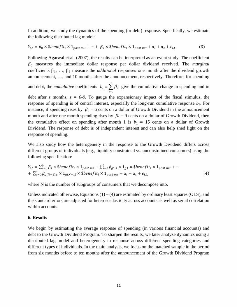
In addition, we study the dynamics of the spending (or debt) response. Specifically, we estimate
the following distributed lag model:
Following Agarwal et al. (2007), the results can be interpreted as an event study. The coefficient
measures the immediate dollar response per dollar dividend received. The marginal
coefficients 1, …, 9 measure the additional responses one month after the dividend growth
announcement, …, and 10 months after the announcement, respectively. Therefore, for spending
and debt, the cumulative coefficients
s
t
tsb0
give the cumulative change in spending and in
debt after s months, s = 0-9. To gauge the expansionary impact of the fiscal stimulus, the
response of spending is of central interest, especially the long-run cumulative response b9. For
instance, if spending rises by = 6 cents on a dollar of Growth Dividend in the announcement
month and after one month spending rises by = 9 cents on a dollar of Growth Dividend, then
the cumulative effect on spending after month 1 is 15 cents on a dollar of Growth
Dividend. The response of debt is of independent interest and can also help shed light on the
response of spending.
We also study how the heterogeneity in the response to the Growth Dividend differs across
different groups of individuals (e.g., liquidity constrained vs. unconstrained consumers) using the
following specification:
∑ ∑
∑
where N is the number of subgroups of consumers that we decompose into.
Unless indicated otherwise, Equations (1) – (4) are estimated by ordinary least squares (OLS), and
the standard errors are adjusted for heteroscedasticity across accounts as well as serial correlation
within accounts.
6. Results
We begin by estimating the average response of spending (in various financial accounts) and
debt to the Growth Dividend Program. To sharpen the results, we later analyze dynamics using a
distributed lag model and heterogeneity in response across different spending categories and
different types of individuals. In the main analysis, we focus on the matched sample in the period
from six months before to ten months after the announcement of the Growth Dividend Program

12
(2010:08–2011:11).8 To further address the possibility that individuals spend via financial
instruments issued by other banks, we include in our main analysis only individuals who had a
bank account, debit card, and credit card account with the bank at the same time.9
6.1. The average response of debit card and credit card spending and credit card debt
Panel A of Table 2 shows the average response from applying Equation (1) to spending and the
change in credit card debt. The first column shows the average response of monthly total card
spending (i.e., debit card spending + credit card spending) of the treatment group. Overall,
individuals in the treatment group increase their card spending by 8.9 cents per month for every
dollar of Growth Dividend received. The effect is both statistically and economically significant,
and it corresponds to a total increase of 89 cents per dollar received. More than two thirds of the
total spending increase after the stimulus program announcement is attributable to the spending
increase on credit cards (67 cents per dollar received, column 3 of Table 2, Panel A), and less
than one third is due to spending on debit cards (22 cents per dollar received, column 2 of Table
2, Panel A). Credit card debt experiences a 1.1 cents decrease per month or an 11-cent decrease
in total per dollar received for the treatment group after the announcement, but the effect is only
statistically significant at the 10 percent level.
[Insert Table 2 About Here]
6.2. Announcement vs. disbursement effect
The Growth Dividend Program was a one-time stimulus program that was unprecedented and
unanticipated by the population in Singapore. In addition, the program was announced with full
information on the eligibility, timing, and size of the pay out in February 2011, two months
before qualified Singaporeans received the payments in April 2011. As a result, we can
investigate the announcement effect separately from the disbursement effect. The prior literature
has not been unsuccessful at estimating the announcement effect because the announcement was
anticipated. This weakened the identification of the announcement effect. However, the
life-cycle theory has a clear prediction that consumers should respond to the announcement. Our
setting is the first to cleanly test this theory: the two prior papers (Poterba 1988 and Wilcok 1989)
that look at this effect had weaker identification between announcement and disbursement. We
thus estimate Equation (2) by decomposing the post-policy window into the announcement
period and the disbursement period (Table 2, Panel B).
We find a significant increase in total card spending in both windows: individuals spent 8 cents
per month for every dollar received in the two-month announcement period and 9.2 cents per
8 We are restricted by data availability to looking at 10 months after the Growth Dividend Program, but this period is
sufficient for our purposes, as the consumption response converges over this time period. Agarwal et al. (2007) also
use a similar lag structure. 9 We include individuals with fewer than three accounts with the bank in the analysis as a robustness check, and our
results remain qualitatively the same.

13
month for every dollar received during the disbursement period. Interestingly, there is a
significant difference in the means of spending for the two windows. For the announcement
period, the increase in spending is primarily concentrated in credit cards (7.1 cents per month for
one dollar received), while there is no statistically or economically significant change in debit
card spending for the treatment group during this period. Debit card spending increases mostly in
the disbursement window, and the credit card spending continues to be higher than the pre-policy
period for the treatment group during the disbursement window. Similarly, there is little change
in credit card debt during the announcement period, and consumers start to pay down their credit
card debt after they receive the Growth Dividend (consistent with Agarwal et al. 2007).
In summary, consumers started spending the stimulus money upon announcement of the program,
before the actual receipt of the dividend. Compared to the disbursement window, they increased
spending in the announcement period by a similar amount, primarily through credit card use.
After receiving the dividend, they used their debit cards along with credit cards to increase
spending. Consumers also started to pay down debt after receiving the money.
6.3. Response in bank checking accounts
We next study debit transactions in consumers’ bank checking accounts before and after the
announcement of the Growth Dividend Program. Because we do not have transaction-level data
on debit transactions in the checking accounts, we use the number of debit transactions as the
dependent variable to investigate whether consumers in the treatment group increased the
number of debit transactions significantly after the program. Table 3 shows the regression results.
There is no significant change in the number of checking account debit transactions after the
stimulus program for the treatment group. We also decompose debit transactions into ATM,
in-branch, and online transactions and find no significant change in the activity in any of the
three categories for the treatment group after the program. This result suggests that most likely
consumers increased their spending through card spending, either with debit or credit cards.10
[Insert Table 3 About Here]
6.4. Heterogeneity in spending response: by spending category
The extant literature documents heterogeneity in the type of spending response to positive
income shocks (e.g., Parker et al. 2013). We select several major spending categories into which
we decompose the total monthly card spending for each individual. Table 4 shows the estimation
results of the average spending response by spending category. As in Tables 2 and 3, we use the
10
We perform an additional test by inferring the amount of monthly cash/check spending for each individual. By
assuming that individuals deposit their monthly income into and pay their credit card balance from this particular
bank’s account, we estimate (a noisy measure of) the monthly cash/check spending as bank balance at the start of the
month+ income – total card spending – bank balance at the end of the month. In an unreported regression, we find that
there is no difference in the change of cash/check spending between the treatment group and the control group, which
is consistent with the finding on the number of bank transactions in Table 3.

14
dollar amount of spending as the dependent variable in Panel A of Table 4, so the coefficient
captures the spending response in dollars for every dividend dollar received. Discretionary
spending categories, such as apparel and travel, respond the most to the stimulus program. For
each dollar of Growth Dividend received, consumers spend 1.6–1.7 cents per month, or 16–17
cents in total in our sample period, on apparel or travel purchases. Consumers also seem to
increase their spending in other categories such as supermarket, dining, entertainment, and
transportation, but the economic and statistical effect is weaker than the increases in apparel and
travel spending.
[Insert Table 4 About Here]
In Panel B of Table 4, we use the log of spending as the dependent variable, and the key
explanatory variable is the interaction term of the treatment dummy and post-announcement
dummy. The coefficient in this specification captures the percentage change in spending after the
stimulus program relative to the pre-stimulus spending level in that category. Overall, consumer
spending increases in the treatment group by 13.5% in apparel, 8.8% in travel, 7.6% in
transportation, and 11.1% in entertainment. These results are statistically significant (at the 1
percent or 5 percent level) and economically large. In particular, although consumers do not
appear to spend a significant amount (in absolute terms) on entertainment, the spending increase
is large as a proportion of their pre-stimulus spending in entertainment. In sum, spending
responds to the stimulus program across spending categories, but the effect is strongest in the
discretionary spending categories (entertainment, apparel, and travel).
6.5. The dynamics of the spending and debt response
Results in Tables 2–4 show the average monthly response of spending and debt to the stimulus
program. In addition, to gauge the expansionary impact of the fiscal stimulus, we investigate the
dynamic evolution of the spending and debt response during the 10-month period beginning with
the program announcement (Equation (3)). Table 5 reports the marginal coefficients, βs, s = 0-9.
Figure 2 graph the entire paths of cumulative coefficients bs, s = 0-9, along with their
corresponding 95 percent confidence intervals. The results can be interpreted as an event study,
with month 0 being the time of pay out receipt, s = 0 in event time.
[Insert Table 5 About Here]
[Insert Figure 2 About Here]
Starting with the point estimates for spending, in the stimulus announcement month, (monthly)
total card spending rises by 0 = b0 = 6.2 cents for every dollar of Growth Dividend received.
One month later, spending rises, compared to the pre-announcement period, by 1 = 9.9 cents on
a dollar of dividend received, so the cumulative increase b1 = 16.1 cents per dollar received in
the announcement period. For the first month of the disbursement period, total card spending
increases by another 15.2 cents per dollar, making the cumulative increase rise to b2 = 31.3 cents
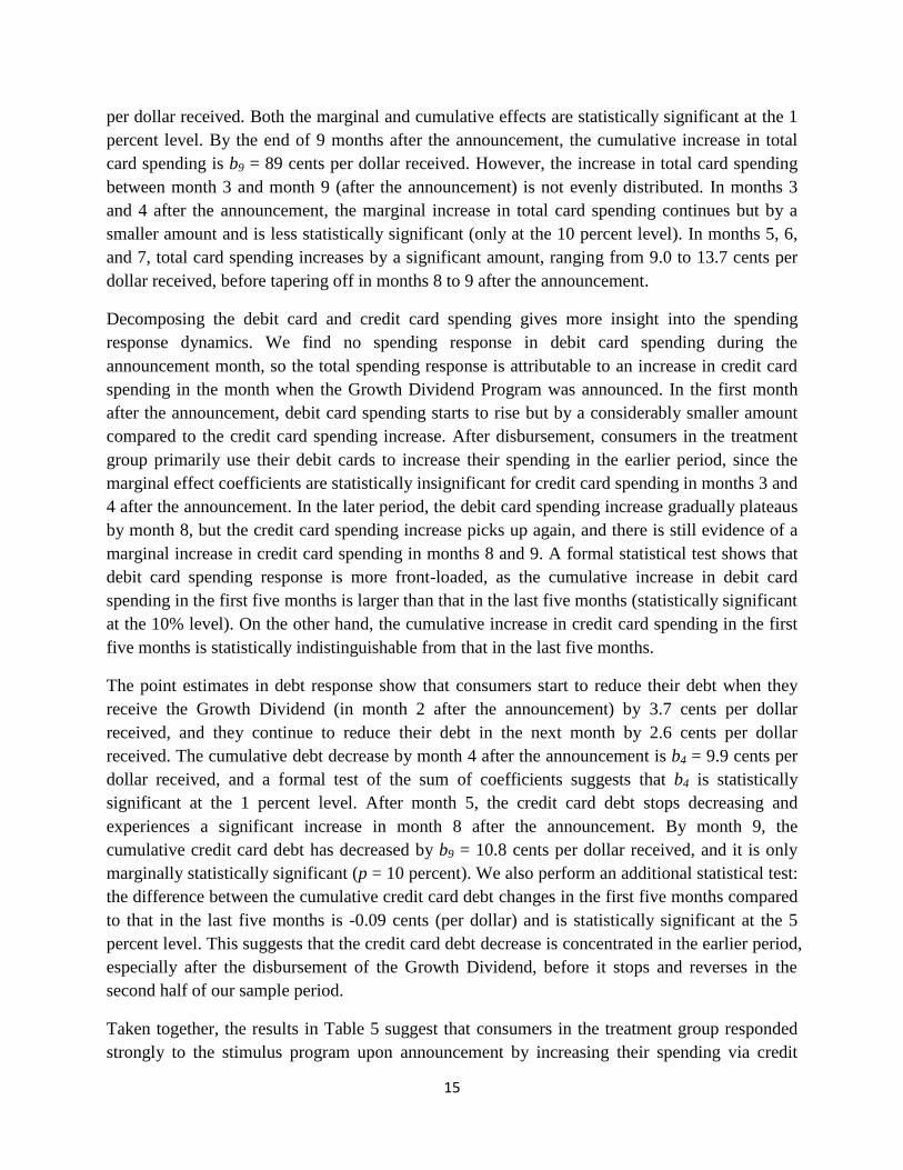
15
per dollar received. Both the marginal and cumulative effects are statistically significant at the 1
percent level. By the end of 9 months after the announcement, the cumulative increase in total
card spending is b9 = 89 cents per dollar received. However, the increase in total card spending
between month 3 and month 9 (after the announcement) is not evenly distributed. In months 3
and 4 after the announcement, the marginal increase in total card spending continues but by a
smaller amount and is less statistically significant (only at the 10 percent level). In months 5, 6,
and 7, total card spending increases by a significant amount, ranging from 9.0 to 13.7 cents per
dollar received, before tapering off in months 8 to 9 after the announcement.
Decomposing the debit card and credit card spending gives more insight into the spending
response dynamics. We find no spending response in debit card spending during the
announcement month, so the total spending response is attributable to an increase in credit card
spending in the month when the Growth Dividend Program was announced. In the first month
after the announcement, debit card spending starts to rise but by a considerably smaller amount
compared to the credit card spending increase. After disbursement, consumers in the treatment
group primarily use their debit cards to increase their spending in the earlier period, since the
marginal effect coefficients are statistically insignificant for credit card spending in months 3 and
4 after the announcement. In the later period, the debit card spending increase gradually plateaus
by month 8, but the credit card spending increase picks up again, and there is still evidence of a
marginal increase in credit card spending in months 8 and 9. A formal statistical test shows that
debit card spending response is more front-loaded, as the cumulative increase in debit card
spending in the first five months is larger than that in the last five months (statistically significant
at the 10% level). On the other hand, the cumulative increase in credit card spending in the first
five months is statistically indistinguishable from that in the last five months.
The point estimates in debt response show that consumers start to reduce their debt when they
receive the Growth Dividend (in month 2 after the announcement) by 3.7 cents per dollar
received, and they continue to reduce their debt in the next month by 2.6 cents per dollar
received. The cumulative debt decrease by month 4 after the announcement is b4 = 9.9 cents per
dollar received, and a formal test of the sum of coefficients suggests that b4 is statistically
significant at the 1 percent level. After month 5, the credit card debt stops decreasing and
experiences a significant increase in month 8 after the announcement. By month 9, the
cumulative credit card debt has decreased by b9 = 10.8 cents per dollar received, and it is only
marginally statistically significant (p = 10 percent). We also perform an additional statistical test:
the difference between the cumulative credit card debt changes in the first five months compared
to that in the last five months is -0.09 cents (per dollar) and is statistically significant at the 5
percent level. This suggests that the credit card debt decrease is concentrated in the earlier period,
especially after the disbursement of the Growth Dividend, before it stops and reverses in the
second half of our sample period.
Taken together, the results in Table 5 suggest that consumers in the treatment group responded
strongly to the stimulus program upon announcement by increasing their spending via credit

16
cards. We find a delayed spending response via debit cards, which occurred only after the
payment of the stimulus money and then gradually plateaued over time. At the same time,
consumers started to decrease their credit card debt as well as reduce their credit card spending in
the early period after the disbursement. However, in the last few months of the ten-month
treatment period, they stopped paying down their credit card debt and increased their credit card
spending significantly again.
6.6. Heterogeneity of spending and debt response across consumers
We next study the dynamics of heterogeneous responses to the financial stimulus program across
different consumers. Previous literature has shown that the consumption of liquidity constrained
consumers responds more strongly to positive income shocks (e.g., Agarwal et al. 2007). We
have a rich array of account-holder information, including their demographics and financial
health information, which allows us to study the heterogeneous response of consumers in greater
depth.11
Furthermore, our data allow us to understand differences in the full path of the
consumers’ spending and debt responses across different financial instruments. In the following
subsections, we estimate Equation (4) by interacting for each group of comparison of consumers.
To save space, we do not report the marginal effect coefficients. Instead, we plot the cumulative
response coefficients, bs, s = 0-9, along with their corresponding 95 percent confidence intervals
(Figure 3).
[Insert Figure 3 About Here]
A. Low Checking Account Balance vs. High Checking Account Balance
We classify consumers in our sample as having a low checking account balance if their average
monthly checking account balance in the four months before our analysis sample (i.e., 2010:04–
2010:07) is below the 25th
percentile of the distribution, or equivalently SGD 1,840 in the
cross-section of consumers in that period. Consumers have a high checking account balance if
their average monthly balance in that period is above the 75th
percentile of the distribution, or
SGD 22,346. Consumers with low checking account balances are likely to be more liquidity
constrained.
Panel A of Figure 3 shows the comparison in the path of spending and debt response between
these two groups of consumers. Low-balance consumers respond strongly via debit card
spending: for each dollar of stimulus payment, b9 = 50 cents for low-balance consumers, and the
effect is statistically significant at the 1 percent level. In particular, low-balance consumers start
spending on debit cards from the second month of the announcement period and continue to
experience a significant increase until month 7, after which the debit card spending increase
11
Earlier studies use demographics as proxies for liquidity constrained consumers. For instance, the papers argue that
young and old consumers are more likely to be liquidity constrained. Additionally, married consumers are less likely
to be liquidity constrained.

17
plateaus. There is also a strong cumulative increase in credit card spending among low-balance
consumers: b9 = 76 cents for each dollar received, which is statistically significant at the 1
percent level. On the other hand, high-balance consumers do not increase debit card spending,
and their cumulative credit card spending increase by month 9 is equal to 47 cents per dollar
received, which is smaller than that of the low-balance consumers. We perform a formal test of
the difference in total cumulative spending response between low-balance and high-balance
consumers. We run an OLS regression of total spending and run an F-test of the difference in the
cumulative coefficients b9 between the two groups. The result is statistically significant at the 1
percent level, indicating that low-balance consumers spend more via debit cards and credit cards
than high-balance consumers.
Low-balance consumers start to pay down their credit card debt upon receipt of the stimulus
money (month 2 after the announcement), and by month 9, the cumulative debt decrease is 18
cents per dollar received and is statistically significant at the 5 percent level. In contrast, there is
no change in credit card debt among high-balance consumers. These results are consistent with
the literature: liquidity constrained consumers react strongly to the stimulus in spending, and
they also use the positive income shock to reduce their credit card debt.
B. High Credit Card Limit vs. Low Credit Card Limit
We classify consumers in our sample as having a high credit card limit if their maximum credit
card limit in the four months before our analysis sample (i.e., 2010:04–2010:07) is above the
75th percentile of the distribution, or equivalently SGD 9,000 in the cross-section of consumers
during that period. Consumers have a low credit card limit if their maximum credit card limit
between 2010:04 and 2010:07 is below the 25th percentile of the sample, or SGD 5,000. This is
another measure to capture liquidity constrained consumers that has been used in previous
studies.
Panel B of Figure 3 shows the comparison across these two groups of consumers. High credit
card limit consumers show little spending response, regardless of the financial instruments. The
cumulative spending coefficients for both credit cards and debit cards are statistically
insignificant throughout the period. Low credit limit consumers react to the stimulus program by
increasing both their debit card and credit card spending. However, the effect is stronger on
credit card spending. The cumulative debit card spending increase at month 9 after the program
announcement is b9 = 19 cents per dollar received and is statistically significant at the 5 percent
level. Credit card spending has a cumulative increase of 87 cents per dollar received by month 9,
and the effect is statistically significant at the 1 percent level. An F-test of the cumulative
coefficients of total spending suggests that low credit limit consumers’ total spending response is
greater than that of high credit limit consumers (difference = 79 cents and is statistically
significant at the 1 percent level).

18
While low credit limit consumers see no credit card debt change during the 10-month period,
high credit limit consumers’ credit card debt decreases strongly: by month 9, the cumulative
credit card debt change is -27 cents per dollar received, and this effect is statistically significant
at the 1 percent level.
C. Low Income vs. High Income
We classify consumers in our sample as low-income consumers if their average monthly income
in the year before the stimulus program (2010) was below the 25th
percentile of the distribution,
or equivalent to SGD 3,049, in the cross-section of consumers in that period. High-income
consumers are those with an average monthly income in 2010 above the 75th
percentile of the
distribution (or SGD 6,369). Panel C shows that low-income consumers react strongly to the
stimulus program in spending. For low-income consumers, the cumulative coefficient by month
9 is 20 cents per dollar received (statistically significant at the 5 percent level) for debit card
spending, and is 61 cents per dollar received (statistically significant at the 1 percent level) for
credit card spending. For high-income consumers, the cumulative coefficients for both debit card
spending and credit card spending are statistically insignificant. However, the F-test shows that
the cumulative total spending response is not statistically different between the low-income
consumers and the high-income consumers. The weaker result for the low-income consumers,
although still broadly consistent with the findings of low bank balance and low credit card limit
consumers, may be due to income being a noisier measure of liquidity constraint.
D. Young vs. Old
We compare the spending and debt response pattern for younger (2010 age ≤ 25th
percentile = 32)
and older consumers (2010 age ≥ 75th
percentile = 42) in Panel D. Younger consumers have
positive and significant cumulative spending responses: b9 = 36 cents for every dollar received
for debit card spending, and b9 = 73 cents for credit card spending. Older consumers do not
increase their debit card spending, but their cumulative credit card spending increase is
significant: b9 = 71 cents per dollar received, which is significant at the 1 percent level. The
overall spending response of the young is larger—39 cents per dollar received—and is
statistically significant at the 10 percent level according to the F-test. In addition, we observe a
credit card debt decrease among the older consumers. They start paying down their credit card
debt from month 1 after the program announcement, and by the end of month 9, their cumulative
credit card debt decrease is 16 cents for every dollar received (statistically significant at the 5
percent level).
E. Married vs. Non-married
We compare the spending and debt response pattern for married and non-married consumers in
Panel E. Overall, the total spending response is comparable between the two groups: the
cumulative coefficients of total card spending are statistically indistinguishable between married

19
and non-married consumers. Married consumers pay down their credit card debt upon receiving
the stimulus money (month 2), and the cumulative credit card debt change is b9 = -15 cents for
every dollar received (statistically significant at the 5 percent level). Non-married consumers, on
the other hand, do not reduce their credit card debt during the 10-month period.
F. Ethnicity: Chinese vs. Indian
Chinese, Malay, and Indian are three major ethnic groups in Singapore, and we compare the
difference in spending and debt response between Chinese Singaporeans and Indian
Singaporeans in Panel F. (Malays are dropped from the analysis due to their small sample size in
our data.) Chinese Singaporeans significantly increase their spending on both types of cards,
though more so on credit cards (b9 = 67 cents for credit cards vs. b9 = 22 cents for debit cards).
Indian Singaporeans, in comparison, have an insignificant cumulative spending response for both
instruments. However, the F-test result shows that the difference in the cumulative response of
total spending between the two groups is not statistically different from zero. In addition, Indians
save more on average. Compared to Chinese Singaporeans, whose credit card debt remains flat
during the 10-month period, Indian Singaporeans reduce their credit card debt significantly (b9 =
-43 cents for every dollar received, significant at the 1 percent level).
G. Male vs. Female
Lastly, we compare the gender difference in spending and debt response to the stimulus program
(Panel G). The cumulative increase in debit card spending by month 9 after the program
announcement is strong for male consumers (b9 = 26 cents for every dollar received, significant
at the 1 percent level) but insignificant for female consumers (b9 = 12 cents). Both groups
respond strongly in credit card spending: b9 = 74 cents for male consumers, and b9 = 50 cents for
female consumers, both significant at the 1 percent level). Overall, an F-test of the cumulative
coefficients of total spending suggests that male consumers have a stronger response in total
spending (by 38 cents per dollar received, statistically significant at the 5 percent level). Male
consumers start to pay down debt upon receiving the money (month 2). Their cumulative credit
card debt decrease is 11 cents per dollar received by month 9 and is statistically significant at the
10 percent level.
6.7. Liquidity vs. credit constraint
Due to data limitations, previous studies often use credit card capacity (i.e., credit constraints) to
proxy for liquidity constraints.12
In this section, we examine the differences in the spending and
debt responses of liquidity constrained consumers (i.e., those with low checking account
balances) and credit constrained consumers. We further classify consumers as both liquidity and
12
The existing literature focuses on the credit card capacity as the main measure of credit constraints since it is
arguably more exogenous than credit card balance and credit card utilization (balance divided by credit card limit) ,
which are measures based on (endogenous) spending choice of individuals (see Agarwal, Liu, and Souleles, 2007).
20
credit constrained if they have a low bank account balance and a low credit limit. Consumers are
liquidity constrained but less credit constrained if they have a low bank account balance but a
high credit limit. Consumers are liquidity unconstrained but credit constrained if they have a
high bank account balance but a low credit limit. Lastly, consumers are neither liquidity nor
credit constrained if they have both a high bank account balance and a high credit limit.
Overall, the liquidity constrained group dominates the credit constrained group in the cumulative
response of total card spending. The total card spending is statistically the same within the
liquidity constrained category, whether consumers are credit constrained or nonconstrained.
They are equally strong, with cumulative responses of total spending equal to 120 cents per
dollar received (statistically significant at the 1 percent level). On the other hand, the liquidity
unconstrained group has a statistically insignificant cumulative response in total spending,
whether consumers are credit constrained or not. F-tests suggest that consumers in either of the
subgroups of the liquidity constrained category have a greater cumulative response in total
spending than either subgroup of the liquidity unconstrained category. In particular, low bank
balance and high credit limit consumers experience a stronger cumulative response in total card
spending than high bank balance and low credit limit consumers (significant at the 10 percent
level). This suggests that the spending response of credit constrained consumers is dominated by
that of liquidity constrained consumers.
[Insert Figure 4 About here]
Figure 4 further shows the path of spending across the two financial instruments for these four
subgroups. Within the liquidity constrained group of consumers, even though they spend similar
amounts in total, the more credit constrained subgroup (low balance and low credit limit) spend
relatively more via credit cards, whereas the less credit constrained subgroup (low balance and
high credit limit) of consumers spend relatively more via debit cards. Similarly, the credit
constrained consumers in the liquidity unconstrained group also increase their credit card
spending (b9 = 64 cents per dollar received, statistically significant at the 5 percent level), even
though the cumulative effect of total spending is statistically insignificant. Taken together, these
results imply that credit constrained consumers, conditional on being liquidity constrained, are
more likely to use credit cards in their spending response to positive income shocks. In contrast,
liquidity and credit unconstrained consumers do not increase debit card or credit card spending.
Lastly, the credit card debt decrease is strongest among liquidity constrained consumers who
have credit capacity (i.e., low bank balance and high credit limit consumers). The cumulative
credit card debt decrease by month 9 is 54 cents for each dollar received and is statistically
significant at the 5 percent level. The other three subgroups of consumers do not reduce their
credit card debt.
6.8. Full Sample Analysis

21
We perform the main analysis in the previous sections on a smaller sample in which the
treatment group and control group are matched on several demographic variables. To ensure that
the results can be generalized to the full sample, we repeat the estimation in Equations (1) and (2)
on the unmatched sample and report the results in Table 6.
[Insert Table 6 About Here]
The first column of Table 6, Panel A shows that consumers in the treatment group increase their
card spending by a total of 46 cents for every dollar received during the 10-month period. Like
before, over two thirds of the total spending increase is attributable to the spending increase via
credit cards (30 cents per dollar received, column 3 of Table 6, Panel A), and less than one third
is due to spending on debit cards (16 cents per dollar received, column 2 of Table 6, Panel A).
Credit card debt experiences a statistically insignificant 3-cent decrease in total per dollar
received during the 10-month period for the treatment group. Similarly, consumers in the
treatment group increase their spending more on their credit cards during the announcement
period and then switch to debit card use after disbursement. Overall, the results on the full
unmatched sample remain qualitatively the same. The somewhat smaller magnitude of the effect
is expected, as the (unmatched) control group has higher income and wealth than the (unmatched)
treatment group (Table 1, Panel A) and likely has a higher spending level and growth. Therefore,
the estimated coefficients from the full sample are downward biased and should be viewed as a
lower bound of the stimulus response.
6.9. Robustness checks
In this section, we perform and discuss a series of tests to study the robustness of our results. For
brevity, we do not report the tables which are available upon request.
About 40% of the population of Singappore are foreigners. While a majority of them are from
China, India, Malaysia, and Indonesia, there are quite a large proportion from Australia, Europe
and Ameirca. It is possible that foreigners (as our control group) in general may differ from
Singaporeans (our treatment group) in their consumption preferences and habits, which will
confound our interpretation of the difference-in-difference analysis. We address the potential
concern by restricting the control group to consumers with the following nationalities: Malaysia,
China, India, and Indonesia. These foreigners either come from neighboring countries or have
similar ethnic and cultural backgrounds as Singaporeans. As a result, they have a tighter bond
with the country and likely share the same consumption preferences or/and habits as consumers
in our treatment group. Using the smaller control group with these restricted foreigners, we
repeat the difference-in-difference analysis and our results are both qualitatively and
quantitatively very similar.
It is still possible that foreigners are different in unobservable ways, so we perform an additional
robustness analysis by completely dropping the foreigners from the sample. Instead, we exploit
the heterogeneity in the payout amount within the treated group and use the Singaporeans with

22
the smallest amount of the Growth Dividend, i.e., those with an annual income greater than SGD
100,000, as the control group. We continue to find a very significant increase in the total
spending after the dividend program.
In the main analysis, we dropped from our sample Singaporeans who also qualified for another
cash stimulus program announced at the same time. To further isolate the response to the Growth
Dividend Program from other concurrent stimulus packages, we first note that there is a
concurrent personal income tax rebate worth a total of US$452.4 million, which is one third of
the size of the Growth Dividend Program. Because the tax rebate applies to all working residents
in Singapore based entirely on income level, a foreigner is entitled to the same amount of tax
rebate as another Singaporean with the same annual income in 2010. Because the control group
and the treatment group in the matched sample have comparable income levels (the difference is
economically and statistically insignificant, as in Table 1 Panel B and Figure 1), the spending
and debt response to the tax rebate are differenced out in our estimation, and our coefficients are
the incremental response beyond the tax rebate program. Lastly, the only other economically
significant package (US$393.1 million) targeted older Singaporeans (age ≥ 45) by topping up
their illiquid retirement medical accounts, which can only be applied to hospitalization or certain
out-patient care items and cannot be cashed out. We verify our results in a separate analysis on a
subsample of consumers younger than 45 years old who are entitled only to the Growth Dividend
Program.
We further study whether the documented consumption response is due to the Growth Dividend
program or attributable to general government subsidies that usually occur in the month of April.
We compare the total spending difference between the treatment group and the control group in
April of 2011 (our event year) with the difference in April of 2010.13
We find that consumers in
the treatment group spend significantly more than those in the control group in April of 2011, but
their total spending is smaller than that of the same control group in April 2010 and the
difference is statistically indistinguishable from zero. This result suggests that our findings on the
consumption (and debt) response are unlikely to be explained by other government subsidies or
an April effect.
We also perform falsification tests by carrying out the difference-in-differences analysis on the
treatment and control groups using randomly picked dates for the stimulus program. Specifically,
we choose June, 2011 (i.e., 4 months after the stimulus program) and October, 2010 (i.e., 4
months before the stimulus program), and study whether the treatment group’s spending and debt
change, relative to the control group, in the two month period after the chosen month compared
to the previous two months. Our results show that there are no spending (and debt) responses
after both (random) dates, which suggests that our estimates in the main analysis capture the
response to the specific stimulus program announced in February, 2011.
13
Ideally we want to perform a similar difference-in-difference analysis around April in other years. However, we
only have two years of data which begins in April 2010 and hence our data does not allow such analysis.

23
Lastly, to address the possibility that the stimulus program coinsides with the timing of the
annual bonus disbtribution and that Singaporeans (treatment) and foreigners (control) may
receive different bonus amounts, we restrict our sample to non-salaried consumers who do not
receive bonuses and our results remain robust.14
7. Conclusion
This paper uses a unique, new panel data set of credit card, debit card, and checking account
information for more than 180,000 consumers in Singapore to analyze how consumers responded
to a fiscal stimulus program announced on February 18th, 2011. The government distributed a
one-time payout of Growth Dividends to all Singaporeans over 21 years old in 2011. The
program’s payments totaled US$1.17 billion, which corresponds to 12 percent of Singapore’s
monthly aggregate household consumption expenditure in 2011. We used a diff-in-diff
identification to estimate the month-by-month response to the program of credit card spending,
debit card spending, and debt. Foreigners were not eligible for the Growth Dividend; this
exclusion restriction allows us to cleanly identify the causal effect of the program on spending by
using foreigners as our control group.
We find that consumption rose significantly after the fiscal policy announcement: for each dollar
received, consumers on average spent 90 cents (aggregated across different financial accounts)
during the ten months after the announcement. Consumers’ credit card debt moderately
decreased during this period (so savings effectively increased). We also identify a strong
announcement effect: consumers started to increase spending during the two-month
announcement period before the cash payout. We also find that consumption response is
distributed across debit card (25 percent of the total response) and credit card (75 percent of the
total response) spending. More importantly, consumers started spending via credit cards during
the announcement period, then switched to debit cards after disbursement, before finally
significantly increasing their credit card usage. Consistent with previous research, credit card
debt dropped in the first months after disbursement and then reverted back to pre-announcement
levels.
We also found other significant heterogeneity in the response to the fiscal stimulus across
different types of consumers. Notably, spending rose most among consumers who were,
according to various criteria, initially most likely to be liquidity constrained. Similarly, debt
declined most (so savings rose most) among liquidity constrained consumers. Comparing
liquidity constraints with credit constraints, we find that the spending response of the credit
constrained consumers is dominated by that of the liquidity constrained consumers. Liquidity
constrained consumers respond strongly to the stimulus, whether they are credit constrained or
not. Finally, consumption rose primarily in the non-food, discretionary category (consistent with
14
From the reported occupation, we identify consumers who are self-employed, housewives, retirees, non-workers, or
students as non-salaried.

24
Johnson et al. 2006). These results suggest that liquidity constraints are important. More
generally, the results suggest that there can be important dynamics in consumers’ responses to
“lumpy” increases via fiscal stimulus programs, working in part through balance sheet (liquidity)
mechanisms.
Our main contribution in relation to prior literature is three-fold. First, we are the first to document
the announcement effect of this stimulus program, which is of comparable magnitude of the
consumption response after disbursement. It also provides new evidence consistent with theory
predictions. Second, we document the dynamics of consumption response across different
spending instruments—a rise in credit card spending following the program’s announcement, then
the switch to debit card spending after the disbursement of the stimulus, and finally the switch
back to credit card spending in the later months. Finally, we are also the first to document that
liquidity constraints dominate credit constraints in regard to the spending response to positive
income shocks. Our paper can also help inform the design of fiscal policy. Our results suggest that
the announcement of a fiscal stimulus program can cause a consumption response, even before the
disbursement of the stimulus funds. Typically, policy makers announce fiscal programs over a
long time horizon, dampening the announcement effect of the stimulus program. Finally, in the
context of Singapore, our results provide support for the 2013 fiscal budget released by the
Ministry of Finance in Singapore, which allocates future stimulus to liquidity constrained
consumers.

25
References
Aaronson, Daniel, Sumit Agarwal, and Erik French. 2012. “Spending and Debt Response to
Minimum Wage Hikes.” American Economic Review 102 (7): 3111-39.
Agarwal, Sumit, Amit Bubna, and Molly Lipscomb. 2013. “Timing to the Statement:
Understanding Fluctuations in Consumer Credit Use.” University of Virginia Working Paper.
Agarwal Sumit, Souphala Chomsisengphet, Teck-Hua Ho and Wenlan Qian. 2013. “Cross
Border Shopping: Do Consumers Respond to Taxes or Prices?” Working Paper, National
University of Singapore
Agarwal, Sumit, Chunlin Liu, and Nicholas Souleles. 2007. "The Reaction of Consumption and
Debt to Tax Rebates: Evidence from the Consumer Credit Data." Journal of Political Economy
115 (6): 986-1019.
Agarwal, Sumit and Leslie McGranahan. 2013. “Consumption Response to State Sales Tax
Holidays.” Federal Reserve Bank of Chicago Working Paper.
Auerbach, A.J. 2002. “The Bush Tax Cut and National Saving.” National Tax Journal 55:
387-407.
Bertrand, Marianne, and Adair Morse. 2009. “What Do High-Interest Borrowers Do with their
Tax Rebate?" American Economic Review 99 (2): 418-423.
Blinder, A.S. 1981. “Temporary Income Taxes and Consumer Spending.” Journal of Political
Economy 89: 26-53.
Blinder, A.S., and A. Deaton. 1985. “The Time Series Consumption Function Revisited.”
Brookings Papers on Economic Activity 2: 465-511.
Bodkin, R. 1959. “Windfall Income and Consumption.” American Economic Review 49:
602-614.
Browning, M., and M.D. Collado. 2003. “The Response of Expenditures to Anticipated Income
Changes: Panel Data Estimates.” American Economic Review 91: 681-92.
Carroll, C. 1992. “The Buffer-Stock Theory of Saving: Some Macroeconomic Evidence.”
Brookings Papers on Economic Activity 2: 61-156.
Coulibaly, Brahima, and Geng Li. 2006. “Do Homeowners Increase Consumption after the Last
Mortgage Payment? An Alternative Test of the Permanent Income Hypothesis.” The Review of
Economics and Statistics 88: 10-19.
Fu, Y., W. Qian, and B. Yeung. 2012. “Transaction Tax and Speculators.” Working paper,
National University of Singapore.
Gross, D., and N. Souleles. 2002. “Do Liquidity Constraints and Interest Rates Matter for
Consumer Behavior? Evidence from Credit Card Data.” Quarterly Journal of Economics: 149-85.

26
Gross, Tal, Matthew Notowidigdo, and Jialan Wang. 2012. “Liquidity Constraints and Consumer
Bankruptcy: Evidence from Tax Rebates.” The Review of Economics and Statistics, forthcoming.
Hsieh, C. 2003. “Do Consumers React to Anticipated Income Changes? Evidence from the
Alaska Permanent Fund.” American Economic Review 93: 397-405.
Jappelli, T., S. Pischke, and N.S. Souleles. 1998. “Testing for Liquidity Constraints in Euler
Equations with Complementary Data Sources.” The Review of Economics and Statistics 80:
251-62.
Jappelli, Tullio and Luigi Pistaferri, 2010, “The Consumption Response to Income Changes,"
Annual Review of Economics, 2, 479-506.
Johnson, David, Jonathan Parker, and Nicholas Souleles. 2006. "Consumption and Tax Cuts:
Evidence from the Randomized Income Tax Rebates of 2001." American Economic Review 96:
1589-1610.
Leth-Petersen, Soren. 2010. “Intertemporal Consumption and Credit Constraints: Does
Consumption Respond to An Exogenous Shock to Credit?” American Economic Review
100:1080-1103.
Kreinin, M.E. 1961. “Windfall Income and Consumption: Additional Evidence.” American
Economic Review 51: 388-390.
Modigliani, F., and C. Steindel. 1977. “Is a Tax Rebate an Effective Tool for Stabilization
Policy?” Brookings Papers on Economic Activity 1: 175-209.
Parker, J. 1999. “The Reaction of Household Consumption to Predictable Changes in Social
Security Taxes.” American Economic Review 89: 959-73.
Parker, J., N. Souleles, D. Johnson, and R. McClelland. 2013. "Consumer Spending and the
Economic Stimulus Payments of 2008." forthcoming, American Economic Review.
Poterba, J.M. 1988. “Are Consumers Forward Looking? Evidence from Fiscal Experiments.”
American Economic Review 78: 413-18.
Shapiro, M.D., and J. Slemrod. 1995. “Consumer Response to the Timing of Income: Evidence
from a Change in Tax Withholding.” American Economic Review 85: 274-83.
Shapiro, M.D., and J. Slemrod. 2003a. “Consumer Response to Tax Rebates.” American
Economic Review 93: 381-96.
Shapiro, M.D., and J. Slemrod. 2003b. “Did the 2001 Tax Rebate Stimulate Spending? Evidence
from Taxpayer Surveys.” In Tax Policy and the Economy, edited by J. Poterba. Cambridge,
MA: MIT Press.
Shapiro, Jesse M. 2005. “Is There a Daily Discount Rate? Evidence from the Food Stamp
Nutrition Cycle.” Journal of Public Economics 89: 303-25.
Shea, J. 1995. “Union Contracts and the Life-Cycle/Permanent-Income Hypothesis.” American

27
Economic Review 85: 186-200.
Souleles, N.S. 1999. “The Response of Household Consumption to Income Tax Refunds.”
American Economic Review 89: 947-58.
Souleles, N.S. 2000. “College Tuition and Household Savings and Consumption.” Journal of
Public Economics 77 (2): 185-207.
Souleles, N.S. 2002. “Consumer Response to the Reagan Tax Cuts.” Journal of Public
Economics 85: 99-120.
Stephens, M. 2003. “3rd
of the Month: Do Social Security Recipients Smooth Consumption
Between Checks?” American Economic Review 93: 406-22.
Stephens, M. 2006. “Paycheck Receipt and the Timing of Consumption.” The Economic Journal
116 (513): 680-701.
Stephens, M. 2008. “The Consumption Response to Predictable Changes in Discretionary
Income: Evidence from the Repayment of Vehicle Loans.” The Review of Economics and
Statistics, 90(2): 241-52.
Wilcox, D.W. 1989. “Social Security Benefits, Consumption Expenditure, and the Life Cycle
Hypothesis.” Journal of Political Economy 97: 288-304.
Wilcox, D.W. 1990. “Income Tax Refunds and the Timing of Consumption Expenditure.”
Economic Activity Section Working Paper No. 106, Federal Reserve Board of Governors
working paper, April.

28
Figure 1: Summary Statistics of the Matched Sample
Figure 1a. shows the comparison of distributions of average monthly income in 2010, age, and average bank checking account balance during the period
2010:04–2010:07 between the treatment and control group, after the propensity score matching. Figure 1b. shows (logarithm of) the unconditional mean of total
spending of the treatment and control group during the period of 2010:04 to 2012:03.
1a. Kernel Density Plots of the Matched Sample
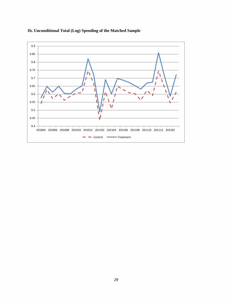
29
1b. Unconditional Total (Log) Spending of the Matched Sample
6.4
6.45
6.5
6.55
6.6
6.65
6.7
6.75
6.8
6.85
6.9
201004 201006 201008 201010 201012 201102 201104 201106 201108 201110 201112 201202
Control Treatment
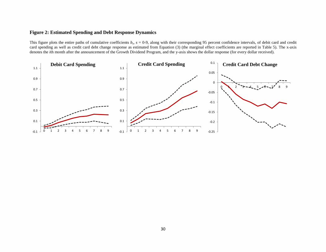
30
Figure 2: Estimated Spending and Debt Response Dynamics
This figure plots the entire paths of cumulative coefficients bs, s = 0-9, along with their corresponding 95 percent confidence intervals, of debit card and credit
card spending as well as credit card debt change response as estimated from Equation (3) (the marginal effect coefficients are reported in Table 5). The x-axis
denotes the ith month after the announcement of the Growth Dividend Program, and the y-axis shows the dollar response (for every dollar received).
-0.1
0.1
0.3
0.5
0.7
0.9
1.1
0 1 2 3 4 5 6 7 8 9
Debit Card Spending
-0.1
0.1
0.3
0.5
0.7
0.9
1.1
0 1 2 3 4 5 6 7 8 9
Credit Card Spending
-0.25
-0.2
-0.15
-0.1
-0.05
0
0.05
0.1
0 1 2 3 4 5 6 7 8 9
Credit Card Debt Change
31
Figure 3: Heterogeneity in Spending and Debt Response across Consumers
This figure plots the entire paths of cumulative coefficients bs, s = 0-9, along with their corresponding 95 percent confidence intervals, of spending and debt
response across different consumers. For each comparison panel, column (a) shows the cumulative debit card spending response, column (b) shows the
cumulative credit card spending response, and column (c) shows the cumulative credit card debt change response. The x-axis denotes the ith month after the
announcement of the Growth Dividend Program, and the y-axis shows the dollar response (for every dollar received). Panel A compares consumers with low
bank checking account balances (i.e., average checking account balance between 2010:04 and 2010:07 <= SGD 1,840, or 25% of sample) with consumers with
high bank checking account balances (i.e., average checking account balance between 2010:04 and 2010:07 >=SGD 22,346, or 75 percent of the sample). Panel
B compares consumers with high credit card limit (i.e., max credit card limit between 2010:04 and 2010:07 >= SGD 9,000, or 75 percent of the sample) with
consumers with low credit card limits (i.e., max credit card limit between 2010:04 and 2010:07 <= SGD 5,000). Panel C compares low-income consumers (i.e.,
monthly income in the year before the Growth Dividend announcement <= SGD 3,049, or 25 percent of the sample) with high-income consumers (i.e., monthly
income in the year before the Growth Dividend announcement >= SGD 6,360, or 75 of sample). Panel D compares younger consumers (age <= 32, or 25 percent
of the sample) and older consumers (age >= 42, or 75 percent of the sample). Panel E compares married and non-married consumers. Panel F compares different
ethnicities within the treated consumers (Chinese vs. Indian). Panel G compares male and female consumers.

32
Panel A:
(a) (b) (c)
Low Bank Balance
High Bank Balance
-0.4
-0.2
0
0.2
0.4
0.6
0.8
1
1.2
0 1 2 3 4 5 6 7 8 9
-0.4
-0.2
0
0.2
0.4
0.6
0.8
1
1.2
0 1 2 3 4 5 6 7 8 9
-0.4
-0.3
-0.2
-0.1
0
0.1
0.2
0.3
0 1 2 3 4 5 6 7 8 9
-0.4
-0.2
0
0.2
0.4
0.6
0.8
1
1.2
0 1 2 3 4 5 6 7 8 9
-0.4
-0.2
0
0.2
0.4
0.6
0.8
1
1.2
0 1 2 3 4 5 6 7 8 9
-0.4
-0.3
-0.2
-0.1
0
0.1
0.2
0.3
0 1 2 3 4 5 6 7 8 9

33
Panel B:
(a) (b) (c)
High Credit Card Limit
Low Credit Card Limit
-0.4
-0.2
0
0.2
0.4
0.6
0.8
1
1.2
0 0 0 0 0 0 0 0 0 0
-0.4
-0.2
0
0.2
0.4
0.6
0.8
1
1.2
0 0 0 0 0 0 0 0 0 0
-0.5
-0.4
-0.3
-0.2
-0.1
0
0.1
0 0 0 0 0 0 0 0 0 0
-0.4
-0.2
0
0.2
0.4
0.6
0.8
1
1.2
0 0 0 0 0 0 0 0 0 0
-0.4
-0.2
0
0.2
0.4
0.6
0.8
1
1.2
0 0 0 0 0 0 0 0 0 0
-0.5
-0.4
-0.3
-0.2
-0.1
0
0.1
0.2
0 0 0 0 0 0 0 0 0 0

34
Panel C:
(a) (b) (c)
Low Income
High Income
-0.4
-0.2
0
0.2
0.4
0.6
0.8
1
0 1 2 3 4 5 6 7 8 9
-0.4
-0.2
0
0.2
0.4
0.6
0.8
1
0 1 2 3 4 5 6 7 8 9
-0.3
-0.2
-0.1
0
0.1
0.2
0.3
0 1 2 3 4 5 6 7 8 9
-0.4
-0.2
0
0.2
0.4
0.6
0.8
1
0 1 2 3 4 5 6 7 8 9
-0.4
-0.2
0
0.2
0.4
0.6
0.8
1
0 1 2 3 4 5 6 7 8 9
-0.3
-0.2
-0.1
0
0.1
0.2
0.3
0 1 2 3 4 5 6 7 8 9

35
Panel D:
(a) (b) (c)
Young
Old
-0.3
-0.1
0.1
0.3
0.5
0.7
0.9
1.1
0 1 2 3 4 5 6 7 8 9
-0.3
-0.1
0.1
0.3
0.5
0.7
0.9
1.1
0 1 2 3 4 5 6 7 8 9
-0.35
-0.3
-0.25
-0.2
-0.15
-0.1
-0.05
0
0.05
0.1
0 1 2 3 4 5 6 7 8 9
-0.3
-0.1
0.1
0.3
0.5
0.7
0.9
1.1
0 1 2 3 4 5 6 7 8 9
-0.3
-0.1
0.1
0.3
0.5
0.7
0.9
1.1
0 1 2 3 4 5 6 7 8 9
-0.35
-0.3
-0.25
-0.2
-0.15
-0.1
-0.05
0
0.05
0.1
0 1 2 3 4 5 6 7 8 9
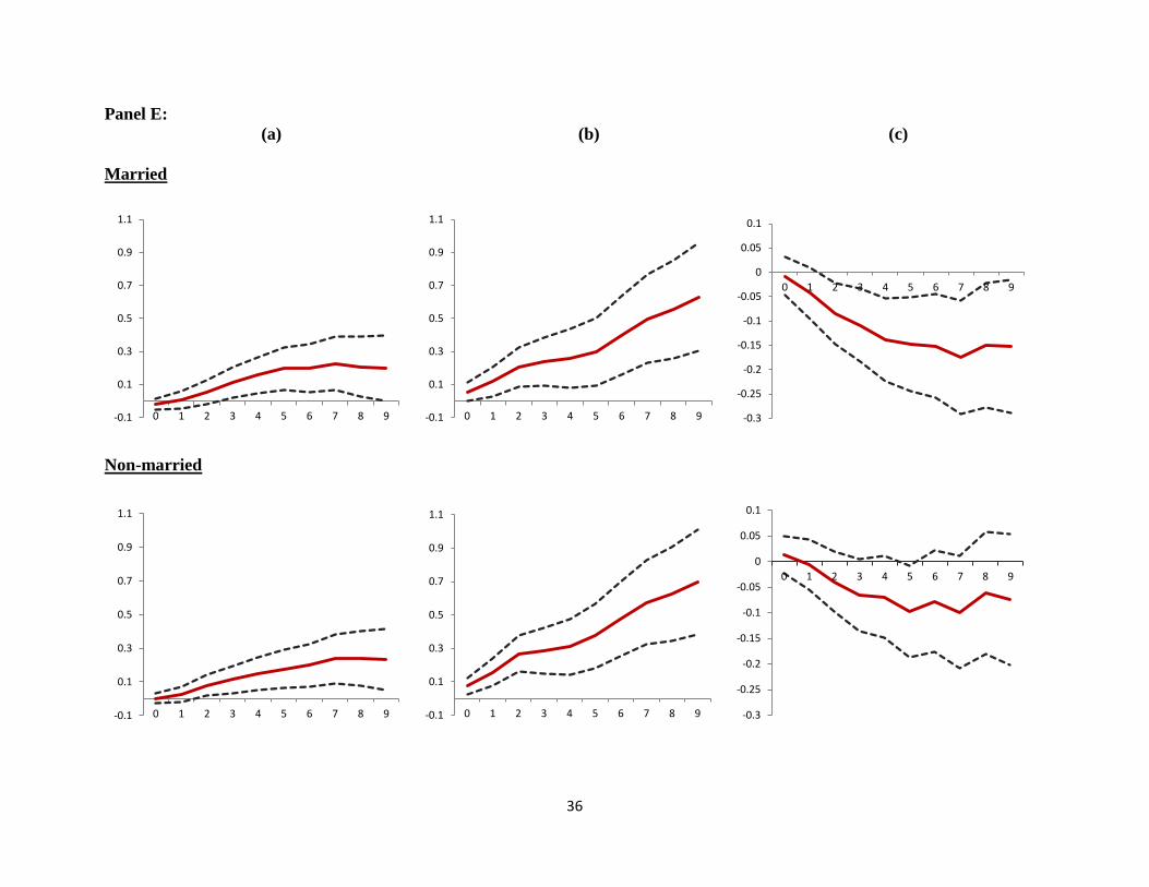
36
Panel E:
(a) (b) (c)
Married
Non-married
-0.1
0.1
0.3
0.5
0.7
0.9
1.1
0 1 2 3 4 5 6 7 8 9 -0.1
0.1
0.3
0.5
0.7
0.9
1.1
0 1 2 3 4 5 6 7 8 9 -0.3
-0.25
-0.2
-0.15
-0.1
-0.05
0
0.05
0.1
0 1 2 3 4 5 6 7 8 9
-0.1
0.1
0.3
0.5
0.7
0.9
1.1
0 1 2 3 4 5 6 7 8 9 -0.1
0.1
0.3
0.5
0.7
0.9
1.1
0 1 2 3 4 5 6 7 8 9 -0.3
-0.25
-0.2
-0.15
-0.1
-0.05
0
0.05
0.1
0 1 2 3 4 5 6 7 8 9

37
Panel F:
(a) (b) (c)
Chinese
Indian
-0.5
-0.3
-0.1
0.1
0.3
0.5
0.7
0.9
1.1
0 1 2 3 4 5 6 7 8 9
-0.5
-0.3
-0.1
0.1
0.3
0.5
0.7
0.9
1.1
0 1 2 3 4 5 6 7 8 9
-0.7
-0.6
-0.5
-0.4
-0.3
-0.2
-0.1
0
0.1
0 1 2 3 4 5 6 7 8 9
-0.5
-0.3
-0.1
0.1
0.3
0.5
0.7
0.9
1.1
0 1 2 3 4 5 6 7 8 9
-0.5
-0.3
-0.1
0.1
0.3
0.5
0.7
0.9
1.1
0 1 2 3 4 5 6 7 8 9
-0.7
-0.6
-0.5
-0.4
-0.3
-0.2
-0.1
0
0.1
0 1 2 3 4 5 6 7 8 9

38
Panel G:
(a) (b) (c)
Male
Female
-0.1
0.1
0.3
0.5
0.7
0.9
1.1
0 1 2 3 4 5 6 7 8 9 -0.1
0.1
0.3
0.5
0.7
0.9
1.1
0 1 2 3 4 5 6 7 8 9 -0.3
-0.25
-0.2
-0.15
-0.1
-0.05
0
0.05
0.1
0 1 2 3 4 5 6 7 8 9
-0.1
0.1
0.3
0.5
0.7
0.9
1.1
0 1 2 3 4 5 6 7 8 9 -0.1
0.1
0.3
0.5
0.7
0.9
1.1
0 1 2 3 4 5 6 7 8 9 -0.3
-0.25
-0.2
-0.15
-0.1
-0.05
0
0.05
0.1
0 1 2 3 4 5 6 7 8 9
39
Figure 4: Liquidity Constraints vs. Credit Constraints
This figure plots the entire paths of cumulative coefficients bs, s = 0-9, along with their corresponding 95 percent confidence intervals, of spending and debt
response across the following four groups of consumers: low bank balance and high credit limit consumers, low bank balance and low credit limit consumers,
high bank balance and high credit limit consumers, and high bank balance and low credit limit consumers. See Figure 3 for definitions of high/low bank balance
consumers and high/low credit limit consumers. For each comparison panel, column (a) shows the cumulative debit card spending response, column (b) shows
the cumulative credit card spending response, and column (c) shows the cumulative credit card debt change response. The x-axis denotes the ith month after the
announcement of the Growth Dividend Program, and the y-axis shows the dollar response (for every dollar received).

40
(a) (b) (c)
Low Bank Balance and Low Credit Limit
Low Bank Balance and High Credit Limit
-0.5
-0.3
-0.1
0.1
0.3
0.5
0.7
0.9
1.1
1.3
1.5
0 1 2 3 4 5 6 7 8 9
-0.5
-0.3
-0.1
0.1
0.3
0.5
0.7
0.9
1.1
1.3
1.5
0 1 2 3 4 5 6 7 8 9
-1.3
-1.1
-0.9
-0.7
-0.5
-0.3
-0.1
0.1
0.3
0 1 2 3 4 5 6 7 8 9
-0.5
-0.3
-0.1
0.1
0.3
0.5
0.7
0.9
1.1
1.3
1.5
0 1 2 3 4 5 6 7 8 9
-0.5
-0.3
-0.1
0.1
0.3
0.5
0.7
0.9
1.1
1.3
1.5
0 1 2 3 4 5 6 7 8 9
-1.3
-1.1
-0.9
-0.7
-0.5
-0.3
-0.1
0.1
0.3
0 1 2 3 4 5 6 7 8 9
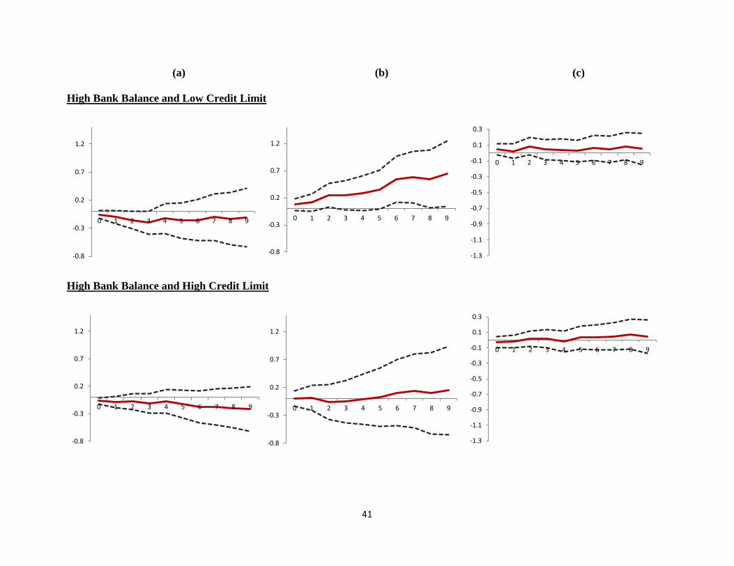
41
(a) (b) (c)
High Bank Balance and Low Credit Limit
High Bank Balance and High Credit Limit
-0.8
-0.3
0.2
0.7
1.2
0 1 2 3 4 5 6 7 8 9
-0.8
-0.3
0.2
0.7
1.2
0 1 2 3 4 5 6 7 8 9
-1.3
-1.1
-0.9
-0.7
-0.5
-0.3
-0.1
0.1
0.3
0 1 2 3 4 5 6 7 8 9
-0.8
-0.3
0.2
0.7
1.2
0 1 2 3 4 5 6 7 8 9
-0.8
-0.3
0.2
0.7
1.2
0 1 2 3 4 5 6 7 8 9
-1.3
-1.1
-0.9
-0.7
-0.5
-0.3
-0.1
0.1
0.3
0 1 2 3 4 5 6 7 8 9

42
Table 1: Summary Statistics This table reports the summary statistics of our treatment and control sample, both before and after propensity score
matching. The treatment sample consists of individuals who qualify for the Growth Dividend Program (but not for
other stimulus packages such as the Workfare Special Bonus), and the control sample consists of all
non-Singaporeans, as they do not qualify for the Growth Dividend Program. We also exclude individuals/accounts
that are dormant or closed or that had no transaction activity during the six-month period before the policy
announcement. Panel A shows the comparison of demographics between the treatment and control groups, both
before and after propensity score matching. Panel B shows the comparison of credit card and debit card spending,
credit card debt, and bank checking account balance information between the treatment and control groups in the
24-month sample period (2010:04–2012:03), both before and after propensity score matching. $benefit is the
Growth Dividend amount individuals received in the treatment group. Credit card spending is computed by adding
monthly spending over all credit card accounts for each individual. Credit card debt is computed as the difference
between the current month’s credit card payment and the previous month’s credit card balance. Credit card cycle
payment is the payment to the most recent credit card statement. Debit card spending is computed by adding
monthly spending over all debit card accounts for each individual. For the checking account, we compute # debit
transactions as the aggregate number of debit (outflow) transactions for each individual every month. # ATM debit
transactions/# branch debit transactions/# online debit transactions are the number of debit transactions at ATMs,
in branches, or via online transactions, respectively. Total card spending is the sum of debit card spending and credit
card spending for each individual in a month. All the dollar amounts are in the local currency (SG$), and 1SGD =
0.78 USD as of February 2011.
Panel A: Demographics of Treatment and Control Group
(1) (2) (3) (4) (5)
Mean Std. Mean Std.
Treatment Group Control Group Diff
Age 44.09 10.57 40.31 8.45 -3.78***
Monthly Income in 2010 6,053 8,861 7,795 11,395 1,742***
Female 0.42 0.49 0.30 0.46 -0.13***
Ethnicity
Chinese 0.89 0.31 0.49 0.50 -0.40***
Malay 0.05 0.22 0.01 0.07 -0.04***
Indian 0.03 0.18 0.17 0.38 0.14***
Married 0.47 0.50 0.49 0.50 0.02***
Property Type = HDB 0.70 0.46 0.55 0.50 -0.14***
$benefit 522 213 0 0
N 82,533 23,268
Matched Treatment Group Matched Control Group Diff
Age 40.37 8.87 39.57 8.00 -0.79***
Monthly Income in 2010 6,644 9,618 6,684 9,893 40
Female 0.38 0.49 0.35 0.48 -0.04***
Ethnicity
Chinese 0.88 0.33 0.76 0.43 -0.12***
Malay 0.003 0.06 0.003 0.06 0.00
Indian 0.07 0.26 0.13 0.34 0.06***
Married 0.45 0.50 0.45 0.50 -0.00
Property Type = HDB 0.66 0.47 0.65 0.48 -0.01
$benefit 511 214 0 0
N 36,989 10,567

43
Panel B: Financial Account Information of Treatment and Control Groups
(1) (2) (3) (4) (5) (6) (7) (8)
Treatment Group Control Group
Matched
Treatment Group
Matched
Control Group
Mean Std. Mean Std. Mean Std. Mean Std.
Credit Card
spending 721 1,183 1,047 1,644 763 1,229 824 1,343
cycle payment 701 17,193 1,043 2,485 736 6,258 798 1,843
debt 719 1,958 843 2,268 667 1,921 655 1,945
change in debt 6 490 7 652 6 514 4 551
Debit Card
spending 216 507 235 542 225 519 190 476
Bank Checking Account
# debit transactions 15 12 16 11 15 12 12 10
# ATM debit transactions 0.68 3.08 0.63 2.58 0.55 2.68 0.44 2.19
# branch debit transactions 0.32 0.88 0.27 0.74 0.28 0.81 0.24 0.71
# online debit transactions 0.26 0.71 0.29 0.72 0.32 0.78 0.30 0.73
month-end balance 16,036 21,823 14,320 20,531 15,513 21,391 14,083 20,076
Total (card) spending 937 1,290 1,282 1,770 988 1,341 1,014 1,443
total spending on transportation 77 130 44 89 78 129 44 91
total spending on dining 66 194 113 292 74 206 79 230
total spending on supermarket 56 119 95 181 59 122 67 144
total spending on apparel 86 246 131 316 93 256 100 270
total spending on travel 56 306 142 482 60 317 95 384
total spending on entertainment 38 154 37 120 36 142 28 106
N 1,893,217 512,213 845,339 233,197

44
Table 2: The Average Spending and Debt Response to the Stimulus Program
This table shows the average spending and debt response (Equations (1) and (2)) of the matched sample in the
period from 2010:08 to 2011:11. Panel A presents the estimation results of Equation (1), and Panel B shows the
estimation results of Equation (2). is the amount of the Growth Dividend received for the treatment
group, and is equal to zero for the control group. is a binary variable equal to one for the months after the
announcement of the Growth Dividend Program (i.e., later than 2011:01). is a binary variable equal to
one for the months during the announcement window (2011:02–2011:03), and is a binary variable equal
to one for the months after the disbursement of the Growth Dividends (i.e., later than 2011:04). Please refer to Table
1 for definitions of other variables. Individual and year-month fixed effects are included, and standard errors are
clustered at the individual level. T-statistics are reported in parentheses under the coefficient estimates, and ***, **,
and * denote statistical significance at the 1%, 5%, and 10% level, respectively.
Panel A
(1) (2) (3) (4)
Total card
spending
Debit card
spending
Credit card
spending
Credit debt
change
$ Benefit x 0.089*** 0.022*** 0.067*** -0.011*
(5.16) (2.65) (4.54) (-1.85)
Constant 1,204.544*** 490.356*** 714.188*** 16.206***
(164.56) (144.22) (111.65) (4.10)
R-squared 0.506 0.499 0.481 0.032
Panel B
$ Benefit x 0.080*** 0.009 0.071*** -0.011
(3.47) (0.82) (3.62) (-0.92)
$ Benefit x 0.092*** 0.026*** 0.066*** -0.011*
(4.93) (2.83) (4.15) (-1.85)
Constant 1,204.545*** 490.357*** 714.188*** 16.206***
(164.55) (144.22) (111.65) (4.10)
Fixed Effects Individual, year-month
R-squared 0.506 0.499 0.481 0.032

45
Table 3: Spending Response: The Number of Checking Account Debit Transactions
This table studies whether the number of checking account debit transactions change for the treatment group after the announcement of the stimulus program in
the matched sample during the period of 2010:08–2011:11. The dependent variables are the log of the number of debit, ATM debit, online debit, and branch debit
transactions (equal to ln(0.01) for zero values). Individual and year-month fixed effects are included, and standard errors are clustered at the individual level.
T-statistics are reported in parentheses under the coefficient estimates, and ***, **, and * denote statistical significance at the 1%, 5%, and 10% level,
respectively.
(1) (2) (3) (4)
# of debit transactions # of ATM transactions # of online transactions # of branch transactions
-0.000 -0.002 -0.013 0.006
(-0.04) (-0.28) (-0.85) (0.39)
Constant 2.660*** -4.224*** -3.803*** -4.026***
(914.29) (-1,228.81) (-441.63) (-385.52)
Fixed Effects Individual, year-month

46
Table 4: The Average Spending Response: Selected Categories of Spending
This table shows the average spending response (Equations (1) and (2)) by spending categories for the matched sample in the period of 2010:08–2011:11. The
dependent variable is the monthly total card spending on supermarket, dining, entertainment, transportation, apparel, and travel for each individual in our sample.
Panel A uses the dollar total spending as the dependent variable, and Panel B uses the log of total card spending as the dependent variable. Please refer to Tables
1 and 2 for definitions of other variables. Individual and year-month fixed effects are included, and standard errors are clustered at the individual level.
T-statistics are reported in parentheses under the coefficient estimates, and ***, **, and * denote statistical significance at the 1%, 5%, and 10% level,
respectively.
(1) (2) (3) (4) (5) (6)
Supermarket Dining Entertainment Transportation Apparel Travel
Panel A
$ benefit x 0.004** 0.002 0.002 0.003** 0.016*** 0.017***
(2.08) (0.68) (0.99) (2.40) (4.52) (3.66)
Constant 99.988*** 69.271*** 55.687*** 71.265*** 112.633*** 81.803***
(140.91) (67.45) (70.96) (178.79) (77.25) (33.59)
R-squared 0.588 0.479 0.699 0.797 0.407 0.253
Panel B
0.015 0.000 0.111*** 0.076** 0.135*** 0.088***
(0.41) (0.01) (3.09) (2.18) (3.32) (2.68)
Constant 1.512*** -1.346*** -1.982*** 1.056*** 0.339*** -3.498***
(64.20) (-56.64) (-91.78) (53.30) (12.54) (-173.16)
R-squared 0.588 0.479 0.699 0.797 0.407 0.253
Fixed Effects Individual, year-month

47
Table 5: Dynamics of Spending and Debt Response
This table reports the result of the estimation of the distributed lag model as in Equation (3) in the matched sample in the period of 2010:08–2011:11. is
a binary variable that is equal to one for the jth month after the announcement of the Growth Dividend Program. For example, is equal to one for the
announcement month (2011:02), and is equal to one for the 9th
month after the announcement (2011:11). Please refer to Tables 1 and 2 for definitions
of other variables. Individual and year-month fixed effects are included, and standard errors are clustered at the individual level. T-statistics are reported in
parentheses under the coefficient estimates, and ***, **, and * denote statistical significance at the 1%, 5%, and 10% level, respectively.
(1) (2) (3) (4)
Total card spending Debit card spending Credit card spending Credit debt change
$ Benefit x 0.062** -0.006 0.068*** 0.005
(2.19) (-0.44) (2.84) (0.26)
$ Benefit x 0.099*** 0.024* 0.074*** -0.026
(3.30) (1.68) (2.92) (-1.64)
$ Benefit x 0.152*** 0.052*** 0.100*** -0.037**
(5.19) (3.44) (4.10) (-2.32)
$ Benefit x 0.071** 0.046*** 0.025 -0.026*
(2.28) (2.90) (0.96) (-1.69)
$ Benefit x 0.057* 0.037** 0.020 -0.014
(1.83) (2.40) (0.74) (-0.94)
$ Benefit x 0.090*** 0.033** 0.057** -0.020
(2.87) (2.08) (2.12) (-1.28)
$ Benefit x 0.111*** 0.012 0.099*** 0.010
(3.52) (0.81) (3.65) (0.65)
$ Benefit x 0.137*** 0.035** 0.102*** -0.022
(4.31) (2.24) (3.74) (-1.43)
$ Benefit x 0.046 -0.007 0.053* 0.032**
(1.42) (-0.46) (1.93) (2.02)
$ Benefit x 0.065* -0.007 0.072** -0.009
(1.89) (-0.40) (2.46) (-0.54)
Constant 1,204.544*** 490.357*** 714.187*** 16.206***
(164.55) (144.22) (111.65) (4.10)
Fixed Effects Individual, year-month
R-squared 0.506 0.499 0.481 0.032

48
Table 6: Average Spending and Debt Response: Entire Sample, without Propensity Score
Matching
This table shows the results of average spending and debt response (Equations (1) and (2)) for the full sample
(without propensity score matching) in the period of 2010:08–2011:11. Panel A presents the estimation results of
Equation (1), and Panel B shows the estimation results of Equation (2). Please refer to Table 1 and 2 for definitions
of other variables. Individual and year-month fixed effects are included, and standard errors are clustered at the
individual level. T-statistics are reported in parentheses under the coefficient estimates, and ***, **, and * denote
statistical significance at the 1%, 5%, and 10% level, respectively.
Panel A
(1) (2) (3) (4)
Total card
spending
Debit card
spending
Credit card
spending
Credit debt
change
$ Benefit x 0.046*** 0.016*** 0.030*** -0.003
(3.80) (2.73) (2.92) (-0.76)
Constant 1,228.324*** 507.068*** 721.257*** 17.729***
(249.32) (219.85) (168.50) (6.73)
R-squared 0.546 0.513 0.524 0.035
Panel B
$ Benefit x 0.085*** 0.014* 0.071*** 0.003
(5.33) (1.88) (5.16) (0.42)
$ Benefit x 0.035*** 0.016** 0.019* -0.005
(2.71) (2.57) (1.72) (-1.17)
Constant 1,228.318*** 507.068*** 721.250*** 17.727***
(249.32) (219.85) (168.50) (6.73)
R-squared 0.546 0.513 0.524 0.035
Fixed Effects Individual, year-month

1
APPENDIX
Table A1: Payout Schedule of the Growth Dividend Program in 2011
This table summarizes the payout schedule of the Growth Dividend Program by income and annual value of
residence. We do not directly observe the annual value of residence, which is determined by IRAS, Singapore’s tax
authority, but we make use of the fact that the SG$13,000 cutoff is chosen to identify Singaporeans who live in
government subsidized housing (HDB). Singaporeans living in HDB can have different Growth Dividends,
especially among the lower income individuals. For our purposes, we use the average of the two dividend values for
individuals living in HDB within the same income category. For example, for Singaporeans with an annual income
no greater than SG$30,000, if they live in HDB, we assign them a Growth Dividend of SG$700. The exchange rate
in February 2011 was 1 SGD = 0.78 USD.
Assessable Annual Income in 2010 Annual Value of Residence (as of December 2010)
<= SG$7,000 SG$7,001 to SG$13,000 > SG$13,000
HDB Non-HDB
<= SG$30,000 SG$800 SG$600 SG$300
SG$30,001 to SG$100,000 SG$600 SG$600 SG$300
>SG$100,000 SG$100
National Service Men +SG$100

2
Table A2: Propensity Score Matching Logistic Regression
This table presents the results of the propensity score matching logistic regression. The dependent variable, eligible,
is equal to one for individuals in the treatment group, and zero for those in the control group. The treatment sample
consists of individuals who qualify for the Growth Dividend Program (but not for other stimulus packages such as
the Workfare Special Bonus), and the control sample consists of all non-Singaporeans, as they do not qualify for the
Growth Dividend Program. We also exclude individuals/accounts that were dormant or closed or that had had no
transaction activity during the six-month period before the policy announcement. In addition to the explanatory
variables below, we include 16 occupation categories as fixed effects. T-statistics are presented in parentheses below
the coefficient estimates, and ***, **, * represent statistical significance at the 1%, 5%, and 10% level, respectively.
(1)
Eligible
ln(age) -2.106***
(-4.48)
ln(monthly income in 2010 -2.322***
(-11.24)
ln(age) x ln(monthly income in 2010) 0.550***
(9.91)
property type dummy (HDB=1) 0.350***
(16.66)
Chinese 3.106***
(104.28)
Malay 4.718***
(48.00)
Indian 1.090***
(28.30)
married -0.066***
(-3.28)
female 0.357***
(17.72)
Fixed Effects Occupation
Constant 8.795***
(5.04)
Observations 103,985
Pseudo R-squared 0.265