consumer myopia, imperfect competition and the energy
TRANSCRIPT

François Cohen, Matthieu Glachant and Magnus Söderberg
Consumer myopia, imperfect competition and the energy efficiency gap: evidence from the UK refrigerator market Article (Accepted version) Refereed
Original citation: Cohen, François, Glachant, Matthieu and Söderberg, Magnus (2017) Consumer myopia, imperfect competition and the energy efficiency gap: evidence from the UK refrigerator market. European Economic Review . ISSN 0014-2921 DOI: 10.1016/j.euroecorev.2017.01.004 Reuse of this item is permitted through licensing under the Creative Commons:
© 2017 Elsevier B.V. CC BY-NC-ND 4.0
This version available at: http://eprints.lse.ac.uk/69188/ Available in LSE Research Online: February 2017
LSE has developed LSE Research Online so that users may access research output of the School. Copyright © and Moral Rights for the papers on this site are retained by the individual authors and/or other copyright owners. You may freely distribute the URL (http://eprints.lse.ac.uk) of the LSE Research Online website.
brought to you by COREView metadata, citation and similar papers at core.ac.uk
provided by LSE Research Online

Accepted Manuscript
Consumer Myopia, Imperfect Competition and the Energy EfficiencyGap: Evidence from the UK Refrigerator Market
Francois Cohen , Matthieu Glachant , Magnus Soderberg
PII: S0014-2921(17)30010-7DOI: 10.1016/j.euroecorev.2017.01.004Reference: EER 2948
To appear in: European Economic Review
Received date: 19 May 2016Accepted date: 4 January 2017
Please cite this article as: Francois Cohen , Matthieu Glachant , Magnus Soderberg , Consumer My-opia, Imperfect Competition and the Energy Efficiency Gap: Evidence from the UK Refrigerator Market,European Economic Review (2017), doi: 10.1016/j.euroecorev.2017.01.004
This is a PDF file of an unedited manuscript that has been accepted for publication. As a serviceto our customers we are providing this early version of the manuscript. The manuscript will undergocopyediting, typesetting, and review of the resulting proof before it is published in its final form. Pleasenote that during the production process errors may be discovered which could affect the content, andall legal disclaimers that apply to the journal pertain.

ACCEPTED MANUSCRIPT
ACCEPTED MANUSCRIP
T
1
Consumer Myopia, Imperfect Competition and the
Energy Efficiency Gap: Evidence from the UK
Refrigerator Market
This version: November 2016
François Cohen, London School of Economics and Political Science, London,
UK
Matthieu Glachant, MINES ParisTech and PSL – Research University, Paris,
France*
Magnus Söderberg, University of Gothenburg, Sweden
Abstract
The empirical literature on the energy efficiency gap concentrates on demand
inefficiencies in the energy-using durables markets and finds evidence that
consumers underestimate future energy costs when purchasing a new
appliance. We take a broader view and also consider the impact of imperfect
competition. Using data on the UK refrigerator market (2002-2007), we find
that the average energy consumption of appliances sold during this period was
only 7.2% higher than what would have been observed under a scenario with a
perfectly competitive market and non-myopic consumers. One reason for this
small gap is that market power actually reduces energy use.
Keywords: Energy Efficiency; Electricity Prices; Consumer Myopia;
Imperfect Competition.
JEL Classification: D12, L68, Q41.
* Corresponding author: CERNA – Centre for industrial economics, MINES
ParisTech, 60, boulevard St Michel, 75006 Paris, France.
matthieu.glachant@mines-paristech

ACCEPTED MANUSCRIPT
ACCEPTED MANUSCRIP
T
2
1. Introduction
In energy and environmental policy circles, it is commonly believed that an
“energy efficiency gap” exists between the desirable level of energy
consumption and observed consumption (e.g. IEA 2007, Ryan et al. 2011).
Since the seminal paper by Hausman (1979) and the discussion of possible
policy implications by Jaffe and Stavins (1994), the energy efficiency gap has
also attracted considerable interest in the academic literature (see the literature
survey by Gillingham and Palmer 2014).
To clarify the notion, it is necessary to distinguish two reasons that drive the
gap between the actual and socially optimal levels of energy consumption. The
first is the classic externality problem: the production and consumption of
energy, in particular of fossil fuels, generate major environmental and health
externalities which could be mitigated by policies promoting energy
conservation. The energy efficiency gap refers to a second category of failures
in the markets of energy-using durables. Energy efficiency outcomes involve
decisions whereby consumers first make an upfront investment in durable
goods and then consume energy through their use. Examples include water
heaters, building insulation, motor vehicles and household appliances. The
idea of the gap is rooted in a widespread belief that the market for energy-
using durables does not operate effectively, i.e. markets are not perfectly
competitive with fully rational economic agents. As a result, the market
equilibrium maintains an energy efficiency gap defined as a wedge between
the cost-minimizing level of energy efficiency and the level actually reached.
Policy discussions, as well as the academic literature, focus on the demand-
side of the markets (IEA, 2007; Ryan et al., 2011; Allcott and Greenstone,
2012; Gillingham and Palmer, 2014). The key concern here is that imperfect
information and other cognitive constraints could lead consumers to discard

ACCEPTED MANUSCRIPT
ACCEPTED MANUSCRIP
T
3
privately profitable investments.1 More specifically, it is often asserted that
consumers are myopic in the sense that they give too much weight to the
upfront cost or, expressed differently, the discount rate implicitly used to
calculate the net present value of the investment is too high. As a result,
consumers use too much energy.
This is only half of the picture, however. On the supply side, manufacturers of
energy-using durables also make decisions. In particular, they choose product
characteristics and set the price at which products are sold. In the case of
household appliances, they have a great deal of influence as these markets
tend to be very concentrated. In 2011, Whirlpool Corporations, AB Electrolux,
General Electric Company, and LG Electronics represented 90% of the sales
of major household appliances in the US (Alegria et al., 2012). In the UK,
competition on the refrigerator market is seemingly more intense as the top 5
companies represent around 46% of sales in our data for each year of the study
period. However, product differentiation reduces competition as soon as we
look at specific categories of products. For example, if we consider
homogeneous segments of refrigerators or refrigerators-freezers that are either
built-in or freestanding and of a specific energy efficiency class, the top 5
represent around 67% of sales in each segment.
In this paper, we consider both the role of potential consumer myopia and
imperfect competition on energy consumption of refrigerators sold in the UK
market. We use annual product-level panel data from 2002 to 2007 to analyze
1 The nature of the underlying causes of demand inefficiencies is extensively discussed by
Gillingham and Palmer (2014). Most of these causes are related to imperfect information. The
simplest mechanism is when the decision-maker lacks information on the true benefits of
energy efficiency investments. However, principal-agent problems can also arise when one
party makes a decision related to energy use, and another party pays or benefits from that
decision. For example, the landlord may pay for heating, while the tenant chooses how much
energy to use. Another potential barrier is if the investor faces credit constraints that are
stronger than for other investments because the lender finds it difficult to evaluate the payoff
from energy-efficiency investments.

ACCEPTED MANUSCRIPT
ACCEPTED MANUSCRIP
T
4
two types of decisions: consumer purchase decisions and suppliers’ price-
setting decisions. Next, we use our estimates to identify counterfactual
scenarios with perfect competition and without consumer myopia. This gives
us an estimate of the size of the energy efficiency gap which is defined in this
paper as the difference between actual average energy consumption of sold
appliances and the hypothetical consumption that would be observed in a
perfectly competitive market with non-myopic consumers.
Our approach provides a more comprehensive measurement of the energy
efficiency gap than that available in the literature. As mentioned above,
existing works mostly concentrate on demand inefficiencies as illustrated by
the recent reviews by Allcott and Greenstone (2012) and Gillingham and
Palmer (2014). We go further, by examining the role of suppliers and
imperfect competition.2 We however limit ourselves to a study of the short-run
equilibrium, where suppliers only choose prices, once product characteristics
have been chosen. The impact of product innovation is left for future research.
We also do not deal with all the imperfections that may influence energy use.
In particular, we rule out any considerations related to the pricing of
environmental externalities related to energy production and use or principal-
agents problems3
Our contribution to the relevant empirical literature is
discussed in more detail in the next section.
2 The academic literature is reviewed in the subsequent section. Supply side aspects have been
studied for instance by Fischer (2005), Jacobsen (2013), Houde (2014a, 2014b), and Goldberg
(1998). In contrast with our paper, these studies do not seek to measure the size of the energy
efficiency gap. Rather they evaluate specific policy scenarios (e.g. standards, feebates, energy
labeling, etc.). A limited industrial organization literature has also examined the functioning of
appliance markets (e.g. Ashenfelter et al., 2103; Spurlock, 2014). 3 We also do not investigate how certain policies or regulations might alter the functioning of
the markets. As an illustration, trade barriers may have hindered the imports of non-EU
refrigerators during the study period. As appliances produced by well-known European brands
tend to be more energy efficient than non-EU brands, removing barriers would increase
energy use.

ACCEPTED MANUSCRIPT
ACCEPTED MANUSCRIP
T
5
Although there is no universal definition of the energy efficiency gap, we are
aware that our definition is not the most common, as we depart from the view
that limits the energy efficiency gap to consumer behavior. We are however
not the only scholars who integrate supply-side inefficiencies as a cause of the
wedge between actual and optimal energy use (for instance, see the papers by
Jaffe and Stavins (1994) or Gerarden et al. (2015)). One could question the
relevance of integrating both demand-side and supply-side inefficiencies in a
unified framework instead of studying these imperfections separately. Such a
global assessment is necessary if the purpose of measuring the energy
efficiency gap is to identify and justify desirable policy intervention, a point
made before us by Fischer (2005) and, more recently, by Gerarden et al.
(2015) who stress the importance of supply-side factors when designing
policies to promote energy-efficient household appliances. Take the example
of the subsidies on energy-efficient goods that are recommended by some
economists to mitigate demand inefficiencies (e.g. Allcott, Mullainathan, and
Taubinsky, 2014) and widely implemented in practice. If producers benefit
from lower markups on energy-efficient goods than on less efficient ones – as
is the case in the UK refrigerator market in this paper – then subsidies should
be lower than they would be if prices were equal to marginal costs.4
We model demand using a standard discrete choice model with differentiated
quality based on Berry (1994). We take the first-difference to eliminate time-
invariant product attributes. A nested logit framework is used to control for
product segmentation caused by product differentiation. To address
endogeneity issues arising from the simultaneous determination of refrigerator
prices and quantities, our instrumentation strategy incorporates data from two
outside product markets – freezers and washing machines – which present
4 Another option would be to adjust antitrust regulations, which is the primary policy tool to
mitigate imperfect competition concerns. However this tool was not initially conceived for
sector-specific adjustments.

ACCEPTED MANUSCRIPT
ACCEPTED MANUSCRIP
T
6
different demand characteristics but technical similarities that lead production
costs to be correlated. Choices made by suppliers in terms of prices and
products offered on the market are estimated using reduced-form equations
that impose few restrictions on how they compete on the market. More
specifically, the price equation is estimated with a fixed-effect model in which
shocks on market shares are used to identify the size of mark-ups. We identify
the model using instruments that exploit a well-known effect in the marketing
field, i.e. “extremeness aversion” (Simonson and Tversky, 1992), which
affects demand for specific goods in a way that is unrelated to product features
in absolute terms, and thus is not systematically correlated with production
costs.
What transpires from our estimates is that the impact of the two market
imperfections on energy consumption is limited. On the demand side, we find
that consumers underestimate future energy savings by 35% in our base
specification which assumes a financial discount rate of 4.6%. This suggests
investment inefficiencies of reasonable size, which is equivalent to applying
an implicit discount rate of 11% to the stream of future electricity costs when
calculating the net present value. In line with these numbers, our simulations
show that myopia increases energy use by only 9.2% compared to a scenario
in which consumers would correctly value future energy costs.
The impact of imperfect competition is also modest, but goes in the opposite
direction: it reduces energy use by 4.2% compared to a scenario with perfect
competition. The reason is that products that consume more energy have
higher market shares on average. Suppliers thus have more latitude to raise
their price, which reduces demand. This pattern is likely to be true in other
markets of energy-using consumer durables where competition is less intense
or demand elasticity is lower for energy-intensive models. As the two
imperfections exert opposite effects, the joint effect is a modest 7.2% increase
ACCEPTED MANUSCRIPT
ACCEPTED MANUSCRIP
T
7
in energy use compared to a perfectly competitive market with fully rational
consumers.
These simulations therefore suggest that there would be few energy savings to
expect from reaching a fully competitive market with non-myopic consumers.
Likewise, we show that consumer myopia and imperfect competition have
limited impact on social welfare (excluding environmental externalities, but
including consumer surplus and profits). Consumer surplus5 would increase by
around £76 per sale in the first best optimum – just under 26% of the price of
appliances – but most of this increase is a transfer from suppliers, as the
overall increase in social welfare is only £18.10. These numbers convey an
important message about public policies targeting the energy efficiency gap.
With the exception of energy labeling, which seems to have been sufficient to
mitigate imperfections in the UK refrigerator market, policies should primarily
be concerned with the traditional environmental externality problem.
The rest of the paper is structured as follows. In the second section, we briefly
review the literature and justify why refrigerators constitute a suitable case
study to investigate the functioning of durable goods markets. Section 3
develops the conceptual framework. Section 4 presents the data. Section 5
outlines our empirical strategy and addresses identification issues. Estimation
results are presented in Section 6. In Section 7, we run simulations to predict
the impacts on the energy consumption of sold appliances and evaluate the
welfare impacts of imperfect competition and consumer myopia. Section 8
summarizes our findings and formulates policy implications.
5 Note that consumer surplus includes the utility that consumers derive from the other non-
energy related attributes of the products they purchase.

ACCEPTED MANUSCRIPT
ACCEPTED MANUSCRIP
T
8
2. Related literature
The empirical literature on the energy efficiency gap in the residential sector is
well developed. As explained above, the majority of existing papers focus on
demand and consumer myopia. Following the work of Hausman (1979) on
room air conditioners, early research found implicit discount rates that are
substantially larger than real financial discount rates. In the case of
refrigerators, the reported rates range from 39% to 300% (Revelt and Train,
1998; McRae, 1985; Meier and Whittier, 1983; Gately, 1980). More recent
studies have suggested lower rates. For refrigerators, Tsvetanov and Segerson
(2014) find discount rates in the 13-22% range in a study that looks at the
impact of energy labeling on consumer surplus. The same pattern is found in
recent papers dealing with gasoline prices and fuel efficiency. Allcott and
Wozny (2014), whose methodological approach is similar to ours, find a
discount rate of 16%. Busse et al. (2013) produce several estimates under
different assumptions, none of which exceed 20% and many of which are
close to zero. The same pattern is found by Goldberg (1998).
There are several reasons that explain why recent works, including ours, find
lower discount rates than earlier studies. The most important reason is the use
of panel data, which allows better control of unobserved product
characteristics. Indeed, using a hedonic pricing model on a cross section of
products as done by Hausman (1979), we find a discount rate of 210% (shown
in online Appendix K). Another reason may also relate to the fact that
consumers are better informed. For example, energy labeling has been
mandatory in the European Union for many appliances, including
refrigerators, since 1995. In the US and in Canada, the “Energy Star” label is
increasingly used.
As mentioned in the introduction, the main contribution of this paper is to
examine the potential influence of suppliers on the energy efficiency gap. A
few empirical papers also look at the supply side of energy-consuming

ACCEPTED MANUSCRIPT
ACCEPTED MANUSCRIP
T
9
durables markets. However, their question is different as they evaluate the
impact of a particular policy: fuel efficiency standards (Goldberg, 1998;
Jacobsen, 2013), feebates (e.g., d’Hautfeuille et al., 2013), energy labeling
(Houde, 2014a, 2014b), and fuel taxes (Verboven, 2002).
Refrigerators constitute a suitable case to explore these questions for reasons
that are best explained through a comparison with motor vehicles, for which
the impact of gasoline prices has been studied in several recent studies (e.g.,
Allcott and Wozny, 2014; Busse et al., 2013, Anderson et al., 2013). To start
with, and in contrast to car owners, who vary their usage intensity, refrigerator
owners cannot adjust energy consumption after purchase. As a result, future
energy consumption is exogenously determined by the characteristics of the
product. This suppresses an important source of bias and measurement errors.
A second advantage is that there is no market for used cold appliances. This is
obviously not the case for cars, and empirical analysis therefore needs to
develop complex solutions and/or make several assumptions to deal with this
issue. See for instance Jacobsen (2013), Li et al. (2009) or Allcott and Wozny
(2014). Third, the product is simple compared to cars and less influenced by
subjective feelings. This is a major benefit, as dealing with taste shocks and
unobserved product characteristics that tend to be correlated with energy
performance is a major methodological obstacle, particularly when using
market-level data, as done in this paper and many others.
3. Conceptual framework
In this section, we propose a framework including two components. First, a
demand model describes consumer purchase behavior; it serves to measure the
size of consumer myopia. Second, a price model describes the pricing
ACCEPTED MANUSCRIPT
ACCEPTED MANUSCRIP
T
10
behavior of the suppliers; it aims to understand the impact of imperfect
competition on the market.6
3.1 Demand
We develop a simple discrete choice demand model of the refrigerator market
based on Berry (1994). T markets each represent the UK refrigerator market
during year t (with t = 1,…,T). For each market, we observe aggregate
quantities sold, average prices, and product characteristics for J refrigerator
models.
Consumers choose the product that maximizes utility. The indirect utility
function of consumer i purchasing a new refrigerator j in year t is equal to
where is the average utility and is consumer i’s
unobserved heterogeneity that captures deviation from the average. The
average utility is:7
( )
In this expression, captures the usage value of the refrigerator j over its
lifetime which depends on product characteristics such as size and whether the
refrigerator is built-in or freestanding. is the purchase price and is the
discounted electricity cost. has a negative impact on which is
proportional to , the marginal utility of money, and a parameter , which
6 The framework described hereafter is static. A dynamic framework would be useful if our
aim were to explain the timing of consumers’ purchase decisions, for instance like Rapson
(2014), who uses a dynamic model to understand the adoption of energy-efficient air
conditioning in the US, since purchase decisions can be delayed for several years. In contrast,
the date of purchase of a new refrigerator is mostly exogenous as they are typically replaced
immediately when they break down or when the kitchen is renovated (and renovation is not a
consequence of the decision to purchase a new refrigerator). This is why we have chosen a
static framework which reduces the need for instrumentation and imposes weaker
assumptions. 7 This form of the indirect utility can be derived from a quasi-linear utility function, which is
free of wealth effects. This is a reasonable assumption for refrigerators, which usually
represent a small fraction of individual income.

ACCEPTED MANUSCRIPT
ACCEPTED MANUSCRIP
T
11
captures consumers’ perceptions of energy costs. If consumers are perfectly
rational, we obtain . If they are myopic, it is expected that they
underestimate the disutility from energy costs so that . Estimating this
parameter is a central objective of the paper.8
Next we decompose the value of usage in two additively separable terms:
where captures the time-varying component of the valuation
of observed and unobserved product characteristics. Hence, we get:
( )
Berry (1994) generalizes McFadden’s (1973) discrete-choice demand model
by transforming the logit model into a linear model that can be estimated with
aggregated market data. In Berry’s framework, the probability that good j is
purchased asymptotically corresponds to its market share at time t. Hence:
∑ ,
where denotes product j’s market share in year t. A consumer can also
choose the outside option, indexed 0, which represents the decision not to
purchase a refrigerator. Normalizing the utility of the outside option to
zero, the market share of product j at time t can be compared with the market
share of the outside good so that In logs, this simplifies to
( ) ( ) . This expression rests on the irrelevance of
independent alternatives (IIA) assumption that leads to biased estimates in
heterogeneous, segmented product markets.
8 Here, the modeling strategy is to adopt the standard rational choice model, except that we
include the parameter . An alternative approach would be to adopt a behavioral economics
framework, which is used by Segerson and Tsvetanov (2014). But this will prevent the
measurement of the energy efficiency gap, which is precisely the gap between actual behavior
and perfect rationality.
ACCEPTED MANUSCRIPT
ACCEPTED MANUSCRIP
T
12
To relax this assumption, we adopt a nested logit framework in which
consumers’ idiosyncratic preferences are correlated across refrigerators within
the same “nest” ( ( ) ), and zero otherwise.9 In this situation,
Berry shows that:
( ) ( ) ( ( ) ) ( ) ( )
where ( ) is the market share of product as a fraction of the total sales
within group g that includes product j and [ ] is a scalar that
parameterizes the within-nest correlations. Note that the model collapses to the
standard logit when .
In our base specification, we construct product groups based on three
dimensions that create product segmentation in the refrigerator market: a
capacity indicator that takes the value 1 when the capacity is above the sample
median capacity; an indicator that takes the value 1 when the appliance is a
combined refrigerator-freezer rather than a standard refrigerator; and an
indicator that distinguishes freestanding appliances from built-in ones. The
final model therefore includes 8 nests (2 x 2 x 2). This choice is based on our
belief that these three characteristics naturally divide the products into
different segments. A consumer purchasing a combined refrigerator-freezer
has a fundamentally different need than a consumer purchasing a standard
refrigerator. Similarly, the choice of size is strongly influenced by family
characteristics (size, food consumption habits, etc.) and dwelling
characteristics, whereas built-in refrigerators are more likely to be chosen by
consumers who are refurbishing their kitchen at the same time. In Appendix
9 Goldberg (1995) and Allcott and Wozny (2014) are other examples where the nested logit
model is used. A popular alternative is the random coefficient models. In this situation, the
nested logit model is suitable since it allows us to eliminate unobserved quality and cost
characteristics (such as exterior finish, electronic readouts, reliability, and automatic ice
makers) and the outside option through first-differencing. A random coefficient approach
requires us to quantify the outside option, which is uncertain and subject to measurement
errors.

ACCEPTED MANUSCRIPT
ACCEPTED MANUSCRIP
T
13
A, we run models with alternative nest structures and the results are not
qualitatively affected by different nests.
We now turn to the specification of the discounted lifetime electricity cost ,
which is our variable of interest. The parameter is inserted in Eq. (1) to
capture potential behavioral failures. As a consequence, should not be
viewed as the electricity cost perceived by real consumers, but rather the cost
they would consider if they were fully informed and rational. They would then
calculate the net present value of the electricity cost with the standard formula:
∑
( )
( )
In this equation, is product j’s lifetime, is the level of energy
consumption per time period,
is the electricity price at time that is
forecasted at the time of purchase and is the discount rate. As we consider
the behavior of a representative consumer,
, which is a national average
although actual prices can vary across locations. As a result, the variation in
the data comes from the interaction between model-specific and time-invariant
characteristics (i.e. lifetime and annual energy consumption) and time-varying
electricity prices. Note also that forecasted electricity prices are unobserved as
the data only include actual prices. They are estimated with an ARIMA model
that is described more fully in Section 4. We come back to these issues in
detail below.
3.2 Supply
In contrast to the demand equation, we adopt a reduced-form approach to
assess the impact of imperfect competition on prices. Previous empirical
contributions that examine supply-side issues (see the literature review above)
generally adopt a structural approach in which multi-product manufacturers
compete à la Bertrand. In the context of a nested logit model, Berry (1994)

ACCEPTED MANUSCRIPT
ACCEPTED MANUSCRIP
T
14
provides the formula applicable to compute equilibrium prices under Bertrand-
Nash competition:
( ) ( ) ( )
In this equation, is the unit production cost of model j at time t; and are
the parameters also included in the sales equation. As they can be estimated
with the demand equation, we could use (3) to directly compute the markups
without any additional estimation
However, this equation is likely to convey an incorrect estimation of the
markups. In practice, the markup values are heavily influenced by the choice
of nest structure (the smaller the nest, the higher the markup). As we lack
information to truly detect the real competitors of product j, the choice of nest
structure is arbitrary and therefore could very plausibly under- or over-
estimate competition intensity.10
More fundamentally, the Bertrand-Nash
setting overlooks the fact that this sector is characterized by the presence of
complex vertical relations between manufacturers and retailers, which also sell
refrigerators produced by other manufacturers under their own brand name.
A reduced-form approach copes neither with the issue of vertical relations nor
with the fact that nests may be wrongly specified, but is at least less reliant on
the strong assumption that the real competitors of product j are truly identified.
It thus provides a more flexible strategy to identify price margins.
Therefore, to avoid relying on specific assumptions about the structure of
competition, we consider that the purchase price is given by:
10 If we assume no nest at all (σ=0), we find an average markup of £ 119.8 with very little
variation across products (£ 119.7 – 120.4). With 8 nests as defined in the base model, the
sales-weighted average markup of all products used in the simulation falls to £ 21.6. The
lowest markup would be estimated at £ 21.4 and the highest at £ 28, with most products
having a markup close to the minimum.

ACCEPTED MANUSCRIPT
ACCEPTED MANUSCRIP
T
15
( ( ) )
In this equation, ( ) is a multiplicative term which captures the size of the
mark-up as a function of the product market shares and ( ) . The reader
may note that the choice of such a functional form relates to Berry’s formula
(3) since it includes the same determinants for the size of the markups.
However, it is less restrictive, as it does not include the parameters and
that are also present in the demand equation. The main difference with the
structural approach is then that additional assumptions will be made at the
simulation stage, that is, when using the econometric estimates to compute
e.g., the size of the energy efficiency gap. This makes it easier to check
whether they are valid, a point made by Busse, Knittel and Zettelmeyer (2013)
for instance. In this paper, these assumptions are presented in Section 7 where
we describe our simulations.
Taking logs and adopting a log linear specification for , the price equation
becomes:
( ) ( )
where is a product-fixed effect influencing the level of the mark-up and
( ) is the global market share of product 's nest in year . The log-log
functional form implies that a relative increase in market share is assumed to
have a constant relative impact on prices.
As mentioned above, this approach overlooks the long-run impact of imperfect
competition and consumer myopia on product characteristics and innovation.
In a preliminary stage of this research, we however applied a dynamic probit
model to our data in order to estimate product entry and exit. Results are
mostly similar to the ones obtained in the short run. The methodology and
results obtained are available on demand. However, this supplementary
analysis does not look at manufacturers’ capacity to reduce the cost of

ACCEPTED MANUSCRIPT
ACCEPTED MANUSCRIP
T
16
producing energy-efficient products in the long run. In the absence of cost
information, this question cannot be treated easily.
4. Data
We use market data from the refrigerator market in the UK on the product
level from 2002 to 2007 collected by the market research company GfK Retail
and Technology (received by the Department for Environment, Food and
Rural Affairs). The data includes detailed annual information on refrigerators
and combined refrigerator-freezers sold in the UK. We identify products by
brand name and series numbers. If not available, we rely on available
information on product features (width, height, total capacity, energy
consumption, energy efficiency rating, freestanding / built-in feature,
availability of no-frost system and of freezer). Note that products that are
similar in all respects but have a different brand name are considered to be
different. This is in line with the view that brand name is a product attribute
valued by consumers for itself. 11
Each observation is a product j in year t with measures including number of
units sold, average consumer price, and annual electricity consumption. We
also observe a set of product features such as size, whether it is a standard
refrigerator or a combined refrigerator-freezer, and indication of whether it has
a separate freezing compartment that can store food at -18°C. We do not have
information on product-specific lifetimes. Instead, we use the information
provided by the Association of Manufacturers of Domestic Appliances that
11 Brand name and series numbers were not available for store brands. For these products,
identification is based on product features alone. This means that, with this method, two
different store brand models with exactly the same product features cannot be properly
distinguished. Therefore, observations for store brand appliances are dropped each time the
same product corresponds to various models of appliances for the same year.

ACCEPTED MANUSCRIPT
ACCEPTED MANUSCRIP
T
17
estimates lifetimes of 12.8 years for refrigerators and 17.5 years for combined
refrigerator-freezers (AMDEA, 2008).12
A potential problem is that the data does not include information on energy
efficiency policies that may have influenced market outcomes. However, there
was no change in the design of the labeling scheme or in the strictness of the
regulatory standards during the sample period. Admittedly, the Energy
Efficiency Commitment (EEC) scheme was enforced during the study period,
offering eligible households the possibility of financial support for the
purchase of energy-efficient cold appliances. However, the measure had very
little impact on the refrigerator market. In practice, support mostly focused on
energy-efficient light bulbs and home insulation. Lees (2008) reports that
fridge-freezers subsidized by EEC represented 0.43% of the market between
2005 and 2008. If we also include subsidies from local authorities and the
Warm Front, subsidized appliances probably represented around 1.5% of all
cold appliances sold between 2005 and 2008.
We drop observations with low sales. In particular, we drop models where
annual sales never exceed 100 units over the study period. This ensures that
the models in the sample were actually commercialized on a large scale (not
only in a few local markets) during at least one year over the period. We also
drop observations (product-year) with less than 10 units sold to avoid having
models with sales near zero, which would make the estimation of the discrete
choice model unstable. Outliers are also dropped: we identify the 2.5% of
products with the highest and lowest prices, capacities and energy
12 The assumption that all appliances of a given type have the same lifetime disregards the fact
that some appliances may in fact have a longer/shorter expected lifetime. However, if
consumer expectations about lifetimes are constant over time, these cross-sectional differences
between appliances will be resolved when using either fixed effects or first differences to
estimate our econometric models. We furthermore show in the Appendix that changing the
lifetime of appliances when calculating operating costs has limited impacts on the estimated
parameters. This is because, on average, appliances have a long lifetime compared to the
implicit discount rate applied by consumers.

ACCEPTED MANUSCRIPT
ACCEPTED MANUSCRIP
T
18
consumptions, in addition to the 2.5% of products with the highest sales
levels. Any product falling within at least one of these categories is dropped
from the sample.13
Summary statistics on product characteristics are displayed in Table 1. The
data set used in the regressions includes 3,519 observations of which 2,265 are
used to construct the first differences for the econometric estimation of the
demand equation. The total number of differences used in the econometric
estimation is then 1,365. Descriptive statistics are based on the 2,265
observations used to construct the differences of the estimation sample of the
market share equation. Most appliances are larder fridges and fridge-freezers.
Although the data is not used in our estimation, we also know the product’s
classification according to the EU energy label. Energy labeling has been
mandatory since 1995 for all refrigerators sold in the European Union. In our
data, each product is assigned to a class from A++ (the most energy efficient)
to G (the least energy efficient). This rating does not capture the absolute
energy consumption of the appliance, but its relative consumption across
different classes. Table 2 provides an overview of the distribution of prices
and market shares across energy efficiency classes. Note that almost all
products were rated A, B or C during the study period.
13 Outliers in terms of price, capacity, energy consumption and sales are excluded for several
reasons. First, the data is reported to GfK and some observations appear to have been
miscoded. We want to remove from the data observations with absurd values. Second, we
exclude niche products, since they would not properly belong to the nests we have defined.
We also exclude best sellers because we do not observe commercialization strategies that can
be correlated with prices or energy efficiency and fear that these products have access to a
much wider web of providers than other goods. Tests have been run to check that our results
were not heavily dependent on how the sample was restricted.

ACCEPTED MANUSCRIPT
ACCEPTED MANUSCRIP
T
19
Table 1: Summary statistics on product characteristics
Variable Unit Mean Std
deviation
Annual sales, used for the log of market
shares ( )
# of units 1371.5 2251.6
Purchase price, real £ 394 246.7
Appliance lifetime, years 15.2
Energy consumption, kWh/year 306.3 136.5
Height cm 139.8 42.8
Width cm 59.3 9
Capacity liters 246.9 106.5
Energy efficiency ratinga 2.4 0.8
Share of combined refrigerators-freezers 0.51
Share of built-in appliances 0.74
Share of appliances with no-frost system 0.23
Notes. Source: GfK, provided by Defra. Survey years: 2002-2007. 2,265
observations. a To obtain a numeric value for the energy efficiency rating (from “G”
to “A++”), ratings were recoded with “A++” set equal to 0, “A+”=1, “A”=2 and so
on up to “E”=6. The data used in the regression does not comprise “F” and “G”
labeled products.
Table 2: Sales-weighted price and market share of appliances,
breakdowns by energy efficiency class
Energy efficiency rating Sales-weighted average price Market share
A++ 392.3 0.03%
A+ 294 3.38%
A 324.7 57.87%
B 267.3 25.82%
C 237.2 12.43%
D 313.6 0.48%
E 257 0.01%
Notes. Source: GfK, made available by Defra. Survey years: 2002-2007. 2,265
observations. No observation with energy efficiency rating of “F” or “G”.
The data also suggest the degree of imperfect competition prevalent in the
market. Restricting to 2007 for simplicity, the refrigerator market was
composed of 66 manufacturer brands, selling an average of 25 different
products each. A few brands concentrated most of the sales: the top 5 and top
10 manufacturers respectively commercialized 48% and 68% of all the

ACCEPTED MANUSCRIPT
ACCEPTED MANUSCRIP
T
20
products sold in that year. However, market shares of these top manufacturers
have a similar size, none of them exceeding 20%. As a result, the Hirschman-
Herfindhal Index (HHI) was around 770 at the global 2007 level, which does
not suggest strong market power.
These numbers however ignore the existence of product differentiation.
Refrigerators have radically different sizes and energy efficiency levels. They
can also include specific features, such as water and ice dispensers or free-
frost technology to make maintenance easier. Some consumers buy built-in
appliances to fit better in their kitchen whereas others opt for freestanding
appliances, etc. As a result, a given product actually has a fairly limited
number of direct competitors. We thus need to reassess the degree of
imperfect competition by calculating HHI for specific market segments. For
example, consider eight market segments of refrigerators or refrigerator-
freezers, that are either built-in or freestanding and either above or below the
median size. The HHI lies above 1,500 (moderate concentration) in 3 cases out
of 8. If we further breakdown the market based on the energy efficiency rating
of appliances, this produces a total of 37 sub-segments of refrigerators or
refrigerator-freezers that are either built-in or freestanding, of a comparable
size and with the same energy efficiency rating. The HHI is above 2,500 (high
concentration) in 23 of these sub-segments.
We now explain how we derive the electricity cost variable from the data.
Recall that:
∑
( )
As indicated earlier, should be viewed as the valuation of cost by a
sophisticated and informed decision-maker. This hypothetical consumer
knows the annual energy consumption ( ) and lifetime ( ) of each model

ACCEPTED MANUSCRIPT
ACCEPTED MANUSCRIP
T
21
available on the market. He considers the opportunity cost of capital when
determining the appropriate discount rate.
Choosing the value of is critical as it directly influences , and thus the
importance of consumer myopia. Consider first a consumer who purchases a
refrigerator from her/his savings. The opportunity cost is then related to the
return that could be made on these savings. More precisely, the discount rate
should equal the real average bond deposit rate of UK households (2.83%
according to the Bank of England for the period 2002-2007). Consider then a
consumer who buys on credit. Now her/his opportunity cost corresponds to the
average interest rate. A possible reference is the rate of credit card lending
(13.98% according to the Bank of England for the period 2002-2007).
Accordingly, the discount rate to be applied should be a weighted average of
both these rates where weights equal the share of both types of consumers. In
this study, we use statistics on method of payment for furniture available in the
UK food and expenditure survey. In 2007, 2.06% of respondents who
purchased furniture used a loan, 1.98% hired their product, 11.90% used a
credit card and the remaining 84.06% used cash or another method of
payment.14
Assuming the same patterns for refrigerators - products present
similarities, in particular, similar average prices, we have considered that the
proportion of consumers likely to use a credit card loan or a similar type of
loan for the purchase of a refrigerator is around 16%. Using this weight, we
find a discount rate r equal to 4.6%.
Measuring the forecasted electricity price
is more problematic as we only
observe real electricity prices. Furthermore, there was a drastic surge in
electricity prices in the UK over the period, implying that observed and
expected electricity prices could very well differ. As a benchmark, we
14 The survey does not describe these other methods, which would include, to our
understanding, debit cards and cheques.

ACCEPTED MANUSCRIPT
ACCEPTED MANUSCRIP
T
22
consider that a perfectly rational consumer calculates future electricity prices
based on the entire series of past prices. We approximate this calculation
process by an autoregressive integrated moving-average model (ARIMA) on
monthly data of real electricity prices. This technique allows us to recreate the
entire flow of future expected electricity prices that enter Eq. (2). The best fit
with our data is obtained with an ARIMA process with one lag for the
autoregressive term and one lag for the moving-average term:
where , and are parameters and is the error term at time t. The model
is used recurrently to make forecasts, using predictions of the previous periods
to calculate new predictions. We re-estimate this model for each year to allow
decision-makers to use all of the data that are observed at each time period.
This implies that the model is updated each year based on previous market
data; e.g. the price expectations for consumers in 2003 are based on prices up
until Dec. 2002). We then calculate the forecasted prices as:
( )
where and are estimates of and using all the data available on
electricity prices up to time t. The detailed results of the ARIMA models are in
Appendix C.
In online Appendix M, we also develop an alternative approach in which
forecasts are derived from the futures prices in the wholesale electricity
market. The intuition for this approach is that the futures market aggregate
information on future prices initially owned by sophisticated market
participants. These results are similar to the ones we obtain when using the
ARIMA model. Another alternative would be to proxy the forecasted
electricity price by its current price. In a recent paper, Anderson et al. (2013)
show that US consumers tend to believe that gasoline prices follow a random
walk, so that the current price is a martingale. However, this approach is not

ACCEPTED MANUSCRIPT
ACCEPTED MANUSCRIP
T
23
consistent with the assumption we make, since we do not want to capture
real-world expectations, but rather to describe cost valuation by a
sophisticated decision-maker so that the parameter only captures the size of
the deviation from this benchmark.15
Figure 1 presents the real monthly electricity price data, which is calculated
using data on retail electricity prices from the Department of Energy and
Climate Change (DECC, 2013a).
Figure 1: Average monthly electricity prices in the UK, 1996-2014
Note: Prices in pence per kWh with CPI=1 in 2005. The study period is between the
two vertical lines.
Note also that the study period 2002-2007 is marked by a dramatic rise in the
electricity price driven by increasing gas prices (about 8% per year) after a
period of decreases pre-2002. Consequently, forecasts are consistently below
actual prices during the period, i.e. an error that decreases the size of .
15 We do, however, provide the results under this assumption in online Appendix M as a test
of robustness. This leads to an increase of the size of γ (and thus reduces myopia).
810
12
14
2005 p
ence p
er
kW
h
1996 1998 2000 2002 2004 2006 2008 2010 2012 2014

ACCEPTED MANUSCRIPT
ACCEPTED MANUSCRIP
T
24
5. Estimation
In this section, we specify the different equations and discuss identification
issues.
5.1 Demand
To derive an econometric specification for short-term sales, we first add year
dummies to eq. (1) to eliminate the share of the outside option and any shift
in the overall market share level. Next we take the first-difference in order to
eliminate the value of usage.16
This leads to:
( ) ( ) ( ( ) ) ( )
where is the first-difference operator and is the econometric error term
capturing unobserved time- and product-varying heterogeneity.
A concern with Eq. (6) is that the purchase price is endogenous since
quantities and prices are simultaneously determined in market equilibrium.
The origin of this problem is that unobserved time-varying product
characteristics affect both consumers’ product valuation and prices, i.e.
[ ] . The log of the within-nest market share ( ( ) ) is also
endogenous. A higher value of increases the sales of refrigerator and
because this product belongs to nest , an increase in mechanically
increases ( ) . An instrumental variable approach is therefore adopted.
Another reason for doing so is to circumvent potential measurement errors in
the price variable since we do not observe transaction prices but a national
16 We use first-differencing instead of demeaning since this allows us to directly estimate and
in a non-linear GMM estimation. A first-differencing is only efficient when there is no serial
correlation. When testing for serial correlation in the first-differenced model using a
Wooldridge test, we find evidence of serial correlation. We account for serial correlation in
the estimation of the standard errors using clustered robust standard errors at the product level.
A fixed effect specification in level is displayed in online Appendix I. The estimated
coefficients in the first-differenced and fixed effects models are comparable in size and not
statistically different from each other.

ACCEPTED MANUSCRIPT
ACCEPTED MANUSCRIP
T
25
average transaction price calculated by GfK.17
Applying a valid instrument on
prices addresses de facto the attenuation bias caused by measurement errors.
A common instrumentation approach in industrial organization is to take
advantage of the fact that the market is imperfectly competitive. In such
situations it is claimed that non-price characteristics of products
influence but not the utility . Berry (1994) suggests using the nest
structure of the model. His proposed instruments are the averages for different
product features within and/or out of the nest that product j belongs to. This
approach is extended in Berry et al. (1995) and has been adopted in many
studies.
A weakness of this strategy is that taste shocks that affect other products can
also influence the utility of product . For instance, marketing efforts by a firm
can induce a taste shock that affects all of its products, or given characteristics
that concern several models might become popular among consumers. The
fact that refrigerators are quite standardized products, except in the dimensions
we base the nests on, is not necessarily advantageous when instrumenting with
other products’ characteristics. This means that unobserved product
characteristics are likely to be correlated across nests and manufacturers.
Significant standardization also implies that product characteristics may not
evolve sharply over time and therefore that within and outside nest averages
they may remain stable from one year to the next, reducing the strength of
potential instruments. We indeed find that when we use instruments of this
type, they are weak (shown in online Appendix L).
This leads us to adopt an alternative approach where instruments are related to
the price of products sold in two related markets: the upright freezer market
(i.e. excluding the chest freezer market) and the washing machine market.
17 This problem is likely to be less severe than in the automobile market, where list prices can
widely diverge from the prices that are actually paid after commercial negotiations.
ACCEPTED MANUSCRIPT
ACCEPTED MANUSCRIP
T
26
Freezers and washing machines present two useful characteristics. First, they
are sold outside the refrigerator market, and thus to different consumers. This
implies that taste shocks are less likely to be correlated with those observed in
the refrigerator market. Second, they share some technical similarities with
refrigerators as they are all large household appliances. This means that shocks
affecting production costs – e.g., an increase in steel prices – are likely to be
correlated across these markets. The prices of freezers and washing machines
are therefore likely to be correlated with cost shocks in the refrigerator market.
This approach presents some similarities with the strategy implemented by
Hausman et al. (1994), which uses prices of the same product in other regions
(and thus in different markets) as instruments. We use the price of similar
products in other markets. The common identification assumption is that
prices in outside markets reflect underlying product costs and stochastic
market-specific factors that are independent from those observed in the fridge
markets.
The difficulty with this approach is to match outside prices to the price of a
specific refrigerator, as goods are different. Our solution is to use two product
characteristics that are common to refrigerators, freezers, and washing
machines, i.e. capacity and whether the appliance is built-in or freestanding.
Using a hedonic pricing model, we estimate a year-specific implicit price for
these two characteristics on product-level data for the UK freezer and washing
machine markets between 2002 and 2007 obtained from GfK. This gives a
year-specific average for subcategories of freezers and washing machines,
which we match with the same subcategories of refrigerators-freezers and
refrigerators. For example, the implicit price of smaller than average built-in
freezers at time t is used as an instrument for the price of smaller than average,
built-in refrigerators and refrigerator-freezers at time t. Importantly, we
include brand-specific time trends in the hedonic pricing model in order to
control for changes in brand-specific marketing strategies and image. This
ensures that variations in the hedonic prices of the two characteristics do not

ACCEPTED MANUSCRIPT
ACCEPTED MANUSCRIP
T
27
capture changes in brand image, which could be correlated with the sales of
refrigerators with the same brand name. To ensure that our estimation is not
biased by changes in the retail sector, trade brand products have been
withdrawn from the sample used to estimate the implicit price of the two
attributes. All the details of how these instruments are constructed are included
in Appendix B.
As previously evoked, another issue is that, as data on refrigerators are only
available at the national level, we use the national average electricity price to
compute . This potentially creates a measurement problem, as the price of
electricity may be different across regions. However, regional price
heterogeneity is likely to be modest. In 2013, statistics show that regional
differences are within ±5% of the national average, except for Northern
Ireland where less than 3% of the UK population resides. Measurement errors
may also arise for two other reasons. First, we have averaged the interest rate
on credit card loans and the deposit rate for fixed bound deposits to compute
the discount rate. Second, consumer heterogeneity (e.g. in terms of
environmental awareness) may lead some consumers to prefer energy-efficient
appliances. The sorting of consumers across products (as in Bento, Li and
Roth, 2012) would imply that product-specific energy costs are measured with
errors and thus endogenous. In Appendix E, we give results with a
specification whereby the operating cost is instrumented with its lagged values
to control for all potential measurement problems. We find small differences.
A final issue is that we only have access to the average UK electricity prices,
whereas perfectly rational consumers are unlikely to care about average prices,
but only consider marginal prices. The results of our base model are not biased
provided that the level of the fixed part of the tariff did not change between
2002 and 2007, which is plausible as the rise was driven by gas price increases
that raised the (variable) cost of electricity generation. However, in Appendix

ACCEPTED MANUSCRIPT
ACCEPTED MANUSCRIP
T
28
D we run a robustness test where we assume that the share (not the level) of
the fixed part remains stable. This slightly inflates the size of .
5.2 Supply
For convenience, we rewrite Eq. (4) here
( )
To deal with the problem that the production cost is not observed, we assume
that ( ) ( ) where is a product fixed effect,
( ) , a by-brand by-year fixed effects, and ( ) , a by-year by-nest fixed
effect. captures time-varying shocks on the production cost. Introducing
these different fixed effects will absorb the terms and . As a result,
and slightly abusing notations, the price equation is now:
( ) ( ) ( ) ( ) ( )
The multiple fixed effects allow controlling for most unobserved factors that
influence cost. However, there is a price to be paid: It is not possible to
estimate the value of and econometrically, and thus to directly infer the
size of the markup from these estimates. When performing the simulations, we
therefore bypass the obstacle using external information on average markups
in the UK cold appliance industry.
Obviously, ( ) is endogenous in Eq. (7) for the same reason that was
endogenous in the sales equation. But we now need an instrument that is
correlated with demand shocks but uncorrelated with costs. Our strategy relies
on a well-known effect in the marketing field, i.e. the “compromise effect”
(Drolet, Simonson and Tversky, 2002) or “extremeness aversion” (Simonson
and Tversky, 1992). This says that demand for differentiated goods is affected
in a way that is unrelated to product quality in absolute terms. For example,
when faced with three differentiated products with ordered product
characteristics, consumers tend to purchase the product with average

ACCEPTED MANUSCRIPT
ACCEPTED MANUSCRIP
T
29
characteristics. The surprising element is that the characteristics of the average
product matter less than its position in the “middle” of all products. This effect
has been validated in a wide variety of experimental settings (e.g. Müller et
al., 2012).
The distance to the average product can then serve as an instrument because it
affects demand, but is not systematically correlated with production costs. To
explain why, let us first define the instrument. We use the height of the
refrigerator and calculate the average distance for all products in a given nest
and year. This average changes over time because new products are launched
and others are withdrawn. The instrument is then equal to the squared value of
the difference between this average and product j’s height. We expect this
instrument to be relevant because consumers, if averse to extremes, will favor
products whose height is close to the within-nest average. Using height as a
product feature to construct our instrument is justified by two reasons. First, it
is a very visible product feature that allows for direct and immediate aesthetic
comparison in retail shops. Second, height is not binding, as all refrigerators
are below standard ceiling height (2.4 meters). This leads to significant
variation across models, in contrast with width and depth, which vary less in
order to correspond to all kitchen sizes.18
The exogeneity condition imposes that our instrument should not be correlated
with unexplained supply shocks (i.e. cost shifters) present in the error term.
Justifying exogeneity requires detailed explanations. To start with, note that
variation is generated by changes in other products' height. One could argue
that non-price characteristics of other products are exogenous because they are
selected before the pricing decision. This first argument is, however, partly
18 Height is a non-binding attribute because our sample includes a majority of larder fridges
and fridge-freezers which are rarely put under a cabinet. As a result, there is significant
within-nest variation in height across models. This variation plays an important role in
guaranteeing the strength of our instrument (as described hereafter in the results section with
standard statistical tests).

ACCEPTED MANUSCRIPT
ACCEPTED MANUSCRIP
T
30
convincing for reasons similar to those put forward when justifying the IV
strategy for the demand equation in subsection 5.1. Like taste shocks, time-
varying changes in production costs can be correlated across products, and
height obviously influences the production cost – a higher refrigerator is likely
to be more costly to manufacture. This problem is, however, mitigated by the
absence of a systematic relationship between this increase and the squared
difference in absolute terms between the height and the within-nest average.
Imagine for instance a downward shock on product j's distance from the
average height, which thus increases demand. If the product is higher than
average, this means that the average height has increased (because of the
launch of higher-than-average products and/or the withdrawal of lower ones).
This shock can be correlated with a change in the production cost, which
makes the production of high refrigerators less expensive (e.g. a decrease in
steel prices). However, the same change in the production cost will have the
opposite impact on our instrument if product j is smaller than average. That is,
the distance to the average will increase. The point is that there is no
systematic correlation with the costs.
In addition, the inclusion of stringent controls reduces the risk of not meeting
the exogeneity restriction. Since our instrument evolves with the average
height of products within a nest, it could possibly be correlated with their
marginal cost. However, by-nest by-year fixed effects have been included in
the regression to extract such correlation from the error term. Likewise,
distance to average height could also reflect a specific positioning of firms,
and therefore be correlated with firm-specific characteristics. We make sure
that this correlation between the instrument and the marginal cost is extracted
from the error term by introducing by-brand by-year fixed effects.
Last, to secure our strategy, we account for the possibility that the error term
includes time-varying effects of height on production costs: ( )
where is the height of product j. We then proxy ( ) using quadratic
ACCEPTED MANUSCRIPT
ACCEPTED MANUSCRIP
T
31
interaction terms between height and time. This set of additional controls is a
sufficient statistic for ensuring that the instrument is not correlated with .19
The final equation estimated is:
( )
( ) ( ) ( ) ( ) ( )
The coefficient of interest is , which we will interpret as the impact of market
power on product prices. This interpretation relies upon the assumption that
marginal costs do not depend on , a common assumption in studies on
empirical industrial organization (e.g. Berry, 1994). This may be challenged
even though Eq. (8) is a flexible specification for marginal costs, which
includes by-firm, by-year fixed effects. One could argue for instance that
production costs could in fact be correlated with due to learning-by-doing:
sustained sales will allow manufacturers to gradually improve their processes,
thus reducing production costs. However, learning-by-doing is driven by
cumulative sales, not by annual sales. For this to happen, a correlation will
need to exist between and cumulative sales. This correlation is arguably
weak for two reasons. First, the plants that manufacture refrigerators sold in
the UK typically produce for other markets. Second, low sales levels can
either correspond to a product launch or a product’s end of life. The
relationship between annual sales at time t and cumulative production is thus
typically non-monotonic.
19 The stringency of the set of controls can be increased by introducing fully interacted fixed
effects: by-nest by-brand by-year fixed effects. Hence we would control for firm positioning
within each nest and at each time period. This is done in Appendix H. Results lose some
precision but are unchanged. Another possibility, also reported in Appendix H, is to introduce
nest-specific or brand-specific quadratic trends for the correlation between height and time,
which could be different for each nest or brand. Likewise, results are quite similar in
magnitude.

ACCEPTED MANUSCRIPT
ACCEPTED MANUSCRIP
T
32
6. Results
Sales
Table 3 reports estimation results of Eq. (6). As there is an interaction between
and , we use a GMM estimator.20
The value of (0.89 and significant at
1% level) indicates that the within-nest correlation is substantial. Additionally,
the coefficient for the valuation of money has the expected sign and is
significantly different from zero.
The main result in Table 3 is that , which implies that consumers
underestimate energy costs by 35%. Importantly, the 95% confidence interval
for is 0.36 – 0.95. Hence the estimate of the attention parameter is both
statistically different from 0 and 1. Consumers still take a large share (65%) of
future discounted operating costs into consideration when purchasing a
refrigerator. This is more explicit if we compute the “implicit” discount rate
that would rationalize consumer behavior. That is, the value of r necessary to
obtain a value of equal to one. We show in online Appendix J that the
implicit discount rate is 11%. Therefore, consumers behave as if they used a
discount rate of 11% to compute the net present value of electricity cost,
which is arguably a moderate distance from the average discount rate of 4.6%
used as a benchmark. However, due to the long lifetime of cold appliances,
this leads to a relatively large underestimation of energy costs.21
20 The standard empirical approach is to separately estimate the coefficients for the price and
the energy costs in a linear setting, and deduce the values of α and γ. We include the results
obtained with the standard linear approach as a robustness test in online Appendix I along
with standard tests of the validity of instruments. 21
The longer the lifetime, the smaller the value of for a given implicit discount rate. For the
reader interested in comparing estimates of consumer myopia across various studies, the
parameter of reference is therefore the implicit discount rate and not the value of since it is
influenced by the lifetime of the product under study.

ACCEPTED MANUSCRIPT
ACCEPTED MANUSCRIP
T
33
Table 3: First difference IV-GMM estimation results for the sales
equation
Dependent variable Logarithm of market share of product j
Importance of total electricity
costs (γ)
0.6538***
(4.32)
Utility for money (α) 0.0052***
(3.51)
Within-group correlation of error
term (σ) for the demand equation
0.8889***
(16.14)
Year dummies Yes
Observations 1,365
Notes. Two instruments are used. They correspond to the fixed effects capturing
year-by-year changes in the price of upright freezers and washing machines. The
nests on which σ is calculated distinguish refrigerators from combined refrigerator-
freezers, built-in from freestanding appliances, and appliances by capacity (over and
below the sample median). t-statistics are in brackets. Standard errors are robust to
heteroskedasticity and clustered on products. Results marked with *, ** and *** are
statistically significant at 10%, 5% and 1%, respectively.
This implicit discount rate is low when compared with the earlier literature on
refrigerators, which found implicit discount rates above 30% (the only
exception being Tsvetanov and Segerson, 2014). As outlined above, there are
two likely explanations. The first is that previous estimations use older data.
Since then, investment inefficiencies may have decreased because consumers
are better informed: energy labeling has been mandatory for refrigerators since
1995 in the European Union. This is in line with the views expressed by many
observers who consider that the EU Energy Label has been very successful in
reducing the information gap about energy efficiency (see for example Atkins
and ECN, 2006). The second explanation is methodological. We use panel
data techniques that better control for unobserved product differences. In this
respect, when we use a hedonic pricing model on a cross section of models,
i.e. the approach popularized by Hausman (1979), we find a discount rate of
210% (detailed results provided in online Appendix K). As argued in Section
2, recent studies that rely on panel data tend to find rates of similar

ACCEPTED MANUSCRIPT
ACCEPTED MANUSCRIP
T
34
magnitude.22
The direction of the bias suggests that unobserved quality is
negatively correlated with energy use. This is arguably the case in the
refrigerator market in which, for a given size class – the hedonic equation
includes controls for size, height, and width, energy efficient refrigerators are
also more reliable, use better material, exhibit a more sophisticated design and
electronic readout.
The average effect obtained with this base specification is robust to changes in
the parameters used to calibrate the GMM model: the sensitivity analysis with
different values of product lifetimes, electricity prices and nest structures are
presented in Appendices (A, D and E) and show little differences in the
magnitude of the implicit discount rate. For example, assuming a standard
logit model with no nest leads to a value of around 0.72.23
Prices
Estimation results are shown in Table 4. We use two-stage least squares and
cluster-robust standard errors to estimate the price equation. As expected,
suppliers adapt prices to shifts in demand: when the market share of an
appliance increases by 10%, its price increases by around 0.6%. This effect is
statistically significant and of reasonable magnitude.
The relevance of the instrument is suggested by the high Kleibergen-Paap rk
Wald F statistic. The output of the first stage is also reported in Table 4. The
22 Tsvetanov and Segerson (2014) find slightly higher rates for refrigerators (13-22%), but
they use a cross section of US households. 23
The reader may notice that our specification assumes that γ is constant across the study
period. It is possible that consumers’ attention to energy costs increases with the price of
electricity. We ran regressions to test whether γ increased in line with the price of electricity.
However, results were not conclusive because the panel is short.

ACCEPTED MANUSCRIPT
ACCEPTED MANUSCRIP
T
35
negative correlation with the logarithm of the market share and our instrument
confirms the idea that consumers might be averse to extremes.24
Table 4: Fixed effects 2SLS Estimation results for the price equation
Dependent variable Log. price of product j
Markup, 0.0627**
(2.56)
Year x brand dummies Yes
Year x nest dummies Yes
Product fixed effects Yes
First stage results
Square of distance to mean height within
the nest
-0.0008***
(-5.44)
Weak identification test
Kleibergen-Paap rk Wald F statistic 29.64
Max. IV bias <10%
Observations 2,421
Notes. t-statistics are in brackets. Standard errors are robust to heteroskedasticity and
clustered on products. Results marked with *, ** and *** are statistically significant
at 10%, 5% and 1%, respectively.
7. Counterfactual simulations
In this section, we perform simulations to quantify the impact of the two
identified market imperfections on energy consumption and consumer surplus.
We analyze three counterfactual scenarios and compare against the “business-
as-usual” situation observed in the data: I) consumers are non-myopic but the
market is imperfectly competitive; II) consumers are myopic but the market is
perfectly competitive; and III) consumers are non-myopic and the market is
perfectly competitive.
Removing myopia in scenarios I and III amounts to substituting the estimates
of the attention parameter γ (equal to 0.65) by 1. Simulating perfect
competition in scenarios II and III is more complex. In a competitive market,
24 We also run an over-identified model using, as an additional instrument, the squared value
of our instrument. We also run an over-identification test. The Sargan over-identification test
confirms the validity of the instruments.

ACCEPTED MANUSCRIPT
ACCEPTED MANUSCRIP
T
36
product prices equal marginal costs ( ). Given Eq. (3), this would
amount to substituting by:
( ( ) )
where , and are estimated parameters. The problem is that we do not
know and which have been absorbed by the various fixed effects. Our
solution involves calibrating markups for individual products based on and
external information on the average markup prevailing in the corresponding
UK manufacturing and retail markets. That is, we substitute by
( ) where is such that the sales-weighted mean of ( )
is equal to the average mark-up on the market. This leads us to treat all
products as if the size of the nest did not matter. This approximation is not too
much of a concern. For large nests, competition is high and therefore the
within-nest market share should have a low influence on the markup. These
larger nests represent most of the market (in 2007, the 4 largest nests
represented 82% of the market). Our approximation may wrongly estimate the
markups in smaller nests, even though, within each nest, the ranking of the
markups is properly estimated, implying that we can correctly identify, within
each nest, which products have the highest markups. We have checked that
this issue did not create strong distortion by estimating the impacts of the
simulation while considering only the 4 largest nests. The results obtained in
this case were very similar to those obtained when considering all nests.
The average markup is estimated with the method introduced by Roeger
(1995) and adapted to firm-level data by Görg and Warzynski (2006). This
approach allows us to estimate average markups prevailing in a sector based
on standard financial data. In practice, we extract financial data from ORBIS
on a large sample of UK firms that manufacture electric appliances or sell
these goods and obtain an estimated average of 19.6% for the manufacturing

ACCEPTED MANUSCRIPT
ACCEPTED MANUSCRIP
T
37
and retail of electric appliances in the UK.25
This markup includes both the
markup of manufacturers (8.6%) and retailers (11%). Its value is in line with
other studies (for instance, see Görg and Warzynski, 2006). Methodological
details on Roeger's approach and estimation tables are provided in Appendix
(F). In addition, we perform robustness checks (G) by considering values of
mark-ups equal to the limits of the 95% confidence interval (9.9%-29.3%).
Simulation results are of similar magnitude.
We also assume that the total amount of sold appliances is the same under all
scenarios.26
This is not unrealistic since purchases of refrigerators are mostly
replacements; hence the number of sales is unlikely to be affected by the
increase in electricity prices because the refrigerator market is saturated.
However, increases in electricity prices could temporarily trigger additional
purchases by consumers who possess relatively energy-inefficient products
and therefore want to replace them: this transitional effect is not taken into
account in these simulations.
Impact on energy use
To compute energy consumption in the three scenarios, we first use the
estimates of the sales and price equations to predict product j’s market shares
and price in the simulated equilibria. Taking the example of scenario I,
we set γ in the demand equation and first calculate the corresponding
demand holding the price fixed. To account for price adjustments, we then
update prices after the demand change and then recalculate market shares
recurrently until a new equilibrium is reached. Based on the market shares
estimated for each product and each scenario, we calculate a market average
25
26 Our model cannot predict the evolution of the outside goods market share as it is absorbed
by the time dummies. Therefore, it is not possible to determine how the total amount of sold
appliances would evolve.

ACCEPTED MANUSCRIPT
ACCEPTED MANUSCRIP
T
38
for the energy consumption of sold appliances and compare it to the business-
as-usual scenario.
Energy consumption levels in each scenario are presented in Table 6, along
with appliance capacity and the energy consumption of the appliance per liter
of capacity. The key finding is that the two market imperfections have
opposite impacts on energy use. As expected, myopia increases energy use.
Further, our expectation is that myopia is moderate. Table 6 confirms this:
maintaining other factors constant, the sales-weighted average energy
consumption of a sold refrigerator increases from 281.6 kWh/year to 310.2
kWh/year. This corresponds to a 9.2% increase. In contrast, imperfect
competition reduces energy use by 4.2%. The reason is that larger appliances
(which consume more energy) have higher markups on average. Suppliers
thus have more latitude to raise their price under imperfect competition, which
reduces demand.
As the two failures exert opposite influences on energy use, the market yields
a level of energy performance that is only slightly higher than the level that
would be observed in a perfectly competitive market with fully rational
consumers (+7.2%, 310 kWh/year versus 288.0 kWh/year). All in all, these
simulations suggest that the business-as-usual energy consumption level is not
far from a perfectly competitive market with fully rational consumers.
Table 6: Simulated impacts of myopia and imperfect competition on the
energy consumption of sold appliances
Energy
consumption
(kWh/year)
Appliance
capacity
(litres)
Energy cons-
umption per litre
(kWh/year/litre)
Observed situation 310.2 235.2 1.32
Non-myopic
consumers 281.6 219.0 1.29
Perfect competition
(zero mark-ups) 323.4 247.8 1.31
Perfect competition
and non-myopic 288.0 225.7 1.28

ACCEPTED MANUSCRIPT
ACCEPTED MANUSCRIP
T
39
consumers
Interestingly, the main margin of adaptation for consumers to reduce energy
consumption seems to be appliance size, and not appliance energy efficiency.
When consumer myopia is withdrawn, energy consumption per year and per
liter of capacity decreases by around 2.2%, whereas appliance capacity
concomitantly decreases by 6.9%. Likewise, a reduction in appliance price
caused by imperfect competition increases appliance size (by 5.4%), but only
slightly improves energy efficiency (by 0.8%).
This pattern is likely to be true in other durable goods markets in which
competition is usually more intense for smaller products. In particular, the fact
that larger durable products, which use more energy, have higher markups is
likely to be true in the automobile market as shown by Berry, Levinsohn and
Pakes (1995, see Table V p. 879) who have estimated lower elasticities for
larger, energy-consuming cars.
We are not aware of any study providing demand elasticity estimates as a
function of energy consumption for other energy-using consumer durables.
However, we have access to GfK data on the UK market for washing
machines and dishwashers that are equivalent to the data on refrigerators used
in the study. Running a simple OLS univariate regression (see the results
below in Table 7), we find a statistically significant positive correlation
between sales and energy consumption for washing machines. We do not find
significant results for dishwashers. Incidentally, Galarraga et al. (2011) find
that demand for dishwashers bearing energy labels signaling greater energy
efficiency is more price elastic than demand for non-labeled products. The
estimation however controls for size, which obviously influences energy
consumption.
Ultimately, it seems difficult to conclude that demand elasticity is always
positively correlated with the level of energy use for all consumer durables.
This justifies the need to conduct similar analyses in other markets.

ACCEPTED MANUSCRIPT
ACCEPTED MANUSCRIP
T
40
Tableau 7: The correlation between energy consumption and sales for
washing machines and dishwashers in the UK
Product type Annual energy consumption† Data coverage
Washing machines +473** (2.16) 2002-2007
Dishwashers -167 (0.29) 2006 †: the coefficient for an additional unit of annual energy consumption on sales. This is
obtained by regressing the energy consumption variable on sales in a linear
regression. The regression for washing machines includes time dummies to account
for changes in the average energy efficiency of products over time. We do not include
these dummies for dishwashers because we have only one time period. T-statistics in
brackets.
Impact on consumer surplus, profits and social welfare
Assuming that the externalities from energy consumption are already
internalized in the electricity price, social welfare is the sum of consumer
surplus and profits. Profits can easily be computed as the product of sales and
markups under the assumption that product j's unit production cost does not
change across scenarios. The average consumer surplus is obtained using the
formula in Small and Rosen (1981) adapted to the nested logit framework by
Alcott and Wozny (2011):
[∑[∑ (
)
( )
]
]
where is a constant. Importantly, this formula is based on the utility that
is perceived by consumers. When consumers are myopic, the surplus actually
experienced by consumers is below CS because of the unforeseen energy
costs. On average, these are equal to:
∑∑ ( )
Under myopia, we adopt a paternalistic view to calculate social welfare and
adjust the consumer surplus to account for unforeseen energy costs (see
Allcott and Wozny, 2011, for a discussion).

ACCEPTED MANUSCRIPT
ACCEPTED MANUSCRIP
T
41
The parameters and have been econometrically estimated. The value of
is irrelevant as we are interested in the difference in consumer surplus with the
BAU scenario. We thus just need to make an assumption on the market share
of the outside good. is assumed to be equal to the share of UK households
that do not possess a refrigerator or a refrigerator-freezer, estimated at 1% by
BRE (2013).
Simulation results are displayed in Table 7. Withdrawing either imperfect
competition or consumer myopia obviously increases consumer surplus. But
the impact is relatively modest: an increase of £65 for shifting to perfect
competition and £23 for removing myopia (respectively around 22% and 7.5%
of the purchase price of sold products). The impact on social welfare is much
smaller because most of the gain in the consumer surplus is a transfer from
suppliers. In particular, the first best scenario with no imperfections only
improves social welfare by £18.10 relative to the business-as-usual scenario.
This corresponds to 6.1% of the average refrigerator price.
Table 7: Welfare impacts of myopia and imperfect competition for an
average sale (2005 £)
Welfare impacts * Consumer surplus Profit Social welfare
Withdrawing myopia +22.9 -12.8 +10.1
Shifting to perfect
competition
+66.6 -58.1 +8.5
Both +76.2 -58.1 +18.1
* When myopia prevails, we have subtracted unforeseen energy costs from the
consumer surplus. The sales-weighted average price of products included in the
welfare evaluation is £296. Since profits are null under perfect competition, the profit
loss is the same when shifting to perfect competition or shifting to perfect
competition without myopia: it corresponds to the average profit in the “business-as-
usual” situation.
8. Conclusion
While the empirical literature on the energy efficiency gap in the residential
sector has primarily focused on consumer behavior, this paper develops a
ACCEPTED MANUSCRIPT
ACCEPTED MANUSCRIP
T
42
comprehensive view of both demand-side and supply-side behaviors that
occur in the UK refrigerator market. This allows us to investigate the influence
of two market imperfections: the fact that consumers underestimate future
energy costs and imperfect competition, which allows suppliers to charge
prices above marginal production costs.
We obtain results that moderate the importance of the intensively discussed
problem of the energy efficiency gap. We find that consumers undervalue
future energy costs by 35%, which is equivalent to applying an implicit
discount rate of 11% to the stream of future electricity costs when calculating
the net present value. This result is robust to many factors, in particular the
average lifetime of appliances and expected energy prices. This leads to a
9.2% increase of average energy use of sold appliances relative to a scenario
with perfectly rational consumers. Imperfect competition yields an opposite
impact as it reduces energy use by 4.2%. The joint effect of both imperfections
is a modest 7.2% increase. The observed energy consumption level is thus not
far from a perfectly competitive market with fully rational consumers. The
welfare evaluation confirms this result: social welfare per refrigerator sold
would only be £18.10 higher in the first best optimum. This corresponds to
6.1% of the average refrigerator price.
These empirical finding thus suggest a limited need for public policies to
restore efficiency in the refrigerator market. Notwithstanding, one should
obviously be cautious when deriving general policy implications, as the UK
refrigerator market may present specificities. For example, energy labeling has
been mandatory since 1995, which has arguably reduced myopia. This
obligation however applies to all energy-using appliances sold in the European
Union and labeling is also observed in many markets outside this region.
However, to date no investigation has been made of how policies promoting
energy efficiency mitigate or exacerbate the market power problem, and this
analysis is left for future research.

ACCEPTED MANUSCRIPT
ACCEPTED MANUSCRIP
T
43
Finally, an important limitation is that the analysis does not account for the
long-run impact of consumer myopia and imperfect competition on product
innovation. This weakness – observed in almost all empirical papers on the
energy efficiency gap – probably leads to an underestimation of the size of the
inefficiencies. For instance, myopia reduces manufacturers' incentives to
launch energy-efficient refrigerators and withdraw inefficient models, an
effect that is not analyzed here.
Acknowledgements
François Cohen has received financial support from the Agence Nationale de
la Recherche et de la Technologie. For useful comments, we would also like to
thank Ken Gillingham, Louis Gaëtan Giraudet, Sébastien Houde, Adrian Tan,
Benoit Tinetti and conference and seminar participants at Berlin, Toulouse,
London School of Economics, Paris School of Economics, PEEES, EEA 2014,
EARE 2014, Grenoble, La Toxa. We are also grateful to GfK Retail and
Technology for providing the data.

ACCEPTED MANUSCRIPT
ACCEPTED MANUSCRIP
T
44
References
Alegria, A., Kaczanowska, A. and L. Setar, 2012. Highly Concentrated:
Companies That Dominate Their Industries. IBISWorld, Special Report
February.
http://www.themarketworks.org/sites/default/files/uploads/charts/Highly-
Concentrated-Industries.pdf. Accessed: 2 July, 2015.
Allcott, H. and M. Greenstone, 2012. "Is There an Energy Efficiency Gap?"
Journal of Economic Perspectives, Volume 26, Issue 1, Pages 3–28.
Allcott, H. and N. Wozny, 2014. “Gasoline Prices, Fuel Economy, and the
Energy Paradox,” Review of Economics and Statistics, Volume 96, Issue 5,
Pages 779 –795.
Allcott, H., Mullainathan, S., & Taubinsky, D., 2014. Energy policy with
externalities and internalities. Journal of Public Economics, 112, 72–88.
http://doi.org/10.1016/j.jpubeco.2014.01.004Anderson, S.T., Kellogg, R. and
J.M. Sallee, 2013. “What do consumers believe about future gasoline prices?”
Journal of Environmental Economics and Management, Volume 66, Issue 3,
Pages 383–403.
Ashenfelter, O. C., Hosken, D. S., & Weinberg, M. C., 2013. The Price Effects
of a Large Merger of Manufacturers: A Case Study of Maytag-Whirlpool.
American Economic Journal: Economic Policy, 5(1), 239–261.
http://doi.org/10.1257/pol.5.1.239.
Association of Manufacturers of Domestic Appliances (AMDEA), 2008. “The
Time to Change Programme: Encouraging Energy Efficiency in UK
Households,” Presentation at the occasion of EU Sustainable Energy Week,
29th January 2008.
Atkins and ECN, 2006. Impact Assessment on the Future Action Plan for
Energy Efficiency (CLWP: 2006/TREN/032). Final Report.
Bank of England, 2013. Statistical Interactive Database, consulted on October
28, 2013.
Bento, A. M., Li, S., and Roth, K., 2012. “Is There an Energy Paradox in Fuel
Economy? A Note on the Role of Consumer Heterogeneity and Sorting Bias,”
Economics Letters, 115(1), 44-48.
Berry, S.T., 1994. “Estimating Discrete-choice Models of Product
Differentiation,” The RAND Journal of Economics, Volume 25, Issue 2,
Pages 242–262.
Berry, S.T., Levinsohn, J. and Pakes, A., 1995. “Automobile Prices in Market
Equilibrium,” Econometrica, Volume 63, Issue 4, Pages 841–890.
BRE, 2013. Energy Follow-up Survey 2011. Report 9: Domestic Appliances,
Cooking and Cooling equipment. Prepared by BRE on behalf of DECC.

ACCEPTED MANUSCRIPT
ACCEPTED MANUSCRIP
T
45
Busse, M.R., Knittel, C.R. and F. Zettelmeyer, 2013. “Are Consumers
Myopic? Evidence from New and Used Car Purchases,” American Economic
Review, Volume 103, Issue 1, Pages 220–256.
Committee on Climate Change, 2011. Household Energy Bills – Impact of
Meeting Carbon Budgets, UK.
Competition Commission, 1997. Domestic Electrical Goods II: a Report on
the Supply in the UK of Washing Machines, Tumble Driers, Dishwashers and
Cold Food Storage Equipment, UK.
D’Hautfeuille, X., Givord, P. and X. Boutin, 2013. “The Environmental Effect
of Green Taxation: the Case of the French “Bonus/Malus,” Economic Journal
(Features), Volume 124 (August), Pages 393–419.
Defra, 2009a. Global Carbon Impacts of Energy Using Products. Market
Transformation Programme.
Defra, 2009b. Saving Energy through Better Products and Appliances.
Defra, 2010. BNCO02: Domestic Chest Freezers, Upright Freezers, Fridges
and Fridge-freezers: Government Standards Evidence Base 2009: Reference
Scenario, Version 1.1.
Department of Energy and Climate Change (DECC), 2013a. Domestic energy
price statistics, including “Retail prices index: fuels components monthly
figures” and “Average annual domestic standard electricity bills for selected
towns and cities in the UK with average unit costs”, last update May 2013,
UK.
Department of Energy and Climate Change (DECC), 2013b. “Average
variable unit costs and fixed costs for electricity for selected towns and cities
in the UK,” Annual domestic energy bills. Domestic energy price statistics.
Drolet, A., I. Simonson and A. Tversky, A., 2002. “Indifference curves that
travel with the choice set,” Marketing Letters, Volume 11, Issue 3, Pages 199–
209.
European Commission, 2011a. Energy Efficiency Plan 2011, COM(2011) 109
final.
European Commission, 2011b. Roadmap to a Resource Efficient Europe,
COM(2011) 571 final.
Fischer, C., 2005. “On the Importance of the Supply Side in Demand-Side
Management,” Energy Economics, Volume 27, Issue 1, Pages 165–180.
Galarraga, I., González-Eguino, M., & Markandya, A. (2011). Willingness to
pay and price elasticities of demand for energy-efficient appliances:
Combining the hedonic approach and demand systems. Energy Economics,
33, S66-S74.

ACCEPTED MANUSCRIPT
ACCEPTED MANUSCRIP
T
46
Gately, D., 1980. “Individual Discount Rates and the Purchase and Utilization
of Energy-using Durables: Comment,” The Bell Journal of Economics,
Volume 11, Issue 1, Pages 373–374.
Gerarden, T.D., Newell, R.G., Stavins R.N., 2015. “Assessing the Energy-
Efficiency Gap”. NBER Working Paper No. 20904.
Gillingham, K. and K. Palmer, 2014. “Bridging the Energy Efficiency Gap:
Policy Insights from Economic Theory and Empirical Analysis,” Review of
Environmental Economics & Policy, Volume 8, Issue 1, Pages 18–38.
Goldberg, P. K. 1995. “Product Differentiation and Oligopoly in International
Markets: The Case of the U.S. Automobile Industry,” Econometrica, Volume
63, Pages 891-951.
Goldberg, P. K. 1998. “The Effects of the Corporate Average Fuel Efficiency
Standards in the U.S.,” Journal of Industrial Economics, Volume 46, Pages 1-
33.
Görg, H. and F. Warzynski, 2006. “The Dynamics of Price Cost Margins:
Evidence from UK Manufacturing,” Revue de l’OFCE, Volume 97 bis, Issue
5, Pages 303-318.
Hall, R., 1988. “The Relation between Price and Marginal Cost in U.S.
Industry,” Journal of Political Economy, Volume 96, Pages 921-947.
Hausman, J., G. Léonard and J.D. Zona, 1994. “Competitive Analysis with
differentiated goods,” Annales d’Economie et de Statistique, Issue 34, Pages
159-180.
Hausman, J.A., 1979. “Individual Discount Rates and the Purchase and
Utilization of Energy-using Durables,” The Bell Journal of Economics,
Volume 10, Issue 1, Pages 33–54.
Houde, S., 2014a. “How Consumers Respond to Environmental Certification
and the Value of Energy Information,” NBER Working Paper No. 20019.
Houde, S., 2014b. “Bunching with the Stars: How Firms Respond to
Environmental Certification,” Unpublished manuscript.
International Energy Agency (IEA) 2007. Mind the Gap. Quantifying
Principal-Agent Problems in Energy Efficiency.
Jacobsen, M., 2013. “Evaluating U.S. Fuel Economy Standards in a Model
with Producer and Household Heterogeneity,” American Economic Journal:
Economic Policy, Vol. 5, No. 2, 2013.
Jaffe, A.B. and R.N. Stavins, 1994. “The Energy-Efficiency Gap: What Does
it Mean?” Energy Policy, Volume 22, Issue 10, pages 804–10.
Lees, E.W., 2008. Evaluation of the Energy Efficiency Commitment 2005-05.
Report to DECC, Eoin Lees Energy.

ACCEPTED MANUSCRIPT
ACCEPTED MANUSCRIP
T
47
Li, S., Timmins, C. and R.H. von Haefen, 2009. “How Do Gasoline Prices
Affect Fleet Fuel Economy?” American Economic Journal: Economic Policy,
Volume 1, Issue 2, Pages 113 – 37.
McFadden, D., 1973. “Conditional Logit Analysis of Qualitative Choice
Behavior,” in P. Zarembka (ed.), Frontiers in Econometrics, Pages 105–142.
McRae, D., 1980. “Rational Models for Consumer Energy Conservation,” in
Burby and Marsden (eds.), Energy and Housing, Oelgeschleger, Gunn and
Hain, Publishers, Inc. Cambridge, MA.
Meier, A.K. and J. Whittier, 1983. “Consumer discount rates implied by
purchases of energy-efficient refrigerators,” Energy, Volume 8, Issue 12,
Pages 957–962.
Müller, H., Kroll, E.B. and B. Vogt, 2012. "Do real payments really matter? A
re-examination of the compromise effect in hypothetical and binding choice
settings," Marketing Letters, Volume 23, Issue 1, Pages 73–92.
Office for National Statistics, 2013. Consumer Price Inflation Time Series
Dataset, September 2013.
Purple Market Research, 2007. Trade Sector Profiles: White Goods Sector.
Rapson, D., 2014. “Durable goods and long-run electricity demand: Evidence
from air conditioner purchase behavior”, Journal of Environmental Economics
and Management, Volume 68, Issue 1, Pages 141-160.
(http://www.sciencedirect.com/science/article/pii/S0095069614000217)
Keywords: Dynamic discrete choice; Durable goods; Energy demand
Revelt, D. and K. Train. 1998. “Mixed Logit with Repeated Choices:
Households’ Choices of Appliance Efficiency Level,” The Review of
Economics and Statistics, Volume 80, Issue 4, Pages 647–657.
Roeger, W., 1995. “Can Imperfect Competition Explain the Difference
between Primal and Dual Productivity Measures? Estimates for US
Manufacturing,” Journal of Political Economy, Volume 103, Issue 2, Pages
316–330.
Ryan, L., Moarif, S., Levina, E. and R. Baron, 2011. “Energy Efficiency and
Carbon Pricing the Gap. Energy Efficiency Series,” Information Paper.
International Energy Agency.
Simonson, I. and A. Tversky, 1992. “Choice in Context: Tradeoff Contrast and
Extremeness Aversion,” Journal of Marketing Research, Volume 29, Issue 3,
Pages 281–295.
Spurlock, Anna C. (2014) The Implications of Market Structure for Appliance
Energy Efficiency Regulation. Working paper.
http://ageconsearch.umn.edu//handle/180235

ACCEPTED MANUSCRIPT
ACCEPTED MANUSCRIP
T
48
Tsvetanov, T. and K. Segerson, 2014. ”The Welfare Effects of Energy
Efficiency Standards When Choice Sets Matter,” Journal of the Association of
Environmental and Resource Economists, Volume 1, Issue 1/2, Pages 233-
271.
US Department of Energy (DOE), 2009. ENERGY STAR Refrigerator Market
Profile. http://apps1.eere.energy.gov/states/pdfs/ref_market_profile.pdf.
Accessed: 2 July, 2015.
US Department of Energy, 2006. Energy Conservation Standards Activities.
Verboven, F., 2002. “Quality-Based Price Discrimination and Tax Incidence:
Evidence from Gasoline and Diesel Cars,” RAND Journal of Economics,
Volume 33, Issue 2, Pages 275–297
Wooldridge, J.M., 2005. “Simple solutions to the initial conditions problem in
dynamic, nonlinear panel data models with unobserved heterogeneity,”
Journal of Applied Econometrics, Volume 20, Issue 1, Pages 39–54.

ACCEPTED MANUSCRIPT
ACCEPTED MANUSCRIP
T
49
Appendices
A-H are the main appendices. I-O includes elements for online publication.
A: Alternative choices for the nests
A weakness of the nested logit approach is the fact that the nest structure is
arbitrarily chosen by the econometrician. To check the robustness of our
results to the choice of nests, we run the estimations of the sales equation with
alternative nests and report the results in Table A.1. The estimate of γ varies
across specifications, but remains below 1.
Table A.1: First difference GMM estimation results of sales with
alternative nests
Dependent variable: log. market share of product j
Nests based on:
refrigerators vs. refrigerator-freezers No Yes Yes No
Above/below median capacity No Yes No Yes
Built-in/freestanding No No Yes Yes
Importance of total electricity costs (γ) 0.7248** (2.26)
0.6455*** (4.11)
0.2695 (1.25)
0.6877*** (4.47)
Utility for money (α) 0.0083 (1.63)
0.0045*** (3.41)
0.0023*** (2.89)
0.0046*** (3.48)
Within-group correlation of error term
(σ) for the demand equation n/a
0.8587*** (17.81)
1.075*** (25.32)
0.8932*** (16.71)
Year dummies Yes Yes Yes Yes
First difference Yes Yes Yes Yes
Observations 1,365 1,365 1,365 1,365
Notes. Two instruments are used. They correspond to the fixed effects capturing year-on-year
changes in the price of upright freezers and washing machines. t-statistics in brackets.
Standard errors are robust to heteroskedasticity and clustered on products. Results marked
with *, ** and *** are statistically significant at 10%, 5% and 1%, respectively.

ACCEPTED MANUSCRIPT
ACCEPTED MANUSCRIP
T
50
B: Construction of the instruments for the sales equation
To calculate the implicit price of the two attributes (capacity and built-in vs
free-standing), a hedonic pricing model is used (see the results in Table B.1).
We run two regressions, one for freezers, and one for washing machines, to
capture the evolution of the price of each subcategory of refrigeration
appliance. This is done by including year-‘category of appliance’ (large/small
and built-in/freestanding) specific fixed effects.
In addition, we include product-specific fixed effects that control for all time-
invariant product features and therefore for any difference in the sample of
appliances that we observe from one year to the next, and could be susceptible
to bias the estimation of the evolution of the average price of the various
subcategories of appliances. As explained previously, we also include brand-
specific time trends that control for the general development of brand-specific
marketing strategies.
We assign weights to each product j in our regressions. We do so to ensure
that the regression results are representative of the market and to reduce the
risk of measurement error on the average price of each model. The weights are
identical for all of the observations of product j between 2002 and 2007, and
correspond to the average of all of the sales registered by product j between
2002 and 2007.

ACCEPTED MANUSCRIPT
ACCEPTED MANUSCRIP
T
51
Table B.1: Hedonic regressions to construct the instruments (freezers
and washing machines)
Dependent variable Price of washing
machines
Price of built-in
freezers
Price of
freestanding
freezers
By year, by category of
appliance fixed effects
Small, 2002 0 0
-18.8481
(-0.46)
Small, 2003
-42.5061***
(-3.11)
-2.5749
(-0.12)
-18.4543
(-0.42)
Small, 2004
-75.2039***
(-2.85)
-11.508
(-0.31)
-5.8397
(-0.11)
Small, 2005
-125.6751***
(-3.18)
-16.0016
(-0.29)
-7.9437
(-0.13)
Small, 2006
-159.7466***
(-3.05)
-43.4277
(-0.6)
15.2585
(0.2)
Small, 2007
-205.2927***
(-3.13)
-38.6044
(-0.45)
19.0729
(0.21)
Large, 2002
37.824
(1.45)
10.3909
(0.24)
8.3791
(0.28)
Large, 2003
-3.9397
(-0.12)
1.2222
(0.03)
-2.8049
(-0.08)
Large, 2004
-57.4207
(-1.59)
13.543
(0.31)
9.7592
(0.21)
Large, 2005
-128.0074***
(-2.94)
4.5595
(0.08)
17.6663
(0.3)
Large, 2006
-174.3192***
(-3.18)
12.0702
(0.17)
27.5309
(0.38)
Large, 2007
-218.5002***
(-3.24)
-14.9726
(-0.18)
29.2075
(0.33)
Fixed effects Yes Yes
Brand-specific time trends Yes Yes
R2 0.31 0.28
Number of observations 1,637 851
Notes. t-statistics in brackets. Standard errors are robust to heteroskedasticity and clustered on
products. Results marked with *, ** and *** are statistically significant at 10%, 5% and 1%,
respectively. ‘Small’ means below sample median, ‘Large’ is above. Regression is weighted
for each observation of product j by the total sales of product j over 2002-2007.

ACCEPTED MANUSCRIPT
ACCEPTED MANUSCRIP
T
52
C: Estimation of electricity price forecasts with the ARIMA
model
1. Testing for different ARIMA specifications
The ARIMA models can handle lags in the autoregressive (AR) term and in
the moving average (MA) term. Moreover, they can be expressed in levels or
in difference. We tested for different combinations and found that the best fit
was provided by an ARIMA model with a one-lag AR-term and one lag for
the MA-term. These results are evident from Table C.1, which corresponds to
the fit of various ARIMA specifications for the price expectations in 2007.27
Table C.1: Results for different ARIMA specifications
Independent
variables
Base
model (a) (b) (c) (d) (e)
Lag of
autocorrelated
term
0.9968***
(197.51)
0.9976***
(227.27)
0.7134***
(17.41)
Lag of moving
average term
0.5887***
(12.09)
0.9588***
(39.71)
0.5848***
(11.78)
Constant 1.1748***
(4.47)
1.180***
(4.44)
0.9772***
(72.70)
0.0015
(1.52)
0.016
(0.78)
0.015
(1.37)
Standard
deviation of the
white-noise
disturbance
0.0077***
(25.40)
0.0099***
(27.44)
0.0536***
(14.53)
0.0098***
(25.38)
0.0069***
(25.10)
0.0077***
(25.21)
Equation in first
difference
No No No Yes Yes Yes
Number of
observations
133 133 133 132 132 132
Notes. t-statistics in brackets. Standard errors are robust to heteroskedasticity with clustering
of products. Results marked with one to three stars are statistically significant at 10%, 5% and
1% respectively. The models are run on the price index of electricity corrected by the
consumer price index (2005 = 1).
27 ARIMA models in table 18 only include lags at t – 1. We tested for the inclusion of more
lags but these models do not fit the data as well as this specification. Either one of the
coefficients of the model was no longer statistically significant, as in (c), (d) and (e), or the
models were not converging for all the years for which expectations need to be modelled.

ACCEPTED MANUSCRIPT
ACCEPTED MANUSCRIP
T
53
2. Results of the ARIMA model for the different years for which
expectations are modeled
Expectations for a given year are modeled with the data available from 1996
up to the last month of the previous year. For example, expectations in 2003
are assumed to be based on electricity price information available from
January 1996 to December 2002. Table C.2 presents the results of each
ARIMA model used to produce price expectations for purchases that take
place in 2002, 2003, 2004, 2005, 2006 and 2007.
Table C.2: Results of ARIMA models used to produce rational price
expectations
Year when the
forecasts are to
be made
2002 2003 2004 2005 2006 2007
Independent
variables
Lag of AR-term 0.9964***
(58.85)
0.9971***
(69.98)
0.9972***
(83.93)
0.9950***
(93.06)
0.9945***
(78.12)
0.9968***
(197.51)
Lag of MA-term 0.3931***
(4.29)
0.3842***
(4.64)
0.3732***
(4.85)
0.4271***
(6.13)
0.4632***
(7.12)
0.5887***
(12.09)
Constant 1.0001***
(10.17)
0.9964***
(9.67)
0.9994***
(10.27)
1.029***
(13.02)
1.057***
(6.84)
1.1748***
(4.47)
Standard
deviation of the
white-noise
disturbance
0.0064***
(21.45)
0.0060***
(24.08)
0.0058***
(26.74)
0.0059***
(26.54)
0.0062***
(25.76)
0.0077***
(25.40)
Equation in first
difference
No No No No No No
Number of
observations
73 85 97 109 121 133
Notes. t-statistics in brackets. Standard errors are robust to heteroskedasticity with clustering
of products. Results marked with one to three stars are statistically significant at 10%, 5% and
1% respectively. The models are run on the price index of electricity corrected by the
consumer price index (2005 = 1).
The figure below plots the predicted prices obtained for each year of the
forecast. In general, the output of the forecast is close to a random walk, with a
tendency to return to the average of the previous years.

ACCEPTED MANUSCRIPT
ACCEPTED MANUSCRIP
T
54
Figure C.1: Expected electricity prices as forecasted with the ARIMA model
(2005 = 100)
D: Alternative assumptions for calculating operating costs
1. Different appliance lifetimes
The calculation of the operating costs in the base model is based on AMDEA
(2008) information about appliance lifetimes (12.8 years for refrigerators and
17.5 years for combined refrigerator-freezers). Table D.1 presents the results
where the lifetimes of both kinds of appliances are assumed to be 20% higher
and lower. It shows that changes in our assumption have a limited impact on
the results. This is mostly because operating costs are discounted: electricity
consumption over 10-15 years is given a low weight in any case.
90
10
011
012
013
0
1990 2000 2010 2020 2030moment
Prediction in 2002 Prediction in 2003
Prediction in 2004 Prediction in 2005
Prediction in 2006 Prediction in 2007
Real electricity price index (2005 = 100)

ACCEPTED MANUSCRIPT
ACCEPTED MANUSCRIP
T
55
Table D.1: First difference IV-GMM estimation results of the sales
equation, with different appliance lifetimes
Dependent variable: log. market share of product j
Assumptions on lifetime
(years)
Base specification -20% +20%
Refrigerators 12.8 10.24 15.36
Combined refrigerator-
freezers
17.5 14 21
Independent variables
Importance of total
electricity costs (γ) 0.6538***
(4.32) 0.742***
(4.33) 0.5974***
(4.31) Utility for money (α) 0.0052***
(3.51) 0.0052***
(3.51) 0.0052***
(3.52) Within-group correlation of
error term (σ) for the
demand equation
0.8889*** (16.14)
0.889*** (16.12)
0.8889*** (16.15)
Year dummies Yes Yes Yes
Number of observations 1,365 1,365 1,365
Notes. Two instruments are used. They correspond to the fixed effects capturing year-on-year
changes in the price of upright freezers and washing machines. The nests on which σ is
calculated distinguish refrigerators from combined refrigerator-freezers, built-in from
freestanding appliances, and appliances by capacity (over and below the sample median). t-
statistics in brackets. Standard errors are robust to heteroskedasticity and clustered on
products. Results marked with *, ** and *** are statistically significant at 10%, 5% and 1%,
respectively.
2. Marginal vs. average prices
In the base specification, we use the average electricity price to compute
forecasts, but this conflicts with the assumption of perfectly rational
consumers, who would in theory use marginal price information to form
expectations. Unfortunately, data on marginal prices for the study period was
not available. As argued in the paper, the results are unbiased if the fixed non-
metered component remained constant over the sample period, and biased if it
was not constant. In Table D.2, we give results for the sales equation in which
a time-varying estimate of the marginal price is used to calculate operating
costs.
The marginal price is estimated as follows. According to DECC (2013b), the
fixed component corresponds to around 11% of UK electricity bills. We
assume that, during the study period, the share remained fixed at 11%. Under

ACCEPTED MANUSCRIPT
ACCEPTED MANUSCRIP
T
56
this assumption, Table D.2 shows consumer myopia would be reduced, as
consumers would underestimate energy costs by 27%.
Table D.2: First difference IV-GMM estimation results of the sales
equation, where expected electricity prices are estimated using time-
varying marginal prices
Independent variables
Importance of total electricity costs (γ) 0.7346*** (4.32)
Utility for money (α) 0.0052*** (3.51)
Within-group correlation of error term (σ) for the
demand equation 0.8889***
(16.14) Year dummies Yes
First difference Yes
Observations 1,365
Notes. Two instruments are used. They correspond to the fixed effects capturing year-on-year
changes in the price of upright freezers and washing machines. The nests on which σ is
calculated distinguish refrigerators from combined refrigerator-freezers, built-in from
freestanding appliances, and appliances by capacity (over and below the sample median). t-
statistics in brackets. Standard errors are robust to heteroskedasticity and clustered on
products. Results marked with *, ** and *** are statistically significant at 10%, 5% and 1%,
respectively.
E: Instrumentation of the operating costs to mitigate
measurement errors
Several reasons why the operating cost values use in this analysis may be
affected by measurement errors have been discussed. Here, we check how
such errors potentially impact our results by running a model in which the
operating cost is instrumented. We use the lagged electricity prices to compute
the operating costs of appliances as if they were functioning during the
previous year. Operating costs from the previous year are then used to
instrument expected and actualized operating costs. The assumption is that
past operating costs are likely to be correlated with expected operating costs,
but they should not be correlated with the demand for appliances. This
assumption seems reasonable considering that electricity costs varied
significantly over the study period.

ACCEPTED MANUSCRIPT
ACCEPTED MANUSCRIP
T
57
Results for the sales equations show limited differences with the results
obtained in the base specification.
Table E.1: First difference IV-GMM estimation results of the sales
equation, with instrumentation of the operating costs
Independent variables
Importance of total electricity costs (γ) 0.5676*** (3.53)
Utility for money (α) 0.0051*** (3.48)
Within-group correlation of error term
(σ) for the demand equation 0.8888***
(16.37) Year dummies Yes
Observations 1,365
Notes. Three instruments are used. The first two correspond to the fixed effects capturing
year-on-year changes in the price of upright freezers and washing machines. The third
instrument corresponds to electricity costs as calculated with one-year lagged electricity
prices, since expected electricity costs are endogenous in this setting. The nests on which σ is
calculated distinguish refrigerators from combined refrigerator-freezers, built-in from
freestanding appliances, and appliances by capacity (over and below the sample median). t-
statistics in brackets. Standard errors are robust to heteroskedasticity and clustered on
products. Results marked with *, ** and *** are statistically significant at 10%, 5% and 1%,
respectively.
F: Estimation method for the average markup
Markup estimation
The calibration of individual markups is done in reference to an average
markup of 19.6%. We consider that any product j below a given sales level M
has a markup equal to 0 due to lack of market power. Beyond M, the markup
increases with product j’s market share in the proportions estimated with Eq.
(7). We choose the value of M such that the sales-weighted average markup
equals 19.6%.28
In addition, we put an upper bound on estimated markups at
the 99% percentile to ensure that the simulation results are not driven by
outliers.
28 . Below 77 sales, the markup is assumed to be zero and then increases in line with Eq. (7).

ACCEPTED MANUSCRIPT
ACCEPTED MANUSCRIP
T
58
The method used to estimate the average markup is the following. Roger
(1995) shows that markups can be estimated from the difference between the
Solow residual ( ) and the price-based Solow residual ( ):
With ( ) ( ) . , , and are
respectively the log differences in output, capital, the price of output and the
cost of capital. is an error term. The coefficient B is directly related to the
markup μ such that: ( ) . Görg and Warzynski (2006) adapt
Roeger’s equation to the standard financial information provided by firms. We
follow their methodology and estimate:
( ) ( ) ( ( ) ( ))
( ( ) ( ( ) ( )))
is the operating revenue, is the cost of goods sold, tangible
assets and the firm-specific cost of capital, such that:
With the index of investment good prices, the real interest rate, the
depreciation rate and the corporate tax rate.29
With this methodology in mind, we gather financial data for a panel of UK
firms operating in two sectors: a) the manufacture of electrical equipment; and
b) the retail sale of electrical household appliances in specialized stores. The
data was extracted from the ORBIS Database and was available for 2006-
2015.
29 Görg and Warzynski (2006) include the cost of employees and the cost of materials in their
equation instead of the cost of sold goods. We have adapted their equation due to data
constraints. However, the cost of sold goods mostly consists in the cost of materials and the
cost of labor directly used to produce the goods.

ACCEPTED MANUSCRIPT
ACCEPTED MANUSCRIP
T
59
We calibrate using the UK consumer price index for since we lack an
investment price index. We calculate based on the Bank of England
weighted-average interest rate of time deposits with fixed original maturity
above one year from private non-financial corporations. We subtract the
inflation rate from this to obtain a real interest rate. The depreciation rate is
calculated for each firm based on declared depreciation and amortization
losses.
As for the estimation per se, we consider that the error component term of our
regression includes a firm-specific fixed effect and therefore estimate the
equation above with demeaning instead of standard OLS. In addition, the data
we use is for 2006-2015 whereas we are interested in the markups for 2002-
2007. Therefore, we need to investigate whether might have evolved over
time, due to changes in competition intensity. This is done in additional
specifications where we assume . The estimation results are
provided in Table F.1, separately for both sectors.
Table F.1: Fixed effect markup estimation
Independent variables Manufacturing sector Retail sector
Log difference in cost of
goods sold 0.5883***
(12.69) 0.5682***
(11.99) 0.6792***
(12.20) 0.6678***
(13.34) Log difference in tangible
assets plus cost of capital -0.0256 (-1.21)
-0.0002 (-0.01)
0.0082 (0.82)
0.0144 (1.07)
(or ) 0.0796*** (3.26)
0.1897* (1.90)
0.0371*** (3.23)
0.0890*** (3.11)
-0.0213 (-1.39)
-0.0099** (2.31)
Year dummies Yes Yes Yes Yes
Observations 2,703 2,703 536 536
Notes. Dependent variable is log difference of operating revenue. Standard errors are clustered
at firm level.
We find a value of equal to 8.0% in the manufacturing sector, with no
evidence of increased or decreased competition over time. The corresponding
markup is 8.6% (95% confidence interval is 3.0-14.3%). On the other hand,
we find evidence of decreasing competition in the retail sector ( statistically
significant at 5%). If we extrapolate the value of in the retail sector for
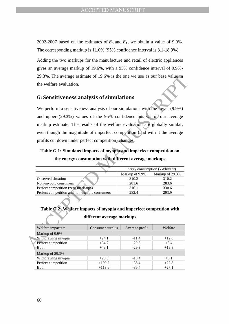
ACCEPTED MANUSCRIPT
ACCEPTED MANUSCRIP
T
60
2002-2007 based on the estimates of and , we obtain a value of 9.9%.
The corresponding markup is 11.0% (95% confidence interval is 3.1-18.9%).
Adding the two markups for the manufacture and retail of electric appliances
gives an average markup of 19.6%, with a 95% confidence interval of 9.9%-
29.3%. The average estimate of 19.6% is the one we use as our base value in
the welfare evaluation.
G: Sensitiveness analysis of simulations
We perform a sensitiveness analysis of our simulations with the lower (9.9%)
and upper (29.3%) values of the 95% confidence interval of our average
markup estimate. The results of the welfare evaluation are globally similar,
even though the magnitude of imperfect competition (and with it the average
profits cut down under perfect competition) changes.
Table G.1: Simulated impacts of myopia and imperfect competition on
the energy consumption with different average markups
Energy consumption (kWh/year)
Markup of 9.9% Markup of 29.3%
Observed situation 310.2 310.2
Non-myopic consumers 281.6 283.6
Perfect competition (zero mark-ups) 316.1 330.6
Perfect competition and non-myopic consumers 282.4 293.9
Table G.2: Welfare impacts of myopia and imperfect competition with
different average markups
Welfare impacts * Consumer surplus Average profit Welfare
Markup of 9.9%
Withdrawing myopia +24.1 -11.4 +12.8
Perfect competition +34.7 -29.3 +5.4
Both +49.1 -29.3 +19.8
Markup of 29.3%
Withdrawing myopia +26.5 -18.4 +8.1
Perfect competition +109.2 -86.4 +22.8
Both +113.6 -86.4 +27.1

ACCEPTED MANUSCRIPT
ACCEPTED MANUSCRIP
T
61
*: unit is 2005 pounds. Values are for an average sale. When myopia prevails, we have
subtracted unforeseen energy costs from the consumer surplus. The sales-weighted average
price of products included in the welfare evaluation is 296 pounds.
H: Modifications to the set of controls used in the supply
equation
The regression below increases the stringency of the controls used in the
supply equation. We first introduce fully interacted fixed effects: by-nest by-
brand by-year fixed effects. Results lose some precision but are unchanged
compared to our baseline specification.

ACCEPTED MANUSCRIPT
ACCEPTED MANUSCRIP
T
62
Table H.1: Fixed effects 2SLS Estimation results for the price equation
with fully interacted fixed effects
Dependent variable Log. price of product j
Markup, 0.0759*
(1.79)
Year x nest dummies x brand dummies Yes
Product fixed effects Yes
Weak identification test
Kleibergen-Paap rk Wald F statistic 12.13
Max. IV bias 10-15%
Observations 2,421
Notes. t-statistics are in brackets. Standard errors are robust to heteroskedasticity and
clustered on products. Results marked with *, ** and *** are statistically significant
at 10%, 5% and 1%, respectively.
Another possibility is to introduce nest-specific or brand-specific quadratic
trends. Likewise, results are quite similar in magnitude.

ACCEPTED MANUSCRIPT
ACCEPTED MANUSCRIP
T
63
Table H.2: Fixed effects 2SLS Estimation results for the price equation
with nest-specific quadratic interactions between height and time
Dependent variable Log. price of
product j
Log. price of
product j
Markup, 0.0438**
(2.40)
0.0818***
(2.60)
Year x nest dummies Yes Yes
Year x brand dummies Yes Yes
Nest-specific quadratic interactions
between height and time
Yes No
Brand-specific quadratic interactions
between height and time
No Yes
Product fixed effects Yes Yes
Weak identification test
Kleibergen-Paap rk Wald F statistic 29.95 14.07
Max. IV bias <10% 10-15%
Observations 2,421 2,421
Notes. t-statistics are in brackets. Standard errors are robust to heteroskedasticity and
clustered on products. Results marked with *, ** and *** are statistically significant
at 10%, 5% and 1%, respectively.