consumer demand system estimation and value … consumer demand system estimation and value added...

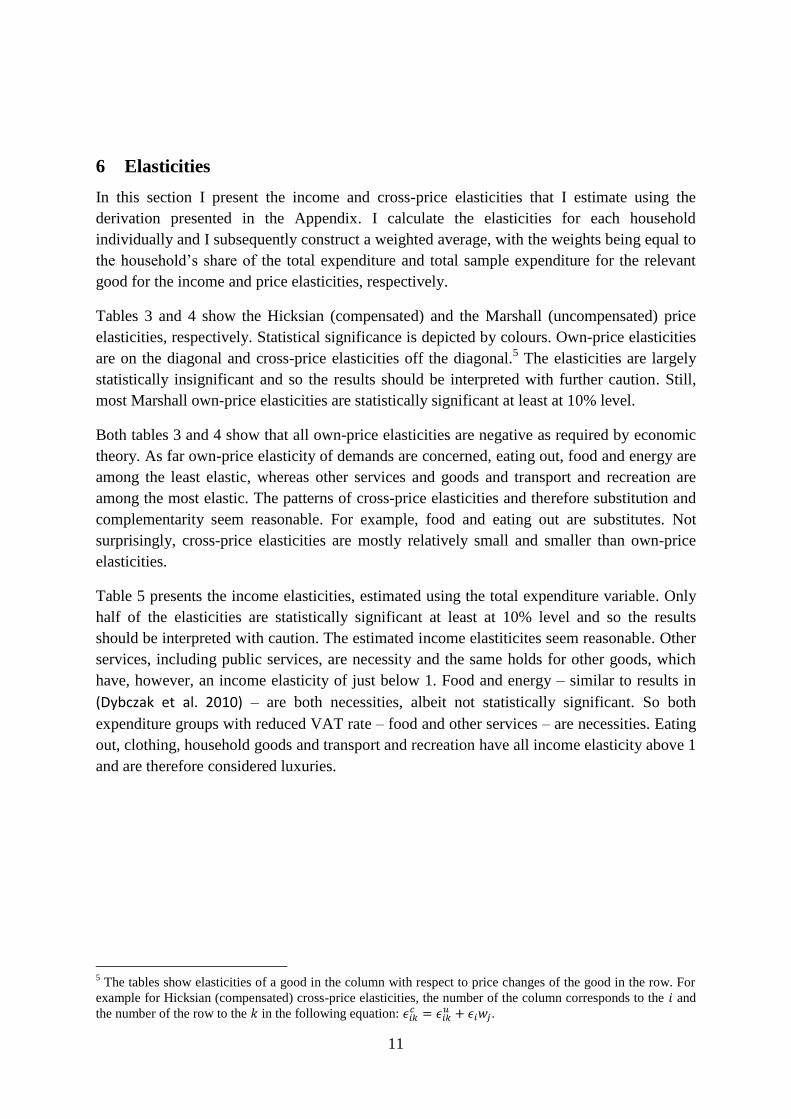
Consumer demand system estimation and value added tax reforms in the Czech Republic

IFS Working Paper W13/20

Petr Janský

1

Consumer Demand System Estimation and Value Added Tax Reforms in

the Czech Republic

Petr Janský

Institute of Economic Studies

Charles University in Prague

Abstract

Reforms of indirect taxes, such as the recent changes in rates of value added tax (VAT) in the

Czech Republic, change prices of products and services to which households can respond by

adjusting their expenditures. I estimate the behavioural response of consumers to price

changes in the Czech Republic applying a consumer demand model of the quadratic almost

ideal system (QUAIDS) form to the Czech Statistical Office data for the period from 2001 to

2011. I then derive the estimates of own- and cross-price and income elasticities and I use

these to estimate the impact of changes in VAT rates, which were proposed or implemented

between 2011 and 2013, on households and government revenues. I further find that this

method, which allows for behavioural response, yields lower estimates of changes in VAT

revenues than when I use the standard static simulation. These relatively small, but

statistically significant differences might partly explain the past cases, and might lead to

future cases, of the over-estimation of VAT revenues by the Ministry of Finance of the Czech

Republic.

Keywords

consumer behaviour; demand system; QUAIDS; value added tax; Czech Republic

JEL classification

D12; H20; H31

2

1 Introduction

Value added tax (VAT) is one of the most important taxes in the Czech Republic and the rest

of the developed world. The impact of VAT changes depends on microeconomic behaviour

of the consumers and my objective here is to shed more light on this and, more generally, on

household consumption and its taxation through VAT in the Czech Republic.

A rigorous analysis of impacts is desired especially in the Czech Republic since the reduced

and standard value added tax (VAT) rates have gone through important changes recently.

They were, respectively, 10% and 20% in 2011, 14% and 20% in 2012, and – after a last-

minute change from the previously approved unification of rates at 17.5% - a one percentage

point increase in both rates to 15% and 21% in 2013.

Existing impact evaluations of these VAT reforms have at best made use of first-order

approximations (e.g. (Dušek & Janský 2012a) and (Dušek & Janský 2012b)). These studies

used a standard method with no-behavioural-response static micro-simulation results and did

not properly account for the potential for consumers to substitute between goods as relative

prices change (Banks et al. 1996), which might cause over-estimation of the effects of tax

changes.

For a more rigorous analysis it is good to have a detailed knowledge of individual preferences

that are, of course, not readily available. So first, this paper derives second order

approximations which do not display systematic biases as shown in (Banks et al. 1996) and

require knowledge of the distribution of substitution elasticities, in contrast to first order

approximations. Specifically, I estimate Quadratic Almost Ideal Demand System (QUAIDS),

developed by (Banks et al. 1997) and applied for analysis of VAT reforms in Mexico by

(Abramovsky et al. 2012). In this demand system, similarly to the only previously QUAIDS

estimated for the Czech Republic by (Dybczak et al. 2010), demand depends not only on

prices and incomes, but also other household characteristics such as size of the household or

the employment status or age of the household head.

This almost ideal demand system allows me to take into account the consumers’ substitution

responses when relative prices change due to VAT reforms and is the first one in the Czech

Republic built specifically for the analysis of tax policy. The model uses household

expenditure and demographic data from the Household Budget Survey (HBS) and price data

from the Consumer Price Index (CPI). To the best of my knowledge, this demand system is

the first one in the Czech Republic built using only the consumer price information from CPI

rather than HBS. The exclusive use of official figures on prices in CPI instead of unit values

derived from expenditures and quantities recorded in HBS lowers the risk that observed price

variation may instead reflect variations in quality.

I chose categories of expenditure so that they reflect not only functional groupings (e.g. food,

clothes) but also reflect goods and services subject to different rates of VAT, i.e. in a similar

3

way to (Abramovsky et al. 2012). Estimated price and income elasticities appear plausible in

magnitude and sign. For instance, food is found to be a necessity while eating out is found to

be a luxury. Strong luxuries include transport and recreation and household goods. This

categorization, in combination with a simple VAT simulator, allows me to estimate how

consumers respond to changes in VAT rates and the implications for consumers’ spending

patterns and government’s tax revenues. I demonstrate this on the simulation of recent VAT

reforms. I find that allowing for behavioural response makes difference to estimates of the tax

revenues that are lower in comparison to the first order approximation holding behaviour

fixed, specifically the standard static micro-simulation model allowing for no behavioural

response and holding the quantity of purchases fixed (nominal expenditures rise or fall in line

with the rise of fall in VAT rates).

The layout of the paper is as follows. Section 2 provides a brief literature review. In section 3,

I discuss the theoretical consumer demand model and in the Appendix I show the derivation

of the formulae for the estimation of elasticities. Section 4 describes the data. In section 5, I

explain the estimation of the model. Section 6 discusses the results in the form of the

estimated elasticities. Section 7 outlines the application of the model’s results to the

evaluation of changes in VAT rates. Section 8 concludes.

4

2 Literature review

The literature on consumer demand and VAT is quite voluminous and I will therefore focus

only on three areas. First, I briefly introduce the most important contributions to demand

system estimation. Second, I discuss the existing articles estimating demand systems for the

Czech Republic. Third, I provide an overview of the literature on impacts of VAT in the

Czech Republic.

First, (Stone 1954) was the first to estimate a demand system based on consumer preferences

theory, specifically the linear expenditure systems developed by (Klein & Rubin 1947). A

number of improvements have been developed and proposed over the decades; nowadays

there are two main demand systems that are being estimated. The first is the Almost Ideal

Demand System (AIDS) developed by (Deaton & Muellbauer 1980), the second is the

Quadratic Almost Ideal Demand System (QUAIDS), developed by (Banks et al. 1997).

QUAIDS is basically AIDS that allows Engel curves to be quadratic. Furthermore, (Poi 2002)

and (Poi 2008) are useful introductions to estimating QUAIDS using the STATA software as

I do. Recent applications of QUAIDS model similar to this paper are (Crawford et al. 2010),

who discuss the implications of VAT for labour market participation on UK data, and

(Abramovsky et al. 2012), who evaluate Mexican VAT reform.

Second, I discuss the existing demand systems for the Czech Republic. The demand systems

have been estimated for the Czech Republic recently by two teams of researchers. Using the

AIDS in modification by (Edgerton 1996), (Janda et al. 2010) estimate elasticities with focus

on alcohol beverages and find, for example, a very low own-price elasticity of demand for

beer. (Dybczak et al. 2010) are the first to estimate the QUAIDS for the Czech Republic and

divide the expenditure into eight categories - food, clothing, energy, house, health, transport,

education and other - that do not align with VAT rates as is the case in this paper. They

estimate own- and cross-price and income elasticities and use them to analyse the impact of

changes in regulated prices on consumer demand. In addition, a number of studies such as

(Dubovicka et al. 1997) or (Janda et al. 2000) have focused on estimating Czech food demand

elasticities using flexible function forms, to which also both AIDS and QUAIDS belong.

Furthermore, (Crawford et al. 2004) develop a new method for estimation of price reactions

and apply it on the Czech data.

Third, I provide a short overview of VAT in the Czech Republic and related literature. The

Czech Republic introduced VAT in 1993 and it applies to most of household expenditures in

the form of its two rates. From 2013, the increased both its reduced and standard rates by one

percentage point to 15 % and 21 %, respectively. VAT and its changes in the Czech Republic

have been studied by (Schneider 2004), who analysed tax burden of households and found

VAT to be relatively regressive, and more recently by (Klazar et al. 2007), who focused on

the impact of EU-accession related harmonisation of VAT rates. (Klazar & Slintáková 2010)

studied the VAT in the Czech Republic and its impact on households and found VAT to be

5

regressive when annual income is analysed while their lifetime income analysis indicated that

VAT is progressive. (Dušek & Janský 2012a) and (Dušek & Janský 2012b) used a simple

micro-simulator – without using a demand system and accounting for behavioural response to

VAT changes as in this paper – to provide first independent estimates of the impact of the

recently proposed VAT rates changes in the Czech Republic on the living standards of

households and tax revenues. One objective of this paper is to compare the results of analysis

of these VAT reforms according to whether behavioural change is taken into account or not.

6

3 Theory

I estimate the demand system of the Quadratic Almost Ideal Demand System (QUAIDS)

form developed in (Banks et al. 1997) and I further use it for indirect tax policy analysis, as

proposed by (Banks et al. 1996) and applied in, for example, (Crawford et al. 2010) or

(Abramovsky et al. 2012). The QUAIDS model is a generalization of Almost Ideal Demand

System (AIDS) model that allows for quadratic Engel curves. The QUAIDS can therefore

allow a good to be a luxury at one level of income and a necessity at another, a property that

(Banks et al. 1997) find to be of empirical relevance for the UK and (Dybczak et al. 2010) do

the same for the Czech Republic.1 (Banks et al. 1997) also showed that it is sufficient for the

nonlinear term to be a quadratic in log income.

I introduce the QUAIDS model, basically as presented in (Banks et al. 1997), in the

Appendix. The model does not allow for positive or negative externalities from expenditure

on certain goods, for instance fuel, alcohol and tobacco. The assumption of no externalities

can be easily neither altered nor tested and is a limitation on the usefulness of QUAIDS, for

example, when looking at the welfare effects of excise duties on goods with negative

externalities.

1 Even earlier studies than (Banks et al. 1997) identified the importance of further terms in income for some, but

not all, expenditure share equations, see for example (Atkinson et al. 1990) or (Blundell et al. 1993) and (Banks

et al. 1997) for further discussion and references. This has been documented for the Czech Republic for the first

time by (Dybczak et al. 2010).

7

4 Data

To estimate QUAIDS in the Czech Republic I employ the best available data: two datasets

from the Czech Statistical Office (CSO). The Household Budget Survey (HBS) is a

representative sample of around 3000 Czech households. For each of them, HBS contains

information on how much they spend on various goods and services (around 250 expenditure

items), who they are (around 60 demographic variables) and how they earn their income

(around 30 income items).2 The HBS data is basically a pooled repeated cross-section data

set, and has been applied for estimation of the demand systems by both (Janda et al. 2010)

and (Dybczak et al. 2010). I employ data for the period between 2001 and 2011 and therefore

I have around 33000 households in total.

I use the CSO price data gathered for the purpose of the Consumer Price Index (CPI) that is

classified into around 150 categories according to the classification of individual

consumption by purpose (COICOP).3 The price information is available for the Czech

Republic as a whole and also separately for the capital city of Prague.

In the following part, I discuss two reasons why I opt to use the CPI as the only source of

prices. This is in contrast to both (Janda et al. 2010) and (Dybczak et al. 2010), who divided

the expenditures by the amount of purchased goods and services. This way, they obtained

unit values, which they used as prices. Not only can this method be in some cases inaccurate,

but also the HBS data for amounts of purchased goods and services is incomplete.

First, the HBS includes information on amounts of purchased goods and services only for a

limited number of expenditure items. Unit values can be thus constructed only for those

goods for which quantity information is available in the HBS. Therefore I would need to limit

my analysis to a small subset of overall expenditures, which was basically done by (Janda et

2 The CSO gathered the data in a way that only those for the period 2006-2011 can be considered fully

representative, but as some preliminary robustness checks did not find significant differences between the two

periods and since (Dybczak et al. 2010) showed the same, I conclude that there is no significant risk in using the

data for the longer period. Furthermore I use the representativeness weights provided by the CSO so that the

data reflect the overall Czech population. Still there are some further concerns for the real representativeness of

this data, especially with its earlier editions. Although treatments of the potential problems of this nature are

generally beyond the scope of this analysis, let me briefly review them. Earlier, the CSO was criticized for

failing to provide the full dataset of HBS to European Union representatives (Eurostat 2009). Furthermore, as

(Crawford & Z. Smith 2002) discuss, systematic over- or under-reporting of expenditures can occur due to

forgetfulness (e.g., consumption outside the home), active concealment (e.g., receipt from a beauty studio), and

guilt (e.g., cigarettes) . Another problem mentioned by (Crawford & Z. Smith 2002) that may occur in the Czech

HBS is the following: as expenditures are recorded monthly, large and infrequent purchases may be

underestimated. And this is also one of the reasons why I exclude housing from the expenditure data, both

purchase and rent (the corresponding HBS codes in the 2011 data are 4010, 4080, 5440, 5550). Furthermore the

relatively high and infrequent housing expenditures would distort the model. This is a common approach in the

existing literature, for example (Banks et al. 1997). 3 Some prices are regulated in the Czech Republic, either nationally (health care fees) locally (waste disposal

service charge) and would therefore arguably require a special treatment, which I however do not provide here

because of the complexity and because the share of regulated prices is very low.

8

al. 2010), or fill in the HBS unit values whenever these are not available by the CPI prices,

which was done by (Dybczak et al. 2010). In contrast to (Janda et al. 2010), I prefer to analyse

an as high share of overall household consumption as possible, which is made possible by

applying the CPI data. In contrast to (Dybczak et al. 2010), I prefer the consistency of using

only one complete source for the information on prices, the CPI. Second, the differences in

unit values can be caused by product quality differences rather than price differences that I

aim to study. With the unit values it is almost impossible to distinguish between the influence

of changes in prices and quality since risk observed price variation may instead reflect

variations in quality. By using the CPI data, I limit the extent of this problem.

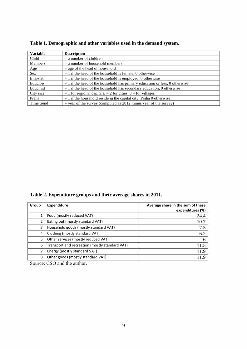
In the expenditure share equations estimated in QUAIDS I further include a time trend and a

number of demographic variables to control for preference variation that may be correlated

with total expenditure or prices in a way that is consistent with the model. Table 1 provides

the list of these variables.

I classify the HBS expenditure data according to the VAT rates, reduced and standard,

presented in the appendices to the law on VAT as of January 2013. When HBS classification

is not detailed enough to allow the accurate division according to the VAT rate or when some

expenditures are exempted from VAT, I assign the VAT rate according to the one prevailing

for that group. I merge the HBS and the CPI data using the HBS codes and COICOP codes

and although these two classifications do not always match well, no significant compromises

had to be made during the matching process.

In order to estimate QUAIDS, I divided the detailed expenditure items into eight groups. I

have followed three principles while grouping the expenditure items and in this I differ from

the previously estimated demand systems for the Czech Republic. First, the division should

correspond to natural categories as people think about them, as is done for example by

(Dybczak et al. 2010). Second, the expenditure groups should be of a similar size. Third and

most important for my analysis, expenditure groups should be divided according to VAT

rates as much as possible. A number of compromises had to be made when following these

three principles and I have given most weight to the third one. I calculate the price indices of

aggregated commodities as weighted arithmetic averages of the price indices of the individual

goods and services making up the aggregated commodity. Table 2 provides the names and

shares in total expenditures of the eight expenditure groups for the year of 2011. There is a

more detailed description in Table A1 and basic summary statistics in Table A2 in the

Appendix. I use this categorisation of expenditures into groups in the following analysis.

9

Table 1. Demographic and other variables used in the demand system.

Variable Description

Child = a number of children

Members = a number of household members

Age = age of the head of household

Sex = 1 if the head of the household is female, 0 otherwise

Empstat = 1 if the head of the household is employed, 0 otherwise

Educlow = 1 if the head of the household has primary education or less, 0 otherwise

Educmid = 1 if the head of the household has secondary education, 0 otherwise

City size = 1 for regional capitals, = 2 for cities, 3 = for villages

Praha = 1 if the household reside in the capital city, Praha 0 otherwise

Time trend = year of the survey (computed as 2012 minus year of the survey)

Table 2. Expenditure groups and their average shares in 2011.

Group Expenditure Average share in the sum of these expenditures (%)

1 Food (mostly reduced VAT) 24.4

2 Eating out (mostly standard VAT) 10.7

3 Household goods (mostly standard VAT) 7.5

4 Clothing (mostly standard VAT) 6.2

5 Other services (mostly reduced VAT) 16

6 Transport and recreation (mostly standard VAT) 11.5

7 Energy (mostly standard VAT) 11.9

8 Other goods (mostly standard VAT) 11.9

Source: CSO and the author.

10

5 Estimation

The estimation of QUAIDS follows two stages and is similar as in, for example,

(Abramovsky et al. 2012). At the first stage of the estimation, the values of and are

unknown to me and therefore I approximate as 1 and , using the Stone price

index named after (Stone 1954), as:

.

QUAIDS is linear in parameters conditional upon the price indices and, therefore, I can and

do employ a linear Seemingly Unrelated Regression (SUR) method to estimate the model.

Adding up is imposed by excluding the equation for the nth good from the estimated system

of equations; parameters for this equation are calculated using the parameters from the other

(n-1) equations and the adding up restrictions (the results are not by construction sensitive to

the choice of the nth good). Homogeneity (by expressing all prices relative to the price of the

other remaining goods) and symmetry are imposed using linear restrictions on parameters.

The parameters estimated at the first stage are then used to calculate values for and

. The model is then re-estimated using the same specification as the first stage except

that is replaced with and by

. The new parameter values are used to update

and , and the model is then re-estimated for a third time. This updating of price

indices and re-estimation is iterated 8 times, by which time the parameter values have

converged to 4 decimal places.

I instrument for expenditure using monetary income because it may be endogenous. I do so

using a control function approach as is common in the literature and as applied in (Banks et

al. 1997) or (Abramovsky et al. 2012).4 I calculate standard errors using bootstrapping with

1300 iterations with clustering at the household level.

Table A3 in the Appendix presents the parameter estimates for the QUAIDS. It is difficult to

interpret the parameters of QUAIDS directly and I will therefore discuss the elasticities as is

also common in the existing literature.

4 I regress the log of total expenditure (lnx) and the square of the log of total expenditure (lnx)

2 on the prices and

demographic variables included in the demand system and on the log of household monetary income and the

square of the log of household monetary income and include linear, square and cubic terms of the residuals from

these regressions in our demand system equations.

11

6 Elasticities

In this section I present the income and cross-price elasticities that I estimate using the

derivation presented in the Appendix. I calculate the elasticities for each household

individually and I subsequently construct a weighted average, with the weights being equal to

the household’s share of the total expenditure and total sample expenditure for the relevant

good for the income and price elasticities, respectively.

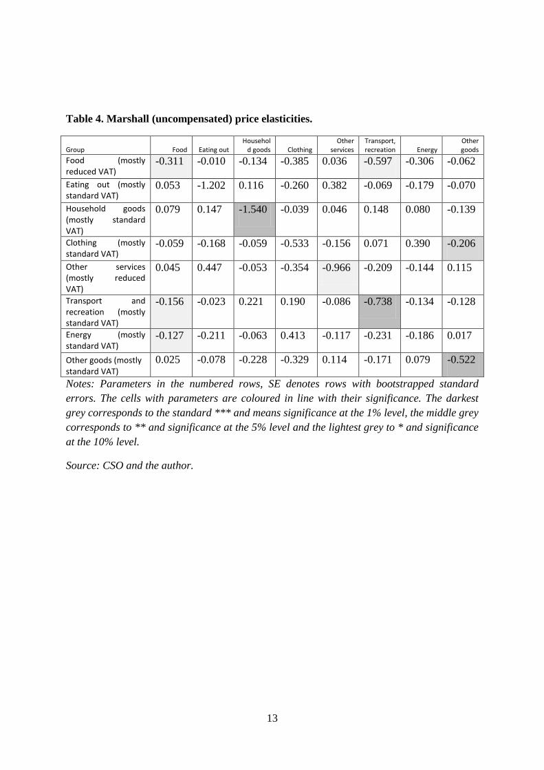
Tables 3 and 4 show the Hicksian (compensated) and the Marshall (uncompensated) price

elasticities, respectively. Statistical significance is depicted by colours. Own-price elasticities

are on the diagonal and cross-price elasticities off the diagonal.5 The elasticities are largely

statistically insignificant and so the results should be interpreted with further caution. Still,

most Marshall own-price elasticities are statistically significant at least at 10% level.

Both tables 3 and 4 show that all own-price elasticities are negative as required by economic

theory. As far own-price elasticity of demands are concerned, eating out, food and energy are

among the least elastic, whereas other services and goods and transport and recreation are

among the most elastic. The patterns of cross-price elasticities and therefore substitution and

complementarity seem reasonable. For example, food and eating out are substitutes. Not

surprisingly, cross-price elasticities are mostly relatively small and smaller than own-price

elasticities.

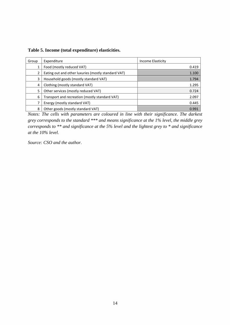
Table 5 presents the income elasticities, estimated using the total expenditure variable. Only

half of the elasticities are statistically significant at least at 10% level and so the results

should be interpreted with caution. The estimated income elastiticites seem reasonable. Other

services, including public services, are necessity and the same holds for other goods, which

have, however, an income elasticity of just below 1. Food and energy – similar to results in

(Dybczak et al. 2010) – are both necessities, albeit not statistically significant. So both

expenditure groups with reduced VAT rate – food and other services – are necessities. Eating

out, clothing, household goods and transport and recreation have all income elasticity above 1

and are therefore considered luxuries.

5 The tables show elasticities of a good in the column with respect to price changes of the good in the row. For

example for Hicksian (compensated) cross-price elasticities, the number of the column corresponds to the and

the number of the row to the in the following equation:

.

12

Table 3. Hicksian (compensated) price elasticities.

Group Food Eating out Househol

d goods Clothing Other

services Transport, recreation Energy

Other goods

Food (mostly reduced VAT)

-0.194 0.243 0.257 -0.092 0.214 -0.214 -0.206 0.170

Eating out (mostly standard VAT)

0.100 -1.081 0.304 -0.121 0.464 0.120 -0.139 0.038

Household goods (mostly standard VAT)

0.117 0.253 -1.366 0.088 0.115 0.331 0.113 -0.045

Clothing (mostly standard VAT)

-0.026 -0.082 0.078 -0.431 -0.098 0.211 0.416 -0.131

Other services (mostly reduced VAT)

0.111 0.603 0.187 -0.175 -0.851 0.029 -0.090 0.256

Transport and recreation (mostly standard VAT)

-0.101 0.135 0.492 0.397 0.013 -0.414 -0.079 0.013

Energy (mostly standard VAT)

-0.080 -0.112 0.091 0.526 -0.050 -0.081 -0.139 0.112

Other goods (mostly standard VAT)

0.073 0.040 -0.042 -0.192 0.195 0.018 0.123 -0.413

Notes: Parameters in the numbered rows, SE denotes rows with bootstrapped standard

errors. The cells with parameters are coloured in line with their significance. The darkest

grey corresponds to the standard *** and means significance at the 1% level, the middle grey

corresponds to ** and significance at the 5% level and the lightest grey to * and significance

at the 10% level.


13

Table 4. Marshall (uncompensated) price elasticities.

Group Food Eating out Househol

d goods Clothing Other

services Transport, recreation Energy

Other goods

Food (mostly reduced VAT)

-0.311 -0.010 -0.134 -0.385 0.036 -0.597 -0.306 -0.062

Eating out (mostly standard VAT)

0.053 -1.202 0.116 -0.260 0.382 -0.069 -0.179 -0.070

Household goods (mostly standard VAT)

0.079 0.147 -1.540 -0.039 0.046 0.148 0.080 -0.139

Clothing (mostly standard VAT)

-0.059 -0.168 -0.059 -0.533 -0.156 0.071 0.390 -0.206

Other services (mostly reduced VAT)

0.045 0.447 -0.053 -0.354 -0.966 -0.209 -0.144 0.115

Transport and recreation (mostly standard VAT)

-0.156 -0.023 0.221 0.190 -0.086 -0.738 -0.134 -0.128

Energy (mostly standard VAT)

-0.127 -0.211 -0.063 0.413 -0.117 -0.231 -0.186 0.017

Other goods (mostly standard VAT)

0.025 -0.078 -0.228 -0.329 0.114 -0.171 0.079 -0.522

Notes: Parameters in the numbered rows, SE denotes rows with bootstrapped standard

errors. The cells with parameters are coloured in line with their significance. The darkest



at the 10% level.


14

Table 5. Income (total expenditure) elasticities.

Group Expenditure Income Elasticity

1 Food (mostly reduced VAT) 0.419

2 Eating out and other luxuries (mostly standard VAT) 1.100

3 Household goods (mostly standard VAT) 1.794

4 Clothing (mostly standard VAT) 1.295

5 Other services (mostly reduced VAT) 0.724

6 Transport and recreation (mostly standard VAT) 2.097

7 Energy (mostly standard VAT) 0.445

8 Other goods (mostly standard VAT) 0.991

Notes: The cells with parameters are coloured in line with their significance. The darkest



at the 10% level.


15

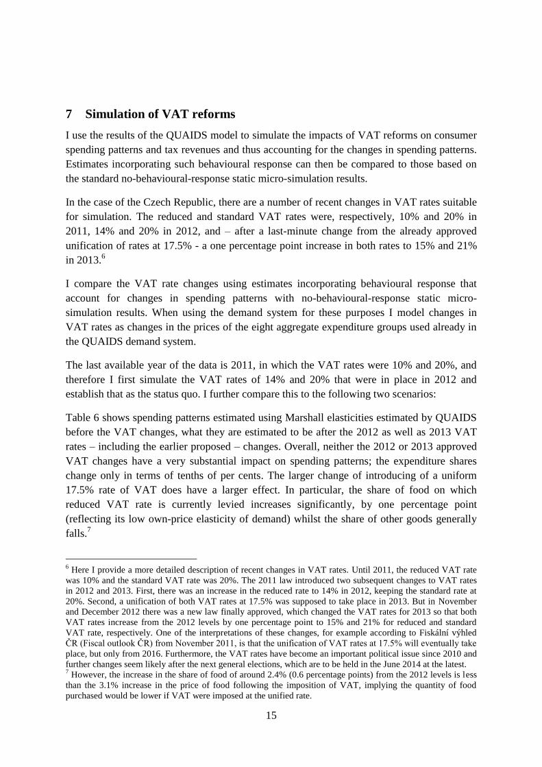
7 Simulation of VAT reforms

I use the results of the QUAIDS model to simulate the impacts of VAT reforms on consumer

spending patterns and tax revenues and thus accounting for the changes in spending patterns.

Estimates incorporating such behavioural response can then be compared to those based on

the standard no-behavioural-response static micro-simulation results.

In the case of the Czech Republic, there are a number of recent changes in VAT rates suitable

for simulation. The reduced and standard VAT rates were, respectively, 10% and 20% in

2011, 14% and 20% in 2012, and – after a last-minute change from the already approved

unification of rates at 17.5% - a one percentage point increase in both rates to 15% and 21%

in 2013.6

I compare the VAT rate changes using estimates incorporating behavioural response that

account for changes in spending patterns with no-behavioural-response static micro-

simulation results. When using the demand system for these purposes I model changes in

VAT rates as changes in the prices of the eight aggregate expenditure groups used already in

the QUAIDS demand system.

The last available year of the data is 2011, in which the VAT rates were 10% and 20%, and

therefore I first simulate the VAT rates of 14% and 20% that were in place in 2012 and

establish that as the status quo. I further compare this to the following two scenarios:

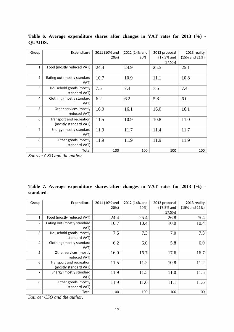
Table 6 shows spending patterns estimated using Marshall elasticities estimated by QUAIDS

before the VAT changes, what they are estimated to be after the 2012 as well as 2013 VAT

rates – including the earlier proposed – changes. Overall, neither the 2012 or 2013 approved

VAT changes have a very substantial impact on spending patterns; the expenditure shares

change only in terms of tenths of per cents. The larger change of introducing of a uniform

17.5% rate of VAT does have a larger effect. In particular, the share of food on which

reduced VAT rate is currently levied increases significantly, by one percentage point

(reflecting its low own-price elasticity of demand) whilst the share of other goods generally

falls.7

6 Here I provide a more detailed description of recent changes in VAT rates. Until 2011, the reduced VAT rate

was 10% and the standard VAT rate was 20%. The 2011 law introduced two subsequent changes to VAT rates

in 2012 and 2013. First, there was an increase in the reduced rate to 14% in 2012, keeping the standard rate at

20%. Second, a unification of both VAT rates at 17.5% was supposed to take place in 2013. But in November

and December 2012 there was a new law finally approved, which changed the VAT rates for 2013 so that both

VAT rates increase from the 2012 levels by one percentage point to 15% and 21% for reduced and standard

VAT rate, respectively. One of the interpretations of these changes, for example according to Fiskální výhled

ČR (Fiscal outlook ČR) from November 2011, is that the unification of VAT rates at 17.5% will eventually take

place, but only from 2016. Furthermore, the VAT rates have become an important political issue since 2010 and

further changes seem likely after the next general elections, which are to be held in the June 2014 at the latest. 7 However, the increase in the share of food of around 2.4% (0.6 percentage points) from the 2012 levels is less

than the 3.1% increase in the price of food following the imposition of VAT, implying the quantity of food

purchased would be lower if VAT were imposed at the unified rate.

16

Table 7 shows spending patterns in the same way as table 6, but using a standard method:

with no-behavioural-response static micro-simulation results and without the application of

the QUAIDS results. Specifically, the table shows the estimated expenditure shares from the

reforms using the static micro-simulation model allowing for no behavioural response and

holding the quantity of purchases fixed (nominal expenditures rise or fall in line with the rise

of fall in VAT rates).

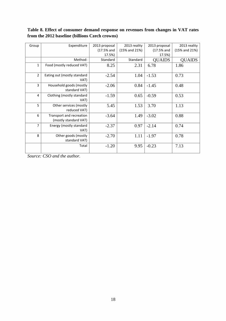
Table 8 shows revenue estimates for the VAT changes on the basis of our sample of Czech

households extrapolated for the whole population of the Czech Republic. Here I focus on the

analysis of the 2013 VAT changes. Therefore I consider and first simulate the 2012 VAT

rates of 14% and 20% as the baseline and compare it with both the approved reform of VAT

rates of 15% and 21% and the proposed reform of the unified VAT rate of 17.5%.

The first two columns of table 8 shows the estimated revenues from the reforms using the

standard static micro-simulation model allowing for no behavioural response and holding the

quantity of purchases fixed (standard). The third and fourth columns use the QUAIDS model

described above to allow spending patterns to change in response to the changes in prices.

The magnitude of difference between the two estimation methods used is in line with the

differences between results in tables 6 and 7: allowing for consumer spending patterns to

change has a relatively small, but significant impact on additional VAT revenues.

With the standard method the estimated impact on VAT revenues is, rounding these figures, -

1 billion CZK (Czech crowns) and 10 billion CZK for the 2013 proposal (unified VAT rate of

17.5%) and reality (15% and 21%), respectively. The corresponding estimates using

QUAIDS are around zero and 7 billion CZK, i.e. lower in total by around 1 billion CZK and,

as table 8 shows, also lower for individual expenditure groups than the standard estimates.

The estimated tax revenue after allowing for behaviour to adjust (in accordance with

QUAIDS preferences) is, as expected, lower than the estimate using the standard static

micro-simulation methodology that holds fixed the quantity of goods and services purchased.

These relatively small, but significant differences might partly explain the past cases, and

might lead to future cases of the over-estimation of VAT revenues by the Ministry of Finance

of the Czech Republic.

In the government budget report for 2013 (Ministry of Finance of the Czech Republic 2012)

(pages 12 and 13), the overall increase (mostly due to one percentage point increase in both

VAT rates and an expected increase in consumption) in VAT revenues is estimated at 1.2%

and at 9.8 billion CZK for central government and since around one third of VAT revenues

goes to the regional governments, this corresponds to around 14 billion CZK. Although my

estimates of around 10 and 8.5 billion CZK are limited in the sense that they cover only the

VAT revenues raised from household consumption and are therefore not directly comparable

with the Ministry’s numbers, my expert estimate is that the Ministry’s numbers are around

the upper bounds of - my - realistic estimates and that – depending on the growth of

household consumption in 2013 – their numbers might well be overestimated, partly by

failing to account for behavioural response.

17

Table 6. Average expenditure shares after changes in VAT rates for 2013 (%) -

QUAIDS.

Group Expenditure 2011 (10% and 20%)

2012 (14% and 20%)

2013 proposal (17.5% and

17.5%)

2013 reality (15% and 21%)

1 Food (mostly reduced VAT) 24.4 24.9 25.5 25.1

2 Eating out (mostly standard VAT)

10.7 10.9 11.1 10.8

3 Household goods (mostly standard VAT)

7.5 7.4 7.5 7.4

4 Clothing (mostly standard VAT)

6.2 6.2 5.8 6.0

5 Other services (mostly reduced VAT)

16.0 16.1 16.0 16.1

6 Transport and recreation (mostly standard VAT)

11.5 10.9 10.8 11.0

7 Energy (mostly standard VAT)

11.9 11.7 11.4 11.7

8 Other goods (mostly standard VAT)

11.9 11.9 11.9 11.9

Total 100 100 100 100


Table 7. Average expenditure shares after changes in VAT rates for 2013 (%) -

standard.

Group Expenditure 2011 (10% and 20%)

2012 (14% and 20%)


17.5%)

2013 reality (15% and 21%)

1 Food (mostly reduced VAT) 24.4 25.4 26.8 25.4 2 Eating out (mostly standard

VAT) 10.7 10.4 10.0 10.4


7.5 7.3 7.0 7.3


6.2 6.0 5.8 6.0


16.0 16.7 17.6 16.7


11.5 11.2 10.8 11.2


11.9 11.5 11.0 11.5


11.9 11.6 11.1 11.6

Total 100 100 100 100


18

Table 8. Effect of consumer demand response on revenues from changes in VAT rates

from the 2012 baseline (billions Czech crowns)

Group Expenditure 2013 proposal (17.5% and

17.5%)

2013 reality (15% and 21%)


17.5%)

2013 reality (15% and 21%)

Method: Standard Standard QUAIDS QUAIDS 1 Food (mostly reduced VAT) 8.25 2.31 6.78 1.86

2 Eating out (mostly standard VAT)

-2.54 1.04 -1.53 0.73


-2.06 0.84 -1.45 0.48


-1.59 0.65 -0.59 0.53


5.45 1.53 3.70 1.13


-3.64 1.49 -3.02 0.88


-2.37 0.97 -2.14 0.74


-2.70 1.11 -1.97 0.78

Total -1.20 9.95 -0.23 7.13


19

8 Conclusion

In this paper I have employed detailed data of Czech Statistical Office to estimate a consumer

demand model of the quadratic almost ideal system (QUAIDS), derived the own- and cross-

price and income elasticities and simulated the impacts of recent VAT reforms for the Czech

Republic. Accounting for behavioural response yielded significantly different estimates of

impacts of the reforms on the government revenues. The estimated tax revenue after allowing

for behaviour to adjust (in accordance with QUAIDS preferences) is modestly, but

significantly lower than the estimate using the standard static micro-simulation methodology

that holds fixed the quantity of goods and services purchased. This contributes to the existing

simulation of VAT reforms in the Czech Republic (Dušek & Janský 2012a) and (Dušek &

Janský 2012b) and in other countries, including most Mexico (Abramovsky et al. 2012).

There are a number of interesting areas for further research. For example, when data for 2012

and 2013 are available, it should be interesting and enriching to look at the actual behaviour

of consumers and, also, to compare it with the estimates of the models. Furthermore, there are

a number of ways in which to estimate QUAIDS and similar models and it would be

desirable to explore these for the Czech Republic. These options include the expenditures

included and excluded in the demand system (such as exclusion of housing in most demand

system including this estimation), the number of expenditure groups and division of goods

among these groups, whether and how I deal with outlier data, whether and what taste shifters

and demographic characteristics to include, time period and frequency, unit value prices or

other, external prices, ways of computing elasticities (weighted average in this estimation or

for a representative or an average household), a homogeneous or representative sample of the

population.

20

9 References

Abramovsky, L., Attanasio, O. & Phillips, D., 2012. Demand responses to changes in

consumer prices in Mexico: lessons for policy and an application to the 2010 Mexican

tax reforms. IFS mimeo.

Atkinson, A.B., Gomulka, J. & Stern, N.H., 1990. Spending on alcohol: evidence from the

family expenditure survey 1970-1983. The Economic Journal, 100(402), pp.808–827.

Banks, J., Blundell, R. & Lewbel, A., 1997. Quadratic Engel curves and consumer demand.

Review of Economics and Statistics, 79(4), pp.527–539.

Banks, J., Blundell, R. & Lewbel, A., 1996. Tax reform and welfare measurement: do we

need demand system estimation? The Economic Journal, 106(438), pp.1227–1241.

Blundell, R., Pashardes, P. & Weber, G., 1993. What do we learn about consumer demand

patterns from micro data? The American Economic Review, pp.570–597.

Crawford, I., Keen, M. & Smith, S., 2010. Value added tax and excises. Dimensions of Tax

Design: The Mirrlees Review, pp.275–362.

Crawford, I., Laisney, F. & Preston, I., 2004. Estimation of Household Demand Systems with

Theoretically Compatible Engel Curves and Unit Value Specifications. Journal of

Econometrics.

Crawford, I. & Smith, Z., 2002. Distributional aspects of inflation. Available at:

http://www.ifs.org.uk/comms/comm90.pdf [Accessed October 15, 2012].

Deaton, A. & Muellbauer, J., 1980. An almost ideal demand system. The American Economic

Review, 70(3), pp.312–326.

Dubovicka, S., Volosin, J. & Janda, K., 1997. Czech import demand for agricultural and food

products from OECD countries. Zemedelska Ekonomika-UZPI (Czech Republic).

Dušek, L. & Janský, P., 2012a. Changes in value added tax: how much do they affect

households? (Změny daně z přidané hodnoty: Kolik přidají nebo uberou

domácnostem?). Politická ekonomie, (3).

Dušek, L. & Janský, P., 2012b. Tax reform proposals: how much do they bring to the public

sector budgets? (Návrhy daňových změn: kolik přidají veřejným rozpočtům?).

Ekonomická revue - Central European Review of Economic Issues, 15(1), pp.51–62.

Dybczak, K., Tóth, P. & Voňka, D., 2010. Effects of Price Shocks to Consumer Demand.

Estimating the QUAIDS Demand System on Czech Household Budget Survey Data.

Working Papers.

Edgerton, D.L., 1996. The econometrics of demand systems: with applications to food

demand in the Nordic countries, Springer.

21

Eurostat, 2009. Improving data comparability for the next HBS round (2010). Available at:

http://epp.eurostat.ec.europa.eu/cache/ITY_SDDS/Annexes/hbs_esms_an5.pdf.

Janda, K., McCluskey, J.J. & Rausser, G.C., 2000. Food import demand in the Czech

Republic. Journal of Agricultural Economics, 51(1), pp.22–44.

Janda, K., Mikolášek, J. & Netuka, M., 2010. Complete almost ideal demand system

approach to the Czech alcohol demand. Agricultural Economics-UZEI, 56.

Klazar, S. et al., 2007. Dopad harmonizace sazeb DPH v ČR. Acta Oeconomica Pragensia,

15(1), pp.45–55.

Klazar, S. & Slintáková, B., 2010. Impact of Harmonisation on Distribution of VAT in the

Czech Republic. Prague Economic Papers, 2010(2), pp.133–149.

Klein, L.R. & Rubin, H., 1947. A constant-utility index of the cost of living. The Review of

Economic Studies, 15(2), pp.84–87.

Ministry of Finance of the Czech Republic, 2012. Zpráva k návrhu zákona o státním rozpočtu

ČR na rok 2013. Available at:

https://www.google.cz/url?sa=t&rct=j&q=&esrc=s&source=web&cd=3&cad=rja&ve

d=0CEUQFjAC&url=http%3A%2F%2Fwww.psp.cz%2Fsqw%2Ftext%2Forig2.sqw

%3Fidd%3D123469&ei=_Iv5ULO-

EdGSswaLgYHoDA&usg=AFQjCNGQ6QD3enCFlddXKKN6NR6HrT6-

zg&sig2=XfnB7Rtx1I-Ff1qn1poppw&bvm=bv.41248874,d.Yms.

Poi, B.P., 2008. Demand-system estimation: Update. Stata Journal, 8(4), pp.554–556.

Poi, B.P., 2002. From the help desk: Demand system estimation. Stata Journal, 2(4), pp.403–

410.

Schneider, O., 2004. Who Pays Taxes and Who Gets Benefits in the Czech Republic. Prague

Economic Papers No. 2005/3.

Stone, R., 1954. Linear expenditure systems and demand analysis: an application to the

pattern of British demand. The Economic Journal, 64(255), pp.511–527.

22

10 Appendix

10.1 QUAIDS model

This section introduces the QUAIDS model, basically as presented in (Banks et al. 1997).

QUAIDS is based on the following indirect utility8:

Where x is total expenditure, p stands for prices, , , and are defined as:

where i=1,..., n denotes a good, is the translog price aggregator function, and is

defined as the simple Cobb-Douglas price aggregator.

Applying Roy’s identity to the equation for , I have the following equations for ,

the share of expenditure on good i in total expenditure for each household:

These budget shares are quadratic in

and, as (Banks et al. 1997) demonstrate,

quadratic in itself. For the resulting demands to be consistent with utility maximisation,

the demand system must satisfy four key properties: adding-up; homogeneity; symmetry; and

negativity (negative semi-definiteness). Only negativity cannot be imposed but the estimated

Slutsky matrix can be tested to see if it satisfies this criterion. The first three properties can be

imposed using linear restrictions on the parameters of the model:

(adding up)

8 The same indirect utility function defines the AIDS model, but with the term set to zero.

23

(homogeneity)

(symmetry)

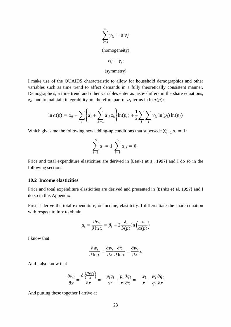
I make use of the QUAIDS characteristic to allow for household demographics and other

variables such as time trend to affect demands in a fully theoretically consistent manner.

Demographics, a time trend and other variables enter as taste-shifters in the share equations,

, and to maintain integrability are therefore part of terms in :

Which gives me the following new adding-up conditions that supersede :

Price and total expenditure elasticities are derived in (Banks et al. 1997) and I do so in the

following sections.

10.2 Income elasticities

Price and total expenditure elasticities are derived and presented in (Banks et al. 1997) and I

do so in this Appendix.

First, I derive the total expenditure, or income, elastitcity. I differentiate the share equation

with respect to to obtain

I know that

And I also know that

And putting these together I arrive at

24

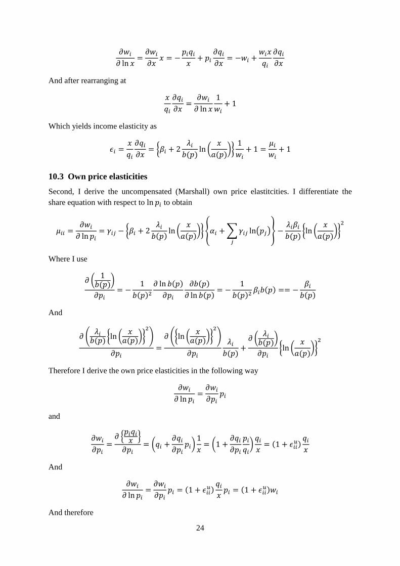
And after rearranging at

Which yields income elasticity as

10.3 Own price elasticities

Second, I derive the uncompensated (Marshall) own price elastitcities. I differentiate the

share equation with respect to to obtain

Where I use

And

Therefore I derive the own price elasticities in the following way

and

And

And therefore

25

I arrive at

which is the uncompensated own price elasticity.

I use the Slutsky equation,

, to calculate the set of compensated (Hicksian)

elasticities, .

10.4 Cross price elasticities

Third, I derive the uncompensated (Marshall) cross price elastitcities. I differentiate the share

equation with respect to to obtain

Where I use

and

And

And therefore

I arrive at

26

which is the uncompensated cross price elasticity.

The uncompensated price elasticity, both cross and own, could be written as

where is the Kronecker delta (a value of 1 if the variables are equal, and 0 otherwise).

I use the Slutsky equation,

, to calculate the set of compensated (Hicksian)

elasticities, .

I also use to assess the symmetry and negativity conditions by examining the matrix with

elements , which should be symmetric and negative semidefinite in the usual way.

27

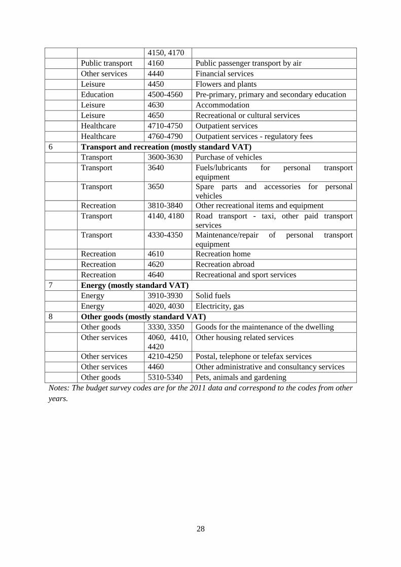
10.5 Definition of expenditure groups

Table A1. Definition of expenditure groups.

Group Expenditure HBS code Expenditure items

1 Food (mostly reduced VAT)

Food 2010-2820,

2860, 2870,

2890, 2910

Meat, oils and fats, milk, cheese, eggs, bread

and cereals, vegetables, fruit, sugar, chocolate,

confectionery, coffee, tea and cocoa, mineral

waters, soft drinks, school and kindergarten

cafeteria

2 Eating out and other luxuries (mostly standard VAT)

Eating out 2880, 2900,

2920-2970

Cafeterias and eating out, drinks out

Alcoholic

beverages

2830-2850 Alcoholic beverages

Tobacco 3900 Tobacco

Cosmetics 3320, 3340,

4430

Cosmetics, hairdressing


Household goods 3400-3490 Furniture and furnishings

Household goods 3510-3570 Household appliances

Household goods 3660 Children prams

Household goods 3700 Mobile phones

Household goods 3710-3760 Audio-visual, photographic, information

technology equipment

Household goods 3770-3790 Communication appliances, toys and other

goods

Household goods 3850 Stationery

Household goods 4360, 4370 Maintenance or repair of household appliances

Household goods 4380 Repair of audio-visual, photographic,

information technology equipment


Clothing 3010-3100 Clothing

Clothing 3210-3270 Footwear

Clothing 3310 Washing goods for clothes

Clothing 4310 Repair or hire of clothing

Clothing 4320 Repair or hire of footwear

5 Public and other services (mostly reduced VAT)

Healthcare 3300, 3370,

3380

Medicaments

Healthcare 3360, 3390 Medical products and appliances

Leisure 3860-3890 Newspapers and books

Other services 4040 Heat energy and hot water supply

Other services 4050 Cold water

Other services 4070 Trash collection service

Public transport 4110-4130, Public passenger transport by railway, road

28

4150, 4170

Public transport 4160 Public passenger transport by air

Other services 4440 Financial services

Leisure 4450 Flowers and plants

Education 4500-4560 Pre-primary, primary and secondary education

Leisure 4630 Accommodation

Leisure 4650 Recreational or cultural services

Healthcare 4710-4750 Outpatient services

Healthcare 4760-4790 Outpatient services - regulatory fees


Transport 3600-3630 Purchase of vehicles

Transport 3640 Fuels/lubricants for personal transport

equipment

Transport 3650 Spare parts and accessories for personal

vehicles

Recreation 3810-3840 Other recreational items and equipment

Transport 4140, 4180 Road transport - taxi, other paid transport

services

Transport 4330-4350 Maintenance/repair of personal transport

equipment

Recreation 4610 Recreation home

Recreation 4620 Recreation abroad

Recreation 4640 Recreational and sport services


Energy 3910-3930 Solid fuels

Energy 4020, 4030 Electricity, gas


Other goods 3330, 3350 Goods for the maintenance of the dwelling

Other services 4060, 4410,

4420

Other housing related services

Other services 4210-4250 Postal, telephone or telefax services

Other services 4460 Other administrative and consultancy services

Other goods 5310-5340 Pets, animals and gardening

Notes: The budget survey codes are for the 2011 data and correspond to the codes from other

years.

29

10.6 Summary statistics

Table A2. Summary statistics.

Variable Mean Standard

deviation

Minimum Maximum

Share of group 1 0.250528 0.083039 0.027277 0.772953

Share of group 2 0.10895 0.058785 0 0.634563

Share of group 3 0.086515 0.072745 0 0.766646

Share of group 4 0.074685 0.040686 0 0.396075

Share of group 5 0.151303 0.080748 0.000157 0.817917

Share of group 6 0.116551 0.111254 0 0.926354

Share of group 7 0.101474 0.074569 0 0.644764

Share of group 8 0.109995 0.058952 0 0.673282

Price of group 1 105.664 8.782365 95.76093 118.803

Price of group 2 104.7033 10.38965 91.95399 122.6353

Price of group 3 101.4283 12.96666 86.09968 127.8821

Price of group 4 99.46729 10.89089 85.29443 117.8754

Price of group 5 107.4887 16.35587 86.27722 131.4911

Price of group 6 99.30111 2.416328 96.05054 103.7259

Price of group 7 114.67 22.51243 88.72155 148.2528

Price of group 8 99.29503 7.617529 87.05231 107.4738

Log of price 1 4.656872 0.081977 4.561855 4.777466

Log of price 2 4.646311 0.09766 4.521288 4.809215

Log of price 3 4.611582 0.123143 4.455506 4.851109

Log of price 4 4.593952 0.107893 4.446109 4.769629

Log of price 5 4.665913 0.151136 4.457566 4.87894

Log of price 6 4.597861 0.024321 4.564875 4.641752

Log of price 7 4.723158 0.193399 4.485503 4.998919

Log of price 8 4.595061 0.078502 4.466509 4.677247

Expenditure 212086.9 117216.2 6033 1179924

Log of expenditure 12.11113 0.580605 8.705 13.98096

Monetary income 24389.6 13760.08 1496.33 349326.3

Age 49.27175 14.57138 19 90

Members 2.484382 1.183128 1 8.08

Children 0.727319 0.927318 0 6.08

Employment status 0.767074 0.422702 0 1

Education – low 0.313336 0.463857 0 1

Education – middle 0.379595 0.485293 0 1

Prague 0.137315 0.344185 0 1

City size 2.004437 0.771757 1 3

Year 6.127811 3.182767 1 11


30

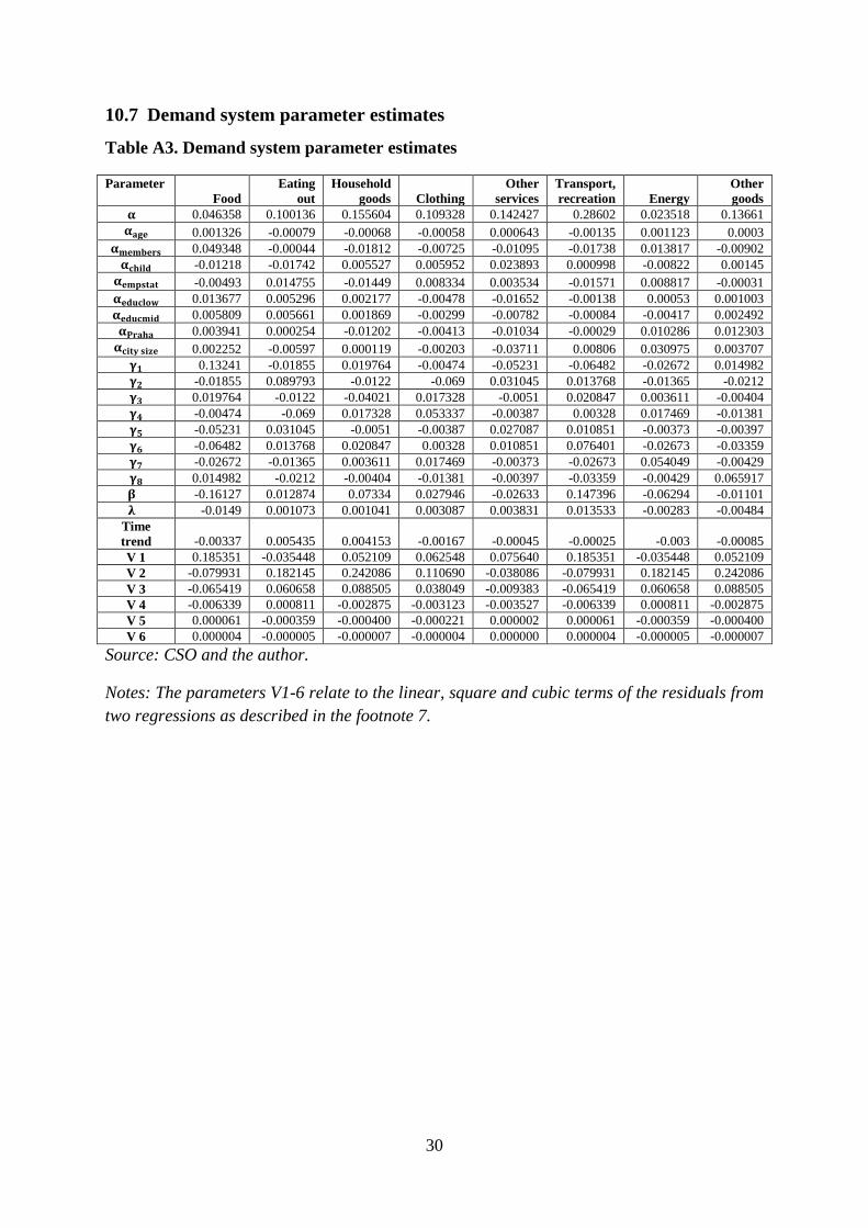
10.7 Demand system parameter estimates

Table A3. Demand system parameter estimates

Parameter

Food

Eating

out

Household

goods Clothing

Other

services

Transport,

recreation Energy

Other

goods

0.046358 0.100136 0.155604 0.109328 0.142427 0.28602 0.023518 0.13661

0.001326 -0.00079 -0.00068 -0.00058 0.000643 -0.00135 0.001123 0.0003

0.049348 -0.00044 -0.01812 -0.00725 -0.01095 -0.01738 0.013817 -0.00902

-0.01218 -0.01742 0.005527 0.005952 0.023893 0.000998 -0.00822 0.00145

-0.00493 0.014755 -0.01449 0.008334 0.003534 -0.01571 0.008817 -0.00031

0.013677 0.005296 0.002177 -0.00478 -0.01652 -0.00138 0.00053 0.001003

0.005809 0.005661 0.001869 -0.00299 -0.00782 -0.00084 -0.00417 0.002492

0.003941 0.000254 -0.01202 -0.00413 -0.01034 -0.00029 0.010286 0.012303

0.002252 -0.00597 0.000119 -0.00203 -0.03711 0.00806 0.030975 0.003707

0.13241 -0.01855 0.019764 -0.00474 -0.05231 -0.06482 -0.02672 0.014982

-0.01855 0.089793 -0.0122 -0.069 0.031045 0.013768 -0.01365 -0.0212

0.019764 -0.0122 -0.04021 0.017328 -0.0051 0.020847 0.003611 -0.00404

-0.00474 -0.069 0.017328 0.053337 -0.00387 0.00328 0.017469 -0.01381

-0.05231 0.031045 -0.0051 -0.00387 0.027087 0.010851 -0.00373 -0.00397

-0.06482 0.013768 0.020847 0.00328 0.010851 0.076401 -0.02673 -0.03359

-0.02672 -0.01365 0.003611 0.017469 -0.00373 -0.02673 0.054049 -0.00429

0.014982 -0.0212 -0.00404 -0.01381 -0.00397 -0.03359 -0.00429 0.065917

-0.16127 0.012874 0.07334 0.027946 -0.02633 0.147396 -0.06294 -0.01101

-0.0149 0.001073 0.001041 0.003087 0.003831 0.013533 -0.00283 -0.00484

Time

trend -0.00337 0.005435 0.004153 -0.00167 -0.00045 -0.00025 -0.003 -0.00085

V 1 0.185351 -0.035448 0.052109 0.062548 0.075640 0.185351 -0.035448 0.052109

V 2 -0.079931 0.182145 0.242086 0.110690 -0.038086 -0.079931 0.182145 0.242086

V 3 -0.065419 0.060658 0.088505 0.038049 -0.009383 -0.065419 0.060658 0.088505

V 4 -0.006339 0.000811 -0.002875 -0.003123 -0.003527 -0.006339 0.000811 -0.002875

V 5 0.000061 -0.000359 -0.000400 -0.000221 0.000002 0.000061 -0.000359 -0.000400

V 6 0.000004 -0.000005 -0.000007 -0.000004 0.000000 0.000004 -0.000005 -0.000007


Notes: The parameters V1-6 relate to the linear, square and cubic terms of the residuals from

two regressions as described in the footnote 7.

consumer demand system estimation and value … consumer demand system estimation and value added...

Documents