A Work Project, presented as part of the requirements for the Award of a Master Degree in

Finance from the NOVA – School of Business and Economics

ConsultingFirm - Company Valuation

António João Dinis Pereira | 24003

A Project carried out on the Master in Finance Program, under the supervision of:

Professor Fernando Anjos

4th January 2019

2

ConsultingFirm - Company Valuation

Abstract ConsultingFirm is a 5-year old fast-growing service providing company, quickly

increasing its relevance in the Portuguese market and sparking the interest from third parties.

Hence, ConsultingFirm wishes to know the market value of the company and have a simple

valuation model to be used in the future. Following an industry and value creation analysis,

the value of the company was determined through 3 well-known valuation models. Ultimately,

a valuation model for the future was developed, allowing the management to attain an

approximation of the market value of the company at any given time, through an easy but

substantiated manner.

Keywords: Finance, Equity Research, Valuation

3

Table of Contents Part I - Introduction ................................................................................................................... 5

1 | Company and Industry Overview .................................................................................. 5

A | The Company ................................................................................................................ 5

B | Competitor’s Segmentation ........................................................................................... 5

C | Industry Structure .......................................................................................................... 7

Part II – The Valuation ............................................................................................................. 8

2 | Valuation Frameworks .................................................................................................... 8

3 | Financial Statements Reformulation ............................................................................. 8

4 | Analyzing Historical Performance ................................................................................. 9

A | Return on Invested Capital ............................................................................................ 9

B | Financial Health ........................................................................................................... 12

5 | Estimating the Cost of Capital...................................................................................... 13

A | Cost of Equity.............................................................................................................. 13

B | Cost of Debt and Debt-to-Equity ................................................................................. 15

C | Weighted Average Cost of Capital .............................................................................. 18

D | Unlevered Cost of Equity ............................................................................................ 18

6 | Forecasting and Continuing Value............................................................................... 19

A | Forecasting Revenues .................................................................................................. 19

B | Projections for the IS and BS ...................................................................................... 20

C | Free Cash Flows to the Firm ....................................................................................... 20

D | Continuing Value ........................................................................................................ 21

7 | Interpreting the Results ................................................................................................ 22

A | Equity Value ................................................................................................................ 22

B | Multiples Analysis ....................................................................................................... 23

C | Sensitivity and Scenario Analysis ............................................................................... 24

D | Conclusions ................................................................................................................. 27

Part III – The Model ............................................................................................................... 28

8 | The Model ....................................................................................................................... 28

A | Intuition ....................................................................................................................... 28

B | Discussion.................................................................................................................... 29

4

List of Abbreviations

APV Adjusted Present Value

BC Business Consulting

BS Balance Sheet

CA Competitive advantage

CAPM Capital Asset Pricing Model

D/E Debt-to-Equity ratio

DCF Discounted Cash Flow

D/V Debt-to-Value ratio

EBIT Earnings Before Interest and

Taxes

EBITDA Earnings Before Interest,

Taxes, Depreciation and

Amortization

EFP Explicit Forecast Period

EV Equity value

EVA Economic Value Added

FCFF Free Cash Flow for the Firm

g NOPLAT growth

IS Income Statement

ITC IT Consulting

k Billing margin

MRP Market Risk Premium

NOPLAT Net Operating Profit Less

Adjusted Taxes

ROIC Return on Invested Capital

RONIC Return on New Invested

Capital

S&S Sensitivity and Scenario

Analysis

SG&A Selling, General and

Administrative

SO Specialized Outsourcing

WACC Weighted Average Cost of

Capital

YTM Yield to Maturity

#Proj Number of projects, in a

given business area

#h/Proj Number of hours per

project, in a given business

area

5

Part I - Introduction

1 | Company and Industry Overview

A | The Company ConsultingFirm is a Portuguese company founded in 2013, operating in

3 different business areas: Business Consulting (BC), IT Consulting (ITC) and Specialized

Outsourcing (SO).1 The first two business areas yield considerably riskier cash flows due to

executional risk and scope definition. The executional risks concern the possibility of a

deviation either in the duration or the team composition (e.g. assemble an under-skilled team)

of a certain consulting project for a client, whereas the scope definition concerns the flexibility

needed during negotiation (reflected in the billing and profit margins of each project) in order

to satisfy the client and ensure client spillover into the SO area. This area is less risky as it is

the client who bears the executional risk, therefore providing steadier cash flows with a stable

margin. The company’s revenues have been experiencing exponential growth since the creation

of the firm in 2013, having a projected value of €7.1M for 2018. After analyzing the company’s

revenues, it can be seen that the SO area is its main driver, representing approximately 62% of

the total revenues, while ITS and BC recorded 25% and 7%, respectively. The company has

currently over 20 clients, 180 company employees averaging 10 years of experience, and is

present in several industry sectors, with special remarks to the Financial sector, but also in

Retail, Utilities, Healthcare.

B | Competitor’s Segmentation By providing 3 different core consulting services,

the company is exposed to wider range competitors, tens if not hundreds, that provide the same

services. Therefore, to have a clearer idea of who are the main competitors, the companies were

subject to a filtration regarding the main service they provide, their size and age, the industries

present, and client profile. Moreover, being SO the main driver of ConsultingFirm’s revenues,

special focus will be given to the competitors in this area, as shocks driven by competition

affecting this area will impact revenues the most.

6

Some competitors, despite their big size (measured by revenues and the number of

employees) and reputation, compete with ConsultingFirm on projects that are not as complex

and usually do not require a specific know-how that clients prefer to entrust on to more

established firms. These companies include IBM (ITC), Accenture (ITC), Everis (ITC),

Deloitte (ITC and BC) and KPMG (BC), that although providing services in other areas,

compete more with ConsultingFirm on the business areas mentioned between parenthesis.

Entering the SO domain, small to medium sized firms with a similar risk profile enter the

picture, with revenues ranging from €22.8M (Mindsource, 2015) to €80M (Glintt, 2014), and

employees from 700 (Noesis) to 1.9k (Glintt). These companies include Novabase (SO and

ITC), Mindsource (SO), PrimeIT (SO and ITC), Noesis (SO and ITC), HCCM (SO), CGI

(BC and ITC), Bold International (SO) and Integer (SO). Most of these companies are

international, being present in more than one country, ranging from 5 (Glintt), 8 (Noesis and

PrimeIT) and 16 offices (Everis) across the globe. However, some are yet to begin their

international expansion (Integer and ConsultingFirm).

Depending on their experience and history providing services to a certain industry, or

even the profile and expertise of their professionals, some competitors are specialized in certain

sectors, despite having clients present in a handful of sectors. Glintt for example, is highly

regarded by clients in Pharma and Healthcare, due to the sector specific innovation and

expertise developed with different clients throughout their evolution, notwithstanding being

present in other sectors such as TMT and Financial. Another example is PrimeIT, with the IT

and TMT sectors, but being also present in Energy and Infrastructures. In view of this,

ConsultingFirm is primarily present in the Financial, Retail and Utilities sectors, along with the

presence of Novabase, Mindsource, Noesis, HCCM.

Some of these companies have their financial statements and consolidated reports

available for consulting, enabling the comparison of their performance with that of

7

ConsultingFirm, assessing the company’s strengths and weaknesses. Novabase, created in

1989, is present in the same sectors as ConsultingFirm and has several companies in its group

providing consulting services, making it a possible proxy for the industry peers as it

resembles most of them in that aspect, being also present internationally (6 offices).

Mindsource, a company also resembling Novabase regarding the sectors present and services

provided, is however different in that it is a younger (founded in 2007) and smaller firm (50-

200 employees and having €22.8M in revenues for 2018), and perhaps a better proxy for

smaller firms such as ConsultingFirm. Given the appraise from ConsultingFirm’s management

regarding the relevance of Noesis in the industry and particularly in the direct dispute for clients,

it will also be regarded as a comparable throughout the performance analysis carried on ahead.

C | Industry Structure The service providing industry such as SO, BC and ITC allow the

companies to compete on factors other than just price, where there is room for innovation and

to create a differentiated proposition. This industry structure creates the possibility to develop

strategies that rely on competitive advantages (CAs), which will be an important factor in

building ROIC and revenue growth in the industry, which will be calculated, analyzed, and then

forecasted, accounting for the ability of the company to sustain the value drivers in an industry

such as this one, wherein there is not an apparent length of product/service life cycle, since

these services are expected to remain demanded by companies, which represents a higher

chance for companies to sustain their ROIC. Especially in the Financial sector, with

developments in FinTech that are disrupting the sector, financial institutions look to increase

internal efforts to innovate and find IT solutions, incorporating technology into financial

activities and consequently improving customer service, online banking and fraud detection.2

This may constitute a potential for renewal that could allow a persistence of the CAs of firms

present in the market.

8

Part II – The Valuation

2 | Valuation Frameworks

There are several methods to value a company, each with its own different but

complementary benefits, that will be used to enrich the valuation. A particular emphasis will

be given to the Discounted Cash Flow (DCF) method, as it is a favorite among academics,

relying on cash flows and being overall an intuitive and straightforward WACC-based model.

A common concern regarding WACC-based models is that these tend to be more difficult to

apply and yield less accurate results if a company’s debt-to-value ratio (D/V) is expected to

change. The Adjusted Present Value (APV) model specifically forecasts and values any cash

flows associated with capital structure separately, rather than embedding their value in the cost

of capital (WACC), being this model more appropriate when the D/V is not expected to be

constant. Some may argue that relying solely on the cash flows of the company might provide

little insight into the company’s economic performance, since a declining free cash flow (FCFF)

can signal either poor performance or investment for the future. The Economic Value Added

(EVA) model might enlighten the valuation regarding that aspect, as it provides a yearly

analysis and focuses on the economic profit, which accounts for the opportunity cost. Lastly,

Multiples analysis, despite having a simple concept, provides an intuitive basis for precision

and helps to place the previous models in a proper context with a set of comparables.

3 | Financial Statements Reformulation

The first step in the DCF valuation is to reorganize the balance sheet (BS), labeling the

items as having an operating, non-operating, or financial capital character. This reformulation

provides the inputs necessary to calculate the Invested Capital and NOPLAT, both necessary

for the ROIC, and ultimately, the FCFF calculation, which will later be discounted to obtain the

value of operations.

9

Items regarding ‘PP&E’, ‘Accounts receivable’, ‘Tax income’ and ‘Operating cash’ are

explicitly a key component of operations. ‘Operating cash’ concerns the portion of total cash

necessary to conduct a company’s operations, which will be proxied as a percentage of sales,

as it was found that the companies with the smallest cash balances held cash just below 2% of

sales.3 Items relative to ‘Short-term deferred assets’ had to be scrutinized through the

company’s financial statement notes, whereafter the contents were separated into ‘Insurance’,

‘Rent’ and ‘Consulting projects’, all deemed operational. The same procedure was done to

‘Other assets’, which had components relative to equity investments and pension assets, both

considered nonoperational. Moving on to the liabilities, the item ‘Accrued liabilities’ was

separated into ‘Accrued salaries’, ‘Accrued projects’ and Other accrued liabilities’, wherein the

first two were considered operational as they are tied with the company’s activity, whereas

‘Other accrued liabilities’ was considered financial as its value is related to other debtors and

forms of debt. The item ‘Partners’ was considered a debt equivalent since its value concerns

credit from the firm’s partners, hence labeled financial. After safeguarding that the sources of

the total funds invested matches the use of the total funds invested, Invested Capital and

NOPLAT were calculated, having a first glimpse at the ConsultingFirm’s ROIC since its

foundation in 2013. The same process was done to the competitors Noesis, Mindsource and

Novabase.

4 | Analyzing Historical Performance

A | Return on Invested Capital ConsultingFirm’s historical performance will now be

analyzed and compared with that of its selected peers, Noesis, Novabase and Mindsource.

Despite having some information available to the public, some of the competitor’s financial

statements and notes are either not available in certain years, or incoherent in terms of the

segregation done to its items throughout the reports. Nonetheless, the information available was

gathered and processed in order to compute the ROIC for each of the competitors for the sake

10

of this comparison. This calculation will also enable the 2-level ROIC decomposition and

analysis, to build a broader view of the company’s operating performance. Lastly, the

company’s financial health will be assessed to determine whether it possesses the financial

resources to conduct business and make short and long-term investments.

In the Table 1, it can be seen the ROIC summary for ConsultingFirm and its

competitors. Novabase’s ROIC was calculated without Goodwill, to only measure the

underlying operating performance, being this discussion present in Appendix 1.

ConsultingFirm’s ROIC reached above normal results in its first years due to the small amount

of Invested Capital needed to start operations but is now naturally decreasing into a ROIC of

17.4%, resembling more an industry average. As expected in an industry such as this one, ROIC

values tend to be high, ranging from 10% to 20%, mirroring the results present in the analysis

done on ROIC across industries in the United States.4 These factors can also be used to

understand ConsultingFirm’s revenues growth since its foundation (Appendix 3), which is

naturally decreasing but still reaching values higher than the competitor’s average. Novabase

has been decreasing its Invested Capital with not so significant impacts on NOPLAT, causing

a stable increase in ROIC, reaching 33.3% in the last year, caused by an enormous decrease in

‘Trade and other receivables’ that led the Invested Capital to decrease more than usual. Noesis

has been registering shyer values of ROIC, from 10-15%, having now reached a steadier

NOPLAT, possibly due to the decrease in Invested Capital registered in 2014.

Looking at a first level decomposition of ROIC present in Appendix 4 and Graphic 1,

it can be seen that ConsultingFirm’s profitability, measured by the ability to generate profit

2012 2013 2014 2015 2016 2017

ROIC

ConsultingFirm NA NA 121,3% 47,1% 22,8% 17,4%

Noesis NA 4,7% 15,7% 15,5% 12,3% NA

Mindsource 23,5% 233,4% 14,7% 5,2% NA NA

Novabase (w/o Goodwill) NA NA 9,0% 12,4% 18,8% 33,3%

Table 1 | ConsultingFirm and competitor’s ROIC.

11

from each unit of revenues, has been decreasing (from 7.6% to 4.8%) despite the reduction in

SG&A costs, mainly due to the increase in employee related expenses over the registered

period, that were able to be stabilized in the last year, being therefore ConsultingFirm’s

profitability expected to increase and be more efficient if this stabilizing ability is repeated.

This aspect of ConsultingFirm’s profitability is not seen in its competitors, as all have a portion

referring to SG&A costs of 20-30% and Employee costs of 60-70%, whereas ConsultingFirm

has more balanced values, 40-60% for SG&A costs and 35-50% for Employee costs.

ConsultingFirm’s SG&A expenses include fees, subcontracts and transportation, which all have

been decreasing, excepting for fees. As expected, Novabase and Noesis incur costs of the same

nature, all ranging from commission and consultancy fees, to transportation and other

specialized services such as advocacy and accounting. Noesis registers similar profitability

margins, despite upward trending. Mindsource had values around 5% which dropped to

approximately 2.5% in the last registered years.

Regarding ConsultingFirm’s capital turnover, representing the revenue by each unit of

capital invested, it is higher than the competition given the recent foundation of the firm, but is

Graphic 1 | Comparison between the ROIC levels of profitability, capital turnover, and fiscal, in

each company’s last recorded year.

12

unavoidably decreasing due to the increase in working capital incurred to operate. Nonetheless,

ConsultingFirm reaches a value of 548.5% in the last year, explained partially by the low

amount of PP&E and the inexistence of intangibles, which is not found in the competitors. The

aforementioned drop in Novabase’s ‘Trade and other receivables’ item explains the above

normal value of capital turnover of 514.7%, which deviates from the company’s trend in prior

years of 215-315%.

Lastly, looking at the fiscal part of this decomposition, it can be seen the impact in ROIC

from the ability to minimize operating taxes, given by 1-Operating Tax Rate. ConsultingFirm’s

value of 65.9% resembles that of its direct comparable Noesis (69.8%). The two remaining

companies, Novabase and Mindsource, display significantly higher (86.9%) and lower (35.2%)

values, respectively. Given the lack of nonoperational elements in the EBITDA and EBIT, this

value is not expected to vary significantly from the recorded values.

B | Financial Health Part of any valuation exercise is to assess the company’s financial

health and how robust its financial structure is, from an investor’s point of view. With that in

mind, both liquidity and leverage were analyzed as a way of figuring out the firm’s capacity to

meet its short and long-term obligations. The entire analysis can be seen in Appendix 5. The

key conclusion is that ConsultingFirm is financially stable in the short and long-term, despite

relying heavily on its account receivables and the ability of clients meeting their payments,

hence having some executional risk in the short-term. Adding the already existent concern

surrounding clients being often overdue on their payments, conveyed by the CFO and

mentioned briefly at the end of this analysis, there is room for a situation of distress that should

be acknowledged and acted upon. Possible measures are also discussed in the analysis in

Appendix 5, replicating competitors such as Novabase, who despite having a healthy short-

term equilibrium, are not so dependent on receivables.

13

5 | Estimating the Cost of Capital

When valuing a company using the DCF method, the forecasted FCFF are discounted

by the WACC. The WACC represents the opportunity cost that investors face for investing their

funds in one particular business instead of others with similar risk, being therefore also

interpreted as the required return for each investor. To determine the WACC it is needed the

cost of equity, the after-tax cost of debt, and the company’s target capital structure, which

must be estimated through models that proxy the expected return on alternative investments

with similar risk using market prices.

A | Cost of Equity The cost of equity will be estimated using the Capital Asset Pricing

Model (CAPM), since it is the most commonly used model for cost of equity estimations.

However, other models could have been used, such as the Fama-French three-factor model and

the Arbitrage Pricing Theory Model (APT), which differ mainly in their definition of risk. The

cost of equity is built on the risk-free rate, the market risk premium (MRP), and a company-

specific risk adjustment (given by the beta in the CAPM), all present in CAPM’s Security

Market Line in the following manner 𝐸(𝑅𝑖) = 𝑟𝑓 + 𝛽𝑖 ∗ 𝑀𝑅𝑃. The risk-free rate is usually

estimated using government default-free bonds since these securities, although not necessarily

risk-free, have extremely low betas. There is a debate regarding the bond maturity that should

be used, since longer-dated maturities might reflect the cash flow stream better, but their

illiquidity implies changes in the prices and yield premiums, which may not reflect value at the

moment. The 10-year bond is usually the preferred maturity as it finds an equilibrium in this

tradeoff between the fitting of the company’s cash flows and the bond liquidity. The 10-year

German Bund could be chosen for this proxy, having a yield of 0.46% as of October 2018.

However, being ConsultingFirm a young company, a longer period might be recommended to

better capture the growth path and age of the company. Hence, the 30-year German Bund will

be chosen as the risk-free for the model, which is currently yielding 1.04%.

14

Secondly, the MRP, given by the difference between the market’s expected return and

the risk-free rate, can be estimated through various models, being the method selected the

measurement and extrapolation of historical returns. This method lies on the assumption that

the level of risk aversion has not changed over the past years, making the historical excess

returns a reasonable proxy for future premiums. Hence, data relative to the Euro Stoxx 50 and

the 10-year German Bunds was collected for the longest period available, from December 1986

to January 2018, with the goal of reducing estimation error as much as possible. These two data

sets were selected as the market and risk-free proxies and were used to calculate the annualized

return of the market and average risk-free rate, which enable the estimation of a MRP of 5.83%

(Appendix 8). The debate surrounding the MRP and its possible values is never-ending, being

the interval considered by academics and practitioners between 4% and 6%. Given the period

considered for the calculations (1986-2018) and the possibility of the presence of noise in the

estimations, a 95% confidence interval was calculated, seen in Appendix 8, setting the MRP to

a value between 4.86% and 5.74% with 95% confidence. Moreover, looking at KPMG’s Equity

Market Risk Premium Research Summary, it can be seen that the recommended value for the

MRP is 5.5% as per 30 June 2018, value that falls in the interval being considered and backing

the initial estimate of 5.83%.5

Lastly, regarding the company beta, the common method of regressing the return of the

company’s stock with the market’s return to calculate the raw beta is not possible here since

ConsultingFirm is not publicly traded. In cases such as this one, the proceedings often entail a

gathering of a group of public comparable companies, such as Novabase, Accenture, Tata

Consulting Group, Capgemini, Cognizant and CGI, in order to obtain an industry unlevered

beta, that could be relevered using ConsultingFirm’s target debt-to-equity ratio (D/E) and find

the company’s beta. However, thanks to Professor Aswath Damodaran’s public collection of

datasets regarding several valuation and corporate finance topics, it is possible to gather

15

information about a much bigger set of comparables. Information concerning two industries

was collected: Computer Services and Business&Consumer Services.6 The first set has

information on 111 companies from all over the globe, including all the 6 companies previously

mentioned, as well as several other service providing IT companies, whereas the second set has

169 companies, several of which in the business consulting and outsourcing areas. Hence, in

order to weigh the different business areas, an average between the two was done, that resulted

in an average industry beta of 0.88, which then relevered using ConsultingFirm’s target D/E,

yields a company beta of 0.91 (Table 2). For comparison’s sake, the unlevered betas of the

mentioned companies were manually calculated using monthly data of the past 5 years, having

an acceptable minimum of 60 data points while avoiding high-frequency beta estimations, often

unreliable due to the bid-ask bounce distortion. The results can be seen in Table 2, signaling

the approval of the collected beta from Damodaran’s datasets.

Finally, the cost of equity can be estimated, by entering the calculated values for the

risk-free, MRP and company beta in the equation 𝐸(𝑅𝑖) = 𝑟𝑓 + 𝛽𝑖 ∗ 𝑀𝑅𝑃, yielding a value of

6.32%.

B | Cost of Debt and Debt-to-Equity Having now the cost of equity, the next step is to

estimate the cost of debt. For investment-grade companies, the yield to maturity (YTM) of the

company’s long-term bonds is normally used as a suitable proxy since it is immaterial to

consider the risk of default in these bonds. However, ConsultingFirm does not have publicly

traded debt through which the YTM can be extrapolated, nor does it have a credit rating as the

β Summary Damodaran Damodaran Novabase Accenture Tata CS Capgemini Cognizant CGI

βe (levered) 1,17 1,10 0,46 0,72 0,62 1,20 1,05 0,51

D/E 0,27 0,31 0,22 0,00 0,01 0,48 0,08 0,28

βu (unlevered) 0,92 0,84 0,37 0,72 0,62 0,81 0,98 0,40

0,97 0,89

Industry βu 0,88

ConsultingFirm's Target D/E 0,03

Consulting Firm's proxied βe 0,91

Note: The information regarding the D/E of each company was taken from the respective company's financia l report (l ink in Excel )

Table 2 | Summary table of the beta calculations.

16

ones provided by professional rating agencies such as Standard & Poor’s and Moody’s, which

could be used to compare YTMs on portfolios of bonds with the same credit score. These

characteristics of ConsultingFirm constitute a barrier to the direct calculation of the cost of debt,

which will have to be computed through an indirect method.

Since credit ratings are only available for large corporations, the credit risk of small and

medium firms can be assessed through models of credit scoring that rely on information present

in the BS and macroeconomic data. One of those credit scoring models is the Z-score,

developed by Edward Altman (1968).7 Altman’s Z-score and its variations (Z’’ and Z’’s-score)

determines if a public or private firm is in a safe or distress zone, by using different financial

ratios, as can be seen in Appendix 9. After calculating the Z’’s-score for ConsultingFirm

(Appendix 10), it can be interpreted that the company has been improving its position in the

safe zone regarding credit concession (8.67 far exceeds the safe zone threshold of 5.85). Using

this value, an empirical match between Z-scores and observed ratings can be done, present in

the table in Appendix 11, which normally is used to get the probability of default associated

with such rating, but in this case will be used to get the YTM.8 From this table, it can be inferred

that ConsultingFirm’s rating is equivalent to a AAA or Aaa. This rating might be

overoptimistic, but it results from ConsultingFirm’s assets being largely operational and a lack

of non-current assets, which drive the financial ratios upward. It also seems to fit the industry’s

values for Z’’s-score, present in Appendix 12, as well as D/V of 54.39%.

There are now two methods of determining the so sought YTM. One way is to use the

table in Appendix 13, where it can be seen the yield spread over U.S. Treasuries by Bond

Rating. Although this table is outdated (from May 2009) and concerns U.S. Treasuries, it was

the most recent set of data available and will still be used for context and to help calibrate

results. The risk-free, proxied by the German 10-year bund yield, will be added to the value of

0.58% taken from the foregoing table, totaling a YTM and cost of debt of 1.04%. Given the

17

increased possibility of inaccuracy from using the table from the last method, another existent

method is to use the YTM on a security with the same credit rating. For comparative purposes,

it was collected data beyond Aaa-rated corporate bonds, that is present in Appendix 14. The

data captures corporate bonds from Germany, France and the Netherlands, all traded in euros

in order to match the cash flows from ConsultingFirm. As a more conservative measure, the

average of these corporate bonds was done to estimate the cost of equity of ConsultingFirm, as

the actual rating of the company might not be that high, also capturing the liquidity risk

mentioned in the financial health analysis. Hence, the estimated cost of debt of

ConsultingFirm will be 1.12%, which resembles the value of 1.04% derived from the previous

method.

In the WACC formula the D/E is at market value, being this the last input needed.

Looking first at the recorded D/E ratio (accounting value), in the last 3 years (2015, 2016 and

2017) the D/E was 0.93, 0.83 and 1.19, resulting in a respective D/V of 0.48, 0.45 and 0.54.

Given the difficulty of translating the target D/E into market value for the case of

ConsultingFirm, for the reasons already discussed, and that ConsultingFirm has not a defined

ratio for the future, Damodaran’s data was again consulted, this time concerning the D/E ratios

at market value for the same industries considered in the beta estimation (Computer Services

and Business&Consumer Services), which yielded values for the D/E of 30.83% and 27.44%,

respectively.9 Another way to interpret the target D/E is as the value of D/E that will be inherent

of the company’s capital structure in the future, and this value can be calculated using the Equity

value (EV) and debt values seen in Table 4. If a value of target D/E of 1 is used, then the value

of D/E given by the model is approximately 0.03 (€0.5 million in debt divided by an EV of

€17.5 million). Hence, by using this circularity and inputting values for the D/E and registering

back the values given by the model, the optimal value for D/E can be searched for, being that

value the one that registers an equilibrium, by being the same in both ends. Hence, the value

18

chosen for the target D/E will then be 0.03. Using a value for the target D/E resembling

Damodaran’s benchmark values of roughly 30% will result in a different in EV, under the DCF,

of approximately 2%, hinting on the EV’s sensibility to the target D/E, an aspect that will be

further discussed in the sensitivity analysis.

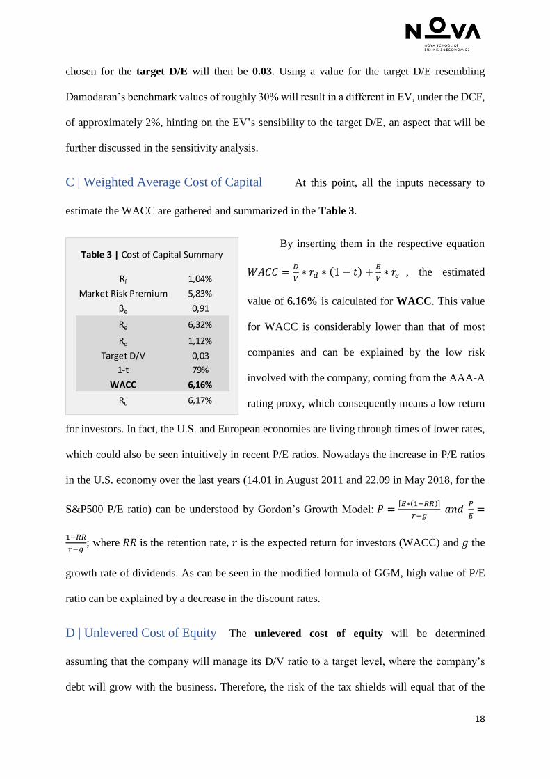
C | Weighted Average Cost of Capital At this point, all the inputs necessary to

estimate the WACC are gathered and summarized in the Table 3.

By inserting them in the respective equation

𝑊𝐴𝐶𝐶 =𝐷

𝑉∗ 𝑟𝑑 ∗ (1 − 𝑡) +

𝐸

𝑉∗ 𝑟𝑒 , the estimated

value of 6.16% is calculated for WACC. This value

for WACC is considerably lower than that of most

companies and can be explained by the low risk

involved with the company, coming from the AAA-A

rating proxy, which consequently means a low return

for investors. In fact, the U.S. and European economies are living through times of lower rates,

which could also be seen intuitively in recent P/E ratios. Nowadays the increase in P/E ratios

in the U.S. economy over the last years (14.01 in August 2011 and 22.09 in May 2018, for the

S&P500 P/E ratio) can be understood by Gordon’s Growth Model: 𝑃 =[𝐸∗(1−𝑅𝑅)]

𝑟−𝑔 𝑎𝑛𝑑

𝑃

𝐸=

1−𝑅𝑅

𝑟−𝑔; where 𝑅𝑅 is the retention rate, 𝑟 is the expected return for investors (WACC) and 𝑔 the

growth rate of dividends. As can be seen in the modified formula of GGM, high value of P/E

ratio can be explained by a decrease in the discount rates.

D | Unlevered Cost of Equity The unlevered cost of equity will be determined

assuming that the company will manage its D/V ratio to a target level, where the company’s

debt will grow with the business. Therefore, the risk of the tax shields will equal that of the

Table 3 | Cost of Capital Summary

Rf 1,04%

Market Risk Premium 5,83%

βe 0,91

Re 6,32%

Rd 1,12%

Target D/V 0,03

1-t 79%

WACC 6,16%

Ru 6,17%

19

operating assets (𝑟𝑢 = 𝑟𝑡𝑥𝑎). With this simplification, the unlevered cost of equity can be solved

for in the following equation 𝑟𝑒 = 𝑟𝑢 +𝐷

𝐸∗ (𝑟𝑢 − 𝑟𝑑), yielding a value of 6.17%, that can also

be seen in Table 3.

6 | Forecasting and Continuing Value

Having the financial statements prepared, the next step is to develop a set of financial

forecasts that reflect ConsultingFirm’s expected performance. This will provide the information

needed to compute the FCFF. The explicit forecast period (EFP) is from 2019 to 2030, long

enough for the company to grow and earn at a constant rate.

A | Forecasting Revenues The first and critical step is to forecast revenues, since

many accounts will be forecasted as a percentage of it. The forecast was done resembling a

bottom-up approach, breaking the revenue components, analyzing their historical values, and

projecting each one considering expected demand. Revenues were separated by business area

(BC, ITC and SO) given their differences in weight, the way business is conducted, and plans

for the future. Each business area was then broken down, detailing the billing margin (k) and

the number of hours spent in projects for the years, which depends on the number of projects

(#Proj) and the average number of hours per project (#h/Proj), representing the latter the

complexity of an average project. After processing a set of raw data regarding the details of

each project done since July 2015, it was possible to obtain the inputs mentioned for each

business area, being in Appendix 15 the table for the BC area and a summarized table for all

areas. The difference between the values of revenues given by multiplying k by the number of

hours, and the recorded revenues, concern software sales done (also seen in the ‘Cost of Sales’)

and extra-hours not registered, being the difference between the two in the recorded years 1%-

5% of the actual recorded revenues for the year. For the first 5 years of the forecast, the CEO

offered insight on what values the revenues are expected to take, along with the plans regarding

20

the future billing for each business area and the expected path on the undertaking of new

projects and their foreseeable complexity (see ‘Revenue’ notes in Appendix 16), allowing for

the completion of the revenues forecast.

B | Projections for the IS and BS The financial statements were then completed,

being the reasoning behind each projected item explained in the notes in Appendix 16 and

Appendix 17, for the IS and BS respectively. Given the circularity problem between these two

financial statements, the items responsible for establishing the accounting equilibrium going

forward are going to be ‘Newly Issued Debt’ and ‘Excess Cash’. These two accounts will

depend on the total value of assets (excluding ‘Excess Cash’), and the total value of liabilities

(excluding ‘Newly Issued Debt’) plus Equity. If the total assets are greater than the sum of

liabilities and equity, then the difference will go ‘Newly Issued Debt’, whereas if total assets

are smaller, it will go to ‘Excess Cash’, hence ensuring the accounting equilibrium.

C | Free Cash Flows to the Firm Now it is time to build the FCFF and free

cash flow available to investors, reconciling the latter with the cash flow received from

investors. The first component calculated is the gross cash flow, which represents the cash flow

available for investment generated by ConsultingFirm’s, calculated by adding the NOPLAT to

depreciation. Next, the gross investment must be subtracted, which in the case of

ConsultingFirm is only given by the change in operating working capital (OpEx) and net capital

expenditures (CapEx), both growing in the EFP, reflecting the expected growth of the company.

After doing this subtraction, the FCFF is obtained, which is the stream of cash flows used in

the valuation of operations and the core of the overall valuation. This stream of cash flows

achieves high growth in the first years of the EFP with tendency to decrease as time passes,

stabilizing at 7% in the last two years of the EFP, being expected to further decrease to values

approximating the growth of the economy. Although not included in the FCFF, the cash flows

21

related to non-operating assets have value and are evaluated separately and then added to the

FCFF to give the total free cash flow available to investors. To ensure that the procedures were

technically correct and avoid mistakes, the cash flow available to investors should be identical

to the total financing flow, an important reconciliation that is checked for in the Excel

calculations.

D | Continuing Value The value of the firm has two components: the present value of

the FCFF during the EFP, and the present value of the cash flow after the EFP, being the latter

the continuing value. A considerate estimate of the continuing value is fundamental because

this term often accounts for a large percentage of the company’s value, as most of a company’s

value will be created in the continuing-value period. In the DCF model, continuing value is

estimated using the value driver formula 𝐶𝑉𝑡 =𝑁𝑂𝑃𝐿𝐴𝑇𝑡+1∗(1−

𝑔

𝑅𝑂𝑁𝐼𝐶)

𝑊𝐴𝐶𝐶−𝑔, where 𝑔 is the expected

growth rate in NOPLAT in perpetuity.

For the growth rate in NOPLAT it is usually assumed that in the future it will be identical

to the forecasted value for the long-term growth rate of the economy, since few companies can

be expected to grow faster than the economy for long periods.10 According to Banco de

Portugal’s estimate, the long-term growth rate of the economy is going to be 1.7% in 2020, the

longest projection available.11 Although ConsultingFirm is a young and fast-growing company

with a steady-state growth of FCFF of 7%, given this common perpetuity assumption and the

fact that growth is more difficult to sustain than ROIC as a company grows, 𝑔 will be assumed

to equal the growth rate projected for the Portuguese economy of 1.7%.

Having calculated the WACC in the previous chapter, the focus now lies on the RONIC.

Although the RONIC in the value driver formula represents the value that ROIC will gradually

approach, in some industries RONIC and ROIC differ and are not necessarily equal. In

Appendix 18 it can be seen the ROIC evolution in the EFP and that ConsultingFirm reaches a

22

steady-state value of ROIC of 19%. This value will be the one considered for the value driver

formula, as it is the steady state value and is in the industry average of 15%-20%, which is

important since individual company ROICs gradually tend toward their industry medians over

time. Moreover, high-ROIC companies tend to maintain their high returns on invested capital,

with a 75% probability of either remaining in the 10%-20% or even increasing to >20%.12

7 | Interpreting the Results

A | Equity Value Finally the company’s Equity value (EV) as of 2019 can be calculated

under the several methods used, by subtracting the value of net debt of 2019 to the Enterprise

value, calculated by adding the value of operations with the value of nonoperations of 2019.

In Table 4 can be seen the valuation table for the DCF method, which yields an EV of

approximately €17.8 million, 19.6% of which coming from the EFP, while 83.4% coming from

the continuing value formula. The EVs under the several methods should yield identical or

similar results, being the variation registered among all below 1% of the total value. Through

the EVA method (Appendix 19), it is possible to see the yearly economic profit, which contrary

to accounting profit, accounts for opportunity cost. In fact, in the EFP, over the next 12 years,

the economic profit is expected to be €5.6 million, wherein the weight of the continuing value

of economic profit in the EV (63.3%) is less than the value registered in the DCF and APV

Table 4 | DCF Valuation table. Table 5 | APV Valuation table.

Value of Operations 3 508 246 €

Value of nonOperations 9 528 €-

PV of Continuing Value 14 992 267 €

Continuing Value2029 28 930 784 €

NOPLAT2030 1 416 562 €

g (NOPLAT growth) 1,7%

RONIC 19,0%

WACC 6,16%

Total Enterprise Value 18 490 984 €

Net Debt 593 331 €

Equity Value 17 897 654 €

Unlevered Cost of Equity 6,17%

PV of FCF 3 506 662 €

PV of ITS 82 306 €

PV of Continuing Value 14 981 671 €

Value of Operations 18 570 638 €

Value of nonOperations 9 528 €-

Enterprise Value 18 561 110 €

Net Debt 593 331 €

Equity Value 17 967 779 €

23

methods. Finally, looking at the APV method (Table 5), it can be seen the value coming from

the financing benefits, despite the company having a constant D/E ratio. The present value of

tax shields amounts to approximately €0.082 million, whereas the present value of the FCFs in

the EFP as if all equity financed amounts to €3.507 million, similar to the value of operations

in the same time period under the DCF. It is important to highlight that this model although

accounting for the benefits of having debt, does not account for the financial distress costs that

come with high levels of debt (M&M).

B | Multiples Analysis The usual complementary multiples valuation was also conducted

to triangulate the results, which can be seen in Appendix 20. Despite being knowingly limited

and simplistic, it still is widely used as the accuracy of any analysis relies on that of the forecasts

made. Professor Damodaran’s data tables will once again prove to be both helpful and suitable,

this time for consulting the information regarding the multiples chosen: Enterprise Value/Sales

and Enterprise Value/EBITDA.13 Recreating the process done for the beta calculation, the

values for the Computer Services and Business&Consumer Services industries were withdrawn

and then averaged, yielding an Enterprise Value/Sales and Enterprise Value/EBITDA multiples

of 1.64 and 11.75, respectively. These values, multiplied by the 2019 value of sales and

EBITDA produce an EV of approximately €13.5 million and €8.15 million, which

underestimate the company value by 24.61% and 54.43%, according to the values computed

through the valuation methods (€17.8 million). A possible explanation for this disparity could

stem from the fact that the benchmark’s implicit g is lower than that of ConsultingFirm. On

average, the companies in Damodaran’s data sets are going to be more mature, with implicit

growth rates lower than that of ConsultingFirm, a young and fast-growing company. Therefore,

evaluating ConsultingFirm with such multiple causes the company to be undervalued. In fact,

this is a known limitation of Multiples valuation, where by simplifying complex information

into a single value, factors that affect the company’s intrinsic value, such as growth, are

24

disregarded. A greater insight on this possible understatement will be enabled by a sensitivity

and scenario analysis that will be conducted, signaling that the perhaps variations in variables

are more likely to be of a negative character.

C | Sensitivity and Scenario Analysis Part of any interpretation concerns a Sensitivity

and Scenario analysis to test how the company’s value responds to changes in key inputs and

assess several possible scenarios, ultimately bounding the valuation range. The inputs chosen

come from the IS (revenues, SG&A, employee costs, and income taxes), the BS (receivable

period, target D/E ratio, debt and invested capital), the continuing value formula (WACC, g and

RONIC), and from the cost of capital (risk-free, MRP, beta, cost of equity and cost of debt).

These inputs were subject to 1%, 2.5%, 5% and 10% changes, followed by an analysis of the

impact on the EV percentagewise.

As it can be expected, changes in revenues have a considerable impact in the EV, more

concretely, a 1% change in this variable causes an almost equal impact of 0.9% in EV, being

this 1:0.9 relation verified along the range considered (see Appendix 21). Given the

mathematical formula through which the revenues for each business area are forecasted

(𝑏𝑖𝑙𝑙𝑖𝑛𝑔 𝑚𝑎𝑟𝑔𝑖𝑛 ∗ # 𝑜𝑓 𝑝𝑟𝑜𝑗𝑒𝑐𝑡𝑠 ∗ # 𝑜𝑓 ℎ𝑜𝑢𝑟𝑠 𝑝𝑒𝑟 𝑝𝑟𝑜𝑗𝑒𝑐𝑡), a percentage increase in any

one of the three components has the same impact on the business area’s revenues independently

of which one it is, having its impact carried entirely. Changes in these components in the SO

area will affect EV the most, causing a 4.4% change in EV from a 10% change in the variables.

Looking at the variations in the costs (Appendix 21), these have the biggest impact in the EV.

In fact, just a 1% change in Employee Expenses and SG&A costs causes a negative variation

in the EV of 11.5% and 6.4%, respectively. To understand this, it is important to remember that

these two costs account for more than 90% of ConsultingFirm’s operational costs. Adding to

the fact that the company does not have any cost of sales and has nearly insignificant other

gains (government subsidies) and expenses (tax related), SG&A and Employee costs become a

25

major share of the company’s EBITDA and EBIT, which affect NOPLAT and consequently

the FCFF, explaining the enormous sensitivity and impact these two costs have on the EV.

Moving on to the BS, the only item with a material impact in the EV is the

average receivable period (Appendix 22), which will be subject to a more thorough analysis

ahead. A 10% increase in this item will result in a decrease of 5.4% in the EV, while all the

other items do not surpass the 0.1% mark. Translated in days, if instead of the 115-day

receivable period that was forecasted, the 90-day period was satisfied, the impact in EV would

be of 12.02%. Even a decrease to 100 days would generate an increase of 7.19% in the EV.

Regarding the components of the continuing value formula, both the 𝑔 and the 𝑅𝑂𝑁𝐼𝐶 have

a small impact on the EV (2.5% and 0.8% increase for a 10% variable increase, respectively),

being the WACC the most impactful variable. In fact, when increased 1%, 5% and 10%, the

cost of capital will have a negative impact on the EV of 1.8%, 8.3% and 15.5% (Appendix 23),

signaling the importance of a well estimated WACC in order to avoid variations in the EV

coming from estimation and proxy inaccuracies. Some of the components of the cost of capital

are estimated with less certainty than others, being therefore helpful this analysis to perceive

whether the uncertainty can significantly affect the EV estimated. As can be seen in Appendix

24, a 1% increase in the cost of equity will result in a decrease in the EV of 1.7%, being the

main drivers of that variability the company beta and the MRP, both causing decrease of 1.4%

in the EV for the same 1% increase. The risk-free rate and the cost of debt will have a much

less substantial impact, with a 2.8% and 0.1% decrease, respectively, for a 10% increase of the

variable.

There were 3 scenarios considered for the scenario analysis: an optimistic and

pessimistic analysis, where the variables in question are the revenues and the average receivable

period, analyzing their impact together; the impact in the EV of several combinations (shifts of

5%) of g and WACC, and RONIC and g; and the tradeoff approached in chapter 1A regarding

26

variations in the k of BC and ITC, in function of the #Proj of the SO area. In the first scenario,

both revenues and receivables were changed in order to mimic a crisis scenario, where not only

the revenues decrease, but clients struggle more to comply with their deadlines. In fact, a 5%

decrease in revenues and 5% increase in the average receivable period will cause the EV to

decrease by 7.05%. In case of an economic boom, the impact will have the same size but will

be positive.

In the Appendixes 25 and 26 it can be seen the percentage changes in the EV from

different combinations of g and WACC, and RONIC and g. The goal is to analyze different

joint scenarios of higher or lower long-term growth, risk, and value creation. Looking at the

values displayed in the first graphic (Appendix 25), one of the conclusions withdrawn is that

with higher WACC, the impacts in the EV of changes in g are smaller, meaning that when the

WACC is lower (by 10%), an increase in g (by 10%) results in a positive impact of 24.4% in

EV, whereas if the same g increase is registered against a much higher WACC (by 10%), the

EV will decrease by 17.1%, which in absolute terms is not as big as a shift of 24.4%. This

means that for companies with a lower WACC, such as ConsultingFirm, a more robust

estimation for g is recommended. Another conclusion regards the strength of each variable.

Although a lower than estimated g can be offset by an also lower than estimated WACC,

represented in the positive third quadrant, the same cannot be said for a higher than estimated

g, which is not enough for a positive change in the EV when the WACC is also higher than

estimated, represented in the negative first quadrant. Looking at the Appendix 26, it can

immediately be concluded from the values shown that impacts in the EV are less significant

than those of the previous graphic. Furthermore, negative combinations of these two variables

have a smaller impact than positive combinations. A 10% decrease in g and RONIC causes a

decrease in EV of 3.1%, whereas an increase of 10% on the same variables only increases the

EV by 3.3%. The changes are not massive but are worth noting.

27

Finally, regarding the tradeoff from the scope limitation of chapter 1A, it can be seen in

Appendix 27 a graphic that can be used to draw some conclusions. Given the way the revenues

are computed, for equal percent changes in the variables considered, the EV would not change.

The relevant quadrants are highlighted in grey, which convey that perhaps being highly flexible

in the billing margin to clients (k) in the BC and ITC areas to ensure client spillover to the SO

area is not that beneficial as it seems. In fact, if ConsultingFirm is less flexible in the billing

margin, reflecting an increase in 5 percentage points (e.g. from 30% to 35%) and resulting in a

decrease of the number of projects in SO (e.g. from 15 to 10 projects), the EV would increase

3.9%, whereas if ConsultingFirm is more flexible it will be deteriorating value (-3.9%).

However, a disadvantage with this particular analysis is that it is not possible to know the size

of the decrease in the number of projects in SO in response to a change in the billing margin.

D | Conclusions ConsultingFirm’s dependence on its receivables (liquidity) and how that

can be worsened by the clients not paying on time is a worrisome conclusion from this project.

In fact, in a scenario of economic crisis, not only would the company’s revenues be affected,

but also the clients’ revenues, causing an increase in the average receiving period, having now

two variables affecting the EV substantially (7.05%), as analyzed in the first scenario. This

dependence on the receivables could be softened by replicating Novabase’s BS structure and

have nonoperational assets, such as investments and/or excess cash in its BS.

One of the setbacks encountered during the project was the inability to forecast the

Employee costs using the company data regarding its employees, as it was explained in

Appendix 16. The solution was to forecast the account using revenues, which is the next best

option, despite being less accurate and the source of big variations in the EV. Despite this,

Employee costs and SG&A costs were sought to be forecasted in a robust manner, having the

sum of its percentages in terms of Revenues always around 90%, value that is common to

ConsultingFirm and its competitors. Regarding the valuation and the EV, there are variables

28

that affect greatly the EV obtained (namely Revenues, SG&A, Employee costs, and WACC),

discussed in the S&S analysis, being particularly crucial to have a robust estimation of those

variables. A particularly thorough estimation of those variables was sought throughout the

project, being recommended to be carried on as much as possible when estimating EV at some

point in the future.

Part III – The Model

8 | The Model

A | Intuition

This model is to be the basis of a management model, as it allows the managers to more

accurately provide employee benefits, serving as a proxy for stock options, and to aid in

properly assessing proposals for the company. The model developed here aims to give an

approximation of the EV of the firm at a given time, disregarding the items analysis, thorough

research and computations, and overall scrutiny put into the valuation model built throughout

the project. This simplicity is achieved by relying on that model, demanding only a few crucial

inputs to obtain the EV, as can be seen in Appendix 28. The user of the model is guided through

several notices while inputting the projected values.

The most important of those inputs are the parameters that build up each business area’s

revenue, namely the #Proj done, the average #h/Proj, and k, which need to be inserted for the

year 0 (current year), upon which the growth forecasts will be made, through the selection of

the expected growth for the first and last 5 years of the 10-year forecast period, or simply by

directly inputting the values. The other inputs concern the most relevant components of the cost

of capital (company beta and target D/E) and continuing value (NOPLAT growth and RONIC).

It is not needed to calculate any more items, either because they are forecasted as a function of

the projected revenues or simply because they are immaterial and not worth the attention. All

29

the transformations done to the financial statements throughout the project are now done

automatically in the new model, which immediately displays the new EV.

B | Discussion

There are a few drawbacks that come from the model’s simplicity. Optimally, the

model’s “engine” would be updated, adjusting for new forecasts that might change with time

and as the company collects more information, for example regarding the percentage of

revenues that Employee and SG&A costs represent. In fact, if not adjusted, this model will tend

to be more inaccurate as years go by, since the company is also going to develop and more

accounts are going to be created in the financial statements. To try and prevent this issue, a few

notes are going to be present in the report given to de company about the model, explaining

how to do these updates in the model’s “engine” when needed.

Moreover, being this model a Value Based Management (VBM) instrument, from an

economic point of view, there are certain implications of using such a model for strategic and

operating decisions that could lead to unwanted results. Namely, the inputs are subject to the

user’s criteria, which could result in a form of perverse incentives. However, this conflict of

interests could be mitigated by having certain inputs, which have a great impact on the EV,

such as the cost of capital and continuing value components, controlled by having their freedom

removed. These inputs could be set to be extracted from Damodaran’s datasets, for example,

which are fairly updated and by far the most efficient option considering the time spent by the

user and the quality of the estimates. Inputs such as the ones building revenues are harder to

control, since they inherently need the judgment of the user, but could perhaps be handled

through the delivery of a report to everyone involved, explaining the basis of the revenue growth

forecasts and the values inputted in the model, signaling transparency from the users and

justifying the bonuses given.