construction of triply periodic minimal...
TRANSCRIPT

Construction of Triply Periodic Minimal Surfaces
Hermann Karcher∗
Universitat BonnMathematisches Institut
Beringstraße 153115 Bonn
Konrad Polthier†
Technische Universitat BerlinFB 3 Mathematik
Straße des 17. Juni 13610623 Berlin
4. Jan. 1996
Abstract
We discuss the construction of triply period minimal surfaces. This includesconcepts for constructing new examples as well as a discussion of numerical compu-tations based on the new concept of discrete minimal surfaces. As a result we presenta wealth of old and new examples and suggest directions for further generalizations.
Contents
1 Introduction . . . . . . . . . . . . . . . . . . . . . . . . . . . . . . . . . . . . . . 22 First Properties of Minimal Surfaces . . . . . . . . . . . . . . . . . . . . . . . . 3
2.1 Local and Global Definition . . . . . . . . . . . . . . . . . . . . . . . . . . 42.2 Boundary Value Problems . . . . . . . . . . . . . . . . . . . . . . . . . . . 42.3 Symmetry and Embeddedness Properties . . . . . . . . . . . . . . . . . . . 5
3 Triply Periodic Minimal Surfaces . . . . . . . . . . . . . . . . . . . . . . . . . . 63.1 Review of Known Examples . . . . . . . . . . . . . . . . . . . . . . . . . . 73.2 Schwarzian Chains . . . . . . . . . . . . . . . . . . . . . . . . . . . . . . . 8
4 Conjugate Surface Method . . . . . . . . . . . . . . . . . . . . . . . . . . . . . . 84.1 Associate Family of a Simple Example . . . . . . . . . . . . . . . . . . . . 84.2 The Construction Method . . . . . . . . . . . . . . . . . . . . . . . . . . . 104.3 The Period Problem . . . . . . . . . . . . . . . . . . . . . . . . . . . . . . 11
5 Concept of Handle Insertion . . . . . . . . . . . . . . . . . . . . . . . . . . . . . 125.1 Other Handle Types . . . . . . . . . . . . . . . . . . . . . . . . . . . . . . 15
6 Discrete Minimal Surfaces and Numerics . . . . . . . . . . . . . . . . . . . . . . 156.1 Solving Stable and Instable Problems . . . . . . . . . . . . . . . . . . . . . 176.2 Numerics of the Period Problem . . . . . . . . . . . . . . . . . . . . . . . . 186.3 Numerical Sample Session . . . . . . . . . . . . . . . . . . . . . . . . . . . 18
∗Partially supported by Sonderforschungsbereich 256 at Universitat Bonn†Partially supported by Sonderforschungsbereich 288 at Technische Universitat Berlin
1

List of Figures
1 Surfaces are locally like a hill, basin or saddle . . . . . . . . . . . . . . . . 42 Catenoid, Costa . . . . . . . . . . . . . . . . . . . . . . . . . . . . . . . . . 53 Construction of the conjugate polygonal contour . . . . . . . . . . . . . . . 114 Process of handle insertion shown at the fundamental domains of Schwarz
P-surfaces . . . . . . . . . . . . . . . . . . . . . . . . . . . . . . . . . . . . 125 Modification of the polygonal contour to insert a handle . . . . . . . . . . 136 Period problem during handle insertion . . . . . . . . . . . . . . . . . . . . 137 Neighbourhood around a point on a discrete surface . . . . . . . . . . . . . 178 Instability of fundamental pieces of Schwarz-P, Neovius and I-Wp surfaces 189 Original Gergonne surface and correspondence to Scherk’s surface . . . . . 2110 Gergonne surface: correspondence to Schwarz P-surface . . . . . . . . . . . 2111 Adding a handle to Schwarz P-surface . . . . . . . . . . . . . . . . . . . . 2212 Deformation of H”-T surface into H”-R surface with intermediate candidate 2313 Quadend surface family with arbitrary high genus . . . . . . . . . . . . . . 2414 Deformation of Schwarz P-Surface into I-Wp surface with intermediate
surface O,C-TO . . . . . . . . . . . . . . . . . . . . . . . . . . . . . . . . . 2515 Deformation of I-Wp surface to Neovius surface with intermediate surface.
Obviously, the intermediate divides into two regions with unequal volume. 2616 Deformation of Neovius’ surface to Schwarz P-Surface with intermediate
surface . . . . . . . . . . . . . . . . . . . . . . . . . . . . . . . . . . . . . . 2717 F-Rd surface and correspondence to O,C-TO surface . . . . . . . . . . . . 2818 Different fundamental domains of the F-Rd surface . . . . . . . . . . . . . 2819 One contour bounding two different stable minimal surfaces. . . . . . . . . 2920 Block surface with four handles to every face of a cube similar to Schwarz
P-surface . . . . . . . . . . . . . . . . . . . . . . . . . . . . . . . . . . . . . 29
1 Introduction
Minimal surfaces offer a great attraction to many disciplines in mathematics and naturalscience. Some reasons for the common interest lie in the deep problems which open upduring closer investigation of their properties, and others in the widespread applications ofminimal surfaces in completely different areas of scientific research. In fact, even in puremathematics, the research on minimal surfaces developed into a number of disciplineswhich are interested in different aspects of minimal surface theory and use very differentanalytic tools, for example differential geometry and partial differential equations. Thisdifference in research interest may also be seen for example between differential geom-etry and natural sciences. In differential geometry there have been a number of greatdiscoveries during the past decade, but since many of them were related to propertiessuch as completeness and finite total curvature they have not found too much interest innatural sciences. And on the other hand problems about minimal surfaces as for exampleproperties of triply periodic minimal surfaces that arose in natural science have not foundtoo much attention in mathematics.
With the present article we would like to contribute to an interdisciplinary discussion.The purpose of the article is to describe triply periodic minimal surfaces and their proper-ties from a mathematical point of view. This includes new principles for construction and
2
tools for numerical experiments based on discrete techniques. Especially, we emphasizethat a systematic construction of more and more complicated new examples is possible.This shows that there exists a wealth of triply periodic minimal surfaces, in particularmany with the same crystallographic symmetry. We discuss some of the new surfaceswe have found and offer directions for further generalization of known examples. Nev-ertheless, we restrict ourself to surfaces whose fundamental domain for the translationalsymmetry group is bounded by planar symmetry lines rather than straight lines, becausethe examples bounded by straight lines are found by crystallographic reasoning ratherthan analytic existence questions.
In the organization of the paper we have avoided a separate picture section but insteaduse most surfaces as pictorial explanations of the text. To enhance the use of the paper asa (small) library of triply periodic surfaces it was therefore necessary to include a list-of-figure table at the beginning. Some tables of surfaces show one-parameter deformationsbetween known surfaces, which contain a new surface for an intermediate parameter. Inthis article we can show only very few intermediate steps - for animations we refer to therecent video on minimal surfaces ”Touching Soap Films” [1], [2] which explains minimalsurface theory to a popular scientifically interested audience.
The paper starts in section 2 with a review of mathematical properties and continuesin section 3 with a discussion of triply periodic minimal surfaces. Section 4 introducesthe powerful ”conjugate surface construction” which allows to construct fundamental do-mains for most examples of triply periodic minimal surfaces which are solutions of freeboundary problems - this includes even instable ones. For practical purposes a numericalconstruction of minimal surfaces is a vital question. We include in section 6 an introduc-tion to the concept of discrete minimal surfaces and their properties. For the first timea numerical construction of most known triply periodic minimal surfaces has become aneasy task. Specific methods of construction are given in section 5 based on global andlocal approaches. We close our paper with a prospect on different ways of generalizationof triply periodic minimal surfaces whose strong interest may already be seen in naturalscience.
2 First Properties of Minimal Surfaces
Minimal surfaces have a long history of over 200 years. Research began in the middle ofthe 18th century when, from the research of the mathematician Lagrange on variationalproblems, the following question arose: ”How does a surface bounded by a given con-tour look like, when it has smallest surface area?” Lagrange [9] was interested in generalvariational problems where minimization and maximization of specific properties is an-alyzed. For mathematicians it was a hard problem to study this new kind of surfaces,called minimal surfaces. The variational problem of minimizing surface area leads to apartial differential equation for the unknown minimal surface, and toolkits for their studywere not yet developed in those days. In fact, the first mathematical conjectures aboutminimal surfaces were derived from the careful observations of soap films by the physi-cist Plateau [16]. Comprehensive introductions to the historical development of minimalsurface theory can be found e.g. in the monographs of Nitsche [14] and Hildebrandt etal. [?].
3

2.1 Local and Global Definition
When analyzing the properties of surfaces with minimal area it immediately turns outthat smaller pieces of the surface also have minimal area with respect to their own smallerboundary. When looking at a very small neighbourhood of an arbitrary point on sucha surface it must have minimal area too and therefore look like a ”saddle”. Around nopoint the surface can look like a basin or a hill, i.e. it cannot be curved only to one sideof the tangent plane because otherwise one could reduce the surface area by cutting thehill off or filling the basin. A surface which does not stay locally on one side of its tangentplane intersects the tangent plane. A horse saddle is the best known example for such abehaviour as indicated in figure 1.
Figure 1: Surfaces are locally like a hill, basin or saddle
But minimal surface saddles are even more special: they look the same from both theirsides. From the soap film point of view this is obvious: since the surface tension of a soapfilm is in equilibrium at every point, the forces pulling to one side must balance the forceswhich pull to the other side. In differential geometry the term mean curvature measuresthe bending at a point - we just saw, that it must vanish for minimal surfaces.
When looking at a bigger minimal surface, or physically speaking at a bigger soap film,spanned by its boundary it is not true in general, that it has minimal area. There might beother, completely different soap films with the same boundary having less area. Comparefigure 2 for an example. But it is true that each of these soap films locally around eachpoint has minimal area and fulfills the balancing condition. Although a mathematicallyexisting minimal surface is defined by fulfilling the local balancing condition everywhere,the surface might not be realizable as a physical soap film, because the soap film mightbe globally unstable. We repeat that minimal surfaces are defined to have locally minimalarea, i.e. small portions of a mathematical minimal surface are always realizable as aphysical soap film. The definition of vanishing mean curvature makes minimal surfacesindependent of the original boundary problem and, in fact, other boundary problems areof similar important interest.
2.2 Boundary Value Problems
The original problem of finding a minimal surface spanned by a given boundary curve iscalled the Plateau Problem, named after the Belgian physicist J.A.F. Plateau [16] whomade extensive experimental studies with soap films during the 19th century.
A further boundary problem is the so-called free boundary problem. Here a part of theboundary curve is restricted to lie on a given plane instead of being a given curve. Theboundary is free to choose its position on the bounding plane. A simple argument showsthat the minimal surface must meat the boundary plane at a right angle. Otherwise thesurface area could be reduced by a simple modification locally near some boundary point.
Another existence question asks for a surface which is partially bounded by thread. Athread is characterized as having constant length, fixed end points and no resistance to
4

bending.In differential geometry one is also interested in infinitely large minimal surfaces with-
out boundary. Examples are the simple classical catenoid or the recently discovered Costasurface shown in figure 2. The figures show interesting finite portions of the infinite sur-faces.
Figure 2: Left: Stable and instable catenoid [cite{Touching}], both surfaces are boundedby the same contour. Right: Costa surface
For the construction of minimal surface there are some remarkable properties of bound-ary value problems. The most important one is the solvability of the Plateau problemproved by Douglas and Rado:
Theorem 1 Every simple closed boundary curve spans at least one minimal surface.
This theorem guarantees a minimal patch for every given surface. But the patch isusually not unique, compare figure 19.
Today we use this result to prove existence also of rather specific problems. Theemphasis on existence results in mathematics is not always appreciated outside of ourfield. One should keep in mind that so-called physical intuition is no longer a reliableguide if the minimal surface under consideration is unstable. Indeed, for the more generalboundary problems mentioned above and for nearly all surfaces considered in this articlewe do not have such a good existence result as theorem 1. And this failure is one of themajor obstacles in rigorous constructions of triply periodic minimal surfaces. Later we willdescribe the conjugate surface method which helps in many cases to construct solutionsfor free boundary problems as they occur in the theory of triply periodic minimal surfaces.
2.3 Symmetry and Embeddedness Properties
Among the major properties used in constructions of new minimal surfaces are symmetryproperties:
Lemma 2 (Straight Line) Every minimal patch bounded by a straight line segment maybe extended across the line to a bigger minimal piece: rotate a copy of the original piece by180◦ around the straight line. Original piece and copy will not only have the same tangentplane along the line but also all higher derivatives agree, therefore together both patchesform a bigger minimal surface.
5

To apply this property choose any polygon in R3 with angles πk
and which does notcross itself. The Plateau solution of such a polygon can always be extended to an infiniteminimal surface in R3 without boundary. But in most cases this surface will have toomany selfintersections to be interesting.
Lemma 3 (Planar Symmetry) Every minimal patch which meets a plane orthogonally(e.g. as the result of a free boundary value problem) can be extended by reflection in theplane to a larger patch. As above, in the case of minimal surfaces all derivatives of bothpatches agree along the plane and therefore form a larger minimal surface.
Especially the last property is crucial for the conjugate surface construction as we willdiscuss in greater detail in the section 4. But note, that one may loose stability whendoubling the surface: even if the first piece is a stable minimal surface, the doubled onemay not.
Lemma 4 (Point Inversion, Normal Rotation) If a planar symmetry line and a straightline on a minimal surface meet in a point P then inversion X → P + (P −X) is a sym-metry of the minimal surface. If two planar symmetry lines or two straight lines meetunder an angle π
kin P , then a rotation by 2π
karound the normal at P is a symmetry of
the surface.The last symmetries are important because they persist as the minimal surface is de-
formed through its associate family. In fact, they may occur without the line symmetries.
So far, outside mathematics only pictured minimal surfaces have been accepted asexistent. In such cases one can see whether they have selfintersection. In mathematicswe look for theorems which prove that there are no selfintersections. The problem ofselfintersections for periodic minimal surfaces is often decided by a 2-step argument: atfirst one proves that the fundamental domain is embedded, and then checks that thecontinuation with the symmetry (crystallographic) group does not lead to intersectingcopies. The arguments for the later step depend on the symmetry group, and to proveembeddedness of the fundamental domain different techniques may be used. For examplethe following uniqueness theorem and the theorem of Krust [personal communication, seep. 118 in [?]] are often applicable:
Lemma 5 1.)If the boundary of a minimal patch has a 1-1 projection onto a convexplanar domain then the patch is the unique minimal surface bounded by its contour and,moreover, it is embedded (i.e. without selfintersections).
2.)(Krust) The associate family of a minimal patch which is a graph over a convexplanar domain consists of minimal surfaces which are all graphs and therefore embedded.
3 Triply Periodic Minimal Surfaces
Triply periodic surfaces have by definition translational symmetries in three indepen-dent directions. When triply periodic minimal surfaces (in the following abbreviated asTPMS) are considered in the natural sciences it is almost automatically understood thatthey are without selfintersections. These are also mathematically the most interestingexamples because the ones with selfintersections are so abundant that finding them posesno problem.
6

3.1 Review of Known Examples
At first let us review the set of known surfaces. The most popular examples have thesymmetries of a crystallographic group - with a group which is generated by reflections inplanes. Such groups have fundamental domains for their translational subgroups whichare easy to imagine: convex polyhedra, also called crystallographic cells. The piece of atriply periodic minimal surface inside such a cell is also easy to visualize. It meets theboundary planes of the cell in symmetry lines and it looks like a complicated piece withhandles and tunnels, where some of them are opened against the cell’s boundary faces.
The most famous of these examples is Schwarz’ P-surface [21] shown in figure 16.Schwarz and his students found five triply periodic surfaces. By the way, W. Meeks [11]showed that this surface can deformed to have any translational lattice symmetry. Ofcourse, since only very special lattices allow reflectional symmetries there are usually nosymmetries for the deformed minimal surfaces. Meek’s examples without symmetry lineshave been ignored, probably because of a lack of available pictures.
Around 1970 A. Schoen [20] found many more triply periodic surfaces in crystal-lographic cells. He made them popular in the natural sciences, but his description asbalanced surfaces separating skeletal graphs could not be made into a mathematical ex-istence proof and Schoen remained unknown among mathematicians.
Later Karcher [6] proved existence of Schoen’s surfaces using the conjugate surfacemethod. With a refined version of the conjugate surface method Karcher found many moretriply periodic examples which are roughly speaking like mixtures of Schoen’s examples[7]. We will explain the construction method and a number of examples in later sections.The method is not restricted to the construction of minimal surfaces in euclidean spaceR3, e.g. in [8] and in [18] a wealth of periodic minimal surfaces are constructed in S3 andH3.
At earlier times pictures of those examples where made from the Weierstraß repre-sentation formulas. Such formulas are still unknown for the more complicated examplesand deformations, see e.g. the F-Rd surface and the new surfaces in figure tables 18,20, 12, 16, 15, 13. Today we have discrete techniques available to experiment even withthese complicated examples. The wealth of these existing surfaces should be a convincingargument to expect that a crystallographic group can have many minimal surfaces.
In the current paper we restrict ourself to TPMS whose fundamental domain for thetranslational symmetry group is bounded by planar symmetry lines, because the math-ematical considerations for this class of surfaces is mainly related to analytic questionsof minimal surfaces. Construction of minimal surfaces with polygonal Plateau contoursis mainly a crystallographic problem because theorem 1 assures existence of the minimalpatch. This approach was taken by Fischer and Koch [3]. They classified the crystallo-graphic groups which have enough 180◦-rotation axes so that Plateau contours made ofpieces of these axes are formed. Fischer and Koch used not only boundaries for disc-typefundamental pieces but also for annular fundamental pieces.
Two more surfaces deserve to be specially mentioned. One is the Gyroid of A. Schoen[20]. It is an embedded triply periodic minimal surface and lies in the associate familyof Schwarz’ P-surface and D-surface. All the symmetry lines of the P-surface (or theD-surface) correspond to curves on the Gyroid which are nearly helices. This explain thename and the difficulty to imagine its shape. Several years ago Lidin [10] informed usthat he had found numerically another such surface in the associate family of Schwarz’H-surface. We checked its existence and refer to it as the Lidinoid. It is as intriguing to
7

look at as the Gyroid. See Große-Brauckmann and Wohlgemuth [5] for an embeddednessproof of these surfaces.
3.2 Schwarzian Chains
The very first examples of TPMS where found by Schwarz [21]. Schwarz was working onthe general Plateau problem and he followed the approach of constructing a solution toa modified problem: approximate the boundary contour by a polygon and try to find theminimal surface bounded by the polygon. Then increase the discretization of the polygonand hope to find a converging sequence. This method did not work in the end, but duringthat research Schwarz found a number of interesting other results.
In 1816 Gergonne posed the following problem [4]: is it possible to bisect a cube in sucha way, that the intersection surface is bounded by the inverse diagonals of two oppositefaces of the cube, and that the intersection surface has smallest area? The solution of theproblem was awarded with a price, which was received 20 years later by Scherk [19] forfinding similar surfaces - but the Gergonne problem stayed open.
Schwarz used complex analysis and the Weierstraß formula for constructing new sur-faces. One of the spectacular results of his methods was the solution of the Gergonneproblem in 1865. Schwarz was able to find the Weierstraß functions for many so-calledSchwarzian chains. These are mixed boundary contours consisting of straight arcs andplanar symmetry lines, i.e. free boundary problems. The contour of the Gergonne problemcan be seen as a Schwarzian chain, compare figure 10.
4 Conjugate Surface Method
Over the last decade the conjugate surface method has been established as one of themost powerful techniques to construct minimal surfaces with a proposed shape in mind.For periodic surfaces the method is very easy to explain and we will do it in this chapter.We will also mention the difficult aspects when constructing more complicated examplesand we will explain a numerical approach applicable even where theoretical techniquesfail up to now.
4.1 Associate Family of a Simple Example
Among the fundamental observations in minimal surface theory in the last century wasthat every minimal surface comes in a family of minimal surfaces, the so-called associatefamily or Bonnet family. Before going into details, the simplest and most popular exampleis the associate family in which the catenoid deforms into the helicoid: The catenoid isgiven by
C(u, v) =
cos v cosh usin v cosh u
u
and the helicoid by
H(u, v) =
sin v sinh u− cos v sinh u
v
.
8

With the following weighted sum we obtain the associate family Fϕ(u, v) of both minimalsurfaces:
F ϕ(u, v) = cos ϕ · C(u, v) + sin ϕ · H(u, v).
The parameter ϕ ∈ [0, 2π] is the family parameter. For ϕ = π2
the surface is called theconjugate of the surface with ϕ = 0, and ϕ = π leads to a point mirror image. The helicoidis called the conjugate surface of the catenoid, and in general each pair of surfaces Fϕ
and F ϕ+ π2 are conjugate to each other.
Theorem 6 The following properties of conjugate surfaces and the associate family areeasily verified by direct computation, compare also figure 3 for a pictorial explanation:
I The surface normals at points corresponding to an arbitrary point (u0, v0) in the domainare identical, i.e. NF ϕ(u0, v0) = NC(u0, v0) = NH(u0, v0),
II The partial derivatives fulfill the following correspondence:
F ϕu (u0, v0) = cosϕ · Cu(u0, v0) − sin ϕ · Cv(u0, v0)
F ϕv (u0, v0) = sin ϕ · Cu(u0, v0) + cos ϕ · Cv(u0, v0)
,
in particular, the partials of catenoid and helicoid satisfy the Cauchy-Riemann equa-tions:
Cu(u0, v0) = Hv(u0, v0)Cv(u0, v0) = −Hu(u0, v0)
.
III If a minimal patch is bounded by a straight line, then its conjugate patch is boundedby a planar symmetry line and vice versa. This can be seen in the catenoid-helicoidexamples, where planar meridians of the catenoid correspond to the straight lines ofthe helicoid.
IV Since at every point the length and the angle between the partial derivatives are iden-tical for the surface and its conjugate (i.e. both surfaces are isometric) we have asa result, that the angles at corresponding boundary vertices of surface and conjugatesurface are identical.
The last two properties are most important for the later conjugate surface method.A more suitable notation for the relation above is given in terms of complex analysis
as it is done in mathematics. (Of course, this notation is not essential for our subsequentalgorithms and can be overlooked by non-experts.) If we use complex notation thenC + i · H is a complex curve in C3 and with the complex coordinate z = u + iv we have
F ϕ(z) = Re(e−iϕ · (C(z) + i · H(z)) = Re(e−iϕ ·
cosh z−i sinh z
z
).
In a complex analytical description of minimal surfaces the associate family is an easyconcept. It is a basic fact in complex analysis that every harmonic map is the real partof a complex holomorphic map. The three coordinate functions of a minimal surface ineuclidean space R3 are harmonic maps. Therefore, there exist three other harmonic mapswhich define together with the original coordinate functions three holomorphic functions,or a single complex vector-valued function. The real part of this function is the originalminimal surface, the imaginary part is the conjugate surface, and projections in-betweendefine surfaces of the associate family.
9

4.2 The Construction Method
The conjugate surface method has been very successful in solving free boundary problems.As an example, consider the boundary problem for the fundamental patch of Neovius [12]surface in figure 3 or with an additional handle as shown in figure 6. If a minimalpatch exists with free boundaries at some faces of the tetrahedron as required by thesurface, then the conjugate patch in the associate family exists and must be bounded bystraight lines. This observation can be reversed to a construction principle: it is sufficientto prove existence of a minimal patch in a corresponding boundary polygon of straightsegments (the existence is proved by the solution of the general Plateau Problem), then oneconjugates it and has a solution of the required free boundary contour. The only remainingproblem is to find for a given free boundary contour the corresponding conjugate polygonof straight segments.
To solve this problem two of the properties of minimal surfaces listed above will helpus:
• We know that both patches are isometric, therefore each vertex angle between twoadjacent straight segments is identical to the dihedral angle spanned by the twocorresponding planes in the free boundary problem.
• The normal vectors at corresponding vertices are identical. The normal vectors atvertices of the free boundary problem are just the direction of the intersection lineof two adjacent boundary planes, and can therefore be read from the free boundaryspecification.
If the patch has four boundary curves, these two properties uniquely determine thecorresponding polygonal contour for a free boundary problem up to scaling. We can nowspecify detailed instructions for the conjugate surface method:
Theorem 7 (Construction of the Polygon) Given a free boundary problem, i.e. aset of planes which shall be met orthogonally by the searched minimal surface. If this is awell-posed problem we can construct the conjugate contour consisting of straight lines:
I Read the vertex angles and vertex normals from the arrangement of boundary planes.
II Start to generate the conjugate polygonal contour at an arbitrary vertex. Leave thevertex a certain distance along the straight segment, which is orthogonally to thecorresponding plane.
III At the end of the current straight segment repeat the process, but the direction of thenext segment is now determined by the vertex normal and the known angle betweenboth straight segments. Repeating this process usually leads to a non-closed polygonalcontour.
IV It remains to adjust the edge lengths such that the contour closes. If the contourconsists of four vertices, the edge lengths are uniquely determined up to scaling ofthe whole contour. For N vertices in the contour one has in general N − 4 edgelengths to choose, the others are determined by the closing condition.
V Given the polygonal contour the construction is finished: its conjugated Plateausolution gives a solution for the original free boundary problem.
10

A difficulty comes into the game if two boundary curves in the original free boundaryproblem span the same plane. Since only normal vectors in the above algorithm are used,the construction cannot distinguish between two parallel planes. Therefore the resultingpatch may have all boundary symmetries as required but the two planes are not identical.Compare figure 6 for a pictorial description of the problem. The problem of having two
Figure 3: Construction of the conjugate polygonal contour: read vertex angles and vertexnormals from the searched free boundary problem (left) and construct a polygon (right)with the same data. A contour with N edges will lead to N-4 unknown edge lengths, i.e.period problems
parallel planes is usually called Period Problem, because two parallel planes result inan additional unwanted translational period. For more complicated boundary problemsthe period problem is the major obstacle in existence proofs with the conjugate surfacemethod.
4.3 The Period Problem
The so-called period problem is the major obstacle in a successful application of theconjugate surface method. As an introductory example we will try to insert an additionalhandle in all four horizontal handles of Schwarz’ P-surface, compare figure 11 and 4.
This was first carried out by Karcher [6]. We already know the corresponding contourof the fundamental domain of Schwarz’ P-surface. Applying the conjugate surface methodresults at the end in the following modification of the polygonal contour: replace the vertexwhich corresponds to the place where the handle will be inserted with a straight segmentorthogonally to the new symmetry plane of the handle as shown in 5.
The length of the additional straight segment is equal to the perimeter of the handlesegment. Therefore, a small segment will result in a small handle and the resulting surfaceis close to Schwarz’ original P-surface. After reflection the two handles emanating fromtop and bottom will not close up. Adjusting the perimeter is necessary so that the rimof the top half-handle coincides with the rim of the bottom half-handle. Otherwise onewould be left with two additional symmetry planes and the resulting TPMS would notbe embedded.
There is no general theorem to solve the period problem. And in fact, in many casesthere exists no solution. Since a rigorous solution of the period problem is usually a
11

Figure 4: Fundamental domains for inclusion of handles into Schwarz’ P-surface. Firstline: Plateau surfaces with straight boundary segments. Second line: the desired funda-mental pieces conjugate to the above Plateau solutions.
difficult task one must rely for practical purposes and experimental studies on numericalcomputations. For triply periodic surfaces one often does not know the Weierstraß repre-sentation functions, but one can use the recently developed concept of discrete minimalsurfaces.
5 Concept of Handle Insertion
A very successful method in the construction of minimal surfaces is the concept of handleinsertion. Many new examples and modifications of known surfaces where constructedusing this method. Our pictures only show a small sample from this rich collection. In thefollowing we will explain the concept in detail and thereby give a step-to-step applicationof the conjugate surface method in case of a one-parameter problem.
Let us start with some heuristics. Consider a soap film with a large flat region, forexample as they occur on minimal surfaces where two planar symmetry lines meet at anangle of π
k, k > 3. A relatively large neighbourhood around such a point is a stable minimal
patch inside its boundary and one can expect to some extent that a tiny modification ofthe surface at such a point should not disturb the whole minimal surface too much. Forexample, let us put a small ring onto the soap film at such a point and cautiously pullit off the surface. As long as the film does not burst we see a small handle developing.Compare for example figure 14 where at the center of every face of the I-Wp surface smallhandles develop to become the O,C-TO surface. Surely, the heuristic example is not quitecorrect, since modification of existing minimal surfaces immediately modifies the surfaceeven at points far away.
But as the example of the O,C-TO surface shows one can expect to control the con-struction in some cases. In the following we will assume that the boundary of a newhandle is a planar symmetry line since we want to construct triply period minimal sur-faces. Also, it will turn out that for inserting new handles it is not necessary to restrictto flat areas.
12

Figure 5: Usually one inserts an additional handle at the vertices of the fundamentaldomain and chooses the axis of the handle to be parallel to the original surface normal.At the conjugate contour this is done by inserting an additional edge parallel to the surfacenormal. Compare with next figure.
Let us take the fundamental patch of an existing minimal surface, e.g. the surface ofNeovius. This patch is bounded by the faces of a tetrahedron. We specify a modified freeboundary problem by searching for a minimal patch with an additional boundary curveon the tetrahedron, which will later result in a new handle at the center of each cubicalface of Neovius’ surface. The original free boundary solution for the fundamental patchof Neovius’ surface was already an unstable patch, and this is even more true for themore complicated patch we have in mind now. Therefore neither computing the patchnumerically with a direct minimization algorithm will work without further additionaltricks nor will easy theoretical concepts directly prove existence of such a patch.
Figure 6: A standard period problem: the new handle inserted at vertex 2 in figure[fig.conj] adds a new symmetry arc between vertex 1 and 2 which must be equal to theexisting symmetry arc between vertex 3 and 4. The parameter t varies between 0 and h,thereby making the handle smaller resp. bigger.
At this point the conjugate surface method can show its full advantage. Instead ofconstructing the patch directly we construct its conjugate patch. The conjugate patch isbounded by straight lines as we have seen in chapter 4 and we can compute its polygonal
13
contour from the information we get from the way in which the searched patch must lieinside the tetrahedron, compare figure 6:
• Patch and polygonal contour must have the same vertex angles, therefore we readfrom the tetrahedron, that the polygonal contour must have vertex angles45◦, 90◦, 90◦, 90◦ and 60◦ at corresponding vertices.
• In addition we know that the normal vectors at corresponding vertices areidentical and that every polygonal segment is orthogonal to the plane of itscorresponding planar arc.
• Let us draw the first vertex of the polygonal contour and its normal. Thenwe emanate in one of the two directions orthogonally to the plane of the firstplanar arc, in figure 5 we have chosen to go down. We have to assume anarbitrary length for the first arc, and stop somewhere to define the secondvertex.
• Again, let us mark at that point the second vertex and draw its normal vector.Now the direction in which we must leave to the third vertex is uniquely givenby the vertex angle and the normal vector.
• At every step we assume an arbitrary edge length and continue with this proce-dure until we reach the last vertex, number five in our example. The conditionthat the polygonal contour must close uniquely determines the pairwise ratiosof the second, fourth and fifth edge length. The first and third edge length mayinstead take on two arbitrary values which must sum up to the total height hof the cube. h may be normalized to 1, other values will only scale the minimalsurface.
Let us define the length of edge three as our parameter t, then length of edge one isdetermined as h − t. That means, we have a 1-parameter family of possible contours.Each contour will lead to a minimal patch with required symmetries, but only one willlie in the tetrahedron (in fact, uniqueness is not guaranteed). We shall now go on toconstruct the minimal surface patch.
• Every polygonal contour of the 1-parameter family bounds a minimal surface, itsPlateau solution.
• Conjugating the 1-parameter family leads to a family of surfaces which all havethe required symmetries.
• If for some parameter values the period is negative and for others positive thenthere exists an intermediate parameter value t0 with vanishing period. This canbe seen if one can show that the two limit surfaces corresponding to parametervalues t = 0 and t = 1 exist and have opposite sign in their limit period: fort = 0 we have Neovius’ surface, i.e. the inserted handle is too small (period isnegative), and for t = 1 we have Schwarz’ surface whose handle is far too big(period is positive).
• The surface corresponding to t0 is the final fundamental patch for Neovius’surface with additional Schwarz handles whose existence we have just proved.
14

The period can be explicitly measured, it is in our case the distance between thesymmetry plane of the top of the inserted handle and the parallel symmetry plane of theNeovius handle. If both symmetry planes are not identical then reflection in both planeswill generate an additional translation orthogonal to the planes. Therefore the resultingsurface will have selfintersections as long as the period does not vanish.
In this existence proof we used continuous dependence of Plateau solutions on theirboundary contour, i.e. the period depends continuously on the polygonal contour. Infull generality this is false, but for our surfaces the family of contours can be parallelprojected to the boundary of a fixed convex domain. In such cases a result of Nitscheassures continuity [13].
5.1 Other Handle Types
There are different ways to look at handles. Their name suggests that handles are smallbut we have seen already that they may become big and dominate the surface. Thereforethere is often some ambiguity when refering to handles. But from the constructive pointof view it is clear what a handle means.
Classically, a handle is a cylindrical connection between two objects. If one considerstwo adjacent cells of Schwarz P-surface, then both are connected by such a classicalhandle. The way we construct handles, the handle is symmetric w.r.t. its waist. We callthe handle Schwarz handle.
Increasing the symmetry of the classical handle leads to the Neovius handle type: Itconsists of half handles centered at a point and forming a regular star. The handles ofNeovius surface form such a configuration around the edges of the bounding cube.
Similarly one can increase the symmetry to three dimensions and obtain handles whichpoint in each direction of all faces of a Platonic solid. They are called I-Wp handles sincethe fundamental cell of the I-Wp surface of A. Schoen forms such a handle with octahedralsymmetry (the I-Wp surface is delicate since every building block of the handle has arotational symmetry exchanging its ends, therefore one can become confused, because thefundamental cell of the I-Wp surface is bounded by a cube. But one should observe howthe handle parts of the I-Wp surface are connected in the center of the cube). It is bestto name these kind of handles by the Platonic solid they correspond to.
6 Discrete Minimal Surfaces and Numerics
Numerical computations of minimal surfaces may be done with a number of differenttechniques. Classically, most examples where computed using the following two meth-ods: The first method assumes knowledge of the Weierstraß integration formulas anddoes a numerical integration. For complicated surfaces this is a non-trivial task, but themethod has never failed in such cases up to now. The second method relies on the fi-nite element theory and tries to solve the underlying partial differential equations withnumerical techniques. Both methods have drawbacks when applied to the computationof triply periodic minimal surfaces: the first method needs the Weierstraß formula func-tions which are difficult to derive for more complicated examples, and the second methodrelies on energy minimization techniques, which will also have difficulties since fundamen-tal domains of more complicated examples are usually not stable minima for a knownenergy functional. They are only critical points, and therefore direct minimization will
15

usually miss these examples. To deal with this problem one needs to construct additionalrestrictions depending on each investigated example.
In this chapter we will introduce a different method based on discrete techniques.Discrete means, that surfaces are not considered as smooth objects but for example asa combinatorial complex of triangles. A similar approach is also made in finite elementtheory but there one always has a smooth limit surface in mind which would be obtainedwhen the discretization level approaches zero. The instability of the solution of the freeboundary problem is avoided because the discrete approach can handle the conjugatesurface method. The derivation of Weierstraß data is avoided (and often impossible),since the discrete minimal surface patches will be defined by their polygonal contours.
Let us start with a definition of a discrete minimal surface. For simplicity, we restrictourself here to triangulated discrete surfaces, but the reader should keep in mind that al-ready during the conjugate surface construction discrete surfaces with other combinatorialstructure occur:
Definition 1 A discrete surface is a collection of triangles which have the structure of atopological simplicial complex, i.e. any two triangles are either disjoint or have a singleedge in common or a single point.
This definition covers ordinary triangulated surfaces. But it also includes, for example,edges where several triangles meet as it occurs in experiments with soap foam. This isout of the scope of the present paper.
Let us now refine the above definition to the case of area minimizing discrete surfaces.The area of discrete surfaces is defined to be the sum of the areas of each individualtriangle. But as in the case of smooth minimal surfaces we make the definition moregeneral and include those surfaces which minimize area only locally (i.e. which mayglobally not be area minimizer):
Definition 2 A discrete minimal surface is a discrete surface with the property that nosingle vertex of the triangulation can be moved to decrease its area, i.e. the surface is acritical point for the discrete area functional.
It turns out that the minimality condition at every vertex can be described by anexplicit formula in terms of geometric scalars. Consider figure 7 where the local neigh-bourhood of a point on a discrete surface is shown.
Lemma 8 (Balancing Condition) The following formula describes a balancing condi-tion every discrete minimal surface fulfills. The condition should be seen in analogy to thesurface tension of soap films which balances at every point. Mathematically the relationdescribes the vanishing of the gradient of the area at a point p. It must be fulfilled at everypoint p if the surface is a discrete minimal surface:
∂
∂pArea(triangulation) =
#neighbours of p∑i=1
(cotαi + cotβi)(p − qi) = 0 (1)
The formula can also be interpreted as a weighted sum of the edges p − qi emanatingat p. The weight factors cotαi + cot βi are computed using the cotangent of the twoangles which lie in the two adjacent triangles opposite to the edge. Figure 7 explains it
16

1
2
34
5
α
α
α α
α 1
β2
3
4 5
1β
β
β
β
5
4
3
2
Figure 7: Neighbourhood around a point on a discrete surface
pictorially. This interpretation explains the analogy to the tension of a soap film whichalso balances at every point. The analogy to the smooth situation can be driven furtherto define the vector-valued sum as the equivalent of the smooth laplacian, i.e. as thediscrete laplacian. Similar to the smooth case the discrete laplacian must vanish fordiscrete minimal surfaces.
A remarkable and unexpected fact is the simplicity of the minimality condition. Ofcourse, the same formula must come out when using finite element theory, but there onewould not see the influence of the geometric terms like angles and edges in such a clearway. It would be hidden behind integrals of finite element basis functions. Also we havehere the opportunity to go further and to conjugate the discrete minimal surface. Thisis not a trivial task and it was done in the paper of Pinkall and Polthier [15]. The fact,that conjugation can be defined for discrete minimal surfaces in such a way that similarproperties as in the smooth case remain true should be considered as a substantial successof the discrete concept and the definition of discrete surfaces. We do not go into the detailsof the conjugation algorithm in this paper and refer to the reference above.
6.1 Solving Stable and Instable Problems
In the numerical practice we do not solve the above equilibrium condition 1 directly butuse instead an iteration process based on a different energy functional, as described indetail in [15]. At the boundary the gradients are restricted in such a way that the boundaryconditions are always fulfilled during minimization. This allows to apply the minimizationalgorithm also e.g. to free boundary problems. In such a case the gradient is projectedonto the plane of the boundary, thereby restricting motion of the boundary points in therequired way. But solving free boundary problems with a direct minimization approachonly succeeds if the resulting minimal patch will be stable. And for most of the morecomplicated surfaces this is not the case: their fundamental patch is an instable minimalpatch, i.e. when we apply a numerical method to experimentally find the minimal patch,then it will be minimized further and usually degenerate to e.g. an edge of the boundingpolyhedron, compare figure 8. In such instable cases the numerical conjugate surfacemethod is still applicable if the conjugate contours have stable Plateau solutions.
17

Figure 8: The fundamental pieces of Schwarz-P, Neovius and I-Wp surfaces consideredas free boundary value problems in a tetrahedron are instable surfaces. Minimizing theirenergy leads to degeneration as shown in the right figure
6.2 Numerics of the Period Problem
When working with the conjugate surface method in most cases the conjugate contour isonly known up to a number of free parameters. These parameters are the lengths of someedges of the polygonal boundary. Wrong values of the edge lengths will result in so-calledperiods in the final minimal surface, as it is explained in detail in section 5. For simplicityconsider the case of only one free parameter, i.e. one period which must be controlled. Ifone chooses the corresponding edge length in the polygonal contour too small, the periodwill be, let’s say, negative and if it is too large the period will be positive. A zero-lengthperiod is known to exist in-between by continuity arguments. Numerically we choose aset of different edge lengths which are in some way distributed among the possible edgelengths and compute the surface and its conjugate for all these lengths. Then we applyan interpolation technique between the resulting surfaces and obtain for some parametervalue a vanishing period.
On first sight this sounds quite trivial but in practice there are concepts needed tocope with the occurring problems. For example, one usually applies adaptive refinementof the triangulations at regions with high curvature as it can be seen in the family of theO,C-TO surface in figure 14. Such situations already require techniques to interpolateamong a sequence of surfaces with different triangulations.
6.3 Numerical Sample Session
Finally, let us briefly list the necessary steps to compute a minimal surface with ourprogram:
• Specify major vertices of the boundary contour (i.e. four vertices for a quadrilateral)and the type of boundary curves in a definition file.
• Load the definition file into the program and invoke the automatic surfacebuilder which generates a triangulated surface inside the boundary contour.The number of triangle can be chosen interactively by adaptive refinementdepending on the surface curvature.
• Invoke the minimization algorithm to compute the corresponding discrete min-imal surface.
18

If the contour specification belonged to the conjugate minimal patch one must nowcontinue with:
• Apply the conjugation algorithm.
In the original boundary specification one may already mark boundary vertices sothat they may depend on further parameters like for example edge lengths. This allowsspecification of contours which depend on one (or more) parameter, i.e. a family ofboundary curves. In the following the program automatically generates initial contoursfor several parameter values and then applies all operations to the family as a whole,i.e. the user works as above - the only difference is that minimization takes more timesince finitely many surfaces of the family must be minimized. At the end the user mustinteractively check where the period is closed.
• Check vanishing periods in surface family.
Additional operations might be invoked in case of more complicated examples. Thisincludes for example adaptive refinement, reflection of the resulting minimal patch to alarger surface, or computation of the crystallographic cell.
References
[1] A. Arnez, K. Polthier, M. Steffens, and C. Teitzel. Palast der Seifenhaute. Bild derWissenschaft, 1995. Video.
[2] A. Arnez, K. Polthier, M. Steffens, and C. Teitzel. Touching Soap Films (video).1995.
[3] W. Fischer and E. Koch. On 3-periodic minimal surfaces. Zeitschrift fur Kristallo-graphie, 179:31–52, 1987.
[4] J. Gergonne. Questions proposees/resolues. Ann. Math. Pure Appl., 7:68, 99–100,143–147, 156, 1816.
[5] K. Große-Brauckmann and M. Wohlgemuth. The gyroid is embedded and has con-stant mean curvature compagnions. Calculus of Variations, to appear.
[6] H. Karcher. The triply periodic minimal surfaces of A. Schoen and their constantmean curvature compagnions. Man. Math., 64:291–357, 1989.
[7] H. Karcher. Construction of higher genus minimal surfaces. In Geometry and Topol-ogy of Submanifolds III, pages 174–191. World Science Pub., 1990.
[8] H. Karcher, U. Pinkall, and I. Sterling. New minimal surfaces in S3. J. Diff. Geom.,28:169–185, 1988.
[9] J. L. Lagrange. Oeuvres. Gauthier-Villars, Paris, 1867.
[10] S. Lidin and S. Larsson. Bonnet transformation of infinite periodic minimal surfaceswith hexagonal symmetry. J. Chem. Soc. Faraday Trans., 86 (5):769–775, 1990.
19
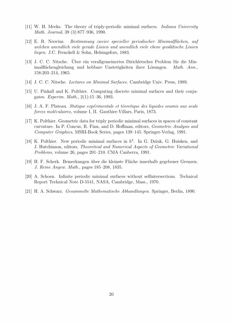
[11] W. H. Meeks. The theory of triply-periodic minimal surfaces. Indiana UniversityMath. Journal, 39 (3):877–936, 1990.
[12] E. R. Neovius. Bestimmung zweier specieller periodischer Minimalflachen, aufwelchen unendlich viele gerade Linien und unendlich viele ebene geodatische Linienliegen. J.C. Frenckell & Sohn, Helsingsfors, 1883.
[13] J. C. C. Nitsche. Uber ein verallgemeinertes Dirichletsches Problem fur die Min-imalflachengleichung und hebbare Unstetigkeiten ihrer Losungen. Math. Ann.,158:203–214, 1965.
[14] J. C. C. Nitsche. Lectures on Minimal Surfaces. Cambridge Univ. Press, 1989.
[15] U. Pinkall and K. Polthier. Computing discrete minimal surfaces and their conju-gates. Experim. Math., 2(1):15–36, 1993.
[16] J. A. F. Plateau. Statique experimentale et teoretique des liquides soumis aux seuleforces moleculaires, volume I, II. Gauthier-Villars, Paris, 1873.
[17] K. Polthier. Geometric data for triply periodic minimal surfaces in spaces of constantcurvature. In P. Concus, R. Finn, and D. Hoffman, editors, Geometric Analysis andComputer Graphics, MSRI-Book Series, pages 139–145. Springer-Verlag, 1991.
[18] K. Polthier. New periodic minimal surfaces in h3. In G. Dziuk, G. Huisken, andJ. Hutchinson, editors, Theoretical and Numerical Aspects of Geometric VariationalProblems, volume 26, pages 201–210. CMA Canberra, 1991.
[19] H. F. Scherk. Bemerkungen uber die kleinste Flache innerhalb gegebener Grenzen.J. Reine Angew. Math., pages 185–208, 1835.
[20] A. Schoen. Infinite periodic minimal surfaces without selfintersections. TechnicalReport Technical Note D-5541, NASA, Cambridge, Mass., 1970.
[21] H. A. Schwarz. Gesammelte Mathematische Abhandlungen. Springer, Berlin, 1890.
20