construction of transition matrices for reversible markov chains
TRANSCRIPT

Construction of Transition Matrices
of Reversible Markov Chains
by
Qian Jiang
A Major Paper
Submitted to the Faculty of Graduate Studies
through the Department of Mathematics and Statistics
in Partial Fulfillment of the Requirements for
the Degree of Master of Science at the
University of Windsor
Windsor, Ontario, Canada
2009
c© 2009 Jiang Qian

Construction of Transition Matrices
of Reversible Markov Chains
by
Qian Jiang
APPROVED BY:
—————————————————————–M. Hlynka
Department of Mathematics and Statistics
—————————————————————–S. Nkurunziza
Department of Mathematics and Statistics
August, 2009

iii
Author’s Declaration of Originality
I hereby certify that I am the sole author of this major paper and that no part of
this major paper has been published or submitted for publication.
I certify that, to the best of my knowledge, my major paper does not infringe upon
anyone’s copyright nor violate any proprietary rights and that any ideas, techniques,
quotations, or any other material from the work of other people included in my
thesis, published or otherwise, are fully acknowledged in accordance with the standard
referencing practices. Furthermore, to the extent that I have included copyrighted
material that surpasses the bounds of fair dealing within the meaning of the Canada
Copyright Act, I certify that I have obtained a written permission from the copyright
owner(s) to include such materials in my major paper and have included copies of
such copyright clearances to my appendix.
I declare that this is a true copy of my major paper, including any final revisions, as
approved by my committee and the Graduate Studies office, and that this major paper
has not been submitted for a higher degree to any other University or Institution.

iv
Abstract
This major paper reviews methods for generating transition matrices of reversible
Markov processes, and introduces several new methods. A method to check for re-
versibility from a given finite state transition matrix is presented through the use of
a computer program in R.

v
Acknowledgments
I would like to express my most profound gratitude to my supervisor, Dr. Hlynka,
whose selfless help, stimulating suggestions and encouragement helped me in all the
time of research for and writing of this major paper. I appreciate him for awarding
me the research funding for this research and for understanding me when I am at the
important point in my life.
Moreover, thanks to Dr. Nkurunziza, as the department reader.
Especially thanks to my unborn baby. Your existence imparts valuable life to me
and the whole family.
My last thanks is to my beloved husband Eric for your endless love.
Contents
Author’s Declaration of Originality iii
Abstract iv
Acknowledgments v
List of figures ix
List of tables x
1 Introduction 1
1.1 Reversible Markov Chains . . . . . . . . . . . . . . . . . . . . . . . . 1
1.2 Technology to check reversibility . . . . . . . . . . . . . . . . . . . . . 3
1.2.1 Calculation of limiting probabilities . . . . . . . . . . . . . . 3
1.2.2 Checking for reversibility . . . . . . . . . . . . . . . . . . . . . 5
2 Kolmogorov’s Criterion and Symmetric Zeros 7
2.1 Kolmogorov’s Criterion . . . . . . . . . . . . . . . . . . . . . . . . . . 7
2.2 Number of checks required. . . . . . . . . . . . . . . . . . . . . . . . . 9
2.3 Nonsymmetric zero entries . . . . . . . . . . . . . . . . . . . . . . . . 12
3 Metropolis-Hastings Algorithm 13
vi

CONTENTS vii
3.1 Discussion and Algorithm . . . . . . . . . . . . . . . . . . . . . . . . 13
3.2 Main Property . . . . . . . . . . . . . . . . . . . . . . . . . . . . . . 14
4 Simple Reversible Matrices 17
4.1 Symmetric transition matrices . . . . . . . . . . . . . . . . . . . . . . 17
4.2 Equal row entries (except diagonal) . . . . . . . . . . . . . . . . . . . 18
4.3 Equal column entries (except diagonal) . . . . . . . . . . . . . . . . . 19
4.4 Reversible Birth-Death and Quasi-Birth-Death Process(QBD) . . . . 20
5 Scaling of Transition Rates 23
5.1 Scale symmetric pairs . . . . . . . . . . . . . . . . . . . . . . . . . . . 23
5.2 Scale rows or columns except diagonal . . . . . . . . . . . . . . . . . 25
6 Product: symmetric and diagonal matrices 30
6.1 Product of symmetric and diagonal matrices . . . . . . . . . . . . . . 30
7 Graph Method 36
7.1 Graph Method . . . . . . . . . . . . . . . . . . . . . . . . . . . . . . 36
8 Tree Process 39
8.1 Definition . . . . . . . . . . . . . . . . . . . . . . . . . . . . . . . . . 39
8.2 Example . . . . . . . . . . . . . . . . . . . . . . . . . . . . . . . . . . 40
9 Triangular completion method 43
9.1 Algorithm . . . . . . . . . . . . . . . . . . . . . . . . . . . . . . . . . 43
9.2 Example . . . . . . . . . . . . . . . . . . . . . . . . . . . . . . . . . . 44
10 Convex Combination 47
10.1 Weighted Average . . . . . . . . . . . . . . . . . . . . . . . . . . . . . 47

CONTENTS viii
10.2 Example . . . . . . . . . . . . . . . . . . . . . . . . . . . . . . . . . . 48
11 Reversibility and Invariance 50
11.1 P+P∗2
. . . . . . . . . . . . . . . . . . . . . . . . . . . . . . . . . . . 50
11.2 P ∗P . . . . . . . . . . . . . . . . . . . . . . . . . . . . . . . . . . . . 53
12 Expand and Merge Methods 55
12.1 State by State Expand . . . . . . . . . . . . . . . . . . . . . . . . . . 55
12.2 Merge Method . . . . . . . . . . . . . . . . . . . . . . . . . . . . . . . 57
13 Summary 62
Bibliography 62

List of Figures
1.1 Computing limiting probabilities with R . . . . . . . . . . . . . . . . 5
1.2 Checking symmetry with R . . . . . . . . . . . . . . . . . . . . . . . 5
7.1 Graph with nodes . . . . . . . . . . . . . . . . . . . . . . . . . . . . . 37
8.1 Tree structure . . . . . . . . . . . . . . . . . . . . . . . . . . . . . . . 40
8.2 Tree structure example . . . . . . . . . . . . . . . . . . . . . . . . . . 41
12.1 Process A . . . . . . . . . . . . . . . . . . . . . . . . . . . . . . . . 57
12.2 Process B . . . . . . . . . . . . . . . . . . . . . . . . . . . . . . . . 58
12.3 Merged graph . . . . . . . . . . . . . . . . . . . . . . . . . . . . . . 59
ix

List of Tables
2.1 Sequence of checking . . . . . . . . . . . . . . . . . . . . . . . . . . . 11
x

Chapter 1
Introduction
1.1 Reversible Markov Chains
According to Ross, a stochastic process {Xn, n = 0, 1, 2, . . . } such that
P{Xn+1 = j|Xn = i, Xn−1 = in−1, . . . , X1 = i1, X0 = i0} = P{Xn+1 = j|Xn = i}
is a Markov chain.
Some books that discuss reversibility include Aldous and Fill (2002), Kelly (1979),
Nelson (1995), Kao (1997), and Wolff (1989). Other books will be mentioned as they
are referred to in this major paper.
According to Strook (2005), a class of Markov processes is said to be reversible
if, on every time interval, the distribution of the process is the same when it is run
backward as when it is run forward. That is, for any n ≥ 0 and (i0, · · · , in) ∈ S(n+1),
in the discrete time setting,
P (Xm = im for 0 ≤ m ≤ n) = P (X(n−m) = im for 0 ≤ m ≤ n) (1.1)
and in the continuous time setting,
P (X(tm) = im for 0 ≤ m ≤ n) = P (X(tn − tm) = im for 0 ≤ m ≤ n) (1.2)
1
CHAPTER 1. INTRODUCTION 2
whenever 0 = t0 ≤ · · · ≤ tn. Indeed, depending on whether the setting is that of
discrete or continuous time, we have
P (X0 = i, Xn = j) = P (X0 = j, Xn = i)
or
P (X(0) = i, X(t) = j) = P (X(t) = i, X(0) = j)
In fact, reversibility says that, depending on the setting, the joint distribution of
(X0, Xn) (or (X(0), X(t))) is the same as that of (Xn, X0) (or (X(t), X(0))).
If P is the transition probability matrix, then , by taking n = 1 in equation (1.1),
we see that
πipij = P (X0 = i ∩ X1 = j) = P (X0 = j ∩ X1 = i) = πjpji.
That is, P satisfies
πipij = πjpji, the condition of detailed balance. (1.3)
Conversely, (1.3) implies reversibility. To see this, one works by induction on
n ≥ 1 to check that
πi0pi0i1 · · · pin−1in = πinpinin−1 · · · pi1i0,
which is equivalent to (1.1). Further, we can verify that a reversible process is
stationary since it has the invariant distributions.
We summarize the above discussion in the form of a theorem.
The following statement is from Rubinstein and Kroese (2007).
Theorem 1.1.1.
A stationary process is reversible if and only if there exists a positive collection of
numbers {πi} summing to unity such that
πipij = πjpji for all i, j ∈ S

CHAPTER 1. INTRODUCTION 3
Whenever such a collection exists, it is the equilibrium distribution.
According to Rubinstein (2007): “Intuitively, πipij can be thought of as the prob-
ability flux from state i to state j. Thus the detailed balance equations say that the
probability flux from state i to state j equals that from state j to state i.” This inter-
pretation is helpful for constructing transition matrices of reversible Markov chains.
1.2 Technology to check reversibility
The detailed balance equation allows us to determine if a process is reversible based
on the transition probability matrix and the limiting probabilities. We designed a
method to check the reversibility of a Markov chain based on the detailed balance
equations. Specifically, we use an R program (R 2.9.0) to help compute the limiting
probabilities and related calculations.
Henceforth, when we mention reversible matrix or a matrix which is reversible, we
actually mean the transition matrix of a reversible Markov process. This terminology
is used for conciseness.
1.2.1 Calculation of limiting probabilities
Let P be the transition matrix of a Markov chain. Let P (n) be the n step transition
matrix. Let P n be the n-th power of the transition matrix. Let Π = limn→∞ P n, if
the limit exists. Let π be the limiting probability vector, if it exists.
Then we know that
Π = limn→∞
P (n) = limn→∞
P n
and each common row of Π, is π, the limiting vector.
CHAPTER 1. INTRODUCTION 4
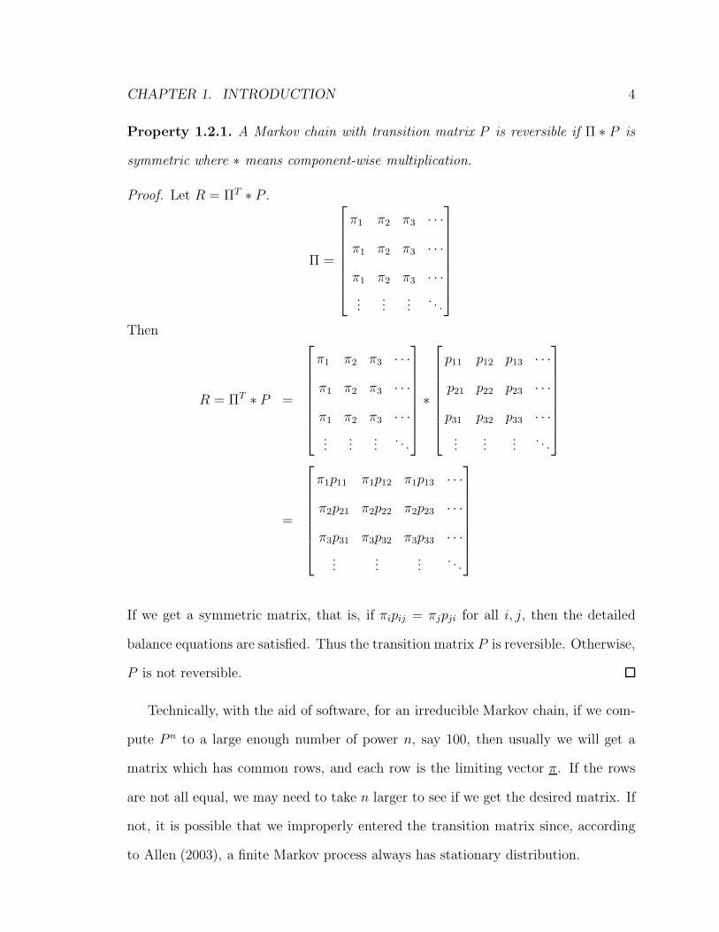
Property 1.2.1. A Markov chain with transition matrix P is reversible if Π ∗ P is
symmetric where ∗ means component-wise multiplication.
Proof. Let R = ΠT ∗ P .
Π =
π1 π2 π3 · · ·π1 π2 π3 · · ·π1 π2 π3 · · ·...
......
. . .
Then
R = ΠT ∗ P =
π1 π2 π3 · · ·π1 π2 π3 · · ·π1 π2 π3 · · ·...
......
. . .
∗
p11 p12 p13 · · ·p21 p22 p23 · · ·p31 p32 p33 · · ·...
......
. . .
=
π1p11 π1p12 π1p13 · · ·π2p21 π2p22 π2p23 · · ·π3p31 π3p32 π3p33 · · ·
......
.... . .
If we get a symmetric matrix, that is, if πipij = πjpji for all i, j, then the detailed
balance equations are satisfied. Thus the transition matrix P is reversible. Otherwise,
P is not reversible.
Technically, with the aid of software, for an irreducible Markov chain, if we com-
pute P n to a large enough number of power n, say 100, then usually we will get a
matrix which has common rows, and each row is the limiting vector π. If the rows
are not all equal, we may need to take n larger to see if we get the desired matrix. If
not, it is possible that we improperly entered the transition matrix since, according
to Allen (2003), a finite Markov process always has stationary distribution.

CHAPTER 1. INTRODUCTION 5
1.2.2 Checking for reversibility
Consider as an example the transition matrix P =
.5 .25 .25
.5 0 .5
.25 .25 .5
.
In R, we apply the commands as in Figure 1.1
Figure 1.1: Computing limiting probabilities with R
As we see, the limiting vector of P is π = (0.4, 0.2, 0.4). We transpose P 100 and
compute (P 100)T ∗ P .
In R, we compute this procedure as in Figure 1.2 (continued from Figure 1.1)
Figure 1.2: Checking symmetry with R
In this example, we get a symmetric matrix, and conclude that P is reversible.

CHAPTER 1. INTRODUCTION 6
So far, we have given a method to check the reversibility of a transition matrix
with aid of an R program. In the later discussion of ways to construct reversible
matrices, we will always use this method to test the validity of the examples.
For the remainder of this paper, we will assume that our Markov chains are all
irreducible, aperiodic, and positive recurrent. Thus the limiting vector will always
exist, be nonzero, and not depend on the initial state.
Although we will be dealing mainly with reversibility in discrete time Markov
chains and probability transition matrices, most of the results hold for continuous
time Markov processes and rate matrices (infinitesimal generators).

Chapter 2
Kolmogorov’s Criterion and
Symmetric Zeros
2.1 Kolmogorov’s Criterion
Kolmogorov’s Criterion is a method to check and the reversibility of a transition
matrix, without requiring knowledge of the limiting probability vector. It can also be
used as a method to construct transition matrices of reversible Markov process and
to validate some of the other methods in this paper.
The following is taken from Ross (2002). It is included here since the result is
used frequently in this paper.
Theorem 2.1.1. (Kolmogorov Criterion) A stationary Markov chain is reversible if
and only if, any path starting from state i and back to i has the same probability as
the path going in the reverse direction. That is, the chain is reversible iff
pii1pi1i2 · · · piki = piikpikik−1· · · pi1i (2.1)
∀k and i, i1, i2, · · · , ik ∈ S.
7

CHAPTER 2. KOLMOGOROV’S CRITERION AND SYMMETRIC ZEROS 8
Proof. We prove the necessity first.
If a Markov chain is reversible, the detailed balance equations are
πipii1 = πi1pi1i
πi1pi1i2 = πi2pi2i1
...
πik−1pik−1ik = πikpikik−1
πikpiki = πipiik
∀k and i, i1, i2, · · · , ik ∈ S.
Multiply both sides of the reversibility equations together, and cancel out the common
part πiπi1 · · ·πik to get
pii1pi1i2 · · · piki = piikpikik−1· · · pi1i.
∀k and i, i1, i2, · · · , ik ∈ S.
Next we prove sufficiency.
Fix states i and j and rewrite Equation (2.1) as
pii1pi1i2 · · · pikjpji = pijpjikpikik−1· · · pi1i (2.2)
Now pii1pi1i2 · · · pikj is the probability of starting from state i, moving to state j
after k steps and then going into state i at (k + 1)th step. Similarly pjikpikik−1· · · pi1i
is the probability of starting from state j, moving to state i after k steps and then
moving into state j at (k + 1)th step. Hence, summing both sides of Equation (2.2)
over all intermediate states i1, i2, · · · , ik yields
pk+1ij pji = pijp
k+1ji

CHAPTER 2. KOLMOGOROV’S CRITERION AND SYMMETRIC ZEROS 9
Summing over k shows that
pji
∑nk=1 pk
ij
n= pij
∑nk=1 pk
ji
n
Letting n → ∞ yields
πjpji = πipij
thus showing that the chain is reversible.
Knowing this powerful condition, we can construct transition matrices of Markov
chain by making the probability of one path equal to the probability of its reversed
path. However, Kolmogorov’s condition is mainly used for reversibility verification
and proof.
Example 2.1.1.
I simply give a 3 × 3 transition matrix for example.
P =
.2 .4 .4
.3 .4 .3
.5 .5 0
Thus p12p23p31 = (.4)(.3)(.5) = p13p32p21 = (.4)(.5)(.3)
For a 3× 3 transition matrix, it turns out that only one detailed balance equation has
to be checked. So P is reversible.
2.2 Number of checks required.
We believe that the following result is new.
Property 2.2.1. For an n×n transition matrix, the number of distinct Kolmogorov
equations that must be checked is
n∑i=3
(n
i
)(i − 1)!
2.

CHAPTER 2. KOLMOGOROV’S CRITERION AND SYMMETRIC ZEROS 10
Proof. We note that using Kolmogorov’s condition to check a 2× 2 transition matrix
means checking that p12p21 = p21p12. For a two-state matrix, we even do not need
to check at all because the probabilities always satisfy Kolmogorov’s condition, i.e.,
a two-state transition matrix is always reversible. Then we are led to ask that how
many equations need to be checked for larger state space matrices.
We note that using Kolmogorov’s condition to check a 3× 3 matrix is very simple
because the number of equations to be checked is only one. One finds that all the
different paths of Kolmogorov’s condition reduce to a single equation.
For a 4×4 transition matrix, we must check all three state paths and all four state
paths. As to the three state paths, we choose any three states out of four and for each
three-state path, we check only once, while for the four-state paths, we can assume
that starting state is fixed. Then there are 3! paths for the other states. However,
since the other side of equation is just the reversed path, we are reduced to 3!2
paths
involving four states. In total, we need to check((43) + 3!
2= 7
)equations.
Similarly for a 5 × 5 transition matrix, we must check all the three-state paths,
four-state paths and five-state paths, that is((53) + (5
4)(4−1)!
2+ (5−1)!
2
)= 37 equations
to ensure the validity of Kolmogorov’s condition.
The same argument works for any n × n transition matrix.
The following Table 2.1 shows this relation clearly.
This gives an interesting sequence as shown in the right column of the table.
The sequence was checked at The On-Line Encyclopedia of Integer Sequences, a
web site on integer sequences. For anyone who is interested, please see
http://www.research.att.com/∼njas/sequences/Seis.html
The sequence already existed there but had only one explanation. A second expla-
nation was therefore added to note that it gives the number of Kolmogorov type

CHAPTER 2. KOLMOGOROV’S CRITERION AND SYMMETRIC ZEROS 11
Numberofstates Numberofchecking
0 0
1 0
2 0
3 1
4 7
5 37
6 197
7 1172
8 8018
9 62814
10 556014
Table 2.1: Sequence of checking
equations that must be checked for reversibility. The note appears on the web site as
follows.
A002807 Sum {k=3..n} (k-1)!*C(n,k)/2.
(Formerly M4420 N1867)
0, 0, 0, 1, 7, 37, 197, 1172, 8018, 62814, 556014, 5488059, 59740609, 710771275,
9174170011, 127661752406, 1904975488436, 30341995265036, 513771331467372,
9215499383109573, 174548332364311563, 3481204991988351553,
72920994844093191553, 160059637159039967178
COMMENT Maximal number of cycles in complete graph on n nodes.
- Erich Friedman (erich.friedman(AT)stetson.edu).
Number of equations that must be checked to verify reversibility of
an n state Markov chain using the Kolmogorov criterion

CHAPTER 2. KOLMOGOROV’S CRITERION AND SYMMETRIC ZEROS 12
- From Qian Jiang (jiang1h(AT)uwindsor.ca), Jun 08 2009
2.3 Nonsymmetric zero entries
Another useful result is the following.
Theorem 2.3.1.
A transition matrix is not reversible if there exists any nonsymmetric zero entry
in the matrix.
Proof.
The proof is quite simple because either the detailed balance equation or the
Kolmogorov’s condition is violated in such cases.
Example 2.3.1.
Consider the transition matrix
P =
.5 .3 .1 .1
.4 .2 .1 .3
.1 0 .7 .2
.2 .1 .3 .4
We do not need to bother the checking method in Chapter 1 and we are sure that
P is not reversible since there is a 0 entry in the (3,2) position which has a non-zero
in the (2,3) position.
Chapter 3
Metropolis-Hastings Algorithm
3.1 Discussion and Algorithm
According to Rubinstein (2007) “The main idea behind the Metropolis-Hastings al-
gorithm is to simulate a Markov chain such that the stationary distribution of this
chain coincides with the target distribution.”
Such a problem arises naturally: Given a probability distribution {πi} on a state
space S, how can we construct a Markov chain on S that has {πi} as a stationary
distribution, and prove that such a Markov chain is reversible with respect to {πi}?According to Evans and Rosenthal (2004), given Xn = i, the Metropolis-Hastings
algorithm computes the value Xn+1 as follows.
• We are given π. Pick any Markov chain [qij] transition matrix with size given
by the number of states.
• Choose Yn+1 = j according to the Markov chain {qij}.
• Set αij = min{
1,πjqji
πiqij
}(the acceptance probability)
13

CHAPTER 3. METROPOLIS-HASTINGS ALGORITHM 14
• With probability αij, let Xn+1 = Yn+1 = j (i.e.,accepting the proposal Yn+1).
Otherwise, with probability 1 − αij , let Xn+1 = Xn = i (i.e. rejecting the
proposal Yn+1).
3.2 Main Property
Property 3.2.1. The Metropolis-Hastings algorithm results in a Markov chain
X0, X1, X2, · · · , which has {πi} as a stationary distribution, and the resulting Markov
chain is reversible with respect to {πi}, i.e.,
πiP (Xn+1 = j|Xn = i) = πjP (Xn+1 = i|Xn = j),
for i, j ∈ S.
Proof. (Evans and Rosenthal)
We will prove the reversibility of the Markov chain first, and then show that such
{πi} is the stationary distribution for the chain.
πiP (Xn+1 = j|Xn = i) = πjP (Xn+1 = i|Xn = j), is naturally true if i = j, so we
will assume that i �= j.
But if i �= j, and Xn = i, then the only way we can have Xn+1 = j is if Yn+1 =
j(i.e., we propose the state j, which we will do with probability pij).Also we accept
this proposal (which we will do with probability αij . Hence
P (Xn+1 = j|Xn = i) = qijαij = qijmin
{1,
πjqji
πiqij
}= min
{qij,
πjqji
πi
}.
It follows that πiP (Xn+1 = j|Xn = i) = min{πiqij, πjqji}.Similarly, we compute that πjP (Xn+1 = i|Xn = j) = min{πjqji, πiqij} .
It follows that πiP (Xn+1 = j|Xn = i) = πjP (Xn+1 = i|Xn = j) is true for all
i, j ∈ S, i.e., the Markov chain made from the Metropolis-Hastings algorithm is a
reversible chain with respect to {πi}.

CHAPTER 3. METROPOLIS-HASTINGS ALGORITHM 15
Now we shall prove that if a Markov chain is reversible with respect to {πi}, then
{πi} is a stationary distribution for the chain.
We compute, using reversibility, that for any j ∈ S,
∑i∈S
πipij =∑i∈S
πjpji = πj
∑i∈S
pji = πj(1) = πj.
Hence, {πi} is a stationary distribution.
Example 3.2.1. We have not found any book which give matrix type examples. We
present one such example here.
Step 1. Given an arbitrary π
π = (.1, .2, .3, .4)
Step 2. Make up a Markov chain {Yi} which has transition matrix Q (a simple
one).
Q =
.2 .2 .3 .3
.2 .2 .3 .3
.1 .1 .5 .3
.4 .2 .1 .3
Step 3. Calculate αij, leaving the diagonal empty.
α12 = min
{1,
π2q21
π1q12
}= min
{1,
.2(.2)
.1(.2)
}= 1
Similarly, we compute out all the {αij} and get matrix α
α =
1 1 1
12
12
1
1 1 49
316
34
1

CHAPTER 3. METROPOLIS-HASTINGS ALGORITHM 16
Step 4. Multiply Q and α (here we use the element by element multiplication, not
the matrix product). Then fill in the diagonals so the rows sum to one and get a new
transition matrix P .
P =
.2 .2 .3 .3
.1 .45 .15 .3
.1 .1 23
215
340
320
.1 2740
Now we are to check the reversible nature of P using R as in Section 1.2.2.
P 100 =
0.1 0.2 0.3 0.4
0.1 0.2 0.3 0.4
0.1 0.2 0.3 0.4
0.1 0.2 0.3 0.4
,
which means the limiting vector is π = [0.1, 0.2, 0.3, 0.4]. It is identical to the limiting
vector we start with.
Also
(P 100)T ∗ P =
0.02 0.02 0.03 0.03
0.02 0.09 0.03 0.06
0.03 0.03 0.20 0.04
0.03 0.06 0.04 0.27
,
is a symmetric matrix and that verifies the reversibility of P.
Chapter 4
Simple Reversible Matrices
4.1 Symmetric transition matrices
The following result is well known. See Kijima (1997), for example.
Property 4.1.1. Markov chains defined by symmetric transition matrices are always
reversible, i.e.,
pijπi = pjiπj
is always true for all i, j ∈ S.
Proof.
Suppose that a transition matrix itself is symmetric, i.e. pij = pji for all i and j.
Then, since∑
j pij =∑
j pji = 1, the transition matrix is doubly stochastic, i.e. a
square matrix of nonnegative real numbers, each of whose rows and columns sums to
1. The stationary distribution of a finite, doubly stochastic matrix is uniform (omit
proof here). Specifically, πi = 1n, where n is the number of states.
Hence, pijπi = pjiπj holds for all i, j ∈ S, the corresponding Markov chain is
reversible.
17

CHAPTER 4. SIMPLE REVERSIBLE MATRICES 18
Example 4.1.1. Given a 4 ∗ 4 symmetric transition matrix P
P =
.3 .2 .1 .4
.2 .5 0 .3
.1 0 .7 .2
.4 .3 .2 .1
The uniform stationary distribution π1 = π2 = π3 = π4 = .25, thus the reversibility
follows.
4.2 Equal row entries (except diagonal)
We believe the following result is new (as we have not found it in the literature).
Property 4.2.1. A transition matrix which has equal entries within each row, except
perhaps the diagonal entry, is reversible.
Proof. Consider a transition matrix with states {S}, with equal row entries, except
perhaps the diagonal ones. A path from state i back to state i has probability
pijpjk . . . plmpmi (4.1)
∀i, j, · · · , l, m ∈ S.
Here we are always supposed to transit from one state to different state in one
step, i.e., we are not stuck at any state (so the diagonal entries need not equal the
other row entries), which is consistent with Kolmogorov’s condition.
If we reverse this path, it will be
pimpml · · · pkjpji (4.2)

CHAPTER 4. SIMPLE REVERSIBLE MATRICES 19
∀i, j, · · · , l, m ∈ S
Since the row entries are equal, we can match every entry in (4.1) with an entry
in (4.2), by simply finding the same row subscript.
Therefore (4.1)=(4.2) for any number of steps of the path, which clearly satisfies
Kolmogorov’s criterion. We conclude that a Markov transition matrix with equal row
entries (except possibly the diagonal entries) is reversible.
Example 4.2.1. We make up a transition matrix P which has equal row entries,
P =
.5 .25 .25
.3 .4 .3
.125 .125 .75
We check its reversibility using R and get the limiting vector is
π = (0.2608696, 0.2173913, 0.5217391)
and
(P 100)T ∗ P =
0.13043478 0.06521739 0.06521739
0.06521739 0.08695652 0.06521739
0.06521739 0.06521739 0.39130435
.
P is verified to be reversible.
4.3 Equal column entries (except diagonal)
We believe the following result is new.
Property 4.3.1. A transition matrix which has equal entries within each column,
except possibly the diagonal entry, is reversible.
Proof. The proof is similar to the proof for rows.

CHAPTER 4. SIMPLE REVERSIBLE MATRICES 20
Example 4.3.1.
P =
.3 .4 .3
.25 .45 .3
.25 .4 .35
.
We can conclude its reversibility since the entries within each column (except the
diagonal) are all equal.
Another interesting example in this category worth mentioning is
P =
12
14
18
· · ·12
14
18
· · ·12
14
18
· · ·...
......
...
,
which has equal entries in each column, identical rows and each row is an infinite
sequence. Such a matrix obviously has as its limiting vector any row of the matrix
so if we wish to find a matrix with a given π, we can construct such a matrix by
taking the rows all equal to π. This is the only infinite state transition matrix which
appears in this paper. This matrix is reversible since all the columns have equal
entries. We can then modify this matrix, using our methods, to create many other
reversible transition matrices.
4.4 Reversible Birth-Death and Quasi-Birth-Death
Process(QBD)
According to Kelly (1979), any birth-death process is reversible iff the detailed balance
equation is satisfied. We omit the proof here. For the general proof, see Kelly(1979).
Thus, consider a birth-death process which has common birth probability λ and
common death probability µ, and the transition matrix

CHAPTER 4. SIMPLE REVERSIBLE MATRICES 21
P =
−λ λ 0 0 · · ·µ −(µ + λ) λ 0 · · ·0 µ −(µ + λ) λ · · ·0 0 µ −(µ + λ) · · ·...
......
......
(4.3)
The local balance equation πi(λi + µi) = πi+1µi+1 + πi−1µi−1 is always satisfied thus
the Markov process is reversible.
Then we consider a simple quasi birth-death process with two levels of states
which defined by transition matrix
Q =
∗ λ a 0 0 · · ·µ ∗ λ a 0 · · ·b µ ∗ λ a · · ·0 b µ ∗ λ · · ·...
......
......
...
(4.4)
where we use (*) in the place of diagonal entries to make the matrix look clear.
This is a quasi birth-death process of the form
Q =
A1 A0 0 0 . . .
A2 A1 A0 0 . . .
0 A2 A1 A0 . . .
0 0 A2 A1 . . .
......
......
. . .
, (4.5)
where A0 =
a 0
λ a
, A1 =
∗ λ
µ ∗
, A2 =
b µ
0 b
.
This model would be appropriate for a queueing system which allows arrivals of
single or paired customers and allows service of single or paired customers.

CHAPTER 4. SIMPLE REVERSIBLE MATRICES 22
Usually, to find the solution of stationary distribution of QBD process is not very
easy. See Nelson (1995, Chapter 9) and Jain (2006, Chapter 8). However, if the QBD
is reversible, then to work out the stationary distribution πi would be quite simple
by using the detailed balance equation and the fact that∑
i πi = 1.
Here we are interested in finding a and b such that Q is reversible. Again from
the detailed balance equations, if Q is reversible, then
πi+1
πi=
pi,i+1
pi+1,i=
λ
µ,
that is, Q has the same stationary distribution as that of P. Also we get
a
b=
pi,i+2
pi+2,i=
πi+2
πi=
πi+2
πi+1
πi+1
πi= (
λ
µ)2.
In summary, we state the above discussion as a property, which we believe to be
new.
Property 4.4.1. For a Quasi-Birth-Death process which is defined by transition ma-
trix Q, where Q has λ, µ as the first level transition probabilities and a, b as the second
ones (just as shown in equation 4.4), if ab
= (λµ)2, then Q is the transition matrix of
a reversible Quasi-Birth-Death process.
This result can be valuable to check the validity and accuracy of iterative methods
for solving QBD’s.
Chapter 5
Scaling of Transition Rates
5.1 Scale symmetric pairs
According to Nelson (1995), we introduce the following method.
Property 5.1.1. By changing the symmetric pairs of a reversible transition matrix
P by the same proportion, then adjusting the diagonal entries to make rows sum to
1, if possible, we get a new reversible transition matrix which has the same limiting
probabilities as the original one.
i.e. Let p′i0j0= api0j0 and p′j0i0
= apj0i0 for fixed i0, j0 ∈ S, and leave all other pij
alone.
If the resulting matrix is P ′, then P ′ is reversible as well with the same limiting
probability vector as P .
Proof. Consider a reversible Markov process {X}, and then a new process {X ′} can
be obtained from X by modifying the transition rates between states i0 and j0 in
symmetric pairs by a multiplicative factor
p′i0j0= api0j0 and p′j0i0
= apj0i0
23
CHAPTER 5. SCALING OF TRANSITION RATES 24
Actually, we can do the symmetric modification as many times as one likes.
Kolmogorov’s criterion implies that {X ′} is also reversible, since the all the path
probability equations involving both i0 and j0 are changed in by exactly the same
factor and hence still hold.
Further, the ratios of stationary distribution of {X ′} are exactly the same as those
of {X},since π′
i0p′i0j0
= π′j0
p′j0i0
impliesπ′
i0
π′j0
=p′j0i0
p′i0j0
=apji
apij
=pji
pij
=πi
πj
,
which implies that the stationary distribution of {X ′} is identical to that of {X}.
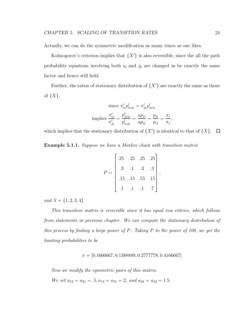
Example 5.1.1. Suppose we have a Markov chain with transition matrix
P =
.25 .25 .25 .25
.3 .1 .3 .3
.15 .15 .55 .15
.1 .1 .1 .7
,
and S = {1, 2, 3, 4}This transition matrix is reversible since it has equal row entries, which follows
from statements in previous chapter. We can compute the stationary distribution of
this process by finding a large power of P . Taking P to the power of 100, we get the
limiting probabilities to be
π = [0.1666667, 0.1388889, 0.2777778, 0.4166667]
Now we modify the symmetric pairs of this matrix.
We set a12 = a21 = .5, a13 = a31 = 2, and a24 = a42 = 1.5.
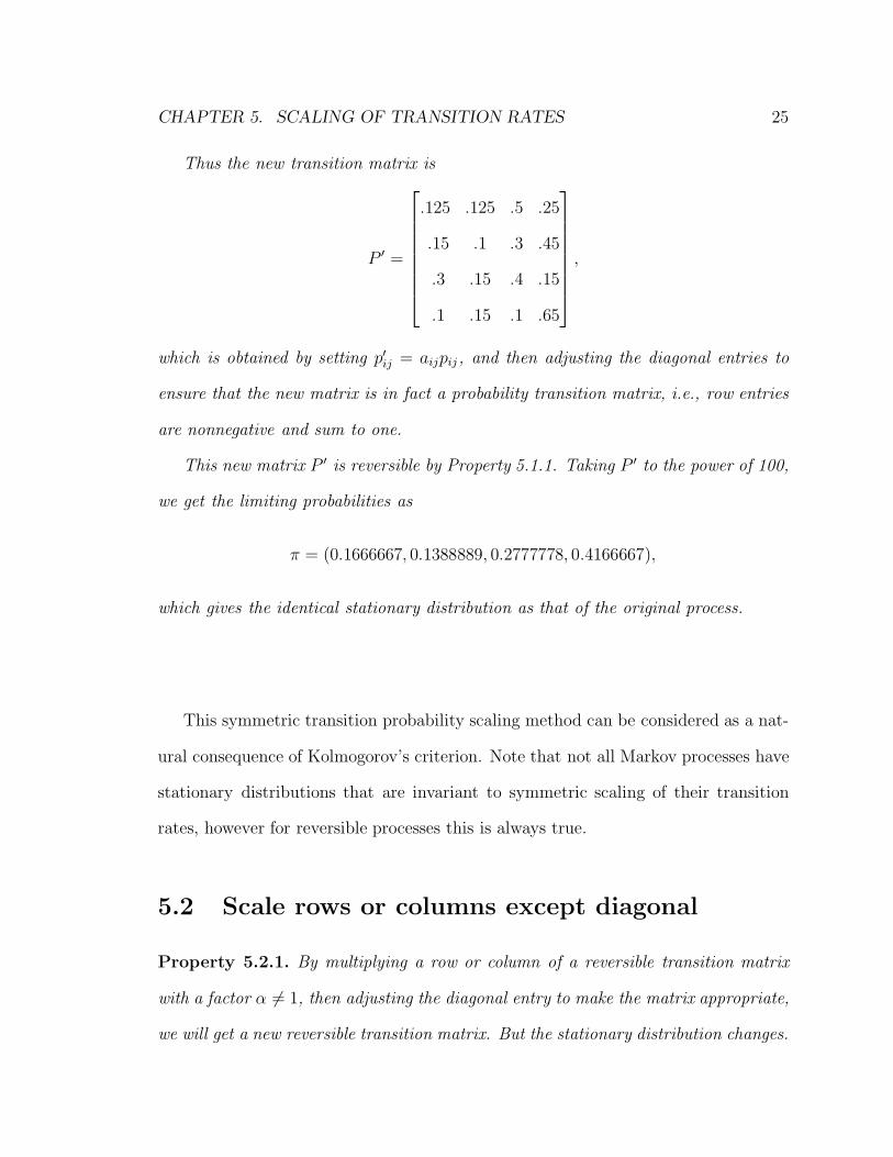
CHAPTER 5. SCALING OF TRANSITION RATES 25
Thus the new transition matrix is
P ′ =
.125 .125 .5 .25
.15 .1 .3 .45
.3 .15 .4 .15
.1 .15 .1 .65
,
which is obtained by setting p′ij = aijpij , and then adjusting the diagonal entries to
ensure that the new matrix is in fact a probability transition matrix, i.e., row entries
are nonnegative and sum to one.
This new matrix P ′ is reversible by Property 5.1.1. Taking P ′ to the power of 100,
we get the limiting probabilities as
π = (0.1666667, 0.1388889, 0.2777778, 0.4166667),
which gives the identical stationary distribution as that of the original process.
This symmetric transition probability scaling method can be considered as a nat-
ural consequence of Kolmogorov’s criterion. Note that not all Markov processes have
stationary distributions that are invariant to symmetric scaling of their transition
rates, however for reversible processes this is always true.
5.2 Scale rows or columns except diagonal
Property 5.2.1. By multiplying a row or column of a reversible transition matrix
with a factor α �= 1, then adjusting the diagonal entry to make the matrix appropriate,
we will get a new reversible transition matrix. But the stationary distribution changes.

CHAPTER 5. SCALING OF TRANSITION RATES 26
Proof. :
Consider a reversible Markov chain, with state space S, which is defined by transition
matrix P . If we change the i-th row from pij to p′ij = αpij for all j ∈ S, then any
equation of Kolmogorov’s criterion involving state i for the new matrix P ′ looks like
· · · pkip′ijpjl · · · = · · · pljpjip
′ik · · ·
⇔ · · · pkiαpijpjl · · · = · · · pljpjiαpik · · ·
⇔ · · · pkipijpjl · · · = · · · pljpjipik · · ·
which is true by the Kolmogorov Criterion since the original transition matrix P is
reversible.
Example 5.2.1. : Consider the transition matrix
P =
.45 .3 .15 .1
.25 .5 .15 .1
.25 .3 .35 .1
.25 .3 .15 .3
,
which is reversible by Property (4.3.1) since it has equal column entries except the
diagonal. We compute its limiting probabilities and get
π = (0.3125, 0.315, 0.1875, 0.125).
We modify this matrix by multiplying the row with a constant factor bi with respect
to ith row, and then adjust the diagonal entries to make the new transition matrix
proper.
For instance we set b1 = 1.5, b2 = 1.2, b3 = .8 and b4 = 1, and adjust the diagonal

CHAPTER 5. SCALING OF TRANSITION RATES 27
entries. We get a new transition matrix
P ′ =
.175 .45 .225 .15
.3 .4 .18 .12
.2 .24 .48 .08
.25 .3 .15 .3
.
We compute the limiting probabilities of P ′ and get
π′ = (0.2366864, 0.3550296, 0.2662722, 0.1420118).
Compared to the first scaling method which remains invariant limiting proba-
bilities, this second scaling method has different limiting probabilities after scaling.
We are interested in how the limiting probabilities change. That is expresses in the
following result which is new.
Property 5.2.2. Let P be the transition matrix for reversible Markov Chain with n
states and limiting probability vector π = (π1, . . . , πi, . . . , πn). Modify P by multiplying
row i by m and adjusting the diagonal such that the new matrix P ′ is still a transition
matrix. Then the limiting vector of P ′ is
π′ = (π′1, . . . , π
′i, . . . , π
′n)
= (aπ1, . . . , bπi, . . . , aπn)
where a =m
m + πi(1 − m)and b =
1
m + πi(1 − m).
Proof. In the following, we assume that denominators are never zero and i �= 1. If
these assumptions are not satisfied, then the argument can be adjusted.
By Property 5.2.1, P ′ is reversible. By the detailed balance equations, we have
π′i
π′1
=p′1i
p′i1=
p1i
mpi1= (
1
m)p1i
pi1= (
1
m)πi
π1
CHAPTER 5. SCALING OF TRANSITION RATES 28
Multiplying just row i by a constant will not change the ratios of the other limiting
probabilities so
π′ = (π′1, . . . , π
′i, . . . , π
′n)
= (aπ1, . . . , bπi, . . . , aπn)
and since the probabilities sum to 1, we have
1 = (a(π1 + · · · + πn − πi) + bπi) = a(1 − πi) + bπi. Thus a =1 − bπi
1 − πi. Thus
π′ = (1 − bπi
1 − πiπ1, . . . , bπi, . . . ,
1 − bπi
1 − πiπn).
Hence
π′i
π′1
=bπi(
1 − biπi
1 − πi
)π1
=b(1 − πi)
1 − bπi
πi
π1so
1
m=
b(1 − πi)
1 − bπi.
Solving for b and a gives b =1
m + πi(1 − m)and a =
m
m + πi(1 −m).
To check the result, consider the following example.
Example 5.2.2.
Compose a reversible matrix
P =
.4 .2 .4
.45 .1 .45
.2 .1 .7
P is reversible since it was composed initially from an equal row matrix with a one
time symmetric pair scaling.
The limiting vector of P is
π = [0.2903226, 0.1290323, 0.5806452]

CHAPTER 5. SCALING OF TRANSITION RATES 29
We conduct a row scaling to the second row of P from .45 to .4 (i.e. take m = 8/9)
and then adjust the diagonal entry from p22 = .1 to p∗22 = .2. According to Property
5.2.2, the new limiting probability of state 2 should be
π′2 = bπ2 = 1
m+π2(1−m)π2 =
.1290323
8/9 + 1290323(1 − 8/9)
= 0.1428571
By computing in R, the limiting vector of P ∗ is
π∗ = [0.2857143, 0.1428571, 0.5714286]
which is consistent with the result.

Chapter 6
Product: symmetric and diagonal
matrices
6.1 Product of symmetric and diagonal matrices
The following is taken from Kelly (1979). He does not present a proof and we provide
one here.
Property 6.1.1. A stationary Markov chain is reversible if and only if the matrix
of transition probabilities can be written as the product of a symmetric and a diagonal
matrix. i.e. P is the transition matrix for a reversible Markov chain iff P = SD
where S is a symmetric matrix and D a diagonal matrix such that∑
j pij = 1, ∀k.
Proof.
Part I: We show the necessity first. i.e. Let P = SD where S is a symmetric matrix
and D a diagonal matrix, be such that∑
j pij = 1, ∀k. We will show that P is a
reversible transition matrix.
30

CHAPTER 6. PRODUCT: SYMMETRIC AND DIAGONAL MATRICES 31
Let P = SD =
s11 s12 s13 · · ·s21 s22 s23 · · ·s31 s32 s33 · · ·· · · · · · · · · · · ·
d11 0 0 · · ·0 d22 0 · · ·0 0 d33 · · ·· · · · · · · · · · · ·
=
s11d11 s12d22 s13d33 · · ·s21d11 s22d22 s23d33 · · ·s31d11 s32d22 s33d33 · · ·· · · · · · · · · · · ·
.
Then
(d11, d22, d33, · · · )P
= (d11, d22, d33, · · · )
s11d11 s12d22 s13d33 · · ·s21d11 s22d22 s23d33 · · ·s31d11 s32d22 s33d33 · · ·· · · · · · · · · · · ·
= (s11d211 + s21d22d11 + s31d33d11 + · · · , s12d11d22 + s22d
222 + s32d33d22 + · · · , · · · )
= (d11(s11d11 + s21d22 + s31d33) + · · · , d22(s12d11 + s22d22 + s32d33 + · · · ), · · · )
= (d11(s11d11 + s12d22 + s13d33) + · · · , d22(s21d11 + s22d22 + s23d33 + · · · ), · · · )
= (d11
∑j
p1j, d22
∑j
p1j, . . . ) = (d11, d22, . . . ).
Thus we have
(d11d22d33 · · · )P = (d11d22d33 · · · ).
Rewrite this as
1∑k dkk
(d11d22d33 · · · )P =1∑k dkk
(d11d22d33 · · · ).

CHAPTER 6. PRODUCT: SYMMETRIC AND DIAGONAL MATRICES 32
We know that the limiting probability is the solution of πP = π. Together with
the uniqueness of stationary distribution, we conclude that
π = (d11∑k dkk
,d22∑k dkk
,d22∑k dkk
, · · · ).
Further, we have
πipij =dii∑k dkk
sijdjj
since {pij} = {sijdjj}. Thus, since sij = sji, we get
πjpji =djj∑k dkk
sjidii = πipij .
Thus we get the detailed balance equations for the Markov chain defined by P = SD.
Therefore the Markov chain is reversible.
Part II: We next prove the sufficiency.
Let P be transition matrix of a reversible Markov chain. We will show that P can
be written as a product of a symmetric matrix (S) and a diagonal matrix (D), i.e.,
P = SD.
Take D =
π1 0 0 · · ·0 π2 0 · · ·0 0 π3 · · ·· · · · · · · · · · · ·
Then take
S = PD−1
=
p11 p12 p13 · · ·p21 p22 p23 · · ·p31 p32 p33 · · ·· · · · · · · · · · · ·
1π1
0 0 · · ·0 1
π20 · · ·
0 0 1π3
· · ·· · · · · · · · · · · ·

CHAPTER 6. PRODUCT: SYMMETRIC AND DIAGONAL MATRICES 33
=
p11
π1
p12
π2
p13
π3· · ·
p21
π1
p22
π2
p23
π3· · ·
p31
π1
p32
π2
p33
π3· · ·
· · · · · · · · · · · ·
We know πipij = πjpji, since the Markov chain is reversible.
Thus we get
S =
p11
π1
p21
π1
p31
π1· · ·
p21
π1
p22
π2
p32
π2· · ·
p31
π1
p32
π2
p33
π3· · ·
· · · · · · · · · · · ·
which is clearly a symmetric matrix. Since S = PD−1, we get P = SD, as required.
Example 6.1.1. :
Let
P =
.4 .3 .3
.4 .2 .4
.6 .2 .2
P is a reversible transition matrix since it has equal row entries.
We calculate out its limiting probability as
π = [0.4590164, 0.2459016, 0.2950820]
Let D be a diagonal matrix with {πi} as its diagonal entries. Then let
S = PD−1
=
.4 .3 .3
.4 .2 .4
.2 .2 .6
3.25 0 0
0 4.333334 0
0 0 2.166666

CHAPTER 6. PRODUCT: SYMMETRIC AND DIAGONAL MATRICES 34
=
1.30 1.3000002 0.6499999
1.30 0.8666668 0.8666666
0.65 0.8666668 1.2999999
Note 1. The above result is obtained by R. Here we can see S is a symmetric matrix
(with reasonable tolerance on accuracy).
Example 6.1.2. :
Let S be any arbitrary symmetric matrix, and D be any arbitrary diagonal matrix,
for instance
P = SD =
2 1 3
1 3 4
3 4 2
1 0 0
0 2 0
0 0 3
=
2 2 9
1 6 12
3 8 6
Using our previous scaling methodology, we modify P to be a proper transition
matrix P ′
P ′ =
213
213
913
119
619
1219
317
817
817
We can check whether P ′ is reversible by using the method in chapter 1.
Let A = P ′100 and calculate ATP ′, we get
CHAPTER 6. PRODUCT: SYMMETRIC AND DIAGONAL MATRICES 35
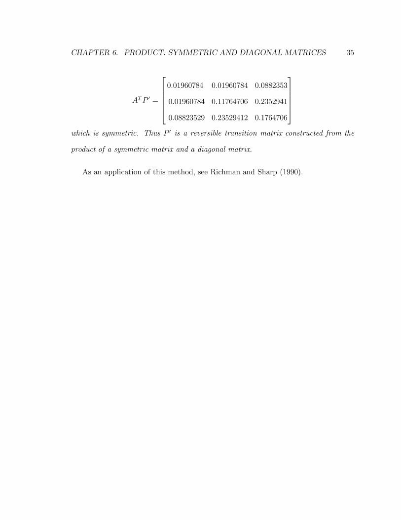
AT P ′ =
0.01960784 0.01960784 0.0882353
0.01960784 0.11764706 0.2352941
0.08823529 0.23529412 0.1764706
which is symmetric. Thus P ′ is a reversible transition matrix constructed from the
product of a symmetric matrix and a diagonal matrix.
As an application of this method, see Richman and Sharp (1990).

Chapter 7
Graph Method
7.1 Graph Method
Property 7.1.1. :
Consider an arbitrarily connected graph. A link between vertices i and j has weight
wij, with wji = wij, i, j ∈ S. Define the transition probabilities of a Markov chain by
pij =wij∑k wkk
. Then the Markov chain is reversible.
Proof. :
We guess that πi =
∑k wik∑
l
∑k wlk
, i, l, k ∈ S.
We interpret this as the proportion of time that the system is in state i, i.e., the
stationary probability of staying in state i.
It is easy to check that∑
i πi =
∑i
∑k wik∑
l
∑k wlk
= 1.
We find that
πipij =
∑k wik∑
l
∑k wlk
· wij∑k wik
=wij∑
l
∑k wlk
.
Similarly,
πjpji =
∑k wjk∑
l
∑k wlk
· wji∑k wjk
=wji∑
l
∑k wlk
=wij∑
l
∑k wlk
= πipij ,
36
CHAPTER 7. GRAPH METHOD 37
since wij = wji.
Further, we have shown that our guess and interpretation of πi is correct since the
stationary distribution is unique.
Thus we conclude that a Markov chain defined in such a way is reversible with
{πi} being the limiting probabilities.
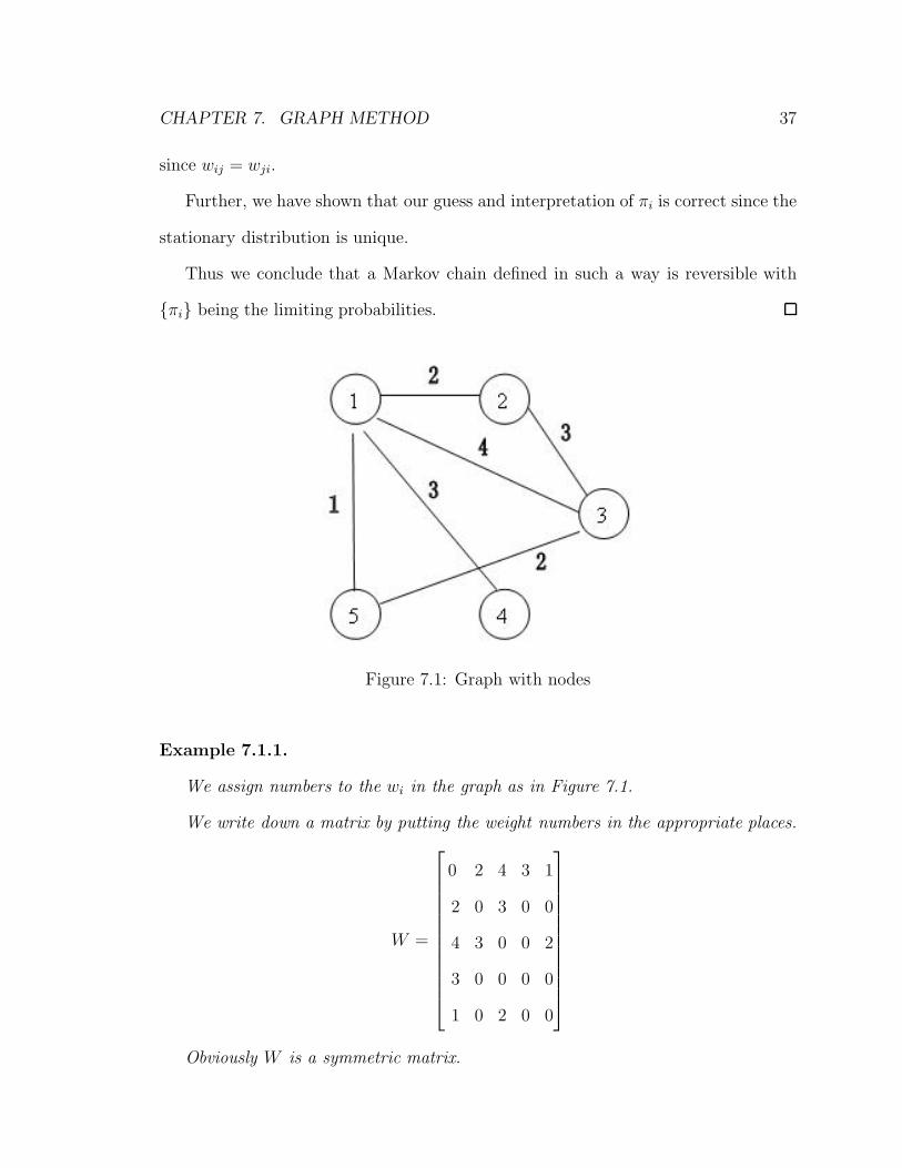
Figure 7.1: Graph with nodes
Example 7.1.1.
We assign numbers to the wi in the graph as in Figure 7.1.
We write down a matrix by putting the weight numbers in the appropriate places.
W =
0 2 4 3 1
2 0 3 0 0
4 3 0 0 2
3 0 0 0 0
1 0 2 0 0
Obviously W is a symmetric matrix.

CHAPTER 7. GRAPH METHOD 38
Next we scale the rows of W to convert it to a proper transition matrix P .
P =
0 210
410
310
110
25
0 35
0 0
49
39
0 0 29
33
0 0 0 0
13
0 23
0 0
.
By Property 7.1.1, P is reversible and the limiting probability of state i is πi =∑k wik∑
l
∑k wlk
. So
π1 =2 + 4 + 3 + 1
(2 + 4 + 3 + 1) + (2 + 3) + (3 + 4 + 2) + 3 + (1 + 2)=
1
3.
Similarly
π2 =1
6, π3 =
3
10, π4 =
1
10, π5 =
1
10.
We check the validity of limiting probabilities first.
Again using the limiting probability calculation method in chapter 1, we get
π1 = 0.3333333, π2 = 0.1666667, π3 = 0.3, π4 = 0.1, π5 = 0.1
which is consistent with the above results.
Then check the reversibility by computing (P 100)T P ,
(P 100)TP =
0 0.06666667 0.13333333 0.1 0.03333333
0.06666667 0 0.1 0 0
0.13333333 0.1 0 0 0.06666667
0.1 0 0 0 0
0.03333333 0 0.06666667 0 0
Since the resulting matrix is symmetric, the Markov chain with transition matrix
P is reversible.

Chapter 8
Tree Process
8.1 Definition
The following is from to Ross (2007).
Definition: “A Markov chain is said to be a tree process if
(i) pij > 0 whenever pji > 0,
(ii) for every pair of states i and j, i �= j,
there is a unique sequence of distinct states i = i0, i1, i2, · · · , in−1, in = j such that
pikik−1> 0, k = 0, 1, 2, · · · , n − 1
In other words, a Markov chain is a tree process if for every pair of distinct states i
and j, there is a unique way for the process to go from i to j without reentering a
state (and this path is the reverse of the unique path form j to i).”
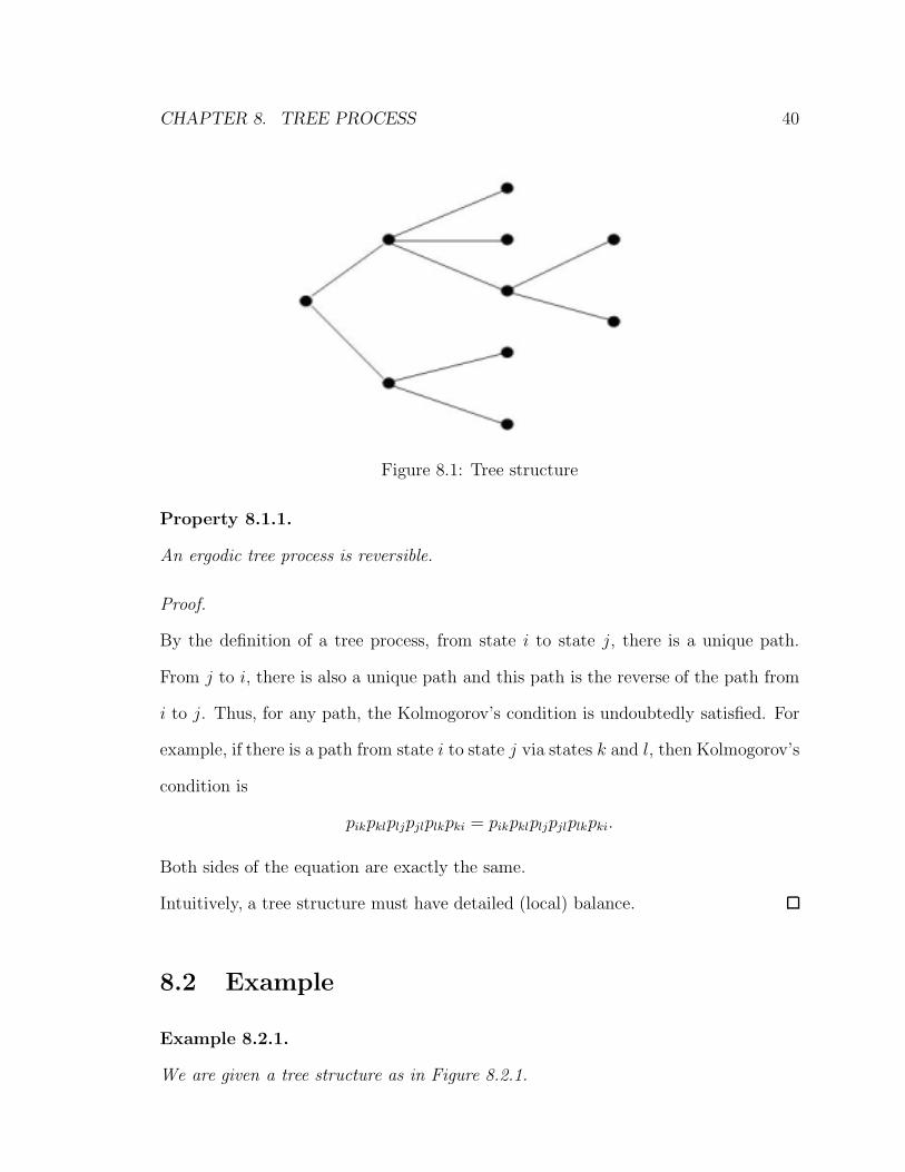
Graphically, the tree structure is a structure of the type shown in Figure 8.1,
where nodes stand for states.
The following is from Ross (2007).
39
CHAPTER 8. TREE PROCESS 40
Figure 8.1: Tree structure
Property 8.1.1.
An ergodic tree process is reversible.
Proof.
By the definition of a tree process, from state i to state j, there is a unique path.
From j to i, there is also a unique path and this path is the reverse of the path from
i to j. Thus, for any path, the Kolmogorov’s condition is undoubtedly satisfied. For
example, if there is a path from state i to state j via states k and l, then Kolmogorov’s
condition is
pikpklpljpjlplkpki = pikpklpljpjlplkpki.
Both sides of the equation are exactly the same.
Intuitively, a tree structure must have detailed (local) balance.
8.2 Example
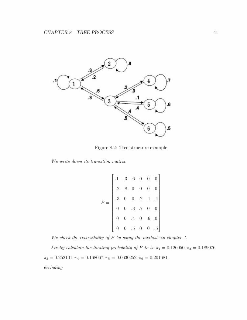
Example 8.2.1.
We are given a tree structure as in Figure 8.2.1.
CHAPTER 8. TREE PROCESS 41
Figure 8.2: Tree structure example
We write down its transition matrix
P =
.1 .3 .6 0 0 0
.2 .8 0 0 0 0
.3 0 0 .2 .1 .4
0 0 .3 .7 0 0
0 0 .4 0 .6 0
0 0 .5 0 0 .5
We check the reversibility of P by using the methods in chapter 1.
Firstly calculate the limiting probability of P to be π1 = 0.126050, π2 = 0.189076,
π3 = 0.252101, π4 = 0.168067, π5 = 0.0630252, π6 = 0.201681.
excluding
CHAPTER 8. TREE PROCESS 42
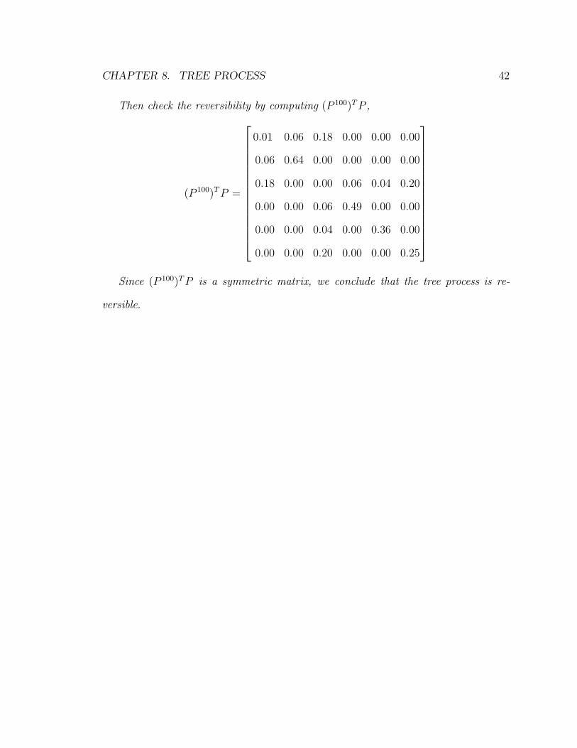
Then check the reversibility by computing (P 100)T P ,
(P 100)T P =
0.01 0.06 0.18 0.00 0.00 0.00
0.06 0.64 0.00 0.00 0.00 0.00
0.18 0.00 0.00 0.06 0.04 0.20
0.00 0.00 0.06 0.49 0.00 0.00
0.00 0.00 0.04 0.00 0.36 0.00
0.00 0.00 0.20 0.00 0.00 0.25
Since (P 100)T P is a symmetric matrix, we conclude that the tree process is re-
versible.
Chapter 9
Triangular completion method
9.1 Algorithm
1. We are given π (or choose π).
2. Choose probabilities for the upper triangular part (or lower triangular part),
excluding diagonals.
3. Calculate the lower triangular entries by the detailed balance equations of a
reversible process,
e.g.,
π2p21 = π1p12.
p21 =π1p12
π2
.
4. If row entries sum to less than (or equal to) 1, then set the diagonal entry so
that the row sums to 1. If a row has entries that sum to more than 1, scale the
row to make it sum to less than (or equal to) 1 and then set the diagonal entry
as in the previous case.
43
CHAPTER 9. TRIANGULAR COMPLETION METHOD 44
We have not seen this algorithm explicitly stated.
Property 9.1.1. The triangular completion method makes a reversible transition
matrix with a given limiting probability.
Proof.
Since we calculate the lower triangular entries from the detailed balance equation,
we have
πipij = πjpji ∀i, j
where either pij or pji is given and the other is computed.
Then we have
πipii0πi0pi0i1 · · ·πinpini = πipiinπinpinin−1 · · ·πi0pi0i.
Cancel out the π′s to get
pii0pi0i1 · · · pini = piinpinin−1 · · · pi0i. (9.1)
One thing that should be noted is that the computed entries are not necessarily
a probabilities since they are quite possibly greater than 1. But Equation (9.1) is
always true and we can scale the row (by multiplying by a constant less than 1) to
make sure that we have a valid transition matrix. Then Kolmogorov’s criterion is
satisfied so the resulting matrix is reversible.
9.2 Example
Example 9.2.1.
Step 1. We are given π = (.2, .1, .5, .2)

CHAPTER 9. TRIANGULAR COMPLETION METHOD 45
Step 2. Choose the upper triangular part, leaving the diagonal blank. Let
P =
.2 .1 .4
p21 .3 .5
p31 p32 .8
p41 p42 p43
Step 3. Calculate the lower triangular entries, i.e., the pij ’s (i > j), using the
detailed balance equations of a reversible process.
π2p21 = πip12
p21 =π1p12
π2=
.2(.2)
.1= .4
Similarly we get other p’s and the matrix P .
P =
.2 .1 .4
.4 .3 .5
.04 .06 .8
.4 .25 2
.
Step 4. Since the second row and the fourth row both sum to more than one, we
have to scale them. We multiply row two by ×0.5 (for example) and row four by
×0.25. Then we fill in the diagonal entries to make a valid transition matrix.
P ′ =
.3 .2 .1 .4
.2 .4 .15 .25
.04 .06 .1 .8
.1 .0625 .5 .3375
.
Now we check the reversibility of the transition matrix P ′ using the method of
Section 1.2.2.
CHAPTER 9. TRIANGULAR COMPLETION METHOD 46
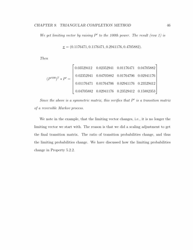
We get limiting vector by raising P ′ to the 100th power. The result (row 1) is
π = (0.1176471, 0.1176471, 0.2941176, 0.4705882).
Then
(P ′100)T ∗ P ′ =
0.03529412 0.02352941 0.01176471 0.04705882
0.02352941 0.04705882 0.01764706 0.02941176
0.01176471 0.01764706 0.02941176 0.23529412
0.04705882 0.02941176 0.23529412 0.15882353
Since the above is a symmetric matrix, this verifies that P ′ is a transition matrix
of a reversible Markov process.
We note in the example, that the limiting vector changes, i.e., it is no longer the
limiting vector we start with. The reason is that we did a scaling adjustment to get
the final transition matrix. The ratio of transition probabilities change, and thus
the limiting probabilities change. We have discussed how the limiting probabilities
change in Property 5.2.2.

Chapter 10
Convex Combination
10.1 Weighted Average
Property 10.1.1.
The convex combination of two reversible Markov transition matrices with the
same stationary distribution π, is reversible, and the stationary distribution remains
the same.
Proof.
Let A = {aij} and B = {bij} be the transition matrices of two reversible processes.
Let P be a convex combination of A and B.
P = αA + (1 − α)B, α ∈ [0, 1].
Then P is a transition matrix since
∑j
pij = α∑
j
aij + (1 − α)∑
j
bij = 1
Further,
πP = π(αA + (1 − α)B) = απA + (1 − α)πB = απ + (1 − α)π = π,
47

CHAPTER 10. CONVEX COMBINATION 48
πipij = απiaij + (1 − α)πibij
= απjaji + (1 − α)πjbji, since A and B are reversible
= πj(αaji + (1 − α)bji)
= πjpji.
Thus, P is reversible.
10.2 Example
Example 10.2.1. We will use the examples from section 5.1 on the Symmetric Pairs
Scaling method.
A =
.25 .25 .25 .25
.3 .1 .3 .3
.15 .15 .55 .15
.1 .1 .1 .7
,
and
B =
.125 .125 .5 .25
.15 .1 .3 .45
.3 .15 .4 .15
.1 .15 .1 .65
,
A and B have the same limiting vector
π = (0.1666667, 0.1388889, 0.2777778, 0.4166667)
Let P be the convex combination of A and B,
P = 0.3 ∗ A + 0.7 ∗ B

CHAPTER 10. CONVEX COMBINATION 49
=
0.1625 0.1625 0.425 0.250
0.1950 0.1000 0.300 0.405
0.2550 0.1500 0.445 0.150
0.1000 0.1350 0.100 0.665
We now find out the limiting vector of P and check its reversibility using the method
from Section 1.2.2.
Calculating P 100, we get the limiting vector of P as
π = (0.1666667, 0.1388889, 0.2777778, 0.4166667),
and
(P 100)T ∗ P =
0.02708333 0.02708333 0.07083333 0.04166667
0.02708333 0.01388889 0.04166667 0.05625000
0.07083333 0.04166667 0.12361111 0.04166667
0.04166667 0.05625000 0.04166667 0.27708333
.
This is symmetric, and verifies that P, the convex combination of two reversible ma-
trices, is reversible.
Corollary 10.3. The convex combination of a countable collection of reversible ma-
trices is reversible, i.e.,
P = α0P0 + α1P1 + α2P2 + α3P3 + · · ·
is reversible, where
i) {Pi}, i = 0, 1, 2, 3, · · · are reversible Markov transition matrices, and
ii)∑
i αi = 1, 1 ≥ αi ≥ 0.
Chapter 11
Reversibility and Invariance
The following two properties are stated (without proof) and are taken from Strook
(2005). The proofs given are ours. Let P be the transition matrix of a Markov chain.
Let P ∗ be the transition matrix for the reversed Markov chain. It is know that both
matrices have the same limiting vector. The limiting vector of P is invariant under
the construction of the two reversible transition matrices in the next two properties.
11.1 P+P ∗2
Property 11.1.1. Let P be any transition matrix with limiting vector π. Define
P ∗ = {qij} where qij =πj
πipji. Then P+P∗
2is reversible with limiting vectorπ.
Proof.
First P and P ∗ have the same limiting probabilities.
A weighted average of two transition matrices with the same limiting probability vec-
tor is a transition matrix with the same limiting probability vector.
50

CHAPTER 11. REVERSIBILITY AND INVARIANCE 51
Let M = [mij] = P+P∗2
= [pij
2+
πj
2πipji]. Clearly
mij =pij
2+
πj
2πipji ≥ 0.
Then
∑j
mij =∑
j
pij
2+
∑j
πj
2πipji
=1
2
∑j
pij +1
2πi
∑j
πjpji
=1
2+
πi
2πi
= 1
where ∑j
πjpji = πi, since πP = π.
Thus, P+P∗2
is a transition matrix.
Further, by the definition of P ∗, it is the transition matrix of the reversed process
defined by P . So P ∗ has the same stationary distribution as P . So
πM =πP + πP ∗
2=
π + π
2= π.
Lastly, we check the detailed balance equations for P+P∗2
.
πimij = πi(pij
2+
πj
2πipji)
=1
2(πipij + πjpji)
= πj(πi
2πjpij +
pji
2)
= πjmji.
Therefore, we can conclude that P+P∗2
is a transition matrix defined by a reversible
Markov process which has π as its limiting probability.

CHAPTER 11. REVERSIBILITY AND INVARIANCE 52
Example 11.1.1. Consider a transition matrix
P =
.2 .4 .4
.3 .2 .5
.3 .3 .4
,
which has limiting vector as π = [ 33121
, 36121
, 52121
]. We can check that P is not reversible.
Then we construct another transition matrix P ∗ = {qij} by the rule qij =πj
πipji:
P ∗ =
15
1855
2655
1130
15
1330
33130
45130
25
.
Thus we get the following result using R:
P + P ∗
2=
0.2000000 0.3636364 0.4363636
0.3333333 0.2000000 0.4666667
0.2769231 0.3230769 0.4000000
.
The limiting vector of P+P∗2
is
(P + P ∗
2)100 =
0.2727273 0.2975207 0.4297521
0.2727273 0.2975207 0.4297521
0.2727273 0.2975207 0.4297521
,
and checking the reversibility of P+P∗2
we get
((P + P ∗
2)100)T ∗ P + P ∗
2=
0.05454545 0.09917355 0.1190083
0.09917355 0.05950413 0.1388430
0.11900826 0.13884298 0.1719008
We see that P+P∗2
is a reversible transition matrix which has the same limiting
vector as P .

CHAPTER 11. REVERSIBILITY AND INVARIANCE 53
11.2 P ∗P
Property 11.2.1. Let P be any transition matrix with limiting vector π. Define P ∗ =
{qij} where qij =πj
πipji. Then P ∗P is reversible with the same limiting probability
vector as P .
Proof.
First, the product of two transition matrices is a transition matrix, since it repre-
sents a two step transition with two different matrices. If π is the limiting vector for
P , then π is also the limiting vector for P ∗ since P ∗ is the transition matrix for the
reverse Markov chain.
Let R = P ∗P. Then
∑j
rij =∑
j
∑k
qikpkj
=∑
k
∑j
qikpkj
=∑
k
qik
∑j
pkj
=∑
k
qik = 1.
Further,
πP ∗P = πP = π.
Then
πirij = πi
∑k
qikpkj
= πi
∑k
πk
πipkipkj
= πj
∑k
πk
πjpkjpki
= πj
∑k
qjkpki = πjrji.
So P ∗P is a reversible transition matrix with same limiting vector as P .

CHAPTER 11. REVERSIBILITY AND INVARIANCE 54
Example 11.2.1. We again use the P and P ∗ of our last example.
P =
.2 .4 .4
.3 .2 .5
.3 .3 .4
and P ∗ =
15
1855
2655
1130
15
1330
33130
45130
25
.
Then
P ∗P =
0.2800000 0.2872727 0.4327273
0.2633333 0.3166667 0.4200000
0.2746154 0.2907692 0.4346154
.
The limiting probability of P ∗P is calculated as
(P ∗P )100 =
0.2727273 0.2975207 0.4297521
0.2727273 0.2975207 0.4297521
0.2727273 0.2975207 0.4297521
,
and checking the reversibility of P ∗P using Section 1.2.2 yields
((P ∗P )100)T ∗ (P ∗P ) =
0.07636364 0.07834711 0.1180165
0.07834711 0.09421488 0.1249587
0.11801653 0.12495868 0.1867769
We can find that P ∗P is reversible and has the same limiting vector as transition
matrix P .
This chapter shows interesting methods which allow us to construct reversible
matrices from non-reversible matrices and still retain the same stationary distribution.

Chapter 12
Expand and Merge Methods
12.1 State by State Expand
Property 12.1.1. Given an n × n reversible Markov transition matrix P , we can
expand it to an (n+ 1)× (n+1) reversible Markov transition matrix Q by setting the
proper transition rates.
We show this method with an example.
Example 12.1.1. We begin with P , the transition matrix of a reversible Markov
chain with 3 states.
P =
.5 .3 .2
.3 .3 .4
.1 .2 .7
We want to expand it by one more state to get a 4 × 4 transition matrix.
55
CHAPTER 12. EXPAND AND MERGE METHODS 56
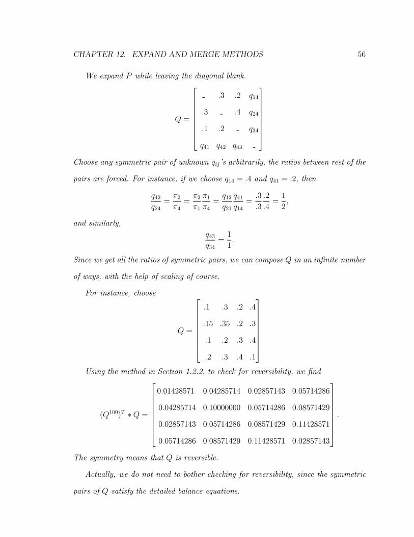
We expand P while leaving the diagonal blank.
Q =
.3 .2 q14
.3 .4 q24
.1 .2 q34
q41 q42 q43
Choose any symmetric pair of unknown qij’s arbitrarily, the ratios between rest of the
pairs are forced. For instance, if we choose q14 = .4 and q41 = .2, then
q42
q24
=π2
π4
=π2
π1
π1
π4
=q12
q21
q41
q14
=.3
.3
.2
.4=
1
2,
and similarly,
q43
q34=
1
1.
Since we get all the ratios of symmetric pairs, we can compose Q in an infinite number
of ways, with the help of scaling of course.
For instance, choose
Q =
.1 .3 .2 .4
.15 .35 .2 .3
.1 .2 .3 .4
.2 .3 .4 .1
Using the method in Section 1.2.2, to check for reversibility, we find
(Q100)T ∗ Q =
0.01428571 0.04285714 0.02857143 0.05714286
0.04285714 0.10000000 0.05714286 0.08571429
0.02857143 0.05714286 0.08571429 0.11428571
0.05714286 0.08571429 0.11428571 0.02857143
.
The symmetry means that Q is reversible.
Actually, we do not need to bother checking for reversibility, since the symmetric
pairs of Q satisfy the detailed balance equations.

CHAPTER 12. EXPAND AND MERGE METHODS 57
12.2 Merge Method
This is our last method to construct transition matrices of reversible Markov chains.
Yet it is the most expandable since it can glue any number of reversible Markov
processes together to form a new reversible process which has a larger state space.
We demonstrate this method with an example first.
Figure 12.1: Process A
Example 12.2.1.
We are given two reversible processes which have A and B as their transition
matrix respectively.
A =
.2 .4 .4
.35 .3 .35
.2 .2 .6

CHAPTER 12. EXPAND AND MERGE METHODS 58
and
B =
.2 .3 .3 .2
.2 .4 .2 .2
.1 .1 .7 .1
.2 .3 .3 .2
.
Graphically, processes A and B can be shown as in Figure 12.2 and Figure 12.2.1.
Figure 12.2: Process B
If we glue these two processes at state 3 of Process A and state 1 of Process B,
the combination graph would be shown in Figure 12.3.
Then what will the new transition matrix be like?
Since the ratios between all transition probabilities are not affected by the merge,
we keep the pij ’s remaining the same and leave the diagonal entry of knot state, p33,
blank temporarily.

CHAPTER 12. EXPAND AND MERGE METHODS 59
Figure 12.3: Merged graph
Write down the new transition matrix P ′ as
P ′ =
.2 .4 .4 0 0 0
.35 .3 .35 0 0 0
.2 .2 .3 .3 .2
0 0 .2 .4 .2 .2
0 0 .1 .1 .7 .1
0 0 .2 .3 .3 .2
We find that the third row sums to more than one, thus we scale it by multiplying
by a factor, say 0.6. We choose the diagonal so that the row sums to 1. We get a

CHAPTER 12. EXPAND AND MERGE METHODS 60
final transition matrix
P =
.2 .4 .4 0 0 0
.35 .3 .35 0 0 0
.12 .12 .28 .18 .18 .12
0 0 .2 .4 .2 .2
0 0 .1 .1 .7 .1
0 0 .2 .3 .3 .2
Check the reversibility of P using the method in Section 1.2.2.
(P 100)T ∗ P =
0.01213873 0.02427746 0.02427746 0.00000000 0.00000000 0.00000000
0.02427746 0.02080925 0.02427746 0.00000000 0.00000000 0.00000000
0.02427746 0.02427746 0.05664740 0.03641618 0.03641618 0.02427746
0.00000000 0.00000000 0.03641618 0.07283237 0.03641618 0.03641618
0.00000000 0.00000000 0.03641618 0.03641618 0.25491329 0.03641618
0.00000000 0.00000000 0.02427746 0.03641618 0.03641618 0.02427746
We get a symmetric matrix and conclude that P is reversible.
Now we are back to state this method and prove it.
Property 12.2.1.
A process glued from any two reversible Markov processes is reversible.
Proof. We are given two reversible Markov transition matrices A = [aij] which has n
states and B = [bij] which has m states.
If we glue any two states of processes A and B together, say state k of A and state
l of B together, we will have a (m + n − 1) state space S.

CHAPTER 12. EXPAND AND MERGE METHODS 61
Choose any path of S starting with any state and returning to that same state,
eg. A path starts from state i of process A. So the Kolmogorov condition product
has probability
aii0ai0i1 · · · airkblj0bj0j1 · · · bj0lakirairir−1 · · · ai0i.
The reversed path has the identical probability as the original path since both A and
B are reversible.
Thus the Kolmogorov condition is satisfied for the glued process and thus the
glued process is reversible. The scaling adjustment does not affect the reversibility as
we have already seen.

Chapter 13
Summary
In this paper, we gave numerous methods (some known and many new) to create
transition matrices for reversible Markov chains. We also gave operations on such
matrices which will maintain the reversible nature of Markov chains. We used count-
ing arguments to find the number of equations that are needed to check whether a
Markov Chains is reversible using the Kolmogorov condition. We present a practical
computer based method for checking whether or not small dimensional transition ma-
trices correspond to reversible Markov chains. Since reversible Markov Chains appear
frequently in the literature, we believe that this paper is a valuable contribution to
the area.
62

Bibliography
[1] Aldous, D. and Fill, J. (2002). Reversible Markov Chains and Random Walks on
Graphs. http://www.stat.berkeley.edu/∼aldous/RWG/book.html
[2] Allen, L.J.S., (2003). An Introduction to Stochastic Processes with Applications to
Biology. Pearson.
[3] Evans, M.J. and Rosenthal, J.S. (2004). Probability and Statistics: The Science
of Uncertainty. W.H. Freeman.
[4] Jain, J.L., Mohanty, S.G., Bohr, W. (2006). A Course on Queueing Models. CRC
Press.
[5] Kao, E. (1997). An Introduction to Stochastic Processes. Duxbury Press.
[6] Kelly, F.P. (1979). Reversibility and Stochastic Networks. Wiley.
[7] Kijima, M. (1997). Markov processes for stochastic modeling. CRC Press.
[8] Nelson, R. (1995). Probability, stochastic processes, and queueing theory. Springer.
[9] Ross, S.M. (2002). Probability models for computer science. Academic Press.
[10] Ross, S.M. (2007). Introduction to probability models, 9th Edition. Academic
Press.
63
BIBLIOGRAPHY 64
[11] Richman, D. and Sharp, W.E. (1990). A method for determining the reversibility
of a Markov Sequence. Mathematical Geology, Vol.22, 749-761.
[12] Rubinstein, Y.R. and Kroese, D.P. (2007). Simulation and the Monte Carlo
Method, 2nd edition. Wiley.
[13] Strook, D.W. (2005). Introduction to Markov Chains. Birkhuser.
[14] Wolff, R.W. (1989). Stochastic Modeling and the Theory of Queues. Prentice
Hall.