construction of polygonal interpolants: a maximum entropy...

INTERNATIONAL JOURNAL FOR NUMERICAL METHODS IN ENGINEERINGInt. J. Numer. Meth. Engng 2004; 61:2159–2181Published online in Wiley InterScience (www.interscience.wiley.com). DOI: 10.1002/nme.1193

Construction of polygonal interpolants: a maximumentropy approach

N. Sukumar∗,†

Department of Civil and Environmental Engineering, University of California, Davis, CA 95616, U.S.A.

SUMMARY

In this paper, we establish a link between maximizing (information-theoretic) entropy and the con-struction of polygonal interpolants. The determination of shape functions on n-gons (n > 3) leadsto a non-unique under-determined system of linear equations. The barycentric co-ordinates i , whichform a partition of unity, are associated with discrete probability measures, and the linear reproducingconditions are the counterpart of the expectations of a linear function. The i are computed bymaximizing the uncertainty H(1, 2, . . . , n) = −∑n

i=1 i log i , subject to the above constraints.The description is expository in nature, and the numerical results via the maximum entropy (MAXENT)formulation are compared to those obtained from a few distinct polygonal interpolants. The maxi-mum entropy formulation leads to a feasible solution for i in any convex or non-convex polygon.This study is an instance of the application of the maximum entropy principle, wherein least-biasedinference is made on the basis of incomplete information. Copyright 2004 John Wiley & Sons, Ltd.

KEY WORDS: Shannon entropy; information theory; barycentric co-ordinates; natural neighbours;Laplace interpolant; meshfree interpolant; data interpolation

1. INTRODUCTION

In information theory, the notion of entropy as a measure of uncertainty or incomplete knowl-edge was introduced by Shannon [1]. The quantity H(p1, p2, . . . , pn) = −∑n

i=1 pi log pi wasreferred to as the informational entropy of an ensemble, where pi is the probability asso-ciated with the occurrence of the event xi , subject to the condition

∑ni=1 pi = 1. Building

on Shannon’s work, Jaynes [2, 3] proposed the principle of maximum entropy (MAXENT), inwhich through its bearing on well-known ensemble distributions in statistical mechanics, it wasshown that maximizing H was the least-biased means to obtain rational (statistical) inference

∗Correspondence to: N. Sukumar, Department of Civil and Environmental Engineering, University of California,One Shields Avenue, Davis, CA 95616, U.S.A.

†E-mail: [email protected]

Contract/grant sponsor: National Science Foundation; contract/grant number: contract CMS–0352654

Received 23 January 2004Revised 3 June 2004

Copyright 2004 John Wiley & Sons, Ltd. Accepted 9 July 2004

2160 N. SUKUMAR

in the face of insufficient data. Jaynes [4] presents a concise and transparent explanation ofthe MAXENT formalism (Jaynes’s principle). We point out that the meaning of entropy within thecontext of MAXENT is to be viewed in the information-theoretic sense, as opposed to the conceptof entropy which arises in thermodynamics and statistical physics, where it is a measure of theequilibria and evolution of thermodynamic systems. The application of the principle of maximumentropy has touched many disciplines, ranging from economics to statistical mechanics, imageenhancement to nuclear physics, and as diverse as urban planning and biology. The collection ofJaynes’s papers in Reference [5] provide a chronological sequence of progress in the evolutionof maximum entropy methods, whereas Khinchin [6] presents the mathematical roots and basisof information theory. For a description of the various applications of MAXENT in science andengineering, the interested reader can refer to Kapur [7].

In this paper, we view the data interpolation problem in a new light, and apply the maxi-mum entropy principle to obtain least-biased interpolants on polygonal domains. To the author’sknowledge, such an approach has not been pursued previously. The only study that does adoptthe principle of maximum entropy with finite elements is the work of Beltzer [8]. In Ref-erence [8], the MAXENT principle was used to characterize finite elements in terms of itscomplexity. Even though the use of the maximum entropy principle has primarily been ap-plied to problems associated with randomness, such a notion is not necessarily required [4].The MAXENT principle is equally applicable to any inferential problem with incomplete data,in which the minimally prejudiced (maximally non-committal) solution is sought. This is theviewpoint adopted in this study. The author’s recent research on the development of a naturalneighbour-based polygonal finite element method [9] and its use to construct a conforming h-adaptive finite element method on tree-based meshes [10] provided impetus to pursue the presentinvestigation.

The outline of this paper is as follows. In Section 2, the maximum entropy principle forthe polygonal interpolant problem is presented, and in Section 3 its solution is obtainedby using the method of Lagrange multipliers combined with a numerical scheme in whichthe minimizer of a convex function is sought. In Section 4, numerical results using theMAXENT principle are presented for both, convex and non-convex polygons, and compar-isons are made to results obtained from a few recently developed polygonal interpolants (seeReference [9] for details). The main results and conclusions from this study are indicated inSection 5.

2. PROBLEM STATEMENT AND FORMULATION

Consider a microscopic ensemble in which the sample space consists of mutually inde-pendent discrete events x1, x2, . . . , xn that occur with probabilities p1, p2, . . . , pn, respectively.Since in a random experiment, P() = 1, it follows that the non-negative probabilities pi mustsatisfy the condition

∑i pi = 1. Now, consider m (m < n − 1) macroscopic observations, in

which the expected value of a function gr(x) (denoted by 〈gr(x)〉) is known. Then, the mostlikely probability distribution pi is obtained by maximizing the informational entropy H(·)[1, 2]

Maximize

(H(p1, p2, . . . , pn) = −

n∑i=1

pi log pi

)(1a)

Copyright 2004 John Wiley & Sons, Ltd. Int. J. Numer. Meth. Engng 2004; 61:2159–2181

CONSTRUCTION OF POLYGONAL INTERPOLANTS 2161

Ωe

p

1

34

2

Ω ep 36

5

4

12

(a) (b)

Figure 1. Approximation at point p in an n-gon: (a) square (n = 4); and (b) hexagon (n = 6).

subject to the constraintsn∑

i=1pi = 1 (1b)

n∑i=1

pigr(xi) = 〈gr(x)〉 (1c)

where log .= 0 if = 0 and the specific form of the uncertainty measure H(·) given

in Equation (1a) is based on the satisfaction of three conditions, namely, H is a continuousfunction of the pi , it attains its maximum when pi = 1/n ∀i with the maximum entropyHmax = H(1/n, . . . , 1/n) a monotonic function, and the composition law must hold [1, 2]. Theabove form of H guarantees that pi 0. The solution for pi is obtained using the method ofLagrange multipliers, which we leave for a later stage when the specific polygonal interpolationproblem is considered. The rationale for using MAXENT rests on the fact that the entropy of mostof the admissible distributions that satisfy the constraints are concentrated in the neighbourhoodof the maximum entropy [11], and hence the maximum entropy distribution is the least-biasedand the one that has the maximum likelihood to occur.

We now draw an analogy between the above problem and the polygonal interpolation one,which forms the basis of the approach pursued in this study. For details on the propertiesassociated with barycentric co-ordinates on polygons we refer the reader to Sukumar andTabarraei [9]; here we only mention relations that are directly pertinent to our investigation.Consider the n-gons shown in Figure 1, where the nodes are located at the vertices of thepolygons. To each node, we associate a shape function (barycentric co-ordinate) i 0 in e.Consider a point p in e with co-ordinate x ≡ (x, y). The interpolant uh(x) for a scalar-valuedfunction u(x) : e → R can be written as

uh(x) =n∑

i=1i (x)ui (2)

where ui = u(xi ) are the prescribed nodal values of u(x). The property i 0 (convex combina-tion) ensures that the interpolant satisfies a discrete maximum principle: mini ui uh maxi ui .We now impose the restriction that the i are such that uh(x) can exactly reproduce constant


2162 N. SUKUMAR

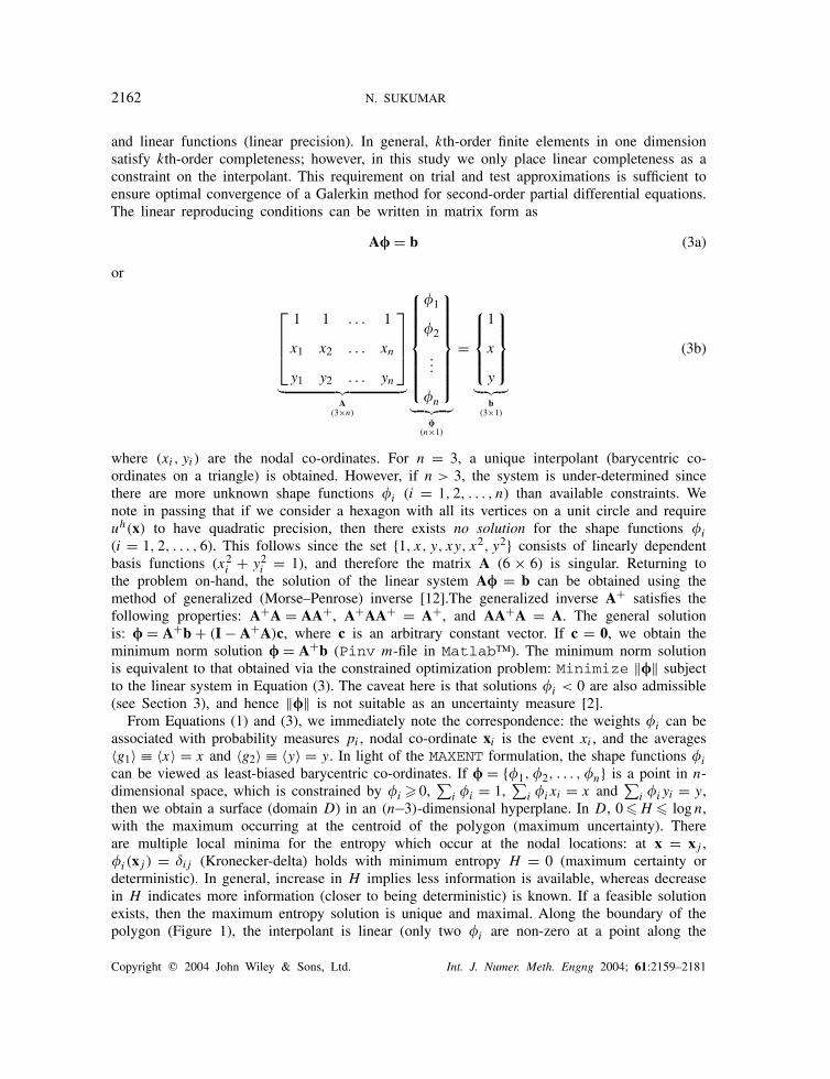
and linear functions (linear precision). In general, kth-order finite elements in one dimensionsatisfy kth-order completeness; however, in this study we only place linear completeness as aconstraint on the interpolant. This requirement on trial and test approximations is sufficient toensure optimal convergence of a Galerkin method for second-order partial differential equations.The linear reproducing conditions can be written in matrix form as

A = b (3a)

or

1 1 . . . 1

x1 x2 . . . xn

y1 y2 . . . yn

︸︷︷︸A

(3×n)

1

2

...

n

︸︷︷︸

(n×1)

=

1

x

y

︸︷︷︸

b(3×1)

(3b)

where (xi, yi) are the nodal co-ordinates. For n = 3, a unique interpolant (barycentric co-ordinates on a triangle) is obtained. However, if n > 3, the system is under-determined sincethere are more unknown shape functions i (i = 1, 2, . . . , n) than available constraints. Wenote in passing that if we consider a hexagon with all its vertices on a unit circle and requireuh(x) to have quadratic precision, then there exists no solution for the shape functions i

(i = 1, 2, . . . , 6). This follows since the set 1, x, y, xy, x2, y2 consists of linearly dependentbasis functions (x2

i + y2i = 1), and therefore the matrix A (6 × 6) is singular. Returning to

the problem on-hand, the solution of the linear system A = b can be obtained using themethod of generalized (Morse–Penrose) inverse [12].The generalized inverse A+ satisfies thefollowing properties: A+A = AA+, A+AA+ = A+, and AA+A = A. The general solutionis: = A+b + (I − A+A)c, where c is an arbitrary constant vector. If c = 0, we obtain theminimum norm solution = A+b (Pinv m-file in Matlab™). The minimum norm solutionis equivalent to that obtained via the constrained optimization problem: Minimize ‖‖ subjectto the linear system in Equation (3). The caveat here is that solutions i < 0 are also admissible(see Section 3), and hence ‖‖ is not suitable as an uncertainty measure [2].

From Equations (1) and (3), we immediately note the correspondence: the weights i can beassociated with probability measures pi , nodal co-ordinate xi is the event xi , and the averages〈g1〉 ≡ 〈x〉 = x and 〈g2〉 ≡ 〈y〉 = y. In light of the MAXENT formulation, the shape functions i

can be viewed as least-biased barycentric co-ordinates. If = 1, 2, . . . , n is a point in n-dimensional space, which is constrained by i 0,

∑i i = 1,

∑i ixi = x and

∑i iyi = y,

then we obtain a surface (domain D) in an (n−3)-dimensional hyperplane. In D, 0 H log n,with the maximum occurring at the centroid of the polygon (maximum uncertainty). Thereare multiple local minima for the entropy which occur at the nodal locations: at x = xj ,i (xj ) = ij (Kronecker-delta) holds with minimum entropy H = 0 (maximum certainty ordeterministic). In general, increase in H implies less information is available, whereas decreasein H indicates more information (closer to being deterministic) is known. If a feasible solutionexists, then the maximum entropy solution is unique and maximal. Along the boundary of thepolygon (Figure 1), the interpolant is linear (only two i are non-zero at a point along the



interior of the edges of the polygon). The above inferences that we have drawn on the MAXENTinterpolant were also true for the polygonal interpolants considered in Reference [9], which inpart provided motivation to pursue the present investigation.

2.1. Method of Lagrange multipliers

We can now state the polygonal interpolation problem using the MAXENT formulation. We seekto find i (i = 1, 2, . . . , n) that are the solution of the following problem:

Maximize

(H(1, 2, . . . , n) = −

n∑i=1

i log i

)(4a)

subject to the linear constraints

n∑i=1

i = 1 (4b)

n∑i=1

ixi = x (4c)

n∑i=1

iyi = y (4d)

where (x, y) ∈ e (interior of the polygon). On the boundary of the convex hull, the MAXENTsolution for i is known. We use the method of Lagrange multipliers to solve the constrainedoptimization problem. Let r (r = 0, 1, 2) be the Lagrange multipliers associated with the threeconstraints, and we set the variation of the augmented Lagrangian to zero (L = 0) [2]

[n∑

i=1− i log i + 0

(1 −

n∑i=1

i

)+ 1

(x −

n∑i=1

ixi

)+ 2

(y −

n∑i=1

iyi

)]= 0 (5)

or

[−1 − log i − 0 − 1xi − 2yi]i = 0 ∀i (6)

and since the variations i are arbitrary, we obtain

−1 − log i − 0 − 1xi − 2yi = 0 (i = 1, 2, . . . , n) (7)

In keeping with convention, we let 0 = log Z−1 [2]. The function Z is known as the partitionfunction, and is used to represent the canonical distribution in statistical mechanics. Then, theabove equation can be written as

log i + log Z = −1xi − 2yi (8)

or

i = e−1xi−2yi

Z(9)


2164 N. SUKUMAR

and since∑

i i = 1, we have

Z(1, 2) =n∑

i=1e−1xi−2yi (10)

and therefore the shape functions i can be written as

i = e−1xi−2yi∑nj=1 e−1xj −2yj

≡ Zi∑nj=1 Zj

(11)

where Zi can be viewed as a weight function, and the last expression is a common form inwhich most polygonal interpolation schemes appear [9]. Now, to complete the formulation, thei must satisfy the constraints given in Equations (4c) and (4d). The constraints can also bewritten as [2]

−0

r

= −(log Z)

r

= 〈gr(x)〉, (r = 1, 2) (12)

where 〈g1(x)〉 = x and 〈g2(x)〉 = y. On substituting Equation (11) in Equations (4c) and (4d),we obtain the following non-linear equations for 1 and 2:

f1(1, 2) = 0, f2(1, 2) = 0 (13a)

where

f1(1, 2) =∑n

i=1 e−1xi−2yi xi

Z− x (13b)

f2(1, 2) =∑n

i=1 e−1xi−2yi yi

Z− y (13c)

and on solving for 1 and 2, the shape functions i are obtained from Equation (11). Onusing Equations (11) and (4a), the maximum entropy is: Hmax = log Z(1, 2) + 1x + 2y.

Note that Equation (13) defines a non-linear mapping: x = x(1, 2), y = y(1, 2), which isused in Section 4.3 to derive the derivatives of the shape functions.

2.1.1. Nearest-neighbour interpolation. If the only constraint is∑

i i = 1 (constant precision),then from Equation (11) with r (r = 1, 2) set to zero, we obtain

i = 1

n∀i (14)

which is the nearest-neighbour interpolant. The shape functions are a constant over the polygon.

2.1.2. Bilinear interpolation. Consider the unit square shown in Figure 1(a). Let the domaine = (0, 1)2 with the origin at node 1. For a point p in e with co-ordinate (x, y), we use



Equation (13) to obtain the following equations for 1 and 2:

e−1 + e−1−2

1 + e−1 + e−2 + e−1−2= x (15a)

e−2 + e−1−2

1 + e−1 + e−2 + e−1−2= y (15b)

which simplifies to

e−1

1 + e−1= x (16a)

e−2

1 + e−2= y (16b)

and therefore

e−1 = x

1 − x, e−2 = y

1 − y(17)

From Equations (10) and (17), we have Z−1 = (1 − x)(1 − y) and on using Equation (11), weobtain the MAXENT shape functions

1(x, y) = (1 − x)(1 − y), 2(x, y) = x(1 − y), 3(x, y) = xy, 4(x, y) = y(1 − x)

(18)

which are identical to bilinear finite element shape functions.

3. NUMERICAL ALGORITHM

The non-linear equations in Equation (13) immediately suggest the use of an iterative solutionscheme such as Newton’s method. However, to solve Equation (13) without cognizance of itsspecial structure is fraught with numerical difficulties. As is well-known, Newton’s method forroot finding is sensitive (especially so in multi-dimensions) to the initial guess. Numerical testshave revealed that convergence is realized if and only if the initial guess is proximal to theexact solution, and as the point p(x, y) approaches the boundary of the domain, the situationis exacerbated and non-convergence or even convergence to the wrong solution results.

The fact that Equation (13) arises from a maximum entropy formalism suggests that there ismore information in fr that one can use. This fact was used by Agmon and co-workers [13, 14]towards the development of a suitable algorithm to find the distribution of maximum entropy.In Reference [15], the maximum entropy (primal) problem is recast into one (dual problem)in which the Lagrange multipliers are determined as the set that minimizes a convex potentialfunction F(1, 2). A brief description of the algorithm follows. On noting that

∑i i = 1

and letting xi = xi − x and yi = yi − y, we can re-write the linear reproducing conditions in


2166 N. SUKUMAR

Equations (4c) and (4d) as

n∑i=1

i xi = 0 (19a)

n∑i=1

i yi = 0 (19b)

which can be viewed as using a shifted co-ordinate system with the origin placed at (x, y).This choice is preferred in numerical computations since it is more stable than the form thatappears in Equation (4). Now, the expressions for Z and i take the form

Z(1, 2) =n∑

i=1e−1xi−2yi , i = e−1xi−2yi

Z(20)

where the Lagrange multipliers 1 and 2 remain unchanged, and there is a change only in 0

with the new value 0 = 0 + 1x + 2y. We note that e−1xi−2yi = e−1xi−2yi · e1x+2y , andtherefore the equality between the expressions for i in Equations (11) and (20) is apparent.In addition, the maximum entropy is now given by Hmax = log Z(1, 2). Instead of Equation(13), we now have [14]

fr(1, 2) = (log Z)

r

= 0, (r = 1, 2) (21a)

f1(1, 2) = −∑n

i=1 e−1xi−2yi xi

Z(21b)

f2(1, 2) = −∑n

i=1 e−1xi−2yi yi

Z(21c)

Since f1(1, 2) ≡ F/1 = 0 and f2(1, 2) ≡ F/2 = 0, we note that f is a conservativevector field with scalar potential f = ∇ log Z(1, 2) ≡ ∇F(1, 2) [14]. In addition, as Z > 0,the above equations can also be written as

fr(1, 2) = Z

r

= 0, (r = 1, 2) (22a)

f1(1, 2) = −n∑

i=1e−1xi−2yi xi (22b)

f2(1, 2) = −n∑

i=1e−1xi−2yi yi (22c)

where now f = ∇Z(1, 2) ≡ ∇F (1, 2). Let t ≡ (t1,

t2) denote any trial set of Lagrange

multipliers and the set ≡ (1, 2) be the one that maximizes the entropy (since F() = Hmax).



In the dual problem, the point x is fixed, and the Lagrange multipliers are varied, as opposed tothe primal formulation in which the constraint equations define a mapping from the point x tothe solution set and vice versa. The positive-definiteness of F was established in Reference[15] (see Section 4.3 for the derivation of the Hessian of log Z), and consequently F attainsa global minimum at t = . Since is the minimizer of both F and F , we now show thatF = Z(t) attains a global minimum at t = for the polygonal interpolation problem.

Claim 1The function F = Z(t) attains a global minimum at t = .

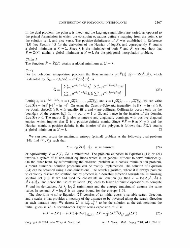
ProofFor the polygonal interpolation problem, the Hessian matrix of F (t

1, t2) = Z(t

1, t2), which

is denoted by Grs = fr/ts = 2

F /trt

s , is

G =∑n

i=1 e−1xi−2yi x2i

∑ni=1 e−1xi−2yi xi yi∑n

i=1 e−1xi−2yi xi yi

∑ni=1 e−1xi−2yi y2

i

(23)

Letting ai = e−1xi−2yi , u = (√

a1x1, . . . ,√

anxn), and v = (√

a1y1, . . . ,√

anyn), we can writedet(G) = ‖u‖2‖v‖2 − |u · v|2. On using the Cauchy–Schwartz inequality, ‖u‖‖v‖− |u · v| 0,we obtain det(G) 0, with equality iff u and v are collinear. Collinearity occurs only on theboundary of the convex hull (r → ∞, r = 1 or 2), and hence in the interior of the domain,det(G) > 0. The matrix G is also symmetric and diagonally dominant with positive diagonalentries, which implies that G is a positive-definite matrix. Since ∇F = 0 at t = and theHessian matrix is positive-definite in the interior of the polygon, it follows that F (t) attainsa global minimum at t = .

We can now recast the maximum entropy (primal) problem as the following dual problem[14]: find (t

1, t2) such that

F = log Z(t1,

t2) is minimized (24)

or equivalently, F = Z(t1,

t2) is minimized. The problem as posed in Equations (13) or (21)

involve a system of m non-linear equations which is, in general, difficult to solve numerically.On the other hand, by reformulating the MAXENT problem as a convex minimization problem,a robust numerical solution procedure can be readily implemented. The solution of Equation(24) can be obtained using a one-dimensional line search algorithm, where it is always possibleto explicitly bracket the solution and to proceed in a downhill direction towards the minimizingsolution set [16]. If we had used the constraints in Equation (4), then F = log Z(t

1, t2) +

t1x +t

2y, and hence the use of Equation (19) leads to fewer arithmetic operations to computeF and its derivatives. At , log Z (minimum) and the entropy (maximum) assume the samevalue. In general, F = log Z is an upper bound for the entropy [15].

The algorithm to solve Equation (24) consists of an initial guess, a suitable search direction,and a scalar that provides a measure of the distance to be traversed along the search directionat each iteration step. We denote k ≡ (k

1, k2)

T to be the solution at the kth iteration; theinitial guess is 0. A second-order Taylor series expansion of F is:

F(k + k) = F(k) + [∇F ](k

1,k2)

· k + 12 (k)TG

(k1,

k2)

(k) (25)


2168 N. SUKUMAR

where G is the Hessian matrix of F , and from the above equation we can infer that k =−G−1∇F (Newton’s method) is the direction that minimizes F(k + k). Given the solutionat iteration k, the update for the Lagrange multipliers is [13]

k+1r = k

r + kr (26)

where is determined through the condition that F(k+11 , k+1

2 ) attains a minimum along thesearch direction [13]. A line search (bisection or using the golden section search [16]) is suitableto find the that leads to the minimum F along the indicated direction. The choice of selecting, which is not present in a standard Newton method, provides the improved performance andthe fast convergence in the present algorithm. In the vicinity of the boundary (at least oner → ∞), F is asymptotically linear [15] and therefore the Hessian matrix becomes nearlysingular, and hence should not be used to determine the search direction [14]. For convenience,we have used k = −∇F (direction of steepest descent) with starting guess 0 = 0 for allpoints in the domain. Either log Z or Z can be used (difference of a few iterations in general)if just the gradient is used in the update; however, since the former has a smaller range, it ispreferred. Prior to the update for through Equation (26), the stopping (convergence) criterionis invoked: ‖∇F‖k < , where is a suitably small real number.

For given data 〈gr〉, the feasibility of a solution was explored in Reference [14]. The functions〈gr〉 must be linearly independent, which is trivially met in the present case since 〈g1〉 = x

and 〈g2〉 = y are independent. The above condition alone is not sufficient, since even if matrixA in Equation (3) has full rank of 3 (A+ exists), a solution that meets i 0 might not exist.This fact was mentioned earlier when discussing the minimum norm solution which need notadhere to the i 0 restriction. To demonstrate this, we use

∑ni=1 2

i as the objective functionto be minimized, subject to the constraints in Equation (3). On using the method of Lagrangemultipliers, we obtain

mni = 1

2 (0 + 1xi + 2yi) , 0 = 0(1, 2) (27)

where 0 is related to 1 and 2 through Equation (4a). Now consider a unit square (four-nodeelement), and proceeding as in Section 2.1.2, we can write the minimum norm shape functionsas

mn1 (x) = 3 − 2x − 2y

4, mn

2 (x) = 1 + 2x − 2y

4(28a)

mn3 (x) = 2x + 2y − 1

4, mn

4 (x) = −2x + 2y + 1

4(28b)

and it is now apparent that for certain x, mni are negative. For instance, if x = 0, then

mn = 0.75, 0.25, −0.25, 0.25.In addition to

∑i i = 1, if we have only one additional constraint (m = 1), for e.g. 〈g1(x)〉 =

x, then for a feasible solution [14]min

i=1,2,...,nxi < x < max

i=1,2,...,nxi (29)

which indicates that x must be between its lower and upper bounds. The aboveinequality was generalized to more than one constraint [14], and for the problem on-hand it takes



the form

mini=1,2,...,n

c1xi + c2yi < c1x + c2y < maxi=1,2,...,n

c1xi + c2yi (30)

which should hold for any non-zero vector c ≡ (c1, c2). Letting xi = xi − x, yi = yi − y, andxi ≡ (xi , yi), we can re-write the above inequalities as

mini=1,2,...,n

c · xi < 0, maxi=1,2,...,n

c · xi > 0 (31a)

or in matrix form (Bc = d) as

x1 y1

x2 y2

. . . . . .

xn yn

c1

c2

=

d1

d2

...

dn

(31b)

where didj < 0 for at least one (i, j) pair. In Equation (31), equality on one side occurs whenr → ∞ (r = 1 or 2), i.e. the point p lies on a polygonal edge, whereas equality on bothsides implies that the constraints are linearly dependent (di = 0 ∀i) [15]. Clearly, the columnsin B are always linearly independent for a polygon.

Claim 2A feasible solution for the MAXENT problem posed in Equation (4) exists for any point p(x, y)

within the convex hull of a set of nodes.

ProofWe establish the satisfaction of the feasibility condition for arbitrary n-gons (convex andnon-convex) through a simple geometric inference. Consider the non-convex n-gon (n = 15)shown in Figure 2. The boundary of the convex hull, ch, is defined by connecting the

2

14

1

10

12

13

x4

9

p

7

6

54

15

3

11

x10

x6

x8

x4x3

8

p~

~

~

~

~~

Figure 2. Feasibility of the MAXENT solution in a non-convex polygon.


2170 N. SUKUMAR

nodes 1–5–6–7–9–13–14–1. Any polygon can be partitioned into a collection of triangles (triv-ially seen for a convex polygon) using its vertices alone; such a partition is shown in Figure 2.For a point p within an arbitrary triangle t , the feasibility conditions are automatically satisfiedsince the barycentric co-ordinates in the interior of a triangle are strictly positive. So, therealways exist a r and s such that c · xr > 0, c · xs < 0. The vectors xi for two particulartriangles (obtained after a simplex-partition of the polygon) are shown in Figure 7. Since anypoint p(x, y) within the convex hull also lies within one of the partitioned triangles, it followsthat Equation (31) is satisfied, as required.

A detailed discussion of entropy optimization algorithms is presented in Reference [17]. Theuse of these algorithms and considerations of alternative entropy measures are topics for futureresearch.

4. NUMERICAL EXAMPLES

We first present numerical results for the MAXENT shape functions on convex and non-convexpolygons. The shape function and entropy of the polygonal interpolants (Laplace and mean-value) used in Reference [9] are compared to those obtained by the MAXENT interpolant. Thenwe derive the derivatives of the MAXENT shape functions and use the patch test to verifyits accuracy. Lastly, the L2 error norm estimates of the different polygonal interpolants arepresented for a surface approximation problem. The MAXENT shape function for node i will bedenoted by mxt

i , whereas lapi and mvc

i will be used for the Laplace and mean value shapefunctions, respectively. In the numerical computations, a tolerance = 10−7 is used, and unlessindicated otherwise, F = log Z is adopted to compute the MAXENT shape functions.

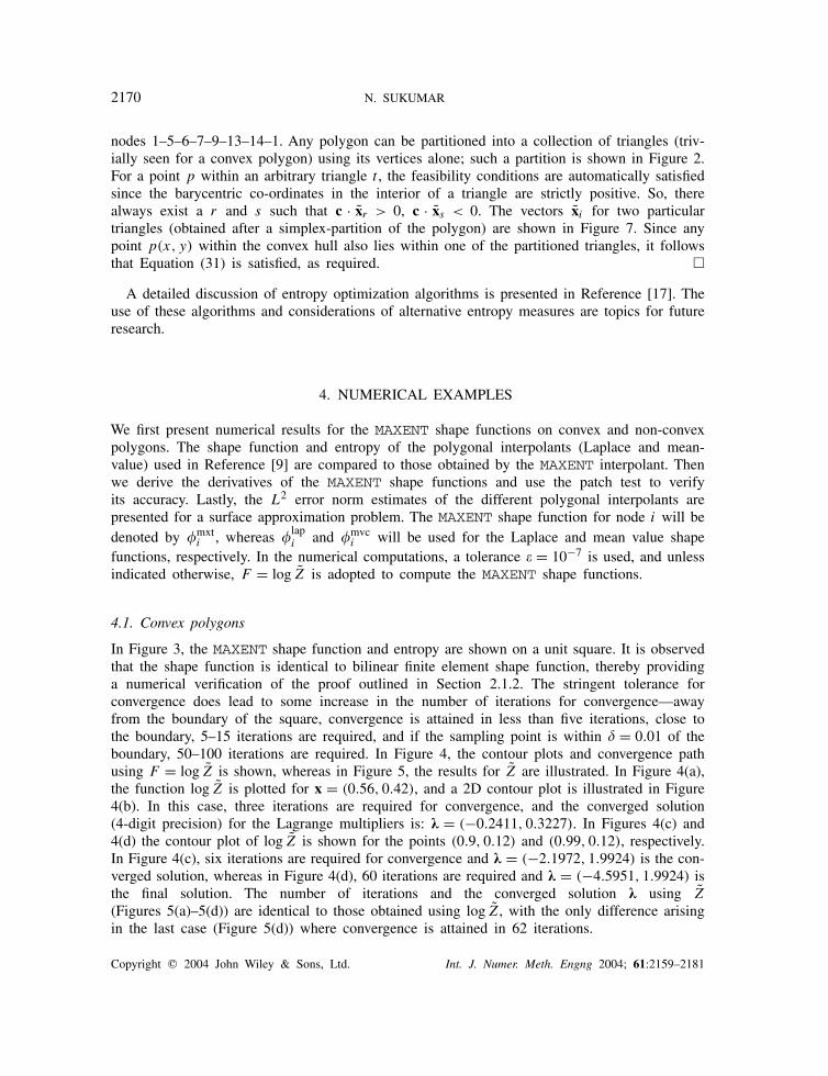
4.1. Convex polygons

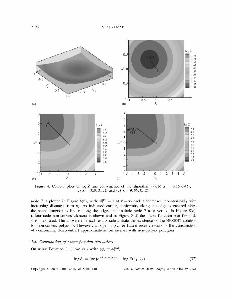
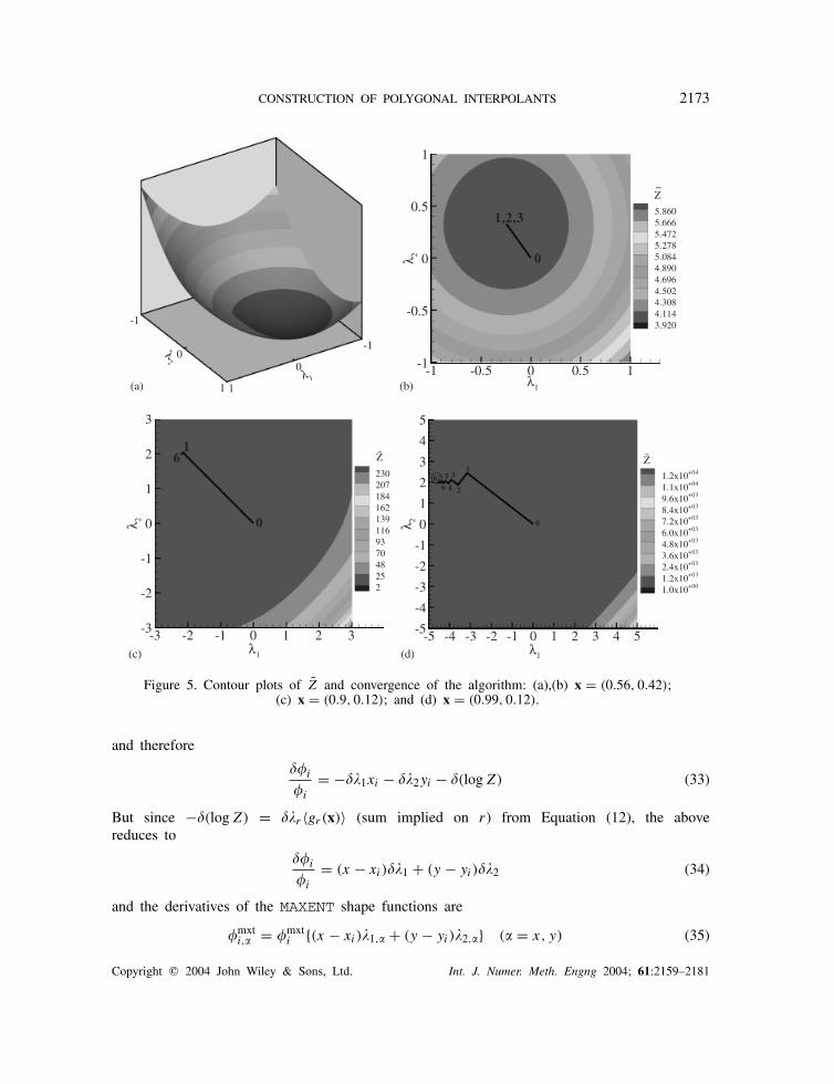
In Figure 3, the MAXENT shape function and entropy are shown on a unit square. It is observedthat the shape function is identical to bilinear finite element shape function, thereby providinga numerical verification of the proof outlined in Section 2.1.2. The stringent tolerance forconvergence does lead to some increase in the number of iterations for convergence—awayfrom the boundary of the square, convergence is attained in less than five iterations, close tothe boundary, 5–15 iterations are required, and if the sampling point is within = 0.01 of theboundary, 50–100 iterations are required. In Figure 4, the contour plots and convergence pathusing F = log Z is shown, whereas in Figure 5, the results for Z are illustrated. In Figure 4(a),the function log Z is plotted for x = (0.56, 0.42), and a 2D contour plot is illustrated in Figure4(b). In this case, three iterations are required for convergence, and the converged solution(4-digit precision) for the Lagrange multipliers is: = (−0.2411, 0.3227). In Figures 4(c) and4(d) the contour plot of log Z is shown for the points (0.9, 0.12) and (0.99, 0.12), respectively.In Figure 4(c), six iterations are required for convergence and = (−2.1972, 1.9924) is the con-verged solution, whereas in Figure 4(d), 60 iterations are required and = (−4.5951, 1.9924) isthe final solution. The number of iterations and the converged solution using Z

(Figures 5(a)–5(d)) are identical to those obtained using log Z, with the only difference arisingin the last case (Figure 5(d)) where convergence is attained in 62 iterations.



X

0

0.5

1

Y

0

0.5

1

φ

0

0.5

1

ENTROPY

1.31.21.110.90.80.70.60.50.40.30.20.10

(a) (b)

Figure 3. Numerical computations using the MAXENT formulation on a unit square.(a) shape function; and (b) entropy.

In Figures 6(a)–6(c), the MAXENT, Laplace, and mean-value shape functions for node 1 ina regular hexagon are shown. The plots for the Laplace and MAXENT shape functions aresimilar, whereas mvc

1 is distinct. To further reveal the relationship between these interpolants,we plotted the ratio of the entropy of the Laplace and mean value shape functions to thatobtained (maximum entropy) using the MAXENT shape functions. These results are presented inFigures 6(d) and 6(e). It is clearly observed that using the entropy as a measure, the Laplaceinterpolant is proximal to the MAXENT interpolant.

4.2. Non-convex polygons

We had earlier proved that the MAXENT formulation leads to a feasible solution for the shapefunctions on non-convex polygons. Referring once again to the n-gon shown in Figure 2, wenow conduct numerical computations in support of the proof. In Figures 7(a) and 7(b), weshow the shape function variation of node 6 (mxt

6 ) and the maximum entropy distributionfor the case when the shape functions are assumed to be known along the boundary of theconvex hull, ch. In this case, nodal interpolation is not realized at nodes that are locatedin the interior of the convex hull. In Figures 7(c) and 7(d), the plots are depicted for thecase when the shape functions are known along e. We note that the variation of mxt

6 usingeither approach is very similar, with some difference arising along the edges that do not includenode 6. The latter case is presented since even though it involves a modification to the maximumentropy distribution, it would lead to inter-element continuity; however continuity inside theelement and close to the edge would not be rigorously met. The maximum value of the entropy(log 15) is attained at the centroid.

We present shape functions on two meshes that contain non-convex elements. In bothexamples, we assume linear interpolation along the boundary e. In Figure 8(a), thedomain is a bi-unit square and node 7 is located at (0.4, 0). The MAXENT shape function for


2172 N. SUKUMAR

λ1

-1

-0.5

0

0.5

1

λ 2

-1-0.5

00.5

1

~

1,2,3

log Z

0

λ1

λ 2

-1 -0.5 0 0.5 1-1

-0.5

0

0.5

1

1.761.721.681.651.611.571.531.491.461.421.38

~1

6

0

log Z

λ1

λ 2

-3 -2 -1 0 1 2 3-3

-2

-1

0

1

2

3

5.705.174.644.113.583.052.521.991.460.930.40

log Z~

2

34

56

601

0

λ1

λ 2

-5 -4 -3 -2 -1 0 1 2 3 4 5-5

-4

-3

-2

-1

0

1

2

3

4

5

9.48.57.66.75.84.94.03.12.21.30.4

(a) (b)

(c) (d)

Figure 4. Contour plots of log Z and convergence of the algorithm: (a),(b) x = (0.56, 0.42);(c) x = (0.9, 0.12); and (d) x = (0.99, 0.12).

node 7 is plotted in Figure 8(b), with mxt7 = 1 at x = x7 and it decreases monotonically with

increasing distance from x7. As indicated earlier, conformity along the edge is ensured sincethe shape function is linear along the edges that include node 7 as a vertex. In Figure 8(c),a four-node non-convex element is shown and in Figure 8(d) the shape function plot for node4 is illustrated. The above numerical results substantiate the existence of the MAXENT solutionfor non-convex polygons. However, an open topic for future research-work is the constructionof conforming (barycentric) approximations on meshes with non-convex polygons.

4.3. Computation of shape function derivatives

On using Equation (11), we can write (i ≡ mxti )

log i = log(e−1xi−2yi

) − log Z(1, 2) (32)



λ1

-1

0

1

λ2

-1

0

1

~

1,2,3

0

Z

λ1

λ 2

-1 -0.5 0 0.5 1-1

-0.5

0

0.5

1

5.8605.6665.4725.2785.0844.8904.6964.5024.3084.1143.920

0

1 ~6 Z

λ1

λ 2

-3 -2 -1 0 1 2 3-3

-2

-1

0

1

2

3

230207184162139116937048252

0

1

2

3

45

6

~Z

62

λ1

λ 2

-5 -4 -3 -2 -1 0 1 2 3 4 5-5

-4

-3

-2

-1

0

1

2

3

4

5

1.2x10+04

1.1x10+04

9.6x10+03

8.4x10+03

7.2x10+03

6.0x10+03

4.8x10+03

3.6x10+03

2.4x10+03

1.2x10+03

1.0x10+00

(a) (b)

(c) (d)

Figure 5. Contour plots of Z and convergence of the algorithm: (a),(b) x = (0.56, 0.42);(c) x = (0.9, 0.12); and (d) x = (0.99, 0.12).

and therefore

i

i

= −1xi − 2yi − (log Z) (33)

But since −(log Z) = r〈gr(x)〉 (sum implied on r) from Equation (12), the abovereduces to

i

i

= (x − xi)1 + (y − yi)2 (34)

and the derivatives of the MAXENT shape functions are

mxti, = mxt

i (x − xi)1, + (y − yi)2, ( = x, y) (35)


2174 N. SUKUMAR

φ1mxt

10.90.80.70.60.50.40.30.20.10

1

φ1lap

10.90.80.70.60.50.40.30.20.10

1

φ1mvc

10.90.80.70.60.50.40.30.20.10

1

H/H

10.99850.9970.99550.9940.99250.9910.98950.9880.98650.985

(a) (b)

(c) (d)

(e)

H/Hmax

max

10.990.980.970.960.950.940.930.920.910.9

Figure 6. Shape function and entropy plots on a regular hexagon: (a) mxt1 ; (b) lap

1 ; (c) mvc1 ;

(d) H(lapi )/Hmax; and (e) H(mvc

i )/Hmax.

where (·),x = (·)/x and (·),y = (·)/y. Now, we need to determine r,x ≡ r/〈g1(x)〉and r,y ≡ r/〈g2(x)〉. To this end, we once again consider Equation (12)

−(log Z)

r

= 〈gr(x)〉 (r = 1, 2) (36)



X

Y

0 0.5 1 1.5 20

0.5

1

1.5

φ6

10.90.80.70.60.50.40.30.20.10

6

Hmod

2.62.42.221.81.61.41.210.80.60.40.2

(a) (b)

(d)(c)

X

Y

0 0.5 1 1.5 20

0.5

1

1.5

φ6

10.90.80.70.60.50.40.30.20.10

6

Hmax

2.62.42.221.81.61.41.210.80.60.40.2

Figure 7. MAXENT solution in a non-convex polygon. Shape function mxt6 and distribution of entropy

assuming: (a) and (b) interpolation along ch; and (c) and (d) interpolation along e.

and on taking the derivative of the above equation with respect to s , we obtain

〈gr(x)〉s

= 〈gs(x)〉r

= −2(log Z)

rs

≡ − 2F

rs

= −Grs (37)

where for notational convenience we have used F = log Z (earlier F was set to log Z) and Gis the Hessian of log Z(1, 2). On using the chain rule of differentiation, we can write

r

〈gs(x)〉 = −[G−1]rs (38)


2176 N. SUKUMAR

7

X

-1

-0.5

0

0.5

1

Y

-1

-0.5

0

0.5

1

4

4

(a) (b)

(d)(c)

Figure 8. Modified MAXENT shape function in a non-convex polygonal mesh: (a) seven-node mesh;(b) mxt

7 ; (c) four-node mesh; and (d) mxt4 .

and since 〈g1(x)〉 = x and 〈g2(x)〉 = y, we obtain

1

x

1

y

2

x

2

y

= −

[G11 G12

G21 G22

]−1

(39)

Since F(1, 2) = log Z(1, 2) = log(∑n

i e−1xi−2yi

), we can write its derivative with respect

to 1 as:

F

1=

∑ni=1 e−1xi−2yi (−xi)

Z(40)



or

G11 = 2F

21

=Z∑n

i=1 e−1xi−2yi x2i +

[∑ni=1 e−1xi−2yi (xi)

] [∑ni=1 e−1xi−2yi (−xi)

]Z2 (41)

which simplifies to

G11 =∑n

i=1 e−1xi−2yi x2i

Z− x2 (42)

and therefore

G11 =n∑

i=1mxt

i x2i − x2 ≡ 〈x2〉 − x2 (variance of x) (43)

Proceeding likewise for the other components of G, we have

G12 = G21 = 〈xy〉 − xy, G22 = 〈y2〉 − xy (44)

Now we can write Equation (39) as

1

x

1

y

2

x

2

y

= −

[ 〈x2〉 − x2 〈xy〉 − xy

〈xy〉 − xy 〈y2〉 − y2

]−1

(45)

and on using the above relations in Equation (35), the derivatives of the MAXENT shapefunctions are computed.

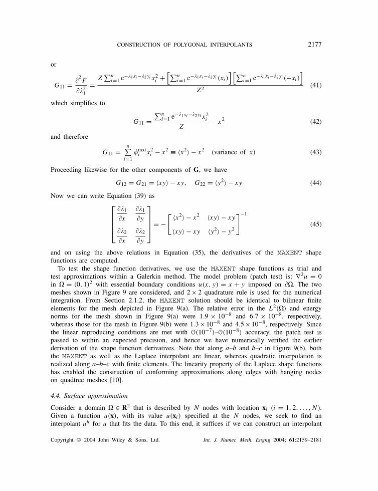
To test the shape function derivatives, we use the MAXENT shape functions as trial andtest approximations within a Galerkin method. The model problem (patch test) is: ∇2u = 0in = (0, 1)2 with essential boundary conditions u(x, y) = x + y imposed on . The twomeshes shown in Figure 9 are considered, and 2 × 2 quadrature rule is used for the numericalintegration. From Section 2.1.2, the MAXENT solution should be identical to bilinear finiteelements for the mesh depicted in Figure 9(a). The relative error in the L2() and energynorms for the mesh shown in Figure 9(a) were 1.9 × 10−8 and 6.7 × 10−8, respectively,whereas those for the mesh in Figure 9(b) were 1.3 × 10−8 and 4.5 × 10−8, respectively. Sincethe linear reproducing conditions are met with O(10−7)–O(10−8) accuracy, the patch test ispassed to within an expected precision, and hence we have numerically verified the earlierderivation of the shape function derivatives. Note that along a–b and b–c in Figure 9(b), boththe MAXENT as well as the Laplace interpolant are linear, whereas quadratic interpolation isrealized along a–b–c with finite elements. The linearity property of the Laplace shape functionshas enabled the construction of conforming approximations along edges with hanging nodeson quadtree meshes [10].4.4. Surface approximation

Consider a domain ∈ R2 that is described by N nodes with location xi (i = 1, 2, . . . , N).Given a function u(x), with its value u(xi ) specified at the N nodes, we seek to find aninterpolant uh for u that fits the data. To this end, it suffices if we can construct an interpolant


2178 N. SUKUMAR

a

c

b

(a) (b)

Figure 9. Meshes for the patch test: (a) regular; and (b) edge with three nodes.

within each polygon Vi , where = ∪Vi , and the global interpolant is then the additive sumof the local interpolant on each polygon. From approximation theory, we know that givenindependent elements xini=1 with aixi ∈ X (X is a normed linear space), then the bestapproximation to an element y ∈ X is determined by minai

‖y − ∑ni=1 aixi‖, i.e. the weights

ai are obtained by minimizing the L2 norm of the error [18].If one considers the interpolation of random fields, then the above notion of best-approxi-

mation also applies to the MAXENT interpolant. Let u be the approximation for u that minimizesthe square of the expected error. Then, on using the MAXENT shape function in Equation (2),we have

〈(u − u)2〉 =n∑

i=1mxt

i (ui − u)2 (46)

or

〈(u − u)2〉 = 〈u2〉 − 2u〈u〉 + u2 (47)

and on adding and subtracting 〈u〉2 to the right-hand side, we obtain

〈(u − u)2〉 = 〈u2〉 − 〈u〉2︸︷︷︸variance of u

+(u − 〈u〉)2 (48)

and since the variance of u is a fixed quantity, the expected error is minimized if u = 〈u〉,and therefore

u(x) = uh(x) =n∑

i=1mxt

i ui (49)

is the least-biased interpolant with respect to the location of the nodal co-ordinates xi and italso minimizes the mean-square expected error [2].



X

Y

0 0.2 0.4 0.6 0.8 10

0.2

0.4

0.6

0.8

1

|u - uh|0.0160.0140.0120.0110.0090.0070.0050.0040.0020.000

X

Y

0 0.2 0.4 0.6 0.8 10

0.2

0.4

0.6

0.8

1

|u - uh|0.0160.0140.0120.0110.0090.0070.0050.0040.0020.000

X

Y

0 0.2 0.4 0.6 0.8 10

0.2

0.4

0.6

0.8

1

|u - uh|0.0160.0140.0120.0110.0090.0070.0050.0040.0020.000

(a) (b)

(c)

Figure 10. Point-wise absolute error for the interpolation of u(x, y) = x2+y2: (a) MAXENT; (b) Laplace;and (c) mean-value interpolants.

We consider the problem of data interpolation to examine the accuracy of the MAXENTinterpolant vis-à-vis some of the other polygonal interpolants. In the examples that follow, thequadratic function u(x) = x2 + y2 is interpolated within the domain = (0, 1)2. To constructa mesh, the seed points that define the Voronoi diagram were inserted using a random numbergenerator that was based on a uniform probability distribution in (0, 1) [16]. If m points areinserted, a Voronoi mesh with m elements is obtained; the vertices of the Voronoi cells are thenodes. For comparison purposes, we measure the absolute accuracy using the discrete L2()

norm, where ‖u − uh‖2L2 = ∑M

i=1(u(xi )−uh(xi ))2 and M is the total number of points chosen

in the domain. The maximum error norm maxi |u(xi ) − uh(xi )|∞ is also computed. Points thatare located on e are not used in the computations since the interpolants under considerationare identical along e. In Figure 10, the point-wise absolute error is presented for the MAXENT,Laplace, and mean-value interpolants; the mesh consists of 100 elements (202 nodes). Eachn-gon is partitioned into 16n triangles, and the interpolant is evaluated at the vertices of thesetriangles. The discrete L2 (L∞) error norms that were obtained are: 0.4486 (1.556 × 10−2),0.4457 (1.559 × 10−2), and 0.4124 (1.562 × 10−2), respectively. The above trends were also


2180 N. SUKUMAR

X

Y

0.2 0.4 0.6 0.8 10

0.2

0.4

0.6

0.8

1

|u - uh|0.170.148750.12750.106250.0850.063750.04250.021250

Figure 11. Point-wise absolute error for the modified MAXENT interpolant on a meshcontaining non-convex elements.

consistent on other meshes that we considered. From the contour plots shown in Figure 10,the close correspondence between the results for the Laplace and MAXENT interpolants is onceagain noted.

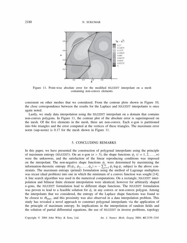
Lastly, we study data interpolation using the MAXENT interpolant on a domain that containsnon-convex polygons. In Figure 11, the contour plot of the absolute error is superimposed onthe mesh. Of the five elements in the mesh, three are non-convex. Each n-gon is partitionedinto 64n triangles and the error computed at the vertices of these triangles. The maximum errornorm (sup-norm) is 0.17 for the mesh shown in Figure 11.

5. CONCLUDING REMARKS

In this paper, we have presented the construction of polygonal interpolants using the principleof maximum entropy (MAXENT). On an n-gon (n > 3), the shape functions i (i = 1, 2, . . . , n)were the unknowns, and the satisfaction of the linear reproducing conditions was imposedon the interpolant. The non-negative shape functions i were determined by maximizing theinformation-theoretic entropy H(1, 2, . . . , n) = −∑n

i=1 i log i subject to the above con-straints. The maximum entropy (primal) formulation using the method of Lagrange multiplierswas recast (dual problem) into one in which the minimum of a convex function was sought [14].A line search algorithm was used in the numerical computations. On a rectangle, MAXENT inter-polation and bilinear finite element interpolation were identical; however for arbitrarily shapedn-gons, the MAXENT formulation lead to different shape functions. The MAXENT formulationwas proven to lead to a feasible solution for i in any convex or non-convex polygon. Amongthe interpolants that we considered, the entropy of the Laplace shape functions was found tobe closest to Hmax, and this proximity was also observed in a data interpolation problem. Thisstudy has revealed a novel approach to construct polygonal interpolants via the application ofthe principle of maximum entropy. Its implications in the interpolation of random fields andthe solution of partial differential equations, the use of MAXENT in inverse problems, topology



optimization and material design, and the natural link towards the development of multiscalenumerical methods are deemed to be noteworthy.

ACKNOWLEDGEMENTS

The author is grateful for the research support of the National Science Foundation through contractCMS–0352654 to the University of California, Davis. It is a pleasure to also acknowledge ProfessorYueyue Fan for many helpful discussions on constrained optimization and generalized inverse.

REFERENCES

1. Shannon CE. A mathematical theory of communication. The Bell Systems Technical Journal 1948; 27:379–423.2. Jaynes ET. Information theory and statistical mechanics. Physical Review 1957; 106(4):620–630.3. Jaynes ET. Information theory and statistical mechanics. II. Physical Review 1957; 108(2):171–190.4. Jaynes ET. On the rationale of maximum-entropy methods. Proceedings of the IEEE 1982; 70(9):939–952.5. Rosenkrantz RD. (ed.). E.T. Jaynes, Paper on Probability, Statistics and Statistical Physics. Kluwer Academic

Publishers: Dordrecht, The Netherlands, 1989.6. Khinchin A. Mathematical Foundations of Information Theory. Dover: New York, NY, 1957.7. Kapur JN. Maximum-Entropy Models in Science and Engineering (1st (revised) edn). Wiley: New Delhi,

India, 1993.8. Beltzer AI. Entropy characterization of finite elements. International Journal of Solids and Structures 1996;

33(24):3549–3560.9. Sukumar N, Tabarraei A. Conforming polygonal finite elements. International Journal for Numerical Methods

in Engineering 2004; 61:2045–2066.10. Tabarraei A, Sukumar N. Adaptive computations on conforming quadtree meshes. Finite Elements in Analysis

and Design, 2005, to appear (Special Issue on Papers Presented at the Robert J. Melosh Finite ElementMedal Competition.)

11. Jaynes ET. Concentration of distributions at entropy maxima. In E.T. Jaynes, Paper on Probability, Statisticsand Statistical Physics, Rosenkrantz RD (ed.). Kluwer Academic Publishers: Dordrecht, The Netherlands,1989; 317–336.

12. Penrose R. A generalized inverse for matrices. Proceedings of the Cambridge Philosophical Society 1955;51:406–413.

13. Agmon N, Alhassid Y, Levine RD. An algorithm for determining the Lagrange parameters in the maximalentropy formalism. In The Maximum Entropy Formalism, Tribus M, Levine RD (eds). MIT Press: Cambridge,MA, 1978; 206–209.

14. Agmon N, Alhassid Y, Levine RD. An algorithm for finding the distribution of maximal entropy. Journalof Computational Physics 1979; 30:250–258.

15. Alhassid Y, Agmon N, Levine RD. An upper bound for the entropy and its application to the maximalentropy problem. Chemical Physics Letters 1978; 53(1):22–26.

16. Press WH, Flannery BP, Teukolsky SA, Vetterling WT. Numerical Recipes in Fortran: The Art of ScientificComputing (2nd edn). Cambridge University Press: New York, NY, 1992.

17. Fang S-C, Rajasekera JR, Tsao HSJ. Entropy Optimization and Mathematical Programming. Kluwer AcademicPublishers: Dordrecht, The Netherlands, 1997.

18. Davis PJ. Interpolation and Approximation. Dover: New York, NY, 1975.


construction of polygonal interpolants: a maximum entropy...

Documents