construction of low dissipative high-order well-balanced filter schemes for non-equilibrium flows

Construction of Low Dissipative High-Order Well-Balanced

Filter Schemes for Non-Equilibrium Flows

Wei Wang∗, H. C. Yee†, Bjorn Sjogreen‡, Thierry Magin∗, and Chi-Wang Shu§

December 6, 2009

Abstract

The goal of this paper is to generalize the well-balanced approach for non-equilibriumflow studied by Wang et al. [27] to a class of low dissipative High-order shock-capturingfilter schemes and to explore more advantages of well-balanced schemes in reacting flows.More general 1D and 2D reacting flow models and new examples of shock turbulence in-teractions are provided to demonstrate the advantage of well-balanced schemes. The classof filter schemes developed by Yee et al. [31], Sjogreen & Yee [25] and Yee & Sjogreen [36]consist of two steps, a full time step of spatially high-order non-dissipative base schemeand an adaptive nonlinear filter containing shock-capturing dissipation. A good propertyof the filter scheme is that the base scheme and the filter are stand alone modules in de-signing. Therefore, the idea of designing a well-balanced filter scheme is straightforward,i.e., choosing a well-balanced base scheme with a well-balanced filter (both with high-orderaccuracy). A typical class of these schemes shown in this paper is the high-order central dif-ference schemes/predictor-corrector (PC) schemes with a high-order well-balanced WENOfilter. The new filter scheme with the well-balanced property will gather the featuresof both filter methods and well-balanced properties: it can preserve certain steady-statesolutions exactly; it is able to capture small perturbations, e.g., turbulence fluctuations;and it adaptively controls numerical dissipation. Thus it shows high accuracy, efficiencyand stability in shock/turbulence interactions. Numerical examples containing 1D and 2Dsmooth problems, 1D stationary contact discontinuity problem and 1D turbulence/shockinteractions are included to verify the improved accuracy, in addition to the well-balancedbehavior.

Key words: High-order filter methods, WENO schemes, well-balanced schemes, non-equilibrium flow, chemical reactions, 1D turbulence/shock interactions.

1 Introduction

Recent progress in the development of a class of low dissipative high-order filter schemes formultiscale Navier-Stokes and magnetohydrodynamics (MHD) systems [31, 38, 25, 33, 24, 34,35, 36] shows good performance in multiscale shock/turbulence simulations.

∗Center for Turbulence Research, Stanford University, Stanford, CA 94305†NASA Ames Research Center, Moffett Field, CA 94035‡Lawrence Livermore National Laboratory, Livermore, CA 94551§Division of Applied Mathematics, Brown University, Providence, RI 02912

1

The highly parallelizable high-order filter methods consist of two steps, a full time stepof spatially high-order non-dissipative (or very low dissipative) base scheme and an adaptivemultistep filter. The nonlinear filter consists of the product of a wavelet-based flow sensor andthe dissipative portion of a high-order shock-capturing scheme. The built-in flow sensors inthe post processing filter control the amounts and types of numerical dissipation. The filterswitches on the dissipations only where needed, and leaves the rest of the flow region freefrom numerical dissipation. Only the filter step might involve the use of flux limiters andapproximate Riemann solvers as stabilizing mechanisms to remove Gibbs phenomena relatedspurious oscillations resulting from the base scheme step. The more scales that are resolvedby the base scheme, the less the filter is utilized, thereby gaining accuracy and computationaltime as the grid is refined. The adaptive numerical dissipation control idea is very generaland can be used in conjunction with spectral, spectral element, finite element, discontinuousGalerkin, finite volume, and finite difference spatial base schemes. The type of shock-capturingschemes used as nonlinear dissipation can be the dissipative portion of any high resolution TVD,MUSCL, ENO, or WENO shock-capturing method [31, 11, 21]. By design, flow sensors, spatialbase schemes and linear and nonlinear dissipation models are stand alone modules. Therefore,a whole class of low dissipative high-order schemes can be derived at ease.

In a recent paper by Wang et al. [27], well-balanced finite difference WENO schemes andsecond-order TVD schemes were studied for chemical non-equilibrium flows, extending thewell-balanced finite difference WENO schemes for shallow water equations in [28, 29]. A well-balanced scheme [13], which can preserve certain nontrivial steady-state solutions exactly, mayhelp minimize some of the spurious oscillations around steady states. It was also shown in [27]that the well-balanced schemes capture small perturbations of the steady-state solutions withhigh accuracy. While general schemes can only resolve perturbations at the level of truncationerror with the specific grid, well-balanced schemes can resolve much smaller perturbations,usually of size 1% or lower of the main steady-state flow.

In this paper the same approach will be applied to construct a high-order well-balanced filterscheme for one temperature non-equilibrium flow with reaction terms. The multi-dimensionalhyperbolic system of conservation laws with source terms (also called a balance law)

Ut + ∇ · F (U) = S(U) (1)

is considered, where U is the solution vector, F (U) is the convective flux and S(U) is thesource term. For this type of flow the space variable x does not appear explicitly in the sourceterm. Thus, the construction of well-balanced schemes can easily go from one-dimension tomulti-dimensions. In this paper, comparing with our earlier work [27], more general 1D and2D reacting flow models and new examples of shock turbulence interactions are provided todemonstrate the advantage of well-balanced schemes.

The designing of well-balanced filter schemes is to choose a well-balanced base scheme anda well-balanced filter part. Then, the filter scheme is almost well-balanced everywhere exceptat the interfaces of the filtered region and the non-filtered region (see Sec. 5). Note that in thisarticle, a ‘well-balanced filter scheme’ refers to such almost well-balancedness. For the filterscheme without the flow sensor, the resulting filter scheme is well-balanced.

The choice of the sensor will not destroy the well-balanced properties. It has been shown inthe previous work [27] that linear schemes, the second-order Predictor-Corrector (PC) scheme[32, 14] with TVD filters (such as the Harten-Yee TVD filter [30, 31]), and WENO-Roe schemes

2

are well-balanced for certain steady-state solutions with zero velocity. A well-balanced WENO-LF scheme has also been constructed for this type of steady-state solutions. High-order PCschemes are linear schemes and thus well-balanced. Therefore, the new filter schemes presentedin this article, CENTVDfi/CENWENOfi or PCTVDfi/PCWENOfi which utilize central/PCschemes as base schemes and the Harten-Yee TVD filter or the well-balanced WENO schemesas filter will be well-balanced.

In this paper, only the zero-velocity steady state of the reacting flow equations will beconsidered in the numerical tests. A steady state with zero velocity implies that the flow hasconstant pressure and is in chemical equilibrium. It will be shown that, similarly to well-balanced WENO schemes, well-balanced filter schemes give machine round-off errors regardlessof the mesh sizes for the steady-state solutions of the reactive flow equations. Consequently,they can resolve small perturbations of such steady state solutions well, even with very coarsemeshes.

Since the regular high-order low dissipative filter schemes are designed for shock/turbulenceinteractions and the well-balanced schemes can capture small perturbations of the steady statesolutions with high accuracy, the new well-balanced filter schemes take the advantages of both,thereby making them well suited for computations of turbulent fluctuations on a mainly steadyflow field.

The outline of the paper is at follows: in Sec. 2, the governing equations and the physicalmodel are described. High-order filter schemes and well-balanced schemes are reviewed in Secs. 3and 4. The proposed high-order well-balanced filter scheme is introduced in Sec. 5. Numericalexamples will be shown in Sec. 6. Finally, Sec. 7 gives conclusions and plans for future work. Abrief description of high order PC schemes and the considered time discretization are presentedin the Appendix.

2 Governing equations and physical model

Considering a flow in chemical nonequilibrium and thermal equilibrium, the thermodynamicproperties account for excitation of the electronic states for the atoms and molecules, andno vibrational states based on the rigid-rotor harmonic-oscillator approximation for molecules[15, 18].

Assuming neither dissipative effects nor radiation, the considered physical model is a systemof hyperbolic conservation laws with source terms denoted by

Ut + ∇ · F (U) = S(U), (2)

U =

ρ1

. . .ρns

ρuρe

; F (U) =

ρ1u. . .ρns

uρuuT + pI(ρe+ p)u

; S(U) =

b1. . .bns

00

; (3)

where ns is the number of species, ρs, the mass density of species s, u, the velocity vector, ande, the internal energy per unit mass of the mixture. The mixture mass density is defined as

3

ρ =∑ns

s=1 ρs, and the pressure p is given by the perfect gas law

p = RT

ns∑

s=1

ρs

Ms, (4)

where R is the universal gas constant, and Ms, the molar mass of species s. The temperatureT can be found from a given total energy by solving

ρe =

ns∑

s=1

ρses(T ) +1

2ρ|u|2, (5)

for T . The internal energy es of species s is a function of temperature

es(T ) = eTs (T ) + eE

s (T ) + eFs , s ∈ Ha, (6)

es(T ) = eTs (T ) + eE

s (T ) + eRs (T ) + eV

s (T ) + eFs , s ∈ Hp, (7)

where Ha is the set of atoms and Hp is the set of molecules. The superscripts “T” denotestranslation, “E” denotes electron, “R” denotes Rotation, “V” denotes vibration and “F” denotesformation. The translational energy of species s is given by

eTs (T ) =

3

2

R

MsT, (8)

and the electronic energy contribution by

eEs (T ) =

R

Ms

∑

ngEs,nθ

Es,n exp

(

−θEs,n

T

)

∑

ngEs,n exp

(

−θEs,n

T

) , (9)

where quantities gEs,n and θE

s,n stand for the degeneracy and characteristic temperature of theelectronic level n of species s. Only a finite number of electronic states is retained in thecomputation of partition function. The maximum number of electronic levels of each atomand molecule is progressively increased up to a correspondence between the values of computedenthalpies and accurate reference tables. For molecule s, the rotational energy is assumed tobe described by means of a rigid rotor model

eRs (T ) =

RT

Ms, (10)

and the vibrational energy, by means of a harmonic oscillator model

eVs (T ) =

R

Ms

θVs

exp(

θVs

T

)

− 1, (11)

where the quantity θVs stands for the vibrational characteristic temperature of the diatomic

molecule. To account for the energy released in the gas by chemical reactions between the

4

species, a common level from which all the energies are measured is established by using theformation enthalpy eF

s at 0K.The source term S(U) describes the chemical reactions occurring in gas flows which result

in changes in the amount of mass of each chemical species. In the general case there are Jreactions of the form

ν′1,jX1 + ν′2,jX2 + · · · + ν′ns,jXns ν′′1,jX1 + ν′′2,jX2 + · · · + ν′′ns,jXns

, j = 1, . . . , J, (12)

where ν′i,j and ν′′i,j are respectively the stoichiometric coefficients for the reactants and productsof species i in the jth reaction. For non-equilibrium chemistry the rate of production of speciesi due to chemical reaction may be written as

bi = Mi

J∑

j=1

(ν′′i,j − ν′i,j)

[

kf,j

ns∏

s=1

(

ρs

Ms

)ν′

s,j

− kb,j

ns∏

s=1

(

ρs

Ms

)ν′′

s,j

]

, i = 1, . . . , ns. (13)

For each reaction j the forward and backward reaction rate coefficients, kf,j and kb,j are assumedto be known functions of temperature. The forward reaction rate coefficient is given by anArrhenius law. Following microreversibity the backward rate coefficient is obtained from theexpression kf,j = kb,j/Ke,j , where the equilibrium constant for the jth reaction is given by therelation

lnKe,j = −1

kBT

ns∑

s=1

[(ν′′s,j − ν′s,j)msgs(pref , T )], (14)

where the reference pressure pref = 1 Pa. The Gibbs free energy gs of species s is a functionof pressure and temperature,

gs(p, T ) = gTs (p, T ) + gE

s (T ), s ∈ Ha, (15)

gs(p, T ) = gTs (p, T ) + gE

s (T ) + gRs (T ) + gV

s (T ), s ∈ Hp. (16)

The translational Gibbs free energy is obtained from

gTs (p, T ) =

RT

Msln

[

RT

NAp

(

2πMsRT

N2Ah

2P

)32

]

, (17)

where the symbol hP stands for Planck’s constant, and NA for Avogadro’s number. Theelectronic Gibbs free energy reads

gEs (T ) = −

RT

Msln

[

∑

n

gEs,n exp

(

−θEs,n

T

)]

. (18)

For the diatomic molecule s, the rotational Gibbs free energy is

gRs (T ) = −

RT

Msln

(

T

θRs σs

)

, (19)

where symbol σs stands for the steric factor. The vibrational Gibbs free energy is obtainedfrom the relation

gVs (T ) =

RT

Msln

[

1 − exp

(

−θVs

T

)]

. (20)

5

3 Description of high-order filter methods

For simplicity of presentation, the numerical methods will be described for the one-dimensionalequations. In one space dimension F in Eq. (3) becomes a vector. Denote A = ∂F/∂U , theJacobian matrix of the one dimensional flux. The eigenvalues of A are

(a1, . . . , am) = (u, . . . , u, u+ c, u− c), (21)

where m is the number of components of vector U , m = ns + 2 in the 1D case. c is the frozenspeed of sound defined by the expression c2 = (κ+1)p/ρwith κ = (

∑ns

s=1 ρsR/Ms)/(∑ns

s=1 ρscv,s)based on the species specific heat cv,s = des/dT .

The one dimensional problem is discretized by a uniform grid spacing ∆x and the gridpoints xj = j∆x. The time step is denoted by ∆t and time levels are tn = n∆t. Let Un

j denotethe numerical approximation of U(xj , tn). For clarity of presentation, the n- or j-dependenciesare left out when they are unimportant in the discussion below.

Let alj+1/2, and Rj+1/2 denote the eigenvalues al and the eigenvectors R evaluated at some

symmetric average of Uj and Uj+1, such as Roe’s average [22]. Denote R as the matrix whosecolumns are eigenvectors of A (not to be confused with the R in Eq. (4)). Define

αj+1/2 = R−1j+1/2(Uj+1 − Uj) (22)

as the difference of the local characteristic variables in the x direction.The low dissipative high-order filter scheme developed by Yee et al. [31] suggests using the

artificial compression method of Harten [7] as a flow sensor to limit the amount of numericaldissipation that is inherent in a scheme. Subsequently, Sjogreen and Yee [25], Yee and Sjogreen[34, 36] introduced a wavelet decomposition of the data to determine the location where numer-ical dissipation is needed. The considered filter method contains two steps, a high-order lowdissipative spatial base scheme step (not involving the use of approximate Riemann solvers orflux limiters) and a multistep filter (usually involving the use of approximate Riemann solversand flux limiters). The nonlinear filter consists of the product of a wavelet sensor [25] and thenonlinear dissipative portion of a high-resolution shock-capturing scheme.

We will briefly review the high-order filter schemes in this section. For more details, werefer the readers to [31, 25, 34, 36].

3.1 High-order spatial scheme step

The first step of the numerical method consists of a time step via a high-order non-dissipativespatial and high-order temporal base scheme operator L. After the completion of a full timestep of the base scheme, the solution is denoted by U ∗

U∗ = L(Un), (23)

where Un is the numerical solution vector at time level n.The high-order non-dissipative spatial base scheme could be a standard central scheme, a

central compact scheme, or a predictor-corrector (PC) scheme [32, 14].For strong shock interactions and/or steep gradient flows, a small amount of high-order

linear dissipation can be added to the base scheme to reduce the time step constraint and

6

stability. For example, an eighth-order linear dissipation with the sixth-order central schemeto approximate F (U)x is written as

∂F

∂x|x=xj

≈ D06 Fj + d(∆x)7(D+D−)4Uj , (24)

where D06 is the standard sixth-order accurate centered difference operator, and D+D− is thestandard second-order accurate centered approximation of the second derivative. The smallparameter d is scaled with, e.g., spectral radius of A(U), and is in the range of 0.00001-0.001,depending on the flow problem. d has the sign which gives dissipation in the forward timedirection.

In Section 6, we will use high-order central schemes and PC schemes for the base scheme step.Details on these methods, and other choices of spatial base schemes, are given in Appendix A.

3.2 Adaptive nonlinear filter step (discontinuities and high gradientcapturing)

After the completion of a full time step of the high-order base scheme, the second step is toadaptively filter the solution by the product of a wavelet sensor and the nonlinear dissipativeportion of a high-resolution shock-capturing scheme (involving the use of flux limiters). Thenonlinear filter step can be written

Un+1j = U∗

j −∆t

∆x

[

H∗j+1/2 −H∗

j−1/2

]

. (25)

Here, the filter numerical fluxes are defined in the eigenvector basis by Hj+1/2, so that

H∗j+1/2 = Rj+1/2Hj+1/2. (26)

Denote the elements of the vector Hj+1/2 by hlj+1/2, l = 1, 2, . . .m. The nonlinear portion of

the filter hlj+1/2 has the form

hlj+1/2 = (sN )l

j+1/2(φlj+1/2). (27)

Here, (sN )lj+1/2 is the sensor to activate the higher-order nonlinear numerical dissipation φl

j+1/2.

(sN )lj+1/2 is designed to be zero or near zero in regions of smooth flow and near one in regions

with discontinuities. (sN )lj+1/2 varies from one grid point to another and is obtained from

a wavelet analysis of the flow solution [25]. The wavelet sensor can be obtained from thecharacteristic variables for each wave or a single sensor for all waves, based on pressure anddensity. The latter is used in this article.

The dissipative portion of the nonlinear filter φlj+1/2 = gl

j+1/2 − qlj+1/2 is the dissipative

portion of a high order high-resolution shock-capturing scheme for the local l-th characteristicwave. Here gl

j+1/2 and qlj+1/2 are numerical fluxes of the uniformly high-order high-resolution

scheme and a high-order central scheme for the l-th characteristic wave, respectively.For the numerical examples, two forms of nonlinear dissipation φl

j+1/2 will be considered,namely:

7

• Dissipative portion of balanced WENO schemes (see Sec. 4). It is obtained by takingthe full WENO scheme and subtracting the central scheme, such as, WENO5-D06 andWENO7-D08.

• Dissipative portion of the Harten-Yee TVD scheme [30, 31].

The dissipative portion of the Harten-Yee TVD scheme has the form

φlj+1/2 =

1

2

[

ψ(νlj+1/2) − (νl

j+1/2)2] (

αlj+1/2 − Ql

j+1/2

)

, (28)

where

νlj+1/2 =

∆t

∆xal

j+1/2, (29)

aj+1/2 and αj+1/2 are defined in (21) and (22).The function ψ(z) is an entropy correction to |z| (see [30]) with

ψ(z) =

{

|z| |z| ≥ δ1(z2 + δ21)/2δ1 |z| < δ1

, (30)

where δ1 is the entropy fix parameter (see [37] for a discussion). Qlj+1/2 is an unbiased limiter

function which can be

Qlj+1/2 = minmod(αl

j−1/2, αlj+1/2) + minmod(αl

j+1/2, αlj+3/2) − αl

j+1/2 (31)

withminmod(a, b) = sgn(a) · max{0,min[|a|, b sgn(a)]}. (32)

Remark 1. In [36], Yee and Sjogreen proposed and studied both linear and nonlinear filters,where the linear filters refer to the standard spectral filter, compact filter, and non-compact highorder linear numerical dissipation. In the present paper, only nonlinear filters, especially thedissipative portion of WENO and TVD schemes are considered.

Remark 2. Yee and Sjogreen also did comparisons of applying the filters between “after eachRunge-Kutta stage” and “after a full time step”. Their research indicated that there is noadvantage of applying the filters “after each Runge-Kutta stage”. In addition, “after a fulltime step” is extremely efficient since only one Riemann solve per time step per dimension isrequired.

3.3 Flow sensor by multiresolution wavelet analysis of the computedflow data

A general description of how to obtain different flow sensors (e.g., (sN )lj+1/2) by multiresolution

wavelet analysis of the computed flow data can be found in Sjogreen and Yee [25] and Yee andSjogreen [33].

The wavelet flow sensor estimates the Lipschitz exponent of a grid function fj (e.g., thedensity and pressure). The Lipschitz exponent at a point x is defined as the largest α satisfying

suph6=0

|f(x+ h) − f(x)|

hα≤ C, (33)

8

and this gives information about the regularity of the function f , where small α means poorregularity. For example, a continuous function f(x) has a Lipschitz exponent α > 0. A boundeddiscontinuity (shock) has α = 0, and a Dirac function (local oscillation) has α = −1. Largevalues of α can be used in turbulent flow so that large vortices or vortex sheets can be detected.For a C1 wavelet function ψ(x) with compact support α can be estimated from the waveletcoefficients, wm,j , defined as

wm,j = 〈f, ψm,j〉 =

∫

f(x)ψm,j(x)dx, (34)

where

ψm,j = 2mψ

(

x− j

2m

)

(35)

is the wavelet function ψm,j on scalem located at the point j in space. In practical computationsthere is a smallest scale determined by the grid size. To estimate the Lipschitz exponent atj = j0, we evaluate wm,j on the smallest scale, m0, and a few coarser scales, m0 + 1, m0 + 2,and perform a least squares fit to the line [25]

maxj near j0

log2 |wm,j | = mα+ c. (36)

For more details about the wavelet and the flow sensor, we refer the readers to [25, 36].

4 Description of well-balanced methods

A well-balanced scheme is a scheme that exactly preserves specific steady state solutions of thegoverning equations. In the previous work [27] linear schemes, WENO-Roe schemes, the Harten-Yee TVD scheme, and Predictor-Corrector TVD schemes (with zero entropy correction) wereproven theoretically and numerically to be well-balanced schemes for the non-equilibrium flowEq. (2) with zero-velocity steady states. We will briefly review the idea of the well-balancednessin this section.

For the general one dimensional system of balance laws,

Ut + F (U, x)x = S(U, x), (37)

the steady-state solution U satisfies

fl(U, x)x = bl(U, x), l = 1, . . . ,m, (38)

where fl and bl are the lth elements of the vectors F (U, x) and S(U, x), and m is the numberof equations in the system.

A linear finite-difference operator D is defined to be one satisfying D(af + bg) = aD(f) +bD(g) for constants a, b and arbitrary grid functions f and g. A scheme for Eq. (37) is saidto be a linear scheme if all the spatial derivatives are approximated by linear finite-differenceoperators.

As proved in [28], under the following two assumptions regarding Eq. (37) and the steady-state solution of Eq. (38), linear schemes with certain restrictions are well-balanced schemes.Furthermore, high-order nonlinear WENO schemes can be adapted to become well-balancedschemes.

9

Assumption 1. The considered steady-state preserving solution U of Eq. (38) satisfies

rj(U, x) = constant, j = 1, 2, . . . (39)

for a finite number of known functions rj(U, x).

Assumption 2. Each component of the source term vector S(U, x) can be decomposed as

bl(U, x) =∑

i

τi(r1(U, x), r2(U, x), . . . ) t′i(x), l = 1, . . . ,m, (40)

for a finite number of functions τi and ti, where τi could be arbitrary functions of rj(U, x), andτi and ti can be different for different bl(U, x). (Here ti is not to be confused with the time “t”indicated on all previous conservation laws.)

Now consider the non-equilibrium flow Eq. (2). First, since S(U, x) ≡ S(U), all the t′i(x) = 1.Next, when the flow is in the steady state, the chemistry is in equilibrium and thus the sourcevector S(U) = 0. Therefore, Assumptions 1 and 2 are easily satisfied by taking

ri(U) = bi(U), i = 1, . . . ,m. (41)

Furthermore, linear schemes (such as central and PC schemes) and WENO-Roe schemes arenaturally well-balanced for such steady-state solutions of Eq. (2) (see [27]).

A well-balanced finite difference WENO-LF scheme can be constructed with a limiter λ inthe Lax-Friedrichs flux splitting

f±(u) =1

2(f(u) ± αλu). (42)

λ is close to 0 or 1 according to whether the solution is in steady state or away from steadystate. λ is constructed by

λ := max(

min(

1, (|r1(Ui+1,xi+1)−r1(Ui,xi)|+|r1(Ui−1,xi−1)−r1(Ui,xi)|)2

|r1(Ui+1,xi+1)−r1(Ui,xi)|2+|r1(Ui−1,xi−1)−r1(Ui,xi)|2+ε

)

,

min(

1, (|r2(Ui+1,xi+1)−r2(Ui,xi)|+|r2(Ui−1,xi−1)−r2(Ui,xi)|)2

|r2(Ui+1,xi+1)−r2(Ui,xi)|2+|r2(Ui−1,xi−1)−r2(Ui,xi)|2+ε

)

, . . .)

,(43)

where ε is an infinitesimal quantity to avoid zero in the denominator and ε = 10−6 is used inthe computations. Near the specific steady state, the differences in ri shown in (43) are closeto zero. λ will be near zero when all these differences are small compared with ε. λ is near oneif the solution is far from the steady state, since the differences in ri shown in (43) are nowon the level of O(∆x) and much larger than ε, and then the scheme is the regular WENO-LFscheme. The limiter does not affect the high-order accuracy of the scheme in smooth regionfor general solutions of Eq. (2). In the specific steady state, since all the ri are constants, λbecomes zero and then the scheme maintains the exact solutions for such steady state.

The functions ri in the limiter (43) are used to distinguish between steady and unsteadystates. They are not necessarily the same as in Assumption 1, but they must be necessary

conditions for the steady state. For example, taking λ :=(

min(

1, (|u(Ui+1,xi+1)|+|u(Ui,xi)|)2

|u(Ui+1,xi+1)|2+|u(Ui,xi)|2+ε

)

for the zero-velocity steady state also works well in practice, because u = 0 is a necessarycondition for the steady state.

10

5 High-order well-balanced filter scheme

The construction of high-order well-balanced filter schemes is straightforward. The first stepis to choose any well-balanced low-dissipative scheme, e.g., a central scheme (CENx), or apredictor corrector scheme (PCx) (here x denotes the order of accuracy of the scheme, and willbe 2, 4, 6, or 8) as base scheme. The second step is to choose a well-balanced filter, such as thedissipative portion of the TVD scheme (28) or the high-order well-balanced WENO scheme.In fact, it was proved in [27] that at the zero-velocity steady-state solution, Rj+1/2Hj+1/2 inEq. (26) is zero and thus can be used as the filter part for a well-balanced filter scheme.

Here, we would like to remark that these constructed filter schemes are well-balanced, exceptat the interface between the filtered and non-filtered regions. Because in the interface of thesetwo regions, the numerical fluxes get information from different schemes (base scheme part andfilter part), the schemes will not be well-balanced at those interface cells. This is not a seriousconcern, since the interface is only a small portion of the whole computational domain. Also,since the filter is turned on only at the shock region, the transition region of the shock is usuallyfar away from the considered zero-velocity steady state. Thus, there is no need to require theschemes to be well-balanced at the interfaces.

The linear dissipation part d(∆x)7(D+D−)4Uj in the base scheme (24) cannot preserve thesteady-state solutions. Similar to the Lax-Friedrichs flux, since there are no assumptions onthe density functions, the dissipation d(∆x)7(D+D−)4Uj may produce non-zero values in thesteady states. Here, the same idea of constructing well-balanced WENO-LF schemes is applied,i.e., multiplying a limiter λ (43) to the linear dissipation part to turn off the linear dissipationin the steady state area. Since the linear dissipation is only needed for stability concern beforereaching steady state, numerical tests show that turning it off by the limiter λ does not affectthe stability of the solution. With the limiter λ, the filter schemes will have no linear dissipationin the steady state and thus will maintain the exact steady-state solutions.

In this paper the considered well-balanced filter schemes are low-order central filter schemeswith TVD filter (CEN2TVDfi and CEN4TVDfi), and high-order central filter schemes withbalanced WENO filter (CEN6WENO5fi and CEN8WENO7fi). Similar considered PC filterschemes are PC2TVDfi, PC4TVDfi, PC6WENO5fi and PC8WENO7fi. For the same order PCand central filter schemes, the accuracies are similar. Comparing to central filter schemes, PCfilter schemes allow a larger CFL number for time integration. However, the PC filter schemesonly allow first- and second- order time discretizations. The central filter schemes allow a widerclass of time discretizations.

6 Reaction model and test cases

In this section, the gas model comprised of five species N2, O2, NO, N, and O is described.Then, different numerical tests of the considered high-order well-balanced filter schemes forone- and two- dimensional reacting flows are performed. The first example is to numericallyverify that the constructed filter schemes are well-balanced by time-marching on a nontrivialsteady state. In this test the well-balanced filter schemes will show round-off numerical errorsfor a specific steady-state solution. The second example is a small perturbation over the steadystate. We can observe the well-balanced filter schemes showing their advantage in resolving theperturbations in very coarse meshes. For 1D numerical tests, we show three additional examples

11

involving shocks. The first one is a stationary contact discontinuity problem, where the leftand right states of the discontinuity are both in equilibrium. We will show that if there aresmall perturbations on the two sides of the discontinuity, the well-balanced schemes can capturethem very accurately. The second shock example is a 1D turbulence/shock interaction problemwhere only the right state of the shock is in equilibrium. If there are small perturbations on theright of the shock, the well-balanced schemes will well resolve them, then when the shock passesthrough those perturbations, well-balanced schemes will have more accurate results than thenon well-balanced scheme on the left of the shock. The third example is a shock tube problemto test the shock-capturing capability of the considered schemes. There numerical test cases areto demonstrate that well-balanced schemes will not destroy the non-oscillatory shock resolutionaway from the steady state.

6.1 Reaction model

The air mixture is comprised of 5 species, N2, O2, NO, N, and O, with elemental fractions 79%for nitrogen and 21% for oxygen. The spectroscopic constants used in the computation of thespecies thermodynamic properties (θV

s , θEs,n, θR

s , gEs in Sec. 2) and the formation enthalpies are

obtained from Gurvich et al. [6]. The chemical mechanism is comprised of three dissociationrecombination reactions for molecules

N2 +M 2N +M, (see [20]) (44)

O2 +M 2O +M, (see [20]) (45)

NO +M N +O +M, (see [19]) (46)

where M is a catalytic particle (any of the species N2, O2, NO, N, and O), and two Zeldovichreactions for NO formation

N2 +O NO +N, (see [2]) (47)

O2 +N NO +O, (see [3]). (48)

6.2 One dimensional numerical results

6.2.1 Well-balanced test

The purpose of the first test problem is to numerically verify the well-balanced property of theproposed filter schemes. The special zero-velocity stationary case with

T = 1000× (1 + 0.2 sin(πx)) K, p = 105 N/m2, u = 0 m/s, (49)

is considered. The initial composition is based on the local thermodynamic equilibrium (LTE)assumption. Given Eq. (49) and the source term S(U) = 0, each species is uniquely determined.

Eq. (49) is chosen as the initial condition which is also the exact steady-state solution, andthe results are obtained by time-accurate time-marching on the steady state. The computationaldomain is [−1, 1]. The L1 relative errors of temperature at t = 0.01 (about 1000 time stepsfor N = 100 grid points) are listed in Table 1. The L1 relative error is measured to be thedifference between the exact solution Eq. (49) and the numerical solution divided by the L1

12

Table 1: L1 relative errors for temperature by central/PC filter schemes at t = 0.01.

N error error error error

CEN2TVDfi CEN4TVDfi CEN6WENO5fi CEN8WENO7fi50 3.84E-11 3.84E-11 3.79E-11 3.67E-11100 3.79E-11 3.79E-11 3.68E-11 3.62E-11

PC2TVDfi PC4TVDfi PC6WENO5fi PC8WENO7fi50 3.83E-11 3.76E-11 3.69E-11 3.63E-11100 3.88E-11 3.85E-11 3.81E-11 3.78E-11

Table 2: L1 relative errors for temperature by fifth-order WENO schemes at t = 0.01.

N error error error

WENO-Roe WENO-LF balanced WENO-LF50 3.92E-11 2.31E-05 3.90E-11100 3.92E-11 8.29E-07 3.92E-11

norm of the exact solution. We emphasize again that the exact steady-state solution is nota constant or a polynomial function, making it non-trivial for the well balanced schemes toachieve round-off level errors on all grids.

Table 1 shows that the considered high-order central filter schemes and PC filter schemesare well-balanced because they produce errors at the level of machine round-off errors in doubleprecision. For comparison, the results by fifth-order WENO schemes are also listed in Table 2.The WENO-Roe scheme and balanced WENO-LF scheme produce round-off errors. However,the WENO-LF without the limiter lambda in (43) is not well-balanced and shows truncationerrors in the computation.

6.2.2 Small perturbation

The following test problem will demonstrate the advantages of well-balanced schemes throughthe problem of a small perturbation over a stationary state.

The same stationary solution, Eq. (49), is considered. A small perturbation ε = 10−3 ×sin(πx) is added to the initial condition for velocity, i.e.,

u′ = u+ ε (50)

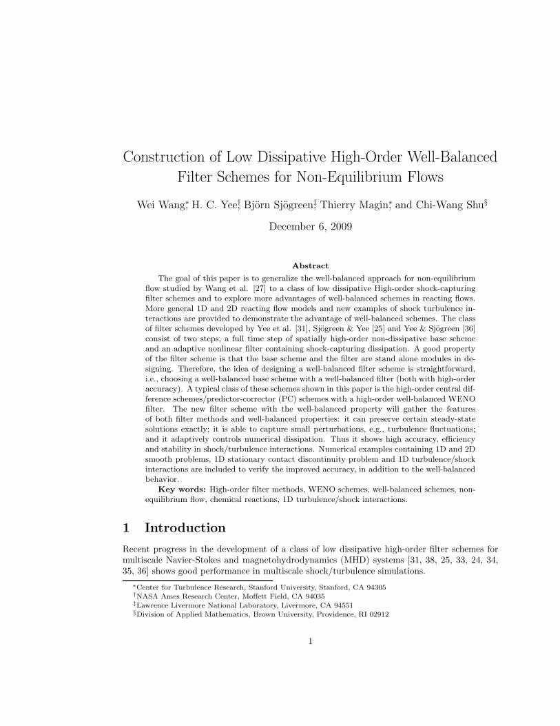
at t = 0. The other quantities are kept unperturbed. Fig. 1 shows the velocities by central andPC filter schemes of orders 2, 4, 6 and 8 at t = 0.1. The reference results are computed byfifth-order WENO-Roe with 1200 points and are considered to be “exact”.

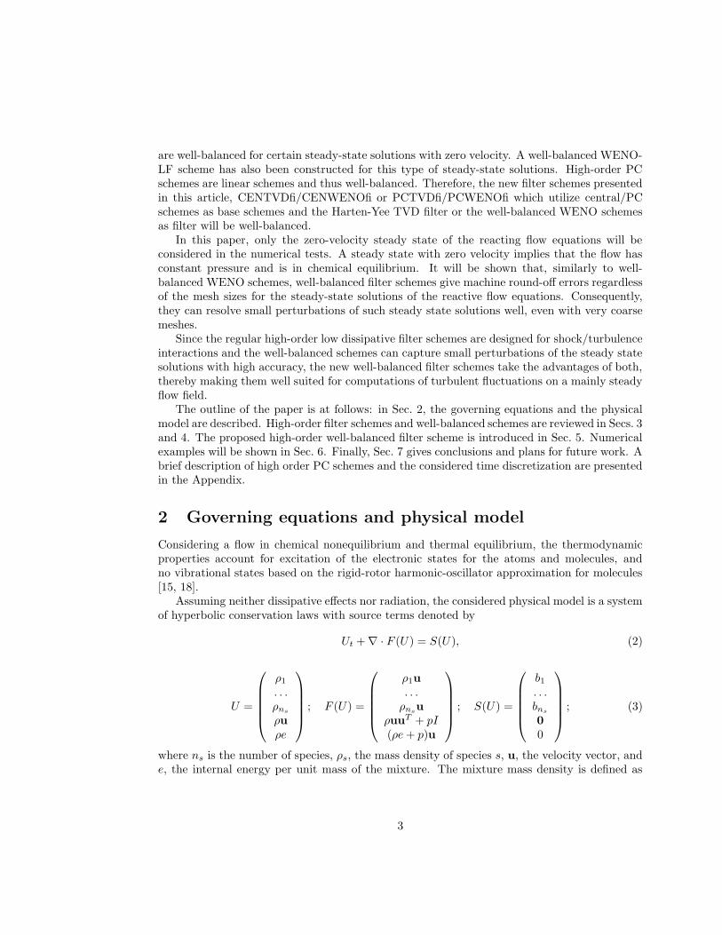
The results show that all the considered high-order well-balanced filter schemes can capturethe small perturbation well in a very coarse mesh. Especially for the schemes with order higherthan 2, only 50 points are used. However, the non well-balanced schemes behave in a veryoscillatory fashion, such as the regular WENO-LF with 200 points (Fig. 2). They can only

13

-1 -0.5 0 0.5 1

-0.0006

-0.0004

-0.0002

0

0.0002

0.0004

ReferenceCEN2TVDfi 200CEN4TVDfi 50CEN6WENO5fi 50CEN8WENO7fi 50

PSfrag replacements

x

u

-1 -0.5 0 0.5 1

-0.0006

-0.0004

-0.0002

0

0.0002

0.0004

ReferencePC2TVDfi 200PC4TVDfi 50PC6WENO5fi 50PC8WENO7fi 50

PSfrag replacements

xu

x

u

Figure 1: Small perturbation of velocity results by filter schemes: ε = 10−3×sin(πx). Solid linesare the reference 1200 point solution. Left: central filter schemes; Right: PC filter schemes.

resolve the solution when the mesh is refined enough such that the truncation error of thescheme is much smaller than the perturbation.

6.2.3 1D stationary contact discontinuity problem

The third example is a 1D stationary contact discontinuity problem on the domain [−5, 5].A stationary contact discontinuity is located at x = 0. The flow contains zero velocity andconstant pressure 20 N/m2 everywhere. The temperature has an initial condition

T =

{

500× (1 + 0.1 sin(2πx)), x < 0300× (1 + 0.1 sin(2πx)), x > 0

. (51)

The densities for each species can be solved by LTE condition. We add a small perturbationof the velocity over the whole domain

u′ = u+ 0.05× sin(πx). (52)

The computation stops at time t = 0.01. We remark that the solutions were computed on alarger domain [−6, 6] but truncated on [−5, 5] for not considering the effects by the boundarycondition. Figs. 3 and 4 show the densities, temperatures, velocities and pressures by thebalanced WENO-LF scheme and the regular WENO-LF scheme with 100 cells. The referencesolution is computed by the WENO-Roe scheme with 1200 cells. From Fig. 3 we can see thatthe balanced WENO-LF produces a more accurate result than the regular WENO-LF scheme.The regular WENO-LF scheme has a discrepancy from the reference solution on the waves andit cannot capture the small wave close to the shock. Unlike the density and temperature, thevelocity and pressure are constant at the initial time. Thus it is more clear to see the differencebetween the balanced WENO-LF and the regular WENO-LF on the velocity and pressureresults. From Fig. 4, we can see the results by the balanced WENO-LF are indistinguishablefrom the reference solution. However, the regular WENO-LF produces large oscillations due tothe truncation errors.

14

-1 -0.5 0 0.5 1

-0.0006

-0.0004

-0.0002

0

0.0002

0.0004

PSfrag replacements

x

u

Figure 2: Small perturbation of velocity results by WENO-LF scheme: ε = 10−3 × sin(πx).WENO-LF 200 points: dash-dot; Reference 1200 points: solid.

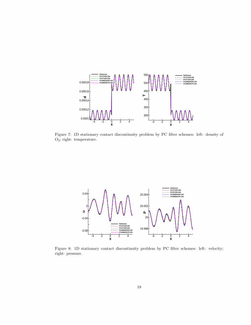
Figs. 5 and 6 show the results by the central filter schemes. The considered central fil-ter schemes here are CEN2TVDfi and CEN4TVDfi with 200 cells, and CEN6WENO5fi andCEN8WENO7fi with 100 cells. Similar for PC filter schemes, the results by PC2TVDfi,PC4TVDfi with 200 cells and PC6WENO5fi and PC8WENO7fi with 100 cells are shown inFigs. 7 and 8. All the well-balanced central/PC filter schemes can capture the small perturba-tions very well.

6.2.4 1D shock/turbulence interaction problem

The fourth example is a 1D shock/turbulence interaction problem (also referred to as the Shu-Osher problem [23]) for reacting flows on the domain [−5, 5]. Initially a shock is located atx = −4. The shock is moving at the speed 500 m/s to the right. The right state of the flowconsists two parts, the first part is a constant equilibrium state from -4 to 1 and the second partis an oscillatory equilibrium state from 1 to 5 with sine waves in densities and temperature.The conditions are given by

(TR, pR, uR) =

{

(500, 20, 0), x ∈ [−4, 1](500× (1 + 0.1 sin(2πx)), 20, 0), x ∈ [1, 5]

. (53)

Given the temperature and pressure, the densities for each species at the LTE state can beuniquely determined by the LTE condition. The left equilibrium state can be calculated ac-cording to the Rankine-Hugoniot jump condition.

Since the right state of the flow is a zero-velocity LTE state, the well-balanced schemes canresolve it with machine round-off errors. If we add a small perturbation of the velocity all overthe right state

u′ = u+ 10−3 × sin(πx), x ∈ [−4, 5], (54)

the well-balanced schemes will be able to capture this small perturbation very well.

15

x

d

-4 -2 0 2 40.0001

0.00012

0.00014

0.00016

0.00018

Referencebalanced WENO-LF 100WENO-LF 100

x

T

-4 -2 0 2 4

300

350

400

450

500

550 Referencebalanced WENO-LF 100WENO-LF 100

Figure 3: 1D stationary contact discontinuity problem by WENO-LF schemes: left: density ofO2; right: temperature.

x

u

-4 -2 0 2 4

-0.08

-0.04

0

0.04


x

p

-4 -2 0 2 4

19.998

20

20.002

20.004


Figure 4: 1D stationary contact discontinuity problem by WENO-LF schemes: left: velocity;right: pressure.

16

x

d

-4 -2 0 2 40.0001

0.00012

0.00014

0.00016

0.00018


x

T

-4 -2 0 2 4

300

350

400

450

500

550 ReferenceCEN2TVDfi 200CEN4TVDfi 200CEN6WENO5fi 100CEN8WENO7fi 100

Figure 5: 1D stationary contact discontinuity problem by central filter schemes: left: densityof O2; right: temperature.

x

u

-4 -2 0 2 4

-0.08

-0.04

0

0.04


x

p

-4 -2 0 2 4

19.998

20

20.002

20.004


Figure 6: 1D stationary contact discontinuity problem by central filter schemes: left: velocity;right: pressure.

17

x

d

-4 -2 0 2 40.0001

0.00012

0.00014

0.00016

0.00018


x

T

-4 -2 0 2 4

300

350

400

450

500

550 ReferencePC2TVDfi 200PC4TVDfi 200PC6WENO5fi 100PC8WENO7fi 100

Figure 7: 1D stationary contact discontinuity problem by PC filter schemes: left: density ofO2; right: temperature.

x

u

-4 -2 0 2 4

-0.08

-0.04

0

0.04


x

p

-4 -2 0 2 4

19.998

20

20.002

20.004


Figure 8: 1D stationary contact discontinuity problem by PC filter schemes: left: velocity;right: pressure.

18

x

u

-4 -2 0 2 40

20

40

60

80


zoomed in

x

u

-5 -4 -3 -2 -1

84.695

84.7

84.705

84.71


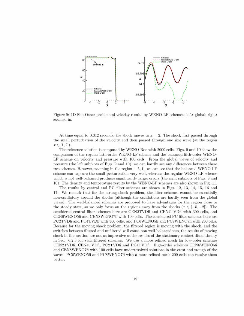
Figure 9: 1D Shu-Osher problem of velocity results by WENO-LF schemes: left: global; right:zoomed in.

At time equal to 0.012 seconds, the shock moves to x = 2. The shock first passed throughthe small perturbation of the velocity and then passed through one sine wave (at the regionx ∈ [1, 2]).

The reference solution is computed by WENO-Roe with 2000 cells. Figs. 9 and 10 show thecomparison of the regular fifth-order WENO-LF scheme and the balanced fifth-order WENO-LF scheme on velocity and pressure with 100 cells. From the global views of velocity andpressure (the left subplots of Figs. 9 and 10), we can hardly see any differences between thesetwo schemes. However, zooming in the region [−5, 1], we can see that the balanced WENO-LFscheme can capture the small perturbation very well, whereas the regular WENO-LF schemewhich is not well-balanced produces significantly larger errors (the right subplots of Figs. 9 and10). The density and temperature results by the WENO-LF schemes are also shown in Fig. 11.

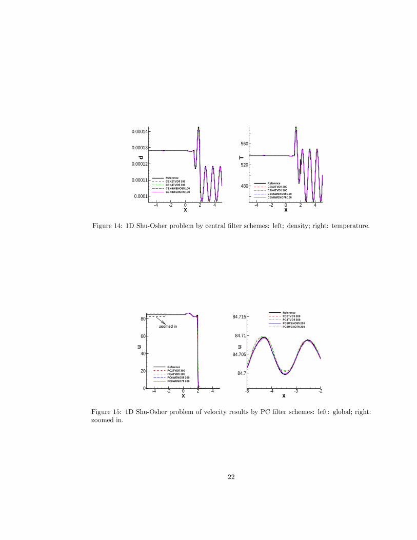
The results by central and PC filter schemes are shown in Figs. 12, 13, 14, 15, 16 and17. We remark that for the strong shock problem, the filter schemes cannot be essentiallynon-oscillatory around the shocks (although the oscillations are hardly seen from the globalviews). The well-balanced schemes are proposed to have advantages for the region close tothe steady state, so we only focus on the regions away from the shocks (x ∈ [−5,−2]). Theconsidered central filter schemes here are CEN2TVDfi and CEN4TVDfi with 300 cells, andCEN6WENO5fi and CEN8WENO7fi with 100 cells. The considered PC filter schemes here arePC2TVDfi and PC4TVDfi with 300 cells, and PC6WENO5fi and PC8WENO7fi with 200 cells.Because for the moving shock problem, the filtered region is moving with the shock, and theswitches between filtered and unfiltered will cause non well-balancedness, the results of movingshock in this section are not as impressive as the results of the stationary contact discontinuityin Sec. 6.2.3 for such filtered schemes. We use a more refined mesh for low-order schemesCEN2TVDfi, CEN4TVDfi, PC2TVDfi and PC4TVDfi. High-order schemes CEN6WENO5fiand CEN8WENO7fi with 100 cells have underresolved solutions in the crest and trough of thewaves. PC6WENO5fi and PC8WENO7fi with a more refined mesh 200 cells can resolve thembetter.

19

x

p

-4 -2 0 2 420

22

24

26


zoomed in

x

p

-5 -4 -3 -2 -1

25.878

25.8785

25.879


Figure 10: 1D Shu-Osher problem of pressure results by WENO-LF schemes: left: global; right:zoomed in.

x

d

-4 -2 0 2 4

0.0001

0.00011

0.00012

0.00013

0.00014


x

T

-4 -2 0 2 4

480

520

560


Figure 11: 1D Shu-Osher problem by WENO-LF schemes: left: density; right: temperature.

20

x

u

-4 -2 0 2 40

20

40

60

80

ReferencePC8WENO7fi 100CEN2TVDfi 300CEN4TVDfi 300CEN6WENO5fi 100CEN8WENO7fi 100

zoomed in

x

u

-5 -4 -3 -2

84.7

84.705

84.71

84.715ReferenceCEN2TVDfi 300CEN4TVDfi 300CEN6WENO5fi 100CEN8WENO7fi 100

Figure 12: 1D Shu-Osher problem of velocity results by central filter schemes: left: global;right: zoomed in.

x

p

-4 -2 0 2 420

22

24

26


zoomed in

x

p

-5 -4 -3 -2

25.878

25.8785

25.879 ReferenceCEN2TVDfi 300CEN4TVDfi 300CEN6WENO5fi 100CEN8WENO7fi 100

Figure 13: 1D Shu-Osher problem of pressure results by central filter schemes: left: global;right: zoomed in.

21

x

d

-4 -2 0 2 4

0.0001

0.00011

0.00012

0.00013

0.00014


x

T

-4 -2 0 2 4

480

520

560


Figure 14: 1D Shu-Osher problem by central filter schemes: left: density; right: temperature.

x

u

-4 -2 0 2 40

20

40

60

80


zoomed in

x

u

-5 -4 -3 -2

84.7

84.705

84.71

84.715ReferencePC2TVDfi 300PC4TVDfi 300PC6WENO5fi 200PC8WENO7fi 200

Figure 15: 1D Shu-Osher problem of velocity results by PC filter schemes: left: global; right:zoomed in.

22

x

p

-4 -2 0 2 420

22

24

26


zoomed in

x

p

-5 -4 -3 -2

25.878

25.8785

25.879 ReferencePC2TVDfi 300PC4TVDfi 300PC6WENO5fi 200PC8WENO7fi 200

Figure 16: 1D Shu-Osher problem of pressure results by PC filter schemes: left: global; right:zoomed in.

x

d

-4 -2 0 2 4

0.0001

0.00011

0.00012

0.00013

0.00014


x

T

-4 -2 0 2 4

480

520

560


Figure 17: 1D Shu-Osher problem by PC filter schemes: left: density; right: temperature.

23

-4 -2 0 2 4

500

1000

1500

2000

2500

3000

PSfrag replacements

x

T

-4 -2 0 2 40

100

200

300

400

500

PSfrag replacements

xT

x

u

-4 -2 0 2 4

0.75

0.755

0.76

0.765

PSfrag replacements

xTxu

x

y N2

Figure 18: Shock tube problem by CEN6WENO5fi: Left: temperature; Middle: velocity; Right:mass fraction of N2 (CEN6WENO5fi with 300 points: dash-dot; Reference 1200 points: solid).

6.2.5 A shock tube problem

The last 1D example is a shock tube problem. A diaphragm is located at x = 0 which separatesthe right chamber from the left chamber. The right chamber has cold air with pressure 0.6 ×105 N/m2 and temperature 300K. The gas in the left chamber has high pressure 6× 105 N/m2

and high temperature 3000K. Both gases are in LTE condition. The computational domain is[−5, 5] in the lab frame.

The results are computed at t = 0.001. The solution is no longer in steady state. Thisexample is to test the shock capturing ability of our well-balanced filter schemes. The numericalresults of temperature, velocity and mass fraction of N2 (from left to right) computed byCEN6WENO5fi, CEN8WENO7fi, PC6WENO5fi and PC8WENO7fi are plotted in Figs. 18,19, 20 and 21. As expected, the rarefaction wave, contact surface and shock appear in thetemperature solution. Since the velocity is consistent through the contact surface, there are onlyrarefaction wave and shock appearing in the velocity solution. Furthermore, mass is conservedduring the shock. No shock appears in the mass solution. All the considered well-balancedfilter schemes can capture the shocks sharply without oscillations.

6.3 Two dimensional numerical results

As mentioned in the beginning, extending the well-balanced schemes to the zero-velocity steadystate of 2D reacting flow is trivial because the reacting term does not depend explicitly on thespatial coordinates. In this section, similar well-balanced tests to 2D reacting flow will beperformed.

6.3.1 2D Well-balanced test

Similar to the 1D case, the first example is to check that the proposed schemes maintain the2D zero-velocity steady state exactly. The 2D special stationary case

T = 1000× (1 + 0.2 sin(π(x + y))) K, p = 105 N/m2, u = 0 m/s, (55)

24

-4 -2 0 2 4

500

1000

1500

2000

2500

3000

PSfrag replacements

x

T

-4 -2 0 2 40

100

200

300

400

500

PSfrag replacements

xT

x

u

-4 -2 0 2 4

0.75

0.755

0.76

0.765

PSfrag replacements

xTxu

x

y N2

Figure 19: Shock tube problem by CEN8WENO7fi: Left: temperature; Middle: velocity; Right:mass fraction of N2 (CEN8WENO7fi with 300 points: dash-dot; Reference 1200 points: solid).

-4 -2 0 2 4

500

1000

1500

2000

2500

3000

PSfrag replacements

x

T

-4 -2 0 2 40

100

200

300

400

500

PSfrag replacements

xT

x

u

-4 -2 0 2 4

0.75

0.755

0.76

0.765

PSfrag replacements

xTxu

x

y N2

Figure 20: Shock tube problem by PC6WENO5fi: Left: temperature; Middle: velocity; Right:mass fraction of N2 (PC6WENO5fi with 300 points: dash-dot; Reference 1200 points: solid).

-4 -2 0 2 4

500

1000

1500

2000

2500

3000

PSfrag replacements

x

T

-4 -2 0 2 40

100

200

300

400

500

PSfrag replacements

xT

x

u

-4 -2 0 2 4

0.75

0.755

0.76

0.765

PSfrag replacements

xTxu

x

y N2

Figure 21: Shock tube problem by PC8WENO7fi: Left: temperature; Middle: velocity; Right:mass fraction of N2 (PC8WENO7fi with 300 points: dash-dot; Reference 1200 points: solid).

25

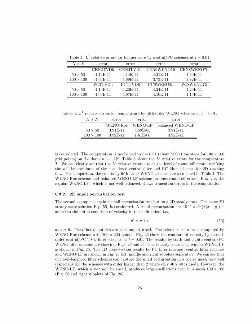
Table 3: L1 relative errors for temperature by central/PC schemes at t = 0.01.

N ×N error error error error

CEN2TVDfi CEN4TVDfi CEN6WENO5fi CEN8WENO7fi50 × 50 4.14E-11 4.14E-11 4.21E-11 4.30E-11

100× 100 4.04E-11 3.69E-11 3.73E-11 3.82E-11PC2TVDfi PC4TVDfi PC6WENO5fi PC8WENO7fi

50 × 50 4.13E-11 4.20E-11 4.24E-11 4.29E-11100× 100 4.03E-11 4.07E-11 4.10E-11 4.13E-11

Table 4: L1 relative errors for temperature by fifth-order WENO schemes at t = 0.01.

N ×N error error error

WENO-Roe WENO-LF balanced WENO-LF50 × 50 3.91E-11 4.59E-05 3.91E-11

100× 100 3.92E-11 1.61E-06 3.92E-11

is considered. The computation is performed to t = 0.01 (about 2000 time steps for 100× 100grid points) on the domain [−1, 1]2. Table 3 shows the L1 relative errors for the temperatureT . We can clearly see that the L1 relative errors are at the level of round-off errors, verifyingthe well-balancedness of the considered central filter and PC filter schemes for 2D reactingflow. For comparison, the results by fifth-order WENO schemes are also listed in Table 4. TheWENO-Roe scheme and balanced WENO-LF scheme produce round-off errors. However, theregular WENO-LF , which is not well-balanced, shows truncation errors in the computation.

6.3.2 2D small perturbation test

The second example is again a small perturbation test but on a 2D steady state. The same 2Dsteady-state solution Eq. (55) is considered. A small perturbation ε = 10−3 × sin(π(x + y)) isadded to the initial condition of velocity in the x direction, i.e.,

u′ = u+ ε (56)

at t = 0. The other quantities are kept unperturbed. The reference solution is computed byWENO-Roe scheme with 200 × 200 points. Fig. 22 show the contours of velocity by second-order central/PC TVD filter schemes at t = 0.01. The results by sixth and eighth central/PCWENO filter schemes are shown in Figs. 23 and 24. The velocity contour by regular WENO-LFis shown in Fig. 25. The 1D cross-section results by PC filter schemes, central filter schemesand WENO-LF are shown in Fig. 26 left, middle and right subplots separately. We can see thatour well-balanced filter schemes can capture the small perturbation in a coarse mesh very well(especially for the schemes with order higher than 2 where only 40× 40 is used). However, theWENO-LF, which is not well balanced, produces large oscillations even in a mesh 100 × 100(Fig. 25 and right subplots of Fig. 26).

26

-1 -0.5 0 0.5 1-1

-0.5

0

0.5

1

vel8E-054E-050

-4E-05-8E-05-0.00012-0.00016-0.0002-0.00024

PSfrag replacements

x

u

-1 -0.5 0 0.5 1-1

-0.5

0

0.5

1

vel8E-054E-050

-4E-05-8E-05-0.00012-0.00016-0.0002-0.00024PSfrag replacements

xu

x

u

Figure 22: 2D small perturbation of velocity results by filter schemes: ε = 10−3× sin(π(x+y)).Left: CEN2TVDfi 100× 100 points; right: PC2TVDfi 100× 100 points.

-1 -0.5 0 0.5 1-1

-0.5

0

0.5

1

vel8E-054E-050

-4E-05-8E-05-0.00012-0.00016-0.0002-0.00024

PSfrag replacements

x

u

-1 -0.5 0 0.5 1-1

-0.5

0

0.5

1

vel8E-054E-050


xu

x

u

Figure 23: 2D small perturbation of velocity results by central filter schemes: ε = 10−3 ×sin(π(x+ y)). Left: CEN6WENO5fi 40 × 40 points; right: CEN8WENO7fi 40 × 40 points.

27

-1 -0.5 0 0.5 1-1

-0.5

0

0.5

1

vel8E-054E-050

-4E-05-8E-05-0.00012-0.00016-0.0002-0.00024

PSfrag replacements

x

u

-1 -0.5 0 0.5 1-1

-0.5

0

0.5

1

vel8E-054E-050


xu

x

u

Figure 24: 2D small perturbation of velocity results by PC filter schemes: ε = 10−3× sin(π(x+y)). Left: PC6WENO5fi 40 × 40 points; right: PC8WENO7fi 40 × 40 points.

-1 -0.5 0 0.5 1-1

-0.5

0

0.5

1

vel8E-054E-050

-4E-05-8E-05-0.00012-0.00016-0.0002-0.00024

PSfrag replacements

x

u

Figure 25: 2D small perturbation of velocity results by WENO-LF schemes: ε = 10−3 ×sin(π(x+ y)). WENO-LF 100× 100 points.

28

u

-1 -0.5 0 0.5 1

-0.0002

-0.0001

0

0.0001

ReferenceCEN2TVDfi 100*100CEN4TVDfi 40*40CEN6WENO5fi 40*40CEN8WENO7fi 40*40

PSfrag replacements

xu

u

-1 -0.5 0 0.5 1

-0.0002

-0.0001

0

0.0001

ReferencePC2TVDfi 100*100PC4TVDfi 40*40PC6WENO5fi 40*40PC8WENO7fi 40*40

PSfrag replacements

xu

xu

u

-1 -0.5 0 0.5 1

-0.001

0

0.001

0.002 ReferenceWENO-LF 100*100

PSfrag replacements

xuxu

xu

Figure 26: Cross section of 2D velocity results at y = 0: ε = 10−3 × sin(π(x+ y)). Left: centralfilter schemes; middle: PC filter schemes; right: WENO-LF.

7 Concluding remarks

In this paper the well-balanced approach is extended to the high-order filter schemes in solvingfive species reacting flow in one and two space dimensions. This is a generalization of ourearlier work [27]. In addition, more general 1D and 2D reacting flow models and new examplesof shock turbulence interactions are provided to demonstrate the advantage of well-balancedschemes. Numerical examples are given to demonstrate the well-balanced property, accuracy,good capturing of the small perturbation of the steady-state solutions, and the non-oscillatoryshock resolution of the proposed well-balanced filter schemes. Because of the property of thezero-velocity steady-state solution of the reacting flow, the extension to any number of speciesand other reaction models is straightforward. Future research will consider the non-zero velocitysteady state and the advantages of well-balanced schemes to various steady-state problems.

Acknowledgments

The authors acknowledge the support of the DOE/SciDAC SAP grant DE-AI02-06ER25796.Partial of the work by the second author is performed under the NASA Fundamental Aero-nautics Hypersonic Program. The work by the third author is performed under the auspices ofthe U.S. Department of Energy by Lawrence Livermore National Laboratory under ContractDE-AC52-07NA27344, LLNL-JRNL-420355.

A Predictor-Corrector schemes and other spatial base schemes

Samples of the high-order base schemes for Fx can be of the following types.Central difference operators:CEN4:

Fx ≈1

12∆x(Fj+2 − 8Fj+1 + 8Fj−1 − Fj−2), (57)

29

CEN6:

Fx ≈1

60∆x(Fj+3 − 9Fj+2 + 45Fj+1 − 45Fj−1 + 9Fj−2 − Fj−3). (58)

Compact central difference operators (Hirsh [8], Ciment and Leventhal [4], and Lele [12]). Here

Fx ≈1

∆x(A−1

x BxF )j , (59)

where for a fourth-order approximation

(AxF )j = 16 (Fj+1 + 4Fj + Fj−1),

(BxF )j = 12 (Fj+1 − Fj−1),

(60)

and a sixth-order approximation

(AxF )j = 15 (Fj+1 + 3Fj + Fj−1),

(BxF )j = 160 (Fj+2 + 28Fj+1 − 28Fj−1 − Fj−2).

(61)

Predictor-corrector difference operators:PC4:

DpFj = 16∆x (7Fj − 8Fj−1 + Fj−2) ,

DcFj = 16∆x (−7Fj + 8Fj+1 − Fj+2) ,

(62)

PC6:DpFj = 1

30∆x (37Fj − 45Fj−1 + 9Fj−2 − Fj−3) ,DcFj = 1

30∆x (−37Fj + 45Fj+1 − 9Fj+2 + Fj+3) ,(63)

and PC8:

DpFj = 1420∆x (533Fj − 672Fj−1 + 168Fj−2 − 32Fj−3 + 3Fj−4) ,

DcFj = 1420∆x (−533Fj + 672Fj+1 − 168Fj+2 + 32Fj+3 − 3Fj+4) ,

(64)

where DpF is the PC differencing operator approximating Fx at the first step (predictor step)and DcF is the PC differencing operator at the second step (corrector step). New forms of theupwind biased PC methods including compact formulations developed by Hixon and Turkel[9, 10] are also applicable as spatial base schemes. Interested readers should refer to their paperfor the various upwind-biased PC formulae. The choice of the time integrators for these typesof PC methods is more limited. For example, if second-order time accuracy is desired, then(62), (63) and (64) in conjunction with the appropriate second-order Runge-Kutta methodare analogous to the familiar 2-4, 2-6 and 2-8 MacCormack schemes developed by Gottlieb andTurkel [5] and Bayliss et al. [1]. Here the first number refers to the order of accuracy for the timediscretization and the second number refers to the order of accuracy or the spatial discretization.However, in this case one achieves the second-order time accuracy without dimensional splittingof the Strang type [26]. For higher than second-order time discretizations, only certain evenstage Runge-Kutta methods are applicable. For compatible fourth-order Runge-Kutta timediscretizations, see Hixon and Turkel for possible formulae. For example, the classical fourth-order Runge-Kutta is applicable provided one applies the predictor and the corrector step twicefor the four stages, i.e., the predictor step for the first and third stages and the corrector stepfor the second and fourth stages.

30

For the considered 1D system with source term (2), the predictor-corrector scheme with2nd-order implicit explicit Runge-Kutta in time takes the form

U (1) = Un − ∆tDpF (tn, Un) + ∆tS(tn, Un), (65)

Un+1 = ((U (1) + Un) − ∆tDcF (tn+1, U (1)) + ∆tS(tn+1, Un+1))/2, (66)

The PC operators are modified at boundaries in a stable way by the summation-by-part(SBP) operators [17, 16, 33]. If Db is the standard pth-order SBP for the centered differenceoperators, then the pth-order PC operators are modified as follows,

Fx ≈

{

DpFj , j = nb + 1, . . . , N(2Db −Dc)Fj , j = 1, . . . , nb

(67)

at the predictor step and

Fx ≈

{

DcFj , j = 1, . . . , N − nb

(2Db −Dp)Fj , j = N − nb + 1, . . . , N(68)

at the corrector step, where N is the number of grid points and nb is the number of points thatneed boundary modified difference operators.

References

[1] Bayliss, A., Parikh, P., Maestrello, L. & Turkel, E. 1985 A fourth-order schemefor the unsteady compressible Navier Stokes equations, ICASE Report No. 85-44.

[2] Bose, D. & Candler, G.V. 1996 Thermal rate constants of the N2+O→ NO+N reactionusing ab initio 3A′′ and 3A′ potential energy surfaces J. Chem. Phys. 104, 2825–2833.

[3] Bose, D. & Candler, G.V. 1997 Thermal rate constants of the O2+N→ NO+O reactionbased on the 2A′ and 4A′ potential-energy surfaces J. Chem. Phys. 107, 6136–6145.

[4] Ciment, M. & Leventhal, H. 1975 Higher order compact implicit schemes for the waveequation, Math Comp. 29, 985–994.

[5] Gottlieb, D & Turkel, E. 1976 Dissipative twofour methods for time dependent prob-lems, Math Comp. 30, 703–723.

[6] Gurvich, L.V., Veits, I.V. & Alcock, C.B. 1989 Thermodynamic properties of indi-vidual substances, volume 1: O, H/D,T/, F, Cl, Br, I, He, Ne, Ar, Kr, Xe, Rn, S, N, P,and their compounds, Part one: methods and computation, Part two: tables New York,Hemisphere Publishing Corp., 1989.

[7] Harten, A. 1978 The artificial compression method for computation of shocks and contactdiscontinuities: III. Self-adjusting hybrid schemes, Math. Comp. 32, 363–389.

[8] Hirsh, R. S. 1975 Higher order accurate difference solutions of fluid mechanics problemsby a compact differencing technique, J. Comp. Phys. 19, 90–109.

31

[9] Hixon, R. & Turkel, E. 1998 High-accuracy compact MacCormack-type schemes forcomputational aeroacoustics, AIAA-1998-365, Aerospace Sciences Meeting and Exhibit,36th, Reno, NV, Jan. 12-15, 1998.

[10] Hixon, R. & Turkel, E. 2000 Compact implicit MacCormack-type schemes with highaccuracy, J. Comp. Phys. 158, 51–70.

[11] Jiang, G. & Shu, C.-W. 1996 Efficient implementation of weighted ENO schemes, J.Comp. Phys. 126, 202–228.

[12] Lele, S. 1992 Compact finite difference schemes with spectral-like resolution, J. Comp.Phys. 103, 16–42.

[13] LeVeque, R. J. 1998 Balancing source terms and flux gradients in high-resolution Go-dunov methods: the quasi-steady wave-propagation algorithm, J. Comp. Phys. 146, 346–365.

[14] LeVeque, R. J. & Yee, H. C. 1990 A study of numerical methods for hyperbolicconservation laws with stiff source terms, J. Comp. Phys. 86, 187–210.

[15] Magin, T. E., Caillault, L., Bourdon, A., & Laux, C. O. 2006 Nonequilibriumradiative heat flux modeling for the Huygens entry probe, J. Geophys. Res. 111, E07S12.

[16] Nordstrom, J. & Carpenter, M. H. 1999 Boundary and interface conditions for high-order finite-difference schemes applied to the Euler and Navier-Stokes equations, J. Comp.Phys. 148, 621–645.

[17] Olsson, P. 1995 Summation by parts, projections and stability I, Math. Comput. 64,1035–1065.

[18] Panesi, M., Magin, T. E., Bourdon, A., Bultel, A. & Chazot, O. 2009 Analysisof the FIRE II flight experiment by means of a collisional radiative model, J. of Thermo-physics and Heat Transfer 23, 236–248.

[19] Park, C. 1993 Review of chemical-kinetic problems of future NASA missions. I - Earthentries J. of Thermophysics and Heat Transfer 7, 385–398.

[20] Park, C., Jaffe, R.L. & Partridge, H. 2001 Chemical-kinetic parameters of hyper-bolic Earth entry J. of Thermophysics and Heat Transfer 15, 76–90.

[21] Qiu, J., Khoo, B. C. & Shu, C.-W. 2006 A numerical study for the performance ofthe Runge-Kutta discontinuous Galerkin method based on different numerical fluxes, J.Comp. Phys. 212, 540–565.

[22] Roe, P. L. 1981 Approximate Riemann solvers, parameter vectors, and difference schemes,J. Comp. Phys. 43, 357–372.

[23] Shu, C.-W. & Osher, S. 1989 Efficient implementation of essentially non-oscillatoryshock capturing schemes, II, J. Comp. Phys. 83, 32–78.

32

[24] Sjogreen, B. & Yee, H. C. Efficient low dissipative high order schemes for multiscaleMHD flows, I: Basic theory, AIAA 2003-4118, in: Proceedings of the 16th AIAA/CFDConference, 23-26 June 2003, Orlando, FL.

[25] Sjogreen, B. & Yee, H. C. 2004 Multiresolution wavelet based adaptive numericaldissipation control for shock-turbulence computation, RIACS Technical Report TR01.01,NASA Ames research center (Oct 2000); J. Sci. Comp. 20, 211–255.

[26] Strang, G. 1968 On the construction and comparison of difference schemes, SIAM J.Numer. Anal. 5, 506–517.

[27] Wang, W., Shu, C.-W., Yee, H. C.& Sjogreen, B. 2009 High order well-balancedschemes and applications to non-equilibrium flow, J. Comp. Phys., 228, 5787–5802.

[28] Xing, Y. & Shu, C.-W. 2005 High order finite difference WENO schemes with the exactconservation property for the shallow water equations, J. Comp. Phys. 208, 206–227.

[29] Xing, Y. & Shu, C.-W. 2006 High order well-balanced finite difference WENO schemesfor a class of hyperbolic systems with source terms, J. Sci. Comp. 27, 477–494.

[30] Yee, H. C. 1989 A class of high-resolution explicit and implicit shock-capturing methods,VKI lecture series 1989-04, March 6-10, 1989; NASA TM-101088, Feb. 1989.

[31] Yee, H. C., Sandham, N. D., & Djomehri, M. J. 1999 Low dissipative high ordershock-capturing methods using characteristic-based filters, J. Comp. Phys. 150, 199–238.

[32] Yee, H. C. & Shinn, J. L. 1989 Semi-implicit and fully implicit shock-capturing methodsfor nonequilibrium flows, AIAA Journal 225, 910–934.

[33] Yee, H. C. & Sjogreen, B. 2001 Designing Adaptive Low Dissipative High OrderSchemes for Long-Time Integrations, ”Turbulent Flow Computation”, D.Drikakis andB.Geurts (eds.), October 2001 .

[34] Yee, H. C. & Sjogreen, B. 2005 Efficient low dissipative high order scheme for mul-tiscale MHD flows, II: Minimization of Div(B) numerical error, RIACS Technical ReportTR03.10, July, 2003, NASA Ames Research Center; J. Sci. Comp. , DOI: 10.1007/ s10915-005-9004-5.

[35] Yee, H. C. & Sjogreen, B. 2006 Nonlinear Filtering and Limiting in High Order Meth-ods for Ideal and Non-ideal MHD, J. Sci. Comp 27, 507–521.

[36] Yee, H. C. & Sjogreen, B. 2007 Development of low dissipative high order filter schemesfor multiscale Navier-Stokes/MHD systems, J. Comp. Phys. 68, 151–179.

[37] Yee, H. C., Sweby, P. K. & Griffiths, D. F. 1991 Dynamical approach study ofspurious steady-state numerical solutions for non-linear differential equations, Part I: Thedynamics of time discretizations and its implications for algorithm development in com-putational fluid dynamics, J. Comp. Phys. 97, 249–310.

[38] Yee, H. C., Vinokur, M & Djomehri, M. J. 2000 Entropy Splitting and NumericalDissipation, J. Comp. Phys. 162, 33–81.

33

construction of low dissipative high-order well-balanced filter schemes for non-equilibrium flows

Documents