construction of fuzzy inference rules by ndf and …construction of fuzzy inference rules by ndf and...
TRANSCRIPT
Construction of Fuzzy Inference Rules by NDF
and NDFL Isao Hayashi, Hiroyoshi Nomura,
Hisayo Yamasaki, and Noboru Wakami Matsushita Electric Industrial Co., Ltd.,
Moriguchi, Osaka, Japan
A B S T R A C T
Whereas conventional fuzzy reasoning lacks determining membership functions, a neural network driven fuzzy reasoning (NDF) capable of determining member- ship functions uniquely by an artificial neural network is formulated. In an NDF algorithm the optimum membership function in the antecedent part of fuzzy inference rules is determined by a neural network, while in the consequent parts an amount of reasoning for each rule is determined by other plural neural networks. On the other hand, we propose a new algorithm that can adjust inference rules to compensate for a change of inference environment. We call this algorithm a neural network driven fuzzy reasoning with learning function (NDFL). NDFL can deter- mine the optimal membership function and obtain the coefficients of linear equations in the consequent parts by the searching function of the pattern search method. In this paper, inference rules for making a pendulum stand up from its lowest suspended point are determined by the NDF algorithm for verifying its effectiveness. The NDFL algorithm is formulated and applied to a simple numeri- cal example to demonstrate its effectiveness.
KEYWORDS: f u z zy reasoning, f u z zy logic, neural network, membership functions, learning function
I N T R O D U C T I O N
Extensive applications of fuzzy reasoning for various control problems have been reported (Hirota [1]). However, in these cases, fuzzy reasoning is generally involved with tuning problems (Lee [2]). That is, the form of the
Address correspondence to Isao Hayashi, Matsushita Electric Industrial Co., Ltd., Moriguchi, Osaka, 570, Japan.
International Journal of Approximate Reasoning 1992; 6:241-266 © 1992 Elsevier Science Publishing Co., Inc. 655 Avenue of the Americas, New York, NY 10010 0888-613X/92/$5.00 241

242 Isao Hayashi et al.
fuzzy number of antecedent and consequent parts of fuzzy inference rules has to be adjusted to minimize the difference between estimation of fuzzy reasoning and output data for a given input data.
A neural network driven fuzzy reasoning (NDF for short) (Hayashi et al. [3], Takagi and Hayashi [4]) by which inference rules are constructed from the learning function of neural networks (Anderson and Rosenfield [5], Tank and Hopplied [6]) for solving tuning problems was previously reported. NDF is a type of fuzzy reasoning having an error backpropagation type of neural network (Rumlhart et al. [7]) that represents fuzzy sets in its antecedent, while another plural error backpropagation type of neural network represents a relationship between input and output data of the consequent of each rule. NDF can obtain the optimal membership function and inference rules from the observed input-output data. However, NDF is unable to alter its inference rule when an environment for constructing that rule is dynamically changing. Thus, we propose a new algorithm that can adjust its inference rules in response to changes in the inference environment. We call this algorithm neural network driven fuzzy reasoning with learning function (NDFL). NDFL can determine the optimal membership function in the same way as NDF by a learning function of the error backpropagation type of neural network and obtain the coefficients of linear equations (Sugeno and Kang [8]) in the consequent parts by the searching function of the pattern search method (Hooke and Jeeves [9]).
In this paper, an algorithm for constructing inference rules based on NDF is introduced first, and an experimental verification of its effectiveness is per- formed taking as an example an inverted pendulum system. Furthermore, the NDFL algorithm is formulated and applied to a simple numerical example to demonstrate its effectiveness. Since the fuzzy set of the antecedent and the input-output relationship between consequent parts can be determined by means of NDF and NDFL without fine tuning of inference rules by utilizing the neural network learning function acquired from the input-output data, it is advantageous to solve tuning problems of fuzzy reasoning.
N E U R A L NETWORK DRIVEN FUZZY R E A S O N I N G (NDF)
In NDF, the membership function in the antecedent part is determined in multidimensional space. For example, the conventional fuzzy inference rules for representing a fuzzy model (Sugeno and Kang [8]) shown below are considered.
Rl: IF x, is FSL and x 2 is FSL ,
R2: IFx I is FSL and x 2 is FI3 o,
THEN y ~= a~o + a , ~ x j + a12x 2
(la)
THEN y2= a20 + a2~x ~ + a 2 2 x 2
(lb)
Construction of Fuzzy Inference Rules 243
R3: IF x I is FB6, THEN y3-- a30 + a31x I ( lc)
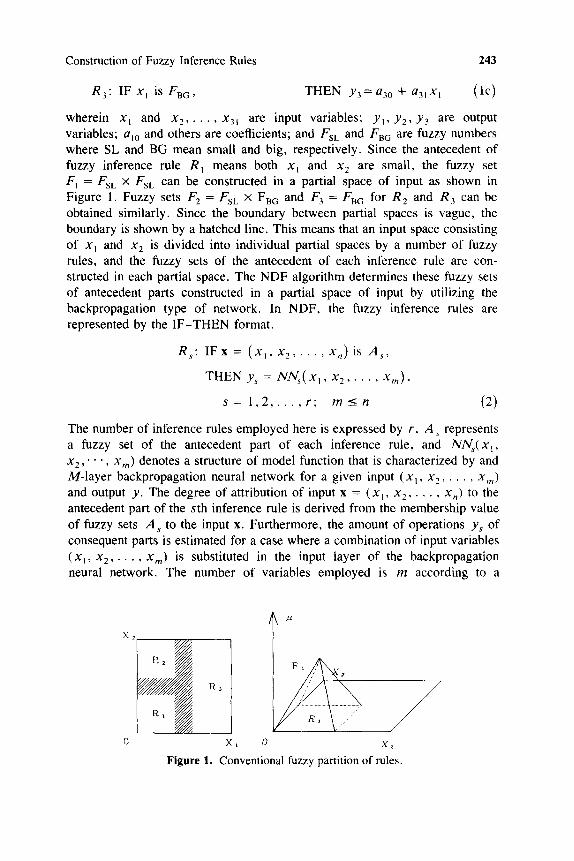
wherein x t and x 2 . . . . . x3~ are input variables; y~, Y2, Y3 are output variables; alo and others are coefficients; and FsL and Fac are fuzzy numbers where SL and BG mean small and big, respectively. Since the antecedent of fuzzy inference rule R I means both x t and x 2 are small, the fuzzy set F I = FSL X FSL can be constructed in a partial space of input as shown in Figure 1. Fuzzy sets F 2 = FsL X FBG and F 3 = FBc for R 2 and R 3 can be obtained similarly. Since the boundary between partial spaces is vague, the boundary is shown by a hatched line. This means that an input space consisting of x~ and x 2 is divided into individual partial spaces by a number of fuzzy rules, and the fuzzy sets of the antecedent of each inference rule are con- structed in each partial space. The NDF algorithm determines these fuzzy sets of antecedent parts constructed in a partial space of input by utilizing the backpropagation type of network. In NDF, the fuzzy inference rules are represented by the I F - T H E N format.
Rs: I F x = ( x I , x 2 . . . . . xn) is A s,
THEN Ys = NNs( x t , x2 . . . . . xm),
s = 1 ,2 . . . . . r ; m < n (2)
The number of inference rules employed here is expressed by r, A s represents a fuzzy set of the antecedent part of each inference rule, and NNs(X ~, x2," • . , x m) denotes a structure of model function that is characterized by and M-layer backpropagation neural network for a given input ( x I, x 2 . . . . . Xm) and output y. The degree of attribution of input x = (x~, x 2 . . . . . x n) to the antecedent part of the sth inference rule is derived from the membership value of fuzzy sets A s to the input x. Furthermore, the amount of operations Ys of consequent parts is estimated for a case where a combination of input variables (x~, x 2 . . . . . Xm) is substituted in the input layer of the backpropagation neural network. The number of variables employed is m according to a
X~ T R3
X1 0
Figure 1. Conventional fuzzy partition of X~
rules.
244 Isao Hayashi et al.
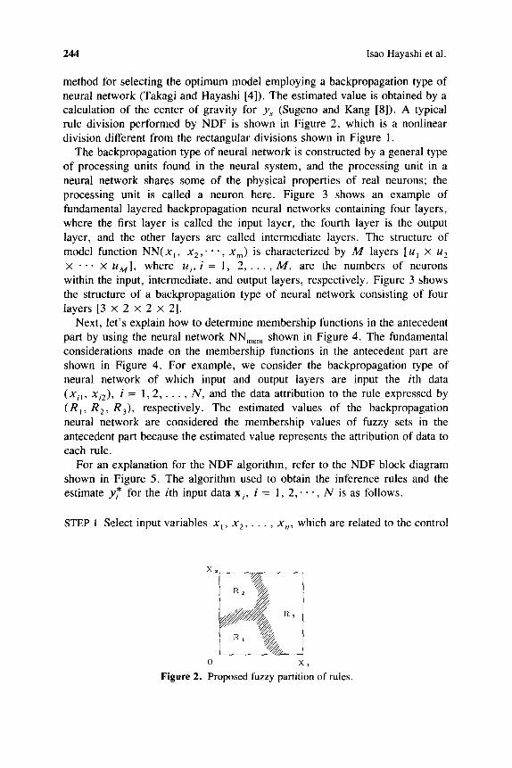
method for selecting the optimum model employing a backpropagation type of neural network (Takagi and Hayashi [4]). The estimated value is obtained by a calculation of the center of gravity for Ys (Sugeno and Kang [8]). A typical rule division performed by NDF is shown in Figure 2, which is a nonlinear division different from the rectangular divisions shown in Figure 1.
The backpropagation type of neural network is constructed by a general type of processing units found in the neural system, and the processing unit in a neural network shares some of the physical properties of real neurons; the processing unit is called a neuron here. Figure 3 shows an example of fundamental layered backpropagation neural networks containing four layers, where the first layer is called the input layer, the fourth layer is the output layer, and the other layers are called intermediate layers. The structure of model function NN(x~, x 2 , ' " , x m) is characterized by M layers [u~ x u 2 x . . . x uM], where u i, i = l , 2 . . . . . M , are the numbers of neurons within the input, intermediate, and output layers, respectively. Figure 3 shows the structure of a backpropagation type of neural network consisting of four layers [3 x 2 x 2 x 2].
Next, let's explain how to determine membership functions in the antecedent part by using the neural network NNme m shown in Figure 4. The fundamental considerations made on the membership functions in the antecedent part are shown in Figure 4. For example, we consider the backpropagation type of neural network of which input and output layers are input the ith data ( x i j , xi2), i = 1 ,2 . . . . . N , and the data attribution to the rule expressed by ( R j , R 2, R3) , respectively. The estimated values of the backpropagation neural network are considered the membership values of fuzzy sets in the antecedent part because the estimated value represents the attribution of data to each rule.
For an explanation for the NDF algorithm, refer to the NDF block diagram shown in Figure 5. The algorithm used to obtain the inference rules and the estimate y* for the ith input data xi, i = 1, 2 , . . ' , N is as follows.
STEP 1 Select input variables X l , X 2 . . . . . Xn , which are related to the control
Figure 2.
X2
0 X1
Proposed fuzzy partition of rules.

Construction of Fuzzy Inference Rules
(4
( \
1
Figure 3. Example of neural network.
245
value y. This is for an assumed case where the ith input-output data (y i , X i ) =
(Yi, XiI,Xi2 . . . . . Xin), i = 1 ,2 . . . . . N, are obtained and the input data x i j ,
where j = 1 ,2 . . . . . n, are the ith data of input variable x i .
STEP 2 Divide input-output data into r classes of R~, where s = 1 , 2 , . . . , r. As mentioned before, each partition is regarded as an inference rule R~, and the input-output data for each R s are expressed by (YT, x~), where i = 1,2 . . . . . N s, provided that N~ is a number of input-output data for each R s.
STEP 3 Determine membership functions in the antecedent part by using the neural network NNme m shown in Figure 5 provided that the structure of the backpropagation neural network is M- layered [n x u 2 x . . - x uA4_ ~ z r ] .
STEP 4 Determine models in the consequent part by using neural networks NN l, NN 2 . . . . , NN r shown in Figure 5 provided that the structure of each backpropagation type of network NN s is M- layered [ k × u 2 × • • • x u M_ x 1], k = n, n - 1 . . . . . 1, and select the optimum model for each NN s.
We propose the stepwise procedure for utilizing the backpropagation type of neural network for determining input variables in the consequent part. The stepwise procedure for utilizing the backpropagat ion type of neural network is described as follows.
STEP 4-1 Setting a condit ion at k = n, the input data x i = (X i l , Xi2 . . . . . X i k ) , i = 1 , 2 . . . . , N , are assigned for the input layer of each NNs, and the output data Yi is assigned for the output layer of each NNs, where the input variables assigned for the input and output layers are expressed respectively by

246 lsao Hayashi et al.
%:1
M
o
o
o o
o
E
Z
Z
/
2
e,-,
E
0

Construction of Fuzzy Inference Rules 247
N Nmem
A n l e c e d e n t
P a r t
Y E s t i m a t i o n
c 0 t . . . . . . . .
-~z h e y ( I ) mey(2 )
.5
_ . J J I ~ j
i n p u t V a r . X , X~ X~
Figure 5. Block diagram of neural network driven fuzzy reasoning.
I I !
m . y ( r )
Qs = {xl , x2 . . . . . xk} (3)
and
T, = {y} (4)
where Qs represents a set of input variables assigned for the input layer of each backpropagation type of neural network NN~, and T~ represents a set of output variables assigned for the output layer of NN~.
STEP 4-2 An estimation of e y i for the input data x i ~ , x i 2 . . . . . x i k can be obtained after repeated learnings made on the backpropagation neural network NN,. However, the number of learnings is set at approximately 3000. Then the sum of mean squared errors of output data Yi and the estimate e y i is calculated to obtain an evaluation value of J~ required for determining the input variables.
J~, = ( Y i - eY i / N , s = 1 , 2 . . . . . r (5) i = l
STEP 4-3 In order to determine the correlation of input variables xy to the output variables y, the input variable xy is temporarily removed from the set of input variables x t , x 2 . . . . . x k . The input data from which the input variable xj is removed, Xi l . . . . . x i j ~, x u + ~ . . . . . X i k , where i = 1,2 . . . . . N, are assigned to the input layer of the M-layer backpropagation neural network [k - 1 x u 2 x • .- x uM_~ x 1], and the output data yi are
248 Isao Hayashi et al.
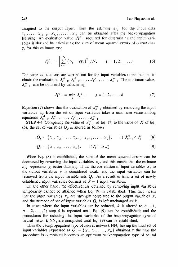
assigned to the output layer. Then the estimate eyf for the input data X i l , ' ' ' , Xij-I, Xij+l . . . . , xik can be obtained after the backpropagation learning. An evaluation value J~J-L required for determining the input vari- ables is derived by calculating the sum of mean squared errors of output data Yi for this estimate eyi:
J~{ ' = ( ~-~" ( Y i - eYi')2] I N ' i = , s = 1,2 . . . . . r (6)
The same calculations are carried out for the input variables other than Xj to
obtain the evaluations J~J_ 1, j~2 1 . . . . . J~J-J . . . . . J~k_ I . The minimum value, j~cj, can be obtained by calculating
j~c_, = minJ~S , j = 1 ,2 . . . . . k (7) J
Equation (7) shows that the evaluation of J ~ z obtained by removing the input variables x~ from the set of input variables takes a minimum value among equations J ~ ] l , j~2_j . . . . . j ~ j ] . . . . . j~k l .
STEP 4-4 Comparing the value of J ~ ] of Eq. (7) to the value of J~ of Eq. (5), the set of variables Qs is altered as follows.
Q~= { x , , x 2 . . . . . Xc_,,x,.+, . . . . . xk}, if J~'_, < J~ (8)
Qs = { x , , x 2 . . . . . x~}, ifJ~C,> J~ (9)
When Eq. (8) is established, the sum of the mean squared errors can be decreased by removing the input variables x c, and this means that the estimate ey, represents yj better than ey i. Thus, the correlation of input variables x c to the output variables y is considered weak, and the input variables can be removed from the input variable sets Qs. As a result of this, a set of newly established input variables consists of k - 1 input variables.
On the other hand, the effectiveness obtained by removing input variables temporarily cannot be attained when Eq. (9) is established. This fact means that the input variables xc are strongly correlated to the output variables y , and the number of set of input variables Qs is left unchanged as k.
In cases where the input variables can be reduced, k is altered to n - 1, n - 2 . . . . . 1; step 4 is repeated until Eq. (9) can be established; and the procedures for reducing the input variables of the backpropagation type of neural network NN s are completed until Eq. (9) can be established.
Thus the backpropagation type of neural network NN s having the final set of input variables expressed as Q~ = { x], x2 . . . . . Xr,,} obtained at the time the procedure is completed becomes an optimum backpropagation type of neural
Construction of Fuzzy Inference Rules 249
network representing the structure of the consequent part of the rule R s. The same step procedure is conducted for each NNs to determine the consequent parts of all the inference rules.
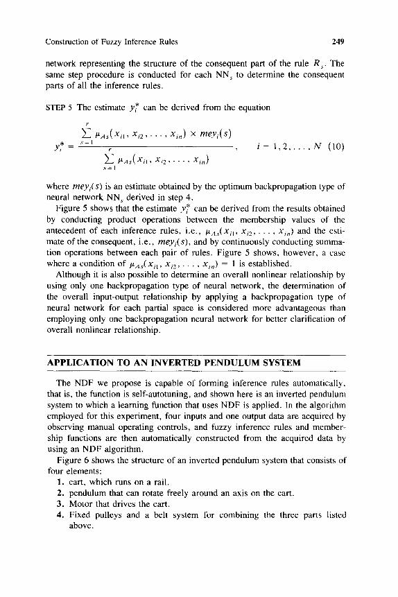
STEP 5 The estimate y* can be derived from the equation
£ tzA (Xi,. Xi2 . . . . . X,.) X meYi(S ) Y t = * : ' . . . . .
s - 1
i = 1,2 . . . . . N (10)
where meYi(S ) is an estimate obtained by the optimum backpropagation type of neural network NN s derived in step 4.
Figure 5 shows that the estimate y* can be derived from the results obtained by conducting product operations between the membership values of the antecedent of each inference rules, i.e., #As(Xi l , Xi2 . . . . . Xi,,) and the esti- mate of the consequent, i.e., meYi(S) , and by continuously conducting summa- tion operations between each pair of rules. Figure 5 shows, however, a case where a condition of I, LAs(Xil, Xi2 . . . . . Xin ) = 1 is established.
Although it is also possible to determine an overall nonlinear relationship by using only one backpropagation type of neural network, the determination of the overall input-output relationship by applying a backpropagation type of neural network for each partial space is considered more advantageous than employing only one backpropagation neural network for better clarification of overall nonlinear relationship.
A P P L I C A T I O N TO A N I N V E R T E D P E N D U L U M SYSTEM
The NDF we propose is capable of forming inference rules automatically, that is, the function is self-autotuning, and shown here is an inverted pendulum system to which a learning function that uses NDF is applied. In the algorithm employed for this experiment, four inputs and one output data are acquired by observing manual operating controls, and fuzzy inference rules and member- ship functions are then automatically constructed from the acquired data by using an NDF algorithm.
Figure 6 shows the structure of an inverted pendulum system that consists of four elements:
1. cart, which runs on a rail. 2. pendulum that can rotate freely around an axis on the cart. 3. Motor that drives the cart. 4. Fixed pulleys and a belt system for combining the three parts listed
above.

250 Isao Hayashi et al.
The pendulum angle apart from the perpendicular 0 degree and the distance from the original cart position are detected by the potentiometers a and b, respectively, shown in Figure 6. These values are digitized by an A/D converter and are fed to a personal computer wherein the velocities of inverted pendulum angle and the cart distance are derived from the four variables, pendulum angle, angular velocity, cart distance, and cart velocity by using
an NDF algorithm. As the motor control signal derived by the personal computer takes a digital form, it is converted into an analog value through a D/A converter.
The configuration of the inverted pendulum system and the control computer are as follows.
Body of the inverted pendulum system
Pendulum Drive force Sensors
Microcomputer Program
Length 1410 mm, width 400 mm, height 880 mm Length 400 mm, weight 40 g, diameter 4 mm 25-W dc motor with gear ratio of 12.5:1 Potentiometer to measure the distance from the original position of the cart, and another to measure the pendulum angle. CPU 80286 C language, 21K bytes
The inverted pendulum system has two control areas--a linear control area where the pendulum stands upright, and a nonlinear control area where the pendulum falls. We constructed an inverted pendulum system in the linear
a b
Personal c o l p u t e r
C o n t r o l ]
Figure 6. Structure of inverted pendulum system.
Construction of Fuzzy Inference Rules 251
control area by using a convent iona l fuzzy control , and a control mode l in the
nonl inear control area by uti l izing N D F .
Contro l rules appl icable to the inver ted pendulum were formula ted accord-
ing to an a lgor i thm deve loped for cons t ruc t ing the inference rules by applying
N D F descr ibed in the fo l lowing.
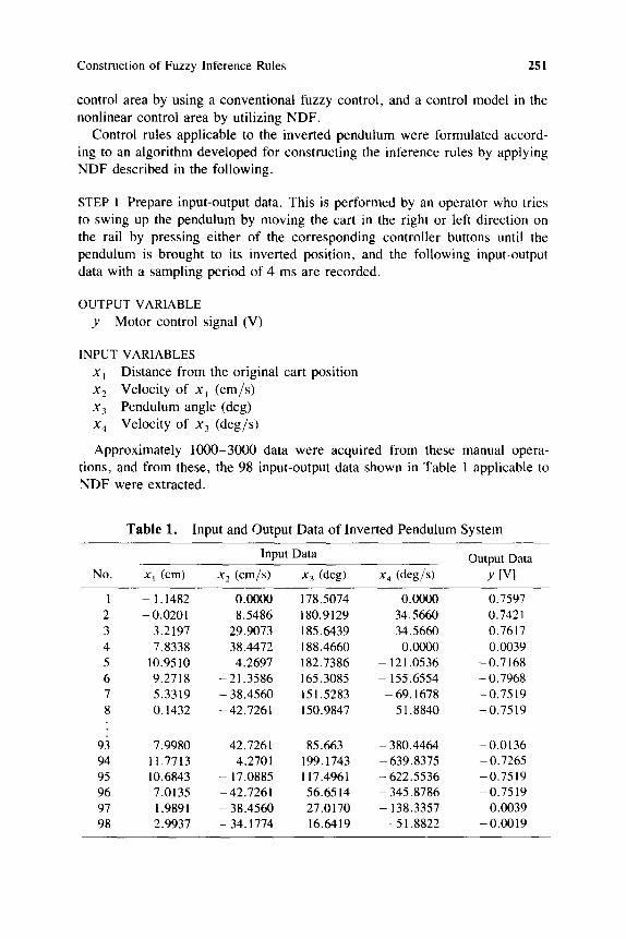
STEP 1 Prepare input-output data. This is pe r fo rmed by an opera tor who tries
to swing up the pendulum by m o v i n g the cart in the right or left direct ion on
the rail by press ing e i ther o f the cor responding cont ro l le r buttons until the
pendulum is brought to its inver ted posi t ion, and the fo l lowing input-output
data with a sampling per iod o f 4 ms are recorded.
OUTPUT VARIABLE
y Moto r control signal (V)
INPUT VARIABLES
x j Dis tance f rom the or iginal cart posit ion
x 2 Veloc i ty o f x I ( c m / s )
x 3 Pendu lum angle (deg)
x 4 Veloc i ty o f x 3 (deg / s )
Approx ima te ly 1 0 0 0 - 3 0 0 0 data were acqui red f rom these manual opera-
t ions, and f rom these, the 98 input-output data shown in Table 1 appl icable to
N D F were extracted.
T a b l e 1. Input and Output Data o f Inver ted Pendulum System
Input Data Output Data
No. x I (cm) xe (cm/s) x 3 (deg) x 4 (deg/s) y [V]
1 - 1.1482 0.0000 178.5074 0.0000 0.7597 2 -0 .0201 8.5486 180.9129 34.5660 0.7421 3 3.2197 29.9073 185.6439 34.5660 0.7617 4 7.8338 38.4472 188.4660 0.0000 0.0039 5 10.9510 4.2697 182.7386 - 121.0536 - 0.7168 6 9.2718 - 21.3586 165.3085 - 155.6554 - 0.7968 7 5.3319 - 38.4560 151.5283 - 69.1678 -0 .7519 8 0.1432 -42.7261 150.9847 51.8840 - 0.7519
93 7.9980 42.7261 85.663 - 380.4464 -0 .0136 94 11.7713 4.2701 199.1743 - 639.8375 - 0.7265 95 10.6843 - 17.0885 117.4961 - 622.5536 -0 .7519 96 7.0135 - 42.7261 56.6514 -345 .8786 - 0.7519 97 1.9891 - 38.4560 27.0170 - 138.3357 0.0039 98 - 2.9937 - 34.1774 16.6419 - 51.8822 - 0.0019

252 Isao Hayashi et al.
STEP 2 Set two rules for the input-output data containing the data distributions.
STEP 3 Determine the membership functions of the antecedent part. A three- layer [4 x 6 x 2] backpropagation type of neural network is employed here for determining the antecedent part construction, and the number of learnings is set at 1500.
STEP 4 Determine the consequent part structure. A three-layer [k x 6 × 1], k = 4, 3, 2, 1, backpropagation type of neural network for determining the consequent part structure is employed here, and the number of learnings of each backpropagation type of network is set at 3500.
By using a stepwise procedure for utilizing backpropagation type neural networks, we obtain
J2 = 0.016 (11)
~l, = min j i j (= 0.007), j = 1 , 2 , 3 , 4 (12) J
Therefore,
J~' < J] (13)
By removing the input variables xj , we obtained Qs = { x2, x3, x4}- As for Qs = { x2, x3, x4}, the following can be obtained.
j l l = 0 . 0 0 7 ( 1 4 )
~13 = min J~J(= 0.021), j = 1 , 2 , 3 , 4 (15)
This means
J213 > J~' (16)
Thus, the number of input variables is not reduced, and the algorithm for rule 1 is completed by the second calculation process. The algorithm for rule 2 is completed by the second calculation process in the same way. The inference rules consequently obtained by these are
Rj: IFx = ( x I , x 2 , x 3 ,x4) is A I,
THEN y, = NNI(X 2 , x 3, x4) (17a)
R2: IF x = ( x l , x2, x3, x4) is A2,
THEN Y2 = NN2(x, , x2, x4) (17b)
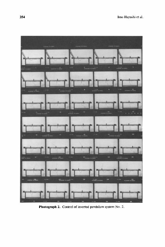
Photographs 1 and 2 show the swing-up motions of the pendulum controlled by fuzzy inference rules expressed by Eqs. (17a) and (17b). Photograph 1 shows sequential motions as the pendulum swung from its stable equilibrium state to an inverted standstill state. The estimate y* can be derived from Eq.

Construction of Fuzzy Inference Rules 253
Photograph 1. Control of inverted pendulum system No. 1.
254 Isao Hayashi et al.
Photograph 2. Control of inverted pendulum system No. 2.

Construction of Fuzzy Inference Rules 255
(10). The pendulum can be brought to its inverted position regardless of the cart position on the rail. Photograph 2 shows the other control of swing-up motion for given pendulum angles.
An experimental study of the robustness of control performed by NDF was carried out by changing the parameters that govern the dynamic characteristics of the controlled object, and the length of pendulum was taken as a parameter governing the dynamic characteristics of the pendulum here. The initial position of the cart was set at the center position of the belt on which the inverted pendulum device is mounted, and the pendulum angle was set at 0 ° when it was hung down initially and + 180" is specified when the pendulum was at an inverted position. The angle was incremented for clockwise rotation and decremented for counterclockwise rotation.
The inference rule was constructed for a case where the pendulum length was set at 40 cm, and Figure 7 shows the response of such a pendulum. Figures 8, 9, and 10 show the responses of pendulums 20, 30, and 50 cm long, respectively. These inference rules were constructed for a case where the pendulum length was set at 40 cm. The shifts of pendulum angle are shown by solid lines, and the changes of angular velocity are shown by broken lines in Figures 8-10. However, only the changes of pendulum angle and angular velocity until the pendulum comes to an inverted position, and no response after completion of inversion, are shown there. As for the learning of the inverted pendulum, the learning of the swing-up process was made for constructing an inference rule applicable to the process of a pendulum starting from a downward-hanging position and proceeding to a nearly inverted posi- tion. The inverted position is defined as a pendulum angle close to _+ 180", and its angular velocity is nearly zero at that time.
I ! :0 1 :~P
1i5
'i~O
4;
0
-:~'L1
- ] ~:5
l : iQ
- f \ ..
Angle
"... ~ ,/" ', \ /
'J/ Angle Veloc]
' ~;)L1
:?Ll
Ll
,!i)O
l.tl ~.0 i:.0 4.~
Figure 7. Angle and angle velocity of 40-cm long pendulum.

256 Isao Hayashi et al.
l:i:O
?~:. / ~ - -
90 . . / -
-.1', . / .{
" / g e el ':'~' ' I
- V : 0
120O
1 L : ~ 0 0
i!:20
280
0
- 2 0 ~ : 1
,100
:..00
- [ :-'[ol.l 0 /. [1 ?. 0 7:. 71
Figure 8. Angle and angle velocity of 30-cm long pendulum.
As shown in Figure 7, the pendulum reached the - 180 ° position in 4.6 s after the start of control, attaining an angular velocity of about 0° /s , and the pendulum stood still at the inverted position. This is a natural consequence because the inference rules were established for a 40-cm long pendulum.
Figure 8 shows a transient response of a pendulum 30 cm long. The pendulum was brought to its inverted position, showing a response similar to that obtained with the 40-cm pendulum, but the angle reached - 180 ° in 3.9 s. The overall controllable characteristics were similar to those of the 40-cm pendulum.
In a case where the length of pendulum was set at 20 cm as shown in Figure 9, a large velocity change was observed, and the angle became 180 ° in 6.2 s, attaining an angular velocity of about 0° /s . Although the pendulum reached
I;:0
47.
d
~/r:,
- ] v]
l:~:tG
c~ '~̧ -- _ _ ,,, ! / _
LI ~,I/ / '~ !: t i ~ i I ",~ti I
Angle eloc y ~ ~ :
9 ~
000
0
1.0 ~..0 !:.0 4.0 !D.O (.t~
Figure 9. Angle and angle velocity of 20-cm long pendulum.

Construction of Fuzzy Inference Rules 257
l:i:@
i !:5
J5
L'
• .:q@
l !:~,
[;:0
Angle
i i i
/lllI\ l ; li'
1200
980
68@
8
- i:@@
-~i@@
-I2@@
@ 1.0 2. @ !:. @ ;4. @
Figure 10. Angle and angle velocity of 50-cm long pendulum.
the inverted position and stayed there, the angular velocity was greater, and a longer lead-in time was required.
Figure 10 shows the transient response obtained with a 50-cm pendulum, which could not be brought to its inverted position. As seen in Figure 10, the pendulum angle could not be brought to its ___ 180 ° position despite a longer lead-in time. The correlation between the dynamic characteristics of the pendulum and its length can be summarized as follows.
1. By applying NDF to a pendulum system whose length is varied from 40 to 20 cm, a stable operation to bring the pendulum to its inverted position became feasible despite the lead-in time required for its motion. In other words, the robustness of NDF is higher for shorter pendulum lengths.
2. For longer pendulums, however, the suppression of deviations of the control system cannot be attained, and this means that relearning or additional learning is necessary for NDF applied to a longer pendulum.
N E U R A L NETWORK DRIVEN FUZZY R E A S O N I N G W I T H L E A R N I N G F U N C T I O N (NDFL)
Neural network driven fuzzy reasoning is unable to alter its inference rule when the environment for constructing its inference rule is dynamically changing. Thus, we propose a new algorithm that can adapt to adjust its inference rules for a change of environment. We call this algorithm a neural network driven fuzzy reasoning with learning function (NDFL). NDFL can obtain the optimal coefficients of linear equations in consequent parts by using
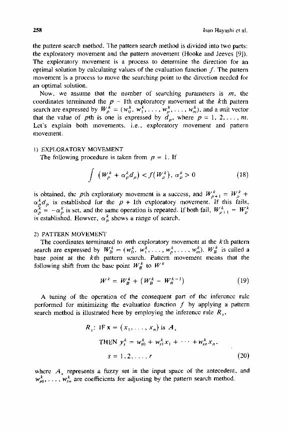
258 Isao Hayashi et al.
the pattern search method. The pattern search method is divided into two parts: the exploratory movement and the pattern movement (Hooke and Jeeves [9]). The exploratory movement is a process to determine the direction for an optimal solution by calculating values of the evaluation function f . The pattern movement is a process to move the searching point to the direction needed for an optimal solution.
Now, we assume that the number of searching parameters is m, the coordinates terminated the p - lth exploratory movement at the kth pattern search are expressed by Wp k = (w0 ~, w~ . . . . . Wp k . . . . . Wmk), and a unit vector that the value of p th is one is expressed by dp, where p = 1, 2 . . . . . m. Let 's explain both movements, i.e., exploratory movement and pattern movement.
1) EXPLORATORY MOVEMENT The following procedure is taken from p = 1. If
f k > o (18) ( Wp k + u~dp) < f (W p k ) , OZp
is obtained, the p th exploratory movement is a success, and Wff+ l = Wff -1- oL~dp is established for the p + Ith exploratory movement. If this fails,
- - c ~ is set, and the same operation is repeated. If both fail, Wff+ l = W~ ~ p - -
k shows a range of search. is established. Howver, ap
2) PATTERN MOVEMENT The coordinates terminated to mth exploratory movement at the kth pattern
search are expressed by W~ = (w0 k, w~ . . . . . wp k . . . . . Wmk). Wff is called a base point at the kth pattern search. Pattern movement means that the following shift from the base point W~ to W k
W X = W~ + ( W ~ - W f f - ' ) (19)
A tuning of the operation of the consequent part of the inference rule performed for minimizing the evaluation function f by applying a pattern search method is illustrated here by employing the inference rule R s,
Rs: IF x = ( x I . . . . . x . ) is A s
THEN y~ = Ws~ + w~x, + " ' " + wf, x , ,
s = 1 ,2 . . . . . r (20)
where A s represents a fuzzy set in the input space of the antecedent, and Wfo . . . . . w~,, are coefficients for adjusting by the pattern search method.

Construction of Fuzzy Inference Rules 259
Given the ith input data X i = ( x , . . . . . x i , , ) , the estimate y* can be derived from the equation
As(x,, . . . . . X,n) X (Wso + ws, x , , + " " +WsnX,n) y , = s = l
r
Z #As(Xi, . . . . . Xin) s = l
i = 1 ,2 . . . . . N (21)
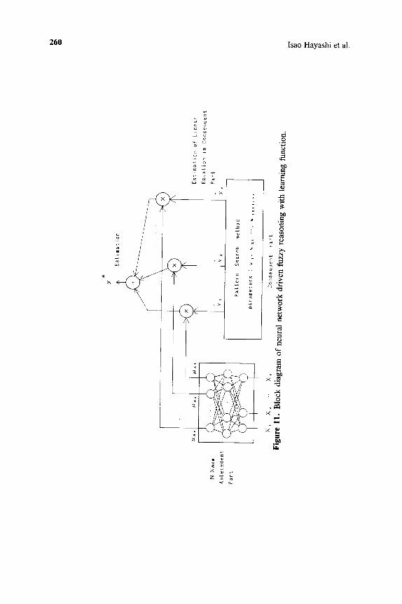
A fundamental structure of this method is shown in Figure 11. This shows that the form of fuzzy set A s of the antecedent is determined by a backpropa- gation type of neural network model NNmem, and a pattern search is made to improve the amount of operation W s o , . . . , wsn for the evaluation function f to attain an optimum value.
The steps of this algorithm are explained below.
STEP 1 Divide input-output data x i = ( X i l , . . . , Xin ) into r classes of R s,
where s = 1 , 2 , . . . , r. The input-output data for each R s are expressed by ( y ~ , x ] ) = (YT , x ] l , x]2 . . . . . x ]n) , where i = 1,2 . . . . . N s, provided that N s is a number of input-output data for each R s. NN . . . . in Figure 11 conducts backpropagation learning in the same way as step 2 of the NDF algorithm. After conducting a backpropagation learning, the estimated value of the output represents the membership value of fuzzy sets A s of each rule.
STEP 2 The initial values W°so, • • - , wOn of the coefficients of equations in the consequent parts required for the search are set.
STEP 3 The kth base point in the pattern search method is represented by (Wo*, w , * , . . * * * . . . . . w,*n, = . , w p . . . . . w m) = ( W l o ,
W2ko, , W~ . . . . . . Wrko . . . . . Wrkn). The kth exploratory movement is taken from W l k = W~.
k is reset STEP 4 If whole exploratory movements fail, an absolute value of C~p to a smaller value. However, if
k I < c (22) max ] C~p = P
is obtained, a procedure of algorithm is terminated, where E is a threshold to stop the algorithm.
STEP 5 The pattern movement from the base point W~ to W k is taken by using Eq. (19). After the pattern movement, the exploratory movement is taken
260 Isao Hayashi et al.
i /
/ r
o
o - c
o
O
~D
N
c ) ,
~D e.,
~D
E
X
o
× . ~

Construction of Fuzzy Inference Rules 261
from WI k = W k, and WB T M = Wm*÷l is set after the exploratory movement.
STEP 6 If
f( W~ +l) < f(Wff) (23) is obtained, go to step 5 as k = k + 1. If it fails, go to step 4.
A N A P P L I C A T I O N TO S E C O N D A R Y F U N C T I O N I D E N T I F I C A T I O N
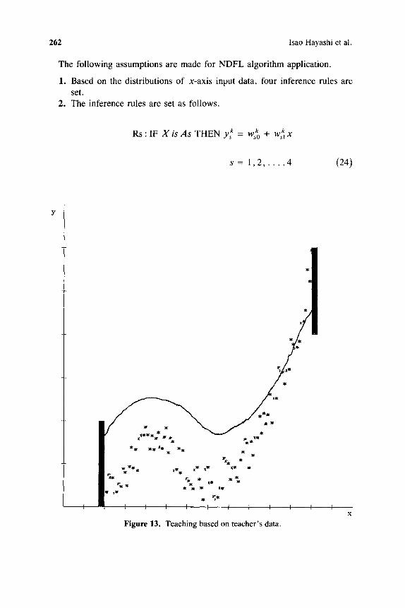
To verify the effectiveness of the NDFL algorithm, an identification of a simple secondary function is conducted for a case where the input-output data are both the input and output of ( x , y ) shown in Figure 12.
X ~
tit
~lt llt~ 11¢ ~ S ~S I ~ 1 t lit
lit )S ~ Z lit ~'~ I~ llg
I , I I i I I I I I t I
Figure 12. Input and output data for secondary function identification.
I X
262 Isao Hayashi et al.
The following assumptions are made for N D F L algorithm application.
1. Based on the distributions of x-axis input data, four inference rules are set.
2. The inference rules are set as follows.
Rs : IF X is As THEN yks = Ws~ + Ws~ x
s = 1 ,2 . . . . . 4 (24)
l i t
j
I l I I I l I I I I
Figure 13. Teaching based on teacher's data.
I x
Construction of Fuzzy Inference Rules 263
3. The neural network for determining the antecedent part of the fuzzy inference rule is set as a three-layer [1 × 5 × 4], and the number of learnings is set at 550.
4. d~ is reduced from 1.0 by using d~ = (1/2) g, g = 0, 1, 2 . . . . . and a threshold ~ is set as ~ = 0.01.
5. The evaluation function f is set as a sum of mean squares of errors between output value and estimated value.
As shown in Figure 13, a teaching based on the teacher's data (x~, y~), where t = 1, 2 . . . . . 25 is made first. The solid line in Figure 13 shows the teaching of the teacher 's data. The initial values wOo, w°t of the coefficients of equations in the consequent parts are derived by using the following set of equations.
Ws°j = ~ - - 4 (25a) =1 X t + I - - X t
wOI = Y t 2 = 1 X t + I - - X s
s = 1 ,2 . . . . . 4, t = 1 ,2 . . . . . 25
where the treacher's data (x~, y , ) are obtained from the solid line in Figure 13. The search is commenced by assigning coefficients derived from the teacher's data to the initial values of search variables of the consequent of the fuzzy inference rule. Figure 14 shows an estimated curve obtained by this search, with reasonable estimated values representing the given input-output data.
The inference rules consequently obtained are
Rt: IF x is A t
THEN Yt = 2 . 0 9 + 2 .87x
R2: IF x is A z
(26a)
THEN Ye = 20.61 - 3 .76x (26b)
R3: IF x is A 3
THEN Y3 = - 1 2 . 1 3 + 3 . 1 2 x (26c)
R4: IF x is A 4
THEN Y4 = - 4 1 . 3 9 + 6 . 8 1 x (26d)
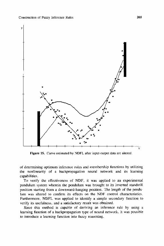
When part of the given input-output data are altered assuming a case where a change is made in the inference environment, NDFL is still applicable for constructing an inference rule. Figure 15 shows an estimated curve obtained by

264
Y
Isao Hayashi et al.
~lglg x lit llllt z
F'igure 14. Curve estimated by NDFL.
NDFL after the input-output data are altered, and also shows a reasonable estimated curve as in the case illustrated in Figure 14.
As shown in the above, NDFL can be used to construct inference rules quickly and precisely even if the environment for constructing an inference rule is dynamically changing.
CONCLUSION
Whereas conventional fuzzy reasoning is associated with inherent tuning problems, NDF and NDFL are, when input-output variables are given, capable
Construction of Fuzzy Inference Rules 265
Y
S
\ ,
Figure 15. Curve estimated by NDFL after input-output data are altered.
of determining optimum inference rules and membership functions by utilizing the nonlinearity of a backpropagation neural network and its learning capabilities.
To verify the effectiveness of NDF, it was applied to an experimental pendulum system wherein the pendulum was brought to its inverted standstill position starting from a downward-hanging position. The length of the pendu- lum was altered to confirm its effects on the NDF control characteristics. Furthermore, NDFL was applied to identify a simple secondary function to verify its usefulness, and a satisfactory result was obtained.
Since this method is capable of deriving an inference rule by using a learning function of a backpropagation type of neural network, it was possible to introduce a learning function into fuzzy reasoning.

266 Isao Hayashi et al.
References
1. Hirota, K., Robotics and automation industrial applications in Japan, 3rd IFSA Congress, Seattle, 229-230, 1989.
2. Lee, C. C., A self-learning rule-based controller with approximate reasoning, Memo No. UCB/ERL, M89/84, Univ. Berkeley, 1989.
3. Hayashi, I., Nomura, H., and Wakami, N., Artificial neural network driven fuzzy control and its application to the learning of inverted pendulum system, 3rd 1FSA Congress, Seattle, 610-613, 1989.
4. Takagi, H., and Hayashi, I., NN-driven fuzzy reasoning, Int. J. Approx. Reasoning, 5(3), 191-212, 1991.
5. Anderson, J., and Rosenfield, E., Neurocomputing, MIT Press, Cambridge, Mass., 1988.
6. Tank, D., and Hopplield, J., Collective computations in neuronlike circuits, Sci. Am. 104-114, 1987.
7. Rumlhart, D. E., Hinton, G. E., and Williams, R. J., Learning representations by backpropagation errors, Nature 323(9), 533-536, 1986.
8. Sugeno, M., and Kang, G. T., Structure identification of fuzzy model, Fuzzy Sets Syst. 28(1), 15-33, 1988.
9. Hooke, R., and Jeeves, T. A., Direct search solution of numerical and statistical problems J, ACM 8, 212-221, 1961.