Constructing new covering arrays from LFSR sequences over finite

fields

Georgios Tzanakisa,∗, Lucia Mourab,, Daniel Panarioa,, Brett Stevensa,

a School of Mathematics and Statistics, Carleton University1125 Colonel By Dr., Ottawa, ON K1S 5B6

b School of Electrical Engineering and Computer Science, University of Ottawa800 King Edward Ave., Ottawa, ON K1K 6N5

Abstract

Let q be a prime power and Fq be the finite field with q elements. A q-ary m-sequenceis a linear recurrence sequence of elements from Fq with the maximum possible period. Acovering array CA(N ; t, k, v) of strength t is a N ×k array with entries from an alphabet ofsize v, with the property that any N×m subarray has at least one row equal to every possiblem-tuple of the alphabet. The covering array number CAN(t, k, v) is the minimum numberN such that a CA(N ; t, k, v) exists. Finding upper bounds for covering array numbers is oneof the most important questions in this research area. Raaphorst, Moura and Stevens givea construction for covering arrays of strength 3 using m-sequences that improves upon someprevious best bounds for covering array numbers. In this paper we introduce a method thatgeneralizes this construction to strengths greater than or equal to 4. Our implementationof this method returned new covering arrays and improved upon 38 previously best knowncovering array numbers. The new covering arrays are given here by listing the essentialelements of their construction.

Keywords: covering arrays, linear feedback shift register sequences, primitive polynomialsover finite fields, exhaustive search algorithms2010 MSC: 94A55, 05B20

1. Introduction

Let M be a N ×k array with entries from an alphabet of size v. If the N × s subarray ofM defined by s columns contains every one of the vs possible s-tuples at least once, then theset of these columns is covered ; otherwise, it is uncovered. If there exists a positive integert ≤ k such that every t columns of M are covered, then M is a covering array of strength tand size N , denoted by CA(N ; t, k, v).

∗Corresponding authorEmail addresses: gtzanaki@math.carleton.ca (Georgios Tzanakis), lucia@eecs.uottawa.ca (Lucia

Moura), daniel@math.carleton.ca (Daniel Panario), brett@math.carleton.ca (Brett Stevens)

Preprint submitted to Discrete Mathematics October 1, 2015

In areas such as software development and manufacturing, it is often infeasible to performexhaustive system tests. However, empirical research shows that in many types of systemserrors are triggered only when a small number of factors interact [18]. In those cases, apractical alternative is t-way combinatorial testing, where the objective is to check everyt-combination of factors. This approach can dramatically reduce the number of tests thatneed to be performed, while still being extremely effective in detecting errors [5, 18]. At-way combinatorial test suite with N tests, for a system with k factors each with v possiblelevels, corresponds to a CA(N ; t, k, v). In this context, the construction of covering arraysof small sizes is important, since it implies a reduction on the number of tests, time and costneeded for a system to be tested.

For given t, k, v, the smallest N such that a CA(N ; t, k, v) exists is the covering arraynumber CAN(t, k, v). Only few families of covering arrays are known that have a minimumnumber of rows [3, 16, 17]. Generally, for fixed t and v, a CA(N ; t, k, v) with N = O(log k)can be constructed in polynomial time [2]. Other upper bounds for covering array numbersfollow from numerous methods for obtaining covering arrays that exist in the literature.These include combinatorial and algebraic constructions [4, 21, 22], greedy [2, 7, 31] andmetaheuristic [6, 14, 25, 30] computer algorithms, and recursive methods for obtaining newcovering arrays from existing ones [7, 10, 11, 15]. Surveys on the subject include [9, 19], and[1, Chapter 3]. Colbourn as of this date actively maintains an online database of the bestknown upper bounds for covering array numbers [8].

Linear Feedback Shift Register (LFSR) sequences over finite fields have been extensivelyused in applications such as cryptography and communications [13, 20], but less so for theconstruction of combinatorial arrays. An orthogonal array OAλ(t, k, v) is a λvt×k array overan alphabet of size v, with the property that the λvt × t subarray defined by any t columnscontains each t-tuple exactly λ times. When λ = 1, we simply write OA(t, k, v); such anarray is also an optimal CA(vt; t, k, v). Munemasa [24] uses LFSR sequences correspondingto primitive trinomials over F2, to create strength-2 binary orthogonal arrays that are veryclose to being strength 3. Raaphorst et al [27] employ LSFR sequences to construct aCA(2q3 − 1; 3, q2 + q + 1, q) for every prime power q. This is, to the best of our knowledge,the only construction in the literature that uses LFSR sequences to construct covering arraysthat are not orthogonal arrays.

In this paper, we introduce a method of using LFSR sequences to build covering arraysbased on theoretical results established in [27]. It yields covering arrays over finite fieldswith q elements, strength t, and size l(qt − 1) + 1, where q is a prime power, and l, t areintegers with l ≥ 1, t ≥ 2. It generalizes two of the previous LFSR-based constructions; fort = 2, our method yields an OA(2, q + 1, q), and for t = 3 the covering arrays in [27]. Forthe implementation of our method, we give algorithms that rely on finite field theory andcombinatorial exhaustive generation. In particular, we use backtracking for this generationand reduce the search space by proving finite field properties and by using generation ofbinary necklaces. Finally, we discuss our implementation which gave 38 new covering arraysthat improve upon previously best upper bounds for covering array numbers of strength 4,found in [8].

The structure of this paper is as follows. In Section 2 we give some background on

2

LFSR sequences, we discuss how they are used to construct covering arrays, and we givean overview of our method. The method relies on two parts, to which we dedicate Sections3 and 4. In Section 5 we discuss our computer implementation of the method and presentour results. In Section 6 we conclude with some remarks on connections of our method withfinite geometry.

2. LFSR sequences and arrays

2.1. Preliminaries

We begin with some background on LFSR sequences; for a comprehensive presentationwe refer to [13] and [20, Chapter 5].

Let f(x) = xm + cm−1xm−1 + · · ·+ c1x+ c0 ∈ Fqm [x], and I = (b0, . . . , bm−1) ∈ Fqm . The

sequence S(f, I) = (a0, a1, . . . ) defined as

ai =

{bi if 0 ≤ i < m,

−cm−1ai−1 − cm−2ai−2 − · · · − c1ai−(m−1) − c0ai−m if i ≥ m,(1)

is an LFSR sequence over Fq with characteristic polynomial f and initial values I. For everysuch sequence there exists a positive integer P such that ai = aP+i; the smallest such P isthe least period of the sequence, and it divides qm − 1.

Suppose that f is irreducible, α ∈ Fqm is one of its roots, and furthermore α generatesthe multiplicative group F∗qm = Fqm \ {0} of Fqm . Then α is a primitive element of Fqm , andf is a primitive polynomial. An LFSR sequence with primitive characteristic polynomial isan m-sequence, that is, a sequence with period qm − 1, which is maximum.

The trace function in Fqm over Fq is the mapping

Trqm/q : Fqm −→ Fqx 7→ x+ xq + xq

2

+ xq3

+ · · ·+ xqm−1

,

which is linear over Fq, i.e. Trqm/q(ca+ b) = cTrqm/q(a) + Trqm/q(b) for all c ∈ Fq, a, b ∈ Fqm .The trace is used to represent m-sequences as follows.

Proposition 2.1 ([20, Theorem 8.33]). Let f be a primitive polynomial over Fq of degree mand α ∈ Fqm one of its roots. For any initial values I = (a0, . . . , am−1) there exists a uniqueelement β ∈ Fqm such that bi = Tr(βαi) for all 0 ≤ i ≤ m − 1. Then, the LFSR sequenceS(f, I) = (a0, a1, . . . ) has the property that ai = Tr(βαi), for all i ≥ 0.

In Proposition 2.1, the sequence(Trqm/q(βα

i))i≥0

is the trace representation of S(f, T ).

If β = αs for some s, then(Trqm/q(βα

i))i≥0

is the left cyclic shift of (Tr(αi))i≥0 by s. In this

paper, we refer to(Trqm/q(α

i))i≥0

as the LFSR sequence associated with α.

Let α be a primitive element of Fqm , w = (qm − 1)/(q − 1), and a = (ai)i≥0 be theLFSR sequence associated with α. We denote the left cyclic shift by i of a as Lwi (a) =(ai, ai+1, . . . , ai+w−1), and define

3

M(α) =

Lw0 (a)Lw1 (a)

...Lwqm−2 (a)0, 0, . . . , 0

. (2)

We note that for 0 ≤ i ≤ qm−2, 0 ≤ j ≤ w−1, the (i, j)-th element of M(α) is Trqm/q(αiαj).

The following theorem describes the coverage properties of M(α), and is the cornerstoneof the results of this paper.

Theorem 2.2 (See [27, Theorem 2]). Let q be a prime power, α be a primitive element ofFqm, m ≥ 3, w = (qm − 1)/(q − 1), and c0, c1, . . . , cw−1 denote the column vectors of M(α).Then, the following are equivalent.

1. A set of columns {ci1 , . . . , cis} is uncovered in M(α).

2. The elements αi1 , . . . , αis ∈ Fqm are linearly dependent over Fq.

Furthermore, if s = m the following is also equivalent to (1) and (2).

3. There is a row r other than the all-zero, such that ri1 = · · · = rim = 0.

Let q be any prime power, α be a primitive element of Fq3 , and let M ′(α) be the arraythat consists of the columns of M(α) in reverse order. Raaphorst et al [27] prove that thevertical concatenation of M(α), M ′(α), and a row of zeros, is a CA(2q3− 1; 3, q2 + q+ 1, q).The same construction for m > 3 does not yield a covering array, so it is natural to askwhether a different generalization can be given.

Observing that reversing the columns of the matrix can be considered as a permutationof its columns, the authors of [27] considered the following generalized construction. Theygenerated M(α) for primitive α ∈ Fqm , m ≥ 4, and ran search algorithms to find a permuta-tion group of smallest order s(m, q), such that vertically concatenating the s(m, q) permutedcopies of M(α) and a row of zeros, yields a CA(s(m, q)(qm − 1) + 1;m, (qm − 1)/(q − 1), q).The resulting arrays in those attempts did not improve the known best upper bounds forcovering array numbers.

We note that when α ∈ Fqm is primitive then so is α−1, and M ′(α) = M(α−1). With thatin mind, in this paper we consider the following generalization. Let α1, . . . , αl be primitiveelements of Fqm , and w = (qm−1)/(q−1). We define the LFSR array generated by α1, . . . , αl,denoted M(α1, . . . , αl), to be the vertical concatenation of M(α1), . . . ,M(αl) with all butone copy of the all-zero rows removed. We note that M(α1, . . . , αl) is a (l(qm − 1) + 1)×warray.

Special cases of LFSR arrays have been previously used to produce covering and orthog-onal arrays:

4

• For any m ≥ 2, any prime power q, and primitive α ∈ Fqm , we have that M(α) isan OAλ(2, (q

m − 1)/(q − 1), q) with λ = qm−1. This follows from the 2-tuple balanceproperty of m-sequences (see [13, Section 5.6]).

• For m = 3, any prime power q, and primitive α ∈ Fqm , from [27] we have thatM(α, α−1) is a CA(2(q3 − 1) + 1; 3, q2 + q + 1, q).

• We have from [12] that for α ∈ Fm2 whose minimal polynomial is a pentanomial thatsatisfies certain conditions, the array consisting of 2m consecutive columns of M(α) isa OAλ(3, 2m, 2), with λ = 2m−3, which is a CA(2m; 3, 2m, 2). This is an extension ofa result by Munemasa [24].

• We have from [26] that for α ∈ Fm3 whose minimal polynomial is a trinomial thatsatisfies certain conditions, any array consisting of 3m consecutive columns of M(α)is a OAλ(3, 3m, 3), with λ = 3m−3. This is also a CA(3m; 3, 3m, 3).

2.2. A new method for constructing covering arrays from LFSR sequences

For integers i, j with i < j we denote [i, j] = {i, i+ 1, . . . , j}.Let M be an N × k array with columns c0, . . . , ck−1, and let e ⊆ [0, k − 1]. We define

M [e] to be the subarray of M consisting of the columns ci, i ∈ e. The following methodyields covering subarrays of LFSR arrays.

Method 1 (Covering arrays from LFSR arrays). Let q be a prime power and m ≥ 3. Thefollowing steps yield a covering array of strength m over Fq.

Step 1: Choose primitive elements α1, . . . , αl ∈ Fqm for some l ≥ 2, and construct M =M(α1, . . . αl).

Step 2: Find a subset e of column indices of M with maximum size, such that M [e] is acovering array.

The array M [e] is a CA(l(qm − 1) + 1;m, |e|, q).

In the following sections we discuss algorithms to efficiently implement this method. InSection 3 we determine how to choose the primitive elements in Step 1 so that we avoidredundancies, and in Section 4 we give an algorithm that solves the optimization problemin Step 2.

3. The choice of primitive elements

A question that naturally arises from the description of Method 1 is what should thechoice of α1, . . . , αl be in Step 1, so that the resulting covering array in Step 2 has the

5

maximum number of columns. It is well known (see for example [13, Theorem 4.9] ) thatthere exist Φ(qm − 1)/m shift-distinct m-sequences of order m over Fq, so this is also thenumber of different LFSR arrays. Hence, a straightforward approach would be to carryout the method for all

(Φ(qm−1)/m

l

)l-tuples of elements α1, . . . , αl that correspond to those

distinct m-sequences.Let w = (qm − 1)/(q − 1), and q = pn for a prime p and positive integer n. In this

section we use finite fields to partition the set of all primitive elements of Fqm into Φ(w/mn)classes, with the property that two primitive elements are in the same class if and only ifthey correspond to LFSR arrays with identical coverage of columns. It follows that we onlyneed to choose one representative from each of those classes, and carry out the method forthe

(Φ(w/mn)

l

)l-tuples α1, . . . , αl of representatives.

The above-mentioned classes use the notion of cyclotomic cosets. For i ∈ Z∗w, we definethe cyclotomic coset of p modulo w that contains i to be the set

Cip,w = {ipr (mod w) : r ∈ Z≥0} .

For any i, j ∈ Z∗w, we have that Cip,w ⊆ Z∗w and, furthermore, if Ci

p,w ∩ Cjp,w 6= ∅ then

Cip,w = Cj

p,w. We conclude that there exists a set Γp,w ⊆ Z∗w such that

Z∗w =⋃

i∈Γp,w

Cip,w, (3)

and for all i, j ∈ Γp,w with i 6= j, we have that Cip,w ∩Cj

p,w = ∅. The elements of Γp,w are thecyclotomic coset leaders of p modulo w.

Definition 3.1. Let m ≥ 2, and M1, M2 be N × k arrays with elements from an alphabetof the same finite size. Denote ci, di, i ∈ [0, k − 1] to be their columns, respectively. Thearrays M1 and M2 have the same m-coverage if for every I ⊆ [0, k − 1] with |I| = m, wehave that {ci : i ∈ I} is covered if and only if {di : i ∈ I} is covered.

The main theoretical result of this section is the following.

Theorem 3.2. Let q be a power of a prime p, and m,w be integers with m ≥ 2, w =(qm − 1)/(q − 1). Let α be a primitive element of Fqm. Then for any i ∈ Γp,w we have thatαi is also a primitive element of Fqm, and the following hold.

1. For any primitive element β ∈ Fqm, there exists i ∈ Γp,w such that M(β) and M(αi)have the same m-coverage.

2. For all i, j ∈ Γp,w with i 6= j, we have that M(αi) and M(αj) do not have the samem-coverage.

The proof of Theorem 3.2 requires several theoretical results that we give later in thesection. First we discuss its implications regarding Method 1. In particular, it follows fromTheorem 3.2 that it suffices to carry out Method 1 only for l-tuples of primitive elementsαi1 , . . . , αil where {i1, . . . , il} ∈

(Γp,w

l

). From the next proposition we have that |Γp,w| = Φ(w)

mn,

hence we have(

Φ(w)/mnl

)l-tuples of primitive elements to examine.

6

Proposition 3.3. Let p be a prime, and n, q,m,w be integers with n > 0, q = pn, m ≥ 2,w = (qm − 1)/(q − 1). Then we have that |Ci

p,w| = mn, for all i ∈ Z∗w.

Proof. The size of Cip,w is equal to the smallest positive integer r such that ipr ≡ i (mod w),

which is equivalent to w|pr − 1, since gcd(i, w) = 1. Now, w|qm − 1 = pmn − 1, and thuspmn ≡ 1 (mod w). We note that, by its definition, r is the order of p in Z∗w and thereforepmn ≡ 1 (mod w) implies that r|mn, hence r ≤ mn. Assume by means of contradiction thatr < mn. Then, since r|mn, it must be r ≤ mn/2. On the other hand, since w|pr−1, we havethat pr − 1 ≥ w > pmn−n− 1, and thus r > mn− n. Then mn/2 > mn− n which simplifiesto m < 2, contradicting our assumption that m ≥ 2. We conclude that r = mn.

The rest of the section is dedicated to the proof of Theorem 3.2. First, we need to provea few auxiliary lemmas.

Lemma 3.4. Let q be a prime power, m be an integer with m ≥ 2, and α, β primitiveelements of Fqm. Then, M(α) and M(β) have the same m-coverage if and only if thereexists γ ∈ Fqm such that, for all s ∈ [0, qm − 2],

Trqm/q(αs) = 0 if and only if Trqm/q(γβ

s) = 0.

Proof. Let w = (qm − 1)/(q − 1) and {a0, . . . , aw−1}, {b0, . . . , bw−1} be the column vectorsof M(α) and M(β) respectively.

“⇐” Let I ⊆ [0, w − 1] such that |I| = m and {ai : i ∈ I} is covered. Suppose bycontradiction that {bi : i ∈ I} is uncovered. Then, by Theorem 2.2 there exists a row ofM(β) that has zeros at the columns bi, i ∈ I. From the definition of M(β), the lattermeans that there exists γ ∈ F∗qm such that Trqm/q(γβ

i) = 0 for all i ∈ I. This implies thatTrqm/q(α

i) = 0 for all i ∈ I, which means that {ai : i ∈ I} is uncovered, a contradiction.“⇒” We observe that ord(αw) = q − 1, hence αw is a primitive element of F∗q, and for

every s ∈ [0, qm − 2] we have that αs = cαu, where u ∈ [0, w − 1], u ≡ s (mod w), andc ∈ Fq. Hence, from the linearity of the trace over Fq, it is sufficient to prove this directionfor all s ∈ [0, w − 1].

We know that ker(Trqm/q) is a vector space over Fq with dimension m − 1 (see forexample [23, Theorem 2.1.83]). Since α is primitive, it follows from the above that thereexist i1, . . . , im−1 ∈ [0, w − 1] such that B = {αi1 , . . . , αim−1} is also a basis for ker(Trqm/q).This means that αi1 , . . . , αim−1 are linearly independent and the first row of M(α) has zerosat the columns ai, i ∈ {i1, . . . , im−1}. Then, from Theorem 2.2 and our assumption thatM(α) and M(β) have the same m-coverage, βi1 , . . . , βim−1 are also linearly independent,and there exists a row of M(β) with zeros at the columns bi, i ∈ {i1, . . . , im−1}. The lattermeans that there exists γ ∈ F∗qm such that Trqm/q(γβ

i) = 0 for all i ∈ {i1, . . . , im−1}. Weconclude that B′ = {γβi1 , . . . , γβim−1} is a basis for ker(Trqm/q).

Now, suppose that Trqm/q(αs) = 0 for some s ∈ [0, w − 1]. Then, by Theorem 2.2,

we have that the set of columns{ai1 , . . . , aim−1 , as

}of M(α) is uncovered and thus the set

of columns{bi1 , . . . , bim−1 , bs

}of M(β) is also uncovered, from our assumption that M(α)

and M(β) have the same m-coverage. Hence there exists a row of M(β) with zeros at the

7

columns bi1 , . . . , bim−1 , bs, and so there exists δ ∈ F∗qm such that δβi ∈ ker(Trqm/q) for alli ∈ {i1, . . . , im−1, s}. Since B′ is a basis for ker(Trqm/q), we have that δ = cγ for some c ∈ F∗q.Then δβs ∈ ker(Trqm/q) implies that γβs ∈ ker(Trqm/q) from the linearity of the trace.

Lemma 3.5. Let p be a prime, and q, n,m, l integers with n > 0, q = pn, m ≥ 2, and0 < l < qm − 1. Then, we have that Trqm/q(x

l) = Trqm/q(x)l for all x ∈ Fqm if and only ifl = pr for some integer r such that 0 ≤ r < mn.

Proof. If l = pr, 0 ≤ r < mn, then Trqm/q(xl) = Trqm/q(x)l from the properties of the

Frobenius automorphism in Fq.Conversely, suppose that Trqm/q(x

l) = Trqm/q(x)l for all x ∈ Fqm . For a polynomial f onx, we denote [xn]f(x) to be the coefficient of xn in f . We observe that

[x1+(l−1)q]Trqm/q(xl) =

{1, if l = 1

0, otherwise,(4)

and

[x1+(l−1)q]Trqm/q(x)l =

{1, if l = 1

l, otherwise.(5)

If l = 1, then l = pr with r = 0. If l > 1, then it follows from Equations (4) and (5) andour assumption that Trqm/q(x

l) = Trqm/q(x)l, that l ≡ 0 (mod p). Hence l = kpr for somepositive integers k, r, with 0 < r < mn, and p 6 | k. We have that, for all x ∈ Fqm ,

Trqm/q(xk)p

r

= Trqm/q(xkpr) = Trqm/q(x

l) = Trqm/q(x)l

=(Trqm/q(x)k

)pr. (6)

Taking pr-th roots in Equation (6) yields that Trqm/q(xk) = Trqm/q(x)k for all x ∈ Fqm .

By comparing the coefficients of Trqm/q(xk) and Trqm/q(x)k in the same way as we did for

Trqm/q(xl) and Trqm/q(x)l, we have that either k = 1, or k ≡ 0 (mod p). Since we have

assumed that p 6 | k, it must be k = 1, and thus l = pr.

Lemma 3.6. Let p be a prime, q, n,m be integers such that n > 0, q = pn, m ≥ 2, andα, β primitive elements of Fqm. Then M(α) and M(β) have the same coverage if and onlyif β = αp

r, for some r ∈ [0,mn− 1].

Proof. If β = αpr

for some r ∈ [0,mn−1], then for every s ∈ [0, qm−2] we have Trqm/q(βs) =

Trqm/q(αspr) = Trqm/q(α

s)pr. Hence, Trqm/q(β

s) = 0 if and only if Trqm/q(αs) = 0, and thus

M(α) and M(β) have the same m-coverage, from Lemma 3.4.For the converse, assume that M(α) and M(β) have the same m-coverage. Since α

is primitive, there exists l ∈ Z∗qm−1 such that β = αl. Then, from Lemma 3.4, thereexists γ ∈ Fqm such that, for all s ∈ [0, qm − 2], we have Trqm/q(α

s) = 0 if and only ifTrqm/q(γα

ls) = 0. Again from the primitivity of α, we have that F∗qm = {αs : s ∈ [0, qm − 2]},so we conclude from the above that there exists γ ∈ Fqm such that, for all x ∈ F∗qm , we have

Trqm/q(x) = 0 if and only if Trqm/q(γxl) = 0. (7)

8

Let y be an element of some extension of Fqm such that Trqm/q(γyl) = 0. Then γyl =

z ∈ ker(Trqm/q) ⊆ Fqm , and yl = z/γ ∈ Fqm . Since gcd(l, qm − 1) = 1, the l-th root of z/γexists, and y = (z/γ)1/l ∈ Fqm . We have proved that Trqm/q(γx

l) splits in Fqm . Now,

Trqm/q(γxl) =

∏a∈ker (Trqm/q)

(γxl − a

).

Because Trqm/q(γxl) splits in Fqm , so does γxl − a for all a ∈ ker(Trqm/q). Furthermore, the

only root of γxl − a is (a/γ)1/l, and its degree is l; it follows that it must be γxl − a =γ(x− (a/γ)1/l)l, and so

Trqm/q(γxl) =

∏a∈ker (Trqm/q)

γ(x− (a/γ)1/l)l. (8)

From Equation (7) we have that

ker(Trqm/q) ={

(a/γ)1/l ; a ∈ ker(Trqm/q)},

and it is well known that | ker(Trqm/q)| = qm−1, hence Equation (8) becomes

Trqm/q(γxl) = γq

m−1∏

a∈ker(Trqm/q)

(x− a)l

= γqm−1

∏a∈ker(Trqm/q)

(x− a)

l

= γqm−1

Trqm/q(x)l. (9)

By comparing the coefficient of xl in Trqm/q(γxl) and γq

m−1Trqm/q(x)l, we have that γ =

γqm−1

, which means that γ ∈ Fqm−1 . However γ ∈ Fqm , hence γ ∈ Fqm ∩ Fqm−1 = Fq, andfrom the linearity of the trace over Fq, Trqm/q(γx

l) = γTrqm/q(xl). Equation (9) then implies

that Trqm/q(xl) = Trqm/q(x)l, and by Lemma 3.5 we have that l = pr, for some integer r such

that 0 ≤ r < mn.

Lemma 3.7. Let p be prime, and q, n,m integers with n > 0, q = pn, and w = (qm−1)/(q−1). For all i, j ∈ Z∗qm−1, we have that M(αi) and M(αj) have the same m-coverage if andonly if j (mod w) ∈ Ci

p,w.

Proof. Suppose that j (mod w) ∈ Cip,w. Then there exist integers r, h such that j = ipr+hw,

and thus αj = cαipr

with c = αwh. We have that cq−1 = αw(q−1)h = α(qm−1)h = 1, whichmeans that c ∈ Fq. Then, from the linearity of the trace and the properties of the Frobeniusautomorphism we have that, for all positive integers s,

Trqm/q(αjs) = Trqm/q(c

sαispr

) = csTrqm/q(αis)p

r

.

9

We conclude that Trqm/q(αjs) = 0 if and only if Trqm/q(α

is) = 0, which implies from Lemma3.4 that M(αi) and M(αj) have the same m-coverage.

Conversely, assume that M(αi) and M(αj) have the same m-coverage. Then, fromLemma 3.6 we have that αj = αip

rfor some r ∈ [0,mn− 1], and thus j ≡ ipr (mod qm− 1).

Since w|qm − 1, we also have j ≡ ipr (mod w), which means that j (mod w) ∈ Cip,w.

We now have the background to give the proof of the main theorem.

Proof of Theorem 3.2. We begin with the first part. Let β be a primitive element of Fqm .From the primitivity of α, we have that there exists l ∈ Z∗qm−1 such that β = αl. Let u = l(mod w). Then u = l + hw for some integer h, and thus αu = cαl, with c = αhw. Wehave that cq = c, which means that c ∈ Fq. Hence, for any positive integer s, we havethat Trqm/q(α

us) = csTrqm/q(αls) and therefore Trqm/q(α

ls) = 0 if and only if Trqm/q(αus) =

0. It follows from Lemma 3.4 that M(αl) and M(αu) have the same coverage. Sincegcd(l, qm − 1) = 1, then also gcd(l, w) = 1, hence gcd(u,w) = 1 as well. This means u ∈ Z∗wand thus, from Equation (3), there exists i ∈ Γp,w such that u ∈ Ci

p,w. From Lemma 3.7,M(αu) has the same coverage with M(αi). Since M(αu) was shown above to also have thesame coverage as M(β), we conclude that M(β) has the same coverage with M(αi).

We now prove the second part. Suppose by means of contradiction that i, j ∈ Γp,w,i 6= j, and M(αi) has the same m-coverage with M(αj). Then, from Lemma 3.7 we havethat j ∈ Ci

p,w. Thus, Cip,w ∩Cj

p,w 6= ∅ which means that Cip,w = Cj

p,w, as discussed just beforeEquation (3). This contradicts our assumption that i, j ∈ Γp,w, and we conclude that M(αi)and M(αj) do not have the same coverage.

We close this section by showing how Theorem 3.2 can be used with Method 1. Forprime power q, m ≥ 3, and l ≥ 2, a CA(l(qm − 1) + 1;m, k, q) can be found as follows:

1. Create a set Γp,w of cyclotomic coset leaders modulo w, as defined in Equation (3).This can be done by calculating the cosets Ci

p,w for all i ∈ Z∗w, and picking (any) onerepresentative from each distinct coset.

2. Pick any primitive polynomial Fq[x] and let α be any of its roots.

3. For every {i1, . . . , il} ∈(

Γp,w

l

), find a subset e of column indices of M = M(αi1 , . . . , αil)

with maximum size, such that M [e] is a covering array; see Method 1.

4. Let ({i∗1, . . . , i∗l }, e∗) be a pair ({i1, . . . , il}, e) found in Step 3, where e is maximumamong all such pairs. We have that M(αi

∗1 , . . . , αi

∗l )[e∗] is the desired CA(l(qm − 1) +

1;m, k, q), with |k| = |e∗|.

We note that in Step 2 a different root would produce identical arrays in Step 3. Indeed,for a different root β, we have that β = αq

r, for some r ∈ [0,m − 1] (see [20, Chapter 3]).

Hence, for any i we have Trqm/q(βi) = Trqm/q(α

iqr) = Trqm/q(αi)q

r= Trqm/q(α

i), where thelast equality comes from the fact that Trqm/q(α

i) ∈ Fq. It follows that M(α) = M(β).

10

4. The search for maximum covering subarrays

Step 2 of Method 1 is an optimization problem whose search space consists of sets ofpositive integers. In this section we give an algorithm for Step 2. In Section 4.1 we showhow the search space can be reduced significantly and generated efficiently, and in Section4.2 we present a backtracking algorithm to implement Step 2 of Method 1.

4.1. The search space

We begin by introducing a concept required in this section.

Definition 4.1. For S ⊆ [0, n− 1] and integer i, we define the shift of S by i modulo n tobe

S +n i = {s+ i (mod n) : s ∈ S} .

The next proposition follows from the cyclic nature of LFSR arrays. It can be used toreduce the search space in Step 2 of Method 1.

Proposition 4.2. Let q be a prime power, m ≥ 2, w = (qm − 1)/(q − 1), and α be aprimitive element of Fqm. Denote by c0, c1, . . . , cw−1 the column vectors of M(α) and letS ⊆ [0, w − 1]. Then, for any i ∈ [0, w − 1], we have that {cj : j ∈ S} is covered if and onlyif {cj : j ∈ S +w i} is covered.

Proof. Assume that {cj : j ∈ S} is not covered. From Theorem 2.2 there exists integer rwith 0 ≤ r < qm − 1 such that the row with index r in M(α) has zeros at the columns withindices from S. From the definition of M(α) this means that Trqm/q(α

rαs) = 0 for all s ∈ S.For every j ∈ S +w i we have that j = s + i + kw for some integer k and some s ∈ S.

Setting c = αkw and observing that c ∈ Fq, we have that Trqm/q(αr−iαj) = Trqm/q(cα

rαs) =cTrqm/q(α

rαs) = 0. This shows that the row of M(α) with index r − i (mod qm − 1) haszeros at the columns with indices from S+w i, and using Theorem 2.2, we conclude that theset of these columns is not covered.

It follows from Proposition 4.2 that it is enough to generate subsets of columns of LFSRarrays that are unique up to cyclic shifts. In Section 4.1.1 we establish a criterion for setsto be unique in this sense using binary necklaces, and in Section 4.1.2 we give an algorithmthat generates those unique sets efficiently.

4.1.1. A canonicity criterion for sets

We consider two sets S, T ⊆ [0, n− 1] to be isomorphic if there exists integer i such thatT = S+n i, and we denote ES the equivalence class of S under this isomorphism. We use thenotion of binary necklaces to define canonical representatives of those equivalence classes.

Definition 4.3. Let A be an ordered set and a be a string of elements of A. The necklaceof a, denoted by neck(a), is the lexicographically smallest of all cyclic shifts of a.

In this paper we are only interested in binary necklaces, i.e. A = F2.

11

Example 4.4. Let a = 10101. The following are all the cyclic shifts of a, listed in lexico-graphical order:

01011 < 01101 < 10101 < 10110 < 11010,

therefore, neck(a) = 01011. Let b = 101010. All the (distinct) shifts of b are 010101 and101010, so neck(b) = 010101.

For S ⊂ [0, n−1], we define the characteristic vector of S to be charn(S) = b0b1 · · · bn−1 ∈Fn2 with bi = 1 if and only if i ∈ S. For a binary string b = b0 · · · bn−1 we denote Li(b) =bi · · · bn−1b0 · · · bi−1 its left cyclic shift by i. Finally, the all-zero binary string of length r isdenoted 0r. We also introduce the following binary representation for sets.

Definition 4.5. Let n be a positive integer, S a nonempty subset of [0, n− 1], and considerbi ∈ F2 with 0 ≤ i ≤ max(S), such that bi = 1 if and only if i ∈ S. We define

binn(S) = 0n−max(S)−1b0 · · · bmax(S) ∈ Fn2= Lmax(S)+1(charn(S)).

Moreover, for S = ∅, we define binn(S) = 0n.

In this paper we select canonical representatives of the above-mentioned equivalenceclasses as given in the next definition.

Definition 4.6. A set S ⊆ [0, n−1] is canonical if either S = ∅, or S contains 0 and binn(S)is a necklace.

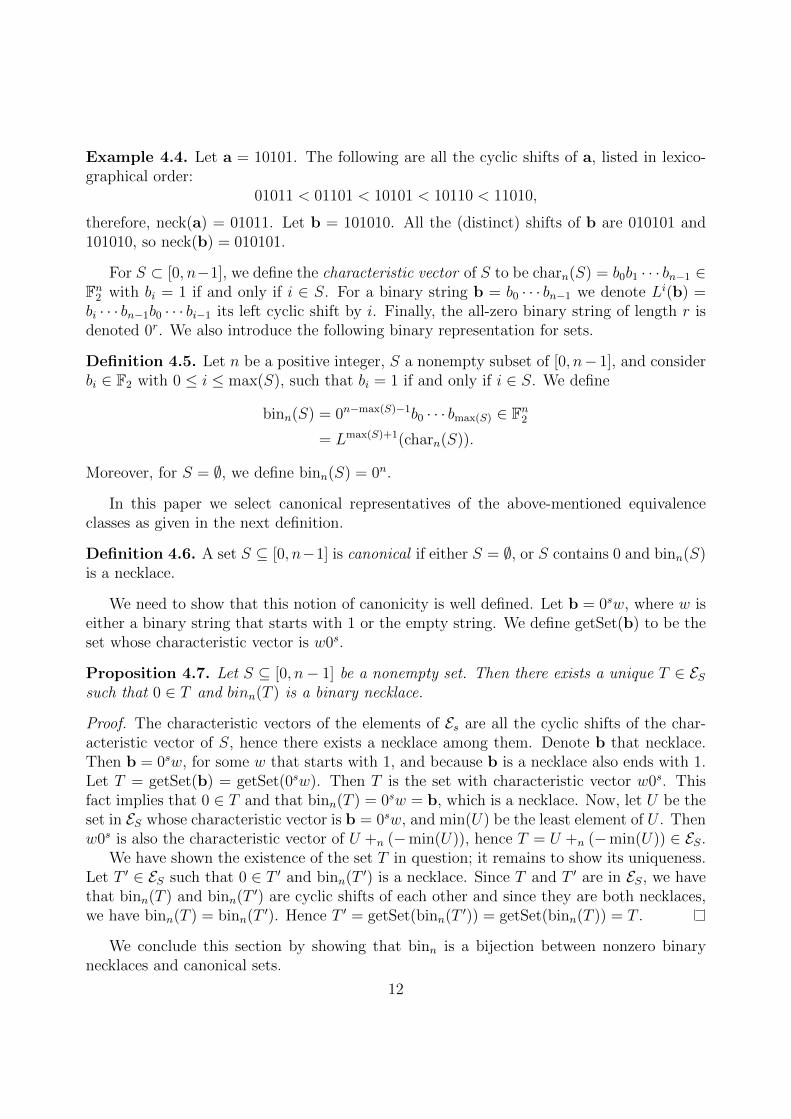
We need to show that this notion of canonicity is well defined. Let b = 0sw, where w iseither a binary string that starts with 1 or the empty string. We define getSet(b) to be theset whose characteristic vector is w0s.

Proposition 4.7. Let S ⊆ [0, n− 1] be a nonempty set. Then there exists a unique T ∈ ESsuch that 0 ∈ T and binn(T ) is a binary necklace.

Proof. The characteristic vectors of the elements of Es are all the cyclic shifts of the char-acteristic vector of S, hence there exists a necklace among them. Denote b that necklace.Then b = 0sw, for some w that starts with 1, and because b is a necklace also ends with 1.Let T = getSet(b) = getSet(0sw). Then T is the set with characteristic vector w0s. Thisfact implies that 0 ∈ T and that binn(T ) = 0sw = b, which is a necklace. Now, let U be theset in ES whose characteristic vector is b = 0sw, and min(U) be the least element of U . Thenw0s is also the characteristic vector of U +n (−min(U)), hence T = U +n (−min(U)) ∈ ES.

We have shown the existence of the set T in question; it remains to show its uniqueness.Let T ′ ∈ ES such that 0 ∈ T ′ and binn(T ′) is a necklace. Since T and T ′ are in ES, we havethat binn(T ) and binn(T ′) are cyclic shifts of each other and since they are both necklaces,we have binn(T ) = binn(T ′). Hence T ′ = getSet(binn(T ′)) = getSet(binn(T )) = T .

We conclude this section by showing that binn is a bijection between nonzero binarynecklaces and canonical sets.

12

Proposition 4.8. There exists a one-to-one correspondence between canonical subsets of[0, n− 1] and binary necklaces of length n.

Proof. We claim that binn is the needed bijection and getSet is its inverse. For S = ∅ wehave binn(S) = 0n and getSet(0n) = ∅ = S.

Let S ⊆ [0, n − 1] be canonical and nonempty. Then by the definition of canonicity,binn(S) is a nonzero necklace of length n. Hence binn maps canonical sets to nonzero binarynecklaces of length n.

Let b be a nonzero binary necklace of length n. Then b = 0sw, 0 ≤ s < n− 1 for somew starting with 1. Let T = getSet(b). Then T has characteristic vector w0s, hence 0 ∈ T .Furthermore binn(T ) = b, a necklace. We conclude that getSet maps binary necklaces tocanonical sets, and it is the inverse of binn when that is restricted to canonical sets.

4.1.2. Generating canonical subsets

Algorithm 1 Generating all nonzero binary necklaces of length n [28].

procedure BinaryNecklaces(b)Output bdone← falsewhile not done do

b← L(b)b′ ← τ(b)if b′ is a necklace then

BinaryNecklaces(b′)else

done← trueMain;BinaryNecklaces(0n−11)

In this section we use the correspondence between canonical sets and binary necklacesto efficiently generate all canonical subsets of [0, n− 1].

For a binary string b = b0 · · · bn−1 we denote τ(b) = b0 · · · bn−2bn−1, where bn−1 is thebinary complement of bn−1. Algorithm 1 above is from Ruskey et al [28]; it generatesevery nonzero binary necklace exactly once. An important feature of this generation is thatonce a non-necklace is encountered, the algorithm backtracks. Thus each time a necklace isgenerated, exactly one non-necklace is examined, therefore yielding a very efficient algorithm,which requires on average only two “necklace checks” for each necklace generated. In orderto generate canonical sets, we translate Algorithm 1 to the language of sets. The next lemmais key to this translation.

Lemma 4.9. Let S ⊆ [0, n − 1] be a nonempty set. Then, for all integers j with 1 ≤ j <n−max(S), we have that binn(S ∪ {max(S) + j}) = τ (Lj(binn(S))).

13

Proof. Let b = binn(S) = 0n−max(S)−1b0 · · · bmax(S), where bi ∈ F2 and bi = 1 if andonly if i ∈ S. Then for integer j with 1 ≤ j < n − max(S), we have τ (Lj(S)) =0n−(max(S)+j)−1b0 · · · bmax(S)0

j−11 = binn(S ∪ {max(S) + j}).

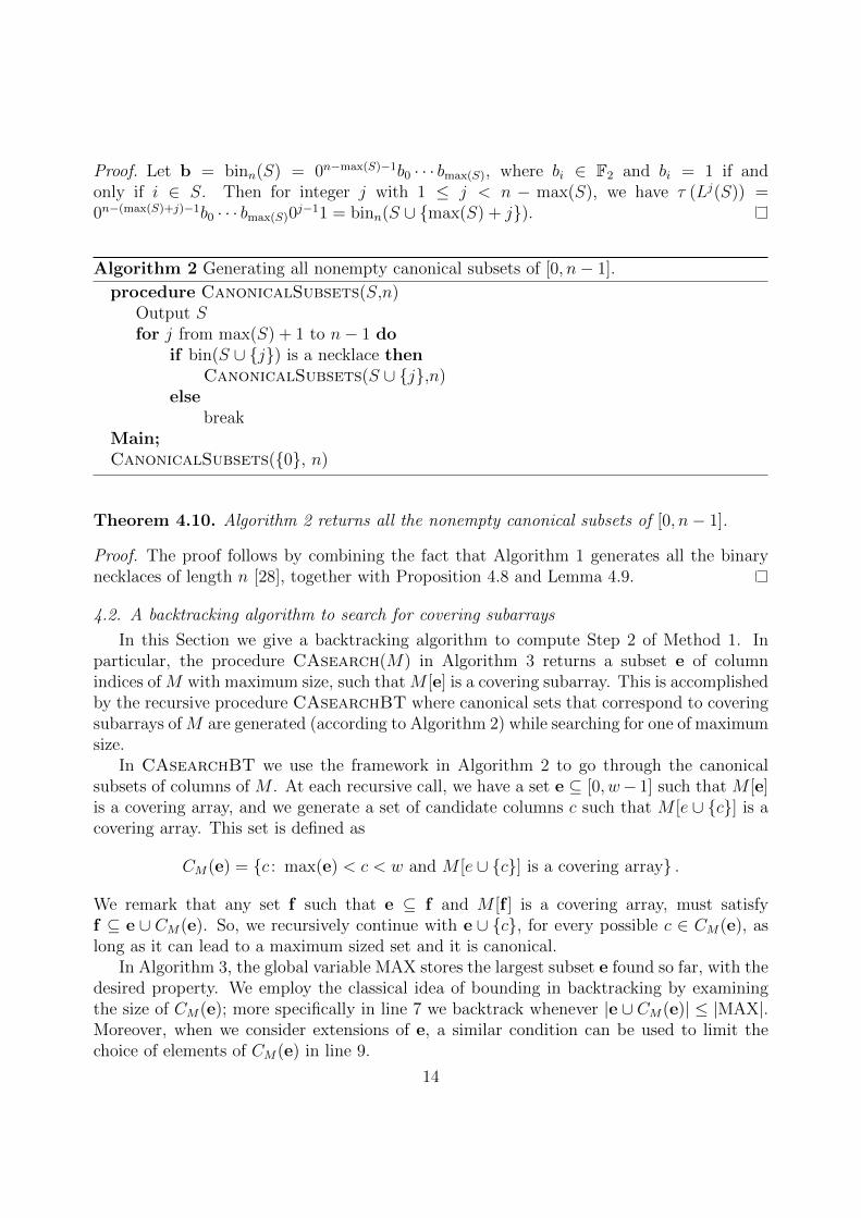
Algorithm 2 Generating all nonempty canonical subsets of [0, n− 1].

procedure CanonicalSubsets(S,n)Output Sfor j from max(S) + 1 to n− 1 do

if bin(S ∪ {j}) is a necklace thenCanonicalSubsets(S ∪ {j},n)

elsebreak

Main;CanonicalSubsets({0}, n)

Theorem 4.10. Algorithm 2 returns all the nonempty canonical subsets of [0, n− 1].

Proof. The proof follows by combining the fact that Algorithm 1 generates all the binarynecklaces of length n [28], together with Proposition 4.8 and Lemma 4.9.

4.2. A backtracking algorithm to search for covering subarrays

In this Section we give a backtracking algorithm to compute Step 2 of Method 1. Inparticular, the procedure CAsearch(M) in Algorithm 3 returns a subset e of columnindices of M with maximum size, such that M [e] is a covering subarray. This is accomplishedby the recursive procedure CAsearchBT where canonical sets that correspond to coveringsubarrays of M are generated (according to Algorithm 2) while searching for one of maximumsize.

In CAsearchBT we use the framework in Algorithm 2 to go through the canonicalsubsets of columns of M . At each recursive call, we have a set e ⊆ [0, w− 1] such that M [e]is a covering array, and we generate a set of candidate columns c such that M [e ∪ {c}] is acovering array. This set is defined as

CM(e) = {c : max(e) < c < w and M [e ∪ {c}] is a covering array} .

We remark that any set f such that e ⊆ f and M [f ] is a covering array, must satisfyf ⊆ e ∪ CM(e). So, we recursively continue with e ∪ {c}, for every possible c ∈ CM(e), aslong as it can lead to a maximum sized set and it is canonical.

In Algorithm 3, the global variable MAX stores the largest subset e found so far, with thedesired property. We employ the classical idea of bounding in backtracking by examiningthe size of CM(e); more specifically in line 7 we backtrack whenever |e ∪ CM(e)| ≤ |MAX|.Moreover, when we consider extensions of e, a similar condition can be used to limit thechoice of elements of CM(e) in line 9.

14

Algorithm 3 Algorithm to carry out Step 2 of Method 1

1: procedure CAsearch(M)2: procedure CAsearchBT(e, CM(e))3: global MAX4: if |e| > |MAX| then5: . Record e if it is the best found so far6: MAX← e7: if |e|+ |CM(e)| > |MAX| then8: . Otherwise e cannot be extended to a maximum9: for i from 0 to |CM(e)| − (|MAX| − e) do

10: . Larger i cannot yield maximum11: c← CM(e)i . the i-th element of CM(e)12: if bin(e ∪ {c}) is a necklace then13: X ← ExtendCM(e, c, CM(e)>c,M)14: . X ← CM(e ∪ {c})15: CAsearchBT (e ∪ {c} , X)16: else17: break18: global MAX← {0}19: CAsearchBT({0} , {1, . . . , w − 1})20: return MAX

An important feature of the algorithm is the recursive construction of CM(e∪{c}) basedon CM(e), accomplished by procedure ExtendCM called in line 13 of Algorithm 3, andgiven in Algorithm 4. This is based on a series of definitions and Proposition 4.11, that aregiven next.

We recall that q is a prime power, m ≥ 4, M = M(α1, . . . , αl) where α1, . . . , αl areprimitive elements of Fqm , and w = (qm−1)/(q−1). We denote by c0, . . . , cw−1 the columnsof M . For x = {x1, . . . , xm−2} with 0 < x1 < · · · < xm−2 < w we define

UM(x) ={j : xm−2 < j < w, and

{c0, cx1 , . . . , cxm−2 , cj

}is not covered

}.

Furthermore, for any positive integer j we denote

CM(e)>j = {i : i ∈ CM(e), i > j} .

The following proposition shows how to compute CM(e) recursively.

Proposition 4.11. Let e ⊆ [0,m − 1] such that M [e] is a covering array. Let c ∈ CM(e),and

R(c) =⋃

{x1,...,xm−2}∈( em−2)

{i+ c : i ∈ UM(x1 − c, . . . , xm−2 − c)} ,

where all computations are modulo w. Then CM (e ∪ {c}) = CM(e)>c \R(c).

15

Algorithm 4 Updating CM(e) recursively as per Proposition 4.11

c ∈ CM(e)Returns CM(e ∪ {c})procedure ExtendCM(e, c, CM(e)>c, M)

if CM(e)>c = ∅ thenreturn ∅

if n < m− 1 thenreturn CM(e)>c

elseC ← CM(e)>cfor all x1, . . . , xm−2 ∈

(e

m−2

)do

C ← C\ (UM(x1 − c, . . . , xm−2 − c) +w c)if C = ∅ then

return ∅return C

Proof. “⊂” Let d ∈ CM(e ∪ {c}). Then d > c and M [e ∪ {c, d}] is a covering array. Hence,its subarray M [e ∪ {d}] is also a covering array, and therefore d ∈ CM(e)>c. It remains toshow that d 6∈ R(c).

Assume by means of contradiction that d ∈ R(c). Then there exist x1, . . . , xm−2, ∈ e,and i ∈ UM (x1 − c, . . . , xm−2 − c), such that d = i + c. Then {0, x1 − c, . . . , xm−2 − c, i} isuncovered in M , and from Proposition 4.2 we have that

{0, x1 − c, . . . , xm−2 − c, i}+w c = {c, x1, . . . , xm−2, i+ c}= {c, x1, . . . , xm−2, d}

is also uncovered in M . This contradicts our assumption that d ∈ CM(e ∪ {c}).“⊇” Let d ∈ CM(e)>c \ R(c), and assume by means of contradiction that d 6∈ CM(e ∪

{c}). Then there exist x1, . . . , xm−2 ∈ e such that the set of columns with indices in I ={x1, . . . , xm−2, c, d} is uncovered. From Proposition 4.2 we have that the set of columnswith indices in I +w (−c) = {x1 − c, . . . , xm−2 − c, 0, d− c} is also uncovered. Thus, d− c ∈UM(x1 − c, . . . , xm − c). This implies that d ∈ R(c), a contradiction.

Procedure ExtendCM in Algorithm 4 is based on the recursive computation of CM(e∪{c}) based on CM(e) and R(c) given in Proposition 4.11.

The discussion in this section gives the arguments for correctness of our main algorithm,stated in the next theorem.

Theorem 4.12. Let q be a prime power, m ≥ 3, α1, . . . , αl primitive elements of Fqm, andM = M(α1, . . . , αl). Then Algorithm 3 returns a canonical subset e of [0, w − 1] such thatM [e] is a covering array with maximum size.

16

5. Implementation and new bounds for covering array numbers

In this section, we construct covering arrays using Algorithm 3, and discuss the resultsof our search for strength 4 covering arrays. We observe that for m = 3 the construction in[27] gives the maximum arrays M [e] where e = [0, w − 1]. Hence, the smallest open caseis when m = 4. At the end of the section we comment on the search of covering arrays ofhigher strengths.

Our experiments are as follows. For prime powers q, 2 ≤ q ≤ 23, and l up to 6, wechoose l-tuples α1, . . . , αl of primitive elements of Fq4 (as per Section 3), and constructM = M(α1, . . . , αl). We then run the procedure CASearchBT in Algorithm 3 with inputM , which yields a set e of indices of columns of M such that M [e] is a CA(N ; 4, k, q), withN = l(q4 − 1) + 1 (by the construction of M), and k = |e|.

In Table 1, the columns denoted CA(N ; 4, k, q) contain the parameters of the coveringarray with the largest k obtained from our experiments for the corresponding values ofq and l, and different choices of α1 . . . , αl. The number of these choices varies. Entrieswith an asterisk (*) indicate that all the possible l-tuples were tested, and the procedureCAsearchBT was complete. For the rest of the entries, up to 30 l-tuples were tested atrandom, and for each of them CAsearchBT was not run until the end. This means thatk is the largest found by our partial runs of CAsearchBT, but may not be the optimumone.

q l CA(N ; 4, k, q) PrevN q l CA(N ; 4, k, q) PrevN2 2 CA(31; 4, 6, 2)* 21 9 2 CA(13121; 4, 18, 9) 131133 2 CA(161; 4, 10, 3)* 159 9 3 CA(19681; 4, 42, 9) 305373 3 CA(241; 4, 12, 3)* 189 9 4 CA(26241; 4, 50, 9) 305373 4 CA(321; 4, 12, 3)* 189 9 5 CA(32801; 4, 82, 9) 331294 2 CA(511; 4, 17, 4)* 760 11 2 CA(29281; 4, 21, 11) 292714 3 CA(766; 4, 20, 4) 760 11 3 CA(43921; 4, 37, 11) 690914 4 CA(1021; 4, 20, 4) 760 11 4 CA(58561; 4, 77, 11) 690915 2 CA(1249; 4, 16, 5) 1865 11 5 CA(73201; 4, 125, 11) 739315 3 CA(1873; 4, 25, 5) 2845 13 2 CA(57121; 4, 24, 13) 571095 4 CA(2497; 4, 23, 5) 1865 13 3 CA(85681; 4, 45, 13) 1360457 2 CA(4801; 4, 15, 7) 4795 13 4 CA(114241; 4, 98, 13) 1360457 3 CA(7201; 4, 26, 7) 7189 13 5 CA(142801; 4, 170, 13) 1461857 4 CA(9601; 4, 43, 7) 9583 16 2 CA(131071; 4, 28, 16) 1884017 5 CA(12001; 4, 47, 7) 9583 16 3 CA(196606; 4, 55, 16) 3151368 2 CA(8191; 4, 17, 8) 8184 16 4 CA(262141; 4, 129, 16) 3151368 3 CA(12286; 4, 30, 8) 12272 17 2 CA(167041; 4, 29, 17) 2407218 4 CA(16381; 4, 48, 8) 18880 17 3 CA(250561; 4, 61, 17) 4025778 5 CA(20476; 4, 65, 8) 19776 17 4 CA(334081; 4, 141, 17) 4025778 6 CA(24571; 4, 67, 8) 19776 19 2 CA(260641; 4, 30, 19) 377227

23 2 CA(781249; 4, 35, 23) 815167

Table 1: Overview of our results, where N = l(q4−1)+1. The columns denoted PrevN contain the previoussmallest upper bounds for CAN(4, k, v); bold indicates improvement.

We recall that the covering array number CAN(t, k, q) is the smallest n such thata CA(n; t, k, q) exists. Hence, a CA(N ; t, k, q) implies that N is an upper bound for

17

CAN(t, k, q). In Table 1, column PrevN contains the previously smallest known [8] up-per bounds for CAN(4, k, q), for the k and q of the corresponding array. Bounds in boldindicate that they are improved by our results, and the numbers of rows of the correspondingarrays, also indicated in bold, are the new smallest known upper bounds for CAN(4, k, q).

More results follow recursively; from the fusion operation [10] we obtain a CA(N −2(v − q); t, k, v) from a CA(N ; t, k, q). Table 2 contains the results of the fusion operationon our arrays, that improve previously smallest bounds. These are CA(N ; t, k, v) withv ∈ {q − 1, q − 2}, N = l(q4 − 1) + 1 − 2(v − q), and q, k from the corresponding array inTable 1. We note that these include arrays with alphabets that are not prime powers.

In Table 3 we give the essential elements of the construction of the new arrays displayedin Table 1. The first column contains their parameters CA(N ; t, k, q). We recall that thearrays are of the form M(α1, . . . , αl)[e] for primitive elements α1, . . . , αl ∈ Fq4 , and αj = αij ,j = 1, . . . , l, for powers ij chosen as per Section 3, for a fixed primitive α ∈ Fq4 . These powersare listed in the second column, and α is a root of the polynomial Pq(x) in Table 4, for thecorresponding q.

We demonstrate with an example how to construct the covering arrays in Table 3. Forexample, to obtain a CA(1249; 4, 16, 5), we generate the LFSR sequences associated withα and α7, where α is a root of P5(x), given in Table 4. Then the rows of the array areobtained by generating all the 54−1 shifts of the two sequences, choosing for each shift onlythe elements with indices from e = {0, 6, 9, 15, 39, 45, 48, 54, 78, 84, 87, 93, 117, 123, 126, 132}.This array can also be expressed using trace representation, as follows

(Trqm/q(α

i))i∈e(

Trqm/q(ααi))i∈e

...(Trqm/q(α

54−2αi))i∈e(

Trqm/q(α7i))i∈e(

Trqm/q(αα7i))i∈e

...(Trqm/q(α

54−2α7i))i∈e

0 · · · 0

.

Table 3: Components of the new covering arrays.

M(αi1 , . . . , αil)[e] i1, . . . , il eCA(511; 4, 17, 4) 1, 31 5i, i = 0, 1, . . . , 16CA(1249; 4, 16, 5) 1, 7 0, 6, 9, 15, 39, 45, 48, 54, 78, 84, 87, 93, 117, 123, 126, 132CA(1873; 4, 25, 5) 1, 7,17 0, 9, 12, 21, 24, 33, 36, 45, 48, 57, 60, 69, 72, 81, 84, 93, 96,

105, 108, 117, 120, 129, 132, 141, 144CA(16381; 4, 48, 8) 1, 43, 421, 1324 0-14, 16, 18, 20, 22, 24, 26, 28, 31, 33, 34, 37, 41, 48, 52,

124, 125, 128, 176, 226, 230, 240, 251, 275, 279, 285, 321,365, 432, 433, 440, 444, 452, 510,

Continued on the next page18

Table 3 – Continued from the previous pageM(αi1 , . . . , αil)[e] i1, . . . , il eCA(19681; 4, 42, 9) 1, 7,13 10i, i = 0, 1, . . . , 41CA(26241; 4, 50, 9) 1, 1129, 1273,

13290-3, 5, 6, 8, 9, 11, 13, 15, 16, 18, 19, 22-24, 27-29, 32-34, 38,43, 46, 49, 54, 56, 57, 60, 65, 67, 70, 80, 97, 102, 117, 168,201, 226, 310, 335, 358, 367, 369, 391, 458, 468, 482

CA(32801; 4, 82, 9) 1, 29, 43, 47,139

0-81

CA(43921; 4, 37, 11) 1, 271, 3491 0, 1, 12, 13, 24, 25, 36, 37, 48, 49, 60, 61, 72, 73, 84, 85, 96,97, 108, 109, 180, 349, 360, 409, 589, 601, 613, 660, 685,709, 925, 937, 949, 997, 1020, 1189, 1237

CA(58561; 4, 77, 11) 1, 271, 3491,5861

0-3, 5, 6, 8, 9, 11, 12, 14, 15, 17, 18, 20, 21, 23, 24, 26, 27,29, 30, 32, 33, 35, 36, 38, 39, 41, 42, 44, 45, 47, 48, 50, 51,53, 54, 56, 57, 59, 60, 63, 66, 73, 76, 79, 80, 83, 86, 92, 95,98, 101, 104, 107, 110, 192, 236, 352, 412, 423, 447, 507,528, 546, 623, 650, 662, 694, 697, 700, 859, 921, 925, 1078,1254

CA(73201; 4, 125, 11) 1,119, 181, 245,397

0-50, 57-62, 69-74, 81-86, 93-107, 111-114, 176, 177, 197,230-232, 243, 283, 300, 311, 312, 323, 324, 360-362, 418,419, 443, 455, 469, 539, 566, 603, 673, 674, 675, 798, 824,945, 1018, 1066, 1174, 1198, 1308, 1339, 1340

CA(85681; 4, 45, 13) 1, 313, 357 0, 1, 14, 15, 28, 29, 42, 43, 56, 57, 70, 71, 84, 85, 98, 99,112, 113, 126, 127, 140, 141, 154, 168, 182, 238, 336, 532,574, 686, 714, 742, 798, 1051, 1092, 1162, 1387, 1695, 1737,1792, 1820, 1862, 1946, 1974, 2030

CA(114241; 4, 98, 13) 1, 3, 213, 503 0-38, 42-44, 48, 72-74, 79-81, 83, 84, 123-126, 131, 132, 149,150, 159, 164, 165, 183, 197, 203, 223, 225, 227, 229, 237,240, 247, 273, 274, 292, 327, 333, 403, 406, 572, 601, 609,617, 625, 776, 847, 966, 1115, 1288, 1299, 1359, 1386, 1480,1669, 1750, 1866, 1952, 2098

CA(142801; 4, 170, 13) 1, 79, 109, 171,421

0-86, 150-169, 243, 245, 247, 264-266, 268, 273, 280, 281,454, 456, 458-462, 464, 466, 468, 502, 611, 614-619, 642,773, 782, 797, 803, 810, 811, 828, 829, 965, 975, 977, 979,983-987, 997, 1158, 1160, 1162, 1163, 1165, 1331, 1447,1504, 1506, 1643, 1788, 1790, 1792, 2009, 2028, 2152

CA(131071; 4, 28, 16) 1, 601 0-3, 5, 6, 8, 11, 12, 17, 22, 23, 25, 36, 45, 46, 50, 157, 184,352, 661, 1316, 2236, 2736, 3028, 3102, 3126, 3443

CA(196606; 4, 55, 16) 1, 4636, 11086 0-3, 5, 6, 8, 11, 12, 17, 20, 22, 26, 29, 34, 35, 39, 40, 45, 49,54, 69, 73, 78, 91, 100, 102, 105, 111, 120, 122, 137, 146,155, 164, 184, 208, 239, 332, 333, 395, 399, 404, 537, 598,858, 1746, 1754, 2020, 2279, 2743, 2751, 2810, 2816, 3189

CA(262141; 4, 129, 16) 1, 295, 475, 883 0-53, 87-98, 108-110, 123-125, 129-131, 135-137, 170-173,182, 185-187, 189-194, 199-201, 210, 223, 308, 337-340, 342,383, 385, 412, 422, 455, 617, 635, 812, 817, 839, 841, 847,849, 911, 933, 1438, 1499, 1929, 1938, 1994, 2239, 2758,2782, 3328, 3383, 3675

CA(167041; 4, 29, 17) 1, 18929 0-3, 5, 6, 8, 9, 11, 12, 14, 15, 17, 23, 24, 27, 35, 36, 134, 252,367, 877, 952, 1771, 1871, 2171, 2239, 3184, 4154

Continued on the next page

19

Table 3 – Continued from the previous pageM(αi1 , . . . , αil)[e] i1, . . . , il eCA(250561; 4, 61, 17) 1, 6481, 18929 0-3, 5, 6, 8, 9, 11, 12, 14, 15, 17, 18, 20, 21, 23, 24, 26, 27,

29, 30, 32, 33, 35, 36, 38, 40, 41, 43, 46, 49, 52, 54, 57, 60,82, 93, 98, 110, 115, 120, 123, 151, 168, 194, 219, 248, 264,371, 709, 910, 1220, 1371, 1428, 1778, 2004, 2324, 2446,2921, 3623

CA(334081; 4, 141, 17) 1, 707, 739, 989 0-61, 63, 65, 67, 69, 71, 73, 102-112, 114, 116, 118, 120, 122,124, 126, 128, 140, 240, 242, 244, 246, 248, 250, 252, 254,256-265, 281, 283, 285, 423, 426, 484, 494, 496, 696, 726,804, 1049, 1127, 1131, 1147, 1149, 1224, 1232, 1237, 1241,1242, 1245, 1375, 1582, 1913, 2142, 2863, 3061, 3098, 3541,3576, 3629, 3633, 3863, 3933

CA(260641; 4, 30, 19) 1, 32689 0-3, 6, 9, 12, 15, 18, 21, 24, 27, 30, 33, 36, 39, 43, 51, 53, 62,72, 248, 357, 1470, 1779, 2660, 3200, 4355, 5378, 5756

CA(781249; 4, 35, 23) 1, 89 0-3, 5, 6, 8, 9, 11, 12, 14, 18, 19, 21, 22, 24, 25, 27, 28, 31,35, 41, 45, 118, 347, 586, 1397, 2394, 2505, 4479, 5556,6315, 8126, 9124, 9954

Although the algorithms in this paper can be applied to search for covering arrays of anystrength, the running time increases significantly for strengths t ≥ 5. We were able to runa few cases of strength t = 5, 6 for small alphabets q. We had one notable result, namely aCA(485; 5, 11, 3) which improves the upper bound of CAN(5, 11, 3) from 546 to 485. Thisarray can be constructed as M(α, α17)[e], where α is a root of x5 + 2x4 + 1 ∈ F3[x], ande = {11i : i = 0, . . . , 10}.

6. Conclusions and future work

We comment on a related backtracking construction of covering arrays by Sherwood,Martirosyan and Colbourn [29], and note that it is similar to ours in that they select length-qt vectors via linear combinations which are then vertically concatenated to form columns ofa covering array. We observe that they also relate coverage with linear independence of thesevectors, but consider a more restrictive set of vectors, while allowing more variation on thechoice of vectors that are vertically concatenated. We restrict our attention to subarrays thatshare certain algebraic properties, that is, the ones that come from the same set of columnstaken from two different LFSR arrays; its cyclic structure is exploited in our backtrack searchvia necklace generation. This allows us to find arrays for larger parameter values than in [29].An open question would be how we could relax the algebraic structure considered to broadenthe search space while still being able to handle similarly large parameter values.

On another note, some of our results show patterns that suggest connections with finitegeometry. In fact it is established in [27] that the columns of the LFSR array M(α) whereα is a primitive element of Fqm , are the points of the projective space PG(m− 1, q), and theindices of zeros in every row correspond to the hyperplanes in this projective space. In thiscontext, the columns of the CA(511; 4, 17, 4) in Table 3 are the points of an ovoid (a set ofpoints such that no three are colinear) in that projective space. This suggests that it may

20

v q l CA(N ; 4, k, v) PrevN v q l CA(N ; 4, k, v) PrevN10 11 3 CA(43923 ; 4, 37, 10) 57486 15 17 3 CA(250564; 4, 61, 15) 27818110 11 4 CA(58563 ; 4, 77, 10) 66545 15 16 2 CA(131073; 4, 28, 15) 17372712 13 3 CA(85683 ; 4, 45, 12) 114186 15 16 3 CA(196608; 4, 55, 15) 27782712 13 4 CA(114243 ; 4, 98, 12) 129345 15 16 4 CA(262143; 4, 129, 15) 31513414 16 2 CA(131075 ; 4, 28, 14) 147753 16 17 2 CA(167043; 4, 29, 16) 18840114 16 3 CA(196610 ; 4, 55, 14) 226647 16 17 3 CA(250563; 4, 61, 16) 31513614 16 4 CA(262145 ; 4, 129, 14) 283193 16 17 4 CA(334083; 4, 141, 16) 31513615 17 2 CA(167045 ; 4, 29, 15) 173800 18 19 2 CA(260643; 4, 30, 18) 355669

Table 2: Results from the fusion operation on our arrays, where N = l(q4 − 1) + 1− 2(v − q).

q Minimal polynomial in Fq[x] of α ∈ Fq44 P4(x) = x4 + (a+ 1)x3 + ax2 + a, F2 = F2(a), a2 = a+ 15 P5(x) = x4 + x3 + 2x2 + 28 P8(x) = x4 + ax3 + a, F8 = F2(a), a3 = a+ 19 P9(x) = x4 + ax3 + a, F9 = F3(a), a2 = a+ 111 P11(x) = x4 + 4x3 + 213 P13(x) = x4 + 6x3 + 2x2 + 216 P16(x) = x4 + a2x3 + ax2 + a, F16 = F2(a), a4 = a+ 117 P17(x) = x4 + 6x3 + 319 P19(x) = x4 + x3 + 223 P23(x) = x4 + 9x3 + 5

Table 4: Minimal polynomials of the primitive elements used in Table 3.

be possible to obtain a direct construction of covering arrays using finite geometry; we arecurrently working in this direction.

References

[1] H. Avila George. Constructing Covering Arrays using Parallel Computing and Grid Computing.PhD thesis, Universitat Politecnica de Valencia, 2012.

[2] R. C. Bryce and C. J. Colbourn. A density-based greedy algorithm for higher strength coveringarrays. Software Testing, Verification and Reliability, 19(1):37–53, 2009.

[3] K. A. Bush. Orthogonal arrays of index unity. The Annals of Mathematical Statistics, 23(3):426–434,1952.

[4] M. Chateauneuf and D. L. Kreher. On the state of strength-three covering arrays. Journal ofCombinatorial Designs, 10(4):217–238, 2002.

[5] D. M. Cohen, S. R. Dalal, J. Parelius, and G. C. Patton. The combinatorial design approachto automatic test generation. IEEE Software, 13(5):83–88, 1996.

[6] M. B. Cohen, C. J. Colbourn, and A. C. H. Ling. Augmenting simulated annealing to buildinteraction test suites. 14th International Symposium on Software Reliability Engineering (ISSRE2003), pages 394–405, IEEE, 2003.

[7] M. B. Cohen, C. J. Colbourn, and A. C. H. Ling. Constructing strength three covering arrayswith augmented annealing. Discrete Mathematics, 308(13):2709–2722, 2008.

[8] C. Colbourn. Covering array tables. http://www.public.asu.edu/~ccolbou/src/tabby/catable.html. (Retrieved on August 12, 2015)

21

[9] C. J. Colbourn. Combinatorial aspects of covering arrays. Le Matematiche (Catania), 58(121-167):0–10, 2004.

[10] C. J. Colbourn, G. Keri, P. R. Soriano, and J.-C. Schlage-Puchta. Covering and radius-covering arrays: constructions and classification. Discrete Applied Mathematics, 158(11):1158–1180,2010.

[11] C. J. Colbourn, S. S. Martirosyan, G. L. Mullen, D. Shasha, G. B. Sherwood, andJ. L. Yucas. Products of mixed covering arrays of strength two. Journal of Combinatorial Designs,14(2):124–138, 2006.

[12] M. Dewar, L. Moura, D. Panario, B. Stevens, and Q. Wang. Division of trinomials bypentanomials and orthogonal arrays. Designs, Codes and Cryptography, 45(1):1–17, 2007.

[13] S. W. Golomb and G. Gong. Signal Design for Good Correlation: for Wireless Communication,Cryptography, and Radar. Cambridge University Press, 2005.

[14] L. Gonzalez-Hernandez, N. Rangel-Valdez, and J. Torres-Jimenez. Construction of mixedcovering arrays of variable strength using a tabu search approach. Combinatorial Optimization andApplications, Lecture notes in Computer Science, 6508:51–64, 2010.

[15] A. Hartman. Software and hardware testing using combinatorial covering suites. Graph Theory,Combinatorics and Algorithms, pages 237–266, Springer, 2005.

[16] G. O. Katona. Two applications (for search theory and truth functions) of Sperner type theorems.Periodica Mathematica Hungarica, 3(1):19–26, 1973.

[17] D. J. Kleitman and J. Spencer. Families of k-independent sets. Discrete Mathematics, 6(3):255–262, 1973.

[18] D. R. Kuhn, D. R. Wallace, and A. M. Gallo Jr. Software fault interactions and implicationsfor software testing. IEEE Transactions on Software Engineering, 30(6):418–421, 2004.

[19] V. V. Kuliamin and A. A. Petukhov. A survey of methods for constructing covering arrays.Programming and Computer Software, 37(3):121–146, 2011.

[20] R. Lidl and H. Niederreiter. Finite Fields, Cambridge University Press, Second edition, 1997.[21] J. R. Lobb, C. J. Colbourn, P. Danziger, B. Stevens, and J. Torres-Jimenez. Cover starters

for covering arrays of strength two. Discrete Mathematics, 312(5):943–956, 2012.[22] K. Meagher and B. Stevens. Group construction of covering arrays. Journal of Combinatorial

Designs, 13(1):70–77, 2005.[23] G. L. Mullen and D. Panario. Handbook of Finite Fields. CRC Press, 2013.[24] A. Munemasa. Orthogonal arrays, primitive trinomials, and shift-register sequences. Finite Fields

and Their Applications, 4(3):252–260, 1998.[25] K. J. Nurmela. Upper bounds for covering arrays by tabu search. Discrete Applied Mathematics,

138(1):143–152, 2004.[26] D. Panario, O. Sosnovski, B. Stevens, and Q. Wang. Divisibility of polynomials over finite

fields and combinatorial applications. Designs, Codes and Cryptography, 63(3):425–445, 2012.[27] S. Raaphorst, L. Moura, and B. Stevens. A construction for strength-3 covering arrays from

linear feedback shift register sequences. Designs, Codes and Cryptography, 73(3):949–968, 2014.[28] F. Ruskey, C. Savage, and T. Min Yih Wang. Generating necklaces. Journal of Algorithms,

13(3):414–430, 1992.[29] G. B. Sherwood, S. S. Martirosyan, and C. J. Colbourn. Covering arrays of higher strength

from permutation vectors. Journal of Combinatorial Designs, 14(3):202–213, 2006.[30] T. Shiba, T. Tsuchiya, and T. Kikuno. Using artificial life techniques to generate test cases for

combinatorial testing. Proceedings of the 28th Annual International Computer Software and Applica-tions Conference (COMPSAC 2004), pages 72–77, IEEE, 2004.

[31] Y.-W. Tung and W. S. Aldiwan. Automating test case generation for the new generation missionsoftware system. 2000 IEEE Aerospace Conference Proceedings, volume 1, pages 431–437, IEEE, 2000.

22