constructing and fitting models for cokriging and multivariable
TRANSCRIPT
ELSEVIER
Journal of Statistical Planning andInference 69 (1998) 275-294
journal ofstatistical planningand inference
Constructing and fitting models for cokriging andmultivariable spatial prediction
Jay M. Ver HoeP' b, *, Ronald Paul Barry b
a Alaska Department of Fish and Game, 1300 College Road, Fairbanks, AK 99701, USAb Department of Mathematical Sciences, University of Alaska, Fairbanks, AK 99775, USA
Received I J September J996; revised 15 August 1997
Abstract
We consider best linear unbiased prediction for rnultivariable data, Minimizing mean-squaredprediction errors leads to prediction equations involving either covariances or variograms. Wediscuss problems with multivariate extensions that include the construction of valid models andthe estimation of their parameters. In this paper, we develop new methods to construct validcrossvariograms, fit them to data, and then use them for multi variable spatial prediction, including cokriging. Crossvariograms are constructed by explicitly modeling spatial data as movingaverages over white noise random processes. Parameters of the moving average functions maybe inferred from the variogram, and with few additional parameters, crossvariogram models areconstructed, Weighted least squares is then used to fit the crossvariogram model to the empirical crossvariogram for the data. We demonstrate the method for simulated data, and showa considerable advantage of cokriging over ordinary kriging. © 1998 Elsevier Science B.V.All rights reserved.
A MS Classification: 62M30
Keywords: Spatial statistics; Geostatistics; Cokriging; Kriging; Variogram, Crossvariogram
1. Introduction
When sampling the environment, measurements are often collected on more thanone variable type. For example, in geostatistics, measurements may be taken on manydifferent minerals, or, in ecology, data may be collected on many different species. Theidea of autocorrelation, or correlation within a variable type, is central to time seriesand spatial statistical models. Spatial prediction from autocorrelated spatial models hasbeen called kriging in the geostatistical literature (for a review, see Cressie 1991). Thenotion that there may also be spatial correlation among variable types, crosscorrelation,
* Corresponding author. Tel.: (907) 459-7278; fax: (907) 452-6410; e-mail: [email protected].
0378-3758/98/$19.00 © 1998 Elsevier Science BY All rights reserved.PII S0378-3758(97)00 162-6
276 1. M. Ver Hoe! R.P. Barry / Journal of Statistical Planning and Inference 69 (1998) 275-294
has led to generalizations of kriging which make use of both autocorrelation and crosscorrelation (Ver Hoef and Cressie, 1993). In this paper, we will use the term cokriging
to mean prediction of a single random variable at a single location from multivariate
spatial data, and the tem1 multivariable spatial prediction when predicting a vector of
random variables (of different types) at a single location.
1.1. Quick revie~v of kriging
Kriging is a spatial prediction method that is formulated by minin1izing the mean
squared-prediction errors (MSPE). Define stationarity as follows: assume that the kthspatial random variable Zk(S) is defined at each location S in some region !?2 C [Rd, that
E[Zk(S)] == Jlk for all S E ~, and that the variogram,
(1)
exists. Data are collected at nk locations, and assume the data are a realization of the
random vector Zk == [Zk(Sl k), Zk(S2k)"'" Zk(snk )]. Let h'Zk be a linear predictor for thekth random variable type Zk(SO) at location So, subject to the unbiasedness constraint
E(h'Zk) == E[Zk(SO)]. Then kriging uses Eq. (1) to minimize the MSPE; that is, one
wishes to minimize E[h'Zk - Zk (SO)]2 for h subject to unbiasedness, or find an a such that
E[h' Zk - Zk(So )]2 - E[a' Zk - Zk(So )]2 ~ 0 (2)
for all h such that h'Zk is unbiased (see Cressie, 1991, pp. 119-123). As seen here,
kriging is simply best linear unbiased prediction (BLUP). In general, using variogramsEq. (1) for kriging is better than using covariances because there is less bias in esti
mating the variogram than in estimating the covariogram [(Cressie, 1991, p. 71) seeSection 2.5 below] and there is a larger choice of models (Cressie, 1991, p. 68). Krig
ing has proven to be very popular. However, extensions to cokriging and multivariable
spatial prediction, while extremely appealing, have proven difficult to apply in practice.
1.2. Cokriging and multivariable spatial prediction
When there are L spatial variable types, assume that they all follow the stationarityassumption. Cokriging is formulated as BLUP by minimizing the MSPE for the linear
predictor h'z (with Z == [z~, z~, ... , z~]'), and finding an a such that a'Z is unbiased(E(a'z) == E[Zk(SO)]) and
E[h'z - Zk(SO)]2 - E[a'z - Zk(SO)]2 ~O (3)
for all h such that h'z is unbiased. For multivariable spatial prediction, BLUP is generalized by Ver Hoef and Cressie (1993) as follows. The linear predictor B'z is an
unbiased predictor of z(so) (where z(so) == [Zl(SO),Z2(SO), ... ,ZL(SO)]') if E(B'z) ==E[z(so)], and A'z is the BLUP if A'z is unbiased and
E{[B'z - z(so)][B'z - z(so)]'} - E{[A'z - z(so)][A'z - z(so)]'} (4)
is nonnegative-definite for every B such that B'z is unbiased.
J.M. Ver Hoef, R.P. Barry/Journal of Statistical Planning and Inference 69 (1998) 275-294 277
There are three main problems with cokriging as traditionally applied. First, whilethe variogram can be used to minimize Eq. (2), its multivariate generalization has
caused problems. The traditional crossvariogram has been defined as,
(5)
Next, define the covariance function, or crosscovariogram as,
(6)
and if k == m then we call it the covariogram. Then, as discussed by Journel and
Huijbregts (1978, p. 326), Myers (1982), and Ver Hoef and Cressie (1993), MSPE forcokriging Eq. (3) is minimized using Eq. (5) only when Ckm(h) is an even function;
C/an(h) == Ckm (-h) (also called reflection symmetry (Lu and Zinlnlerman, 1994)). The
reflection symmetry condition, C/an(h) == Ckm( -h), is very restrictive and nlakes the
use of Eq. (5) questionable in nlany cases. Most applications that we reviewed either
failed to mention this condition, or used crosscovariograms, Eq. (6), for cokriging.The second problem with the traditional formulation of cokriging is that to estimate
the crossvariogram, Eq. (5), data of both variable types need to be measured at the
same location. It was largely this deficiency that led Clark et aI. (1989) to propose
a new quantity based on E[Zk(Si) - Zm(Sj )]2. By adapting it to account for unknown
means, this new crossvariogram becomes,
(7)
(Cressie, 1991, p. 140) and has also been called a 'pseudo-crossvariogram' (Myers,
1991). There appears to be some confusion about the validity of Eq. (7). For example,Wackernagel (1995, p. 136) says 'it usually does not nlake sense to take the difference
between two variables measured in different physical units'. However, simple expansion
of Eq. (7) shows that 2Y/an(Si, Sj) == var[Zk(si)] + var[Zm(sj)] - 2COV[Zk(Si), Zm(Sj )], so
Eq. (7) is no less objectionable than COV[Zk(Si), Zm(Sj )].The third problem with the traditional formulation of cokriging is that it is difficult to
produce valid crossvariogram models that are consistent with the variogram models. By
valid, we mean that the prediction variances remain positive: a condition on variogram
models is that they must be conditionally nonnegative definite (see Cressie, 1991, p.
86). Journel and Huijbregts (1978, p. 326) recommend a coregionalization model whereall crossvariograms are a weighted sum from a common set of basic variogram models.
A literature review showed, however, applications which apparently mix variogramand crossvariogranl nlodels of different types. When mixing models of different types,
Myers (1982) states that the crossvariogram and variograms must obey the Cauchy
Schwartz inequality. Although necessary, this may not be sufficient to guarantee validmodels yielding nonnegative prediction variances. Again, a review of the literature
showed applications where the Cauchy-Schwarz inequality was violated (e.g., Nash et
aI., 1992).
For cokriging, and multivariable spatial prediction in general, Ver Hoef and Cressie(1993) show that the generalization of the variogram to the crossvariogram, Eq. (7),
278 J.M. Ver Hoej, R.P. Barry/Journal of Statistical Planning and Inference 69 (1998) 275-294
allows minimization of the MSPE in Eqs. (3) and (4) without the need to assumeCkm(h) == Ckm( -h), elin1inating problem one listed above. As Clark et al. (1989), VerHoef and Cressie (1993) and Papritz et al. (1993) all noted, use of Eq. (7) eliminatesthe second problem of requiring both data types at the same location. However, theproblem remaining for the crossvariogran1, Eq. (7), as for the traditional crossvariogram, Eg. (5), is the construction and estimation of valid models for 2Ykm(.). Papritzet al. (1993) consider coregionalization n10dels for Eg. (7). However, Papritz et al.( 1993) and Helterbrand and Cressie (1994) show that coregionalization is often far toorestrictive to model data, and it is often difficult to apply (Isaaks and Srivastava, 1989,p. 391). Also, although Wackemagel (1995, p. 172) does not consider 2Ykm(Si,Sj),Eq. (7), he introduces the bilinear model for covariances, which is a slight variationon coregionalization to allow for uneven functions. However, Wackemagel's model(1995, p. 174) is again restrictive by forcing each component variogran1 to be identical, and he gives no models for the crosscovariogram function Ckm(h); presumably heuses covariance models derived from variogram models that have sills. In this paper,we introduce a new way to construct valid crossvariogram models.
In Section 2, we concentrate on developing valid crossvariogram models that areconsistent with variogram models. We give several examples, show how to estimatethe crossvariogram, and then, as for variograms, fit a valid crossvariogram to the empirical crossvariogram. In Section 3, we review how the crossvariograms are used forcokriging and multivariable spatial prediction. Section 4 gives two simulated examples,and discussion and conclusions are given in Section 5.
2. Crossvariogranl nlodels and estinlation
2.1. A moving average representation
Barry and Ver Hoef (1996) show that many variograms can be developed by integration of a moving average function over a white noise random process. In fact,their methodology allows easy construction of many variograms beyond those commonly used. This same methodology can be used to construct valid crossvariograms.Start with the following spatial processes: Wk ( x) is a zero mean white noise randomprocess with x E ~d; k == 0,1,2, ... ,L; i.e., E[Wk(X)] == 0, var[JA Wk(x)dx] == IAI,COV[JA Wk(x)dx,JB Wk(x)dx] == °when AnB == 0 and Wk(X) is independent of Wm(x)when k i= m. Now, define
Then
1. M. Ver Hoef, R.P. Barry / Journal of Statistical Planning and Inference 69 (1998) 275-294 279
for -1 ~ Pk ~ 1 for k == 1,2, ... ,L. Note that Ak == (.1kp ... , L1 kd )' allows a spatial 'shift'in the correlation between the two Y -processes. That is, if Ak == Am == 0 then we have
bivariate correlation at each location x with independence among locations x and twhen x -I- t. Now, let Uk( e) be another white noise process with E[Uk(X)] == 0 and
var[Uk(x)] == I and let it be independent of Uk(t) for all x -I- t, and let Uk(x) be
independent of Um(t) for all k -I- m and all x and t.
Then for some s E !» C [Rd let
Zk(sllh, Vk, Ilk, pk, Ak ) == I:···I: fk(X - sllh )Yk(xlpk, Ak)dx + Vk Uk(S) + Ilk,
(8)
where !k(xIOk) is Riemann integrable and is called the moving average function. For
simplicity, suppose that J~oo[!k(xIOk)]2dx < 00, which induces second-order station
arity for Zk(e). Then, using the result of Yaglom (1987, p. 418),
Cov ( r fk(X)W(X) dx, r fm(x - h)W(X)dX) = rh(x)fm(x - h)dx, (9)~ ~ ~
for some white-noise process W(x), and from Eqs. (1) and (8), the stochastic process
Zk( e) has variogram,
2Ykk(S, S + h )IOk, Vk)
{
0 for h == 0
= I: ...I: [fk(xlfh) - fk(X - hl()dfdx + 2vZ for h 7'c 0 (10)
where v~ is the nugget effect. We have found that representation of the variogram,
Eq. ( 10), from the moving average construction in Eq. (8) includes nlany of the
commonly used variograms (e.g., linear, linear-with-sill, spherical, exponential, ratio
nal quadratic, wave, power, and cosine), at least for one dimension. In practice, we
will need to develop the crossvariogram for the quantities Rk(s) == Zk (s) - Jik. The
crossvariogram for the mean-centered processes Rk ( e) is, from Eqs. (7) and (8), again
using Eq. (9),
2Ykm(S,S + hlO, v,Pk,Pm,Ak,A m)
= I:···I: fl(xl()k)dx +I:··· I: f;(xl()m)dx
-2PkPmI: ...I: h(xl()k )fm(x - h + Am - Ak I()m )dx + vz + V~, (11)
where 0 == (O~,O~)' and v == (Vk,Vm)'. Notice that there are d(L-I) free parametersfor Ak; k == 1,2, ... ,L. In practice, we can let Al == 0 and all subsequent Ak; k -I- 1 are
relative to A 1. Also note that for L == 2 variables, Pk and Pm will not be identifiable,
but their product is identifiable, and for L > 2, Pk and Pm will be identifiable. In fact,
the number of crossvariograms grows as (L - 1)L/2, while the number of parameters
Pk grows as L.
280 J.M. Ver Hoej, R.P. Barry / Journal of Statistical Planning and Inference 69 (1998) 275-294
There are several important features of the variogram, Eq. (10), and crossvariogram,Eq. (11) constructions. First, note that we do not need to prove their 'validity' (e.g. thevariogram must be conditionally negative definite, see Cressie (1991, p. 86) becausethey must be valid by construction. That is, we are taking a real physical process,white noise, and smoothing it by a real function, so the resulting variograms andcrossvariograms must be valid. Second, we do not claim that Eqs. (10) and (11)contain all possible valid n10dels; they only provide a convenient means to constructcrossvariogram models that are compatible with the variogram models. Third, notethat in Eq. (11) it is easy to combine different variogram models simply by choosing
!k(X), which in1plies a certain variogram model for Zk( e), to be different from !m(x),which implies a certain variogram model for Zm( e). In fact, this same methodologycould be used to obtain the traditional crossvariogram 2Tkm( e), given by Eq. (5), sothat it is consistent with its component variograms. However, when the shift parameterAk :I Am, then Ckm(h) :I Ckm (-h), so use of the traditional crossvariogram, Eq. (5),for cokriging is not optin1al (Ver Hoef and Cressie, 1993). Finally, notice that Eq. (11)shows that 2Ykm(Si, s)), Eq. (7), can be used for models with negative crosscorrelation(Pkm <0) despite Wackemagel's (1995, p. 136) claim to the contrary.
2.2. Example in [Rl
Let the ZI-process be defined by,
(12)
and Lh == 0 in Eq. (8), where 81,)?0 and I(expression) is the indicator function, equalto 1 if expression is true, otherwise it is O. Let the Z2-process be defined by,
(13)
where {82,)? 0 and let L1 2 == L1 (because L1 1 == 0 we suppress use of subscripts).The n10ving average functions, Eqs. (12), and (13), imply variogran1s for variables
ZI(e) and Z2(e). From the integration in Eq. (10), Eq. (12) yields an exponentialsemivariogram,
(h) _ { 0 for h == 0Yll -v~ + PI (1 - exp( - 812 1hi) for h :I 0
where PI == 8Tl/(2812 ), while Eq. (13) yields the linear-with-sill semivariogram,
(14 )
(15)
J.M. Ver Hoej, R.P. Barry/Journal of Statistical Planning and Inference 69 (1998) 275-294 281
where 132 == e~l. Then, from Eq. (11), the semicrossvariogran1 n10del is
YI2(h) == (vi + v~ )/2
{
/31+fh()22 _ P()ll o21 [e()12(h-J) _ e()l2(h-J-()n)] for h < Ll2 el2
+ /31+/32()n _ poll()21 [1 - e()12(h-J-8n )] for L1 ~h < e22 + L12 ()12
/31 +g2()n for e22 + L1 ~ h( 16)
where p == P12. To obtain Y2I(h), note that Y21(h) == YI2( -h). In Eq. (16) the 'nugget'
of the sen1icrossvariogram is the average of each of the semivariogram nuggets, and
the 'sill' of the semicrossvariogram is the average of each of the semivariogram sills.
By the moving average construction in Section 2.1, it is generally true that semicross
variogran1 nuggets will be the average of the component semivariogram nuggets, and
likewise for sills. Specific examples of this model will be used in simulations later in
this paper.
2.3. Example in ~2
Let the Zk-process be defined by
fk(xI8k ) == (Jk3/( -(JkI < Xl ~ (JkI )/( -(Jk2 < X2 ~ (Jk2) (17)
in Eq. (8), where ek,j ~O. The moving average function, Eg. (17), is simply a box
of constant height. From the integration in Eq. (10), Eq. (17) yields the following
anisotropic sen1ivariogram,
o for hI == 0 and h2 == 0
Ykk(h)= V~+f3k U~~~ + ~~~; - d:;'~:kl,] for [hll < 28kl and Ih21<28k2 (18)
v~ + 13k otherwise
where 13k == 4e~3 ekI ek2 . Fron1 Eqs. (11) and (17), the semicrossvariogram is
Ykm(h) == (v~ + v~ )/2
{
for minI> maxI
+ Ih~flm - Pkm8kJ8m3(minl - maxI )(min2 - max2) and m~n2 > max2/3k+/3m otherwIse
2 (19)
whereminI == min(8kl , 8mI -+ hI - L1 ml + L1 kl ),
n1axI == max( -8kI , -8mI + hI - L1 ml + L1kI),
min2 == mineek2 , (Jm2 + h2 - Ll m2 + Llk2),
maX2 == max( -8k2 , -8m2 + h2 - L1 m2 + L1 k2 ).
Let ZI have the following parameters, VI == 0, 01 == (2, 2, 2)', and AI == (0, 0)', let Z2 have
the following parameters, V2 ==0, O2==(3,7,1)', and A2==A ==(5,7)' and PI2 ==0.7. Then
282 1. M. Ver Hoej, R.P. Barry / Journal of Statistical Planning and Inference 69 (1998) 275-294
D
BA.-.(9ZI
•r-0::0Z'-" -
C'\I.c-1
C
6'zIr-0::0Z'-"
C'\I.c
-1
-10 -5 0 5 10 -10 -5 0 5 10
h1 (EASTING) tl 1 (EASTING)
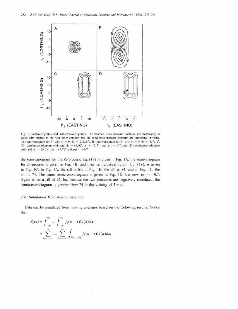
Fig. 1. Semivariograms and semicrossvariograms. The hatched lines indicate contours are decreasing invalue with respect to the next inner contour, and the solid lines indicate contours are increasing in value.(A) semivariogram for ZI with VI = 0, (Jl = (2,2,2)', (B) sen1ivariogram for Z2 with V2 = 0, (J2 = (3,7,1 )',(C) semicrossvariogram with and Al = (0,0)', A2 = (5,7)' and PI2 = 0.7, and (D) semicrossvariogramwith and Al = (0,0)', A2 = (5,7)' and PI2 = -0.7
the semivariogram for the Zl-process, Eq. (18) is given in Fig. lA, the semivariogramfor Z2-process is given in Fig. IB, and their semicrossvariogram, Eq. (19), is givenin Fig. 1C. In Fig. 1A, the sill is 64, in Fig. 1B, the sill is 84, and in Fig. 1C, thesill is 74. The same semicrossvariogram is given in Fig. ID, but now Pl2 == -0.7.Again it has a sill of 74, but because the two processes are negatively correlated, thesemicrossvariogram is greater than 74 in the vicinity of h == A.
2.4. Simulation from moving averages
Data can be simulated from moving averages based on the following results. Noticethat
Zk(S) =I:· ..I: h(x - S)Yk(x)dx
= f ... f 1. . fk(X - s)Yk(x)dx,il =-CX) id=-CX) A(ll ,...,ld)

J.M. Ver Hoef, R.P. Barry/Journal of Statistical Planning and Inference 69 (1998) 275-294 283
where A(il , ... , id) is the small area (iI/aI, (i l + 1)/al) x ... x (id/ad, (id + 1)/ad) and
IA(il,,,.,id)1 == (l/al)(lja2)".(1/ad) for all {il,,,.,id}, so call it IAI. Now, if aj;j ==1, ... ,d, are quite large, then A(i l , ... , id) will be a small area and fk(X) will be
relatively constant over A(il, " ., id), so
with the approximation improving as all aj -----+ CX) for j == 1, 2, " . ,d because fk (x) is
Reimann integrable. But,
from the central limit theorem and the definition of white nOIse. Basically, we can
approximate white noise with a set of densely packed independent random numberswith small variance. Hence, we have
where Yk(i 1,,,., id) ~N(O, IA I).In practice, we use L~:=bj for LZ:-CXJ for some bj and Cj whenever Ifk(xj - sj)1
becomes relatively small or °below bj and above Cj' In order to get crosscorrelation
and shift, we simulate an (L+ 1)-variate vector [wo(x), WI (x), ... ,WL(X)J' of independentrandom variables Wk(X) rv N(O, IAI) at each location on the densely packed grid, and
create shifted correlation among the L-variates at each location by taking Yk(X) ==
VI - piWk(X) + Pkwo(x - Lf k). Finally, each variable can be given an additive whitenoise component and nonzero mean,
where Uk(S) is a simulated standard normal random variable. Notice that in order to
accommodate shifts and the moving average function, the original grid of densely
packed points may need to be substantially larger than f!fi.
2.5. Estimation of 2Ykm(h)
The method of moments estimator for the variogram is
(20)

(21 )
(22)
284 1. M. Ver Hoe}: R.P. Barry / Journal of Statistical Planning and Inference 69 (1998) 275-294
where h == Sj - Si, N(h) == {(Si, Sj) : Sj - Si == h} and IN(h)1 is the number of distinctelements in N(h). The en1pirical variogram, Eq. (20), is unbiased for Eq. (1). Recall
Rk(s) == Zk(S) - f.1k, so let rk(s) =- Zk(S) - Zk, where Zk is the mean of the kth variable.Then the n1ethod of moments estimator of the covariogram is,
" 1 '""Ckk(h) = IN(h)1 L/k(sdrk(Sj),N(h)
which is biased for Eq. (6). The estimator given by Eq. (21) is biased because it is
necessary to estimate the mean f.1k of the spatial process with the mean of the realization
Zk (Cressie 1991, p. 70). It is the lack of bias that makes variogram estimation 'better'than covariogram estimation.
It is also necessary to estimate the crossvariogram for the zero-mean residual process
Rk(-). Then a method of moments estimator of 2}'km(h) for the Rk(-) is,
"h 1 '"""" 22Y/an( ) = IN(h )1 L..)rk(Si) - rm(Sj)JN(h)
where again h == Sj - Si. Papritz et al. (1993) also suggest this estimator, and note thatit is biased. Another problem that we encountered with Eq. (22) is that estimation is
poor when the variance of Rk (.) is orders of magnitude different from that of Rm( - ),
and (Cressie 1991, p. 141) suggests standardizing the data by (Zk(S)-f.1k)/Vvar(zk(s)).
We propose a two-step method for estimating crossvariogram parameters. As discussed in the previous section, estimation for the variogram parameters () and v is
generally good (unbiased), and is likely better than trying to re-estimate them in the
crossvariogram (biased). Thus, we might as well use the parameters () and v as esti
mated for the variogram and plug them into the formula for the crossvariogram. That
leaves only the parameters Pk, Pm, Ak , and Am to estimate in the crossvariogram. Onepossibility is to minimize a weighted least squares,
WLSkm == L IN(h)l[empirical- model]2.all h
(23 )
For the variogram, empirical is 2Ykk(h) from Eq. (20) and model is 2Ykk(hl()k, Vk) fromEq. (10), and then Eq. (23) is minimized for ()k and Vk. For the crossvariogram, en1pir
ical is 2Ykm(h) from Eq. (22) and model is 2Ykm(hl(), v,Pk,Pm,Ak,A m) from Eq. (11),
and then Eq. (23) is minimized for Pk, Pm, Ak , and Am, taking () and v as estimated fromthe variogram. Recall that there is some nonidentifiability in Pk (for L == 2) and Ak,. As
suggested earlier, one sin1ply identifies P as PI P2 and one could choose Al == 0, and
shifts in Z2 are relative to ZI. For L? 3, the remaining parameters Ak , k == 2, ... ,L, are
identifiable, as are Pk, k == 1, ... ,L . For L? 3, the two-step procedure is: (1) estimate
() and v for each variogram separately using WLSII, ... ,WLSLL , and then, (2) use theredundancy in the crossvariograms to minimize WLS 12 +...+WLSL ,L-I simultaneously
1. M. Ver Hoef, R.P. Barry / Journal of Statistical Planning and Inference 69 (1998) 275-294 285
for the p'sand j's. Another possibility is to minimize all parameters simultaneously
for all WLS ll + ... + aLLWLSLL + al2WLS l2 + ... + aL, L-I WLSL,L-I, where weights
akm can adjust for different sample sizes, etc. This may be computationally difficult if
L is large.
In the absence of more research, use of Eq. (22) in Eq. (23) for crossvariogram
fitting is both intuitive and sin1ple. There are other possibilities, however. For example,
Cressie (1985) shows that, for kriging, minimizing,
L IN(h)1 ( 2Ykk(h) _ 1)2,2Ykk(hIOk,Vk)
all h
is better than Eq. (23), as it puts more weight on a closer fit near the origin, which is the
most critical area for kriging (Stein, 1988). However, accurate estimation of the sill for
each 2Ykk(h) is also needed in order to estimate the Pk'S properly in the crossvariogram,
which is important because Pkm controls how much 'information' cokriging uses from
each covariate. Hence, it is not clear that we should use increased weighting near the
origin for variogram and crossvariogram estimation.
3. Cokriging and multivariable spatial prediction
After estimating all parameters, the full crossvariogram is defined and can be used for
cokriging and multivariable spatial prediction as follows. Suppose we want to predict
the full vector Z (so), and call the predictor p(So Iz), where the data Z =: (z~ , z~, ... , ZL)'
and Zk =: [Zk(Slk ),Zk(S2k), ... ,zk(snk)J' with nk not necessarily equal to nm . Then the
prediction weights
lOll £012 £OIL
£021 £022 W2LQ=:
lOLl WL2 lOLL
are a solution to
(~:) (~) (~) , (24 )
where
TIl T I2 TIL
T21 T 22 T 2LT=:
T LI T L2 T LL
286 J.M. Ver Hoef, R.P. Barry/Journal of Statistical Planning and Inference 69 (1998) 275-294
and r km has as its (i,j)th element 'Ykm(Si, Sj \0, V, Pk' Pm' 1k,1m) and r kk has as its (i,j)th
element 'Ykk(Si, Sj 10k, \\); and where
G=
1'L1 1'L2 1'LL
and 1'km has as its ith element 'Ykm(Si, So 10, V, Pk' Pm' 1k,1m), and 1'kk has as its ith element
'Ykk(Si, So 10k, Vk); and where
l(nl Xl) 0 0 1 0 0
0 1(n2 X 1) 0 0 1 0x= 1=
0 0 l(nL x 1) 0 0 (LxL)
and A is a diagonal matrix of Lagrange multipliers. Eq. (24) yields the multivariable
predictor
(25)
with MSPE matrix,
where
D=
"Ill (So, so) 'Y12(SO, so)
'Y21(SO,SO) 'Y22(SO,SO)
'Y1L(SO, so)
'Y2L(SO, so)
Details of results given in Eqs. (24 )-(26) are given in Ver Hoef and Cressie (1993).
Each element of peso Iz) is the cokriging predictor. The cokriging mean-squared-predic
tion errors are the diagonal elements of Eq. (26), and crossvariable prediction covariation is given by the off-diagonal elements of Eg. (26).
4. Examples
We will illustrate these methods with simulated data because all of the properties
(i.e., the true parameter values) of the data are known. The simulations are in one
dimension, using the moving average functions, Egs. (12) and (13), given earlier. These
examples illustrate simulating data using moving averages, estimating the variogram andcrossvariogram, fitting models to the empirical variograms and crossvariograms, and
J.M. Ver Hoef, R.P. Barry / Journal of Statistical Planning and Inference 69 (1998) 275-294 287
then using the fitted variogram and crossvariograms for cokriging and multivariablespatial prediction.
Independent pairs of correlated data, Yl (Xi) and Y2(Xi) were sin1ulated from a bivariate standard normal distribution with some P (because we have only 2 variables,
here we suppress the subscript on Plan), Xi == 0.25,0.50,0.75, ... ,400, so i == 1, ... , 1600such pairs were independently generated. Two other sets of data, U1 (s) and U2(S),
s == 101, 102, ... ,400 were also simulated independently, each from a standard normaldistribution. Then the Zl -process was constructed from,
1600
Zl(S) == L VO.25Yl(Xi)!1(Xi - sI8 11 ,812 ) + V1 U1(S) + /11,
i=l
for S == 101, 102, ... ,400; also notice that J 1 == O. The Z2 -process was constructed from
1600
Z2(S) == L VO.25Y2(Xi - J)!2(Xi - s1821 , ( 22 ) + V2 U2(S) + /12,
i=l
for S == 101, 102, ... ,400, where 82, j ~ O. Notice that because J 1 == 0 we suppress useof subscripts for J 2. The {S == 1, ... , 100} were not used to allow for the shift incorrelation structure and to minimize edge effects. The data sets were then re-indexedon the integers fron1 1,2, ... ,300.
Two examples are given. The second example has a nugget effect, while the firstdoes not, and the first example illustrates cokriging (prediction of a single component)while the second example illustrates multivariable spatial prediction (bivariable, in thiscase ).
4.1. Example 1: empirical estimation and fitting models
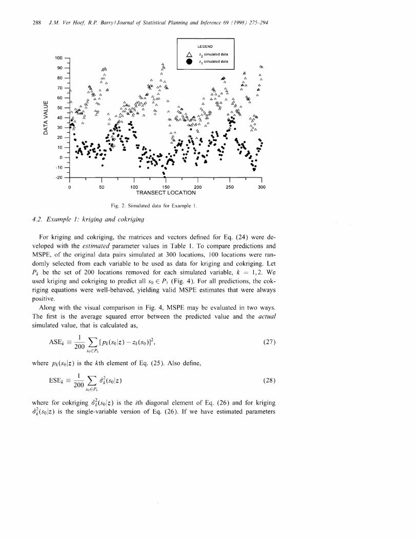
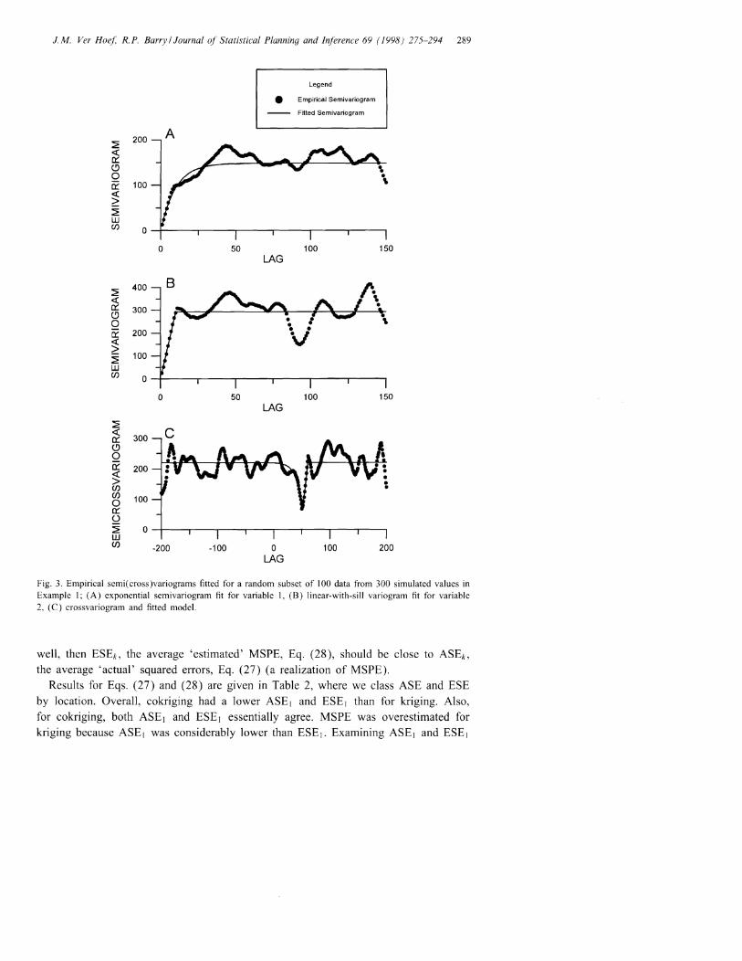
Data were simulated with P == 0.9 and J == 50, with 811 == 5, 812 == 0.1, VI == 0 and/11 == 10 for Zl (.), and with 821 == 5, 822 == 10, V2 == 0, and /12 == 50 for Z2(.) (Fig. 2).Notice that no nugget effect was added to these simulations. The empirical variogramswere calculated for Zl (.) and Z2(.) using Eq. (20), and are given in Fig. 3A andFig. 3B, respectively. The empirical crossvariogran1 was calculated using Eq. (22), andis given in Fig. 3C. The model given by Eq. (14) was fit to the empirical variogramof Zl ( .); and the model given by Eq. (15) was fit to the empirical variogram of Z2 ( • ),
using Eq. (23) for both minimizations. The crossvariogran1 n10del, Eq. (16), was fitto the empirical crossvariogram using the variogram estimates 0 of f) and minimizingEq. (23) for P and J. All minimization used the downhill simplex method of NeIderand Mead (1965). Table 1 gives the true values and the estimated values for allparameters. The fitted variograms and crossvariograms are also shown in Fig. 3. Thissimulated example demonstrates that estimation of the variogram and crossvariogramparameters also estimates the moving average parameters. The shift parameter J causesthe semicrossvariogram to be asymmetric in h and not centered on 0 (Fig. 3C). Webelieve this is the first time such a model has been presented.
288 J. M. Ver Hoef, R.P. Barry / Journal of Statistical Planning and Inference 69 (1998) 275-294
LEGEND
Z2 simulated data
z1 simulated data100
90
80
70
60W::> 50....J~
> 40«I- 30~0
20
10
0
-10
-20
0 50 100 150 200TRANSECT LOCATION
Fig. 2. Simulated data for Example 1.
250 300
4.2. Example 1: kriging and cokriging
For kriging and cokriging, the matrices and vectors defined for Eq. (24) were de
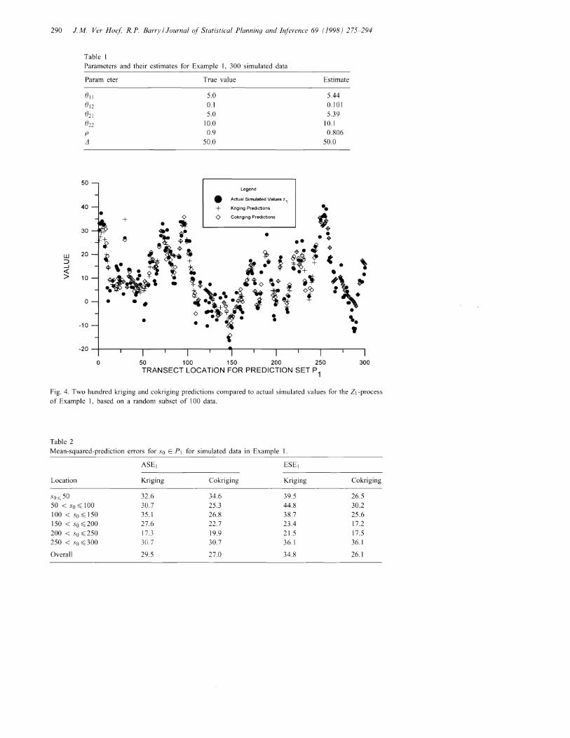
veloped with the estimated parameter values in Table 1. To compare predictions andMSPE, of the original data pairs simulated at 300 locations, 100 locations were ran
don1ly selected from each variable to be used as data for kriging and cokriging. LetPk be the set of 200 locations removed for each simulated variable, k = 1,2. We
used kriging and cokriging to predict all So E PI (Fig. 4). For all predictions, the cokriging equations were well-behaved, yielding valid MSPE estimates that were alwayspositive.
Along with the visual comparison in Fig. 4, MSPE may be evaluated in two ways.The first is the average squared error between the predicted value and the actualsimulated value, that is calculated as,
(27)
where Pk(solz) is the kth element of Eq. (25). Also define,
(28)
where for cokriging a~(solz) is the ith diagonal element of Eq. (26) and for kriginga~(solz) is the single-variable version of Eq. (26). If we have estimated parameters
J.M. Ver Hoef; R.P. Barry/ Journal of Statistical Planning and Inference 69 (1998) 275-294 289
Legend
• Empirical Semivariogram
Fitted Semivariogram
200 A:E~0::C>0~ 100~
~:Ewen 0
0 50 100 150LAG
400 B~~~ 300(90(i: 200
~ 100~WCJ)
0
0 50 100 150LAG
~«300~
(900:: 200 •~
••CJ)CJ) 1000~
0~ aw(f) -200 -100 0 100 200
LAG
Fig. 3. Empirical semi(cross )variograms fitted for a random subset of 100 data from 300 simulated values inExample 1; (A) exponential semivariogram fit for variable 1, (B) linear-with-sill variogram fit for variable2, (C) crossvariogram and fitted model.
well, then ESEk , the average 'estimated' MSPE, Eq. (28), should be close to ASEk ,
the average 'actual' squared errors, Eq. (27) (a realization of MSPE).Results for Eqs. (27) and (28) are given in Table 2, where we class ASE and ESE
by location. Overall, cokriging had a lower ASE 1 and ESE 1 than for kriging. Also,for cokriging, both ASE l and ESE} essentially agree. MSPE was overestimated forkriging because ASE l was considerably lower than ESE l . Examining ASE l and ESE]
290 1. M. Ver Hoe;; R.P. Barry / Journal of Statistical Planning and Inference 69 (1998) 275-294
Table 1Parameters and their estimates for Example 1, 300 simulated data
Param eter
50
True value
5.0
0.1
5.010.00.9
50.0
Estimate
5.44
0.101
5.3910.10.806
50.0
w:::>....J
~
40•
30
20
10
o
-10
•
+
• ••
e+o
Legend
Actual Simulated Values z1
Kriging Predictions
Cokriging Predictions
•
o 50 100 150 200 250TRANSECT LOCATION FOR PREDICTION SET P1
300
Fig. 4. Two hundred kriging and cokriging predictions compared to actual simulated values for the 2} -process
of Example 1, based on a random subset of 100 data.
Table 2Mean-squared-prediction errors for So E PI for simulated data in Example 1.
ASE} ESE}
Location Kriging Cokriging Kriging Cokriging
so~ 50 32.6 34.6 39.5 26.5
50 < so:( 100 30.7 25.3 44.8 30.2
100 < so:( 150 35.1 26.8 38.7 25.6
150 < so:( 200 27.6 22.7 23.4 17.2
200 < so:( 250 17.3 19.9 21.5 17.5250 < so:( 300 30.7 30.7 36.1 36.1
Overall 29.5 27.0 34.8 26.1
1. M. Ver Hoe/: R. P. Barry / Journal of Statistical Planning and Inference 69 (1998) 275-294 291
Table 3Mean-squared-prediction errors for So E P2 for simulated data in Example 1.
ASE2 ESE}
Location Kriging Cokriging Kriging Cokriging
so~ 50 40.0 40.1 55.1 55.0
50 < So ~ 100 55.4 56.5 62.6 48.7
100 < So ~ 150 32.3 28.8 48.7 42.6
150 < So ~200 40.5 39.9 51.8 41.6
200 < So ~250 37.6 33.3 40.8 30.5
250 < So ~300 91.0 32.4 60.0 36.7
Overall 49.2 38.4 53.2 42.7
by location class for both kriging and cokriging, notice that both methods did more
poorly at the ends, as opposed to the middle, as expected (Table 2). An interesting
feature of Table 2 is that, for So > 250, cokriging became essentially the same as
kriging, and this may be seen in Fig. 4 as well. This makes sense, because all of
the 'information' in the Z2-process, for predicting the ZI-process, was shifted forward
Ll = 50. Hence, there is no reason to use data Z2(Si) when predicting so> 250 for the
ZI -process. In fact, we might expect that because of the shift Ll, cokriging would do
quite a bit better than kriging for smaller So, but that this advantage would taper off
as So increases; in general, Table 2 does show this pattern.
The same analysis was carried out for prediction of the set P2 for the Z2 -process. We
used kriging and cokriging to predict all So E P2 . The MSPE results, in Table 3, show
that cokriging was a dramatic improvement over kriging because ASE2 for cokriging
is much lower than ASE2 for kriging. Both kriging and cokriging slightly overesti
mated MSPE because ASE2< ESE2 for both. Also notice that in Table 3, kriging and
cokriging are essentially the sanle for So ~ 50, as expected.
4.3. Exanzple 2: en1pirical estbnation and ,tittin?] lnodels
For the second example, data were simulated with p = 0.8 and L1 = 50, and with
011 =2,0 12 =0.1, VI =4, and III = 10 for ZI(-), and with (]21 = 1, (}22 = 15, V2 =3, and
Il2 = 20 for Z2 (-). Of these, 100 locations were randomly selected and both data values
were retained. In this example, we added a nugget effect and estimated parameters for
all 300 data and the random subset of 100. As in the first exanlple, we use Eqs. (20)and (22) for empirical estimation of semivariograms and the semicrossvariogram, and
fit models of Eqs. (14) and (16) to the empirical estimates by minimizing Eq. (23).The parameter estimates are given in Table 4.
4.4. Exalnple 2: lnultivariahle spatial prediction
Using only bivariate data at the 100 data points and the paranleter estinlates based
on these 100 data, the 200 bivariate data that were set aside were predicted. For each
292 J.M. Ver Hoef, R.P. Barry / Journal of Statistical Planning and Inference 69 (1998) 275-294
Table 4Parameters and their estimates for simulated data in Exan1ple 2.
Parameter True value est n = 300
811 2.0 2.16812 0.1 0.129
VI 4.0 4.03821 1.0 0.962
822 15.0 12.5
V2 3.0 2.91p 0.8 0.817L1 50.0 48.7
est n = 100
2.03 phantomO0.1224.091.06
13.32.580.834
48.7
Note: Estimation was for all 300 simulated data (colun1n 3) and a random subset (column 4).
prediction, we obtained the MSPE matrix, Eq. (26). For each location, assuming prediction errors are normally distributed, bivariate prediction regions may be developed,as shown by Ver Hoef and Cressie (1993). The average of each element in the n1atrix,Eq. (26), over the 200 prediction sites, was
(23.5
- 0.0298- 0.0298)
10.6 '(29)
showing a very slight negative correlation between the two predicted values. Note thatESE 1 and ESE2 are the first and second diagonal elements of Eq. (29). For the firstvariable ASE 1 was 23.9 and for the second variable ASE2 was 12.3, indicating reasonable closeness between estimated and actual squared-prediction errors, even though allestimation and prediction was based only on the random subset of 100. By comparison,kriging only variable 1 gave ESE 1 == 24.8 and ASE 1 == 26.2, and kriging only variable2 gave ESE2 == 11.0 and ASE2 == 12.0. Because of the rather large nugget effect thetwo variables are essentially independent, so the advantage of cokriging over krigingis not as apparent as in Example 1.
5. Discussion and conclusions
The use of integration of a moving average function over white noise random processes, Eq. (8) leads to construction of valid variograms and crossvariograms. Theresulting crossvariogram, Eq. (11), can allow for modeling crossvariograms for a widevariety of component variograms. The examples illustrate the development and fittingof models, and then using them for spatial prediction. The first simulation exampleillustrates fitting models to data, and demonstrates that cokriging can have a considerable advantage over kriging. The second simulation example illustrates multivariablespatial prediction, also showing that estimation on a subset of 100 locations is still quitegood, and that the nugget effect diminishes the advantages of cokriging over kriging.Both of these examples contain a nonzero shift parameter L1 that causes asymmetry in
J.M. Ver Hoef, R.P. Barry/ Journal of Statistical Planning and Inference 69 (1998) 275-294 293
the covariogram, i.e., Ckm(h) # Ckm ( -h), so the use of the traditional crossvariogram,Eq. (5), would not be optinlal. Real-world processes that might be expected to containsuch a shift would be things like weather temperatures, where Z1 (.) are temperatureson one day and Z2(.) are temperatures on the following day. Air mass movementwould cause crosscorrelation to be shifted.
With the methods outlined in this paper, use of the crossvariogram, Eq. (7), in placeof the traditional crossvariogram, Eq. (5), eliminates all three of the main problemslisted in the introduction: (1) the symnletrical covariance assumption, Ckm(h )== Ckm (-h),(2) data on each variable do not need to come from the same location in order to estimate the crossvariogram, and, (3) we can consider models beyond those of coregionalization. Coregionalization assumes that the crossvariogram has a functional form likea variogram; i.e., it is linear, exponential, spherical, etc. Figs. 1 and 3 show why coregionalization is inflexible and has performed poorly in the past. Crossvariogram modelshave functional forms that may be considerably different than those of variograms!
So far, we have only considered variogram models with sills. Now consider themoving average function,
where J~cxJ.fk(xIOk)]2 d.x == 00. Still, we can use Eq. (10), which implies a linearvariogram. However, now the integral in Eq. (11) will be finite only if !k(X) and.f~l(X) have the same height (fh == 8m ). In general, we see that asymptotically as x ----+ 00
there can not be too nluch area in [!k(X)- !m(X )]2. This leads us to the sanle conclusionas Papritz et al. (1993), that a linear variogram for Z1 (.) implies that the variogramfor Z2 (.) must have the same slope for the crossvariogranl to exist. It should notbe too surprising that variogranl models without sills cause potential difficulties whencokriging, considering that they have unbounded variation; i.e., the linear variogramdescribes Brownian nlotion.
More research is needed on estimation and fitting methods for the crossvariogranlused in cokriging and multivariable spatial prediction. For exanlple, unlike variogramversus covariogram estimation, for crossvariograms it is necessary to subtract the meanfrom each variable, and possibly rescale them, so there may be no advantage to es
timating crossvariograms as opposed to estimating crosscovariances. In addition, wepropose a weighted least squares criterion to fit variograms first, and fit any additionalcrossvariogram paranleters as a second step, but simultaneous fitting of all parametersis also attractive.
Acknowledgenlents
Support for this work was provided by Federal Aid in Wildlife Restoration to theAlaska Department of Fish and Game and the Eli-Lander Foundation. We thank NoelCressie, Andy Royle, and one anonymous reviewer for their comments.
294 1. M. Ver Ho~t: R. P. Barry / Journal of Statistical Planning and Inference 69 (1998) 275-294
References
Barry, R.P., Ver Boef, J.M., 1996. Blackbox kriging: spatial prediction without specifying variogram models.
J. Agricul. Biological Environment. Statist. 1, 297-322.Clark, L Basinger, K.L .. Harper, W.V., 1989. MUCK -- A novel approach to cokriging. In: Buxton,
B.E. (Ed.), Proc. Conf. Geostatistical, Sensitivity, and Uncertainty Methods for Ground-Water Flow andRadionuc1ide Transport Modeling, Batelle Press, Columbus, pp. 473-479.
Cressie, N., 1985. Fitting variogram models by weighted least squares. J. Internat. Assoc. Math. Geology17,693--702.
Cressie, N., 1991. Statistics for Spatial Data. Wiley, New York.
Helterbrand, J.D., Cressie, N., 1994. Universal cokriging under intrinsic coregionalization. Math. Geol. 26,205-226.
Isaaks, E.H., Srivastava, R M., 1989. An Introduction to Applied Geostatistics. Oxford University Press, NewYork.
JourneL A.G., Huijbregts, C.1., 1978. Mining Geostatistics. Academic Press, London.Lu, H., Zimmennan, D.L., 1994. A nonparametric approach to testing for directional sYlnmetry of spatial
correlation. Technical Report 234, Depa11ment of Statistics and Actuarial Science, University of Iowa,Iowa City, Iowa.
Ivlyers, D.E., 1982. Matrix formulation of cokriging. Math. Geol. 14, 249-257.Myers, D. E., 1991. Pseudo crossvariograms, positive-definiteness, and cokriging. Math. Geol. 23, 805--816.Nash, M.S., Toonnan, A., Wierenga, PJ., Gutjahr, A., Cunninghaln, G.L., 1992. Estinlation of vegetative
cover in an arid rangeland based on soil-moisture llsing cokriging. Soil Sci. 154, 25-~36.
NeIder, .J.A., Mead, R., 1965. A simplex method for function minimization. Comput. J. 7,308-313.Papritz, A., Kunsch, H.R., Webster, R., 1993. On the pseudo cross-variogram. Math. Geo!. 25, 1015-1026.Stein, M.L., 1988. Asymptotically efficient prediction of a random field with a misspecified covariance
function. Ann. Statist. 16, 55--63.Ver Hoef, J.M .. Cressie, N., 1993. Multivariable spatial prediction. Math. Geol. 25, 219-240. [Erratum, 1994.
Math. Geol. 26, 273-275.]Wackemagel, H., 1995. Multivariate Geostatistics. Springer, Berlin.Yaglom, A.M., 1987. Correlation Theory of Stationary and Related Random Functions I: Basic Results.
Springer, New York.