construct validation in organizational behavior...
TRANSCRIPT

Construct Validation 1
Construct Validation in Organizational Behavior Research
Jeffrey R. Edwards
University of North Carolina
The author thanks Richard P. DeShon, Fritz Drasgow, and Larry J. Williams for their helpful
comments on an earlier version of this chapter.
In J. Greenberg (Ed.), Organizational behavior: The state of the science (2nd ed., pp. 327-371).
Mahwah, NJ: Erlbaum, 2003.

Construct Validation 2
A theory comprises two sets of relationships, one that links constructs that constitute the
substance of the theory, and another that maps constructs onto phenomena that can be directly
observed and measured (Bagozzi & Phillips, 1982; Costner, 1969). In organizational behavior
(OB) research, theory development emphasizes relationships among constructs but devotes
relatively little attention to relationships between constructs and measures (Schwab, 1980).
These latter relationships are crucial to theory development, because they provide the means by
which constructs become accessible to empirical research and theories are rendered testable.
Moreover, because the relationships between constructs and measures are integral to a theory,
theory testing is incomplete unless these relationships are scrutinized. Thus, the relationships
between constructs and measures constitute an auxiliary theory that itself is subject to empirical
testing and falsification (Costner, 1969; Cronbach & Meehl, 1955; Schwab, 1980).
Relationships between constructs and measures are the essence of construct validity. At
its most fundamental level, construct validity concerns the degree to which a measure captures
its intended theoretical construct (Cronbach & Meehl, 1955). Although the notion of construct
validity is straightforward, procedures used to assess construct validity are complex and have
evolved considerably during the past several decades. These procedures present a potentially
bewildering array of choices for OB researchers confronted with crucial task of establishing the
correspondence between theoretical constructs and their measures.
This chapter provides a chronological treatment of approaches to construct validation.
The chapter begins by defining constructs and measures, the basic elements of construct
validation. Construct validity is then defined and distinguished from other forms of validity.
Next, approaches to construct validation are discussed, focusing on formulations of the
relationship between constructs and measures and statistical procedures to assess reliability and
Construct Validation 3
convergent and discriminant validity. These approaches are organized chronologically in terms
of classical approaches prevalent from the 1950s through the 1970s, modern approaches of the
1980s and 1990s, and emerging approaches that capture recent developments and future trends.
The chapter concludes with recommendations for assessing and enhancing the construct validity
of measures used in OB research.
Definitions
This section offers definitions of the terms construct, measure, and construct validity.
Definitions of these terms have evolved over the years, as evidenced by successive publications
of the American Psychological Association standards for educational and psychological testing
(American Psychological Association, 1966, 1985, 1999) and treatises on construct validity by
Campbell (1960, 1996), Cronbach (1971, 1989; Cronbach & Meehl, 1955), and Messick (1975,
1981, 1995). However, the nuances that mark this evolution are anchored in core ideas that have
remained stable. This stability is reflected in the definitions adopted here, which provide a
consistent backdrop against which to track the development of construct validation procedures.
Construct
A construct is a conceptual term used to describe a phenomenon of theoretical interest
(Cronbach & Meehl, 1955; Edwards & Bagozzi, 2000; Messick, 1981). Constructs are terms
researchers invent to describe, organize, and assign meaning to phenomena relevant to a domain
of research (Cronbach & Meehl, 1955; Messick, 1981; Nunnally, 1978; Schwab, 1980).
Although constructs are literally constructed, or put together, by researchers (Nunnally, 1978;
Schwab, 1980), the phenomena constructs describe are real and exist independently of the
researcher (Arvey, 1992; Cook & Campbell, 1979; Loevinger, 1957; MacCorquodale & Meehl,
1948; Messick, 1981). For example, attitudes such as job satisfaction and organizational

Construct Validation 4
commitment are real subjective experiences of people in organizations, and characteristics of
social relationships such as trust and conflict are real to people engaged in those relationships.
Although constructs refer to real phenomena, these phenomena cannot be observed directly or
objectively. Rather, researchers view these phenomena through the distorted epistemological
lenses that constructs provide and rely on flawed measures that yield imperfect empirical traces
(Cook & Campbell, 1979; Loevinger, 1957; Messick, 1981). This definition represents a critical
realist perspective on the meaning of constructs (Bhaskar, 1978; Cook & Campbell, 1979). It is
realist because it asserts that constructs refer to actual psychological and social phenomena that
exist separately from our attempts to study them, and it is critical because it recognizes that these
phenomena cannot be assessed with complete accuracy, due to imperfections in our sensory and
methodological apparatus (Cook & Campbell, 1979; Delanty, 1997; Loevinger, 1957; Messick,
1981; Zuriff, 1998).
Measure
A measure is an observed score gathered through self-report, interview, observation, or
some other means (DeVellis, 1991; Edwards & Bagozzi, 2000; Lord & Novick, 1968; Messick,
1995). Put simply, a measure is a quantified record, such as an item response, that serves as an
empirical representation of a construct. A measure does not define a construct, as in strict
operationalism (Campbell, 1960; Cronbach & Meehl, 1955), but rather is one of various possible
indicators of the construct, all of which are considered fallible (Messick, 1995). As defined here,
a measure is not an instrument used to gather data, such as a questionnaire, interview script, or
observation protocol, nor is it the process by which data are generated and gathered (Alreck &
Settle, 1995; Rea & Parker, 1992; Sudman, Bradburn, & Schwarz, 1996). Rather, a measure is an
observed record or trace that serves as imperfect empirical evidence of a construct.
Construct Validation 5
Construct Validity
Construct validity refers to the correspondence between a construct and a measure taken
as evidence of the construct (Cronbach & Meehl, 1955; Nunnally, 1978; Schwab, 1980).
Construct validity does not refer to the inherent properties of a measure or instrument. Instead, it
concerns the degree to which a measure represents a particular construct and allows credible
inferences regarding the nature of the construct (Cronbach, 1971; Cronbach & Meehl, 1955).
Thus, a particular measure may demonstrate different degrees of construct validity depending on
the construct for which the measure is taken as evidence. Moreover, construct validity is not an
all-or-nothing phenomenon, such that a measure that demonstrates certain properties is deemed
construct valid. Rather, construct validity is a matter of degree based on the cumulative evidence
bearing on the correspondence between a construct and measure (Cronbach & Meehl, 1955).
Finally, construct validation is not a task that is accomplished and then set aside. To the contrary,
construct validation is an ongoing process, such that each application of an instrument provides
further evidence regarding the construct validity of the instrument and the measures it generates
(Cronbach, 1989; Nunnally, 1978).
Construct validity may be separated into trait validity and nomological validity
(Campbell, 1960). Trait validity focuses on the relationship between the construct and measure
isolated from the broader theory in which the construct is embedded. Evidence for trait validity is
provided by convergence of measures intended to represent the same construct and divergence
among measures designed to represent different constructs. Convergence of measures sharing the
same method (e.g., all self-report) indicates reliability, whereas convergence of measures using
different methods represents convergent validity (Campbell, 1960; Campbell & Fiske, 1959).
Divergence among measures using the same or different methods demonstrates discriminant
Construct Validation 6
validity (Campbell, 1960; Campbell & Fiske, 1959). Reliability and convergent validity provide
evidence for a construct acting as a common cause of the measures, and discriminant validity
provides evidence against the intrusion of other unintended constructs (Messick, 1995).
Nomological validity is based on evidence that measures of a construct exhibit relationships with
measures of other constructs in accordance with relevant theory (Carmines & Zeller, 1979;
Cronbach & Meehl, 1955). Thus, nomological validity entails the evaluation of a measure within
a broader theory that describes the causes, effects, and correlates of the construct and how they
relate to one another (Campbell, 1960; Cronbach & Meehl, 1955).
Construct validity may be distinguished from content validity and criterion-oriented
validity (Nunnally, 1978). Content validity is the degree to which a measure represents a
particular domain of content. Content validity is achieved by defining the content domain of
interest, selecting or developing items that represent the domain, and assembling the items into a
test, survey, or other instrument. Content validity is not assessed using empirical or statistical
procedures, but instead relies on “appeals to reason” (Nunnally, 1978, p. 93) that the procedures
used to develop an instrument ensure that important content has been adequately sampled and
represented.1 Criterion-oriented validity refers to the relationship between the measure of
interest and some criterion measure deemed important, such as job performance. Criterion-
oriented validity places less emphasis on the conceptual interpretation of a measure than on its
ability to predict a criterion.
Construct validity may be distinguished from other forms of validity that are vital to the
research process. Cook and Campbell (1979) organize these forms of validity into three broad
categories. Statistical conclusion validity is whether a study can establish the presence and
magnitude of the relationship between two variables. Internal validity concerns whether the
Construct Validation 7
relationship between a presumed cause and effect is free from alternative explanations that
implicate other causes or methodological artifacts. Finally, external validity is whether the
findings from a study can be generalized to other samples, settings, and time frames. Because
these forms of validity do not bear directly on the relationships between constructs and measures,
they are not discussed further in this chapter (for thorough treatments, see Cook & Campbell,
1979; Cook, Campbell, & Peracchio, 1990).
Construct Validation Approaches
The past several decades have brought significant developments in procedures used to
assess construct validity. These developments are signified by increasingly sophisticated views
of the relationship between constructs and measures and advances in statistical procedures for
assessing reliability and convergent and discriminant validity. Methods for studying nomological
validity have advanced as well, but these advancements have tracked general developments in
analyzing relationships among constructs, as marked by the evolution from analysis of variance
to multiple regression, path analysis, and structural equation modeling (Cohen, 1968; Jöreskog,
1974; Werts & Linn, 1970; Williams & James, 1994). These developments implicate the whole
of applied statistics, and reviewing them is well beyond the scope of this chapter. Rather, the
following discussion tracks the evolution of three core elements of construct validation: (a) the
specification of the relationship between constructs and measures; (b) reliability; and (c)
convergent and discriminant validity. These three elements provide a focused treatment of
construct validation approaches and encompass many important analytical developments that
deal specifically with mapping constructs onto measures. Moreover, these aspects of construct
validation should be addressed prior to investigating nomological validity, because if a measure
does not display construct validity when examined in isolation, it is unwise to embed the
Construct Validation 8
measure within a broader theoretical framework. Thus, the elements of construct validation
examined in this chapter are natural precursors to the essential task of nomological validation
(Cronbach & Meehl, 1955).
For expository purposes, the construct validation approaches discussed here are separated
chronologically into classical, modern, and emerging approaches to construct validation. The
boundary between classical and modern approaches roughly coincides with the advent of
confirmatory factor analysis (CFA), and the boundary between modern and emerging approaches
is marked by developments that increase the complexity of the relationship between constructs
and measures and relax traditional assumptions that underlie analytical procedures used for
construct validation. As will become evident, the classification of construct validation
approaches into these three time frames reflects their usage in the OB literature more than their
development in the statistical literature. For instance, although CFA is the hallmark of modern
approaches to construct validation, its development predates its general use in the OB literature
by over a decade (Jöreskog, 1969). Likewise, some approaches that are just beginning to emerge
in the OB literature, such as generalizability theory (DeShon, 2002), can be traced back more
than three decades (Cronbach, Gleser, Nanda, & Rajaratnam, 1972). These time lags are natural
for the development and use of methodological procedures in general, and it is hoped that this
chapter will help accelerate the diffusion of recently developed construct validation procedures
in OB research.
Classical Approaches
Classical approaches to construct validation are rooted in seminal work on measurement
and psychometric theory of the 1950s and 1960s (e.g., Campbell, 1960; Campbell & Fiske, 1959;
Cronbach & Meehl, 1955; Lord & Novick, 1968; Nunnally, 1967). This work laid the foundation

Construct Validation 9
for conceptualizing and analyzing relationships between constructs and measures and established
the language of construct validation. These approaches are discussed below.
Relationship between constructs and measures. The fundamental equation of classical
measurement theory (Gulliksen, 1950; Lord & Novick, 1968) is as follows:
Xi = T + ei (1)
where Xi is the ith measure of T, T is an unobserved true score, and ei is measurement error,
which encompasses all sources of variance in Xi other than T. It is assumed that ei is a random
variable with zero mean and is uncorrelated with T and with the true scores and errors of other
measures (Lord & Novick, 1968). Figure 1 portrays the relationships between a single true score
and three measures, along with their associated error terms (in this and subsequent figures,
variables that signify constructs are represented by circles, and variables that represent measures
are indicated by squares). As will be seen, Figure 1 provides a useful point of departure for
comparing classical measurement theory to modern and emerging approaches to construct
validation.
---------------------------------
Insert Figure 1 about here
---------------------------------
The interpretation of Equation 1 in terms of the relationship between a construct and
measure hinges on the meaning of the true score T. In classical measurement theory (Lord &
Novick, 1968; Nunnally, 1978), a true score is typically defined as the hypothetical average of an
infinite number of scores for a particular subject. As the number of scores constituting the
average approaches infinity, the proportion of error variance in the average approaches zero.
Therefore, a true score may be interpreted as a subject’s score on Xi that is free from random

Construct Validation 10
measurement error. This score might not accurately represent the value of the construct, because
any systematic errors in Xi, such as mean bias or floor and ceiling effects, become part of the
hypothetical average that defines the true score (Cronbach et al., 1972). Thus, a true score may
be interpreted as the value of a construct for a subject if: (a) the measure Xi is unbiased, such that
repeated measures of Xi converge on the correct value of the construct; and (b) measurement
errors are uncorrelated with the construct, such that errors do not tend to be positive or negative
depending on the level of the construct (Lord & Novick, 1968). These assumptions are adopted
in the following discussion, thereby framing T as the value of the construct of interest.
Equation 1 allows several useful derivations that provide the basis for understanding the
correspondence between constructs and measures. We begin with the variance of Xi, which may
be written as:
V(Xi) = V(T + ei)
= V(T ) + V(ei) + 2C(T,ei)
= V(T ) + V(ei) (2)
where V(.) and C(.) refer to the variance and covariance, respectively, of a given term for
multiple subjects. Equation 2 follows from standard rules of covariance algebra and the
assumption that T and ei are uncorrelated. From Equation 2, it can be seen that the variance of a
measure is the sum of the variance of the true score and the variance of measurement error.
Because a true score signifies an error-free measure of a construct, V(T ) indicates the amount of
variance in X that is attributable to the construct. Naturally, it is desirable for V(T ) to be large
relative to V(ei).
Next, consider the covariance of Xi with T, which captures the magnitude of the
relationship between a measure and its associated construct:

Construct Validation 11
C(Xi,T) = C[(T + ei),T]
= C(T,T ) + C(T,ei)
= V(T ). (3)
Equation 3 indicates that the covariance between a measure and its true score, and hence the
construct of interest, is represented by the variance of the true score.
Finally, the covariance between two measures, designated here as Xi = Tp + ei and Xj = Tq
+ ej, may be written as:
C(Xi,Xj) = C[(Tp + ei),(Tq + ej)]
= C(Tp,Tq) + C(Tp,ej) + C(Tq,ei) + C(ei,ej)
= C(Tp,Tq). (4)
Equation 4 shows that the covariance between the true scores Tp and Tq equals the covariance
between their respective measures Xi and Xj. Thus, the covariance between the constructs
underlying two measures is indicated by the covariance between the measures themselves.
If Xi and Xj in Equation 4 refer to the same construct, they are termed congeneric,
meaning their true scores are perfectly correlated but need not have the same value. If Xi and Xj
have the same true scores, such that Tp = Tq = T, they are termed tau equivalent. Under tau
equivalence, C(Tp,Tq) = C(T,T ) = V(T ), which indicates that the covariances between all pairs of
tau equivalent measures have the same value and equal the variance of their common true score.
These properties also hold for measures that are essentially tau equivalent, which have true
scores that differ by no more than a constant (Novick & Lewis, 1967). Finally, if Xi and Xj have
the same true scores as well as the same error variances, such that V(ei) = V(ej) = V(e), they are
termed parallel. Because parallel measures have equal true score variances and equal error
variances, the measures themselves also have equal variances, which in turn implies that the

Construct Validation 12
covariances and correlations among pairs of parallel measures are equal. These principles and the
associated derivations form the basis of classical measurement theory and provide the foundation
for subsequent developments.
Reliability. Reliability refers to the proportion of true score variance in a measure. The
reliability of X may be expressed algebraically as follows:
ρXi = V(T )/V(Xi). (5)
For a single item, ρXi cannot be estimated, given that V(Xi) is known but V(T) is unknown. This
dilemma spawned various approaches to the estimation of reliability. One approach is based on
the notion of parallel measures of T. By definition, the correlation between parallel measures
equals their covariance divided by the product of their standard deviations. As noted previously,
the covariance between parallel measures equals V(T ), and the variances of parallel measures
have a common value V(Xi), which in turn implies that the product of their standard deviations is
also V(Xi). Hence, the correlation between parallel measures equals V(T )/V(Xi) and represents
the reliability of either measure. This reasoning underlies the alternative forms method of
reliability estimation (Carmines & Zeller, 1979; Nunnally, 1978). Although simple in concept,
this approach carries the practical problem of developing measures that meet the rather stringent
conditions of parallel measurement.
One way to address the problem of developing parallel measures is to administer the
same measure twice, based on the premise that a measure is parallel with itself. This approach
underlies the test-retest method of reliability estimation, which uses the correlation between a
measure collected on two occasions as an estimate of the reliability of the measure. The test-
retest approach has several drawbacks, such as the inability to distinguish low reliability from
actual change in the true score, practice and consistency effects that may inflate test-retest

Construct Validation 13
correlations, and the possibility that biases and other artifacts embedded in measurement errors
are correlated over time, thereby violating a key assumption of classical measurement theory
(Bohrnstedt, 1983; Nunnally, 1978).
An alternative to the test-retest approach is the split-half approach, in which a set of items
is administered on a single occasion and scores on the items are divided into two subsets. Given
that the subsets are drawn from the same set, they are considered alternative forms, which means
that their correlation represents the reliability of either subset. Because the subsets contain fewer
items than the full set, the correlation between the subsets of items underestimates the reliability
of a measure created by summing the full set. This underestimation can be corrected by applying
the Spearman-Brown prophecy formula (Nunnally, 1978):
21
21
r1r2
ρXX
XXX +
= (6)
where X1 and X2 are sums of items from the two split halves and 21 XXr is the correlation between
these sums. Despite its advantages, the split-half approach carries a fundamental ambiguity, in
that a set of items can be split in numerous ways, each of which may yield a different reliability
estimate.
The ambiguity of the split-half approach is resolved by Cronbach’s alpha (Cronbach,
1951), which equals the average of all possible split-half reliability estimates for a set of items.
Alpha may be interpreted as the proportion of true score variance in a sum of essentially tau
equivalent items. The intuition behind alpha can be grasped by considering the following sum of
k tau equivalent items:
)(11
i
k
ii
k
ieTX +∑=∑
==. (7)
The true score T is not indexed because it is assumed to be the same for all Xi. The variance of

Construct Validation 14
the item sum may be written as:
)](V[)V(11
i
k
ii
k
ieTX +∑=∑
==
)](...)()(V[ k21 eTeTeT ++++++=
)...(V k21 eeekT ++++=
)V()V(1
i
k
i
2 eTk=∑+= . (8)
The amount of true score variance in the sum is represented by k2V(T). Therefore, the proportion
of true score variance is k2V(T)/ )V(1
i
k
iX
=∑ . )V(
1i
k
iX
=∑ can be computed by taking the variance of
the item sum, and V(T) can be obtained by recalling that, for essentially tau equivalent items,
V(T) equals the covariance between any two items. Because all interitem covariances are equal
for essentially tau equivalent items, any one of the covariances will serve as an estimate of V(T).
In practice, interitem covariances usually vary, in which case it is sensible to use the average
interitem covariance to represent V(T) (McDonald, 1999). This approach leads to the following
equation for alpha (Cronbach, 1951):
)V(
),(Cα
1
2
i
k
i
ji
X
XXk
=Σ
= . (9)
An algebraically equivalent expression can be computed from the variances of the items and
their sum (Cronbach, 1951; Nunnally, 1978):
)V(
)V()V(
1α
1
11
i
k
i
i
k
ii
k
i
X
XX
kk
=
==
Σ
Σ−Σ
−= . (10)
The assumption of essential tau equivalence is crucial to alpha. To the extent this assumption is
violated, alpha underestimates the reliability of the item sum (Heise & Bohrnstedt, 1970). Hence,

Construct Validation 15
alpha should be considered a lower bound estimate of reliability and equals reliability when the
items constituting the sum are essentially tau equivalent.
Convergent and discriminant validity. Classical approaches to construct validation have
generally relied on two methods for assessing convergent and discriminant validity. One method
involves submitting measures to principal components analysis or common factor analysis and
determining whether measures of the same construct cluster together and measures of different
constructs separate from one another. The principal components model may be written as follows
(Harman, 1976; Kim & Mueller, 1978):
k1j XXXC jk2j2j1 b...bb +++=
i
k
iXji
1b
=∑= . (11)
where Cj represents the jth principal component and bji is a coefficient linking the ith measure to
the jth component. Equation 11 shows that a principal component is treated as a weighted linear
combination of measures, and measurement error is disregarded. In contrast, the common factor
model is as follows (Harman, 1976; Kim & Mueller, 1978):
im1i UFFFX iim2i2i1 db...bb ++++=
ij
m
jUF iij
1db +∑=
=. (12)
where Fj represents the jth common factor, bij is a coefficient linking the ith measure to the jth
factor, Ui is the uniqueness of Xi, or the part of Xi that is not explained by the common factors,
and di is a coefficient linking Ui to Xi. Ui combines random measurement error and measure
specificity, which refers to stable sources of variance in a particular Xi that are not shared with
other Xi. Because the common factor model incorporates measurement error and treats measures
as outcomes of factors, it is more consistent with classical measurement theory, as captured by

Construct Validation 16
Equation 1. Nonetheless, principal components analysis and common factor analysis typically
yield similar conclusions regarding the convergence and divergence of measures (Velicer &
Jackson, 1990), although they tend to yield different estimates of population parameters that
quantify the relationships between constructs and measures (Mulaik, 1990; Snook & Gorsuch,
1989; Widaman, 1993).
A more systematic approach to assessing convergent and discriminant validity is based
on the multitrait-multimethod (MTMM) matrix (Campbell & Fiske, 1959). A MTMM matrix
arranges correlations among measures of several traits, or constructs, using different methods
such that criteria for assessing convergent and discriminant validity can be readily applied. Table
1 shows a hypothetical MTMM matrix for three traits labeled A, B, and C and three methods
designated 1, 2, and 3. The solid triangles contain heterotrait-monomethod values, which are
correlations among measures of different traits using the same method. The dashed triangles
contain heterotrait-heteromethod values, which are correlations among measures of different
traits using different methods. In boldface are monotrait-heteromethod values, which represent
correlations between measures of the same trait using different methods. These values constitute
the validity diagonal within the heteromethod blocks formed by the correlations between all
measures obtained from a given pair of methods. Finally, the parentheses contain monotrait-
monomethod values, which signify the reliabilities of the measures.
Campbell and Fiske (1959) proposed the following criteria for assessing convergent and
discriminant validity using the MTMM matrix. Convergent validity is evidenced when the
monotrait-heteromethod values are significantly different from zero and large enough to warrant
further examination of validity. This criterion demonstrates that measures of the same construct
using different methods are related. Discriminant validity rests on three criteria. First, monotrait-

Construct Validation 17
heteromethod values should be larger than values in the same row and column in the heterotrait-
heteromethod triangles. For instance, rA1A2 in Table 1 should be larger than rA1B2, rA1C2, rB1A2,
and rC1A2. This criterion establishes that measures of the same construct using different methods
correlate more highly than measures of different constructs using different methods. Second, the
monotrait-heteromethod values for each measure should be larger than values in the heterotrait-
monomethod triangles that entail that measure. To illustrate using the measure of construct A
using method 1, rA1A2 and rA1A3 should be larger than rA1B1 and rA1C1. This criterion shows that a
measure correlates more highly with measures of the same construct using different methods
than with measures of different constructs that happen to use the same method. Third, the pattern
of correlations among the traits in each heterotrait triangle should be the same regardless of the
method employed. For instance, if the relative magnitudes of the correlations among constructs
A, B, and C measured with method 1 are rA1B1 > rA1C1 > rB1C1, then the same ordering should be
obtained for methods 2 and 3. This criterion may also be applied to individual measures. For
example, if construct A measured with method 1 correlates more strongly with construct B than
with construct C when both are measured with method 1 (i.e., rA1B1 > rA1C1), then it should also
correlate more strongly with construct B than with construct C when the two are measured with
methods 2 and 3 (i.e., rA1B2 > rA1C2 and rA1B3 > rA1C3 should both hold). In addition to these
criteria for convergent and discriminant validity, Campbell and Fiske (1959) pointed out that
differences between corresponding values in the monomethod and heteromethod triangles
provide evidence for method variance. Returning to Table 1, if rA1B1 is larger than rA1B2, then the
correlation between measures of constructs A and B using method 1 is presumably inflated by
their reliance on the same method. Differences between correlations in a MTMM matrix can be
tested using procedures for comparing dependent correlations (Steiger, 1980), and differences in

Construct Validation 18
patterns of correlations can be tested using Kendall’s coefficient of concordance, which yields a
chi-square statistic representing the difference between two rankings (Bagozzi, Yi, & Phillips,
1991; McNemar, 1962).
The Campbell and Fiske (1959) procedure for assessing convergent and discriminant
validity has many important strengths, perhaps the foremost of which is the distinction between
traits and methods as two systematic sources of variance in a measure. However, the procedure
has several shortcomings. First, it does not quantify the degree to which convergent and
discriminant validity have been demonstrated (Bagozzi et al., 1991; Schmitt & Stults, 1986).
Instead, the procedure yields a count of the number of confirming and disconfirming
comparisons involving the correlations of the MTMM matrix. Second, the procedure does not
separate method variance from random measurement error (Schmitt & Stults, 1986). This
shortcoming might be addressed by conducting MTMM analyses using disattenuated correlations
(Althauser & Heberlein, 1970; Jackson, 1969), but doing so prevents the use of conventional
statistical tests for comparing correlations. Third, and perhaps most important, the Campbell and
Fiske (1959) criteria yield unambiguous conclusions regarding convergent and discriminant
validity only under highly restrictive assumptions regarding the magnitudes of trait and method
effects and the correlations between method factors (Althauser, 1974; Althauser & Heberlein,
1970; Schmitt & Stults, 1986). Many of these shortcomings were recognized by Campbell and
Fiske (1959), but their resolution awaited the application of CFA to MTMM matrices, which is a
hallmark of modern approaches to construct validation.
Modern Approaches
Modern construct validation approaches were spawned by the advent of CFA, which
brought many important developments to the construct validation process. These developments

Construct Validation 19
are discussed in general sources on CFA (Bollen, 1989; Jöreskog, 1971, 1974; Long, 1983) and
follow logically from the application of CFA to reliability and construct validity (Bagozzi, Yi, &
Phillips, 1991; Schmitt & Stults, 1986). These developments and their relevance to construct
validation are discussed below.
Relationships between constructs and measures. In CFA, the relationship between a
construct and measure may be expressed as:
Xi = λiξ + δi (13)
Although Equation 13 is similar to Equation 1 based on classical measurement theory, several
differences should be noted. First, ξ does not signify the hypothetical average of Xi, but instead
represents a latent variable or factor that corresponds to a theoretical construct (Bollen, 1989;
Jöreskog & Sörbom, 1996). Second, unlike Equation 1, Equation 13 includes the coefficient λi
on ξ, which allows the relationships between ξ and the Xi to vary. Third, whereas the ei in
Equation 1 represents random measurement error, the δi in Equation 13 signify the uniquenesses
of the Xi, which are composed of random measurement error and measurement specificity (i.e.,
stable aspects of each Xi that are not explained by the common factor ξ). It is assumed that the δi
have zero means and are uncorrelated with one another and with ξ, analogous to the assumptions
underlying classical measurement theory (Bollen, 1989; Jöreskog & Sörbom, 1996). Figure 2
displays the relationship between a construct and three measures, and comparing Figure 1 to
Figure 2 further reinforces the basic distinctions between classical and modern approaches to
specifying relationships between constructs and measures.
-------------------------------------
Insert Figure 2 about here
--------------------------------------

Construct Validation 20
Drawing from the assumptions underlying Equation 13, several useful expressions can be
derived, similar to those developed under classical measurement theory. First, the variance of Xi
can be written as:
V(Xi) = V(λiξ + δi)
= λi2V(ξ) + V(δi) + 2λiC(ξ,δi)
= λi2V(ξ) + V(δi)
= λi2φ + θδii
(14)
where φ represents the variance of ξ and θδii is the variance of δi, respectively (Bollen, 1989;
Jöreskog & Sörbom, 1996). According to Equation 14, the amount variance in Xi attributable to
the construct ξ is represented by λi2φ. Next, the covariance between Xi and ξ is:
C(Xi,ξ) = C[(λiξ + δi),ξ]
= λiC(ξ,ξ ) + C(ξ,δi)
= λiV(ξ )
= λiφ. (15)
Finally, the covariance between two measures Xi = λiξp + δi and Xj = λjξq + δj is:
C(Xi,Xj) = C[(λiξp + δi),(λjξq + δj)]
= λiλjC(ξp,ξq) + λiC(ξp,δj) + λjC(ξq,δi) + C(δi,δj)
= λiλjC(ξp,ξq)
= λiλjφpq (16)
where φpq is the covariance between ξp and ξq. If Xi and Xj refer to the same construct, such that
ξp = ξq = ξ, then Equation 16 simplifies to:
C(Xi,Xj) = λiλjφ. (17)

Construct Validation 21
Equations 14, 16, and 17 may be used to calculate the covariance matrix among the measures as
reproduced by the CFA model, which provides the basis for evaluating the fit of the model to the
data (Jöreskog & Sörbom, 1996).
The foregoing equations depict the Xi as congeneric, given that: (a) each Xi can have a
different true score, since the composite term λiξ can vary across measures; and (b) the variances
of the measurement errors can differ, as depicted by the θδii. If the Xi were tau equivalent, the λi
would be equal, and if the Xi were parallel, the θδii would also be equal. These assumptions can
be readily examined with CFA by imposing equality constraints on the relevant parameters and
testing the decrease in model fit using the chi-square difference test (Jöreskog & Sörbom, 1996).
Reliability. Because Equation 11 relaxes the assumption of tau equivalence, it leads to a
less restrictive formula for the reliability of an item sum. This formula can be derived by
extending Equation 13 to represent the sum of k congeneric items:
)λ( i11
i
k
ii
k
iX δξ +∑=∑
==. (18)
The variance of the item sum is:
)]λ(V[)V( i11
i
k
ii
k
iX δξ +∑=∑
==
)]λ(...)λ()λ(V[ k221 k1 δξδξδξ ++++++=
])λ(V[1
i1
i
k
i
k
iδξ
==∑+∑=
)V()V()λ(1
2i
1i
k
i
k
iδξ
==∑+∑=
ii
k
i
k
iδθφ
1
2i
1)λ(
==∑+∑= . (19)
In Equation 19, the first term on the right represents the amount of true score variance in the item
sum. Thus, the proportion of true score variance in the item sum may be written as:

Construct Validation 22
) V(
)λ( = ω
1
2i
1
i
k
i
k
i
X=
=
∑
∑ φ. (20)
Coefficient omega (ω) represents the proportion of true score variance in a sum of k congeneric
items (McDonald, 1970). If the items are tau equivalent, omega reduces to alpha. Otherwise,
omega gives a higher estimate of reliability than that given by alpha, depending on the degree to
which the λi differ from one another. An alternative expression for ω is obtained by substituting
Equation 19 for the denominator of Equation 20 (Jöreskog, 1971; McDonald, 1970):
ii
k
i
k
i
k
i
δθφ
φ
1
2i
1
2i
1
+ )λ(
)λ( = ω
==
=
∑∑
∑. (21)
This substitution rests on the assumption that the δi are mutually independent. If this assumption
does not hold, then Equation 21 will yield a biased estimate of reliability (Raykov, 2001). This
bias is avoided by Equation 20, which incorporates the correct expression for the variance of the
item sum regardless whether the δi are independent.
CFA also yields estimates of the reliabilities of the individual Xi. As shown by Equation
14, the variance of Xi equals λi2φ + θδii
, which in turn implies that the proportion of true score
variance in Xi is λi2φ/V(Xi). The quantities needed to calculate this ratio can be obtained from a
CFA, provided multiple Xi are available to achieve model identification (Bollen, 1989). Note that
this approach limits true score variance to variance attributable to the common factor ξ, thereby
treating measurement specificity and random measurement error in the same manner.
Convergent and discriminant validity. Shortcomings of the Campbell and Fiske (1959)
procedure for analyzing MTMM matrices prompted the development of alternative approaches.
Of these, CFA has emerged as the most widely used approach (Schmitt & Stults, 1986). This

Construct Validation 23
approach treats each measure as a function of a trait factor, a method factor, and measurement
error, as indicated by the following equation (Jöreskog, 1971; Werts & Linn, 1970):
Xi = λiTpξTp + λiMqξMq + δi (22)
where ξTp is trait p, ξMq is method q, and λiTp and λiMq are coefficients relating Xi to ξTp and ξMq,
respectively. Thus, Xi has two systematic sources of variance, one due to the substantive trait or
construct of interest, and another generated by the method of data collection. These sources of
variance, along with variance due to the error term δi, can be seen by taking the variance of
Equation 22:
V(Xi) = V(λiTpξTp + λiMqξMq + δi)
= λiTp2V(ξTp) + λiMq
2V(ξMq) + 2λiTpλiMqC(ξTp,ξMq) + V(δi)
= λiTp2φTp + λiMq
2φMq + 2λiTpλiMqφTpMq + θδii. (23)
Models that include correlations between traits and methods are particularly prone to estimation
problems, such as nonconvergence and improper solutions (Schmitt & Stults, 1986; Widaman,
1985). Therefore, traits are usually specified as independent of methods (Brannick & Spector,
1990; Marsh & Bailey, 1991; Schmitt & Stults, 1986), whereby Equation 23 simplifies to:
V(Xi) = λiTp2φTp + λiMq
2φMq + θδii. (24)
In Equation 24, the amount of trait variance in Xi is represented by λiTp2φTp, and the amount of
method variance is captured by λiMq2φMq. If the trait and method factors are standardized, such
that their variances equal unity, then the amount of trait variance and method variance in Xi
equals its squared loadings on these two factors (λiTp2 and λiMq
2, respectively). Dividing these
quantities by V(Xi) gives the proportion of trait and method variance in Xi.
Equation 22 also provides the basis for decomposing the correlations in a MTMM matrix
into trait and method components (Althauser, 1974; Althauser & Heberlein, 1970; Alwin, 1974;

Construct Validation 24
Kalleberg & Kluegel, 1975; Schmitt, 1978; Werts & Linn, 1970). This decomposition yields
important insights regarding the interpretation of these correlations and their implications for the
criteria developed by Campbell and Fiske (1959). The process begins by introducing a second
measure, Xj, which is expressed as follows:
Xj = λjTrξTr + λjMsξMs + δj. (25)
Analogous to Xi, Xj is a function of a trait factor ξTr, a method factor ξMs, and measurement error
δj. Assuming measurement errors are random and trait factors are independent of method factors,
the covariance between Xi and Xj may be written as:
C(Xi,Xj) = λiTpλjTrφTpTr + λiMqλjMsφMqMs. (26)
By using different subscripts on trait factors and method factors, Equation 25 applies to measures
that represent different traits and methods, corresponding to the heterotrait-heteromethod values
in a MTMM matrix. If Xi and Xj share the same method, Equation 26 becomes:
C(Xi,Xj) = λiTpλjTrφTpTr + λiMqλjMqφMq (27)
where the subscript q indicates the shared method. Thus, Equation 26 refers to the heterotrait-
monomethod values in a MTMM matrix. Conversely, if Xi and Xj represent the same trait,
Equation 26 simplifies to:
C(Xi,Xj) = λiTpλjTpφTp + λiMqλjMsφMqMs (28)
where the subscript p identifies the shared trait. Equation 28 corresponds to the monotrait-
heteromethod values, or validity diagonals, of a MTMM matrix.
To illustrate how Equations 26, 27, and 28 can be used to decompose correlations in a
MTMM matrix, consider the model in Figure 3, which has three trait factors and three method
factors. For simplicity and without loss of generality, we assume all factors and measures are
standardized. Recall that convergent validity is inferred from correlations between measures of

Construct Validation 25
the same trait using different methods. Applying Equation 28 to the correlation between X1 and
X4 yields:
rX1X4 = λ1T1λ4T1 + λ1M1λ4M2φM1M2. (29)
As Equation 29 shows, the correlation between X1 and X4 has two components, one driven by the
loadings of X1 and X4 on their common trait, and another that represents their loadings on their
respective methods and the correlation between the methods. These two components correspond
to the two pathways that connect X1 and X4 in Figure 3 (these pathways may be derived formally
using the tracing rule; Blalock, 1969). It is the former component, not the latter, that signifies the
convergent validity of X1 and X4, because convergent validity frames the correlation between two
measures in terms of their shared trait (Alwin, 1974; Marsh & Grayson, 1995). Assuming X1 and
X4 contain some degree of method variance, such that λ1M1 and λ4M2 are nonzero, the correlation
between X1 and X4 gives unambiguous evidence for convergent validity only if the correlation
between the method factors is zero (Schmitt & Stults, 1986), which is unlikely in practice.
-------------------------------------
Insert Figure 3 about here
--------------------------------------
Similar procedures may be applied to comparisons among correlations taken as evidence
for discriminant validity. For instance, the first criterion for discriminant validity stipulates that
monotrait-heteromethod correlations should be larger than heterotrait-heteromethod correlations.
This criterion is illustrated by comparing the correlation between X1 and X4 to the correlation
between X1 and X5. The former correlation is shown in Equation 29, and the latter is obtained by
applying Equation 26, which yields:
rX1X5 = λ1T1λ5T2φT1T2 + λ1M1λ5M2φM1M2. (30)
Construct Validation 26
Thus, the difference between rX1X4 and rX1X5 is as follows:
rX1X4 – rX1X5 = λ1T1λ4T1 + λ1M1λ4M2φM1M2 – λ1T1λ5T2φT1T2 – λ1M1λ5M2φM1M2
= λ1T1(λ4T1 – λ5T2φT1T2) + λ1M1φM1M2(λ4M2 – λ5M2). (31)
As Equation 31 shows, the difference between rX1X4 and rX1X5 is a function of terms representing
the loadings and correlations of the trait and method factors underlying X1, X4, and X5. Of these
terms, φT1T2 is the most relevant to discriminant validity, because this term can be used to assess
whether the correlation between the two traits underlying the measures is less than unity, thereby
indicating that the traits are distinct (Marsh & Grayson, 1995; Werts & Linn, 1970). Equation 31
provides this information only under restrictive conditions. For example, if all trait and method
loadings have the same value λ (Althauser & Heberlein, 1970), Equation 31 simplifies to:
rX1X4 – rX1X5 = λ2(1 – φT1T2). (32)
For a particular loading λ, Equation 32 is a function of the term (1 – φT1T2) and therefore captures
discriminant validity (Althauser, 1974). Equation 32 also results when loadings on the trait
factors are equal and either X1 has no method variance or the method factors are uncorrelated.
Because Equation 32 is based on conditions that are highly restrictive, it is rarely useful for
assessing discriminant validity (Althauser, 1974; Althauser & Heberlein, 1970). A more direct
approach is to assess whether φT1T2 is statistically and meaningfully less than unity (Bagozzi et
al., 1991; Kenny, 1976; Schmitt, 1978; Werts & Linn, 1970). The procedure used to obtain
Equation 31 can be also used to express the second and third criteria for discriminant validity in
equation form (Althauser, 1974; Kalleberg & Kluegel, 1975; Schmitt, 1978). In both cases, the
resulting expressions are functions that yield a direct test of discriminant validity only under
highly restrictive conditions.
The CFA approach to analyzing MTMM matrices also provides tests of overall model fit,

Construct Validation 27
thereby indicating whether the specified trait and method factor structure is consistent with the
data. The specified model can also be compared to alternative models that impose various
restrictions (Althauser, Heberlein, & Scott, 1971; Schmitt, 1978; Widaman, 1985). Widaman
(1985) proposed a framework that separately specifies trait and method factors as follows: (a) no
factors, such that measures assigned to each trait or method are uncorrelated; (b) factors with
correlations fixed to unity, which translates into a single general trait factor or method factor; (c)
factors with correlations fixed to zero, such that the trait or method factors are orthogonal; and
(d) unconstrained factor correlations, such that correlations among trait factors and among
method factors are freely estimated. Applying these specifications to trait factors and method
factors yields 16 models with different representations of trait variance, method variance, and
convergent and discriminant validity.2 For instance, fixing trait correlations to unity creates a
model in which trait factors exhibit no discriminant validity. Comparing the chi-square from this
model to one from a model in which trait correlations are freely estimated yields an omnibus test
of discriminant validity. In addition, the difference in chi-squares between models with and
without trait factors provides an omnibus test of convergent validity. Analogously, the chi-square
difference between models with and without method factors yields an omnibus test of method
variance.
Although the CFA approach to analyzing MTMM matrices is appealing in several
respects, it also suffers from a number of problems. First, the residual terms in the CFA model
confound measurement specificity with random measurement error (Bagozzi et al., 1991; Marsh
& Hocevar, 1988). This confounding occurs because the model represents reliability not as the
internal consistency of the items that constitute each measure, but instead as the variance in each
measure explained by its trait and method factors. As a result, low loadings might reflect small

Construct Validation 28
trait or method effects, attenuation due to measurement error, or some combination thereof
(Marsh & Hocevar, 1988). Second, although the CFA model corrects the correlations among trait
and method factors for measurement error, it does not remove the effects of measurement error
from the correlations among the measures that constitute the MTMM matrix, because these
measures are used as single indicators (Marsh & Hocevar, 1988). Third, the interpretation of trait
and method factors is often ambiguous. For example, a set of correlated method factors might
reflect a general trait factor not captured by the separate trait factors in the model (Marsh, 1989).
The converse holds as well, such that a set of correlated trait factors might represent a general
method effect. Fourth, the CFA model treats trait and method effects as additive, whereas trait
and method factors might combine multiplicatively (Campbell & O’Connell, 1967, 1982).
Perhaps the most serious problem with the CFA model is that, in most cases, the model
suffers from nonconvergence and improper solutions, such as negative error variances, factor
correlations that exceed unity, and excessively large standard errors (Brannick & Spector, 1990;
Marsh & Bailey, 1991; Wothke, 1987). This problem is particularly prevalent for models that
include correlations between trait and method factors (Marsh, 1989), but it is also common for
models in which trait factors are uncorrelated with method factors (Brannick & Spector, 1990;
Marsh & Bailey, 1991; Wothke, 1987). This problem can be traced to identification issues
inherent in the CFA model (Grayson & Marsh, 1994; Kenny & Kashy, 1992; Millsap, 1992;
Wothke, 1987). Theoretically, the model is identified if it contains at least three trait factors and
three method factors (Alwin, 1974; Werts & Linn, 1970). However, if the parameters in the
model follow certain patterns, the model is empirically underidentified, meaning that a unique
set of estimates cannot be obtained even though the model is theoretically identified. For
example, if the correlations among the trait factors and among the method factors are unity and

Construct Validation 29
the trait and method factors are independent, the CFA model is equivalent to an exploratory
factor model with two orthogonal factors. This model is not identified unless one of the loadings
is fixed to establish the orientation of the factors (Wothke, 1987). Likewise, the model is not
identified if, for each trait and method factor, the loadings are equal for all measures assigned to
that factor (Kenny & Kashy, 1992). This pattern is a special case of a factor loading matrix that
is not of full column rank, which is sufficient to establish that the model is not identified
(Grayson & Marsh, 1994). Even if the loadings do not exactly conform to a pattern that produces
deficient column rank, as would be expected when loadings are freely estimated using real data,
estimation problems are likely if the loadings roughly approximate such a pattern (Kenny &
Kashy, 1992). One way to address these estimation problems is to impose constraints on the trait
and method factor loadings. For instance, Millsap (1992) identified conditions for rotational
uniqueness for the CFA model that translate into equality constraints on selected trait and
method loadings. Although rotational uniqueness does not solve the general identification
problem (Bollen & Jöreskog, 1985), it can avoid improper solutions common in CFA models
(Millsap, 1992). Estimation problems with the CFA model can also be addressed by adopting
different models for analyzing MTMM data, as discussed in the following section.
Emerging Approaches
Emerging approaches to construct validation are characterized by advances in CFA that
relax traditional assumptions regarding the form of the relationship between constructs and
measures and address shortcomings that became evident in initial applications of CFA to
estimating reliability and convergent and discriminant validity. These advancements and their
relevance to construct validation are summarized below.
Relationships between constructs and measures. Most applications of CFA specify the

Construct Validation 30
relationship between constructs and measures according to Equation 13. However, alternative
specifications that elaborate or reframe this relationship have gained increased attention. One
alternative introduces an intercept into the equation relating constructs to measures, as follows:
Xi = τi + λiξ + δi. (33)
Intercepts are useful when the means of ξ and the Xi are of interest, as in studies that compare the
means of constructs between samples, such as experimental groups, or within a sample over
time. To estimate models with means and intercepts, the input covariance matrix of the Xi is
supplemented by a vector of means, and parameters representing intercepts and means are freed,
subject to restrictions required to achieve model identification (Bollen, 1989; Jöreskog &
Sörbom, 1996).
Another alternative to Equation 13 reverses the direction of the relationship between the
construct and measure, as depicted by the following equation:
η = γiXi + ζ (34)
where η is the construct, γi is a coefficient linking the measure to the construct, and ζ is that part
of η not captured by Xi (Bollen & Lennox, 1991; Edwards & Bagozzi, 2000; MacCallum &
Browne, 1993). Figure 4 depicts the relationship between a construct and three measures
according to Equation 34. The Xi in Equation 34 are termed formative measures because they
form or induce the construct (Fornell & Bookstein, 1982). In contrast, the Xi in Equation 13 are
reflective measures, meaning they reflect or manifest the construct. In OB research, measures
have been treated as formative when they describe different facets or aspects of a broad concept,
as when measures of facet satisfaction are combined to represent overall job satisfaction (Law,
Wong, & Mobley, 1998). Although simple in principle, formative measures introduce complex
issues of model identification and interpretation (Edwards, 2001; MacCallum & Browne, 1993).

Construct Validation 31
Moreover, treating measures as formative implicitly ascribes causal potency to scores, which is
difficult to defend from a philosophical perspective (Edwards & Bagozzi, 2000). In most cases,
formative measures of a general construct are better treated as reflective measures of specific
constructs that cause the general construct (Blalock, 1971; Edwards & Bagozzi, 2000).
-------------------------------------
Insert Figure 4 about here
--------------------------------------
A third alternative to Equation 13 incorporates indirect relationships between constructs
and measures (Edwards & Bagozzi, 2000). This alternative is exemplified by second-order factor
models in which measures are assigned to several specific constructs that in turn serve as
indicators of a general construct (Rindskopf & Rose, 1988). Figure 5 illustrates a second-order
factor model with one second-order factor, three first-order factors, and three measures of each
first-order factor. A second-order factor model is represented by the following two equations:
ηj = γjξ + ζj (35)
yi = λijηj + εi (36)
where ξ is a general construct, the ηj are specific constructs, and the yi are measures of the ηj.
The indirect relationships between ξ and the yi may be seen by substituting Equation 35 into
Equation 36, which yields:
yi = λij(γjξ + ζj) + εi
yi = λijγjξ + λijζj + εi. (37)
Equation 37 shows that the relationships between ξ and the yi are represented by the products
λijγj. Equation 37 also shows that, when viewed as indicators of ξ, the yi have two sources of
error: (a) λijζj, which captures aspects of the ηj not explained by ξ; and (b) εi, which represents

Construct Validation 32
measurement error in the usual sense. The basic model illustrated here can be extended to
include multiple second-order factors. In addition, indirect relationships can be specified for
formative measures that induce specific constructs that in turn combine to form a general
construct (Edwards & Bagozzi, 2000). However, it is often more reasonable to treat such
measures as reflective indicators of specific constructs that form a general construct, in which
case the relationships between the measures and general construct are spurious rather than
indirect (Edwards, 2001; Edwards & Bagozzi, 2000).
-------------------------------------
Insert Figure 5 about here
--------------------------------------
Equation 13 may also be expanded to include sources of systematic variance other than ξ.
A prominent example of this approach is provided by Equation 22, which includes trait and
method factors as systematic sources of variance in Xi. This example may be viewed as a special
case of the family of models encompassed by generalizability theory (Cronbach et al., 1972).
Generalizability theory treats measures as samples from a universe of admissible observations.
The universe is defined in terms of facets that describe conditions believed to influence scores.
Examples of such facets include items, persons, traits, methods, raters, and time. Building on this
premise, generalizability theory specifies a measure as a function of an overall universe score
(i.e., the mean score across facets), facet scores representing the deviation of each measure from
the universe score, interactions among facets, and a residual. Generalizability theory provides a
framework for decomposing the variance of a measure into variance attributable to the main and
interactive effects of facets and the residual. These variance components can be used to calculate
generalizability coefficients that represent the dependability of measures for different conditions

Construct Validation 33
of measurement, of which coefficient alpha is a special case. Although generalizability theory
was developed over three decades ago, it has yet to gain widespread usage, due in part to the
technical nature of its initial presentation (Cronbach et al., 1972). Fortunately, introductory
treatments have become available (DeShon, 2002; Marcoulides, 2000; Shavelson & Webb,
1991), and linkages between generalizability theory and methods more familiar to OB
researchers, such as CFA, are being explored (DeShon, 1998; Marcoulides, 1996).
Finally, Equation 13 may be respecified to capture nonlinear relationships between
constructs and measures. Although nonlinear relationships are rarely considered within the
context of construct validation in OB research, the required statistical foundations have been in
place for decades. For instance, McDonald (1963, 1967a; Etezadi-Amoli & McDonald, 1983)
developed nonlinear factor analytic models in which measurement equations analogous to
Equation 13 are supplemented by factors raised to various powers, such as squares, cubics, and
so forth. McDonald (1967b) adapted this approach to accommodate interactions, such that the
measurement equations contain products of two or more factors. Nonlinear models also form the
basis of item response theory (IRT; Drasgow & Hulin, 1990; Embretson & Reise, 2000; Lord,
1952; Lord & Novick, 1968), which focuses on relationships between constructs and categorical
measures. For dichotomous measures, IRT specifies the relationship as a logistic or normal ogive
function bounded by the two scores the dichotomous measure can take. This function may be
conceived as the probability of a positive (e.g., correct) response for a particular level of the
underlying construct. IRT models are also available for polychotomous measures that have
multiple nominal or ordinal response options (Drasgow & Hulin, 1990; Thissen & Steinberg,
1984; Zickar, 2002). Although IRT models were developed to accommodate violations of
multivariate normality caused by items with a small number of discrete response options, these

Construct Validation 34
models can also be applied to continuous measures to uncover nonlinearities in the relationship
between the measure and its underlying construct. For instance, IRT functions associated with
each level of an agree-disagree scale can be compared to determine whether the shape and
spacing of the functions is consistent with a linear or nonlinear relationship between the
construct and measure (Drasgow & Hulin, 1990; Zickar, 2002). Although such applications of
IRT remain infrequent (Drasgow & Hulin, 1990), they hold promise for scrutinizing the linearity
assumptions underlying most models relating constructs to measures.
Reliability. Classic and modern approaches to reliability estimation focus on the
proportion of true score variance in an item sum, as represented by alpha and omega. However,
the relevance of this quantity is questionable when items are used as reflective measures of latent
variables in structural equation models. Because these models do not incorporate item sums, the
proportion of true score variance contained in these sums is less relevant than the proportion of
true score variances captured by the individual items themselves. Nonetheless, it is worthwhile to
consider the proportion of true score variance captured by the items collectively. This quantity
can be estimated using principles of multivariate regression analysis, which provides multivariate
R2 values for the proportion of variance explained in a set of dependent variables by one or more
independent variables (Cohen, 1982; Dwyer, 1983). Applying this approach to the relationship
between a construct and a set of measures yields the following equation:
|ˆ|
|ˆ||ˆ| δ2
ΣΘ−Σ
=mR (38)
where R2m represents the multivariate R2, |ˆ| Σ is the determinant of reproduced covariance matrix
of the Xi, and |ˆ| δΘ is the determinant of the covariance matrix of the δi (which usually contains
the variances of the δi along the diagonal and zeros elsewhere). The determinant of a covariance

Construct Validation 35
matrix may be interpreted as the generalized variance of the variables that constitute the matrix
(Cohen, 1982). Thus, the numerator of Equation 38 is the generalized total variance of the Xi as
implied by the model minus the generalized unexplained variance of the Xi. The difference
between these quantities is therefore the generalized variance of the Xi explained by ξ. Equation
38 divides the generalized explained variance by the generalized total variance, such that R2m
represents a multivariate analog to R2. R2m is a special case of the coefficient of determination,
which captures the total effect of the exogenous variables on the endogenous variables in a
structural equation model (Bollen, 1989; Jöreskog & Sörbom, 1996). The reasoning underlying
Equation 38 may also be applied to estimate the proportion of variance in a set of first-order
factors explained by a second-order factor, corresponding to ηj and ξ in Equation 35 (Edwards,
2001).
When measures are formative rather than reflective, as in Equation 34, the latent variable
η is not a construct that is free from measurement error, but instead is a weighted composite that
incorporates all the variance of the Xi, including variance that represents measurement error. If
reliability estimates of the Xi are available, it is possible to identify the proportion of variance in
η that represents measurement error in the Xi, using principles of covariance algebra such as
those used to derive omega. Nonetheless, this measurement error is carried into η and therefore
can bias parameter estimates for models in which η is embedded. One solution to this problem is
to treat each Xi as a reflective indicator of a ξi and fix the variances of the δi to nonzero values
that represent the amount of error variance in the Xi (Edwards, 2001; Edwards & Bagozzi, 2000).
The ξi are then treated as causes of η and do not bring measurement error into the composite they
form. For such models, it is informative to estimate the proportion of variance in the ξi as a set
captured by the formative construct η. This quantity is represented by the adequacy coefficient,

Construct Validation 36
here labeled R2a (Edwards, 2001). R2
a is used in canonical correlation analysis to represent the
relationship between a set of variables and their associated canonical variate (Thompson, 1984)
and is algebraically equivalent to the percentage of variance captured by a principal component
(Kim & Mueller, 1978). For the relationship between η and a set of ξi, R2a can be calculated by
summing the squared correlations between η and each ξi and dividing by the number of ξi. The
information necessary to calculate R2a is available from the covariance matrix of η and ξi reported
by programs such as LISREL (Jöreskog & Sörbom, 1996).
Convergent and discriminant validity. As noted previously, analyzing MTMM matrices
using the standard CFA model with correlated traits and correlated methods (hereafter termed the
CTCM model) suffers from problems of nonconvergence and improper solutions. To overcome
these problems, alternatives to the CTCM model have been proposed. One alternative is the
correlated uniqueness (CU) model (Kenny, 1976; Marsh, 1989), which replaces method factors
with correlations among the residual terms for measures collected using the same method. Figure
6 portrays the CU model for measures representing three traits and three methods. When three
methods are involved, the CU model is mathematically equivalent to a CFA model with
correlated trait factors and uncorrelated method factors (i.e., a CTUM model; Marsh & Bailey,
1991). With more than three factors, the CU model can be compared to the CTUM model to test
whether the measures are congeneric with respect to the method factors, meaning that each
method factor adequately explains the covariation among measures collected using that method
after the effects of the trait factors have been removed (Kenny & Kashy, 1992; Marsh & Bailey,
1991). Compared to the CTCM model, the CU model is more likely to converge and yield proper
solutions (Marsh & Bailey, 1991). However, because it does not contain method factors, the CU
model does not provide a direct estimate of the amount of method variance in each measure.

Construct Validation 37
Nonetheless, it can be shown that the average correlation among the uniqueness for a particular
method yields an estimate of the amount of variance attributable to that method (Conway, 1998a;
Scullen, 1999). A more serious limitation is the assumption that methods are uncorrelated. If
methods are positively correlated, the CU model tends to overestimate trait variances and
covariances, thereby artificially inflating convergent validity and reducing discriminant validity
(Byrne & Goffin, 1993; Kenny & Kashy, 1992).
-------------------------------------
Insert Figure 6 about here
--------------------------------------
Another alternative to the CTCM model is the composite direct product (CDP) model
(Browne, 1984; Swain, 1975). The CDP model traces its origins to observations made by
Campbell and O’Connell (1967), who noted that MTMM matrices often display a pattern in
which sharing a common method inflates heterotrait correlations to a greater extent when trait
correlations are high rather than low. Based on this observation, Campbell and O’Connell (1967)
suggested that trait and method factors might operate multiplicatively rather than additively. The
CDP model incorporates multiplicative effects by specifying the true score of each measure as
the product of its corresponding trait and method scores (Browne, 1989). Assuming trait and
method factors are independent and normally distributed with zero means, this specification
produces a covariance structure in which the covariance between any pair of true scores equals
the covariance between their traits times the covariance between their methods (Bohrnstedt &
Goldberger, 1969; Browne, 1984, 1989). This covariance structure can be written in matrix form
as the right direct product between the trait and method covariance matrices (Browne, 1984;
Swain, 1975), from which the CDP model acquired its name. Applications of the CDP model

Construct Validation 38
show that it is often less prone to estimation problems than the CTCM model (Goffin & Jackson,
1992). Results from the CDP model can be mapped onto the Campbell and Fiske (1959) criteria
(Browne, 1984; Cudeck, 1988), although convergent and discriminant validity can be assessed
more precisely using estimates of specific model parameters (Reichardt & Coleman, 1995).
The strengths of the CDP model are offset by several shortcomings. First, although the
CDP model suffers from fewer estimation problems than the CTCM model, it is nonetheless
prone to improper solutions (Becker & Cote, 1994; Conway, 1996). Second, the CDP model
does not provide separate estimates of the trait and method variance in each measure. Rather,
these two sources of variance are combined into a single commonality estimate (Conway, 1996;
Goffin & Jackson, 1992; Kenny, 1995). As a result, the model does not indicate how well each
measure represents its intended underlying construct (Bagozzi & Yi, 1990). Third, the model
does not provide a test of the assumption that true scores are a function of the product of trait and
method factors. Some researchers have suggested that, if the CDP model fits the data, method
effects are likely to be multiplicative (Bagozzi & Yi, 1990; Bagozzi et al., 1991). However,
model fit does not constitute a test of the multiplicative structure upon which the CDP model is
built, and data fit by the CDP model can often be fit by additive models such as the CTCM or
CU models (Coenders & Saris, 2000; Corten, Saris, Coenders, van der Veld, Aalberts, &
Kornelis, 2002; Kumar & Dillon, 1992). In effect, estimating the CDP model is analogous to
testing interactions using product terms without controlling for their constituent main effects,
which does not provide proper tests of interactions and can produce misleading results (Cohen,
1978; Evans, 1991). A final issue is that the CDP model is not required to capture the
observations of Campbell and O’Connell (1967) that method effects are stronger when trait
correlations are higher (Kumar & Dillon, 1992; Marsh & Grayson, 1995). This pattern can be

Construct Validation 39
produced when higher trait correlations are accompanied by stronger method effects, as indicated
by larger method loadings in the CTCM model or higher correlations among uniquenesses in the
CU model. The CDP model represents a special case of this pattern, given that the CDP model
can be parameterized as a restricted version of the CU model with nonlinear constraints on the
covariances among the uniquenesses (Coenders & Saris, 2000; Corten et al., 2002).
Other models have been developed in which the number of factors is one less than the
combined number of traits and methods. By excluding one factor and its associated parameters,
these models provide one approach to address the identification problems common in the CTCM
model. Eid (2000) proposed a model that is equivalent to the CTCM model with one method
factor removed. The excluded method factor serves as a standard of comparison to evaluate the
effects of the included method factors on observed scores. For example, if a MTMM design uses
self-reports, interviews, and observations as methods and excludes a self-report method factor,
the interview and observation factors explain how the covariances among measures collected
with these methods differ from the covariances among measures collected using self reports.
Although this model is identified in many cases where the CTCM model is not (Eid, 2000), it
confounds trait and method variance for measures corresponding to the excluded method factor
and generally yields different fit depending on which method factor is excluded. Kenny and
Kashy (1992) presented a model in which method factor loadings are fixed to represent contrasts
among the methods, such that the effects of each method factor sum to zero. The effect sizes of
the method contrasts are represented by the variances of the method factors, which are freely
estimated. Like the model proposed by Eid (2000), the Kenny and Kashy (1992) model does not
provide estimates of method variance for each measure. Moreover, Kenny and Kashy (1992)
reported that the model inappropriately lowered discriminant validity and inflated convergent

Construct Validation 40
validity to a greater extent than the CU model. Finally, Wothke (1987, 1995, 1996) developed a
covariance components analysis (CCA) model that includes a general factor, t – 1 contrast
factors to represent traits, and m – 1 contrast factors to represent methods (t and m signify the
number of traits and methods, respectively). The variances of the trait and method factors
indicate the magnitudes of their associated contrasts, consistent with the interpretation of the
method contrast factors in the Kenny and Kashy (1992) approach. However, the CCA model
does not provide estimates of trait or method variance for each measure, and its interpretation of
its results in terms of convergent and discriminant validity is not straightforward (Kumar &
Dillon, 1992; Wothke, 1996).
Each of the foregoing models uses a single indicator to represent each trait measured with
each method. Other models have been developed that use multiple indicators for each trait-
method combination. These models are feasible when the measures that constitute a MTMM
matrix are created by summing multiple items, as is often the case (Marsh, 1993). Of these
models, perhaps the most straightforward model assigns individual items directly to their
associated trait and method factors (Tomás, Hontangas, & Oliver, 2000). Models specified in this
manner are less prone to nonconvergence and improper solutions than models that treat each
trait-method unit as a single indicator (Tomás et al., 2000). However, this model does not
separate specificity from random measurement error, which remain confounded in the residual of
each measure. This limitation can be overcome by adding a factor specific to each trait-method
combination, yielding a first-order factor model in which each item is assigned to a trait factor, a
method factor, and a specificity factor (Kumar & Dillon, 1990). One drawback of this approach
is that it separates trait, method, and specific variance for individual items rather than the trait-
method combinations that comprise the items, which are usually the focus of MTMM studies.

Construct Validation 41
This drawback is avoided by second-order CFA models in which items are assigned to first-order
factors representing trait-method units, which in turn are assigned to second-order trait and
method factors (Marsh, 1993; Marsh & Hocevar, 1988). In such models, the residual for each
first-order factor captures specific variance from which the effects of measurement error have
been removed, and loadings of the first-order factors on the second-order factors can be used to
obtain estimates of trait and method variance for each trait-method unit. In addition, methods for
comparing alternative CTCM models (Widaman, 1985) can be applied to the second-order factor
structure imposed on the correlations among the first-order factors, which are corrected for
measurement error at the level of the trait-method unit (Marsh, 1993; Marsh & Hocevar, 1988).
Hybrid models have also been proposed in which traits are specified as second-order factors and
methods and trait-method units are treated as first-order factors (Anderson, 1985, 1987).
Research is needed to evaluate the relative strengths of these alternative models.
Finally, models have been developed that include measures that serve as direct indicators
of method factors. These measures are intended to give explicit substantive meaning to method
factors, as opposed to relying on broad distinctions between methods to infer what method
factors might represent. Models with direct measures of method factors have been used to
examine the effects of negative affectivity on work attitudes (Williams & Anderson, 1994;
Williams, Gavin, & Williams, 1996) and the effects of general impressions and interpersonal
affect on performance ratings (Conway, 1998b). This approach might be applied to MTMM
analyses by including measures that represent substantive dimensions believed to differentiate
the methods of measurement used in a particular study. Doing so would enable researchers to
treat method variance from a theoretical standpoint, such that method factors are not merely a
nuisance to be avoided, but instead represent substantive processes worthy of study in their own

Construct Validation 42
right (Cronbach, 1995; Schmitt, 1994).
Guidelines for Construct Validation in OB Research
The foregoing discussion has traced the evolution of classical, modern, and emerging
approaches to construct validation. Much of the material reviewed has drawn not from the OB
literature per se, but instead from the methodological literature in which construct validation
approaches have been developed. Within the OB literature, it is perhaps fair to say that much
empirical research draws from construct validation procedures that represent the classical era.
This tendency is evidenced by the widespread use of alpha to estimate reliability, the associated
reliance on classical measurement theory to frame the relationship between a construct and its
measures, and the application of principal components analysis and common factor analysis to
assess the convergence and divergence of measures. The use of CFA, which is the hallmark of
the modern era, has grown substantially during the past decade, but few studies have estimated
reliability with omega, and MTMM studies using CFA to evaluate convergent and discriminant
validity are rare. Applications of emerging approaches to construct validation are beginning to
appear, primarily through the use of second-order factor analysis, the framing of measures as
formative rather than reflective, and scattered applications of the CU and CDP models to analyze
MTMM data. This state of affairs does not justify an indictment of the OB literature, but instead
reflects the natural time lag required for methodological developments to disseminate through
any applied science.
Lessons learned from tracing the development of the classical, modern, and emerging
approaches suggest several recommendations for construct validation in OB research. First, OB
researchers should carefully scrutinize the models they implicitly or explicitly use to relate
constructs to measures. In most instances, the model underlying classical measurement theory
Construct Validation 43
will prove too restrictive. The standard CFA model will be appropriate in many cases, provided
measures may be viewed as alternative indicators of a single underlying construct. If measures
describe qualitatively different manifestations of the same general concept, then the measures
might be assigned to first-order factors that serve as reflective indicators of a second-order
factor. Alternately, if measures describe distinct dimensions that combine to define a broader
concept, then the measures might be assigned to first-order factors that are cast as formative
indicators of a general construct. Typically, models of this type should be preferred to models
that treat the measures themselves as formative indicators, due to philosophical problems with
the assumption that measures, as numeric quantities, are capable of causing constructs of interest
in OB research (Edwards & Bagozzi, 2000).
Second, the widespread reliance on alpha to assess reliability should be reconsidered. As
noted earlier, alpha rests on the assumption of tau-equivalence, which is unlikely to be met in
practice. Omega relaxes this assumption and reduces to alpha when measures are tau equivalent.
Therefore, it would seem advantageous to adopt omega for estimating the internal consistency
reliability of summed scales. However, both alpha and omega lose their relevance when summed
scales are replaced by latent variables with multiple indicators in structural equation models, as
is becoming increasingly common in OB research. Such models shift the focus of reliability from
sums of measures to the individual measures themselves. In addition, the variance explained in a
set of measures by their underlying construct can be quantified using R2m , which gives a single
index of the proportion of true score (i.e., construct) variance in a set of measures. Reframing
reliability in this manner aligns the meaning of reliability with the treatment of measures as
indicators of latent constructs rather than elements of summed scales.
Third, the assessment of convergent and discriminant validity should no longer rely on

Construct Validation 44
the Campbell and Fiske (1959) criteria. Research has convincingly shown that these criteria do
not distinguish the various factors that give rise to MTMM correlations and therefore yield
ambiguous conclusions regarding convergent and discriminant validity. These ambiguities can
be avoided by analyzing MTMM data using CFA models. However, the CTCM model, which is
the most widely used CFA model for analyzing MTMM data, is prone to nonconvergence and
improper solutions attributable to inherent identification problems. Of the alternatives to the
CTCM model, the CU model has received the greatest attention and is perhaps the simplest to
estimate and interpret. However, the CU model incorporates the rather stringent assumption that
methods are independent. The CDP and CCA models have attractive statistical features, but
these models do not permit a straightforward decomposition of the variance of a measure into
trait, method, and error components. Moreover, these models specify trait and method factors in
ways that fundamentally differ from the CTCM model, and the substantive meaning of these
different specifications have not been fully addressed. Second-order CFA models treat each trait-
method combination as a latent variable with multiple indicators, and limited evidence suggests
that these models are less susceptible to problems that plague the CTCM model. However,
identification problems that arise from the structure of the item loadings in the CTCM may apply
to the first-order factor loadings in the second-order factor model. Despite this possibility,
available evidence warrants cautious optimism regarding the application of the second-order
CFA model to MTMM analyses. Finally, including measures that serve as indicators of method
factors provides the dual advantage of reducing identification problems and clarifying the
processes believed to underlie method effects. Establishing that method variance exists should be
considered an initial step that is followed by research that assigns meaning to method factors and
explains how and why they operate.

Construct Validation 45
A final recommendation concerns guidelines for developing measures that exhibit strong
construct validity. Guidelines such as these are discussed elsewhere (e.g., Converse & Presser,
1986; DeVellis, 1991; Spector, 1992; Stone-Romero, 1994), and a thorough treatment is beyond
the scope of this chapter. Stated succinctly, researchers should begin with a clear definition of
the construct of interest and assemble or develop items that provide alternative descriptions of
the construct. Researchers should resist the temptation to use items that describe different facets
of a concept, because such items often exhibit poor internal consistency and produce scales and
factors that cannot be unambiguously interpreted. If different facets of a general concept are of
interest, then it is advisable to use items that provide alternative descriptions of each facet and
treat the facets as dimensions of a multidimensional construct(Edwards, 2001). The item pool
may be screened by judges who rate the degree to which each item describes its intended
construct (Schriesheim Cogliser, Scandura, Lankau, & Powers 1999), and the resulting ratings
may be used to select, revise, or discard items before using them to collect data. Item ratings may
also be used to specify CFA models that form the basis for assessing reliability and convergent
and discriminant validity, using procedures discussed in this chapter. Finally, the items should be
analyzed within broader models that include causes, correlates, and effects of the construct of
interest, thereby generating evidence relevant to nomological validity. By following these
guidelines, OB researchers can enhance the validity of measures taken as evidence of constructs
that constitute the substance of OB theories and thereby promote theory testing and knowledge
accumulation in the field.

Construct Validation 46
References
Alreck, P. L., & Settle, R. B. (1995). The survey research handbook: Guidelines and strategies
for conducting a survey. Chicago, IL: Irwin.
Althauser, R. P. (1974). Inferring validity from the multitrait-multimethod matrix: Another
assessment. In H. L. Costner (Ed.), Sociological methodology (pp. 106-127). San
Francisco: Jossey-Bass.
Althauser, R. P., & Heberlein, T. A. (1970). Validity and the multitrait-multimethod matrix. In
E. F. Borgatta & G. W. Bohrnstedt (Eds.), Sociological methodology (pp. 151-169). San
Francisco: Jossey-Bass.
Althauser, R. P., Heberlein, T. A., & Scott, R. A. (1971). A causal assessment of validity: The
augmented multitrait-mulitmethod matrix. In H. M. Blalock, Jr. (Ed.), Causal models in
the social sciences (pp. 374-399). Chicago: Aldine.
Alwin, D. F. (1974). Approaches to the interpretation of relationships in the multitrait-
multimethod matrix. In H. L. Costner (Ed.), Sociological methodology (pp. 79-105).
San Francisco: Jossey-Bass.
American Psychological Association. (1966). Standards for educational and psychological tests
and manuals. Washington, DC: American Psychological Association.
American Psychological Association. (1985). Standards for educational and psychological
testing. Washington, DC: American Psychological Association.
American Psychological Association. (1999). Standards for educational and psychological
testing. Washington, DC: American Psychological Association.
Anderson, J. C. (1985). A measurement model to assess measure-specific factors in multiple
informant research. Journal of Marketing Research, 22, 86-92.
Construct Validation 47
Anderson, J. C. (1987). An approach for confirmatory measurement and structural equation
modeling of organizational properties. Management Science, 33, 525-541.
Arvey, R. D. (1992). Constructs and construct validation: Definitions and issues. Human
Performance, 5, 59-70.
Bagozzi, R. P., & Phillips, L. W. (1982). Representing and testing organizational theories: A
holistic construal. Administrative Science Quarterly, 27, 459-489.
Bagozzi, R. P., & Yi, Y. (1990). Assessing method variance in multitrait-multimethod matrices:
The case of self-reported affect and perceptions at work. Journal of Applied Psychology,
75, 547-560.
Bagozzi, R. P., Yi, Y., & Phillips, L. W. (1991). Assessing construct validity in organizational
research. Administrative Science Quarterly, 36, 421-458.
Becker, T. E., & Cote, J. A. (1994). Additive and multiplicative method effects in applied
psychological research: An empirical assessment of three models. Journal of
Management, 20, 625-641.
Bhaskar, R. (1978). On the possibility of social scientific knowledge and the limits of
naturalism. Journal for the Theory of Social Behaviour, 8, 1-28.
Blalock, H. M. (1969). Multiple indicators and the causal approach to measurement error.
American Journal of Sociology, 75, 264-272.
Blalock, H. M. (1971). Causal models involving unobserved variables in stimulus-response
situations. In H. M. Blalock (Ed.), Causal models in the social sciences (pp. 335-347).
Chicago: Aldine.
Bohrnstedt, G. W. (1983). Measurement. In P. H. Rossi, J. D. Wright, & A. B. Anderson
(Eds.), Handbook of survey research (pp. 69-121). New York: Academic Press.

Construct Validation 48
Bohrnstedt, G. W., & Goldberger, A. S. (1969). On the exact covariance of products of random
variables. American Statistical Association Journal, 64, 1439-1442.
Bollen, K. A. (1989). Structural equations with latent variables. New York: Wiley.
Bollen, K. A., & Jöreskog, K. G. (1985). Uniqueness does not imply identification: A note on
confirmatory factor analysis. Sociological Methods & Research, 14, 155-163.
Bollen, K., & Lennox, R. (1991). Conventional wisdom on measurement: A structural equation
perspective. Psychological Bulletin, 110, 305-314.
Brannick, M. T., & Spector, P. E. (1990). Estimation problems in the block-diagonal model of
the multitrait-multimethod matrix. Applied Psychological Measurement, 14, 325-339.
Browne, M. W. (1984). The decomposition of multitrait-multimethod matrices. British Journal
of Mathematical and Statistical Psychology, 37, 1-21.
Browne, M. W. (1989). Relationships between an additive model and a multiplicative model for
multitrait-multimethod matrices. In R. Coppi & S. Bolasco (Eds.), Multiway data
analysis (pp. 507-520). Amsterdam: Elsevier Science Publishers.
Byrne, B. M., & Goffin, R. D. (1993). Modeling MTMM data from additive and multiplicative
covariance structures: An audit of construct validity concordance. Multivariate
Behavioral Research, 28, 67-96.
Campbell, D. T. (1960). Recommendations for APA test standards regarding construct, trait, or
discriminant validity. American Psychologist, 15, 546-553.
Campbell, D. T. (1996). Unresolved issues in measurement validity: An autobiographical
overview. Psychological Assessment, 8, 363-368.
Campbell, D. T., & Fiske, D. W. (1959). Convergent and discriminant validation by the
multitrait-multimethod matrix. Psychological Bulletin, 56, 81-105.

Construct Validation 49
Campbell, D. T., & O'Connell, E. J. (1967). Method factors in multitrait-multimethod matrices:
Multiplicative rather than additive? Multivariate Behavioral Research, 2, 409-426.
Campbell, D. T., & O'Connell, E. J. (1982). Methods as diluting trait relationships rather than
adding irrelevant systematic variance. In D. Brinberg & L. H. Kidder (Eds.), Forms of
validity in research. New Directions for Methodology of Social and Behavioral Science
(No. 12, pp. 93-111). San Francisco: Jossey-Bass.
Carmines, E. G., & Zeller, R. A. (1979). Reliability and validity assessment. Newbury Park,
CA: Sage.
Coenders, G., & Saris, W. E. (2000). Testing nested additive, multiplicative, and general
multitrait-multimethod models. Structural Equation Modeling, 7, 219-250.
Cohen, J. (1968). Multiple regression as a general data-analytic system. Psychological Bulletin,
70, 426-443.
Cohen, J. (1978). Partialed products are interactions: Partialed powers are curve components.
Psychological Bulletin, 85, 858-866.
Cohen, J. (1982). Set correlation as a general multivariate data-analytic method. Multivariate
Behavioral Research, 17, 301-341.
Converse, J. M., & Presser, S. (1986). Survey questions: Handcrafting the standardized
questionnaire. Beverly Hills: Sage.
Conway, J. M. (1996). Analysis and design of multitrait-multirater performance appraisal
studies. Journal of Management, 22, 139-162.
Conway, J. M. (1998a). Estimation and uses of the proportion of method variance in multitrait-
multimethod data. Organizational Research Methods, 1, 209-222.
Conway, J. M. (1998b). Understanding method variance in multitrait-multirater performance

Construct Validation 50
appraisal matrices: Examples using general impressions and interpersonal affect as
measured method factors. Human Performance, 11, 29-55.
Cook, T. D., & Campbell, D. T. (1979). Quasi-experimentation: Design and analysis issues for
field settings. Boston: Houghton Mifflin Company.
Cook, T. D., Campbell, D. T., & Peracchio, L. (1990). Quasi experimentation. In M. D.
Dunnette & L. M. Hough (Eds.), Handbook of industrial and organizational psychology
(2nd ed., Vol. 1, pp. 491-576). Palo Alto, CA: Consulting Psychologists Press.
Corten, I. W., Saris, W. E., Coenders, G., van der Veld, W., Aalberts, C. E., & Kornelis C.
(2002). Fit of different models for multitrait-multimethod experiments. Structural
Equation Modeling, 9, 213-232.
Costner, H. L. (1969). Theory, deduction, and the rules of correspondence. American Journal of
Sociology, 75, 245-263.
Cronbach, L. J. (1951). Coefficient alpha and the internal structure of tests. Psychometrika, 16,
297-334.
Cronbach, L. J. (1971). Test validation. In R. L. Thorndike (Ed.), Educational measurement
(2nd ed., pp. 443-507). Washington, D.C.: American Council on Education.
Cronbach, L. J. (1989). Construct validation after thirty years. In R. L. Linn (Ed.), Intelligence
(pp. 147-171). Chicago: University of Illinois Press.
Cronbach, L. J. (1995). Giving method variance its due. In P. E. Shrout & S. T. Fiske (Eds.),
Personality research, methods, and theory: A festschrift honoring Donald W. Fiske (pp.
145-157). Hillsdale, NJ: Erlbaum.
Cronbach, L. J., Gleser, G., Nanda, H., & Rajaratnam, N. (1972). The dependability of
behavioral measurements: Theory of generalizability for scores and profiles. New York:
Construct Validation 51
Wiley.
Cronbach, L. J., & Meehl, P. C. (1955). Construct validity in psychological tests.
Psychological Bulletin, 52, 281-302.
Cudeck, R. (1988). Multiplicative models and MTMM matrices. Journal of Educational
Statistics, 13, 131-147.
Delanty, G. (1997). Social science: Beyond constructivism and realism. Minneapolis, MN:
University of Minnesota Press.
DeShon, R. (1998). A cautionary note on measurement error corrections in structural equation
modeling. Psychological Methods, 3, 412-423.
DeShon, R. (2002). Generalizability theory. In F. Drasgow & N. Schmitt (Eds.), Measuring
and analyzing behavior in organizations (pp. 189-220). San Francisco, CA: Jossey-Bass.
DeVellis, R. F. (1991). Scale development: Theories and applications. Newbury Park, CA:
Sage.
Drasgow, F., & Hulin, C. L. (1990). Item response theory. In M. D. Dunnette & L. M. Hough
(Eds.), Handbook of industrial and organizational psychology (2nd ed., Vol. 1, pp. 577-
636). Palo Alto, CA: Consulting Psychologists Press.
Dwyer, J. H. (1983). Statistical models for the social and behavioral sciences. New York:
Oxford University Press.
Edwards, J. R. (2001). Multidimensional constructs in organizational behavior research: An
integrative analytical framework. Organizational Research Methods, 4, 144-192.
Edwards, J. R., & Bagozzi, R. P. (2000). On the nature and direction of the relationship between
constructs and measures. Psychological Methods, 5, 155-174.
Eid, M. (2000). A multitrait-multimethod model with minimal assumptions. Psychometrika,

Construct Validation 52
65, 241-261.
Embretson, S. E., & Reise, S. P. (2000). Item response theory for psychologists. Mahwah, NJ:
Erlbaum.
Etezadi-Amoli, J., & McDonald, R. P. (1983). A second generation nonlinear factor analysis.
Psychometrika, 48, 315-342.
Evans, M. G. (1991). The problem of analyzing multiplicative composites: Interactions
revisited. American Psychologist, 46, 6-15.
Fornell, C., & Bookstein, F. L. (1982). Two structural equation models: LISREL and PLS
applied to consumer exit-voice theory. Journal of Marketing Research, 19, 440-452.
Goffin, R. D., & Jackson, D. N. (1992). Analysis of multitrait-multirater performance appraisal
data: Composite direct product method versus confirmatory factor analysis. Multivariate
Behavioral Research, 27, 363-386.
Grayson, D. A., & Marsh, H. W. (1994). Identification with deficient rank loading matrices in
confirmatory factor analysis: Multitrait-multimethod models. Psychometrika, 59, 121-
134.
Gulliksen, H. (1950). Theory of mental tests. Hillsdale, NJ: Erlbaum.
Harman, H. H. (1976). Modern factor analysis. (3rd ed.). Chicago: University of Chicago
Press.
Heise, D. R., & Bohrnstedt, G. W. (1970). Validity, invalidity, and reliability. In E. F. Borgatta
& G. W. Bohrnstedt (Eds.), Sociological methodology (pp. 104-129). San Francisco:
Jossey-Bass.
Jackson, D. N. (1969). Multimethod factor analysis in the evaluation of convergent and
discriminant validity. Psychological Bulletin, 72, 30-49.

Construct Validation 53
Jöreskog, K. G. (1969). A general approach to confirmatory maximum likelihood factor
analysis. Psychometrika, 34, 183-202.
Jöreskog, K. G. (1971). Statistical analysis of sets of congeneric tests. Psychometrika, 36, 109-
133.
Jöreskog, K. G. (1974). Analyzing psychological data by structural analysis of covariance
matrices. In D. H. Krantz, R. C. Atkinson, R. D. Luce, & P. Suppes (Eds.),
Contemporary developments in mathematical psychology (Vol. 2, pp. 1-56). San
Francisco: Freeman.
Jöreskog, K. G., & Sörbom, D. (1996). LISREL 8: User's reference guide. Chicago, IL:
Scientific Software International, Inc.
Kalleberg, A. L., & Kluegel, J. B. (1975). Analysis of the multitrait-method matrix: Some
limitations and an alternative. Journal of Applied Psychology, 60, 1-9.
Kenny, D. A. (1976). An empirical application of confirmatory factor analysis to the multitrait-
multimethod matrix. Journal of Experimental Social Psychology, 12, 247-252.
Kenny, D. A. (1995). The multitrait-multimethod matrix: Design, analysis, and conceptual
issues. In P. E. Shrout & S. T. Fiske (Eds.), Personality research, methods, and theory:
A festschrift honoring Donald W. Fiske (pp. 111-124). Hillsdale, NJ: Erlbaum.
Kenny, D. A., & Kashy, D. A. (1992). Analysis of the multitrait-multimethod matrix by
confirmatory factor analysis. Psychological Bulletin, 112, 165-172.
Kim, J. O., & Mueller, C. W. (1978). Factor analysis. Beverly Hills: Sage.
Kumar, A., & Dillon, W. R. (1990). On the use of confirmatory measurement models in the
analysis of multiple-informant reports. Journal of Marketing Research, 27, 102-111.
Kumar, A., & Dillon, W. R. (1992). An integrative look at the use of additive and multiplicative

Construct Validation 54
covariance structure models in the analysis of MTMM data. Journal of Marketing
Research, 29, 51-64.
Law, K. S., Wong, C. S., & Mobley, W. H. (1998). Toward a taxonomy of multidimensional
constructs. Academy of Management Review, 23, 741-755.
Loevinger, J. (1957). Objective tests as instruments of psychological theory. Psychological
Reports, 3, 635-694.
Long, J. S. (1983). Confirmatory factor analysis. Beverly Hills, CA: Sage.
Lord, F. M. (1952). A theory of test scores. Psychometric Monograph No. 7.
Lord, F. M., & Novick, M. R. (1968). Statistical theories of mental test scores. Reading, MA:
Addison-Wesley.
MacCallum, R., & Browne, M. W. (1993). The use of causal indicators in covariance structure
models: Some practical issues. Psychological Bulletin, 114, 533-541.
MacCorquodale, K., & Meehl, P. E. (1948). On a distinction between hypothetical constructs
and intervening variables. Psychological Review, 55, 95-107.
Marcoulides, G. A. (1996). Estimating variance components in generalizability theory: The
covariance structure analysis approach. Structural Equation Modeling, 3, 290-299.
Marcoulides, G. A. (2000). Generalizability theory. In H. E. A. Tinsley & S. D. Brown (Eds.),
Handbook of applied multivariate statistics and mathematical modeling (pp. 527-551).
San Diego, CA: Academic Press.
Marsh, H. W. (1989). Confirmatory factor analyses of multitrait-multimethod data: Many
problems and a few solutions. Applied Psychological Measurement, 13, 335-361.
Marsh, H. W. (1993). Multitrait-multimethod analyses: Inferring each trait-method combination
with multiple indicators. Applied Measurement in Education, 6, 49-81.

Construct Validation 55
Marsh, H. W., & Bailey, M. (1991). Confirmatory factor analyses of multitrait-multimethod
data: A comparison of alternative models. Applied Psychological Measurement, 15, 47-
70.
Marsh, H. W., & Grayson, D. (1995). Latent variable models of multitrait-multimethod data. In
R. H. Hoyle (Ed.), Structural equation modeling: Concepts, issues, and applications (pp.
177-198). Thousand Oaks, CA: Sage.
Marsh, H. W., & Hocevar, D. (1988). A new, more powerful approach to multitrait-
multimethod analyses: Application of second-order confirmatory factor analysis. Journal
of Applied Psychology, 73, 107-117.
McDonald, R. P. (1963). A general approach to nonlinear factor analysis. Psychometrika, 27,
397-415.
McDonald, R. P. (1967a). Nonlinear factor analysis. Psychometric Monographs, No. 15: 167.
McDonald, R. P. (1967b). Factor interaction in nonlinear factor analysis. British Journal of
Mathematical and Statistical Psychology, 20, 205-215.
McDonald, R. P. (1970). The theoretical foundations of principal factor analysis, canonical
factor analysis, and alpha factor analysis. British Journal of Mathematical and Statistical
Psychology, 23, 1-21.
McDonald, R. P. (1999). Test theory: A unified treatment. Mahwah, NJ: Erlbaum.
McNemar, Q. (1962). Psychological statistics (3rd ed.). New York: John Wiley and Sons.
Messick, S. (1975). The standard problem: Meaning and values in measurement and evaluation.
American Psychologist, 30, 955-966.
Messick, S. (1981). Constructs and their vicissitudes in educational and psychological
measurement. Psychological Bulletin, 89, 575-588.

Construct Validation 56
Messick, S. (1995). Validity of psychological assessment. American Psychologist, 50, 741-749.
Millsap, R. E. (1992). Sufficient conditions for rotational uniqueness in the additive MTMM
model. British Journal of Mathematical and Statistical Psychology, 45, 125-138.
Mulaik, S. A. (1990). Blurring the distinctions between component analysis and common factor
analysis. Multivariate Behavioral Research, 25, 53-59.
Novick, M. R., & Lewis, C. (1967). Coefficient alpha and the reliability of composite measures.
Psychometrika, 32, 1-13.
Nunnally, J. C. (1967). Psychometric theory. New York: McGraw-Hill.
Nunnally, J. C. (1978). Psychometric theory (2nd ed.). New York: McGraw-Hill.
Raykov, T. (2001). Bias of coefficient alpha for fixed congeneric measures with correlated
errors. Applied Psychological Measurement, 25, 69-76.
Rea, L. M., & Parker, R. A. (1992). Designing and conducting survey research. Newbury Park,
CA: Sage.
Reichardt, C. S., & Coleman, S. C. (1995). The criteria for convergent and discriminant validity
in a multitrait-multimethod matrix. Multivariate Behavioral Research, 30, 513-538.
Schwab, D. P. (1980). Construct validity in organizational behavior. In L. L. Cummings & B.
M. Staw (Eds.), Research in organizational behavior (Vol. 2) (pp. 3-43). Greenwich,
CT.: JAI Press.
Schmitt, N. (1978). Path analysis of multitrait-multimethod matrices. Applied Psychological
Measurement, 2, 157-173.
Schmitt, N. (1994). Method bias: The importance of theory and measurement. Journal of
Organizational Behavior, 15, 393-398.
Schmitt, N., & Stults, D. M. (1986). Methodology review: Analysis of multitrait-multimethod

Construct Validation 57
matrices. Applied Psychological Measurement, 10, 1-22.
Schriesheim, C. A., Cogliser, C. C., Scandura, T. A., Lankau, M. J., & Powers, K. J. (1999). An
empirical comparison of approaches for quantitatively assessing the content adequacy of
paper-and-pencil measurement instruments. Organizational Research Methods, 2, 140-
156.
Scullen, S. E. (1999). Using confirmatory factor analysis of correlated uniquenesses to estimate
method variance in multitrait-multimethod matrices. Organizational Research Methods,
2, 275-292.
Shavelson, R. J., & Webb, N. M. (1991). Generalizability theory: A primer. Newbury Park,
CA: Sage.
Snook, S. C., & Gorsuch, R. L. (1989). Component analysis versus common factor analysis: A
Monte Carlo study. Psychological Bulletin, 106, 148-154.
Spector, P. E. (1992). Summated rating scale construction. Newbury Park, CA: Sage.
Steiger, J. H. (1980). Tests for comparing elements of a correlation matrix. Psychological
Bulletin, 87, 245-251.
Stone-Romero, E. (1994). Construct validity issues in organizational behavior research. In J.
Greenberg (Eds.), Organizational behavior: The state of the science (pp. 155-179).
Hillsdale, NJ: Erlbaum.
Sudman, S., Bradburn, N. M., & Schwarz, N. (1996). Thinking about answers: The application
of cognitive processes to survey methodology. San Francisco: Jossey-Bass.
Swain, A. J. (1975). Analysis of parametric structures for variance matrices. Unpublished
doctoral dissertation, University of Adelaide, Adelaide, Australia.
Thissen, D., & Steinberg, L. (1984). A response model for multiple choice items.

Construct Validation 58
Psychometrika, 47, 501-519.
Thompson, B. (1984). Canonical correlation analysis: Uses and interpretation. Newbury Park,
CA: Sage.
Tomás, J. M., Hontangas, P. M., & Oliver, A. (2000). Linear confirmatory factor models to
evaluate multitrait-multimethod matrices: The effects of number of indicators and
correlation among methods. Multivariate Behavioral Research, 35, 469-499.
Velicer, W. F., & Jackson, D. N. (1990). Component analysis versus common factor analysis:
Some issues in selecting an appropriate procedure. Multivariate Behavioral Research,
25, 1-28.
Werts, C. E., & Linn, R. L. (1970). Path analysis: Psychological examples. Psychological
Bulletin, 74, 193-212.
Widaman, K. F. (1985). Hierarchically nested covariance structure models for multitrait-
multimethod data. Applied Psychological Measurement, 9, 1-26.
Widaman, K. F. (1993). Common factor analysis versus principal component analysis:
Differential bias in representing model parameters? Multivariate Behavioral Research,
28, 263-311.
Williams, L. J., & Anderson, S. E. (1994). An alternative approach to method effects by using
latent-variable models: Applications in organizational behavior research. Journal of
Applied Psychology, 79, 323-332.
Williams, L. J., Gavin, M. B., & Williams, M. L. (1996). Measurement and nonmeasurement
processes with negative affectivity and employee attitudes. Journal of Applied
Psychology, 81, 88-101.
Williams, L. J., & James, L. R. (1994). Causal models in organizational behavior research:

Construct Validation 59
From path analysis to LISREL and beyond. In J. Greenberg (Ed.), Organizational
behavior: The state of the science (pp. 181-205). Hillsdale, NJ: Erlbaum.
Wothke, W. (1987). Multivariate linear models of the multitrait-multimethod matrix. Paper
presented at the meeting of the American Educational Research Association, Washington,
DC (Educational Research Information Center: ED 283 850, TM 870 369).
Wothke, W. (1995). Covariance components analysis of the multitrait-multimethod matrix. In
P. E. Shrout & S. T. Fiske (Eds.), Personality research, methods, and theory: A festschrift
honoring Donald W. Fiske (pp. 125-144). Hillsdale, NJ: Erlbaum.
Wothke, W. (1996). Models for multitrait-multimethod matrix analysis. In G. A. Marcoulides
& R. E. Schumacker (Eds.), Advances in structural equation modeling (pp. 7-56).
Hillsdale, NJ: Erlbaum.
Zickar, M. J. (2002). Modeling data with polytomous item response theory. In F. Drasgow & N.
Schmitt (Eds.), Measuring and analyzing behavior in organizations (pp. 123-155). San
Francisco, CA: Jossey-Bass.
Zuriff, G. (1998). Against metaphysical social constructionism in psychology. Behavior and
Philosophy, 26, 5-28.
Construct Validation 60
Footnotes
1 The assessment of item content after an instrument has been developed has been described as
face validity (Nunnally, 1978) or content adequacy (Schriesheim, Cogliser, Scandura, Lankau, &
Powers, 1999), and statistical procedures for its assessment have been developed (Schriesheim et
al., 1999).
2 As noted by Widaman (1985), some of the models derived from the framework cannot be
meaningfully compared. For instance, a model with a single trait factor and no method factors is
indistinguishable from a model with a single method factor and no trait factors.

Construct Validation 61
Tabl
e 1
Mul
titra
it-m
ultim
etho
d m
atri
x w
ith th
ree
traits
and
thre
e m
etho
ds
Met
hod
1M
etho
d 2
Met
hod
3
——
——
——
——
——
——
——
——
——
——
——
——
——
——
——
——
—
Con
stru
cts
AB
CA
BC
AB
C
——
——
——
——
——
——
——
——
——
——
——
——
——
——
——
——
——
——
——
——
——
——
——
——
——
——
—
Met
hod
1C
onst
ruct
A(α
A1)
Con
stru
ct B
r A
1B1
(αB
1)
Con
stru
ct C
r A
1C1
r B1C
1(α
C1)
Met
hod
2C
onst
ruct
A
r A1A
2 r B
1A2
r C1A
2 (α
A2)
Con
stru
ct B
r A
1B2
r B1B
2r C
1B2
r A2B
2(α
B2)
Con
stru
ct C
r A
1C2
r B1C
2r C
1C2
r A2C
2r B
2C2
(αC
2)
Met
hod
3C
onst
ruct
A
r A1A
3r B
1A3
r C1A
3r A
2A3
r B2A
3r C
2A3
(αA
3)
Con
stru
ct B
r A
1B3
r B1B
3r C
1B3
r A2B
3r B
2B3
r C2B
3r A
3B3
(αB
3)
Con
stru
ct C
r A
1C3
r B1C
3r C
1C3
r A2C
3r B
2C3
r C2C
3r A
3C3
r B3C
3(α
C3)
——
——
——
——
——
——
——
——
——
——
——
——
——
——
——
——
——
——
——
——
——
——
——
——
——
——
—

Construct Validation 62
Figure Captions
Figure 1. Relationship between true score and measures according to classical measurement
theory.
Figure 2. Relationship between construct and measures following confirmatory factor analysis.
Figure 3. Confirmatory factor analysis model for a MTMM matrix with three traits and three
methods.
Figure 4. Relationship between construct and measures following a formative measurement
model.
Figure 5. Second-order confirmatory factor model with three first-order factors and one second-
order factor.
Figure 6. Correlated uniqueness model for a MTMM matrix with three traits and three methods.

Construct Validation 63
X1
X2 Τ
e1
X3
e2
e3
X1
X2 Τ
e1
X3
e2
e3

Construct Validation 64
X1
X2 ξ
δ1
λ1
X3
λ3
λ2δ2
δ3
X1
X2 ξ
δ1
λ1
X3
λ3
λ2δ2
δ3
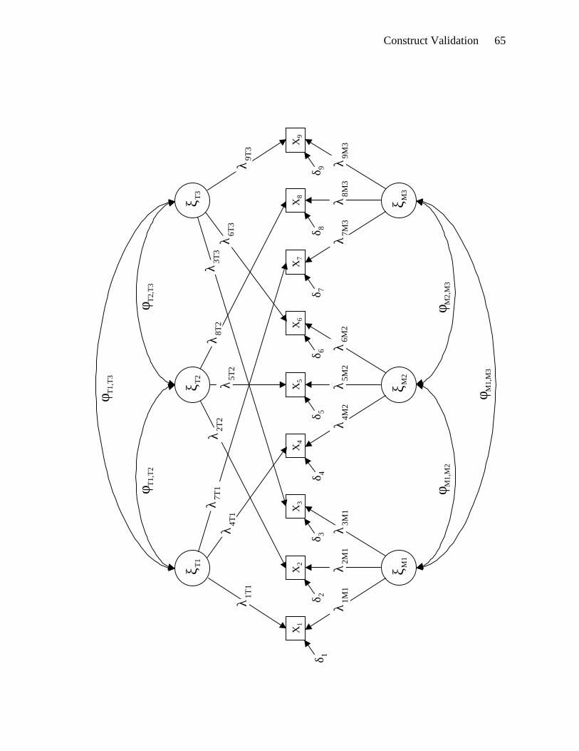
Construct Validation 65
X5
X6
X7
X8
X9
X1
X2
X3
X4
δ1
δ2
δ3
δ4
δ5
δ6
δ7
δ8
δ9
ξM
2 ξ
M1
ξM
3
λ1M
1 λ
2M1
λ3M
1 λ
4M2
λ5M
2 λ
6M2
λ7M
3 λ
8M3
λ9M
3
φ M1,
M2
φ M2,
M3
φ M1,
M3
ξT1
ξT2
ξT3
λ1T
1
λ6T
3 λ
4T1
λ7T
1 λ
2T2
λ5T
2
λ8T
2 λ
3T3
λ9T
3
φ T1,T
2φ T2
,T3
φ T1,T
3

Construct Validation 66
X1
X2 η
γ1
X3
γ3
γ2 ζφ13
φ12
φ23

Construct Validation 67
Y5
Y6
Y7
Y8
Y9
Y1
Y2
Y3
Y4
η2
η1
η3
λ11
λ21
λ31
λ42
λ52
λ62
λ73
λ83
λ93
ε1
ε2
ε3
ε4
ε5
ε6
ε7
ε8
ε9
ξ
γ 3 γ 2
γ 1
ζ 1
ζ 2
ζ 3

Construct Validation 68
X5
X6
X7
X8
X9
X1
X2
X3
X4
ξT1
ξT2
ξT3
λ1T
1
λ6T
3 λ
4T1
λ7T
1 λ
2T2
λ5T
2
λ8T
2 λ
3T3
λ9T
3
φ T1,T
2φ T2
,T3
φ T1,T
3
δ1
δ2
δ3
δ4
δ5
δ6
δ7
δ8
δ9
θδ 21
θδ 32
θδ 31
θδ 54
θδ 65
θδ 64
θδ 87
θδ 98
θδ 97